some of these slides have been borrowed from dr. paul...

Some of these slides have been borrowed from Dr.Paul Lewis, Dr. Joe Felsenstein. Thanks!

Paul has many great tools for teaching phylogenetics at his

web site:

http://hydrodictyon.eeb.uconn.edu/people/plewis

http://hydrodictyon.eeb.uconn.edu/people/plewis

Copyright © 2007 Paul O. Lewis 2

RuBisCO enzyme

8 small subunits (white)8 large subunits (colored)Responsible for fixing CO2


Green Plant rbcLM--S--P--Q--T--E--T--K--A--S--V--G--F--K--A--G--V--K--D--Y--K--L--T--Y--Y--T--P--E--Y--E--T--K--D--T--D--I--L--A--A--F--R--V--T--P--Chara (green alga; land plant lineage) AAAGATTACAGATTAACTTACTATACTCCTGAGTATAAAACTAAAGATACTGACATTTTAGCTGCATTTCGTGTAACTCCAChlorella (green alga) .....C...C.T....................T..CC..C.A.....C.....T...C.T..A..G..C...A.G.....TVolvox (green alga) ........TC.T.....A.....C..A.....C...GT.GTA.....C........C.....A.........A.G......Conocephalum (liverwort) ........TC..........T........G..T...G.............G..T........A......A.AA.G.....TBazzania (moss) ........T........C..T.....G.....A...G.G..C.....G..A..T.....G..A.........A.G.....CAnthoceros (hornwort) ........T........CC.T.....C.....T..CG.G..C..G........T.....G..A..G.C.T.AA.G.....TOsmunda (fern) ........TC....G...C..........C..T...G.G..C..G........T.....G..A.....C..AA.G.....CLycopodium (club "moss") .GG...............C.T..C........T.....G..C.....A..C..T...C.G..A........AA.G.....TGinkgo (gymnosperm; Ginkgo biloba) ..............G.....T...........A...C....C...........T..C..G..A.....C..A........TPicea (gymnosperm; spruce) ....................T...........A...C.G..C........G..T.....G..A.....C..A........TIris (flowering plant) ..............G.....T...........T..CG....C...........T..C..G..A.....C..A........TAsplenium (fern; spleenwort) ........TC..C.G.....T..C..C..C..A..C..G..C........C..T..C..G..A..T..C..GA.G..C...Nicotiana (flowering plant; tobacco) .....G....A...G.....T..............CC....C..G........T..A..G..A.....C..A........T

Q--L--G--V--P--P--E--E--A--G--A--A--V--A--A--E--S--S--T--G--T--W--T--T--V--W--T--D--G--L--T--S--L--D--R--Y--K--G--R--C--Y--H--I--E--CAACCTGGCGTTCCACCTGAAGAAGCAGGGGCTGCAGTAGCTGCAGAATCTTCTACTGGTACATGGACTACTGTTTGGACTGACGGATTAACTAGTTTGGACCGATACAAAGGAAGATGCTACGATATTGAA.....A..T........A........G..T..G........A........A..A........T.....G.....A........T..T...........A.....T........TC.T..T..T..C..C..G.....A..T...............TGT..T.....T..T.....T.....A..A..A.....T.....A.....A........T..T.....A...C.T.....T........TC.T..T..T..C..C..G..G.....G..A...G.A...........A..A.....T.....T..........................A...........T..TC.T....ACC.T..T..T..T.....TC.......T.G......C.....G..A..A.................A..G...........T........A..C.....G.....C..G........C..T..GC.T..A...C.C..T..T........TC.......T..C..C...T....A..G..G.................A..C...........T........A..........................C..T...C.T..C..CC.T.....T........TC..........C...........C..A..A..GG....G.....T..A..............G...........A.....G.....C.....A.....G..T...C.T..C...C.T..T..T..T..G..TC.....................T...A..A.....C..G.....G..A..C...........T........C..........................C..T...C.T..C...C.C..T..C........TC.G.....T..A..............A..G........G.....G..A..............C........C..............C...........C..T...C.T..C...C.T..T..T.....G...........T..C..C..G.....A..G..G..G..C..G.....G..A..A...........T........C..C...........C...........C..T...C.T......C.T..T..T.....G..GC.......T..C..C..G.....C..A.....TG..........G.....C..G........C.......................A..A..G........T...C.T..C...C.T..T..T.........C........C.C..C..G.....C..A..A...G..........C..A.................G..C.....A...........C.....G.....A.....G..G..C..CC.T.....T.....G..CC.............C..G........A.......................C..G........C.......................A.....A.....C..T...C.T..C..CC.T..T..T........GC........CGC..C..G

First 88 amino acids, translation is for Zea mays

All four bases are observed at some sites... ...while at other sites, only one base is observed

Question: Why is rate heterogeneity ubiquituous?

Answer: Differences in mutational rates and (mainly) selective constraint

• Many sites are under purifying (stabilizing) selection:– Any mutation results in a different amino acid, AND– A amino acid replacement at the site results in dramatically worse

functioning of the protein.– These sites will show low rates of evolution on a tree.

• Other sites are less constrained.– A mutation results in the same amino acid, OR– Many amino acids will work equally well at that position in the protein.– These sites will show high rates of evolution on a tree.

Rate heterogeneity in protein-coding genes: terms

• Synonymous mutations result in the same amino acid.

• Non-synonymous mutations result in the different amino

acid.

• Conservative changes are non-synonymous changes that

result in a chemically similar amino acid.

• Neutral mutations result in a new genotype that has

the same fitness as the genotypes currently fixed in the

population.

Rate heterogeneity in protein-coding genes: generalities

• Synonymous changes are often neutral (or close to neutral),

• Third base positions and untranslated regions (introns and

other non-coding regions) tend to have high rates because

changes to these sites lead to synonymous changes.

• Transitions tend to lead to more synonymous or conservative

changes.

• Amino acid residues that are embedded, involved in salt

bonding, or part of the active site tend to be more

constrained.

• Loops of amino acid residues on the outside of proteins often

tolerate a wide range of substitutions (or even indels).

2nd BaseU C A G

U

UUUF

UCU

S

UAUY

UGUC

UUC UCC UAC UGCUUA

LUCA UAA

*UGA *

UUG UCG UAG UGG W

C

CUU

L

CCU

P

CAUH

CGU

RCUC CCC CAC CGCCUA CCA CAA

QCGA

CUG CCG CAG CGG

A

AUUI

ACU

T

AAUN

AGUS

AUC ACC AAC AGCAUA ACA AAA

KAGA

RAUG M ACG AAG AGG

G

GUUV

GCU

A

GAUD

GGU

GGUC GCC GAC GGCGUA

LGCA GAA

EGGA

GUG GCG GAG GGG


Rate heterogeneity in RNA coding genes

• Stem regions– formed when RNA strand forms double-helix with

itself– strongly conserved in general– evidence for compensatory substitutions

• Loop regions– some strongly conserved– some entire loops are found in only particular lineages


Accommodating rate heterogeneityin substitution models

• Site-specific rates approach– e.g. let 1st, 2nd and 3rd position sites each have their own relative

substitution rate• Proportion of invariable sites approach

– assume that some proportion pinvar of sites have rate 0, while a proportion 1-pinvar have a rate > 0

• Discrete gamma distributed relative rates approach– assume that each site is evolving at one of ncat relative rates, where

the relative rates are determined using a gamma distribution having mean 1 and shape α

• Codon models (protein-coding genes only)– uses genetic code to determine appropriate relative rates

• Secondary structure models (RNA-coding genes only)– uses separate model for loops vs. stems, stem model takes account

of compensatory substitutions


Site-specific rates• You decide there are 3 classes of sites:

– 1st positions evolve at relative rate r1– 2nd positions evolve at relative rate r2– 3rd positions evolve at relative rate r3

• r1, r2 and r3 are relative rates, not actual rates:– their average is 1.0: if each category has the same number of

sites, (r1 + r2 + r3)/3 = 1.0– the actual rates are r1 α (for 1st positions), r2 α (for 2nd

positions) and r3 α (for 3rd positions)– note that the average substitution rate over all sites is α

(r1 α + r2 α + r3 α)/3 = α (1.0) = α• Assuming k rate classes adds k-1 parameters to the

model

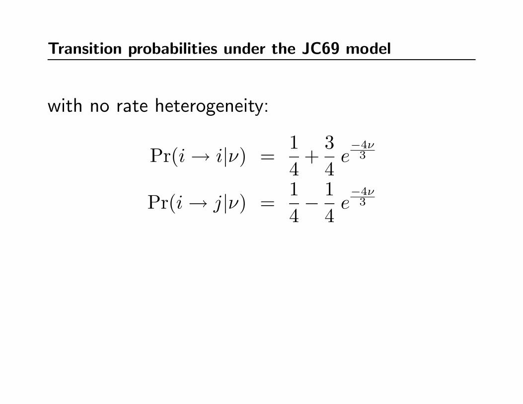
Transition probabilities under the JC69 model

with no rate heterogeneity:

Pr(i→ i|ν) =14

+34e−4ν3

Pr(i→ j|ν) =14− 1

4e−4ν3

Transition probabilities under the JC69 model

First base positions under a site-specific rates model:

Pr(i→ i|ν) =14

+34e−4r1ν

3

Pr(i→ j|ν) =14− 1

4e−4r1ν

3


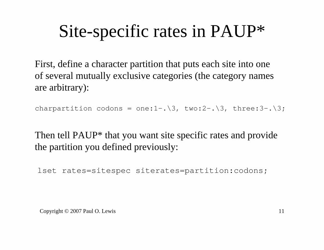
Site-specific rates in PAUP*

charpartition codons = one:1-.\3, two:2-.\3, three:3-.\3;

First, define a character partition that puts each site into oneof several mutually exclusive categories (the category namesare arbitrary):

lset rates=sitespec siterates=partition:codons;

Then tell PAUP* that you want site specific rates and providethe partition you defined previously:


Pinvar approach

• Unlike the site-specific rates approach, this approach does not require you to assign sites to rate categories

• Assumes there are only two classes of sites:– invariable sites (evolve at relative rate 0)– variable sites (evolves at relative rate r)

• Remarks:– mean of relative rates = (pinvar)(0) + (1-pinvar)(r) = 1– this means that r = 1/(1-pinvar)– if all sites are variable, pinvar = 0 and r = 1

• Constant site – a site in which all of the taxa

display the same character state.

• Invariable site – a site in which only one character

state is allowed. A site that cannot change state.

All invariable sites are constant, but not all constant

sites have to be invariable.

Pr(i→ i| invariable) =14

+34e−40ν

3

=14

+34e0

= 1

Pr(i→ j| invariable) =14− 1

4e−40ν

3

= 0

Why ν1−pinv

?

We want the mean rate of change to be 1.0 over all sites (so

we can interpret the branch lengths in terms of the expected

# of changes per site).

If r is the rate of change for the variable sites then:

1 = 0pinv + r(1− pinv

)= r

(1− pinv

)r =

11− pinv

Variable (but unknown) rates

• We expect more “shades of grey” rather than the on-or-off

view of the pInvar model.

• a priori we do not know which sites are fast and which are

slow

• We may be able to characterize the distribution of rates

across sites – high variance or low variance.


Gamma distributions

0

0.2

0.4

0.6

0.8

1

1.2

1.4

0 1 2 3 4 5

α = 10

α = 1

α = 0.1 smaller α meansmore heterogeneity

The mean equals1.0 for all three ofthese distributions

larger α meansless heterogeneity

The mean equals1.0 for all three ofthese distributions

relative rate

rela

tive

freq

uenc

y of

site

s

Gamma distribution

f(r) =rα−1βαe−βr

Γ(α)mean = α/β

mean (in phylogenetics) = 1

(in phylogenetics) β = α

variance = α/β2

variance (in phylogenetics) = 1/α

Using Gamma-distributed rates across sites

• We usually use a discretized version of the gamma with 4-8

categories (the computation time increases linearly with the

number of categories).

Pr(xi|JC +G) =ncat∑j

Pr(xi|JC, rjν) Pr(rj)

where:ncat∑j

rj Pr(rj) = 1

Discrete gamma (continued)

We “break up” the continuous gamma into intervals each

of which has an equal probability, and use the mean rate

within each interval as the representative rate for that rate

category:

Pr(rj) =1

ncatSo:

Pr(xi|JC +G) =1

ncat

ncat∑j

Pr(xi|JC, rjν)


Relative rates in 4-category case

0

0.2

0.4

0.6

0.8

1

0 0.5 1 1.5 2 2.5

Boundary between 1st and 2nd categories

Boundary between 2nd and 3rd categories

Boundary between 3rd and 4th categories

Boundaries are placed so that each category represents 1/4 of the distribution (i.e. 1/4 of the area under the curve)

r1 = 0.137 r2 = 0.477 r3 = 1.000 r4 = 2.386

Relative ratesrepresent themean of theircategory


Discrete gamma rate heterogeneity in PAUP*

To use gamma distributed rates with 4 categories:

To estimate the shape parameter:

lset rates=gamma ncat=4;

lset shape=estimate;

lset rates=gamma shape=0.2 pinvar=0.4;

To combine pinvar with gamma:

Note: estimate, previous, or a specific value can be specified for both shape and pinvar


Rate homogeneity in PAUP*

lset rates=equal pinvar=0;

Just tell PAUP* that you want all rates to be equal and that you want all sites to be allowed to vary:

Note: these are the default settings, but it is useful to know how to go back to rate homogeneity after you have experimented with rate heterogeneity!

Copyright © 2007 by Paul O. Lewis 2

Likelihood ratio test• Always compares an unconstrained to a

constrained model• Constrained model must be nested within the

unconstrained model• Parameter(s) take on their maximum likelihood

estimates (MLEs) in the unconstrained model• Parameters(s) set to some other value of interest in

the constrained model• Unconstrained model must be able to attain a

higher maximum likelihood than the constrained model


is the MLE

is some other value

Likelihood Ratio Test

Coin-flipping example:Data: 6 heads out of 10 flipsConstrained model: fair coin (θ = 0.5)Unconstrained model: biased coin (θ = )

Example of likelihood calculation for case of θ = 0.6


Likelihood Ratio TestCoin-flipping example:

Data: 6 heads out of 10 flipsConstrained model: fair coin (θ = 0.5)Unconstrained model: biased coin (θ = )

LRT approximates a chi-square random variable with d.f. equal to the difference in the number of free parameters between the two models

Not significant: P = 0.527

This means that thesimpler, constrained

model cannot be rejected


Examples of unconstrained vs. constrained model comparisons

1. GTR+G (shape=MLE) vs. GTR (shape=∞)2. K80 (κ=MLE) vs. JC (κ=1.0)3. HKY+I+G (pinv=MLE) vs. HKY+G (pinv=0)4. HKY+I+G (pinv=MLE, shape=MLE)

vs. HKY (pinv=0, shape= ∞)Note: cases in which the constrained model involves setting aparameter to the edge of its valid range (e.g. cases 1, 2 and 4 above) require special consideration (see Ota et al. 2000)

Ota, R., P. J. Waddell, M. Hasegawa, H. Shimodaira, and H. Kishino. 2000. Appropriate likelihood ratio tests and marginal distributions for evolutionary tree models with constraints on parameters. Molecular Biology and Evolution 17:798-803.


Testing the molecular clock

1 2 3 4 5 6 7

t1 t2 t3 t4 t5

Unconstrained model: need to estimate 2n-3 = 11 branch lengthsConstrained model: need to estimate n-1 = 6 divergence times

Likelihood ratio test thus has (2n-3) - (n-1) = n-2 d.f.

t6

n = 7 taxa


Akaike Information Criterion

• AIC = -2 max(lnL) + 2K• K is number of free model parameters• Measures relative distance to true model• Model with smallest AIC wins• Advantage over LRT: non-nested models

Example: 6 heads/10 flips revisitedUnconstrained model: θ = 0.6, AIC = -2(-1.383) + 2(1) = 4.766Constrained model: θ = 0.5, AIC = -2(-1.584) + 2(0) = 3.168 (best)


Bayesian Information Criterion• BIC = -2 max(lnL) + K log(n)• K is number of free model parameters• n is the sample size• Model with smallest BIC wins• Advantage over LRT: non-nested models• Considered superior to both AIC and LRT

Example: 6 heads/10 flips one more time. Note: log(10) ≈ 2.3Unconstrained model: θ = 0.6, BIC = -2(-1.383) + (2.3)(1) = 5.066Constrained model: θ = 0.5, BIC = -2(-1.584) + 0 = 3.168 (best)


Likelihood ratio test favorsmore complex models

• Assume the simpler, constrained model is the true model

• If the LRT was statistically consistent, it would choose the true model with certainty as n→∞

• But the simpler model will be rejected 5% of the time, regardless of sample size

• Thus, LRT biased toward choosing the more complex, unconstrained model

References

some of these slides have been borrowed from dr. paul...

Documents