some physical models of the reaction ... physical models of the reaction-diffusion equation and...

SOME PHYSICAL MODELS OF THEREACTION-DIFFUSION EQUATION AND COUPLED

MAP LATTICES

YAKOV PESIN AND ALEX YURCHENKO

Abstract. We review a number of models which appear in physics,biology, chemistry, etc. and which are described by the reaction-diffusion equation. By discretazing this equation we obtain thecorresponding coupled map lattice (CML) system. We classifythese CMLs by the type of the dynamics of the local map. Weobserve several different types of behavior, namely, Morse-Smaletype systems, systems with attractors, and systems with Smalehorseshoes.

1. Introduction.

In this paper we review a number of important models in physics,biology, and chemistry which are described by the non-linear reaction-diffusion equation

ut = h(u) +Aκ4u,where x ∈ Rp, u = u(x, t) is a function with values in Rd, A a matrix,and κ a parameter. This equation represents extended systems of un-bounded equilibrium media with energy pumping and the function u isa characteristic of the medium (for example, its density, or distributionof temperature). In Section 2 we discribe the models while in Section3 we classify them according to their type.

We are interested in the dynamics of the corresponding coupled maplattice (CML) that is a discrete versions of this equation, i.e.,

uj(n+ 1) = f(uj(n)) + εgj(ui(n)|i−j|≤s),where n ∈ Z is the discrete time coordinate and j = (jk), k = 1, ..., pthe discrete space coordinate. We assume that f : Rd → Rd and

Date: April 25, 2004.1991 Mathematics Subject Classification. Primary: 37N25, 37N10, 35K57.Key words and phrases. Coupled Map Lattices, amplitude equation, reaction-

diffusion equation, Morse-Smale system, Smale horseshoe, attractor, FitzHugh-Nagumo.

The work was partially supported by the National Science Foundation grant#DMS-0088971 and U.S.-Mexico Collaborative Research grant 0104675.

1

2 YAKOV PESIN AND ALEX YURCHENKO

gj : (Rd)(2s+1)p → Rd are smooth maps; f is called the local map and itacts in the local phase space (which is either Rd or its compactificationSd); g is the interaction of finite size s. We also assume that ε is asufficiently small parameter (see Section 4).

One can think of a CML as an infinite collection of copies of thelocal dynamical system (f,Rd) associated with each point in the latticeZd. When ε = 0 the local dynamics at different points of the latticedo not depend on each other. However, for small ε the dynamics ata given point of the lattice ”feels” the local dynamics at neighboringpoints (within the lattice cube of size s). In the cases, where the localdynamics displys strong hyperbolic behavior, the dynamics of CML iscompletely determined by the local dynamics (provided ε is sufficientlysmall). See [1, 2]. The goal of this paper is to analize the local dynamicsin some ”physicall interesting” cases.

When a CML is obtained from a partial differential equation (PDE)there are two ways to ensure that ε is small: 1) to require that thecorresponding parameter of the PDE (usually the diffusion coefficient)is small and 2) to select small discretization steps appropriately.

In what follows, we will fix the discretization step and will vary ”thephysical parameters” of the system. It turns out that CML’s obtainedin this way can often be viewed as initial phenomenological models ofthe underlying processes and in many cases may be better adopted tothem.

In the Sections 5 and 6 we classify CML under consideration by thetype of the dynamics of their local maps. It turns out that when thelocal map is one-dimensional the dynamics is of Morse-Smale type insome range of parameters. When the local map is the two-dimensionalthe dynamics is much richer: by varying parameters of the system onecan observe a Morse-Smale type behavior, existence of Smale horse-shoes, or “strange” attractors. We illustrate this by study of the dy-namics of the local map of the FitzHugh-Nagumo equation (see Section6).

Acknowledgement. The authors would like to thank D. Anosovfor some valuable comments and Ke Zhang, a graduate student atPenn State University, for careful reading of the manuscript and manycorrections. Ya. P. also would like to thank RIMS at Kyoto University,where the final version of the paper was prepared, for support andhospitality.

PHYSICAL MODELS OF THE REACTION-DIFFUSION EQUATION 3

2. Models From Science.

Here we present several examples from different branches of sciencethat are described by evolution PDE’s.

2.1. Fisher model in population genetics [26]. The model de-scribes a population of diploid individuals (i.e., the ones that carrytwo genes) distributed in a flat two dimensional habitat. Assumingthat a gene occurs in two forms a and A, called alleles, one can dividethe population into three genotypes aa, aA, and AA. Let ui = ui(t, x),i ∈ 1, 2, 3, be the population densities of aa, aA, and AA respec-tively. Assume that members of the population mate at random, witha birth rate r, and diffuse through the habitat with a diffusion constantD. Assume further that death rates depend only on the genotypes anddenote them by τi, i = 1, 2, 3. Thus, ui(x, t) changes due to diffusion,mating, and death.

It is shown in [3] that if |τ1 − τ2|+ |τ3 − τ2| 1 and r 1 then thefunction

u =u3 + 1

2u2

u1 + u2 + u3

satisfies the following PDE

(2.1.1) ut = −σu(u− θ)(u− 1) +D4u,where σ = σ(τ1, τ2, τ3) > 0 and θ = θ(τ1, τ2, τ3), 0 < θ < 1 are parame-ters.

2.2. Kolmogorov-Petrovskii-Piskunov (KPP) planar model ofadvance of advantageous genes [16]. Consider a two dimensionalarea populated by individuals of a given species. Assume that thepopulation has a dominant allele A, that is, the chance of survival ofindividuals with this allele is larger than individuals that do not possesthis gene.

In the case when the dominant allele is distributed over the area witha constant concentration p the change of p per one generation can beobtained by the formula (see [9])

δp = αp(1− p)2 +O(α2),

where α+1 is the ratio of the probability that an individual with domi-nant allele A survives to the corresponding probability for an individualwithout the allele A.

We now consider the case when the concentration p changes in timeand space due to the selection in favor of the dominant allele A andto random motions of individuals. Assume finally that the root-mean-square path ρ of an individual during one generation is sufficiently


small. One can show that the change in the concentration per genera-tion can be found by the formula(2.2.2)

δp(x, y) =

∫

R

∫

Rp(ζ, ξ)

f(r)

2πrdζdξ − p(x, y) + αp(x, y)(1− p(x, y))2,

where f(r)dr is the probability that an individual passes a distance

lying between r and r + dr with r =√

(x− ζ)2 + (y − ξ)2. Assumingthat p is differentiable with respect to the coordinates x, y, and time tand that α 1 we can expand (2.2.2) into a Taylor series to obtain

(2.2.3) pt = αp(1− p)2 +ρ2

44p.

2.3. Fisher linear model of advance of advantageous genes [10].Consider a population of a given species distributed uniformly along alinear habitat, such as a shore line. Assume that the size of the habitatis large compare with the distances separating the sites of offspringsfrom those of their parents. Assume further that at some point of thehabitat an advantageous mutation (that is a mutation that is somehowadvantageous to the survival of a member of the population) occurs.This mutation diffuses, first, into the neighborhood of the occurrenceof mutation and then into the surrounding population. This process isdue to selection in favor of the advantageous mutation and to randommotions of individuals.

Let p = p(x, t) be the concentration of the members of the populationwith the mutant gene and q = q(x, t) the concentration of the membersof the population whose offsprings have the mutant gene (x is a positionin the habitat). One can assume that q = 1 − p. Denote by α theintensity of selection in favor of the mutant gene, which we assume tobe independent of p. For sufficiently small α the concentration p variescontinuously with time from generation to generation. Suppose thatthe rate per generation at which members of the population with themutant gene diffuse into the whole population is given by −κ ∂p

∂x, where

κ > 0 is a diffusion constant (assumed to be independent of x andp). This corresponds to the ordinary law of diffusion that is diffusionis proportional to the gradient of the concentration. Under all theseassumptions one can show that the concentration of the mutant genesatisfies:

(2.3.4)∂p

∂t= αp(1− p) + κ

∂2p

∂x2.


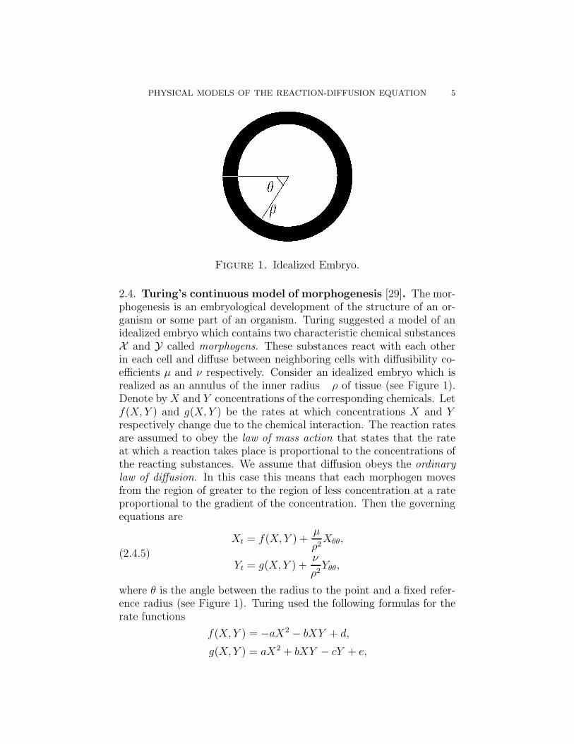
Figure 1. Idealized Embryo.

2.4. Turing’s continuous model of morphogenesis [29]. The mor-phogenesis is an embryological development of the structure of an or-ganism or some part of an organism. Turing suggested a model of anidealized embryo which contains two characteristic chemical substancesX and Y called morphogens. These substances react with each otherin each cell and diffuse between neighboring cells with diffusibility co-efficients µ and ν respectively. Consider an idealized embryo which isrealized as an annulus of the inner radius ρ of tissue (see Figure 1).Denote by X and Y concentrations of the corresponding chemicals. Letf(X, Y ) and g(X, Y ) be the rates at which concentrations X and Yrespectively change due to the chemical interaction. The reaction ratesare assumed to obey the law of mass action that states that the rateat which a reaction takes place is proportional to the concentrations ofthe reacting substances. We assume that diffusion obeys the ordinarylaw of diffusion. In this case this means that each morphogen movesfrom the region of greater to the region of less concentration at a rateproportional to the gradient of the concentration. Then the governingequations are

Xt = f(X, Y ) +µ

ρ2Xθθ,

Yt = g(X, Y ) +ν

ρ2Yθθ,

(2.4.5)

where θ is the angle between the radius to the point and a fixed refer-ence radius (see Figure 1). Turing used the following formulas for therate functions

f(X, Y ) = −aX2 − bXY + d,

g(X, Y ) = aX2 + bXY − cY + e,


where a, b, c, d, e ∈ R+ are parameters of the reaction.

2.5. Maginu model of morphogenesis [17]. This model is a sim-plification of the above Turing model. A single cell is viewed as anelectrical circuit similar to the one used by Nagumo (see Section 2.8below and Figure 3). Arranging these cells on a ring by coupling neigh-boring ones, Maginu produced a system of reaction-diffusion PDE’s

Xt = −aX(X − 1)(X + 1)− Y + κ1Xθθ,

Yt = ε(X − γY ) + κ2Yθθ,(2.5.6)

where X and Y are concentrations of two types of morphogens, a, κ1,κ2, ε, and γ are positive parameters. Note that the nonlinear term in(2.5.6) is simpler than the nonlinear term in (2.4.5).

2.6. The FitzHugh’s model of the propagation of voltage im-pulse through a nerve axon. In [14], Hodgkin and Huxley proposeda model to describe the ionic and electrical events occurring duringthe transmission of an impulse through the surface membrane and thepropagation of voltage impulse through a nerve axon. One can thinkof the axon as a long cylindrical cable with a conducting core and apartially insulating shell submerged into a large volume of conductingfluid - an ionic solution of either sodium or chloride.

The total density I of the current through the membrane is

(2.6.7) I = CMdV

dt+ Ii,

where V is the displacement of the membrane potential from its restingvalue; CM the membrane capacity per unit area (assumed to be con-stant); and Ii = INa(V )+IK(V )+Il(V ) the ionic current density whichconsists of three components carried by: sodium ions (INa), potassiumions (IK), and other ions (Il). The expression for ionic currents densi-ties INa, IK , and Il were obtained experimentally.

The current density through the membrane can be computed by theformula

(2.6.8) I =ρ

2R

∂2V

∂x2,

where x is the distance along the fibre, R the specific resistance of theaxoplasm, and ρ the radius of the fibre. Combining (2.6.7) and (2.6.8)we obtain that

ρ

2R

∂2V

∂x2= CM

dV

dt+ Ii(V ).


The Hodgkin-Huxley model consists of four differential equations andis yet to difficult for rigorous mathematical analysis. For the detaileddiscussion of Hodgkin-Huxley model see [6].

In [11], R. FitzHugh suggested a model for the propagation of voltageimpulse through a nerve axon which is substantially simpler than theHodgkin-Huxley model and therefore, is often used in applications.

R. FitzHugh treated the nerve cell as a non-linear electric oscillator

v + (v2 − 1)v + cv = 0,

where v is a dimensionless variable corresponding to the membranepotential V and c > 0 a constant. Setting

w = −v + v − v3

3

reduces the above second order differential equation to the well-knownBonhoeffer-van der Pol (BVP) system of differential equations of thefirst order

v = v − v3

3− w,

w = cv.

The variable w is called the recovery variable. R. FitzHugh furthermodified this system as follows

v = v − v3

3− w + i,

w = c(v + a− bw),(2.6.9)

where a and b are positive constants and i a dimensionless variable cor-responding to the total membrane current density. Combining (2.6.9)and (2.6.8) we obtain the system of two differential equations:

vt = v − v3

3− w + κvxx

wt = c(v + a− bw).(2.6.10)

where κ is proportional to ρ2R

. If no recovery is present (i.e., w = 0)we obtain the one-dimensional FitzHugh model (see [12]):

(2.6.11) vt = v − v3

3+ κvxx.


2.7. Brusselator model for the Belousov-Zhabotinsky reaction(BZR) [8]. The BZR is a chemical reaction in which the concentra-tions of the reactants exhibit oscillating behavior. The Brusselatormodel of BZR describes the case of a single mode of oscillation towhich the system returns if perturbed. The chemical reactions followthe scheme:

A → XB + X → Y +D

2X + Y → 3XX → E

where A, B, D, E , X , and Y are chemical compounds. Let x and ybe the concentration of compounds X and Y and A and B the con-centrations of compounds A and B. Assuming that the concentrationA and B are held constant during the chemical reaction and that thesystem has only one spatial dimension one obtains the following systemof differential equations

∂x

∂t= A− (B + 1)x+ x2y +D1

∂2x

∂ξ2

∂y

∂t= Bx− x2y +D2

∂2y

∂ξ2

(2.7.12)

where D1 and D2 are diffusion constants and ξ is the spatial coordinate.

2.8. Bistable transmission lines [22]. One can simulate an activetransition line with two stable equilibrium states in the following way.Consider a circuit which consists of a power source E0, resistance R,capacitor C, and tunnel diode with characteristic curve f(v) to be acubic polynomial (see Figure 2). One can set E0 and R such that thecircuit acts as a bistable circuit. The equations of the circuit are givenby

j = Cdv

dτ+ g(v),

g(v) = f(v) +v − E0

R,

where j is the current and v the potential; the function g(v) is a cubicpolynomial,

g(v) = a(v − v1)(v − v2)(v − v3),

where a > 0 and v1 < v2 < v3.


Figure 2. The circuit of the simple bistable line.

Figure 3. The distributed bistable line.

Regarding this circuit as a distributed line (see Figure 3) we obtain

j =1

r

∂2v

∂s2,

where s is the distance along the line and r the interstage coupling re-sistance per unit length of the line. By appropriate change of variableswe obtain

(2.8.13)∂u

∂t= −(u+ 1)(u− θ)(u− 1) + κ

∂2u

∂s2,


Figure 4. The plane Poiseuille flow.

where θ, −1 < θ < 1 and κ are parameters of the circuit and u therescaled voltage.

2.9. Wave system in plane Poiseuille flow [28]. The Poiseuilleflow is a planar flow of an incompressible viscous fluid under pressurein a channel made up by two parallel plates with distance 2h betweenthem (see Figure 4). Under the uniform pressure gradient the flowproduces a velocity field which is independent of the x coordinate andhas its maximum value u0 at the center of the channel. The governingequation of the flow is

(2.9.14) ζt + ψzζx − ψxζz =1

R4ζ,

where R = 1γu0h is the Reynolds number, γ the kinetic viscosity, ψ =

ψ(x, z, t, R) the stream function, ζ = −4ψ, x the direction parallel tothe plates, and z the direction perpendicular to the plates. The timeis measured in h

u0units, the length in h units, and the velocity in u0

units. For the incompressible flow (i.e. ∇~u = 0) the stream function ψis defined by

~u = ∇⊥ψ,where ~u is the velocity field and ∇⊥ := (∂z,−∂x).

In the case of the undisturbed laminar flow (called the basic flow)the motion is parallel to the plates and is given by the mean velocitywith respect to x

u` :=∂ψ`∂z

= 1− z2,

where ψ` is the stream function of the undisturbed laminar flow.Consider a small disturbance which is confined to a small neigh-

borhood of the origin at t = 0. Linearization of the (2.9.14) around


the basic flow gives the following equation for the perturbed streamfunction ψ

(2.9.15)

(∂

∂t+ (1− z2)

∂

∂x

)4ψ + 2

∂ψ

∂x=

1

R42ψ.

One can obtain a formal solution of (2.9.15) using the Fourier-Laplacetransform

ψ(z, α, s, R) =

∫ ∞

0

e−stdt

∫

Re−iαxψ(x, z, t, R)dx,

ψ(x, z, t, R) = ψ(z) =1

4π2i

∫

Reαixdα

∫ γ+i∞

γ−i∞estψ(z, α, s, R)ds.

where the line Re(s) = γ lies to the right of all singularities of ψ. Solv-ing the above equation for ψ leads to the Orr-Sommerfeld eigenvalueproblem

− iα((

1− z2 − is

α

)(dψ(2)

dz2− α2ψ

)+ 2ψ

)

+1

R

(dψ(4)

dz4− 2α

dψ(2)

dz2+ α4ψ

)= 0.

Fix R and let s(α) be the eigenvalues of the non-trivial solution.One can show that there is a critical value Rc such that for all R < Rc,the real part of each eigenvalue s(α) is less than zero and for R > Rc

there are eigenvalues with positive real part. Hence, for R > Rc thebasic flow is unstable under the small disturbances and for R < Rc itis stable.

The experiments however, show that even for R < Rc the basic flowcan be unstable. Thus the linear analysis is not sufficient to studystability of the basic flow and some non-linear terms should be takeninto account.

For that we consider a small perturbation of the basic flow whoseReynolds number R is sufficiently close to the critical value Rc. Wethen expand solutions into powers of R − Rc and study the leadingFourier mode of the expansion. One can show that its amplitude Asatisfies the following equation

(2.9.16) At = kA |A|2 + εA+ aAxx,

where |ε| 1 and k, a are complex parameters; moreover, ε > 0 ifR > Rc and ε < 0 otherwise.


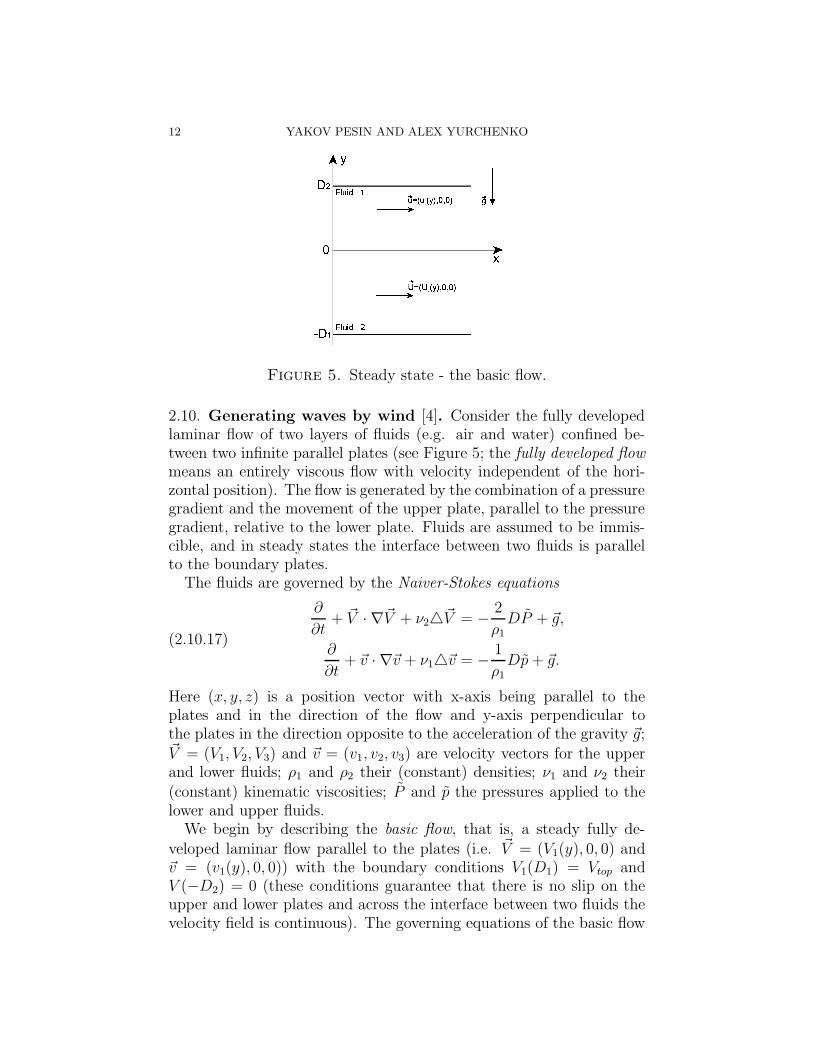
Figure 5. Steady state - the basic flow.

2.10. Generating waves by wind [4]. Consider the fully developedlaminar flow of two layers of fluids (e.g. air and water) confined be-tween two infinite parallel plates (see Figure 5; the fully developed flowmeans an entirely viscous flow with velocity independent of the hori-zontal position). The flow is generated by the combination of a pressuregradient and the movement of the upper plate, parallel to the pressuregradient, relative to the lower plate. Fluids are assumed to be immis-cible, and in steady states the interface between two fluids is parallelto the boundary plates.

The fluids are governed by the Naiver-Stokes equations

∂

∂t+ ~V · ∇~V + ν24~V = − 2

ρ1DP + ~g,

∂

∂t+ ~v · ∇~v + ν14~v = − 1

ρ1

Dp+ ~g.

(2.10.17)

Here (x, y, z) is a position vector with x-axis being parallel to theplates and in the direction of the flow and y-axis perpendicular tothe plates in the direction opposite to the acceleration of the gravity ~g;~V = (V1, V2, V3) and ~v = (v1, v2, v3) are velocity vectors for the upperand lower fluids; ρ1 and ρ2 their (constant) densities; ν1 and ν2 their(constant) kinematic viscosities; P and p the pressures applied to thelower and upper fluids.

We begin by describing the basic flow, that is, a steady fully de-veloped laminar flow parallel to the plates (i.e. ~V = (V1(y), 0, 0) and~v = (v1(y), 0, 0)) with the boundary conditions V1(D1) = Vtop andV (−D2) = 0 (these conditions guarantee that there is no slip on theupper and lower plates and across the interface between two fluids thevelocity field is continuous). The governing equations of the basic flow


are

0 =G

ρ2+ ν2

d2V1

dy2,

0 =G

ρ1

+ ν1d2v1

dy2,

where∂P

∂x=∂p

∂x= −G

is the constant pressure gradient and p = p + ρ1gy and P = P + ρ2gyare modified pressures. Let Vb(y), vb(y), Pb, pb be the solution of thissystem (with boundary conditions discussed above). These solutionsdepend linearly on G and Vtop. We introduce the dimensionless veloci-ties

Vb =Vb

Vmean, vb =

vbVmean

,

where Vmean is the mean velocity

Vmean =1

D1 +D2

(∫ 0

−D1

vbdy +

∫ D2

0

Vbdy

).

We also introduce the Reynolds number R = VmeanD2

ν2.

The ”wind” can be viewed as a perturbation of the basic flow forwhich the velocity field can be represented in the form

~v = (vb, 0, 0) + δ cos(kx + lz − kct) (v1(y), v2(y), v3(y)) ,

~V = (Vb, 0, 0) + δ cos(kx+ lz − kct) (V1(y), V2(y), V3(y)) ,

and the pressures

p = pb + δp(y) cos(kx + lz − kct),P = Pb + δp(y) cos(kx + lz − kct).

Here δ 1, k, l ∈ C are disturbance wave numbers in x- and z-directions respectively, and c ∈ C the phase speed. This kind of per-turbation is considered frequently in the systems with translationalinvariance. It corresponds to the study of the stability of the Fouriermodes (which represents delocalized disturbances) ([7]).

The perturbed system is governed by the Navier-Stokes equation(2.10.17) with boundary conditions as above and the velocity field beingcontinuous across the interface y = η(x, z, t) where

η(x, z, t) = δ cos(kx + lz − kct).To study stability of the basic flow we substitute the values of pres-

sures and velocities into (2.10.17) and linearize this system along the


basic flow. One can show that in the (R, k)-plane there exists the sta-bility curve, i.e., a curve that divides the (R, k)-plane into two regionsin which the basic flow is stable and unstable respectively. This curvehas a critical point (Rc, kc) for which kc 6= 0.

Now, consider a small perturbation of the basic flow whose Reynoldsnumber R is sufficiently close to the critical value Rc. By expandingsolutions of (2.10.17) into powers of R−Rc one can show that

(2.10.18) At = bA + kA |A|2 + aAxx,

where A is the leading Fourier mode of the expansion (i.e. amplitudeof the surface wave is proportional to A), a a complex parameter withpositive real part, b a complex parameter which is related to the expo-nential growth of the wave for R > Rc, and k is a complex parameterwhich is related to the motion in the bulk of the fluid and nonlineareffects at the interface.

3. A Classification of Models.

A non-linear reaction-diffusion equation is a PDE of the form:

(3.0.19) ut(x, t) = h(u) +Aκ∆xu(x, t),

where u(x, t) is a function of space coordinate x ∈ Rn and time t ≥ 0with values in Rd; A is the coupling matrix, and κ a diffusion coefficient.One can obtain a number of well-known equations by the appropriatechoice of the nonlinear term h.

3.1. The Kolmogorov-Petrovsky-Piskunov (KPP) Equation. TheFisher linear model and the KPP planar model of advance of advan-tageous genes (Equations (2.3.4) and (2.2.3)) are examples of the gen-eralized KPP equation introduced in [16]. This is a one-dimensionalreaction-diffusion equation

(3.1.20) ut(x, t) = h(u) + κ4u(x, t), 0 ≤ u ≤ 1,

where the nonlinear term h(u) ∈ C1([0, 1]) satisfies the following con-ditions:

(3.1.21) h(0) = h(1) = 0, h′(0) = α > 0, h′(u) < α, u ∈ (0, 1],

For the Fisher model we have h(u) = αu(1 − u) and for the KPPmodel h(u) = αu(1− u)2.


3.2. The FitzHugh-Nagumo Equation. The FitzHugh modelof propagation of voltage impulse through a nerve axon (Equation(2.6.10)) and Maginu model of morphogenesis (Equation (2.5.6)) aredescribed by the FitzHugh-Nagumo generalized equation. It is a two di-mensional reaction-diffusion equation with u(x, t) = (u1(x, t), u2(x, t)),x ∈ R and

h(u1, u2) = (n(u1)− bu2, cu1 − du2),

A =

(σ1 00 σ2

),

where a, b, c, d, and σi are positive parameters, σi ∈ 0, 1, i = 0, 1,and

n(u1) = −au1(u1 − θ)(u1 − 1)

with θ ∈ (0, 1). The equations become

∂u1

∂t= −au1(u1 − θ)(u1 − 1)− bu2 + κ1

∂2u1

∂x2

∂u2

∂t= cu1 − du2 + κ2

∂2u2

∂x2.

(3.2.22)

where κi ≥ 0 and at least one of them is nonzero.

3.3. Nagumo Equation. The one-dimensional FitzHugh model ofpropagation of voltage impulse through a nerve axon (Equation (2.6.11)),the Fisher model in population genetics (Equation (2.1.1)), and bistabletransition lines (Equation (2.8.13)) are described by the Nagumo equa-tion. The latter is a special case of the more general semi-linear bistablereaction-diffusion equation

(3.3.23) ut(x, t) = h(u) + κuxx(x, t),

where the nonlinear term is given by

h(u) = −au(u− θ)(u− 1),

with a > 0 and θ ∈ (0, 0.5]. Note that the case θ ∈ (0.5, 1) can bereduced to the previous one by replacing u with −u+1. Also note thatEquation (3.3.23) is the first equation in the system (3.2.22) for b = 0.

3.4. The Real Ginzburg-Landau (Amplitude) Equation. Theamplitude of the disturbance in the Poiseuille flow (Equation 2.9.16)and amplitude of the waves generated by wind (Equation 2.10.18) areall described by the amplitude equation. A general complex Ginzburg-Landau equation is given by

ut(x, t) = βu|u|2 − γu+ α∆xu(x, t),


where α, β ∈ C, and γ ∈ R are parameters, u ∈ C. Here we onlyconsider a one dimensional real version of this equation given by

(3.4.24) ut(x, t) = u(γ − δu2) + κuxx(x, t),

where γ, δ, κ ∈ R. Note that if γ, δ, κ > 0 Equation (3.4.24) becomes(after rescaling) the Nagumo equation (3.3.23).

3.5. Some Other Non-linear Reaction-Diffusion Equations. TheBrusselator model for the Belousov-Zhabotinsky reaction (Equation2.7.12) gives us another two dimensional reaction-diffusion equation

∂u1

∂t= A− (B + 1)u1 + u2

1u2 + κ1∂2u1

∂x2,

∂u2

∂t= Bu1 − u2

1u2 + κ2∂2u2

∂x2.

(3.5.25)

where A, B, κi, i = 0, 1 are positive parameters.Finally, from the Turing model of morphogenesis (Equation 2.4.5)

we obtain yet another two dimensional system

∂u1

∂t= −(au2

1 + bu1u2) + c+ κ1∂2u1

∂x2,

∂u2

∂t= (au2

1 + bu1u2)− du2 + e+ κ2∂2u2

∂x2.

(3.5.26)

where a, b, c, d, e, and κi, i = 0, 1 are positive parameters.

4. Coupled Map Lattices (CML).

To construct CMLs which correspond to the PDEs described abovewe use the following discretization. For the derivative in time

∂u(x, t)

∂t→ u(x, t+ ∆t)− u(x, t)

∆t.

For the space derivative one can choose any discretization method in-volving an arbitrary number of points. For example,

∂u(x, t)

∂x→ u(x+ ∆x, t)− u(x, t)

∆x∂u2(x, t)

∂x2→ u(x+ ∆x, t)− 2u(x, t) + u(x−∆x, t)

(∆x)2,

where ∆t and ∆x are the discretization steps.Using the above discretization we obtain the CMLs corresponding

to the above mentioned PDEs. We describe below the local maps forthese CMLs and indicate leading parameters, i.e., the parameters thatwe will vary to obtain different types of dynamics.


• The KPP equation:

f(u) = u+ γh(u),

where h(u) satisfies (3.1.21), h′(0) = α is a leading parameterand γ = ∆t > 0 is a parameter.• The Nagumo equation:

f(u) = u− Au(u− θ)(u− 1),

where A = α∆t > 0 is a leading parameter and θ ∈ (0, 0.5) is aparameter.• The real amplitude equation:

f(u) = Au− bu3,

where A = (1 +γ∆t) > 0 is a leading parameter and b = δ∆t ∈R is a parameter.• The FitzHugh-Nagumo equation:

f(u1, u2) = (u1 − Au1(u1 − θ)(u1 − 1)− αu2, βu1 + γu2),

where A = a4t > 0 is a leading parameter, α = b4t > 0,β = c∆t > 0, γ = (1− d∆t) > 0, θ ∈ (0, 1) are parameters.• The Brusselator model:

f(u1, u2) = (a+ (1− γ − b)u1 + γu21u2, u2 + bu1 − γu2

1u2),

where a = A4t > 0, b = B∆t > 0 are two leading parameters,and γ = 4t > 0 is a parameter.• The Turing model:

f(u1, u2) = (u1 − Au21 − Bu1u2 + C,

Au21 +Bu1u2 + (1−D)u2 + E),

where A = a4t > 0, B = b∆t > 0, C = c∆t > 0, D = d∆t > 0,and E = e∆t > 0 are parameters.

The interaction g is a function of 2s+ 1 variables, where in our cases = 1.

5. Dynamics of Local Map: One Dimensional Maps.

We consider the case of one-dimensional local maps. We show thatin some range of parameters they exhibit Morse-Smale type behavior.

5.1. KPP Equation. We begin with the KPP equation and considerlocal maps of two types: (1) f(u) = u + γu(1 − u) and (2) f(u) =u+ γu(1− u)2.


Figure 6. Phase Portraits of 1-dimensional maps: a)KPP equation, f(u) = u + γu(1 − u), 0 < γ < 1; b)Nagumo equation, f(u) = u− Au(u− θ)(u− 1), A < 1;c) real amplitude equation, f(u) = Au− bu3.

Figure 7. The local map of the KPP equation, f(u) =u+ γu(1− u), γ < 1.

5.1.1. The local map f(u) = u + γu(1 − u). Assume that 0 < γ < 1and let u1 = 1

2+ 1

2γ> 1. The derivative f ′(u) = 1 + γ(1− 2u) > 0 for

u < u1 while f ′(u1) = 0 (see Figure 7). The local map has two fixedpoints: u = 0 is repelling (f ′(0) = 1 + γ > 1) and u = 1 is attracting(f ′(1) = 1− γ < 1). We change f outside of [0, u1] such that the newmap (still called f) has a repelling fixed point u = P and f ′(u) > 0


Figure 8. The modified local map of the KPP equation.

Figure 9. The local map of the KPP equation, f(u) =u+ γu(1− u), γ > 1 +

√5.

for all u ∈ R and f ′(u) > 1 for u > P (see Figure 8). The new mapis a diffeomorphism of R with three fixed points and no other periodicpoints. Let f be the compactification map of f (see Appendix).

Theorem 5.1.1. For all γ ∈ (0, 1) the compactification map f is aMorse-Smale diffeomorphism of S1 with four fixed points correspondingto 0, 1, p,∞ (see Figure 6(a)).

We now consider the KPP equation for the sufficiently large γ (seeFigure 9). Set u0 = 2u1 = 1 + 1

γ. It is clear that f(0) = f(u0) = 0,

f(u1) > u0 if γ > 3. Since f ′(u) = 1 + γ − 2γu we obtain f ′(12) = 1

and f ′(12

+ 1γ) = −1. One also has f( 1

2) = f(1

2+ 1

γ) > u0 if γ > 1 +

√5.

It follows that for any small ε > 0 there exists λ = λ(ε) > 1 such that|f ′(u)| ≥ λ for any u ∈ [0, 1

2− ε] ∪ [1

2+ ε + 1

γ, u0], i.e., the map f is

expanding.


Figure 10. The local map of the KPP equation, f(u) =u+ γu(1− u)2.

Theorem 5.1.2. Assume that γ > 1 +√

5 and let

U = [0,1

2] ∪ [

1

2+

1

γ, 1 +

1

γ].

Then the set

Λ =⋂

n≥0

f−n(U)

is a Cantor-like subset of U on which f is conjugate to the full shift onthe space Σ+

2 of one-sided infinite binary sequences.

5.1.2. The local map f(u) = u+ γu(1− u)2. Assume that γ > 0. Thelocal map f(u) = u + γu(1 − u)2 has two fixed points on [0, 1] (seeFigure 10): u = 0 is repelling (f ′(0) = 1 + γ > 1) and u = 1 is neutral(f ′(1) = 1). It is easy to check that if γ > 0 and u ∈ (−∞, 1

3)∪(1,+∞)

we have f ′(u) > 1 and hence f(u) is expanding on (−∞, 0) ∪ (1,+∞)so there are only two fixed points for all u ∈ R. Hence, for 0 < γ < 1map f(u) is a homeomorphism of R with two fixed points and it is easyto see that there are no other periodic points. The compactificationmap f has three fixed points: points corresponding to 0 and ∞ arehyperbolic and point corresponding to u = 1 is neutral. The phaseportrait of f resembles the phase portrait of a Morse-Smale map (seeFigure 6).

5.2. Nagumo Equation. The local map is a cubic polynomial, f(u) =u−Au(u− θ)(u− 1) (see Figure 11). It has three fixed points 0, θ, 1


Figure 11. The local map of the Nagumo equation,f(u) = u− Au(u− θ)(u− 1).

Figure 12. The modified local map of the Nagumo equation.

which are hyperbolic for sufficiently small A:

|f ′(0)| = |1− Aθ| < 1,

|f ′(θ)| = |1 + Aθ(1− θ)| > 1,

|f ′(1)| = |1− A(1− θ)| < 1.

The derivative f ′(u) = 1 +Ah(u), where h(u) = −3u2 + 2(θ+ 1)u− θ.We modify the map f outside some large interval [−R,R], R >> 1,

such that the new map f satisfies the following conditions:

(1) f(x) = f(x) for x ∈ [−R,R];

(2) for x ∈ R\[−R,R] map f(x) is as on Figure 12;

(3) f ∈ C2(R), moreover f ′ and f ′′ are bounded on R;

(4) limx→−∞ f = −∞ and limx→+∞ f = +∞.


Figure 13. The local map of the Real Amplitude Equa-tion, f(u) = Au− bu3, A ∈ (0, 1).

Figure 14. The local map of the Real Amplitude Equa-tion, f(u) = Au− bu3, A ∈ (1, 3

2).

Theorem 5.2.1. For all sufficiently small A the compactification mapf is a Morse-Smale diffeomorphism of S1 with four fixed points corre-sponding to 0, θ, 1,∞ (see Figure 6(b)).

5.3. Real Amplitude Equation. The local map is a cubic polyno-mial, f(u) = Au− bu3. Let A ∈ (0, 1)∪ (1, 3

2) and b > 0. The map f is

an endomorphism with one fixed point 0 if A < 1 (see Figure 13) and

three fixed points 0,±√

A−1b if A ∈ (1, 3

2) (see Figure 14). All fixed

points are hyperbolic.

Set u0 =√

A3b

, then f ′(u0) = 0. Let R = u0 − ε for sufficiently small

ε. We can change f outside of [−R,R] in such a way that the newmap f has f ′(u) > 0 for u ∈ R (here we need A < 3

2) and f ′(u) < 1

for u ∈ R\[−R,R]. The new map is a diffeomorphism of R with four


Figure 15. The local map of the Real Amplitude Equa-tion, f(u) = Au− bu3, A > 3 .

hyperbolic fixed points (one of them being ∞) if A ∈ (1, 32) and two

hyperbolic fixed points if A ∈ (0, 1). The map has no other periodicpoints.

Theorem 5.3.1. For b > 0 and A ∈ (0, 1)∪ (1, 32) the compactification

map f is a Morse-Smale diffeomorphism of S1 with four fixed points ifA ∈ (1, 3

2) and two fixed points if A ∈ (0, 1) (see Figure 6(c)).

We now consider the real amplitude equation for large values of A.

For A > 3√

32

the local maximum and minimum exceed, in absolute

value,√

Ab, where f(

√Ab) = f(−

√Ab) = 0 (see Figure 15). Let m1 >

m2 > 0 be two positive solutions of the equation

f(x) =

√A

b

and n1 < n2 < 0 two negative solutions of the equation

f(x) = −√A

b.


Set I1 = [−√

Ab, n2], I2 = [n2, m2], and I3 = [m1,

√Ab]. One has

|f ′(√A− 1

3b)| = |f ′(−

√A− 1

3b)| =

|f ′(√A + 1

3b)| = |f ′(−

√A+ 1

3b)| = 1,

and for A > 3 a straightforward computation shows that m2 <√

A−13b

.

Hence, the following is true

(1) |f ′(x)| > 1 for x ∈ Ii, i = 1, 2, 3;

(2) f−1([−√

Ab,√

Ab

])= I1 ∪ I2 ∪ I3.

Let

Λ =⋂

i≥0

f−i([−√A

b,

√A

b

]).

The following is the well known fact for the cubic non-linearity:

Theorem 5.3.2. If A > 3 then f |Λ is conjugated to the Markov chainΩ|B, where

B =

1 1 01 1 00 1 1

.

6. Dynamics of the Local Map for the FitzHugh-NagumoEquation.

In this section we present rigorous and numerical results for the localmap for the FitzHugh-Nagumo equation (which is a two-dimensionalequation).

6.1. Rigorous Results. The local map is given by

f(u1, u2) = (u1 − Au1(u1 − θ)(u1 − 1)− αu2, βu1 + γu2),

where A, α, β > 0, γ ∈ (0, 1), and θ ∈ (0, 1) are parameters. Wemodify the cubic nonlinear term in u1-coordinate outside some largeinterval [−R,R] as in Section 5.2 (and we still call this map f). We

also consider the compactification map f on S2.We will show that: 1) for all sufficiently large values of A the map

f posses a Smale horseshoe, 2) for all sufficiently small values of A the

compactification map f is of Morse-Smale type, and 3) for intermediatevalues of A the map f a trapping region and a ”strange” attractor. Webelieve that for some values this attractor is Henon-like.


Figure 16. The local map for the FitzHugh-Nagumoequation with: a) one attracting fixed point; b) two at-tracting fixed points and one saddle; c) three saddles.

It is easy to check that the map f has one fixed point, O = (0, 0), if

(6.1.27) A <4αβ

(1− γ)(1− θ)2

and three fixed points, O = (0, 0) and Pi = (xi, yi), i = 1, 2, where

(6.1.28) xi =1

2

(θ + 1∓

√(θ − 1)2 − 4αβ

A(1− γ)

), yi =

β

1− γxi,

if

(6.1.29) A >4αβ

(1− γ)(1− θ)2.

Theorem 6.1.1. There exist positive α0, β0, and A0 such that if

0 < A < A0, 0 < α < α0, 0 < β < β0, 0 < θ < 1, 0 < γ < 1,

and

A 6= 4αβ

(1− γ)(1− θ)2,

the compactification map f is a Morse-Smale diffeomorphism of thesphere S2. Moreover,

(1) if (6.1.27) holds then the map f has two fixed points correspond-ing to 0 (attracting) and ∞ (repelling) (see Figure 16(a));


Figure 17. The attractor for the FitzHugh-Nagumomap: the first image of the rectangle R.

(2) if (6.1.29) holds then the map f has four fixed points corre-sponding to 0 = (0, 0) (attracting), ∞ (repelling), P1 = (x1, y1)(saddle), and P2 = (x2, y2) (attracting) (see Figure 16(b)).

Proof. We write the map f in the form

f(u1, u2) = f0(u1, u2) + f1(u1, u2),

where f1(u1, u2) = (−αu2, βu1), f0(u1, u2) = (u1 − Au1(u1 − 1)(u1 −θ), γu2) on [−R,R], and f0(u1, u2) is modified as above for x ∈ R\[−R,R].

Let f0 be the compactification of the map f0. We have that f = f0 + f1

is a small pertrubation of f0 for sufficiently small α and β. It followsfrom Sec. 5.2 that for γ ∈ (0, 1) and all sufficiently small A, the map f0

is a Morse-Smale diffeomorphism of S2. The theorem follows from thestructural stability of Morse-Smale systems (i.e., a small perturbationof a Morse-Smale diffeomorphism is again a Morse-Smale diffeomor-phism; see [25]).

Theorem 6.1.2. There exist a rectangle R = [t, `] × [r, s] ⊂ R2 (forsome ` > 1 > 0 > t and s > 0 > r) and numbers

α0 > 0, 0 < A2 < A3, 0 < θ1 <1

2< θ2 < 1


such that if

0 < γ < 1, 0 < α < α0, 0 < β, θ1 < θ < θ2, A2 < A < A3,

then

(1) condition (6.1.29) holds, the three fixed points, O = (0, 0) andPi = (xi, yi), i = 1, 2, are saddles, and they lie inside R (seeFigure 16(b,c));

(2) f(R) ⊂ R, i.e. R is a trapping region (see Figure 17).

It follows immediately that the map f has an attractor

Λ =⋂

n≥0

fn(R).

The structure of this attractor will be discussed in the next section.

Proof. Let R = [t, `] × [r, s] ⊂ R2, ` > 1 > 0 > t, s > 0 > r, be arectangle.

We require that the image of the point B = (`, s) lie below the lineu2 = s and the image of the point C = (t, r) above the line u2 = r, i.e.,

β`+ γs < s, βt+ γr > r.

Hence,

(6.1.30) s >β`

1− γ , r <βt

1− γ .

In what follows we choose |`| < 2 and |t| < 1. Therefore, (6.1.30) canbe assured by any choice of β > 0 and 0 < γ < 1.

The images of the horizontal edges of the rectangle R are

f(AB) = (k(u1)− αs, βu1 + γs),

f(CD) = (k(u1)− αr, βu1 + γr),

for u1 ∈ [t, `], where k(u1) = u1−Au1(u1− θ)(u1− 1). We require thatthe images of AB and CD lie in R , i.e., for u1 ∈ (t, `), one must have

(6.1.31) t < k(u1)− αs < k(u1)− αr < `.

We want to show that one can choose ` and t, such that (6.1.31) holdfor an appropriate choice of parameters A, θ, and α.

We first consider the case when α = 0 and θ = 12. It is easy to check

that for all A > 4 all three fixed points are hyperbolic. To guarantee(6.1.31) it is sufficient to choose ` and t such that

(6.1.32) k(c2) < `, k(c1) > t,

(6.1.33) k(t) < `, k(`) > t,


Figure 18. The Smale horseshoe for the FitzHugh-Nagumo map.

where c1 is the local minimum and c2 is the local maximum of k(u1).(6.1.33) can be assured by choosing A such that

A < A(t, `) = min

`− t

−t (t− 1)(t− 1

2

) , `− t` (`− 1)

(`− 1

2

).

Note that A(−0.044, 1.045) > 4. Therefore there are t0 and `0 such

that A(t, `) > 4 for all t0 < t < −0.044 and 1.045 < ` < `0. On theother hand for A = 4 one has

k(c2) < 1.045, k(c1) > −0.044.

Hence, by continuity, there is 4 < A3 < B such that inequality (6.1.32)holds for all 4 < A < A3.

Notice that maps

(α, θ) 7→ f(u1, u2), (α, θ) 7→ D(u1,u2)f

are continuous. Therefore, there is a neighborhood of θ = 12, (θ1, θ2),

0 < θ1 <12< θ2 < 1, and a neighborhood of α = 0, (0, α0), α0 > 0,

such that there exist `, t, and A2 < A3 such that estimate (6.1.31) still

holds. It follows that f(R) ⊂ R.

Theorem 6.1.3. There exists a rectangle R = [t, `] × [r, s] ⊂ R2 (forsome ` > 1 > 0 > t and s > 0 > r) and a number A4 > 0 such that for


all A > A4 one can find α0 > 0, and β0 > 0 for which if

0 < γ < 1, 0 < θ < 1, 0 < α < α0, 0 < β < β0

then

(1) condition (6.1.29) holds, the three fixed points, O = (0, 0) andPi = (xi, yi), i = 1, 2 are saddles, and they lie inside R (seeFigure 18);

(2) the set

Λ =

∞⋂

n=−∞fn(R)

is a locally maximal hyperbolic set for f .

Note that set Λ is a Smale horseshoe.

Proof. For for some s > 0 > r and ` > 1 > 0 > t set R = [t, `]× [r, s] ⊂R2. We shall show that the following statements hold:

(1) f(R)∩R has three disjoint connected ”horizontal” components(see Figure 18);

(2) f−1(R)∩R has three disjoint connected ”vertical” components;(3) Λ is hyperbolic;(4) O,P1, P2 ∈ R.

We need the following simple lemma.

Lemma 6.1.4. Let n(x) = −x(x − 1)(x− θ), h(x) = n′(x) = −3x2 +2(θ + 1)x− θ, and x1, x2 be the roots of h(x). Then

0 < x1 < θ < x2 < 1, n(x1) < 0, n(x2) > 0,

n(x) > 0 for x ∈ (−∞, 0)∪(θ, 1) and n(x) < 0 for x ∈ (0, θ)∪(1,+∞).

To prove Statement 1 we consider the images of the following linesegments (see Figure 18):

AC = (t, u2)| u2 ∈ [r, s],MN = (k, u2)| u2 ∈ [r, s], 0 < k < θ,

KG = (θ + 1

2, u2)| u2 ∈ [r, s], BD = (`, u2)| u2 ∈ [r, s].

We have

f(AC) = (t− At(t− 1)(t− θ)− αu2, βt+ γu2),

f(MN) = (k − Ak(k − 1)(k − θ)− αu2, βk + γu2),

f(KG) = (θ + 1

2+ A

(θ + 1)(θ − 1)2

8− αu2, β

θ + 1

2+ γu2),

f(BD) = (`− A`(`− 1)(`− θ)− αu2, β`+ γu2),


where u2 ∈ [r, s].For all suficiently large values of A the line segments f(BD) and

f(MN) lie to the left of the line u1 = t and the line segments f(AC)and f(KG) lie to the right of the line u1 = `. The latter implies that

(6.1.34) θ + A(θ + 1)(θ − 1)2

4> `+ 2αs.

We also require that the images of four corner points A, B, C, andD lie between lines u2 = r and u2 = s, i.e.,

(6.1.35) r <βt

1− γ , s >β`

1− γ .

Next we want the images of the points where the map f is not locallyone-to-one to lie outside of R. We have that

Df(u1,u2) =

(1 + Ah(u1) −α

β γ

),

where h(u1) = −3u21 + 2(1 + θ)u1 − θ. There are two values of u1,

u1 = e1,2, such that Df(u1,u2) is not invertible:

e1,2 =1

3(θ + 1)∓ 1

3

√θ2 − θ + 1 +

3

A

(αβ

γ+ 1

)

It is easy to check that for all A >> 1 and for sufficiently small α andβ, we have

0 < e1 < θ < e2 < 1.

Hence, the images of the two line segments

(e1, u2) : u2 ∈ [r, s], (e2, u2) : u2 ∈ [r, s]lie outside of the rectagle R. To complete the proof of Statement 1 weneed to show that the three disjoint “horizontal” connected componentsof f(R) ∩R do not overlap. it suffices to show that

f2(u1, u2) 6= f(u′1, u′2)

for distinct (u1, u2) and (u′1, u′2). Indeed, βu1 +γu2 = βu′1 +γu′2 implies

u1 = u′1 + γβ(u′2 − u2). Since the map f is locally diffeomorphic in

f(R)∩R we have that |u′2−u2| > ε. Hence, for sufficiently small β weobtain that |u1−u′1| becomes so large that the points u1 and u′1 cannotboth lie in R. This completes the proof of Statement 1. The secondstatement follows from the first one.


We now establish the third statement. For each p ∈ R and λ > 1define two cones

Cu(p) =v = (v1, v2) ∈ TpR2 : |v2| ≤ λ−1|v1|

,

Cs(p) =v = (v1, v2) ∈ TpR2 : |v2| ≥ λ|v1|

.

Note that Cu(p) and Cs(p) depend continuously on p, Cu(p)∩Cs(p) =p, and the angle between Cu(p) and Cs(p) is a non-zero constant.For v = (v1, v2) ∈ R2 define ||v|| = ||(v1, v2)|| = max(|v1|, |v2|).Lemma 6.1.5. There exists λ > 1 such that

(a) if p ∈ R ∩ f−1(R) and v ∈ Cu(p) then Dfpv ∈ Cu(f(p)) and||Dfpv|| ≥ λ||v||;

(b) if p ∈ R ∩ f(R) and v ∈ Cs(p) then Df−1p v ∈ Cs(f−1(p)) and

||Df−1p v|| ≥ λ||v||.

Proof of the Lemma. Let p = (x, y), f(p) ∈ R. For any γ > 1 onecan define Cs,u(p). Let v = (v1, v2) ∈ Cu(p). Then we have |v1| ≥λ|v2| > |v2| and hence, ||(v1, v2)|| = |v1|. Set (w1, w2) = Dfp(v1, v2).Let x1 and x2 be the roots of h(x) defined in Lemma (6.1.4). Forsufficiently large A we have that f(x2, y) > ` and f(x1, y) < r. Hence,if (x, y), f(x, y) ∈ R then h(x) 6= 0. For sufficiently large A we canchoose λ1 > 1 such that

(6.1.36)|1 + Ah(x)| − α

β + 1> λ1 > 1.

We have

|w2| = |βv1 + γv2| ≤ β|v1|+ |v2| ≤ (β + 1)|v1|and

|w1| = |(1 + Ah(x))v1 − αv2| ≥ |(1 + Ah(x))||v1| − α|v2|≥ |1 + Ah(x)||v1| − α|v1| = (|1 + Ah(x)| − α)|v1|.

Hence,

|w1| ≥|1 + Ah(x)| − α

β + 1|w2| ≥ λ1|w2|.

for sufficiently large A. This implies that (w1, w2) ∈ Cu(f(p)) and

||(w1, w2)|| = |w1| ≥ (1 + β)λ1|v1| > λ1|v1| = λ1||(v1, v2)||.Statement (a) follows.

To prove Statement (b) let p = (x, y), f−1(p) ∈ R and v = (v1, v2) ∈Cs(p). Then |v1| ≤ λ|v2| < |v2| and hence, ||v1, v2|| = |v2|. Let


(w1, w2) = Df−1p (v1, v2). We have

Df−1p =

(γ

m(x)α

m(x)

− βm(x)

1+Ah(x)m(x)

),

where m(x) = αβ + γ(1 + Ah(x)). It follows that

|w1| =1

|m(x)| |γv1 + αv2| ≤1

|m(x)|(γ|v1|+ α|v2|) ≤α+ γ

|m(x)| |v2|,

and

|w2| =1

|m(x)| |(1 + Ah(x))v2 − βv1| ≥

1

|m(x)| |(1 + Ah(x))||v2| − β|v1| ≥|1 + Ah(x)| − β|m(x)| |v2|.

For sufficiently large A and sufficiently small α and β, one can chooseλ2 > 1 such that

|1 + Ah(x)| − β|m(x)| > λ2.

It follows that

|w2| ≥|1 + Ah(x)| − β|m(x)| |v2| ≥

|m(x)|γ + α

λ2|w1| ≥ λ2|w1|.

This implies that (w1, w2) ∈ Cs(f−1(p)). It follows that

||(w1, w2)|| = |w2| > λ2|v2| = λ2||(v1, v2)||.The desired result follows if we set λ = minλ1, λ2.

It follows from the lemma that Λ is hyperbolic.We now prove Statement 4 of the theorem. Clearly, O ∈ R. It

follows from (6.1.35) and (6.1.34) that

A >4(1 + 2αs− θ)(θ + 1)(θ − 1)2

>4(1 + 2 αβ

1−γ − θ)(θ + 1)(θ − 1)2

>4αβ

(1− γ)(1− θ)2.

Thus the condition (6.1.29) holds, and, hence, there are three fixedpoints, O and Pi, i = 1, 2. Finally, one has

θ < x1 < x2 < 1,βθ

1− γ < y1 < y2 <β

1− γ ,

for xi and yi, i = 1, 2, defined by (6.1.28). It follows from (6.1.35) that

0 < y1 < y2 < s.

Hence, P1, P2 ∈ R.


Figure 19. The bifurcarion diagram for the FitzHugh-Nagumo map, γ = 0.1, α = 0.01, β = 0.02, θ = 0.51.




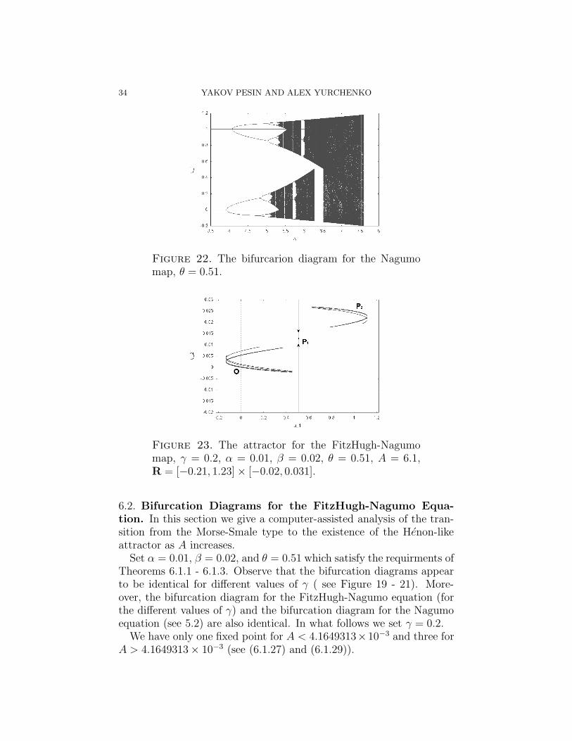
Figure 22. The bifurcarion diagram for the Nagumomap, θ = 0.51.

Figure 23. The attractor for the FitzHugh-Nagumomap, γ = 0.2, α = 0.01, β = 0.02, θ = 0.51, A = 6.1,R = [−0.21, 1.23]× [−0.02, 0.031].

6.2. Bifurcation Diagrams for the FitzHugh-Nagumo Equa-tion. In this section we give a computer-assisted analysis of the tran-sition from the Morse-Smale type to the existence of the Henon-likeattractor as A increases.

Set α = 0.01, β = 0.02, and θ = 0.51 which satisfy the requirments ofTheorems 6.1.1 - 6.1.3. Observe that the bifurcation diagrams appearto be identical for different values of γ ( see Figure 19 - 21). More-over, the bifurcation diagram for the FitzHugh-Nagumo equation (forthe different values of γ) and the bifurcation diagram for the Nagumoequation (see 5.2) are also identical. In what follows we set γ = 0.2.

We have only one fixed point for A < 4.1649313×10−3 and three forA > 4.1649313× 10−3 (see (6.1.27) and (6.1.29)).




It follows from Theorem 6.1.1 that for small values of A the systemis of Morse-Smale type. As A increases we observe two sequences ofperiod doubling bifurcations around A = 4. The first sequence arisesfrom O and the second one from P2. It follows from Theorem 6.1.2that for A between approximately 4 and 7.8 there is a trapping region(rectangle) R, containing all three fixed points, and an attractor insideR.

At first the attractor contains only finitely many attracting and hy-perbolic periodic points and their unstable manifolds. As A increasesthe period doubling goes on and, as we believe, ends up with twoFeigenbaum attractors (in general, these attractors appear for differentvalues of A), one around P2 and another one around O.


When A exceeds the value A = 6 two Henon-like attractors appeararound the same two fixed points, P2 and O (they may correspond todifferent values of A). In each of these attractors the unstable manifoldof the corresponding fixed point is dense The basins of attraction ofthese attractors are separated by the stable separatrix of the fixed pointP1 (see Figure 23).

For A ≈ 6.3 the unstable separatrix of the fixed point O interesectsthe stable separatrix of P1 and all orbits in R will go to the only Henon-like attractor around P2 (see Figure 24). This does not happen in thesymetric case, θ = 0.5.

As A increases even further (approximately above 6.5), the two at-tractors collide and the unstable separatrices of P2 and O are dense inthe resulting Henon-like attractor (see Figure 25).

It follows from Theorem 6.1.3 that for large values of A the systemhas a horseshoe.

Appendix . Preliminaries (see [15], [25], [23])

Consider a C1 diffeomorphism f : M →M of a compact smooth Rie-mannian manifold M . We denote by Ω(f) the set of all nonwanderingpoints and by Per(f) the set of periodic points of f .

Recall that a diffeomorphism (endomorphism) f is called a Morse-Smale diffeomorphism (endomorphism) if

(1) Ω(f) = Per(f);(2) every periodic point is hyperbolic;(3) the global (local) stable and unstable manifolds of periodic

points intersect transversally.

If a map f : Rd → Rd has∞ as a fixed point (repelling or attracting),

one can define the compactification map f : Sd → Sd by

f = P f P−1,

where P : Sd\N → Rd is the stereographic projection and N is theNorth Pole of Sd.

References

[1] V. S. Afraimovich, Ya. Pesin, Travelling Waves in Lattice Models of Multi-dimensional and Multi-component Media: I. General Hyperbolic Properties,Nonlinearity, 6 (1993), 429-455.

[2] V. S. Afraimovich, Ya. Pesin, A. Tempelman, Travelling Waves in Lattice Mod-els of Multidimensional and Multi-component Media: II. Ergodic Propertiesand Dimension, Chaos, 3 (1993), no. 2, 233-241.


[3] D. G. Aronson, H. F. Weinberger, Nonlinear Diffusion in Population Genetics,Combustion and Nerve Propagation, Lecture Notes in Mathematics, Springer-Verlag, vol. 446, 5-49 (1975).

[4] P. J. Blennerhassett, On the Generation of Waves by Wind, Philos. Trans.Roy. Soc. London Ser. A 298 (1980/81), no. 1441, 451-494.

[5] Bonhoeffer, Activation of Passive Iron as a Model for the Excitaion of Nerve,J. General Physiology, vol. 32 (1948), 69.

[6] J. Cronin, Mathematical Aspects of Hodgkin-Huxley Neural Theory, Cam-bridge UP (1987).

[7] M. C. Cross, P. C. Hohenberg, Pattern Formation Outside of Equilibrium,Reviews of Modern Physics, Vol. 65 (July 1993), No. 3, 851-113.

[8] I. R. Epstein, J. A. Pojman, An Introduction to Nonlinear Chemical Dynamics,Oxford UP (1998).

[9] R. A. Fisher, The Genetical Theory of Natural Selection, Oxford UniversityPress (1930).

[10] R. A. Fisher, The Advance of Advantageous Genes, Annual of Eugenics, v.7(1937), 355-369.

[11] R. FitzHugh, Impulses and Physiological Models of Nerve Membrane, Biophys-ical J., v.1 (1961), 445-466.

[12] R. FitzHugh, Biological Engineering, McGraw-Hill (1969), 1-85.[13] A. V. Gaponov-Grekov, M. I. Rabinovich, Nonlinearities in Action, Springer-

Verlag (1992).[14] A. L . Hodgkin, A. F. Huxley, A Quantitative Description of Membrane Cur-

rent and Its Application to Conduction and Excitation in Nerve, J. Physiology,v.117 (1952), 500-544.

[15] A. Katok, B. Hasselblatt, Introduction to the Modern Theory of DynamicalSystems, Cambridge University Press (1998).

[16] A. N. Kolmogorov, I. G. Petrovskii, N. S. Piskunov, A Study of the DiffusionEquation with Increase in the Amount of Substance, and Its Application to aBiological Problem in Selected Works of A. N. Kolmogorov, vol. 1, 242-270,Kluwer Academic Publishers (Appeared in Bull. Moscow Univ., Math. Mech.1:6, 1-26, 1937).

[17] K. Maginu, Reaction-Diffusion Equation Describing Morphogenesis. I. Wave-form Stability of Stationary Solutions in a One Dimensional Model, Mathe-matical Bioscience, vol. 27 (1975), 17-98.

[18] C. Marchioro, M. Pulvirenti, Mathematical Theory of Incompressible Nonvis-cous Fluids, Springer-Verlag (1994).

[19] N. Minorsky, Introduction to Non-linear Mechanics, J. W. Edwards (1947).[20] J. D. Murray, Mathematical Biology, Springer (1993).[21] J. Nagumo, S. Arimoto, S. Yoshizawa, An Active Pulse Transmission Line

Simulating Nerve Axon, Proceedings of the IRE, October 1962, 2061-2070.[22] J. Nagumo, S. Arimoto, S. Yoshizawa, Bistable Transmission Lines, IEEE

Trans., Circuit Theory, 12 (1965), 400-412.[23] Z. Nitecki, Differential Dynamics, The MIT Press (1971).[24] D. R. Orendovici, Ya. B. Pesin, Chaos in Traveling Waves of Lattice Systems

of Unbounded Media, Numerical methods for bifurcation problems and large-scale dynamical systems, 327-358, IMA Vol. Math. Appl., 119, Springer (2000).


[25] J. Palis, W. de Melo, Geometric Theory of Dynamical Systems, Springer-Verlag(1982).

[26] C. V. Pao, Nonlinear Parabolic and Elliptic Equations, Plenum Press (1992).[27] C. Rocsoreany, A. Georgescu, N. Giurgiteanu, The FitzHugh-Nagumo Model,

Kluwer Academic Publisher (2000).[28] K. Stewartson, J. T. Stuart, A Non-linear Instability Theory for a Wave System

in Plane Poiseuille flow, J. Fluid Mechanics, vol. 48 (1971), part 3, 529-545.[29] A. M. Turing, The Chemical Basis of Morphogenesis, Phil. Trans. Roy. Soc.

B, vol. 237 (1952), 5-72.[30] F. Verhulst, Nonlinear Differential Equations and Dynamical Systems,

Springer-Verlag, 1990.

Department of Mathematics, Pennsylvania State University, Uni-versity Park, State College, PA 16802

E-mail address : [email protected]

Schoolof Mathematics, Georgia Institute of Technology, Atlanta,GA 30332

E-mail address : [email protected]

some physical models of the reaction ... physical models of the reaction-diffusion equation and...

Documents