some practical issues in the design and analysis of...
TRANSCRIPT
SOME PRACTICAL ISSUES IN THE DESIGN AND ANALYSIS OF COMPUTER EXPERIMENTS
Ton\- Sahama
THIS THESIS IS PRESENTED IN FULFILMENT OF
THE REQUIREMENTS OF THE DEGREE OF
DOCTOR OF PHILOSOPHY
SCHOOL OF COMPUTER SCIENCE AND MATHEMATICS
FACULTY OF SCIENCE, ENGINEERING AND TECHNOLOGY
VICTORIA UNIVERSITY OF T E C H N O L O G Y
2003

FTS THESIS 519.57 SAH 30001007907837 Sahama, Tony Some practical issues in the design and analysis of computer experiments
a '

© Copyright 2003
by
Tonv Sahama
The author herelj>' grants to Victoria Universit>' of Technology
permission to reproduce and distribute copies of this thesis
document in \\4iole or in part.
11

Certificate of Originality
I hereb\' declare that this submission is nn' own work and that, to the best of
m>- knowledge and beUef, it contains no material previously pubUshed or written
by another person nor material which to a substantial extent has been accepted
for the award of any other degree or diploma of a universit\- or other institute of
higher learning, except where due acknowledgement is made in the text.
I also hereb>- declare that this thesis is written in accordance with the Uni-
versit\-'s Polic\' witli respect to the Use of Project Reports and Higher Degree
Theses.
T. Sahama
111

Abstract
Deterministic computer simulations of physical experiments are now common
techniques in science and engineering. Often, physical experiments are too time
consuming, expensi\'e or impossible to conduct. Complex computer models or
codes, rather than physical experiments lead to the stud>- of computer experi
ments, which are used to investigate man>' scientific phenomena of this nature.
A conrputer experiment consists of a number of runs of the computer code with
different input choices. The Design and Anal>-sis of Computer Experiments is a
rapidly growing technique in statistical experimental design.
This thesis investigates some practical issues in the Design and Analysis of
Computer experiments and attempts to answer some of the questions faced b>'
experimenters using computer experiments. In particular, the cjuestion of the
number of computer experiments and how tlie>- should be augmented is studied
and attention is gi\'en to when the response is a function over time.
In\-estigation of the appropriate sample size for computer experiments is un
dertaken using three fire models and one circuit simulation model for empirical
\-aH(lation. Detailed illustrations and some guidelines are given for the sample size
and an empirical relationship is established showing how the a\'erage prediction
error from a computer experiment is related to the sample size.
When tlie average prediction error following a computer experiment is too
large the question of how to augment the computer experiment is raised. Two
approaches are studied, e\'aluated and compared. The first approach invoh'es
adding one point at a time and choosing that point with the maximum predicted
\'ariance, \\4iile the second approach im'oh'es maximising the determinant of the
variarice-co\'ariaiice matrix of the prediction errors of a candidate set.
i\'

Rath(>r than just examining a whole series of practical cases, the machinery
of computer experiments is also used to stud>- computer experiments themseh'es.
The inputs of the model are the parameters of the Krigmg model as well as the
number of input runs while the output is a measure of the prediction error. This
study provides predictions of the average prediction error for a wide range of
computer models.
Many computer codes provide not just a univariate response but a trace of
responses at various values of a time parameter. A method for analysing such
computer experiments is proposed and illustrated.

Acknowledgements
• 1 wish to express my sincere gratitude to m>- supervisor. Dr. Neil Dia
mond, for his guidance, constructive criticism, \'aluable genuine ad\'ice and
encouragement given throughout the period of m>' Ph.D. stud>' at Victoria
University, Melbourne.
• I also wish to extend m>- deepest appreciation to Assoc. Prof. Neil Barnet.
former Head of the School, for providing me with a departmental scholarship
for the successful completion of this stud\-.
• Thanks are also rendered to Mr. P. Rajendran, Damon Burgess. Rowan
Macintosh and other colleagues who ha\'e been of immense assistance through
out this stu(l>'.
• I also would like to record m>- grateful thanks to Mr. Da\'id Abercrombie
and Mr. Ken Ling, School of Information S>-stems. Faculty of Information
Teclmology, Queensland Uni\'ersity of Technology for their encouragement
and support in numerous wa\'s.
• Special thanks to m\' wife Charlotte and our children Ishani and Ishara for
gi\-ing me all the support throughout my studies.
VI

Dedication
To my parents who taught me to work hard, to Charlotte who guided me to be
fair and stay curious, and to Ishani and Ishara for keeping me honest.
Vll

Preface
Parts of Chapters 3 and 4 appeared in Sahama and Diamond (2001).
Vl l l
Contents
1 Introduction 1
1.1 Computer Experiments 1
1.2 Role of Experimental Designs in DACE 3
1.3 Differences between Computer Experiments and Other Experimen
tal Design 3
1.4 Designs for Computer Experiments 5
1.5 Analysis of Computer Experiments 8
1.6 Thesis OutHne 15
2 Analysis of a Simple Computer Model 17
2.1 Introduction 17
2.2 Deterministic Fire Models 18
2.2.1 The ASET-B Fire Model 18
2.3 Experimental Design 21
2.3.1 Latin H>-perciibe Designs 21
2.3.2 Application to ASET-B Computer Experiment 22
2.4 Modelling 24
2.4.1 Summary of the Approach used by Sacks et al 24
2.4.2 Maximum Likelihood Estimation 24
2.4.-3 AppHcation to ASET-B Computer Experiment 28
2.5 Prediction 29
2.5.1 Prediction for Untried Inputs 29
2.5.2 Prediction Error 31
IX
2.5.3 Apphcation to ASET-B Computer Experiment 32
2.6 Interpretation of Results 32
2.6.1 Analysis of Main Effects and Interactions 32
2.6.2 Apphcation to ASET-B Computer Experiment 36
2.7 Conclusion 39
3 Sample Size Considerations 40
3.1 Introduction and Background 40
3.2 Some Details of the Selected Computer
Models 41
3.2.1 DETACT-QS 41
3.2.2 CIRC 42
3.2.3 DETACT-T2 43
3.3 Effect of Sample Size on ERMSE 45
3.3.1 Introduction 45
3.3.2 Methods 45
3.3.3 Results 46
3.4 Other Measures of Prediction Quality 46
3.5 Relationship between ERMSE and n 48
3.6 Discussion 49
4 Augmenting Computing Experiments 56
4.1 Introduction 56
4.2 Adding one run to a computer experiment 57
4.3 Adding more than one run to a computer experiment 59
4.4 Another Possible Approach 64
4.5 Discussion Go
5 A Model for Computer Models 68
5.1 Introduction 68
5.2 Simidating ASET-B 68
5.3 Design of the Exi^eriment 70

5.4 .A Computer Model Approach 80
5.5 Some Apphcations of the Results 83
5.6 Conclusions 83
6 Analysis of Time Traces 86
6.1 Introduction 86
6.2 Possible Methods 86
6.2.1 Separate Calculation for a Number of Time Points 88
6.2.2 Using Time as an Additional Input Factor 99
6.3 Conclusion 104
7 Discussion 105
7.1 Introduction 105
7.2 Limitations 107
7.2.1 Use of Latin Hypercube 107
7.2.2 Relationship between Sample Sizes and EMSE 107
7.2.3 Use of onh-Gaussian Product Correlation Structure . . . . 107
7.3 Future Work 107
7.3.1 AppHcation to other Designs 107
7.3.2 Application to other Computer Models 108
7.3.3 Prior Estimates of 9 and /; 108
7.3.4 Model Diagnostics for Time Trace Data 109
7.3.5 Multivariate Responses 109
Bibliography 110
xi
List of Tables
2.1 Input Variables for ASET-B Fire Model 24
2.2 Scaled LHD points for ASET-B Input Variables. [Runs 1 to 25
of .Y = 50] and corresponding Egress Times. Coding scheme:
scaled [—1,-1-1] input variables have been multiplied by 49. 25
2.3 Scaled LHD points for ASET-B Input Variables. [Runs 26 to 50
of N — 50] and corresponding Egress Times. Coding scheme:
scaled [—1.-1-1] input variables ha\-e been multipUed by 49 20
2.4 Some suggested \-alues for ^s and ps from selected cases 28
2.5 Estiniatc^s of ^i d_i from 10 Random Starts with one Maximum
(12.12207) 29
2.6 Estimates of py p^ from 10 Random Starts with one Maximum
(12.12207) 29
2.7 Estimates of ^j 64 from 10 Random Starts with Different Max
imum (MLE) 30
2.8 Estimates of p i , . . . ./ 4 from 10 Random Starts with Different Max
imum (MLE) 30
2.9 Estimates of Parameters for the ASET-B Computer Model 31
2.10 Functional ANOVA decomposition for the ASET-B experimental
data 39
3.1 Input Factors for DETACT-QS Computer Model 42
3.2 Minimum. Intermediate and Maximum le\-els of the controllable
factors for the CIRC Computer Model !•)
3.3 Manufacturing variations of the factors in the CIRC computer
Model 43
xii

3.4 Input Factors for D E T A C T - T 2 Computer Model 45
3.5 ERMSE for 3 LHDs for Sample Sizes of 10. 2 0 , . . . . 100 with the
ASET-B Computer Model 46
3.6 ERMSE for 3 LHDs for Sample Sizes of 10,20.... .100 with the
DETACT-QS Computer Model 47
3.7 ERMSE for 3 LHDs for Sample Sizes of 10,20,... .100 with the
CIRC Computer Model 48
3.8 ERMSE for 3 LHDs for Sample Sizes of 10,20,... .100 with the
DETACT-T2 Computer Model 49
3.9 Estimates of a, b and a 50
4.1 Coded design points of the Initial Design with Egress Times from
ASET-B 58
4.2 Results of Modelling ASET-B using the 20 run design gi^•en in
Table 4.1 59
4.3 Coded potential augmenting runs with Egress Times from ASET-B. 59
4.4 Ten Candidate Points following a Tweiit>' Points LHD for the
ASET-B Fire Model; and MSE of Prediction for the 1st. 2ii(l
5th added points 61
5.1 Results for experiment on surrogate ASET-B model 69
5.2 Runs 1 32 of the Box-Behnken experiment on the ASET-B Fire
Model 72
5.3 Runs 33 64 of the Box-Behnken experiment on the ASET-B Fire
Model 73
5.4 Runs 65 96 of the Box-Behnken experiment on the ASET-B Fire
Model 74
5.5 Runs 97 130 of the Box-Behnken experiment on the ASET-B Fire
Model 75
5.6 Results for the Box-Behnken design on the ASET-B Computer Model 77
6.1 Scaled LHD points for ASET-B Input Variables, [Runs 1 to 25 of
A- = 50] 89
xm
6.2 Scaled LHD points for ASET-B Input Wuiables. [Runs 26 to 50 of
A' = 50] 90
6.3 Scaled LHD points for ASET-B Input Variables. [Runs 1 to 25 of
A' = 50] and corresponding Egress Times from 0 to 30 seconds in
five second intervals 91
6.4 Scaled LHD points for ASET-B Input Variables, [Runs 26 to 50 of
A' = 50] and corresponding Egress Times from 0 to 30 seconds in
five second intervals 92
6.5 Scaled LHD points for ASET-B Input Variables, [Runs 1 to 25 of
A = 50] and corresponding Egress Times from 35 to 65 seconds in
five second intervals 93
6.6 Scaled LHD points for ASET-B Input Variables, [Runs 26 to 50 of
A' = 50] and corresponding Egress Times from 35 to 65 seconds in
five second intervals 94
6.7 Scaled LHD points for ASET-B Input Varial)les. [Runs 1 to 25 of
A' = 50] and corresponding Egress Times from 70 to 100 seconds
in five second intervals 95
6.8 Scaled LHD points for ASET-B Input Variables, [Runs 26 to 50 of
A' = 50] and corresponding Egress Times from 70 to 100 seconds
in five second intervals 96
6.9 Results of analysing Time Trace data using method 1 98
6.10 Predicted Response versus Actual response at five second time
inter^•als using method 2 102
xiv
List of Figures
2.1 Simple Illustration of ASET-B enclosure fire 20
2.2 Projection Properties of a LHD with 11 runs 23
2.3 Projection Properties of a LHD with 50 runs 27
2.4 Accuracy of Prediction for Egress Time 32
2.5 Main Effects plot for the ASET-B Computer Model 36
2.6 Interaction plot for the ASET-B Computer Model 37
2.7 Joint Effects for the ASET-B Computer Model 38
3.1 Diagram of Wheat stone Bridge 44
3.2 Scaled ERMSE \-ersus sample size for the four computer models. . 50
3.3 Rp versus sample size for the four computer models 51
3.4 Contour Plot of R^ v(>rsus Ai and A2 for ASET-B 52
3.5 Contour Plot of 7?2 versus Al and A2 for DETACT-QS 52
3.6 Contour Plot of 7? \-ersus Ai and A2 for CIRC 53
3.7 Contour Plot of 7?2 versus Al and A2 for DETACT-T2 54
3.8 Plots of Linear Relationship for Different Computer Models. . . . 54
4.1 Original 20 points from a LHD plus 10 labeled candidate points
from a 10 run LHD 60
4.2 Mean Square Error of Prediction adding one point at a time. . . . 62
4.3 Determinant of the variance-covariance matrix of predictions for
all possible run combinations of five runs from the candidate set
of 10 runs 64
5.1 Comparison of Simulation Of ASET-B with actual results 70
5.2 Main effects plots for the model of computer models 79
5.3 Joint effect plot of n and p for the model of computer models. . . 80
XV

5.4 Joint Effects of n and 6 for the model of computer models 81
5.5 Joint effect plot of 9 and p for a one-dimensional computer model. 82
5.6 Joint effect plot of 9i and p2 for the model of computer models. . 83
5.7 Joint effect plot of ^i and ^2 for the model of computer models. . 84
5.8 Joint effect plot of pi and p2 for the model of computer models. . 85
5.9 Comparison of results for ASET-B and predictions from the quadratic-
and marginal models 85
6.1 Generated Time Traces for the ASET-B Latin Hypercube Experi
ment 88
6.2 Estimated 9s for Time in 5 second intervals 97
6.3 Estimated ps for Time in 5 second intervals 99
6.4 Predicted Response versus Actual response at 5 second time inter
vals using; method 2 101
xvi
Chapter 1
Introduction
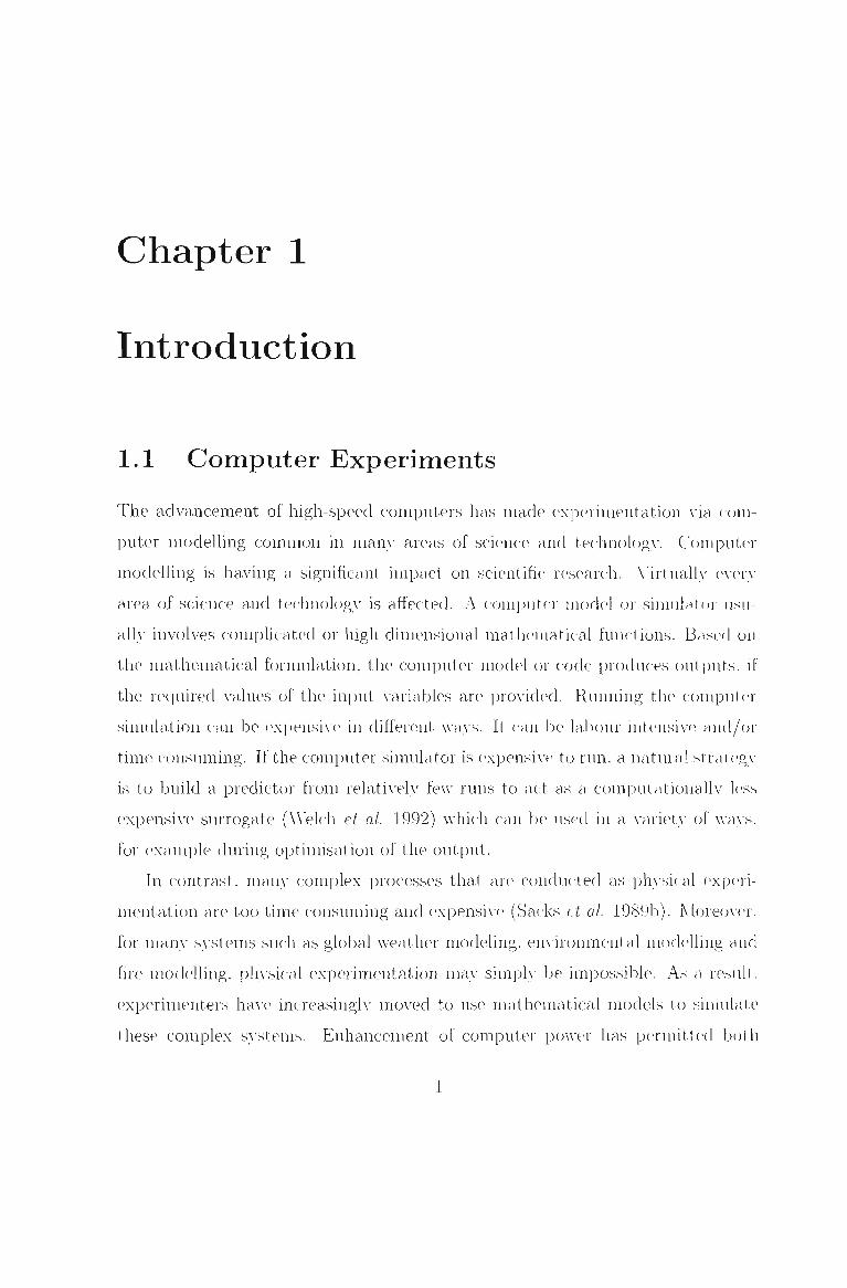
1.1 Computer Experiments
The advancement of high-speed computers has made experimentation \-ia com
puter modelling common in many areas of science and technolog>-. Computer
modelling is having a significant impact on scientific research. \'irtually e\er>-
a,rea. of science and technolog>' is affected. A computer model or simulator usu
ally involves complicated or high dimensional mathematical functions. Based on
the mathematical formulation, the computer model or code produces outputs, if
the reciuired \'alues of the input \'ariables are provided. Running the computer
simulation can be expensive in different wa>'s. It can be labour intensive and/or
time consuming. If the computer simulator is expensive to run, a natural straleg>'
is to build a predictor from relativeh- few runs to act as a computationally less
expensive surrogate (Welch et al. 1992) which can be used in a variety of waA's.
for example during optimisation of the output.
In contrast. man>' complex processes that are conducted as physical (experi
mentation are too time consuming and expensi\'e (Sacks et al. 1989b). Moreover,
for many s>-stems such as global weather modeling, en\-ironmental modelling and
fire modelling, physical experimentation may simply be impossible. As a result.
experimenters ha\'e increasing!}' moved to use mathematical models to simulate
these complex systems. Enhancement of computer power has permitted b(jth
1
CHAPTER 1. INTRODUCTION 2
greater complexity and more extensi\e use of such models m scientific experi
mentation as well as in industrial processes. Computer simulation is imariabl)'
cheaper than physical experimentation although these codes can be computation
ally demanding (Welch and Sacks, 1991).
This computer experiment approach has opened up a new avenue. "Design
and Analysis of Computer Experiments" (DACE), which is somewhat different
to the traditional methodology for the "Design of Experiments" (DoE). A signif
icant comparison between DACE and DoE concepts was presented b>' Booker ef
al. (1996). Booker (1996) compared DACE to DoE in three application areas:
electrical power system design, aeroelastic design and aerod\iiamic design. As
Booker suggested "DoE and DACE . . . [are basically] the same approach employ
ing different tools as appropriate''.
In general, computer models or codes consist of multivariate inputs. wJiich
can be scalars or functions (Sacks et al. 1989b) and th(> resulting output from
the same code may also be univariate and/or multivariate. In addition, the
output can be a time dependent function and the enhanced abiUt\- to gather and
analyse a number of summar\- responses \A-as highlighted by Sacks et al. (1989b).
The input dimension differs according to the purpose and basis of the original
computer model. Selecting a number of runs out of various input configurations
results in Computer Expenments.
One of the important application areas is the computer simulation of inte
grated circuits. Here (x) defines \'arious circuit parameters, such as transistor
cliaracteristics, and (y) is a measurement of the circuit performance, such as
output \'oltage. Tlie literature shows some other apphcations in a wide variety
of fields such as plant ecolog>- (Bartell et a.l., 1981 and 1983), Heat combustion
(Miller and Frenklach, 1983). chemometrics (Ho et al. 1984). controUed-nuclear-
fusion devic-es (Nassif et al, 1984). thermal-energy storage (Currin et al 1988),
VLSI-circuit design (Sharifzadeh et al, 1989). Solar CoUector Experiments and
Automotive Industr>- (Schonlau, 1997), Biomechanical Engineering (Chang et al
1999) and Oil liydrocarbon reservoir simulation (Graig et al. 1996) and (Kcnmech-
and OTIagan. 2000). Other apphcation areas, as highlighted in Koehler (1990).

CHAPTER 1. INTRODUCTION .]
wer(> a mold filling process for manufacturing automobiles, chemical kinetic mod
els, a thermal energy storage model and the transport of pol>x>'clic aromatic
hydrocarbon spills in streams using structured actiAit\- relationships model being
of use in plant ecolog\-. In fact, the widespread use of computer models and ex
periments for simulating real phenomena generates examples in \irtuall\- all areas
of science and engineering.
1.2 Role of Experimental Designs in DACE
Experimental design, as a statistical discipline, began with the pioneering work
of R.A. Fisher in the 1920s. It is one of the most powerful tools of statistics and
is widely used when designing experiments. Experimental designs have been used
to mitigate the effect of random noise in experimental outcomes. Howe\'er, the
ke>' ideas of randomisation, replication, and blocking are not useful for computer
experiments.
In contrast, the Design of Computer Experiments is a new a\'enue in the
Design of Experiments since there are no random errors. Also, replication is
not uecc^ssary since one always obtains the same response at the sam(> iiii)ut
settings (Booker 1996). The role of statistical experimental design in Computer
experiments was reviewed by Sacks et al (1989b), stating that . . . . " the selection
of inputs at which to run a computer code is still an ciperiniental design problem ".
1.3 Differences between Computer Experiments
and Other Experimental Design
AUhough Factorial and Fractional Factorial designs are most commonly used for
physical experiments, in computer experiments perhaps the most common designs
are Latin Hypcncube Designs (LHD). These were the first type of designs to be
explicitly- considered as experimental designs for deterministic computer codes.
Computer models are deterministic: rephcate observations from running the
CHAPTER 1. INTRODUCTION 4
code with the same inputs will be identical. Since these models have no ran
dom or measurement errors, computer experiments are different from physical
experiments calling for distinct techniques for design. These deterministic com
puter experiments differ substantially from the niajorit}' of ph>-sical experiments
traditionally performed by scientists. Such experiments usually haA-e substantial
random error due to variabihty in the experimental units (Sacks et al. 1989b).
The remarkable methodology of statistical design of experiments was intro
duced in the 1920's and popularised among scientists following the publication
of Fisher (1935). The associated analysis of variance is a systematic wa>- of sep
arating important treatment effects from the background noise (as well as from
each other). Fisher's methods of blocking, replication and randomization in these
experiments reduced the effect of random error, provided valid estimates of un
certainty and preserved the simplicit>' of the models. The deterministic computer
codes considered in this thesis differ from codes in the simulation literature (Sac ks
et al 1989b), which incorporate substantial random error through random num
ber generators. The random (as opposed to deterministic) simulation, i.e., com
puter models that use pseudorandom numbers (as in man>' telecommunications
and logistic applications) described by Law and Kelton (2000) is a significant
contribution for simulation experiments. It has been natural, therefore, to design
and anah'se such stochastic simulation experiments using standard techniques
for pliA'sical experiments. Howevcn'. it is doubtful whether these methods are ap
propriate for computer experiments considered here since the prediction wiU not
then inatcli the observed deterministic respomse. For this reason other methods
of design and anah'ses haA-e been de\-eloi)ed 1J\- a number of authors.
The design problem is the choice of inputs for efficient analysis of the data. A
c'omputer experimental design consists of a set of sample points to be evaluated
through the computer code or model. The observations from this design are tlieii
used to develop a computationally cheaper surrogate model to the code. This
n(>w model is used to estimate the code inexpensively and efficienth-. to iii\-es-
tigate the behavior of the function, or to optimise some aspect of the function.
••Computer e.rperiments are efficient methods of extracting information about the

CHAPTER 1. INTRODUCTION 5
unkrioIvn function and providing an approximating model that can be nif.rjMiisieelij
evaluated" (Koehler and Owen, 1996).
1.4 Designs for Computer Experiments
McKay et al. (1979), were the first to exphcitly consider experimental de
sign for deterministic computer codes. With the input variable giA-en 1)\- X =
(X^,... ,X^) where X^ is a standardised input between 0 and 1. and the output
produced by the computer code given by y = /^(X), they compared 3 methods of
selecting the input variables:
1. Random Sampling
2. Stratified Sampling
3. Latin Hypercube Sampling - an extension of stratified sampling which en
sures that each of the input \-ariables has all portions of its range repre
sented. A uniform Latin II\-percube sample of size n has
A7 = ^ ^ ^ ^ - ^ . l < ^ < n . l < . 7 < f / n
n. where 7rj(l) 'T"J('0 ^^6 random permutations of the integers 1,.
Uj '^U[0,1] and the d permutations and nd uniform variates are mutuall\'
independent (Owen. 1992a). Many authors use the simpler Lattice samijle.
following Patterson (1954), where
A7 = !l(!l_zi. l < ^ < n . l < ;<d. n
A slightly altered definition has been used in this thesis.
Latin H>-percube samples haA-e been used extensi\'el\-. Iman and Conover
(1980) ai)plied Latin Hypercube Sampling to a Ground Water Flow S>-stein where
it. was desired to consider the potential escape of radio nucleotides from a deposit
for radioacti\'e waste and their migration from the subsurface to the surface en
vironment. They also gave a generafisation of Latin Hypercube Sampling that

CHAPTER 1. INTRODUCTION 6
allowed for different assumptions on the input variable to be studied without ad
ditional computer runs. Iman and Conover (1982) showed how Latin H>-percube
Samples could be modified to incorporate the correlations that ma>- exist among
the input variables. The method was used on a model for the studA- of Geological
Disposal of Radioactive Waste. Stein (1987) ga\-e the asymptotic \'ariance of the
Latin Hypercube based estimation and showed that the estimate of the expected
value of a function based on a Latin H>-percube sample is asA'mptotically normal
and that the improvement over simple random sampling depends on the degree
of additivity of the function of the input variables. He also provided a better
method than Iman and Conover (1982), of producing Latin Hypercube sampling
when the input variables are dependent.
Other experimental designs based on different optimality criteria w-ere stud
ied by Koehler (1990) who considered Entropy. Mean Square Error. Minimax.
Maximin and Star-discrepanc\- based designs. In addition, three examples were
studied: one a chemical kinetics prolDlein involving 11 differential equations. The
second example investigated was a large linear s>-stem of differential ec(uations
involving methane combustion with s(>\-en rate constants regarded as inputs. To
reduce the computer time, the design is restricted to a central composite design
t.\-i:)e (Box and Draper, 1987) but witli unknown shrinkage factors for the cube
points and the star points of the design.
A number of computational methods for augmenting the design were described
which would be classified as single stage methods, sequential methods without
adaptation to the data, and seciuential methods with adaptation. The problem
of how to design an augmenting experiment is an important one. It is clear,
hoAvever. tliat much more work needs to be done to make these methods easier
to use and this is something this research stud>- aims to accomplish.
Owen (1992b) generalised Latin H\-percube samples bv using orthogonal ar-
raA's (RaghaA-arao, 1971). An orthogonal arra>- of strength t is a matrix of n ro\\-s
and k columns with elements taken from a set of q SA-mbols such that in an>- n by
/ matrix each of the q^ possible rows occurs the same number A of times. Such
an array is denoted by OA{n.k.q,t). A generalisation of the Latin Hypercube

CHAPTER 1. INTRODUCTION 7
sample is giA-en b>'
.X; = i M i l i l . 0 < , < 1 , 0 < ; < - 1 Q
where the TTJ are independent permutations of 0 ,q — I and .4^ is the Aalue of
the i'^ row and j ^ ' ' column of an orthogonal arra>-. Similarl>-. Lattice samples can
be generalised b>' taking
Owen (1992b) suggests that the arrays OA{q'^. k, q, 2) are a good choice for com
puter experiments since the n = q^ points plot as a g x g grid on each bivariate
margin. He also presents OA of strength 2 of the form OA {q^.q + Lg,2) for
q = 2,3.4,5,7,8,9,11.13,16,17,19,25,27. and 32 and OA {2q^,2q ^-l.q,2) for
q = 2,3,4,5,7,8,9,11,13,16 although the latter designs include the same pro
jections in three columns that include repeat runs, an undesirable feature for a
computer experiment. In a later paper, (Owen 1994b), it is conjectured that
sub-arrays of the form OA {2q^.2q.q. 2) do not have this defect.
Owen (1992a) also suggests wa>-s to augment a computer experiment. If an
experiment based on an OA {q. d. q. 1) has been run then it can be used as an
angnienting set for those runs that would complete an OA {2q. d. q. 1). If we want
to increase the number of \-arial)les then OA {q^. d. q. 2) x OA (g^, (P, cf. 1) could
be used.
Independent to the work of Owcni. Tang (1993) also generalised Latin lly-
j)ercul)es b>- developing Orthogonal ArraA- based Latin Hypercube Designs. OA
based Latin Hypercubes offers a substantial improvement over Latin H>-per(ube
sampling and are proposed to be a more appropriate design for Computer Exper
iments.
Booker (1996) compared two experimental designs naiiielv Central Composite
Designs lor DoE and Space-FiUing Designs for DACE apphcations. According to
Booker, Latin H\-percube samples are one class of quasi-Monte Carlo iiitc^gration
designs based on random assignments that are generalh- ineffective for large prob
lems. Booker suggested that the possibihty of using Orthogonal Arrays (OA) as
CHAPTER 1. INTRODUCTION 8
an experimental design to be used in Computer Experiments for DACE would
gi\-( more confidence because of its good space-filling properties and infiltration
of the design space. He gaA-e examples A\-here he had used OA-based Latin H\--
percube samples which are derived from OAs, for an areoelastic simulation of the
performance of a helicopter rotor.
1.5 Analysis of Computer Experiments
In a computer experiment, observations are made on a response function y b\-
running a (typically complex) computer model at \^arious choices of input factors
X. For example, in the chemical kinetics of methane combustion, x can be a set of
rate constants in a system of differential equations and y can he a concentration of
a chemical species some time after combustion. Soh-ing the differential equations
numerically for specified x >-ields a value for y. Because running the equations
soh'er is expensive, the aim is to estimate the relationship between x and y from
a moderate number of runs so that y can be predicted at untried inputs.
Extracting observations from this design can be used to build up a computa-
tionalh- inexpensive surrogate model to the selected simulator or coni])uter code.
This surrogate model is used to approximate the computer simulator or model
cheaply and efficientl>-. to iin'estigatt^ the behaviour of the function and/or to
optimise some aspect of the function.
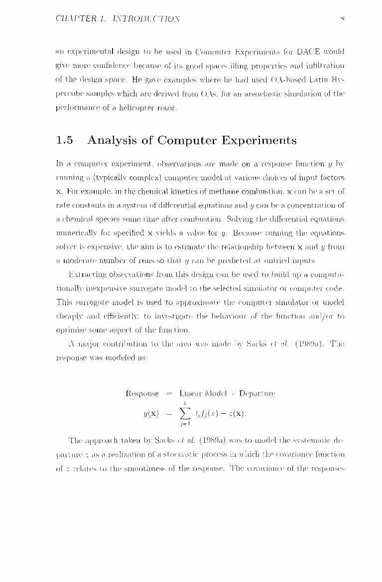
A major contribution to the area was made by Sacls;s et al. (1989a). The
response \\-as modeled as:
Response = Linear Model -I- Departure k
yW = 5].i,/,(x) + z(x).
The approach taken b.A- Sacks et al. (1989a) was to model the s\steiiiatic dc>-
parture z as a realization of a stochastic process in which the ccn-axiance function
of z r(4ates to the smoothness of the response. The ccn-ariance of the responses
CHAPTER 1. INTRODUCTION 9
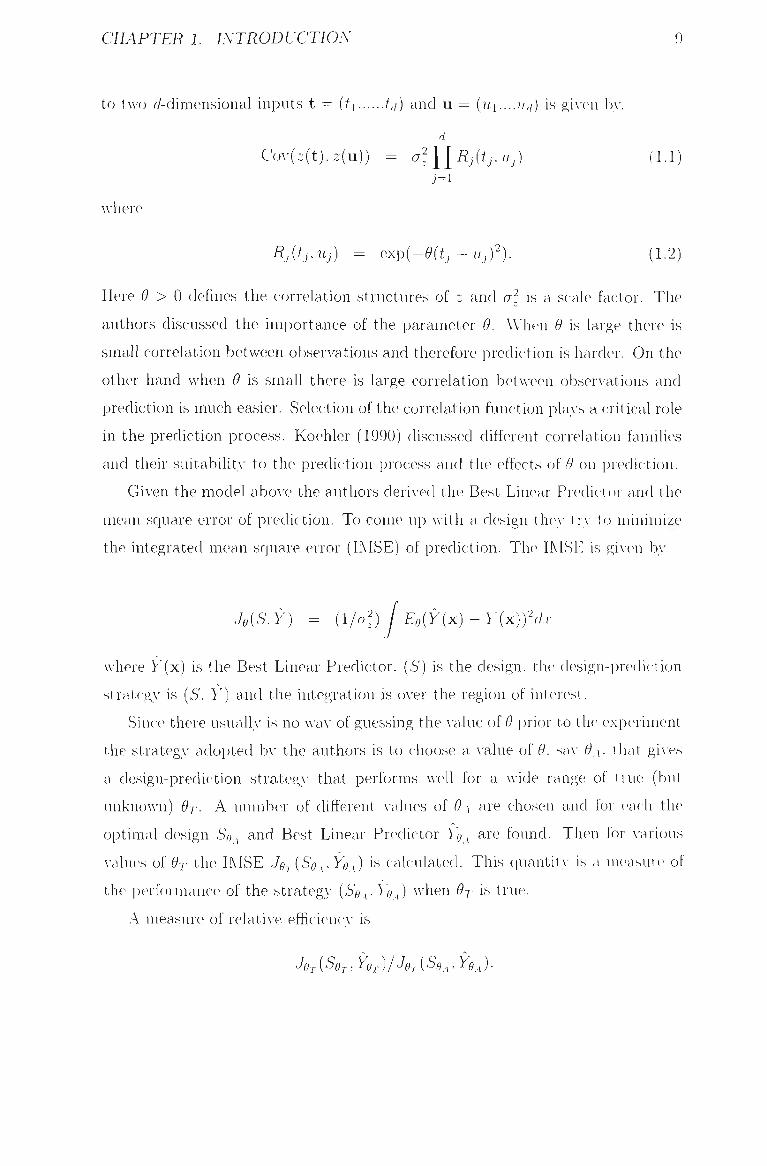
to two r/-dimensional inputs t = (ti /,/) and u = {ui....)i,i) is given by.
d
Coy{z{t).z{u)) = alY[Rj{t^.Uj) (1.1)
i=i
where
Rjilj.uj) = exp{-9{t,-u,)'). (1.2)
Here ^ > 0 defines the correlation structures of z and cx is a scale factor. The
authors discussed the importance of the parameter 6. When 9 is large there is
small correlation between observations and therefore prediction is harder. On the
other hand when 9 is small there is large correlation between observations and
prediction is much easier. Selection of the correlation function plaA-s a critical role
in the prediction process. Koehler (1990) discussed different correlation families
and their suitabilit.\- to the prediction process and the effects of 9 on prediction.
Given the model above the authors deriA-ecl the Best Linear Predictor and the
mean square error of prediction. To come up with a design the>- tr>- to minimize
the integrated mean square error (EMSE) of prediction. The IMSE is given by
JeiS.Y) = [llaD j Ee{Y{yi)-Y{^))hlx
where V'(x) is the Best Linear Predictor, (5) is the design, the design-prediction
strategA' is {S. Y) and the integration is OAer the region of interest.
Since there usualh' is no AvaA- of guessing the A alue of 9 prior to the experiment
the strategy adopted bA- the authors is to choose a A alue of 9. sav 9\. that gi\-es
a design-prediction strategA- that performs well for a A\-ide range of true (but
unknown) 9T- A number of different values of 9\ are chosen and for each the
optimal design SQ^ and Best Linear Predictor Yg^ are found. Then for various
A'alu(\s of 9T the IMSE Jej.{Se^^.Ye^) is calculated. This quantitA' is a measure of
the ])(nforiiiance of the strategy [SQ^, YQ /) when 9^ is true.
A measure of relative efficiencA- is
JOT ( er 1 ^dr ) I JBT WB.A- ^9A ) •
CHAPTER 1. INTRODUCTION 10
A robust strategy is to choose 9A SO that these relatiA-e efficiencies are as ( onstaiit
as pos,sil)le.
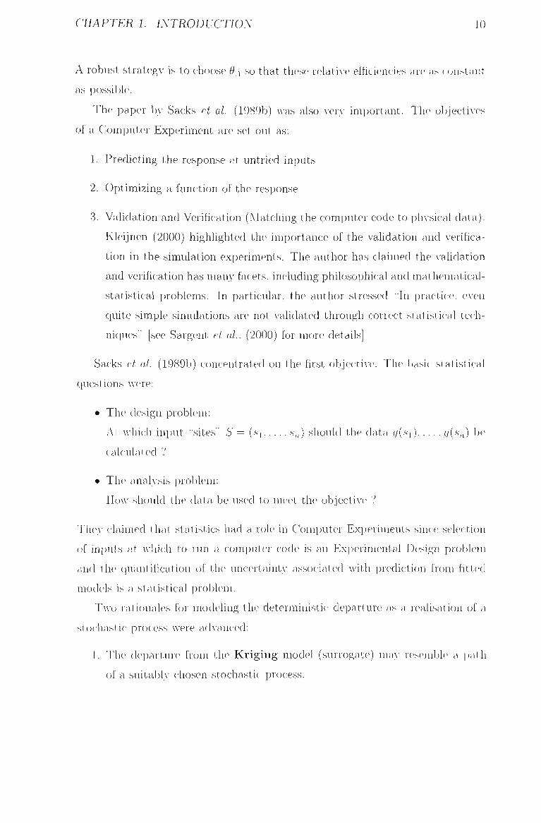
The paper In- Sacks et al (1989b) Avas also very important. The objectiA-es
of a Computer Experiment are set out as:
1. Predicting the response at untried inputs
2. Optimizing a function of the response
3. Validation and Verification (Matching the computer code to physical data).
Kleijnen (2000) highlighted the importance of the A^alidation and verifica
tion in the simulation experiments. The author has claimed the A^alidation
and verification has many facets, including philosophical and mathematical-
statistical problems. In particular, the author stressed "In praetice, even
ciuite simple simulations are not validated through correct statistical tech-
nic|ues" [see Sargent et al, (2000) for more details]
Sacks et al (1989b) concentrated on the first objectiA-e. The basic statistical
ciuestions Avere:
• The design problem:
At which input "sites" S = ( s i , . . . , .s„) should the data y{sy)..... y{sn) be
calculated ?
• The anal\-sis problem:
HoAv should the data be used to meet the objectiA-e '.''
They c laimed that statistics had a role in Computer Experiments since selection
of inputs at \\-hich to run a computer code is an Ex]>erimental Design problem
and the quantification of the uncertaintA- associated with prediction from fitted
models is a statistical problem.
TAVC) rationales for modeling the deterministic departure as a realisation of a
stochastic process Avere adA-anced:
1. The departure from the Kr ig ing model (surrogate) maA- resemble a i)ath
of a suitably chosen stochastic process.
CHAPTER 1. INTRODUCTION 11
Kriging
Kriging is named after the South-African mining engineer D.G. Krige. It is
an interpolation method that predicts unknown A'alues of random function
or random process (Cressie, 1993). More precisely, a Kriging prediction is
a weighted linear combination of all output values already obserA^ed. These
weights depend on the distances betAveen the location to be predicted and
the locations already observed. Kriging assumes that the closer the in
put data are, the more positively correlated the prediction errors are. This
assumption is modeled through the correlogram or the related variogram.
Kriging is popular in deterministic simulation. Compared AA-ith linear re
gression analysis, Kriging has an important adA-antage in deterministic sim
ulation: Kriging is an exact interpolator: that is. predicted A-alues at ob
served input values are exactlA- eciual to the obserA^ed (simulated) output
values [Kleijnen and A an Beers (2003)].
2. y(.) may be regarded as a Bayesian prior on the true response function,
Avith the 'Ts either specified a priori or given.
The Best Linear Predictor Estimate^ (Welch et al. 1992) Avas USCHI - this is
related to the concept of Krigmg in the Geostatistical literature (Cr(\ssie, 1986).
Alternativeh- the posterior mean could be used from a Bayesian A-ieAV]3oint.
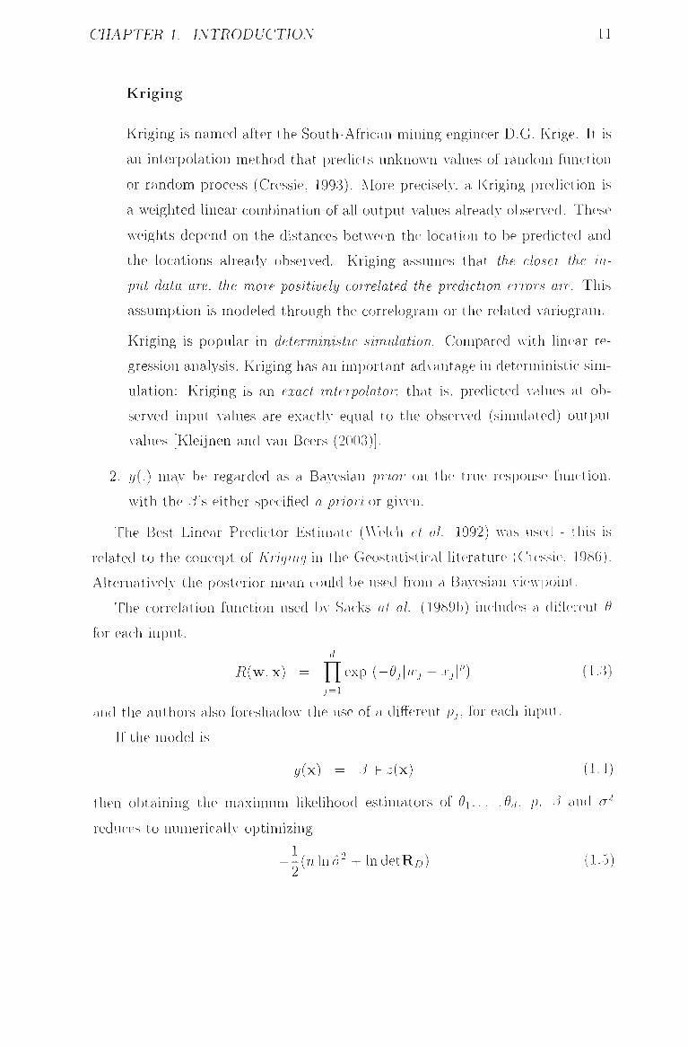
The correlation function used f)>- Sacks al al. (1989b) includes a different 9
for each input, d
7?(w.x) = llexp {-9,\w, - x,\n (1.3)
j = i
and the authors also foreshadoAA- the use of a different pj, for each input.
If the model is
y(x) = ,.3 + z(x) (1.4)
then obtaining the maximum likefihood estimators of 9i,....9d, p. p and a^
reduces to numericallA- optimizing I
- - ( n l n a ^ - h l n d e t R o ) (L5)
CHAPTER 1. INTRODUCTION 12
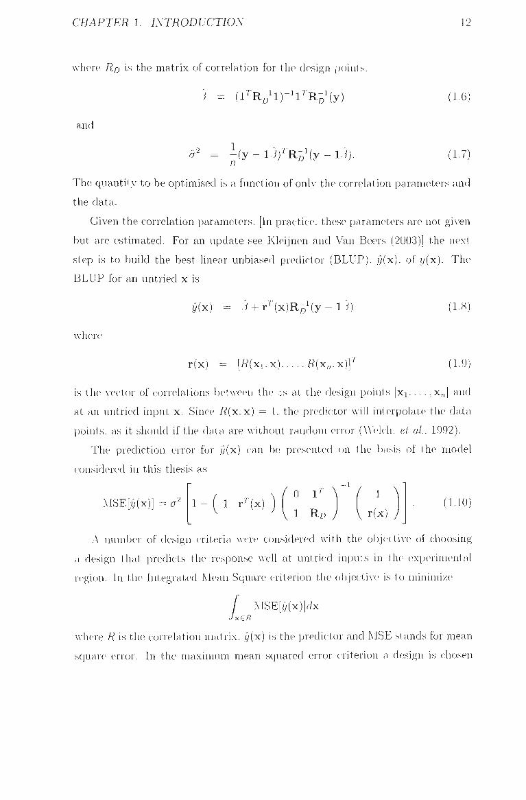
where RD is the matrix of correlation for the design points.
3 = ( l ^ R B ^ l ) - ^ l ^ R - i ( y ) (1.6)
and
a 2 1
iy-13fR^'(y-lJ}. (1.7) n
The quantity to be optimised is a function of only the correlation parameters and
the data.
Given the correlation parameters, [In practice, these parameters are not giA en
but are estimated. For an update see Kleijnen and Van Beers (2003)] the next
step is to build the best linear unbiased predictor (BLUP), y(x). of y(x). The
BLUP for an untried x is
y(x) = J + r^i^H^iy-lJ) (1.8)
A\4iere
r(x) = [i?(xi,x) R{^n.^)V (1-9)
is the A-ector of correlations Ijetween the ;s at the design points [xi . . . . ,x„] and
at an untried input x. Since /?(x, x) = 1, the predictor Avill interpolate the data
points, as it should if the data are Avithout random error (Welch, et al. 1992).
The prediction error for y(x) can be presented on the basis of the model
considered in this thesis as -1
MSE[y(x)] = a 2 1 - 1 r^(x T.IO)
A numbcn- of design criteria were considered \A-ith the objectiA'c of choosing
a design that predicts the response AA-CII at untried inputs in the experimental
region. In the Integrated Mean Square criterion the objective is to minimize
/ MSE[y(x)]f/x JxER
where R is the correlation matrix, y(x) is the predictor and MSE stands for mean
square error. In the maximum mean squared error criterion a design is chosen
CHAPTER 1. INTRODUCTION 13
to minimise the maximum MSE although this is much more computationally de
manding. A third criterion is the maximization of expected posterior entropy
(amount of information aA-ailable to the giA'en experimental region). The asymp
totic connection betAA een the maximization of expected posterior eiitrop\- criteria
(as est,al)lished by Johnson et al, 1990) is the need to in.sure that the design
will be effective even if the response A-ariable is sensitiA-e to only a fcAv design
variables. The goal of this is to find designs which offer a compromise between
the entroi)y maximin criterion, and projectiA-e properties in each dimension of
the response variable (Morris and MitcheU, 1995). An approach In- Ye et al,
(2000) on such "compromise between computing effort and design optimalitA-"" is
a significant improvement on constructing designs for computer experiment. The
authors claimed that the proposed class of designs [Symmetric Latin h}'percube
Design (SLHDs)] has some advantages over the regular LHDs AA-ith respect
to criteria such as entropA' and minimum intersite distance. The authors also
claimed that SLHDs are a good subset of LHDs witli respect to both entropy and
maximin distance criteria (for a comprehensi\-e discussion see Ye et al, 2000).
A number of interesting points A\-er( mack> in the discussion of the paper bv
Sacks et al. (1989b). Some of the discussants raised the possibility of using
factorial or fractional factorial design as cheap and simple designs that are nearh-
optimal in maiiA- cases. In their repl,\- the authors made the claim that suitablA-
scaled half fractions are apparentl>- optimal or close to optimal for the IMSE
criterion for the model Avith onl>- a constant term for the regressicm and p = 2. A
number of the discussants also examined the correlation function and stochastic-
process models and caUed for additional work in this area.
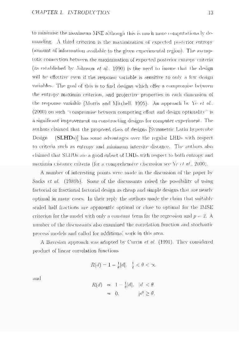
A BaA-esian approach was adopted by Currin et al (1991). They considered
product of linear correlation functions
R^d) = I - j\d\. 4 < ^ < o c
and R{d) = l - | | c i | , | r / | < ^
= 0, |r/| > e.
CHAPTER 1. INTRODUCTION 14
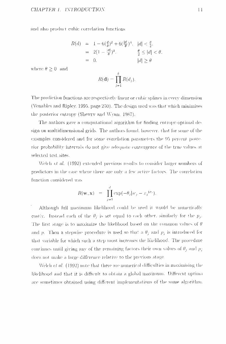
and also product cubic correlation functions
Rid) = l - 6 ( f ) 2 + 6(M)3. \d\<l,
= 2 ( l - ^ ) ^ f<ici|<^,
= 0, \d\ > 9
where ^ > 0 and k
R{d) = l[R{d,).
The prediction functions are respectiveh- hnear or cubic splines in e\-erA- dimension
(Venables and Ripley, 1995, page 250). The design used Avas that Avhich minimises
the posterior entropy (SheAvry and Wynn, 1987).
The authors gave a computational algorithm for finding entropA--optimal de
sign on multidimensional grids. The authors found. hoAvcA-er, that for some of the
examples considered and for some correlation parameters the 95 pcncent poste
rior probabilitA' intervals do not giA-e aclec[uate com^ergence of the true A-alues at
selected test sites.
Welch et al (1992) extended prcAdous results to consider larger numbers of
predictors in the case where there are OUIA' a feAv actiA-c- factors. The correlation
function considered was
/2(w,x) == lleM-9,\ir,-.r,n. j = i
Although full maximum likelihood could be used it Avould be numericallA-
costlA-. Instead each of the 9j is set equal to each other, similarly for the pj.
The first stage is to maximize the likelihood based on the common A-alues of 9
and p. Then a stepAvise procedure is used so that a 9j and Pj is introduced for
that A-ariable for Avhich such a step most increases the likelihood. The procedure
continues until giA'ing am- of the remaining factors their OAvn values of 9j and j)j
does not make a large difference relatiA-e to the previous stage.
Welch et al. (1992) note that there are numerical difficulties in maximising the
likelihood and that it is difficult to obtain a global maximum. Different optima
are sometimes obtained using different implementations of the same algorithm.

CHAPTER 1. INTRODUCTION 15
Good starting Aalues are also obviously an important part of the MLE calculation.
There is \-ery little hterature on how to get good starting values. One exception
is Owen (1994a) AVIIO gaA e a method for estimating 9i... . ,9^ AAhen p = I Avhich
could be used as starting A-alues in the maximum likelihood estimation.
A number of examples were presented In- Welch et al. (1992). For one example
involving only two A^ariables a 50 run Latin HA-percube Avas shoAvn to giA-e good
results. However, a 30 run and 40 run design does not identify a reasonable
model. No guidelines for the appropriate sample size are giA'en. In the second
example a 50 run Latin Hypercube Avas successful in identifying fiA-e significant
factors. The number of runs required for a computer experiment remains a kcA'
open question and is one that this research aims to tackle.
1.6 Thesis Outline
The thesis consists of seven chapters. The first chapter is a general introduction
and Literature RcA-iew of the area of computer experiments.
In the second chapter a simple computer model Avill bc introduced for the
purpose of describing exacth- Avhat a computer model is. hoAv it can be USCHI and
Avhat problems Avill be addressed in the thesis. The approach of modeling the
deterministic model as a stochastic process \\-ill be described. Focus Avill be on
important practical issues that haA e not receiA-ecl much attention in the literature
such as starting A-alues, parameterization and generating plots for interprc-tation.
The third chapter Avill focus on the effect of sample size (the number of com
puter experiments) on the precision of the predictions based on the fitted stochas
tic model, particularlA- in the case Avhen a Latin HA-percube design is used.
The fourth chapter Avill examine hoAv to add extra runs to a computer experi
ment in order to improve the precision of t he predictions. TAVO approaches Avill be
examined, one adding one point at a time Avhile the other adds groups of points
at a time.
In the fift h chapter a UCAV approach to addressing some of the issues of com
puter experiments Avill be developed. In this approach the structure of computer

CHAPTER 1. INTRODUCTION 16
experiments is used to stud\' computer experiments themseh-es. This is likelA' to
give results that are more general than the specific results deA'eloped in Chapters
3 and 4.
Many computer models giA-e the response as a function of time. HoAveAer most
of the literature on computer experiments focused on each run of the code giAdng
one response value. In Chapter 6 methods will be deA-eloped to efficientlA- analyse
the multivariate data generated by a computer code.
Finally Chapter 7 will give a discussion of the results and point out areas for
more research.

Chapter 2
Analysis of a Simple Computer
Model
2.1 Introduction
Since this thesis focuses on a number of ])ractical issues relating to the design
and analA'sis of computer experiments, it is of xalue here to descrilx* one model
in detail. This material Avill be used in later chapters. The particular (^xample
selected is A\-ailable Safe Egress Time (ASET-B), a computer model predicting
the nature of a fire in a single room, presented l)y Walton (1985).
A Latin Hyi)ercube Design (LHD) is used to choose input factors for the
ASET-B program. Based on this LHD, responses (y) from the model are gener
ated to form a computer experiment. The responses are modeled as thc> realisa
tion of a stochastic process, folloAving the AA'ork of Sacks et al. (1989a). Maximum
Likelihood Estimates (MLE) of the parameters are generated and these estimates
used to make predictions at untried inputs. The prediction can be made using
the Best Linear Unbiased Predictor (BLUP), a methodology introduced by Hen
derson (1975b) and Goldberger (1962). A graphical interpretation of the results
is presented.
17

CHAPTER 2. ANALYSIS OF A SIMPLE COMPUTER MODEL 18
2.2 Deterministic Fire Models
A stochastic process involves chance or uncertaintA-. In a deterministic \A'orld
everything is assumed certain. Deterministic fire models attempt to represent
mathematically the processes occurring in a compartment fire based on the laAvs
of physics and chemistry. These models are also referred to as room fire models,
computer fire models, or mathematical fire models. Ideally, tliCA- are such that
discrete changes in any physical parameter can be evaluated in terms of the effect
on fire hazard. While no such ideal exists in practice, a number of computer
models are available that provide a reasonable amount of selected fire effects
(Cooper and Forney, 1990).
Computer models have been used for some time in the design and analysis
of fire protection hardware. The use of computer models, commonly knoAvn as
design programs, has become the industry's standard method for designing \A-ater
supply and automated sprinkler SA-stems. These programs perform a large number
of tedious and lengtln- calculations and provide the user Avith accurate, cost-
optimised designs in a fraction of the time that AA-ould be rec|uired for manual
procedures.
In addition to the design of fire protection hardw-are, computer models nuu-
also be used to help CA-aluate the effects of fire on both people and propertA'. fhe
models can provide a fast and more accurate estimate of the impact of a fire
and help establish the measures needed to prcA-ent or control it. Wliile manual
calculation methods provide good estimates of specific fire effects (eg., prediction
of time to flash OA er), they are not well suited for comprehensive aiial\-sis iuA-oh'-
ing the time-dependent interactions of multiple physical and chemical processes
prc\sent in developing fires.
2.2.1 The ASET-B Fire Model
A-el-Fire is a complex phenomenon and a number of computer models have been cle
oped that reflect this complexitv-, for use IDA- scientists and engineers. One of tli
earliest models was the ASET (Available Safe Egress Time) mathematical mode

CHAPTER 2. ANALYSIS OF A SIMPLE COMPUTER MODEL 19
Avritten in FORTRAN by Cooper (1980). Later, Walton (1985) implemented the
model in Basic as ASET-B incorporating simpler numerical techniques to sohe
the differential equations involved.
ASET-B is a personal computer program for predicting the fire emironment
in a single room enclosure Avith all doors, Avindows and A-ents closed except for
a small leak at floor level. This leak preAents the pressure from increasing in
the room. A fire starts at some point below the ceihng and releases energy and
the products of combustion. The rate at Avhich these are released is likely to
change Avith time. The hot products of combustion form a plume Avhich, due to
bu(j>-ancy, rises. As it does so, it draAvs in to the room cool air Avhich decreases
the plume's temperature and increases its A'olume fioAv rate. Wlien the plume
reaches the ceiling it spreads out and forms a hot gas laA-er \A-hich descends \A-ith
time as the plume's gases continue to floAv into it. There is a relatiA-(4A- sharp
interface betAveen the hot upper laA-er and the air in the loAver part of the room
which, in the ASET-B model, is considered to be at ambient tempcTature. The
only interchange betAveen the air in the loAver part of the room and the hot upper
layer is through the plume.
ASET-B SOIA'CS scA-eral differential equations using a simpler numerical tech
nique than in the original ASET program. ASET-B requires as inputs the height
and area of the room, the elevation of the fire aboA-e the floor, a heat loss factor
(the fraction of the heat released b}- the fire that is lost to the bounding surfaces
of the enclosure) and a fire specified in terms of heat release rate w-hich depends
on the nature of the combustion material. For this study I ha\e used the ratc> of
release for a 'semi-uniA-ersal fire", corresponding to a "fuel package consisting of a
polyurethane mattress with sheets, fuels similar to AAood cribs and polyurethane
on pallets, and commodities in paper cartons stacked on paUets"' (Birk 1991, page
86). The program predicts the thickness and the temperature of the hot smoke
hiA-er as a function of time. A simple illustration of fire-in-enclosure floAv clA-iiam-
ics for an "uiiA-ented'" enclosure and the basic fire phenomena are presented in
Figure 2.1.
The response (y) was taken as the time it takes for the height of the smoke
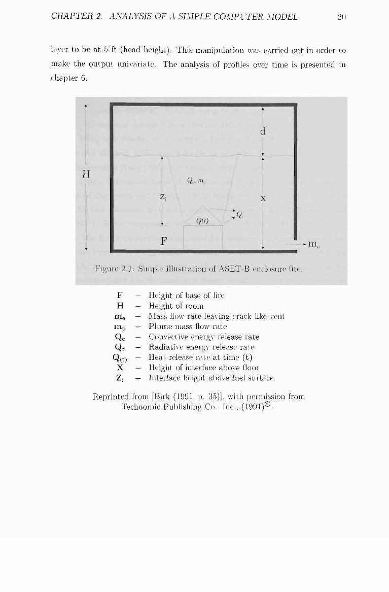
CHAPTER 2. ANALYSIS OF A SIMPLE COMPUTER MODEL 20
la\-c>r to be at 5 ft (head height). This manipulation was carried out in order to
make the output uniA-ariate. The analysis of profiles OA'er time is presented in
chapter 6.
F — Height of base of fire H — Height of room
nie — IMass AOAA- rate leaA-ing crack like \-eiit nip — Plume mass floAv rate Qc — Convective energA" release rate Qr — RadiatiA-e energA- release rate
Q(t) — Heat release rate at time (t) X — Height of interface aboA e floor Zi — Interface height aboA e fuel surface.
Reprinted from [Birk (1991. p. 35)], with permission frc m Technomic Publishing Co.. Inc., (1991)®.
CHAPTER 2. ANALYSIS OF A SIMPLE COMPUTER MODEL 21
2.3 Experimental Design
2.3.1 Latin Hypercube Designs
There are many experimental designs available for computer experiments. These
designs include the folloAving: Random Latin Hypercubes [McKa.A-. et al 1979],
Random Orthogonal Arrays (Owen, 1992b), IMSE Optimal Latin Ilvpercubes
(Park, 1994) and (Sacks, et al 1989b), Maximin Latin Hypercubes [MmLh]
(Morris and MitcheU, 1995) and (Johnson, et al 1990), OrthogonaUArrav based
Latin Hypercubes [Tang (1993) and Owen, (1992b)], Uniform Designs (Fang and
Wang, 1994), Orthogonal Latin Hypercubes (Ye 1998), Hammersley Sequence
Designs (Kalagnanam and Diwekar, 1997), Symmetric Latin Hypercubes (Ye et
al 2000) and Minimum Bias Latin Hypercube Design [MBLHD] (Palmer and
Tsui, 2001). Some comparisons were presented by Koeler (1990) and Simpson
(1998). The first experimental design used for computer experiments Avas a Ran
dom Latin Hypercube Design (LHD). discussed by McKay et al. (1979). A Latin
hypercube is a matrix of n roAvs and k columns where n is the number of IcA els
being examined and A- is the number of design A-ariables. Eac h column contains
the leA-c4s 1. 2 . . . . . n. randomly permuted, and the k columns are matched at
random to form the Latin liv])ercube. By their nature, Latin hA-])ercubes are
quite easA- to generate because thcA' require onh- a random permutation of n lev
els in each column of the design matrix. The big adA-antage of Latin hypercube
designs is that they ensure stratified sampling, i.e., each of the ini)ut A-ariables is
sampled at ?? IcA els. Thus. AA-hen a Latin h\-percube is projected or collapsed into
a single dimension, n distinct IcA els are obtained. This is extremely beneficial
for deterministic computer experiments since the Latin h\-percube points do not
oA-erlay). minimizing ariA- information loss. The main attraction of these designs
is that they ha\-e good one-dimensional projective properties Avhich ensure that
there is little redundanc.A^ of design points when some of the factors lia\-e a rel-
atiA-eh- negligible effect, called effect sparsity (Butler. 2001). "The use of Latin
li>-])erciibes does not put any serious restrictions on the applicabilitA- of the im
portance sampUng methods and the benefits of Latin hypercubes can be added to
CHAPTER 2. ANALYSIS OF A SIMPLE COMPUTER MODEL 22
the benefits of elaboratc> and efficient importance sampfing strategies. Therefore.
Latin liA-percube sampling has the qualifications to become a widelA- emploA-ed
tool in rehabihty analysis." (Olsson et al. 2003).
A LHD gives an evenlA- distributed projection into each of the input factors.
With this choice in a sample of size W the / '* obserA-ation for the /"" \-ariable is
given as
^j / M a x , - M i n A / M i n , + MaxA . ^ , . ^ ^.
'- = [ 2 )''-'[ 2 ) ' = l-----^/^^ = l -
where Max, is the Maximum of X,. Min, is the Minimum of X,-,
, _ 2 ^ , ( z ) - W - l r: N-V
and 7Tj{i) is the j " * obseiA-ation of a random permutation of the integers 1 , . . . . A'.
7r(j) = (7rj(l),. . . , 7rj{N)) and the d random permutations 7r ( l ) , . . . . 7r(d) corre
sponding to the d input factors are mutually independent. Note that —1 to 1 has
been chosen as the range for the coded in])uf factors, .r,, although some authors
(Sacks et al. 1989b) prefer a range of 0 to 1.
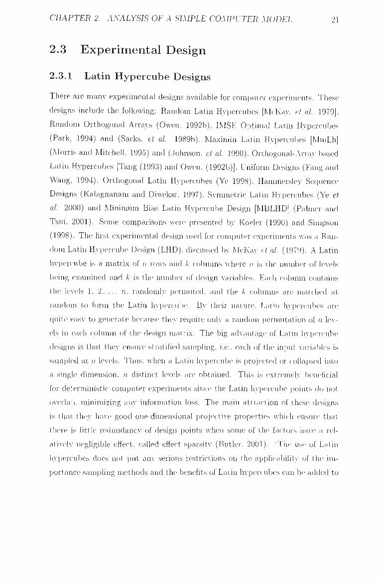
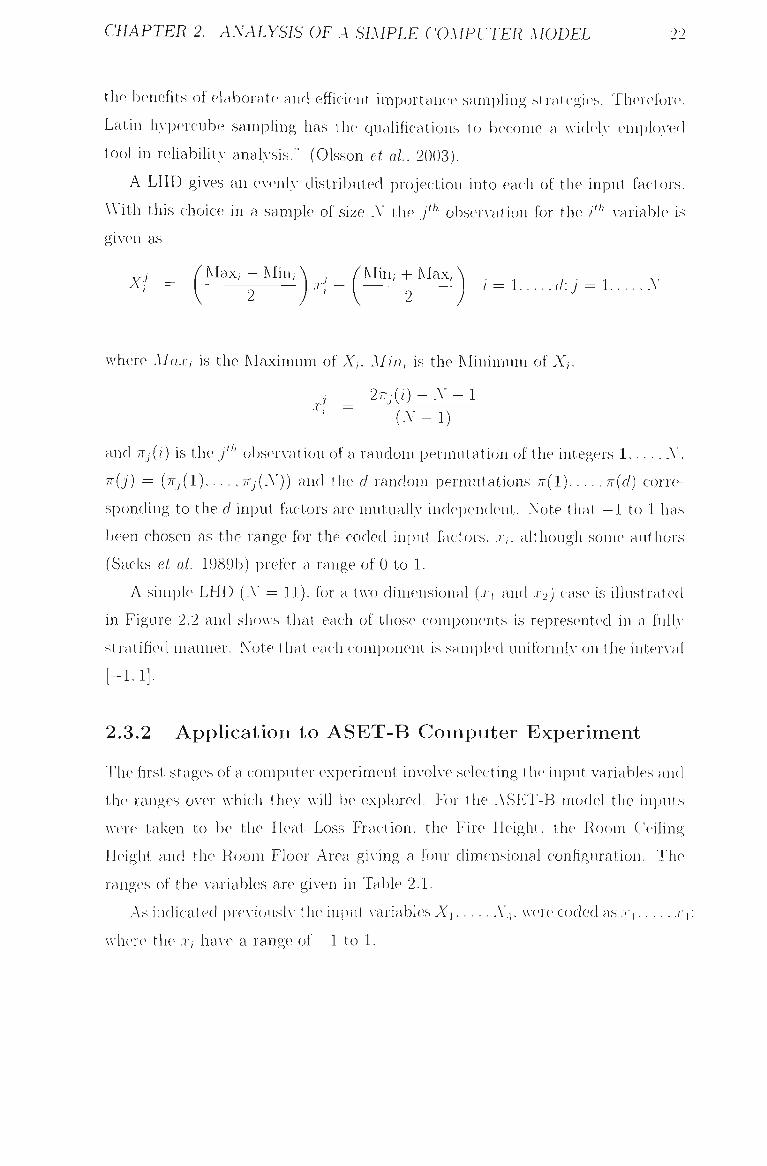
A simple LHD (W = 11), for a two dimensional (.r| and X2) case is illustrated
in Figure 2.2 and shoAvs that each of those components is represented in a full\-
stratified manner. Note tiiat each component is sampled uniformly on the inter\-al
[-1^1]-
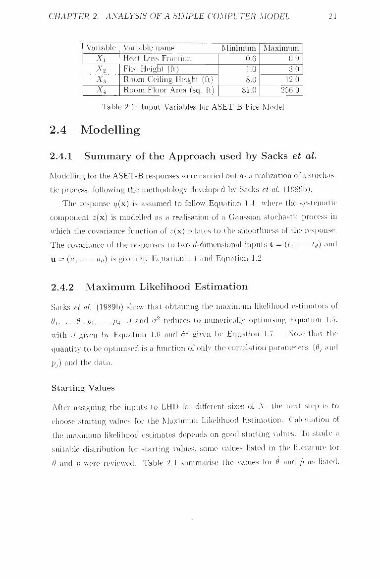
2.3.2 Application to ASET-B Compute r Exper iment
The first stages of a computer experiment involve selecting the input variables and
the ranges OAer Avhich they Avill be explored. For the ASET-B model the inputs
were taken to be the Heat Loss Fraction, the Fire Height, the Room Ceihng
Height and the Room Floor Area giAing a four dimensional configuration. The
ranges of the \^ariables are giA en in Table 2.1.
As indic-ated preA-iousl\' the input A'-ariables Xi,.. .. A'4, were coded as X[ r_i:
wlicn'c the .T, have a range of —1 to 1.
CHAPTER 2. ANALYSIS OF A SIMPLE COMPUTER MODEL 23
1.0
0.8
0.6
0.4
0.2
! 0.0
-0.2
-0.4
-0.6
-0.8
-1.0
-1.0 -0.8 -0.6 -0.4 -0.2 0.0 0.2 0.4 0.6 0.8 1.0 - 1 I ! ! ! I I I I i L _
n i i 1 1 \ 1— -1.0 -0.8 -0.6 -0.4 -0.2 0.0 0.2
xi
0.4 0.6 0.8
- 1.0
- 0.8
- 0.6
0.4
0.2
0.0
' -0.2
- -0.4
- -0.6
~ -0.8
-1.0
1.0
Figure 2.2: Projection Properties of a LHD with 11 runs.
The number of runs required remains an open ciuestion for computer exper
iments. Welch et al' (1996) suggest, as a guidefine. that the- number of runs in
a computer experiment should be chosen to be 10 timers the number of actiAc
inputs, Avhich would lead to A' = 40 runs for this example if all four factors turn
out to be actiA-e. To be conservatiA-e Y = 50 runs Avas used. More on sample size
considerations will be discussed in Chapter 3.
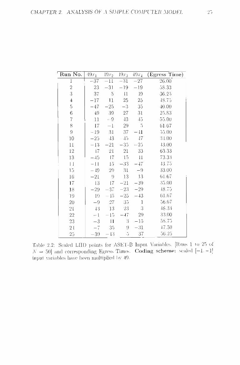
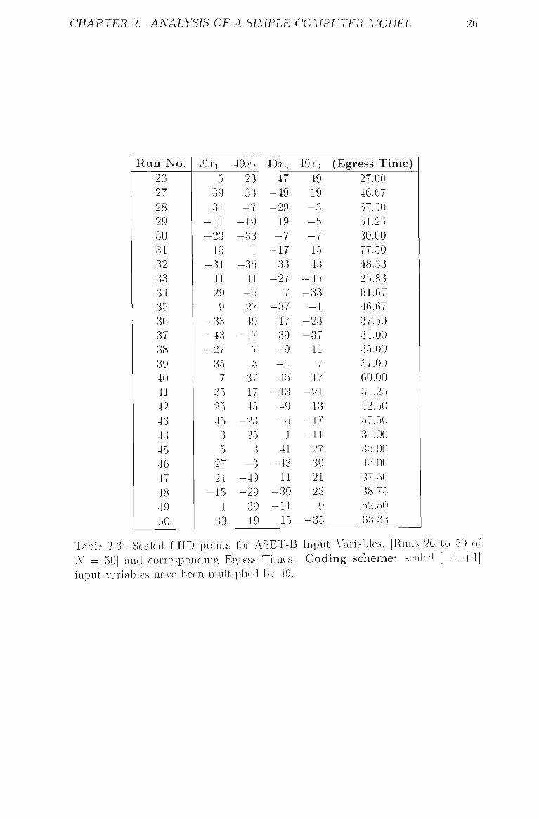
The actual input A-ariables and response (Egress Time), generated from the
ASET-B program, are given in Table 2.2, Table 2.3 and a pictorial reprc\sentatioii
of the design is giA en in Figure 2.3. The egress time for each run of the LHD Avas
calculated using linear interpolation bv assuming that the height of the smoke
layer is 5ft (head height).
CHAPTER 2. ANALYSIS OF A SIMPLE COMPUTER MODEL 24
Variable X,
X2 X, X,
Variable name Heat Loss Fraction Fire Height (ft) Room Ceiling Height (ft) Room Floor Area (sq. ft)
Minimum 0.6 1.0 8.0
81.0
Maximum 0.9 3.0
12.0 256.0
Table 2.1: Input Variables for ASET-B Fire Model
2.4 Modell ing
2.4.1 Summary of t he Approach used by Sacks et aL
Modelling for the ASET-B responses were carried out as a realization of a stochas
tic process, following the methodology dcA^eloped by Sacks et al. (1989b).
The response y(x) is assumed to folloAv Equation 1.4 Avhere the sA-stematic
component z(x) is modefled as a realisation of a Gaussian stochastic process in
Avhich the covariance function of -:(x) relates to the smoothness of the r(\s])onse.
The covariance of the responses to two d-dimensional inputs t = [ti.... .t^) and
u = ((/i,. . . ,Ud) is giA-en by Ecjuation 1.1 and Eciuation 1.2
2.4.2 Max imum Likehhood Est imat ion
Sacks et al. (1989b) shoAv that obtaining the maximum hkefihood estimators of
9i 94.P1, • • • -P^- ' and cr reduces to numerically optimising Eciuation 1.5,
Avith j] giA-en Ijy Equation 1.6 and (7 given by Equation 1.7. Note that the
ciuantity to be optimised is a function of only the correlation parameters, {9j and
Pj) and the data.
Starting Values
After assigning the inputs to LHD for different sizes of A', the next step is to
choose starting A-alues for the Maximum Likehhood Estimation. Calculation of
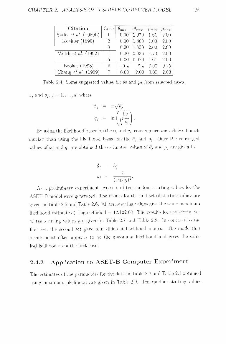
the maximum likelihood estimates depends on good starting values. To studA- a
suitable distribution for starting values, some A-alues listed in the literature for
9 and p were revicAved. Table 2.4 summarise the A-alues for 9 and p as listed.
CHAPTER 2. ANALYSIS OF A SIMPLE COMPUTER MODEL 25
Run No. 1 2 3 4 5 6 7 8 9 10 11 12 13 14 15 16 17 18 19 20 21 22 23 24 25
49xi
-37 23 37
-17 -47 49 11 17
-19 -25 -13 47
-45 -11 -49 -21 13
-29 19 -9 43 -1 -3 — 7
-39
49.r2
-11 -31
5 11
-25 39 -9 -1 31 43
-21 21
-47 15 29 9 47
-37 -45 -27 13
-15 -41 35
-43
49x3
-31 -19 -41 25 -3 27 43 29 37
-45 -35 21
-15 -33 31 13
-21 -23 -25 35 23
-47 3 9 5
49.X4
-27 -19 -49 25 35 31 45 5
-41 47
-25 33 41
-47 -9 13
-39 -29 -43
1 3 29
-15 -31 37
(Egress Time)
26.00
58.33
36.25
48.75
40.00
25.83
55.00
61.67
55.00
34.00
43.00
63.33
73.33
43.75
33.00
61.67
35.00
48.75
61.67
56.67
48.33
33.00
58.75
47.50
56.25
Table 2.2: Scaled LHD points for ASET-B Input Variables. [Runs 1 to 25 of iV = 50] and corresponding Egress Times. Coding scheme: scaled [-L+1] input A-ariables haA e been multiplied l)>- 49.
CHAPTER 2. ANALYSIS OF A SIMPLE COMPUTER MODEL 26
Run No. 26 27 28 29 30 31 32 33 34 35 36 37 38 39 40 41 42 43 44 45 46 47 48 49 50
49.ri
5 39 31
-41 -23 15
-31 41 29 9
-33 -43 -27 -35
7 35 25 45 3
-5 27 21
-15 1 33
49:r,
23 33 —7 -19 -33
1 -35 41 —5 27 49
-17 7
-13 37 17 45
-23 25 3
-3 -49 -29 -39 19
49x3
47 -49 -29 19 -7 -17 33
-27 7
-37 17 39 -9 -1 45
-13 49 —5 1 41
-43 11
-39 -11 15
49.r4
49 19 -3 -5 -7 15 43
-45 -33 -1 -23 -37 11 7 17
-21 -13 -17 -11 27 39 21 23 9
-35
(Egress T i m e )
27.00
46.67
57.50
51.25
30.00
77.50
48.33
25.83
61.67
46.67
37.50
34.00
35.00
37.00
60.00
31.25
42.50
57.50
37.00
35.00
45.00
37.50
38.75
52.50
63.33
Table 2.3: Scaled LHD points for ASET-B Input \ariables, [Runs 26 to 50 of Y = 50] and corresponding Egress Times. Coding scheme: scaled [-1,+1] input A-ariables haA-e been multiplied bA- 49.

CHAPTER 2. ANALYSIS OF A SIMPLE COMPUTER MODEL 27
X1
• . • • . _
•^.0 -0,5 0.0 0,5 1,0
• , * ' ,
X2
• . '
• . * • • . • .
1,0 -0 5 0,0 0 5 1,0
• ' • •
' . , • •
'. • \ •
. • . • • • . '
. " • •
• • .
X3
• ' . •
. • .
X4
-1,0 -0,5 0,0 0,5 1,0 -1,0 -0,5 0,0 0,5 1,0
Figru'e 2.3: Projection Properties of a LHD with 50 runs.
According to the indicated magnitudes of ^'s and p's: the ^s lie between 0 and 2
and the ps will also be bet\\-een 0 and 2.
Based on this evidence, the method adopted Avas to generate^ 10 random sets of
starting A-alues and for each set to calculate the maximum likelihood estimates.
The random starts for the parameters Pj, j = 1,... ,d, were generated from a
uniform distribution on [0,2], AA-hile the random starts for the 9j. j = 1, d.
w-ere generated from an exponential distribution Avith mean 1. Of course other
distributions could be used.
Calculating the maximum likelihood estimates is a constrained optimisation
problem since 0 < Pj < 2, j = 1.. .d and 0 < 9j j = 1.. .d.
More success resulted b\- turning the constrained optimisation problem im-oh--
ing 9i ,9d,Pi, • • • ,Pd into an unconstrained optimisation involving parameters
CHAPTER 2. ANALYSIS OF A SIMPLE COMPUTER MODEL 28
Citation Sacks et al (1989b)
Koehler (1990)
Welch et al (1992)
Booker (1998) Chang et al (1999)
Case 1 2 3 4 5 6 7
"min
0.00 0.00 0.00 0.00 0.00 -0.4 0.00
"max
1.970 1.800 1.850 0.036 0.970
0.4 2.00
Pmin Pmn.T
1.61 2.00 1.00 2.00 2.00 2.00 1.70 2.00 1.61 2.00 0.00 0.25 0.00 2.00
Table 2.4: Some suggested values for ^s and ps from selected cases.
rpj and qj, j = 1,... ,d, where
© 7
Qj
By using the likelihood based on the Oj and cjj, com-ergence Avas achieved much
quicker than using the likefihood based on the 9j and j)j. Once the com-erged
values of (j)j and qj are obtained the estimated \-alues of 9j and Pj are giA-en b\-
o -, 2
^^ (expgj)2'
As a preliminarA- experiment tAvo sets of ten random starting values for the
ASET-B model AV( re generated. The results for the first set of starting \-alues are
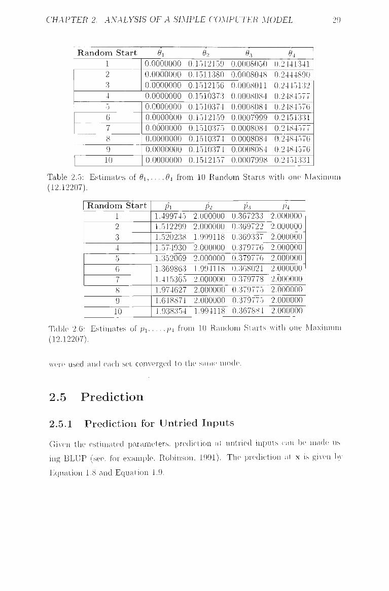
given in Table 2.5 and Table 2.6. AU ten starting A-alues give the same maximum
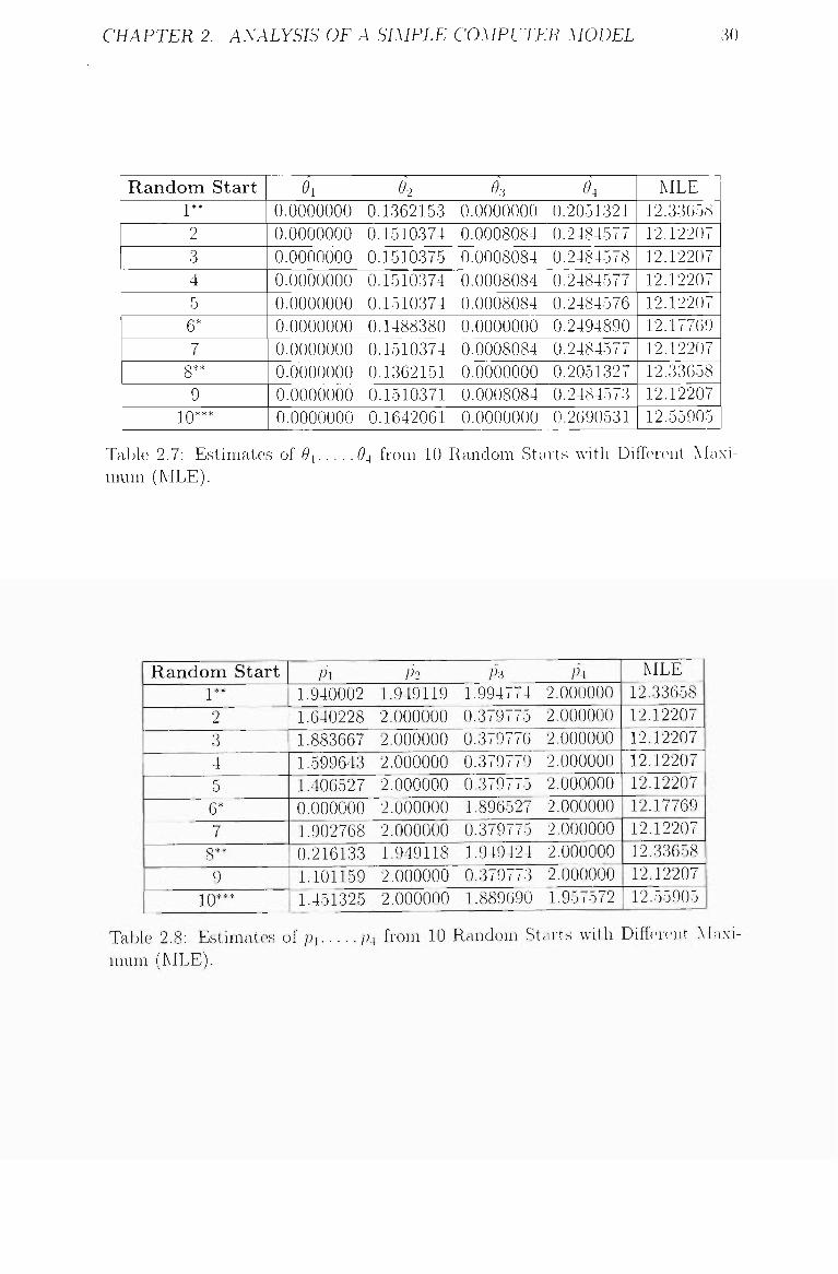
likelihood estimates (-loghkelihood = 12.12207). The resufis for the second set
of ten starting values are giA-en in Table 2.7 and Table 2.8. In contrast to th(
first set, the second set gave four different likelihood modes. The mode that
occurs most often appears to be the maximum likelihood and giA-es the same
loghkelihood as in the first case.
2.4.3 Apphcation to ASET-B Computer Experiment
The estimates of the parameters for the data in Table 2.2 and Table 2.3 ol)tained
using maximum hkelihood are giA-en in Table 2.9. Ten random starting A-alues
CHAPTER 2. ANALYSIS OF A SIMPLE COMPUTER MODEL 29
Random Start 1 2 3 4 5 6 7 8 9 10
9i 02 9-, 6*4
0.0000000 0.1512159 0.0008050 0.2441341
0.0000000 0.1511380 0.0008048 0.2444890
0.0000000 0.1512156 0.0008011 0.2445132
0.0000000 0.1510373 0.0008084 0.2484577
0.0000000 0.1510374 0.0008084 0.2484576
0.0000000 0.1512159 0.0007999 0.2451331
0.0000000 0.1510375 0.0008084 0.2484577
0.0000000 0.1510374 0.0008084 0.2484576
0.0000000 0.1510374 0.0008084 0.2484576
0.0000000 0.1512157 0.0007998 0.2451331
Table 2.5: Estimates of 6*1,... ,^4 from 10 Random Starts Avith one Maximum
(12.12207).
Random Start 1 2 3 4 5 6 7 8 9 10
P'l p'2 Ps ih 1.499745 2.000000 0.367233 2.000000
1.512299 2.000000 0.369722 2.000000
1.520238 1.999118 0.369337 2.000000
1.574930 2.000000 0.379776 2.000000
1.352069 2.000000 0.379776 2.000000
1.369863 1.994118 0.368021 2.000000
1.415365 2.000000 0.379778 2.000000
1,974627 2.000000 0.379775 2.000000
1.618871 2.000000 0.379775 2.000000
1.938354 1.994118 0.367884 2.000000
Table 2.6: Estimates of p i , . . . , p 4 from 10 Random Starts Avith one Maximum
(12.12207).
\A-ere used and each set converged to the saiii(> mode.
2.5 Prediction
2.5.1 Prediction for Untried Inputs
GiA-en the estimated parameters, prediction at untried inputs can be made us
ing BLUP (see, for example, Robinson, 1991). The prediction at x is giA-en IJA-
Equation 1.8 and Equation 1.9.
CHAPTER 2. ANALYSIS OF A SIMPLE COMPUTER MODEL 30
Random Start 1 **
2 3 4 5 6* 7 8** 9
-1 rv * * *
01
0.0000000
0.0000000
0.0000000
0.0000000
0.0000000
0.0000000
0.0000000
0.0000000
0.0000000
0.0000000
02
0.1362153
0.1510374
0.1510375
0.1510374
0.1510374
0.1488380
0.1510374
0.1362151
0.1510371
0.1642061
03 0.0000000
0.0008084
0.0008084
0.0008084
0.0008084
0.0000000
0.0008084
0.0000000
0.0008084
0.0000000
04 0.2051321
0.2484577
0.2484578
0.2484577
0.2484576
0.2494890
0.2484577
0.2051327
0.2484573
0.2690531
MLE 12.33058
12.12207
12.12207
12.12207
12.12207
12.17769
12.12207
12,33658
12.12207
12.55905
Table 2.7: Estimates of 6*1 04 from 10 Random Starts Avith Different Maximum (MLE).
Random Start 1 **
2 3 4 5 6* 7 8** 9
1 n***
Pi 1,940002
1.640228
1.883667
1.599643
1.406527
0.000000
1.902768
0.216133
1.101159
1.451325
P2 1.949119
2.000000
2.000000
2.000000
2.000000
2.000000
2.000000
1.949118
2.000000
2.000000
Ps 1.994774
0.379775
0.379770
0.379779
0.379775
1.896527
0.379775
1.949424
0.379773
1.889690
P4 2.000000
2.000000
2.000000
2.000000
2.000000
2.000000
2.000000
2.000000
2.000000
1.957572
MLE 12.33658
12.12207
12.12207
12.12207
12.12207
12.17769
12.12207
12.33658
12.12207
12.55905
Table 2.8: Estimates of pi p^ from 10 Random Starts Avith Diffc-rcnit Maximum (MLE).

CHAPTER 2. ANALYSIS OF A SIMPLE COMPUTER MODEL 31
J Oj
PJ
ft C72
1 0.00934 1.98051 48.3526 123.556
2 0.02041 1.89041
3 0.01953 1.99708
4 0.02849 2.00000
Table 2.9: Estimates of Parameters for the ASET-B Computer Model.
2.5.2 Prediction Error
For a prediction to be useful it should be supplemented In- a measure of its
precision. A number of different measures haA-e been introduced for computer
experiments. Their utility has been reviewed bA- Sacks et al. (1989a). The most
important measures are:
Empirical Mean Square Error
EMSE=|lX]l^W-yW]4 (-'•!)
Avhere x is a set of N raiidoiiil\- selected points over the experimental region TZ.
A related measure is
Empirical Root Mean Square Error
ERMSE = i^5][y(x)-y(x) A'
f2.2)
Mean Square Error at a point x
MSE[y(x)] = a' 1 - 1 r^(x) 0 V
1 R D
Maximum Mean Square Error
Max,e7Z^ISE(.y(x))
1
r(x) (2.3)
2.4^
Integrated Mean Square Error
MSE(y(x)). •Jy.eTl
, ^ .0
CHAPTER 2. ANALYSIS OF A SIMPLE COMPUTER MODEL 32
2.5.3 Apphcation to ASET-B Computer Experiment
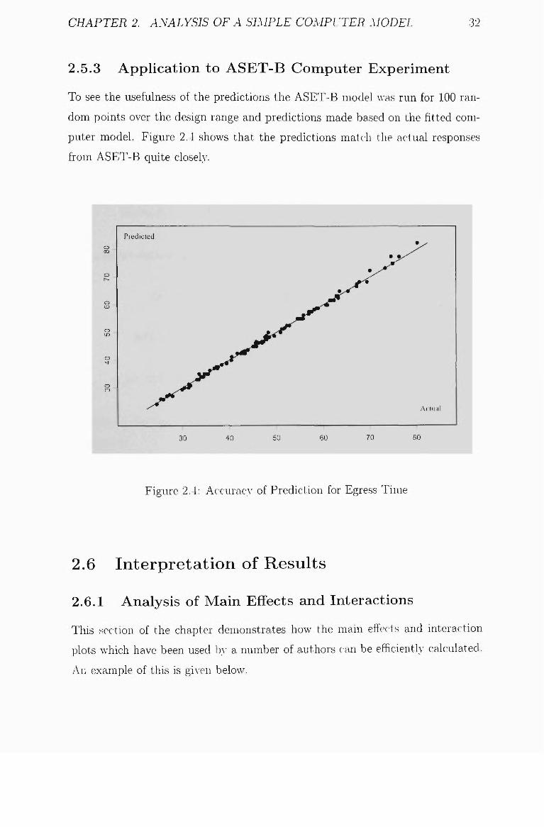
To see the usefulness of the predictions the ASET-B model was run for 100 ran
dom points over the design range and predictions made based on the fitted com
puter model. Figure 2.4 shows that the predictions match the actual responses
from ASET-B quite closely.
Figure 2.4: AccuracA- of Prediction for Egress Time
2.6 Interpretation of Results
2.6.1 Analysis of Main Effects and Interactions
This section of the chapter demonstrates how the main effects and interaction
plots Avhich have been used 1)A- a number of authors can be efficiently calculated.
.All example of this is giA-en below.
CHAPTER 2. ANALYSIS OF A SIMPLE COMPUTER MODEL 33
Sacks et al. (1992) defined, for a computer model Avith input range u € [0.1]* .
the mean, main effects and interaction effects as
Po = / ••• / .?/(u)]^c/u/,
[0,1]' ' '""'
/ii(a,) = ••• y{u)Ylduh- tiQ
l.i,,j{u,,Uj) = •• y{u) Yl '^"'> ~ / ' ' (" ' ) ~ ^j("j) ^ - 0-[0,1]^ ^^^J
For a model defined on z G [—1,1]' the definitions become
Mo = T / - • • / .?/(z) n ^ ^ 2d - l . l ] " ' ^ = 1
• [ - L l ] " ''^'•^
In practice, the true effects are estimated b}- replacing y{z) hy y{z) in the alxn-e
expressions.
Since the BLUP estimator of y is giA-c n IJA- Eciuation 1.8 then the estimator y
can be re-written as:
•y(z) = ;'i + r'^(z)w
AA-liere
w^Kf^ij-lft)
and r(z) is giA-en bA- Eciuation 1.9. Hence y(z) can be CA-aluated as
y{z) = fj + a'ii?(Xi. Z) + U'27?(X2, Z) + . . . + U'„7?(x„. Z)
for an arbitrarA- input point z.
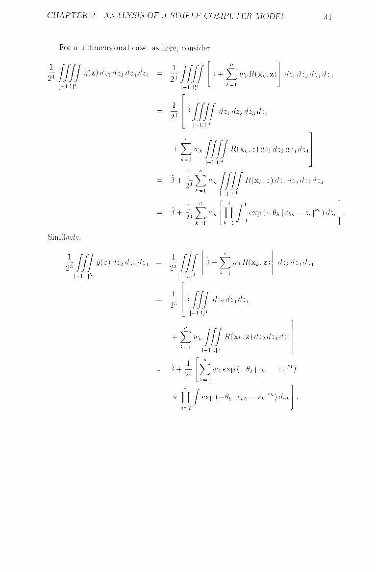
CHAPTER 2. ANALYSIS OF A SIMPLE COMPUTER MODEL 34
For a 4 dimensional case, as here, consider
1 y(z) dzi dz2 dz'i dz^
- i . i l
1
¥
1
2^
-1.11
.? +J^u; , i? (xfc ,z) fc=i
dz\ dzo d::i dzji
^ 1 1 dzj dz2 dz-i dz4
-1.1]^
+ X ^ ll-'k / / / / ^ (Xfc , z) f/2i dz2 dZ:i dz4
^^'^ [-1.1H
^ + ^ E ' 'W / / / ( ' ^ ') '^'^ ~2 '/ i 'h^ k=l
-hiV
'^+Y^fl'''^- n / exp(-9,\x,,,-z,r)dz, k=i h = \
Similarlv.
,3 / / / y(^) d--^ ^--i d-^
-1,11^
1
I
1
9^
-1,113
• H ^ » > / ? ( X 4 . . Z ) A = l
f/.:2 d.2:i <I^4
3 dz, dz. dz 3 " - 4
-1.1
A = l
+ 5 ^ (('A. / / / ^(XA-. Z) r/ 2 c/-3 dZ4
l-l.lp
^ ((•/,. exp (-6*1 [.Cfci - ^l|^' H fc=i
h=2 -^
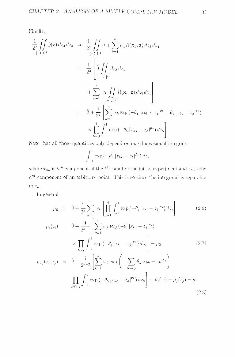
CHAPTER 2. ANALYSIS OF A SIMPLE COMPUTER MODEL 35
Finalh-,
22 J J ^^^"^ "^^^ "^^^ " 22 1-1.ip 1
1
ft + ^ li'kRi^k- z) dz:i dz4
-1,1]2 k=l
3 I I dzs dz4
I-i,'iP
+ ^ ^'k / / -R(xfc, z) dzs dz4 k=\
= ^ + Y^
[ -1 ,1P
n
X
^ Wk exp ( -^1 |,Tfci - zil"' - 02 [r^.2 k=l
n / exp(- .^ , ] , r , , -2 , , |^")c/ - / i , _ o 7 - i
-, |P2^ - 2 ,
Note that all these quantities onl}- depend on one-dimensional integrals
/ exp(-^;, | . r hk — ^k\ ) <l^k
where x^]^ is h*'^ component of the A-* point of the initial experiment and z^ is the
j^th component of an arbitrarA' point. This is so since the integrand is separable
in Zh-
In general
d „ i
p,(z,,) = .3 +
k=l lj = l-^~^
n
y ^ »'fc exp (-^,- I.Tfcj - Zjl"') 2d-1
,fc=i
X n / ' e x p ( - ^ , | „ r , , - z , r ) c / : hyti--'-'^
A'o (2.7)
/' ( . j \ - ( - ^ , / , ^ + 2^-^ y ^ (/'A-exp - 5 ^ /il •X/t/i - ^ / i ^ ' ^
,fe=i h=i.j
J l / exp(-^^|.Tfch-2/i|^'0c?2ft 1.1,{Z,) - P j ( 2 j ) - / ^ o -
(2.8)
CHAPTER 2. ANALYSIS OF A SIMPLE COMPUTER MODEL 36
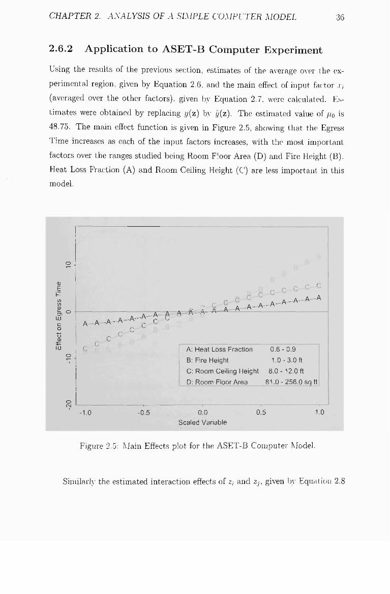
2.6.2 Apphcation to ASET-B Computer Experiment
Using the results of the previous .section, estimates of the aA-erage oA-er the ex
perimental region, given by Equation 2.6, and the main effect of input factor x,
(averaged over the other factors), given b}- Equation 2.7. were calculated. Es
timates were obtained by replacing y(z) bv jj{z). The estimated value of po is
48.75. The main effect function is given in Figure 2.5, showing that the Egress
Time increases as each of the input factors increases, with the most important
factors over the ranges studied being Room Floor Area (D) and Fire Height (B).
Heat Loss Fraction (A) and Room Ceiling Height (C) are less important in this
model.
0)
E
w <D i _ CD LU c o
"o
CD
LU
= 5 = ^
,, r.-C O^ p , - - u
r C- ^ . « a-—A—A—/^
Jl-A-A-_A^A---A'
o
A'
C
, A - A - A '
,C .X'-A:
B:
C
D:
Heat Loss Fraction
Fire Height
Room Ceiling Height
Room Floor Area
0.6
1.0
8.0-
81.0-
-0.9
-3,0 ft
12.0ft
256.0 sq ft
-1.0 -0.5 0.0 Scaled Variable
0.5 1.0
Figure 2.5: Main Effects plot for the ASET-B Computer Model.
Similarly the estimated interaction effects of z, and Zj, given bA' Equation 2.8
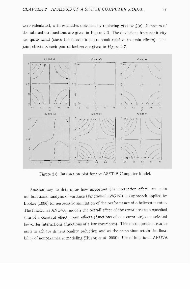
CHAPTER 2. ANALYSIS OF A SIMPLE COMPUTER MODEL 37
Avere calculated, Avith estimates obtained bv replacing y{z) by y{z). Contours of
the interaction functions are given in Figure 2.6. The deviations from additivity
are quite small (since the interactions are small relative to main effects). The
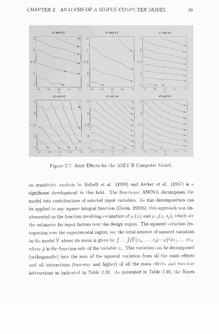
joint effects of each pair of factors are given in Figure 2.7.
x1 and x2
o\5 p -g 5
•1,0 -0,5 0 0 0,5
x2 and x3
-05 0,0
x1 and x3
-0 5
J
1 ^
3
r
-10 -0,5 0 0 0,5 1,0
x2 and x4
•/s / -V.s J -d5
a M \ ''J' ^ o>5
\ • 0
x1 and x4
^5 \ 0 5
^ ^ 5
•- 0
1 -0/5 / _,4
-0 5 0 0 05 to
x3 and x4
-^^^ -V5 J' -q5
S^sV l\5 \ Ols
\ \ \ 5
1 45 / .y{ ^
Figure 2.6: Interaction plot for the ASET-B Computer Model.
Another AvaA' to determine hoAv important the interaction effects are is to
use functional analysis of variance {functional ANOVA), an approach applied bA-
Booker (1996) for aeroelastic simulation of the performance of a helicopter rotor.
The functional ANOVA, models the overall effect of the covariates as a specified
sum of a constant effect, main effects (functions of one covariate) and selected
low-order interactions (functions of a feAv covariates). This decomposition can be
used to achieve dimensionality reduction and at the same time retain the flexi
bility of nonparametric modefing (Huang et al 2000). Use of functional ANOVA
CHAPTER 2. ANALYSIS OF A SIMPLE COMPUTER MODEL 38
x2
-1,0
-0
.5
0,0
05
10
x3
1,0
-0,5
0,
0 0,
5 1,
0
Ei
x1 and x2
-~,.^^^ 66
-1,0 -05 0 0 0 5 1-0 xi
x2 and x3
o | : -1.0 -0.5 0.0 0,5 1.0
x2
X c
x4
10
-0 5
0
0 0.
5 1.
0
x1 and x3
- - ; : :
-1.0 -0.5 0.0 0.5 1.0 xi
x2 and x4
\ X \ \ \ ®
-1,0 -0 5 0.0 0.5 1 0
x2
c
o
q
q
O
O
x1 and x4
Pl -—~I ~~—-—-« — - ^ ^
-1.0 -0 5 0 0 0 5 1-0 xi
x3 and x4
:ii -1,0 -0 5 0 0 0,5 1 0
x3
Figure 2.7: Joint Effects for the ASET-B Computer Model.
on sensitiA'ity analA-sis by SalteUi et al. (1999) and Archer et al. (1997) is a
significant development in this field. The functional ANOVA decomposes the
model into contributions of selected input variables. As this decomposition can
be applied to any square integral function (OAA en. 1992b). this approach Avas im
plemented to the function invohung (estimation of//,(2,) and p,.j{z,. Zj), which are
the estimates for input factors OAer the design region. The squared variation (in
tegration OA-er the experimental region: say the total amount of squared A^ariation
in the model Y about its mean is giA-en bv / • •. / (V( . r i , . . . , .r^) - p)^dxi ... dx,i.
AA-here p is thc function only of the A-ariable x,. This variation can be decomposed
(orthogonalh-) into the sum of the squared A-ariation from all the main effects
and all interactions (tAvo-AvaA- and higher) of all the main efiects and tAvo-AA-aA-
interactions as indicated in Table 2.10. As presented in Table 2.10, the Room
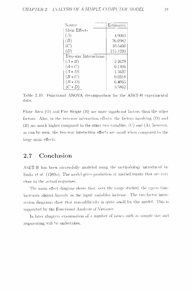
CHAPTER 2. ANALYSIS OF A SIMPLE COMPUTER MODEL 39
Source Main Effects (A) (B) (C) (D) Two-way Interactions {A*B) {A*C) (yl*L>) ( 5 * C ) {B*D) {C*D)
Estimates
4.9003 76.6982 30.5498
215.1293
2.2679 0.1406 1.5637 0.0318 6.4065 3.5862
Table 2.10: Functional ANOVA decomposition for the ASET-B experimental data.
Floor Area (D) and Fire Height (B) are more significant factors than the other
factors. Also, in the tAvo-\A'ay interaction effects, the factors involving (D) and
(B) are much higher compared to the other tAvo A-ariables, (C) and (A), hoAvever.
as can be seen, the tAvo-AvaA' interaction effects are small Avheii compared to the
large main effects.
2.7 Conclusion
ASET-B has been successfully modeled using the methodology introduced bA'
Sacks et al. (1989a). The model giA-es prediction at untried inputs that are ver>-
close to the actual responses.
The main effect diagram shoAVS that, OAer the range studied, the egress time
increases almost linearly as the input variables increase. The tAvo-factor inter
action diagrams shoAv that uon-additiA-itA- is quite small for this model. This is
supported by the Functional Analysis of Variance.
In latc-r chapters examination of a number of issues such as sample size and
augmenting Avill be undertaken.
Chapter 3
Sample Size Considerations
3.1 Introduction and Background
One of the open problems in computer experiments is hoAv mam- runs a computer
experiment should haA-e. In attempting to ansAA-er this question Welch et al.
(1992), suggested [.. .] •' taking 10 times the number of active inputs (admittedly
a guess)". Indeed a method of adding a number of runs to a computer experiment
or deciding on a sample size for a computer experiment prior to the experiment
AA ould Ije highly useful for scientists working Avith computer experiments.
K()(4iler (1990) performed a study on the behaA'iour of maximum likelihood
estimators (of ft. a^ and 0) when the sample size is changed. In his studA- the de
sign space was fixed for different correlation families. He suggested that relatiA-eh'
small sample sizes for computer experiments in terms of maximum likelihood es
timators may A-ield poor results. Further, the study highlighted the side effect of
too maiiA- samples in Avhich an increase in the sample size Avill not improve the
maximum likelihood estimators. He proposed a rule for the maximum sample
size as n,nax = 10 * c/, (Avhere d is dimension of input A-ariables of the computer
code selected) only for efficiency of estimation and not necessarih- for good oA'crall
prediction.
This chapter Avill address the issue of sample size for good prediction ])y exper
imenting on four selected computer models. These models are ASET-B (details
40
CHAPTER .3. SAMPLE SIZE CONSIDERATIONS 41
are in Chapter 2), Detector Actuation Quasi Steady [DETACT-QS] (EA-ans and
Stroup 1985), Circuit Simulation model using the design of a W'heatstone Bridge
[CIRC] (Box and Fung 1986) and Detector Actuation Time Squared [DETACT-
T2] (Evans and Stroup 1985) respectiveh'. The details of these computer models
will be discussed in the next section.
3.2 Some Details of the Selected Computer
Models
3.2.1 DETACT-QS
This computer model Avhich determines the response of fixed temperature and rate
of rise heat detectors to fire Avith energA- release rates described bA' the expression
Q — at^. The complex equations are solved using NeAvton-Raphson techniques.
DETACT-QS can be used to predict the actuation time of fixed temperature
heat detectors and sprinkler heads subject to a user specified fire. DETACT-QS
assumes that the thermal device is located in a relatiA-ely large arcvi. that only the
fire ceiling floAv heats the dcA-ice, and there is no heating from the accumulated
hot gases in the room. The required model inputs are the height of the ceiling
aboA e the fire, the distance of the detector from the axis (DDA). the actuation
temperature of the thermal device (DAT), the response time index (RTI) for the
device, and the rate of heat release of the fire. The required range of inputs are
fisted in Table 3.1, The computer model outputs are the ceiling gas temperature
and the device temperature both as a function of time and the time reciuired for
device actuation.
DETACT-QS Avas used as the second four dimensional case A\-ith a medium
fire growth rate being specified. The computer code output recorded and analysed
was the time required for device actuation.
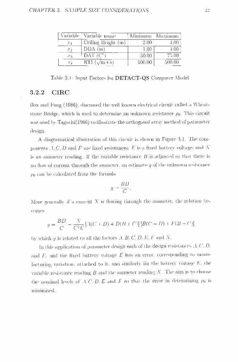
CHAPTER 3. SAMPLE SIZE CONSIDERATIONS 42
Variable .Xi
•^2
^S
X4
Variable name Ceiling Height (m) DDA (m) DAT (C") RTI (Vm * s)
Minimum 2.00 1.00
50.00 100.00
Maximum 4.00 4.00
75.00 500.00
Table 3,1: Input Factors for DETACT-QS Computer Model
3.2.2 CIRC
Box and Fung (1986), discussed the w ell know-n electrical circuit caUed a Wlreat-
stone Bridge, which is used to determine an unknown resistance po- This circuit
was used by Taguchi(1986) to illustrate the orthogonal array method of parameter
design.
A diagramatical illustration of this circuit is shoAvn in Figure 3.1. The com
ponents ,1. C, D and F are fixed resistances; E is a fixed batter>- A-oltage: and N
is an ammeter reading. If the A-ariable resistance B is adjusted so that there is
no flow of current through the ammeter, an estimate y of the unknoAA-n r(>sistance
po can be calculated from the formula
BD y c
More generallA- if a current A' is floAving through the ammeter, the relation be
comes
BD N [A{C -f D) + D{B + C)] [B{C + D) + F{B + C)]
" C C^E
b.A- Avhich y is related to ah the factors .1. B, C, D, E, F and A'.
In this apphcation of parameter design each of the design resistances .1. C. D.
and F. and the fixed battery A-oltage E has an error, corresponding to manu
facturing \-ariation. attached to it, and similarly for the batterv A-oltage E. the
variable resistance reading B and the ammeter reading X. The aim is to choose
the nominal IcA-els oi A.C.D,E and F so that the error in determining po is
minimised.
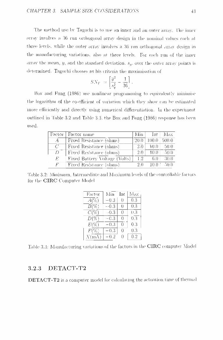
CHAPTER 3. SAMPLE SIZE CONSIDERATIONS 43
The method use !)>- Taguchi is to use an inner and an outer arraA-. Tlie inner
arraA- im-oh-es a 36 run orthogonal array design in the nominal values each at
three ICA'CIS. Avhile the outer array involves a 36 run orthogonal arraA- design in
the manufacturing variations, also at three levels. For each run of the inner
arraA' the mean, y, and the standard deviation, Sy. OAer the outer arraA' points is
determined, Taguchi chooses as his criteria the maximisation of
SX T t 1 ^l 36
Box and Fung (1986) use nonlinear programming to equiA-alent 1A' minimise
the logarithm of the co-efficient of variation Avhich thcA' show can be estimated
more efficiently and directly using numerical differentiation. In the experiment
outlined in Table 3.2 and Table 3.3. the Box and Fung (1986) response has been
used.
Factor A C D E F
Factor name Fixed Resistance (ohms) Fixed Resistance (ohms) Fixed Resistance (ohms) Fixed Battery Voltage (Volts) Fixed Resistance (ohms)
Min 20.0
2.0 2.0 1.2 2.0
Int 100.0
10.0 10.0 6.0
10.0
Max 500.0
50.0 50.0 30.0 50.0
Table 3.2: IMinimum, Intermediate and Maximum leA els of the controllable factors for the CIRC Computer Model
Factor A{%) B{%)
C{%) D{%)
E{%) F{%)
A'(mA)
Min -0 .3 -0 .3 - 0 . 3 - 0 . 3 - 0 . 3 - 0 . 3 -0 .2
Int 0 0 0 0 0 0 0
Max 0.3 0.3 0.3 0.3 0.3 0.3 0.2
Table 3.3: Manufacturing A'ariations of the factors in the CIRC computer Model
3.2.3 DETACT-T2
DETACT-T2 is a computer model for calculating the actuation time of thermal
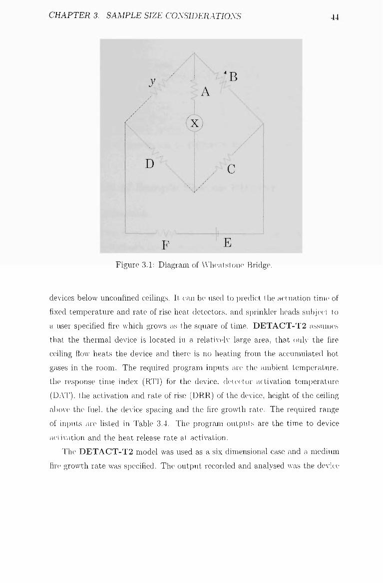
CHAPTER 3. SAMPLE SIZE CONSIDERATIONS 44
Figure 3.1: Diagram of W'heatstone Bridge.
devices below unconfined ceilings. It can be used to predict the actuation time of
fixed temperature and rate of rise heat detectors, and sprinkler heads subject to
a user specified fire which groAA's as the scjuare of time. DETACT-T2 assumes
that the thermal device is located in a relatiA-ely large area, that onh- the fire
ceiling flow heats the device and there is no heating from the accumulated hot
gases in the room. The required program inputs are the ambient temperature,
the response time index (RTI) for the device, detector activation temperature
(DAT), the activation and rate of rise (DRR) of the device, height of the ceifing
aboA'e the fuel, the clcA-ice spacing and the fire groAvth rate. The required range
of inputs are hsted in Table 3.4. The program outputs are the time to deAdce
ac-li\'ation and the heat release rate at actiA^ation.
The DETACT-T2 model Avas used as a six dimensional case and a medium
fire groAvth rate Avas specified. The output recorded and analysed Avas the dcA-ice
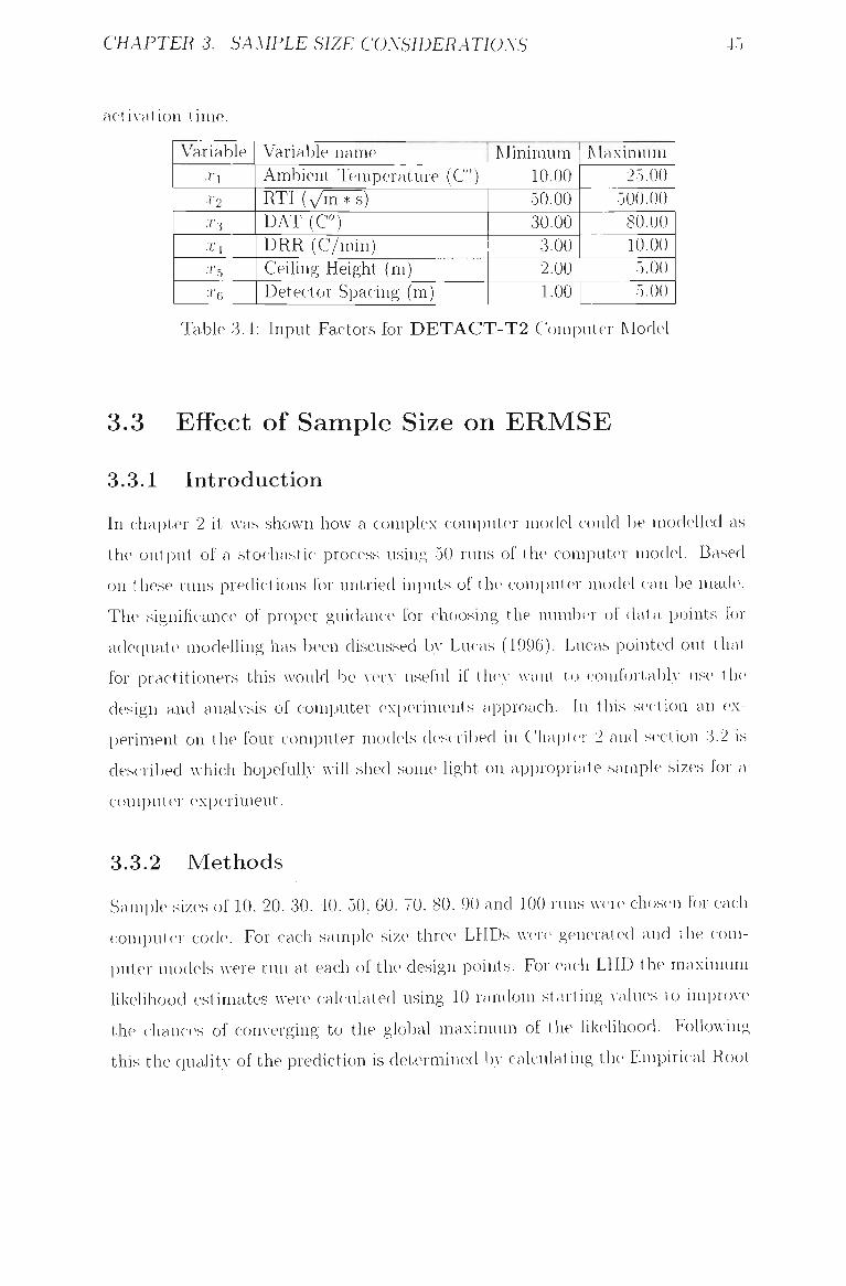
CHAPTER 3. SAMPLE SIZE CONSIDERATIONS
actiA-ation time.
Variable Xi
•^2
•-^•3
X4
•T.5
•Te
Variable name Ambient Temperature (C°) RTI (Vm * s) DAT (C°) DRR (C/min) Ceiling Height (m) Detector Spacing (m)
Minimum 10.00 50.00 30.00 3.00 2.00 1.00
Maximum 25.00
500.00 80.00 10.00 5.00 5.00
Table 3.4: Input Factors for DETACT-T2 Computer Model
3.3 Effect of Sample Size on E R M S E
3.3.1 Introduction
In chapter 2 it Avas shown hoAv a complex computer model could be modelled as
the output of a stochastic process using 50 runs of the computer model. Based
on these runs predictions for untried inputs of the computer model can be made.
The significance of proper guidance for choosing the nvmrber of dal a points for
adequate modelhng has been discussed In- Lucas (1996). Lucas pointed out that
for practitioners this Avould be A-erA' useful if the>' A\'ant to comfortabh- use the
design and anah-sis of computer experiments approach. In this section an ex
periment on the four computer modc4s described in Chapter 2 and section 3.2 is
described Avhich hopefulh- Avill shed some light on appropriate sample sizes for a
C( )input er experiment.
3.3.2 Methods
Sample sizes of 10, 20, 30, 40. 50, 60. 70, 80, 90 and 100 runs Avere chosen for each
computer code. For each sample size three LHDs Avere generated and the com
puter models Avere run at each of the design points. For each LHD the maximum
likelihood estimates Avere calculated using 10 random starting values to improA-e
the chances of con\-erging to the global maximum of the likelihood. FolloAving
this the qualitA- of the prediction is determined I A- calculating the Empirical Root
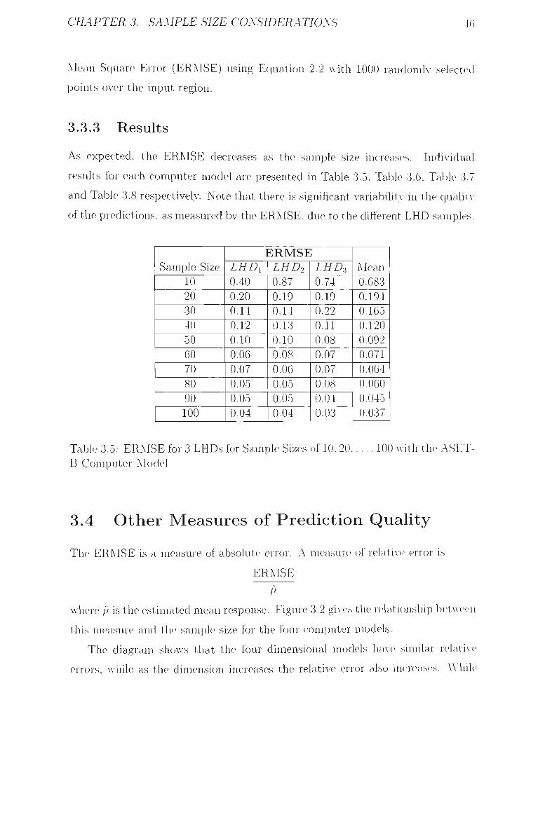
CHAPTER 3. SAMPLE SIZE CONSIDERATIONS 40
Mean Square Error (ERMSE) using Equation 2.2 Avith 1000 randomlv selected
points over the input region.
3.3.3 Results
As expected, the ERMSE decreases as the sample size increases. Individual
results for each computer model are presented in Table 3.5, Table 3.6, Table 3.7
and Table 3.8 respectively. Note that there is significant A ariabifitA- in the qualitA-
of the predictions, as measured by the ERIMSE, due to the different LHD samples.
Sample Size 10 20 30 40 50 60 70 80 90 100
E R M S E LHDi 0.40 0.20 0.14 0.12 0.10 0.06 0.07 0.05 0.05 0,04
LHD2 0.87 0.19 0.14 0.13 0.10 0.08 0.06 0.05 0.05 0.04
LHDi 0.74 0.19 0.22 0.11 0.08 0.07 0.07 0.08 0.04 0.03
Mean 0.683 0.194 0.165 0.120 0.092 0.071 0.064 0.060 0.045 0.037
Table 3.5; ERMSE for 3 LHDs for Sample Sizes of 10. 20 100 with the ASET-B Computer IModel
3.4 Other Measures of Prediction Quality
The ERMSE is a measure of absolute error. A measure of relatiA-e error is
ERMSE
p
where ft is the estimated mean response. Figure 3.2 giA-es the relationship betAV(>en
this measure and the sample size for the four computer models.
The diagram shows that the four dimensional models luue similar relati\-e
errors, Avhile as the dimension increases the relative error also increases. W hile
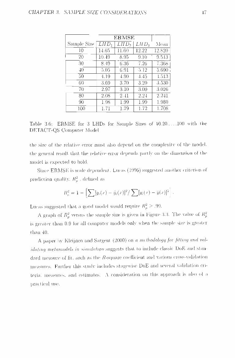
CHAPTER 3. SAMPLE SIZE CONSIDERATIONS
Sample Size 10 20 30 40 50 60 70 80 90 100
E R M S E LHD I 14.65 10.49
8.49 5,05 4.19 3.69 2.97 2.08 1.98 1.71
LHD2 11.60 8.95 6.36 6.91 4.90 3.70 3.10 2.41 1.99 1.79
LHDi 12.22 9.10 7.26 5.12 4.45 3.20 3.00 2.24 1.99 1,72
Mean 12,820 9.513 7.368 5.690 4.513 3.530 3.026 2.241 1.980 1.708
Table 3.6: ERMSE for 3 LHDs for Sample Sizes of 10,20,... ,100 Avith the DETACT-QS Computer Model
the size of the relatiA-e error must also depend on the complexity of the model,
the general result that the relatiA-e error depends partlA- on the dimension of the
model is expected to hold.
Since ERMSE is scale dependent. Lucas (1996) suggested an(-)ther criterion of
prediction c(uality. R^ , defined as
li 1 Y.^y.{-r) yA^- ?lY.^y^[•r)-y[x)f
Lucas suggested that a good model AA'ould require 7? > .99.
A graph of i?^ versus the sample size is giA-en in Figure 3.3. The A-alue of i?p
is greater than 0.9 for all computer models onh' when tlu^ sample size is greater
than 40.
A paper by Kleijnen and Sargent (2000) on a methodology for fitting and val-
idaling metamodels in simulation suggests that to include classic DoE and stan
dard measure of fit, such as the i?-square coefficient and various cross-validation
measures. Further this studA- includes stagewise DoE and several A-aliclation cri
teria, measures, and estimates. A consideration on this approach is also of a
practical use.
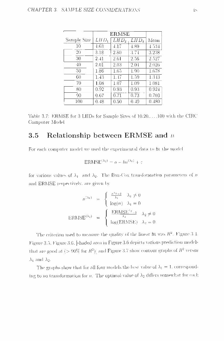
CHAPTER 3. SAMPLE SIZE CONSIDERATIONS 4>s
Sample Size 10 20 30 40 50 60 70 80 90 100
E R M S E LHDi 4.63 3.18 2.41 2,01 1.86 1.43 1.08 0.92 0.67 0.48
LHD2 4.17 2.80 2.61 2.03 1.65 1.47 1.07 0.93 0.71 0.50
LHD-i 4.80 3.74 2.56 2.04 1,90 1.59 1.09 0.93 0.73 0.49
Mean 4.534 3.238 2.527 2.026 1,678 1.343 1.081 0.924 0.703 0.480
Table 3.7; ERMSE for 3 LHDs for Sample Sizes of 10,20,... .100 with the CIRC Computer Model
3.5 Relationship between ERMSE and n
For each computer model Ave used the experimental data to fit the model
ERMSE'^'^) =r/-f/; / ;(^ ')+c-
for A^arious values of Ai and A2. The Box-Cox transformation parameters of
and ERMSE respectiA'el.A-, are given bA-
n
n ^ i - l
n ( A l )
^1 ^ 0 log(n) Ai = 0
ERMSE'2 ERMSE (A2) A2
^ A2 7^0
log(ERMSE) A2 = 0.
The criterion used to measure the quahty of the hnear fit Avas R^. Figure 3.4.
Figure 3.5, Figure 3.6, [shaded area in Figure 3.6 depicts various prediction models
that are good at (> 90% for R^)] and Figure 3.7 SIIOAV contour graphs of R^ \-(>rsus
Al and A2.
The graphs show that for all four models the best \-aIue of Ai = 1, correspond
ing to no transformation for n. The optimal value of A2 differs somcAvhat for each
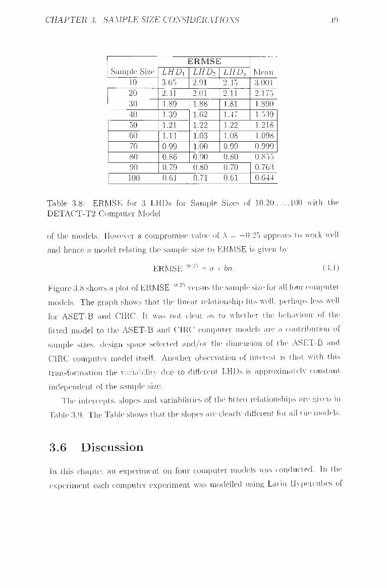
CHAPTER 3. SAMPLE SIZE CONSIDER.\TIONS 49
Sample Size 10 20 30 40 50 60 70 80 90 100
E R M S E LHDi 3.65 2.41 1.89 1.39 1.21 1.11 0.99 0,86 0.79 0.61
LHD2 2.91 2.01 1.88 1,62 1.22 1.03 1.00 0.90 0.80 0.71
LHDi 2.45 2.11 1.81 1.47 1.22 1.08 0.99 0.80 0.70 0.61
Mean 3.001 2.175 1.890 1.539 1.218 1.098 0.999 0.855 0.763 0.644
Table 3.8: ERMSE for 3 LHDs for Sample Sizes of 10,20,... .100 with the DETACT-T2 Computer Model
of the models. HcjAA-e\-er a compromise A-alue of A = -0.25 appears to AA-ork Avell
and hence a model relating the sample size to ERMSE is given by
E R M S E - ° ' ' = a + 6n. (3.1)
Figure 3.8 shoAvs a plot of ERMSE""'^'^ A-ersus the sample sizc> for ah four computer
modefs. The graph shoAvs that the linear relationship fits Avell, perhaps less Avell
for ASET-B and CIRC. It Avas not clear as to Avhether the l)eliaviour of the
fitted model to the ASET-B and CIRC computer models are a contribution of
sample sizes, design space selected and/or the dimension of the ASET-B and
CIRC computer model itself. Another observation of Intercast is that Avith this
transformation the variability due to different LHDs is approximatel\- constant
independent of the sample size.
The intercepts, slopes and variabilities of the fitted relationships are gi\-en in
Table 3.9. The Table shows that the slopes are clearh- different for all the models.
3.6 Discussion
In this chapter an experiment on four computer models Avas conducted. In the
experiment each computer experiment Avas modelled using Latin HA-perculjes of
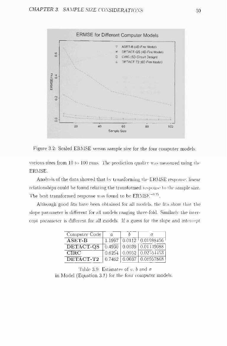
CHAPTER 3. SAMPLE SIZE CONSIDERATIONS 50
CD O
1 ' --E o HI to 2 cr LU
CN O
O O
ERMSE for Different Computer Models
V ASET-B (4D-Fire Model)
y^- DETACT-QS (4D-Ftre Model)
\ • CIRC (5D-Circuit Design)
^ A DETACT-T2 {6D-F)re Model)
^ "
'
~~ i - ^
~ " ~ 'fi- ~ —
— - V TJ.J^ l"^ •** ' » - • I> .... , , ~ • "
20 40 60 80 100
Sample Size
Figure 3.2: Scaled ERMSE A ersus sample size for the four computer models.
A^arious sizes from 10 to 100 runs. The prediction qualitA- was measured using tlic
ERMSE.
Analysis of the data shoAved that by transforming the ERMSE response, linear
relationships could be found relating the transformed resp(-)nse to the sample size.
The best transformed response Avas found to be ERMSE"" '•' ,
Although good fits hav-e been obtained for all models, the fits shoAv that the
slope parameter is different for all models ranging three-fold. Similarh- the inter
cept parameter is different for all models. If a guess for the slope and intercept
Computer Code ASET-B DETACT-QS CIRC DETACT-T2
a 1.1997 0.4930 0.6254 0.7462
b 0.0112 0.0039 0.0052 0.0037
a 0.01988456 0.01449088 0.02554453 0.01957868
Table 3.9; Estimates of a. b and a in Model (Equation 3.1) for the four computer models.
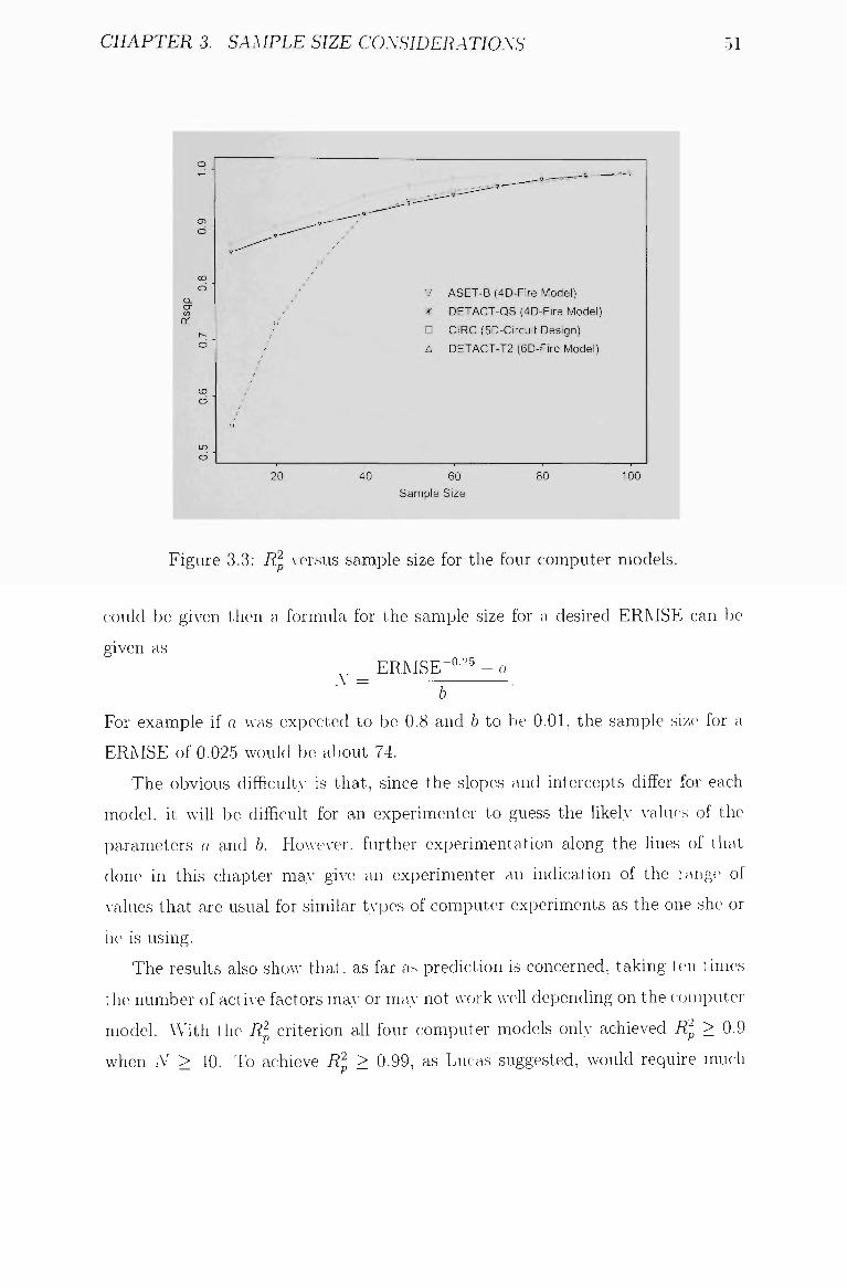
CHAPTER 3. SAMPLE SIZE CONSIDERATIONS 51
o
—
en o -
00
o '
h-
o
(D O "
uo d
^ V — '
V — ^ '
/ /
/ 1
s
1
!
^,^'^-^ ^
V
)i«
D
A
. . - - , - — - ' — = - ^ ' ^'" :::,v-— '
ASET-B (4D-Fire Model)
DETACT-QS {4D-Fire Model)
CIRC (5D-Circuit Design)
DETACT-T2 (6D-Fire Model)
20 40 60 Sample Size
80 100
Figure 3.3; P? Acrsus sample size for the four computer models.
could be giA-en then a formula for the sample size for a desired ERMSE can be
given as
A' ERMSE -0.2.5
For example if a Avas expected to be 0.8 and b to be 0.01, the sample size for a
ERMSE of 0.025 Avould be al)out 74.
The obvious difficuhv- is that, since the slopes and intercepts differ for each
model, it Avill be difficult for an experimenter to guess the likelA- A-alues of the
parameters a and b. HoA\-eA-er, further experimentation along the lines of that
done in this chapter maA- giA e an experimenter an indication of the r^uige of
\-alues that are usual for similar t\'pes of computer experiments as the one she or
li( is using.
The results also sho\A- that, as far as prediction is concerned, taking tc>n times
the number of actiA-e factors may or ma\- not Avork Aveh depending on the computer
model. With the i?^ criterion all four computer models only achieved R\ > 0.9
when N > 40. To achieve /?J > 0.99, as Lucas suggested, Avould require much
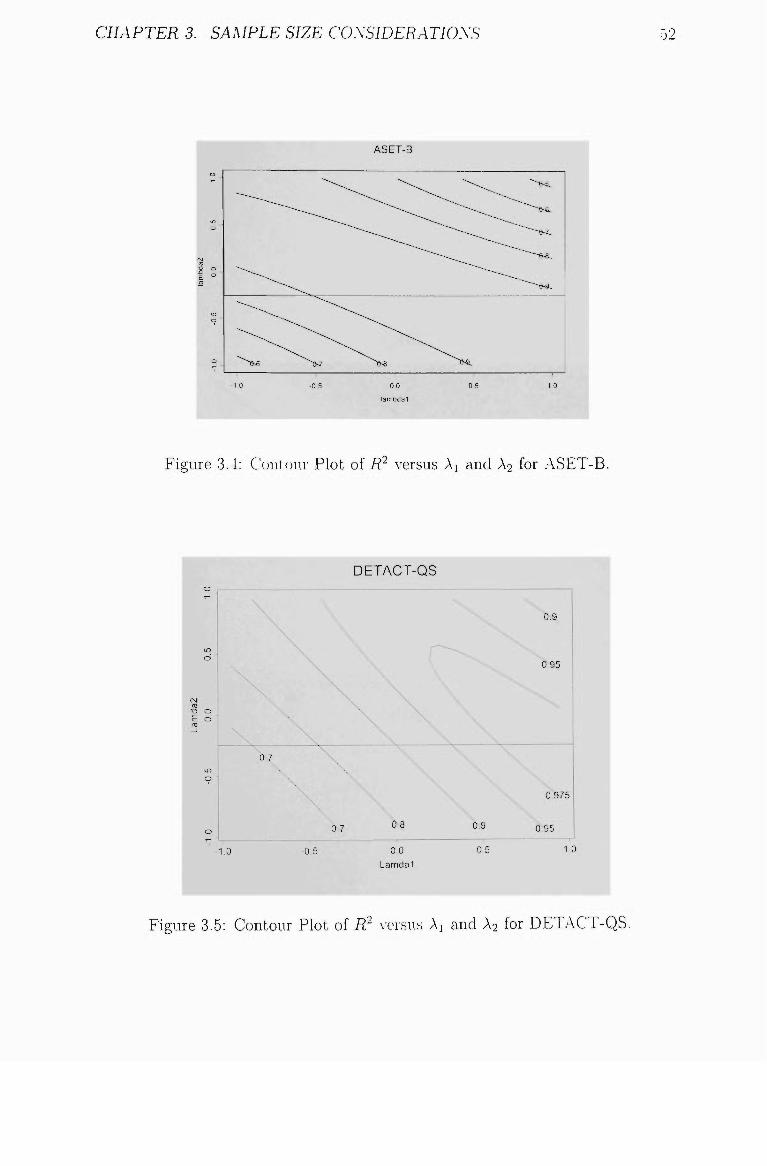
CHAPTER 3. SAMPLE SIZE CONSIDERATIONS
o
d
CM
E °
E °
o
ASET-B
^ ^ T ^ ^ ^ \ : ; ^ . ^ ^
-1.0 -0.5 0,0 0.5 1.0
lambdal
Figure 3.4: Contour Plot of R"^ versus Ai and A2 for ,ASET-B.
DETACT-QS
"D O
e o
-1.0
Figure 3.5: Contour Plot of R^ versus Aj and A2 for DETACT-QS.
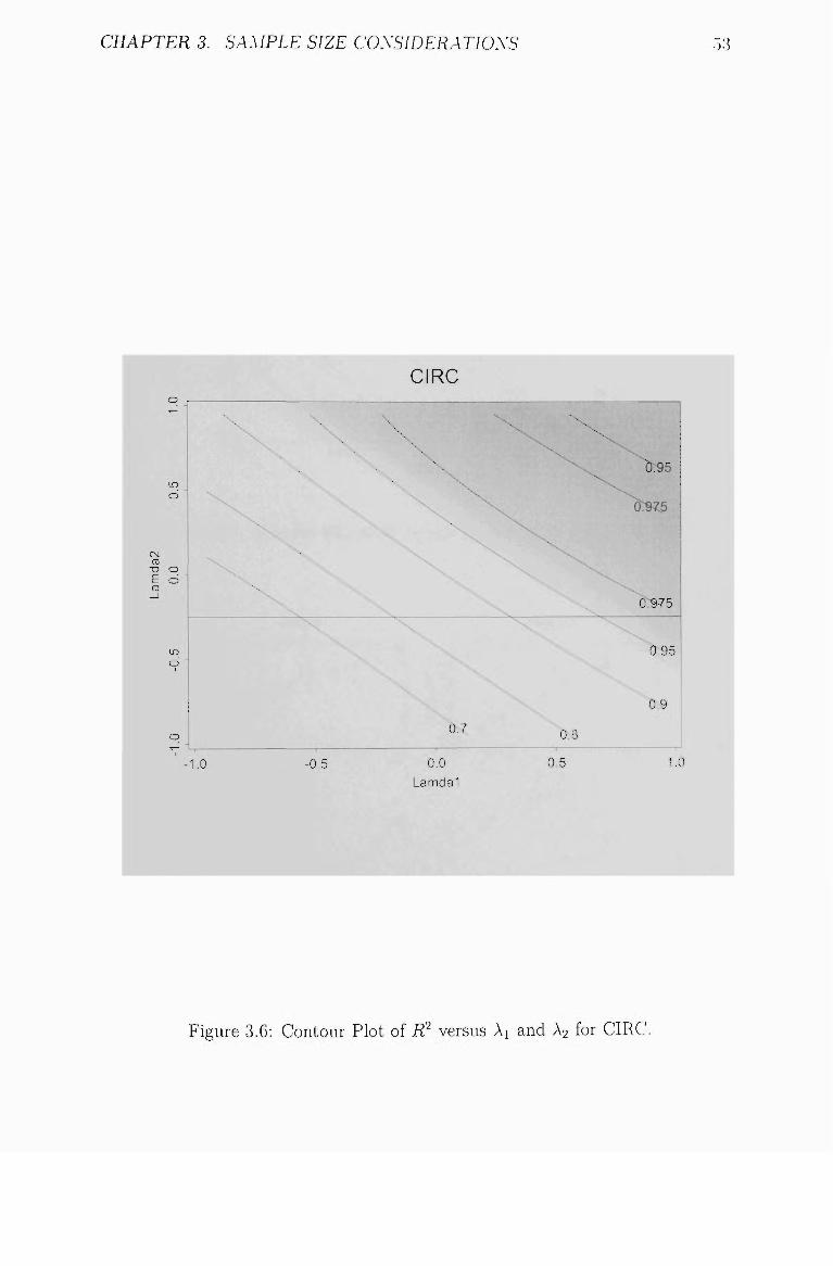
CHAPTER 3. SAMPLE SIZE CONSIDERATIONS
CIRC
O
03 X3 O E O x,
\ ^
\ \ \
X
\
\ ,
• x
• x
\ ^
X ,
^\^
N:8
. . ^ 0:95
07975
0:975
0:95 to o
-1.0 -0.5 0,0
Lamdal
0,5 1.0
Figure 3.6: Contour Plot of R^ versus Ai and A2 for CIRC.
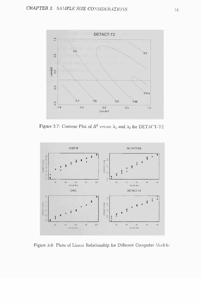
CHAPTER 3. SAMPLE SIZE CONSIDERATIONS 54
La
md
a2
1.0
-0.5
0,
0 0.
5 1.
0
DETACT-T2
6:^ I ^^- - . ^ \ K
^7 ov o>9 oras
10 -0.5 0.0 0 5 1.C
Lamdal
Figure 3.7; Contour Plot of 7? versus Aj and A2 for DETACT-T2.
0
3 ^ UJ to CO ^ 2
lER
2 1.
4
0
• 1
^ "".
^ 0 9 •-
^ oi s =
, 0 1
•
20
• • 20
• •
1
ASET-B
• • 1 •
t
•
40 60
Sample Size
CIRC
. i
40 60
Sample Size
1
•
•
•
80
•
80
t
1
1
100
i
100
_ -
9 ^
« 5 IT
._-
_ ' z ^ ^ ai
5 °
t
• •
t •
20
>
20
• •
t
DETACT-QS
• • m
1 • • •
40 60
Sample Size
DETACT-T2
1 • • t
•
40 60
Sample Size
{
80
* 1
80
• •
100
• • • •
100
Figure 3.8: Plots of Linear Relationship for Different Computer M oclels.

CHAPTER 3. SAMPLE SIZE CONSIDERATIONS • ) • )
greater sample sizes.
In the next chapter the cjuestion of hoAv to augment an experiment AA-IU be
discussed. One application of the relationship found in this chapter will be giA-en
as Avell as some more general methods. As shoAvm in this chapter it is difhcult
to decide on the appropriate size of a computer exi^eriment in acK-ance but if it
is possible to add extra runs then it is possible to control the precision of the
predictions based on the surrogate model.
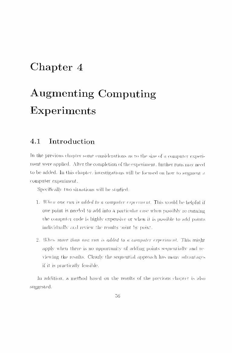
Chapter 4
Augmenting Computing
Experiments
4.1 Introduction
In the previous cha])tcn- some considerations as to the size of a computer experi
ment AAere applied. After the completion of the experiment, hirther runs iiia\- need
to be added. In this chapter, im^estigations will be focused on hoAv to augment a
computer experiment.
Specificalh- tAvo situations AAdll be studied:
1. When one run is added to a computer expernverit. This would be helpful if
one point is needed to add into a particular case u-fien possibly re-running
the computer code is highly expensiA-e or Avhen it is possible to add points
indi\-idually and revicAv the results point bA- point.
2. U7;cn more than one run is added to a computer experiment. This might
applA- Avlien there is no opportunitA' of adding points sequent ialh- and rc>-
\-iewing the results. Clearly the sequential approach has inauA- adx-antages
if it is ])ractically feasible.
In addition, a method based on the results of the prcAaous chapter is also
suggested.
56

CHAPTER 4. AUGMENTING COMPUTING EXPERIMENTS O I
4.2 Adding one run to a computer experiment
After a computer experiment. Ave can generate both a prediction for each point
over the range of interest as weU as the IMSE of the prediction \A-hich describes
how uncertain we are in our prediction. The MSE is zero for the points alread.A-
contained in the computer experiments. A good method for adding a single
run would be to calculate the MSE at each of a potential set of points and
choose the point Avith the maximum MSE. This method is similar to the simple
algorithm developed by Dykstra (1971). The candidate set of points can be
a Latin Hypercube, a grid, am- other Orthogonal Array or Computer Design
or even a Random Set of points over the experimental region. For illustration
purposes a 20 run LHD is used as the initial design and a 10 run LHD as the
candidate set although in practice the candidate set should be much larger than
the initial design.
Table 4.1 gives the coded design points of the initial 20 run LHD with corre
sponding egress times from ASET-B.
Modelling the output as a realization of a stochastic process ga\-e the results
gi\-en in Table 4.2.
Table 4.3 gives the coded candidate points from a 10 run ASET-B again Avith
the corresponding egress times. A pairs plot of the original design points and the
candidate points is giA-en in Figure 4.1.
For each of the candidate points the MSE Avas calculated using Eciuation 2.3.
Note, instead of using the Equation 2.3, by ignoring the random character of the
estimated correlation matrix R and the resulting Kriging Aveights. Kleijnen and
Van Beers (2003) use cross-A-ahdation to estimate the correct A-ariance.
The MSEs are giA-en in the column labelled '1st" in Table 4.4. The candidate
point with the largest MSE is point 6. If this point is added and the model
rehtted the MSEs at the remaining points are giA-en in the column labelled "2ncl"
in Table 4.4. With the result of the additional point 6 added the point Avith the
largest MSE is IIOAV Point 9.
Sometimes it is possible to proceed sequentialh-. The remaining columns of
Table 4.4 giA-e the results \A-hen the process aboA-e is repeated another three times.
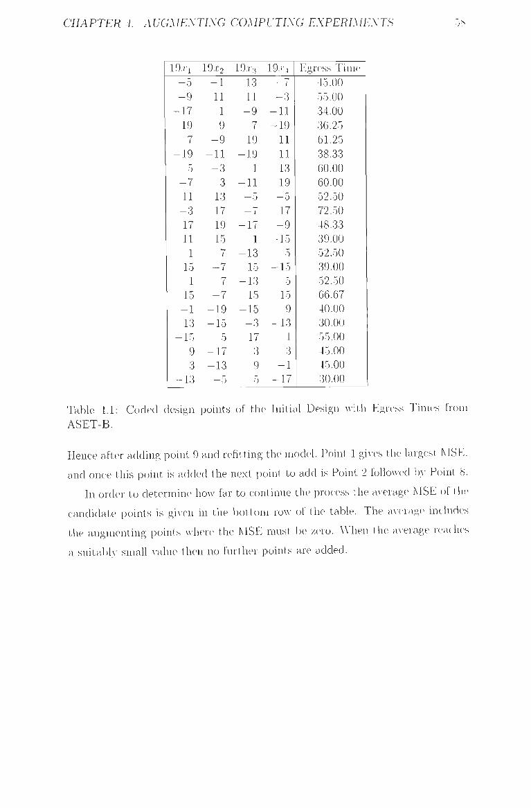
CHAPTER 4. AUGMENTING COMPUTING EXPERIMENTS •jb
19.ri
-5 -9 -17 19 7
-19 5
-7 11 -3 17
-11 1 15 1 15 -1 13
-15 9 3
-13
19X2
-1 11 1 9
-9 -11 -3 3 13 17 19 15 7
-7 7
-7 -19 -15
5 -17 -13 —5
19.r,
13 11 -9 7 19
-19 1
-11 r-
— 0 —7 -17 -1 -13 15
-13 15
-15 -3 17 3 9 5
19./-4
— 7
-3 -11 -19 11 11 13 19 -5 17 -9 -15
5 -15
5 15 9
-13 1 3
-1 -17
Egress Time
45.00
55.00
34.00
36.25
61.25
38.33
60.00
60.00
52.50
72.50
48.33
39.00
52.50
39.00
52.50
66.67
40.00
30.00
55.00
45.00
45,00
30.00
Table 4.1: Coded design points of the Initial Design with Egrc-ss Times from
ASET-B.
Hence after adding point 9 and refitting the modei. Point 1 gives the largest MSE,
and once this point is added the next point to add is Point 2 folloAved bA- Point 8.
In order to determine hoAv far to continue the process the aA-erage MSE of \\\e
candidate points is giA-en in the bottom roAv of the table. The •dxevnge includes
the augmenting points wliere the MSE must be zero. When the aA-erage reaches
a suitabh- small A-alue then no further points are added.
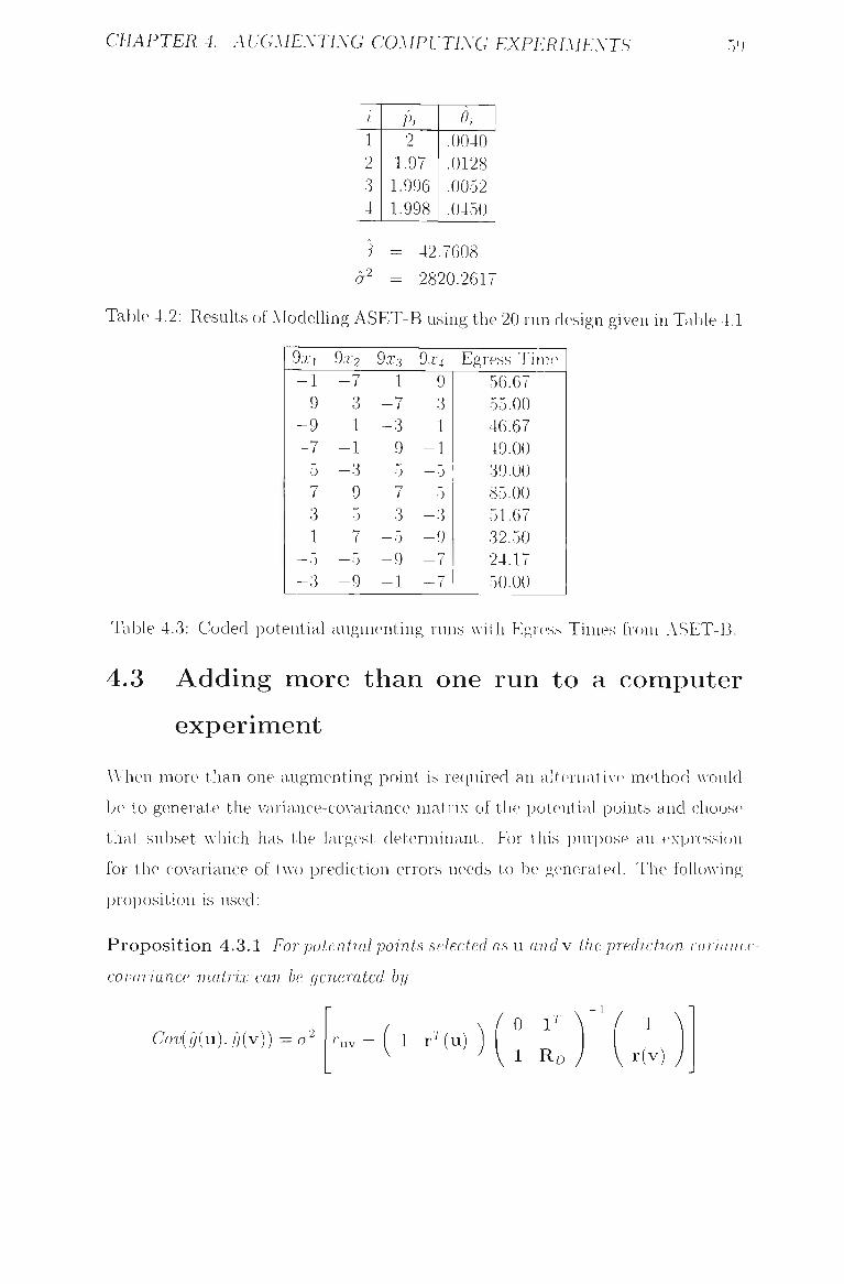
CHAPTER 4. AUGMENTING COMPUTING EXPERIMENTS 59
i 1 2 3 4
3
P, 2
1.97 1.996 1.998
9, .0040 .0128 .0052 .0450
= 42.7608
a^ = 2820,261-
Table 4.2; Results of Modelling ASET-B using the 20 run design given in Table 4.1
9xi
- 1 9
- 9 -1
5 7 3 1
— 5 - 3
9X2 - 7
3 1
- 1 - 3
9 5 7
— 5 - 9
9X3
1 - 7 - 3
9 5 7 3
—5 - 9 - 1
9X4
9 3 1
- 1 - 5
5 - 3 - 9 - 7 - 7
Egress Time 56.67 55.00 46.67 49.00 39.00 85.00 51.67 32.50 24.17 50.00
Table 4.3; Coded potential augmenting runs with Egr(>ss Times from ASET-B.
4.3 Adding more than one run to a computer
experiment
When more than one augmenting point is required an aitc^rnatiA-e method Avould
be to generate the A^ariance-covariance matrix of tiie potential points and choose
that subset A\-hich has the largest determinant. For this purpose an expression
for the covariance of t\\-o prediction errors needs to be generated. The folloAving
proposition is used:
Proposit ion 4.3.1 For potential points selected as u and\' the prediction wrnanc'
cova.Tiance matrix can be generated by
Cov{y{u),y{v))=a' 1 rMu

CHAPTER 4. AUGMENTING COMPUTING EXPERIMENTS 60
-1-0 -0.5 0-0 05 1-0 - 1 0 -0 5 0,0 0 5 10
x1
6 -8
7 2
3 . 4
5 • 9
1 • . • 10 •
2 • 6
5 • . 7
8 • 1
10 • . 9 • •
4 3
x2
. 2 • 8
5 . 7
. 8 1
10 9
• 4 3
6 8 . •
7. • 2-
• . 3 • 4
• 5 • 9
• 1. 10
2 6 •
5 • 7
8 • . . 1
10 • 9
4 • 3 •
6 . 8 •
7 • . "2 3
• 4 5
9 1
• 10
i 9
5 7
1 . • • 10
3 • 8
. 2 9
• .1 10
6 2
3 . 4 .
7 • 5 •
. 9
a
4 • . 6 5
•7 • 1
10 . 3 • •
8 2
9
1 10 • .
6 2
3 . 4
7 • 5
' 9 . • 8
x3
• . 1 1 0 .
6 • • 2 .
3 4
7 5
9 ' • .
a
4 . 6 •
5 7
. 1 10
3 8
2 • 9
x4
1.0
-05
0-0
0
5 1
0 1-
0 -0
-5
0.0
0-5
l-
(
-
-1-0 -0-5 0-0 0 5 1-0 - 1 0 -0 5 0-0 0-5 1 0
Figure 4.1; Original 20 points from a LHD plus 10 labeled candidate points from a 10 run LHD
where the correlation of the zs at u and v is TUV the correlation between the zs
at the design points and at u is
r(u) = [i?(xi, u), 7?(x^, u ix
an d the correlation between the zs at the design points and at v is
r(v) = [ i ? (x i .v ) , . . . , i ? (x„ .v ]T
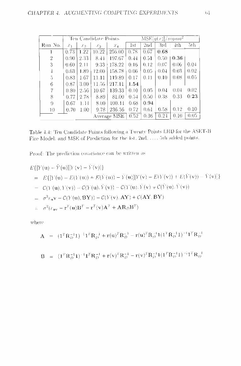
CHAPTER 4. AUGMENTING COMPUTING EXPERIMENTS 61
Run No. 1 2 3 4 5 6 7 8 9 10
Ten Candidate Points •Ti
0.73 0.90 0.60 0.63 0.83 0,87 0.80 0.77 0.67 0.70
• ' • 2
1.22 2.33 2.11 1.89 1.67 3.00 2.56 2.78 1.44
X:i
10.22 8.44 9.33
12.00 11.11 11.56 10.67 8.89 8.00
1.00 9,78
X4
256.00 197.67 178.22 158.78 119.89 217.11 139.33 81.00
100.44 236.56
Average MSE
'MSE[yix)]/signnr 1st
0.78 0.44 0.16 0.06 0.17 1.54 0.10 0.54 0.68 0.72 0.52
2nd 0.67 0,51 0.12 0.05 0.11
0.05 0.50 0.94 0.61 0.36
3rd 0.68 0.50 0.07 0.04 0.10
0.04 0.38
0.58 0.24
4th
0.36 0.06 0.03 0.08
0.04 0.33
0.12 0.10
5tli
0.04 0.02 0.05
0.02 0.23
0.10 0.05
Table 4.4: Ten Candidate Points following a TAvcnitv Pohits LHD for the ASET-B Fire Model: and MSE of Prediction for the 1st, 2nd 5th added points.
Proof: The prediction coA'ariaiicc^ can be Avritten as
E{[Y{u)-Yiu)][Y{v)-Y{v)]}
= E{[Y{n) - E{Y{n)) + EiY{u)) - r (u ) ] [y(v) - E{Y{^)) + E ( r ( v ) )
= c(y(u),r(v))-c(y(u),y(v))-c{v(u).r(v) + c(y(u).r(v))
= <7VuV - C(y(u) , BY)) - C(}-(v), AY) + C(AY, BY)
V(v)]}
= cr r. r ^ 7 u ) B ^ - r ^ ( v ) A ^ + ARz,B^)
Avhere
A l ^ R n 4 ) - ^ l ^ R n ' + r(u)^R "-D D X D - I u)^Rn^lil''Rn'l)''l^R'o' "-D D
B = ( i ^ R B ' i : - l - i X 1' R ^ ' + r (v
iX Rp r (v)^RB4( l '^RB^l)"^ l^Rz
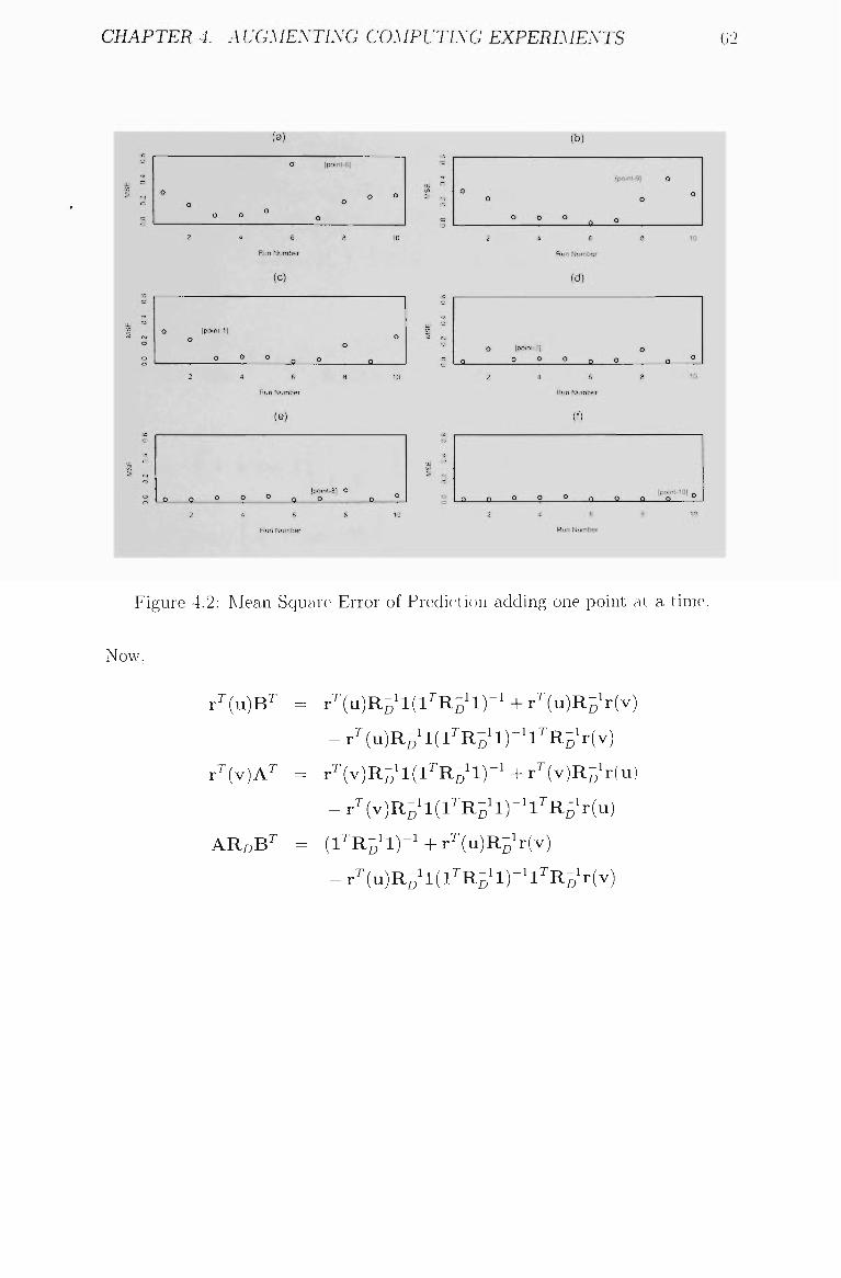
CHAPTER 4. AUGMENTING COMPUTING EXPERIMEXTS ()2
° 2
O
^
^ UJ '^
O
° _r
S CM
o
o
O
O
o o
2
Ipoint-l) 0
O
2
0 ° 2
0
4
O
4
0
4
(a)
0
0
6
Run Number
(c)
° n
6
Run Number
(e)
° 9
Run Number
[poinl-6|
O
o
8
o
o
8
[poinl-81 O O
8
O 0
10
0
10
o
10
LO
MS
E
5
--
-
X
^ o
=
° ^ -N O
o
O O
2
o
2
2
O
Ipoin
O
O
o
4
-21 O
4
O
• "
(b)
O
6
Run Number
(d)
o r>
6
Run Number
(0
O n
Run Number
(pGint-9)
O
o
8
o
o
8
O p
o
[poinl
O
10
o
10
'01 0
Figure 4.2: Mean Squaix^ Error of Prediction adding one point al a I inie.
Now.
r^(u)B^
„Tf,A \T r' V A ' =
ARoB^
r^(u)Ro4( l^RB' l ) -^ + r^(u)RBV(v)
- r^(u)RB^l( l^RB' l ) -4^RB^r(v)
r^(v)R-4( l '^RBH)- ' + r^(v)RBir(u)
- r^fv)R-4(l^^Rn'l)-4^RB^r(u) "•D "•D
l ^RB4) -^+r^ (u )R^ i r (v )
- r^ (u)RB^l ( l^RB4)-4^RBV(v)

CHAPTER 4. AUGMENTING COMPUTING EXPERIMEXTS
Hence,
E{[Y{u)-Y{n)][Y{^r)-Y{v)]}
= o' K v + ( l^RB^l) -^ - r ^ ( u ) R ^ ^ l ( l ^ R - ^ l ) - ^
+ r ^ ( v ) R - 4 ( l ^ R - i l ) - i l ^ R - i r ( u )
- r ^ ( v ) R - i l ( l ^ R - i l ) - i - r ^ ( v ) R - i r ( u ) ] .
- ( l ^ R B ^ l ) - i ( l ^ R B ^ l ) - i l ^ R - ^
RB^l( l^RB^l) -^ RB^ - R - 4 ( l ^ R - 4 ) - ^ l R - ^
a 1 r^(u)
(7- r,.^ - I 1 r^'(u) ) W r(vj
= a' [/„v - ( 1 ^ R : ^ ' 1 ) " ' + r ( u ) R ^ ' l ( l ^ R - 4 ) - ^ + ( l ^ R ^ 4 ) - ^ l ^ R - ' r ( v )
+ r ^ ' » R ^ i r ^ ( v ) - l ^ R B 4 ( l ^ R ^ 4 ) - 4 ^ R - ^ r ( v ) ]
hence proving the result.
Corollary 4.3.1 The prediction varmnce at a site x.
E{[}-(x)-y(x)f}
IS given by
a 1 -- ( ^
r^(x) ) ( ' 0 1^
V 1 R D
1
r(xl
Using this method a number of points could be added at a time. Figure 4.3
gives the determinant of the A'ariance-covariance matrix of the prediction errors
for all sets of hA-e runs out of the ten candidate points from the LHD. In this case
the best set of HA-C points is also the set {1. 2, 6. 8, 9}. Clearly there will be other
cases Avhere the two points axe fitted sequentially. When points are fitted one at
a time the first fiA-e points are {6. 9,1, 2, 8} (see Figure 4.2).

CHAPTER 4. AUGMENTING COMPUTING EXPERIMENTS 64
o
o • ^
Det
erm
inan
t
20
30
o ^
o '. • *. .
0
(1,2,6.8,9)
(1,2,6,9,10)
•
• .
-^^- x.^"-50
(1,6,8,9,10)
••
• .- * f
100 150 Run Combination
•
•
200
•
•
•^ / • '
250
Figure 4.3; Determinant of the A-ariance-coA^ariance matrix of predictions for all possible run combinations of fiA-e runs from the candidate set of 10 runs.
4.4 Another Possible Approach
Eciuation 3.1 giA-es an approximate straight line relationship Ix'tween the
ERMSE"* ' ' and the sample size. The intercept, a. and the slope, b. in the
equation depend on the particular computer model.
The parameters a and b are unknown before the experiment. Assume that
a 2A' -|- 1 run computer experiment is to he conducted. Rather than using a
2A' -f 1 run Latin Hypercube design it might be AA orthwliile using an A run
Latin Flypercube and an A' -|- 1 run Latin Llypercube. Three fits are produced:
one based on the A' run Latin Hypercube, one based on the A' -I- 1 run Latin
Hypercube and one based on the combined design and for each fit the ERMSE is
calculated.
Using the three ERMSE A-alues. linear regression could be used to estimate a
and b, and the sample size sufficient for a particular level of the ERMSE could
be determined. This method ignores the dependence between the ERMSE A-alues
and the fact that neither the combined design nor augmented design are Latin

CHAPTER 4. AUGMENTING COMPUTING ENPERIMENTS 65
Hypercube Designs, but still ma.A' giA e a useful gvudeline to experimenters.
4.5 Discussion
One of the advantages of the method adAocated IDA- Sacks et. al. (1989b) is that
the predictions of the response at untried inputs are accompanied bA- estimates of
the size of the prediction error expected. In this waA- experimenters are informed
as to the usefulness of the predictions.
In cases where the prediction errors are too great, there is the opportunit\-
to improve the predictions by adding extra runs of the computer experiment.
By using such runs the prediction error at the extra runs will be become zero
and in a neighbourhood of the extra runs the error AAUII be small. These extra
runs Avill also haA e an impact on the predictions and their errors elsewhere in the
experimental region.
The question of Avhere to add the extra runs is onc> of practical importance.
Sometimes running the code is just as c^xi)eiisi\-e and time consuming as carrying
out a physical exi)eriment. A number of wa\-s of deciding on the location of the
extra points can be suggested. TAVO such methods liaA-e been examined in this
chapter.
The first method is useful Avhen one point at a time can be added, the results
CA^aluated and then the decision of Avhere the next point can be made. The method
takes as the augmenting point that point which giA-es the maximum prediction
error. This method is easily explained to experimenters since points are adclc cl
where the predictions are AA'orst in terms of size of the prediction error. The
procedure can be continued until the aA-erage or maximum prediction error is
sufficiently small.
If more than one point can be added but there is no opportunitv to cA-aluate
the computer model alter each point then a modification of the first method can
be USCHI. This modification takes the prediction at the point with maximum error
as if it was an actual rc>sult. There is no need to update the maximum likelihood
estimates but the prediction errors should be updated, leading to another point
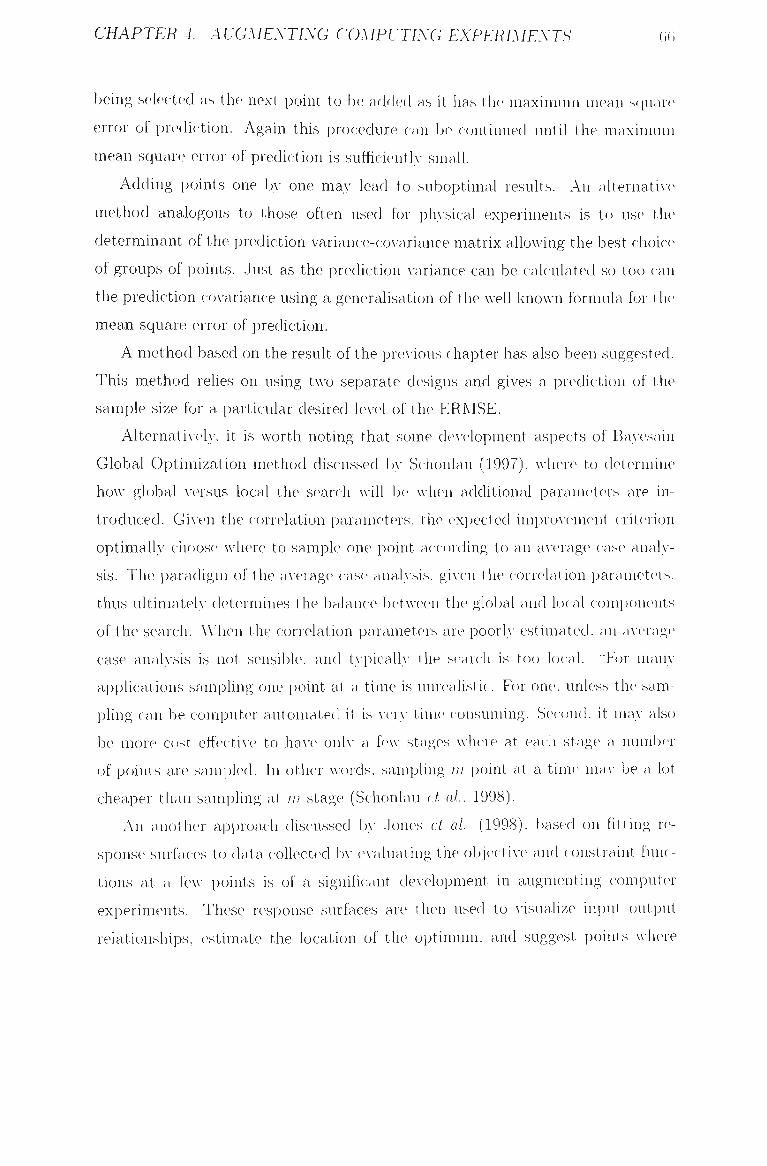
CHAPTER 4. AUGMENTING COMPUTING EXPERIMEXTS GO
being selected as tlie next point to be added as it has the maximum mean scjuare
error of prediction. Again this procedure can be ccmtinued until the maximum
mean square error of prediction is sufficiently small.
Adding points one by one may lead to suboptimal results. An alternatiA-e
method analogous to those often used for pliA'sical experiments is to use the
determinant of the prediction variance-coA^ariance matrix allowing the best choice
of groups of points. Just as the prediction A-ariance can be calculated so too can
the prediction ccjvariance using a generalisation of the well knoAA-n formula for the
mean square error of prediction.
A method based on the result of the previous chapter has also been suggested.
This method relies on using tAvo separate designs and gives a prediction of the
sample size for a particular desired IcA-el of the ERMSE.
Alternatively, it is AA orth noting that some dcA^elopment aspects of BaA-esain
Global Optimization method discussed bA- Schonlau (1997), Avhere to determine
hoAv global A-ersus local the search will be when additional parameters are in
troduced. GiA-en the correlation parameters, the expected improvement criterion
optimally choose Avhere to sample one point according to an aA-erage case analy
sis. The paradigm of the aA-erage case analA-sis, giA-en the correlation parameters,
thus ultimatefA' determines the balance l:ietweeii the global and local components
of the search. When the correlation parameters are poorly estimated, an aA-erage
case anal\-sis is not sensible, and t>-picallA- the search is too local. -For many
applications sampfing one point at a time is unrealistic. For one. unless the sam
pling can be computer automated it is vevy time consuming, Sc-cond. it maA- also
be more cost eff'ectiA-e to haA-e onh- a few stages Avhere at each stage a number
of points are sampled. In other Avords, sampling in point at a time maA- be a lot
cheaper than sampling at m stage (Schonlau et al, 1998).
An another approach discussed by Jones et al (1998), based on fitting re
sponse surfaces to data collected IJA- CA-aluating the objectiA-e and constraint func
tions at a lew- points is of a significant development in augmenting computer
experiments. These response surfaces are then used to Aisuafize input output
relationships, cvstimate the location of the optimum, and suggest points where

CHAPTER 4. AUGMENTING COMPUTING EXPERIMENTS 67
additional function evaluations may help improA-e this c^stimate. This approach
not only provides an estimate of the optimal point, but also facihtates the de
velopment of intuition and understanding about what is going on in the model
(Jones et al, 1998),
Finally, a method developed on the leave-one-oid approach employed by Klei
jnen and van Beers (2003) to estimate the true I/O function through cross —
validation is worth noting. In this approach, the authors obtained estimation of
the imcertainty of output at input combinations not A-et observed, b.A- successiA-ely
deleting one of the I/O observations already simulated. For more information
on cross-validation see Stone (1974) and for an update see Meckesheimer et al.
(2002) and Mertens (2001).

Chapter 5
A Model for Computer Models
5.1 Introduction
Computer Experiments, consisting of a number of runs of a computer model with
different inputs, are now commonplace in scientific research. Based on running
the computer model at a set of conditions, a surrogate model can be built to give
a good approximation to the output of the computer model at untried inputs.
The ciualitA- of the prediction depends on the sample size of the experiment and
the complexitA- of the computer model.
This chapter describes an experiment on this proct^ss. The inputs of the
computer experiment are the paranu^ters that describe the c(-)mplexit\- of the
computer model and, the sample size and the output is the empirical mean square
error of the prediction of the fitted surrogate computer model. The results show
how the sample size of the experiment and complexity of the computer model
imi)acl on the prediction c[uahty of the surrogate computer model.
5.2 Simulating ASET-B
In Chapter 2 the ASET-B computer model was introduced. A 50 run computer
experiment \\-a.s conducted and the parameters of the surrogate computer model,
using the methodology of Sacks et al (1989b), Avere estimated.

CHAPTER 5. A MODEL FOR COMPUTER MODELS ()9
n 10
30
50
70
a' 1
123,556 1
123.556
1 123.556
1
123.556
In(EMSE) -5.435 -0.810
-8.800 -2.846
-8.989 -4.351
-10,518 -5.261
-7.126 -0.275 -8.912
-4.279
-9,436 -5,294
-9.926 -5.604
-6.932
-1.060
-8.469 -4.030
-9.763 -4.750
-10.748 -5.886
-5.764
-1.070
-8.910 -3.442
-8.944
-4.581
-10.591 -5.590
-6.460 -1.099 -8.467 -3.591
-9.768 -4.667
-10.749 -5.511
Table 5.1; Results for experiment on surrogate ASET-B model.
In Chapter 3 an experiment on the ASET-B computer model, as Avell as three
other computer models, was conducted. In the experiment the sample size was
varied from 10 to 100 runs and the Empirical Root Mean Square Error of the
fitted surrogate computer models Avas found.
In this section a similar experiment to that cjf chapter 3 AA-IU be conductcnl
using the surrogate computer model. TAVCJ sets of simulations Avill be conducted.
In the first set the 9 and p parameters found in Table 2.9 Avill be used to estimate
the A'aria,nce-co\-ariance matrix of the stochastic process assuming the underh-ing
variance is 1. The Choleski decomposition of t he variance-coA-ariance matrix Avill
be used to generate the obserA^ations. In the second set of simulations the same
procedure will be used but Avith the A-ariance set equal to the estimate gi\-eii in
Table 2.9, i.e a^ = 123.556.
For sample sizes of 10, 30, 50 and 70 fiA-e Latin Ih-percube Designs Avere
generated for each set. For each Latin Hypercube the responses were generated
using parameters of the fitted surrogate computer model. The methodology of
Sacks et al (1989b) Avas used to fit a surrogate computer model to the data
and 1000 random check points over the experimental region were used so that,
the empirical mean square error could be calculated. The results are giA-en in
Table 5.1 and Figure 5.1.
The results shoAv good agreement between the simulated A-alues in Tabl(> 5.1
and the actual \-alues as given in Table 3.5. In addition TaV)ie 5.1 indicates thai
simulating Avith a^ = 1 is sufficient since the average difference iii log(EMSE)
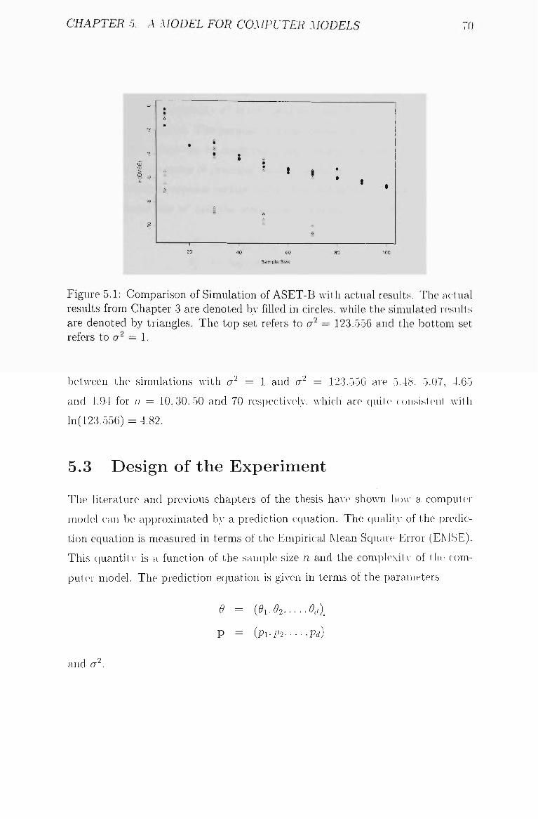
CHAPTER 5. A MODEL FOR COMPUTER MODELS
•ft
LU ^ _
<o _
o
• • •
. ' » 1 •
• • .
i
20 40 60 80 100
Sample Size
Figure 5.1; Comparison of Simulation of ASET-B with actual results. The actual results from Chapter 3 are denoted by filled in circles. Avhile the simulated results are denoted by triangles. The top set refers to cr = 123.556 and the bottom set refers to cr = 1.
betAA een the simulations with a^ = I and cr = 123.556 are 5.48. 5.07, 4.65
and 4.94 for n = 10,30,50 and 70 respectivelA-. which are quite consistent with
ln(123.556) = 4.82.
5.3 Design of the Experiment
The literature and previous chapters of the thesis ha\-e shoAvn how a computer
model can be approximated by a prediction eciuation. The ciualit\- of the predic
tion eciuation is measured in terms of the Empirical Mean Square Error (EMSE).
This c|uantit,A- is a function of the sanipie size n and the complexity of the com-
putc>r model. The prediction ecjuation is giA-en in terms of the parameters
e = {9i.e2.....0d).
P = {Pl-P2----.Pd)
and 0" .
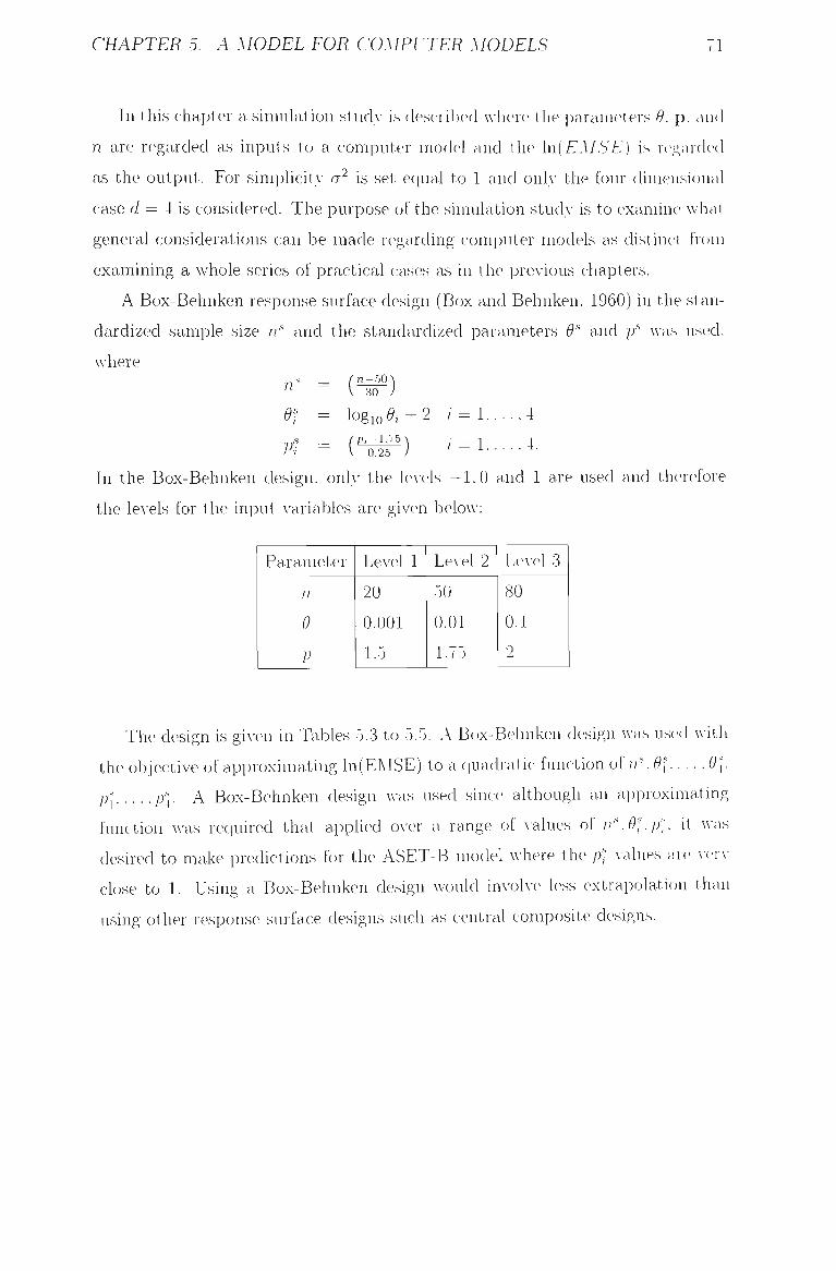
CHAPTER 5. A MODEL FOR COMPUTER MODELS 71
In this chapter a simulation study is described Avhere the parameters 9. p. and
n are regarded as inputs to a computer model and the ln(£'-U.S'£') is regarded
as the output. For simplicity a'^ is set equal to 1 and onl}- the four dimensional
case d = i\s considered. The purpose of the simulation stud}- is to examine Avhat
general considerations can be made regarding computer models as distinct from
examining a whole series of practical cases as in the previous chapters.
A Box-Behnken response surface design (Box and Behnken, 1960) in the stan
dardized sample size r?'' and the standardized parameters 0-'^ and p'^ was used.
Avhere
" ' = ( T i ? ) 0f = logioe, + 2 , = l-----4
Pi = i ' - ^ ) ' = 1 J-
In the Box-Behnken design, only the ICACIS - 1 , 0 and 1 are used and therefore
the levels for the input A-ariables are given beloAv:
Parameter
//
9
P
Level 1
20
0.001
1.5
LcA-el 2
50
0.01
1.75
Level 3
80
0.1
2
The design is giA-en in Tables 5.3 to 5.5. A Box-Behnken design was used Avith
the objective of approximating In(EMSE) to a c|uadratic function of n".0-l 9^,
PI p'l. A Box-Behnken design Avas used since although an approximating
function was required that applied over a range of A-alues of n',0l,p'i. it \\-as
desired to make predictions for the ASET-B model AAJiere the p' A-alues are A-erA-
close to 1. Using a Box-Behnken design would invoh-e less extrapolation than
using other response surface designs such as centrat composite designs.
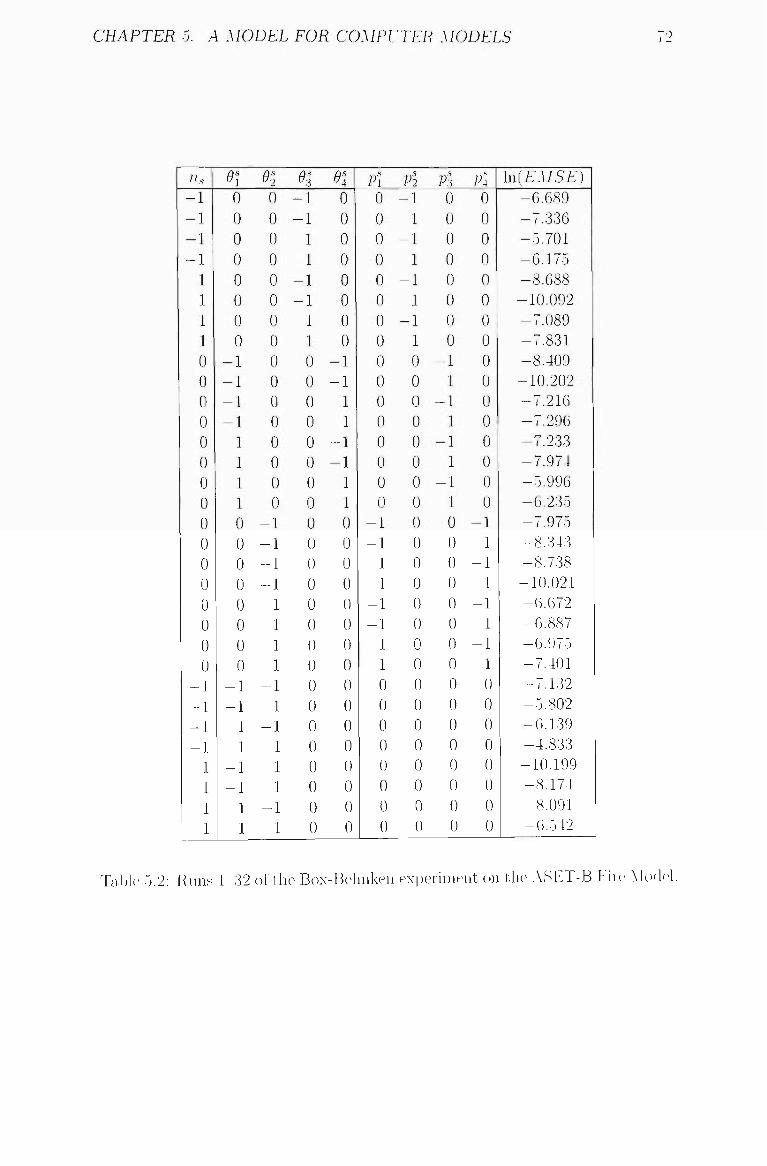
CHAPTER 5. A MODEL FOR COMPUTER MODELS
n.. - 1 - 1 - 1 - 1
1 1 1 1 0 0 0 0 0 0 0 0 0 0 0 0 0 0 0 0
- 1 - 1 - 1 - 1
1 1 1 1
9t 0 0 0 0 0 0 0 0
- 1 - 1 - 1 - 1
1 1 1 1 0 0 0 0 0 0 0 0
- 1 - 1
1 1
- 1 - 1
1 1
0-^ 0 0 0 0 0 0 0 0 0 0 0 0 0 0 0 0
- 1 - 1 - 1 - 1
1 1 1 1
- 1 1
- 1 1
- 1 1
- 1 1
^3
- 1 - 1
1 1
- 1 - 1
1 1 0 0 0 0 0 0 0 0 0 0 0 0 0 0 0 0 0 0 0 0 0 0 0 0
01 0 0 0 0 0 0 0 0
- 1 - 1
1 1
- 1 - 1
1 1 0 0 0 0 0 0 0 0 0 0 0 0 0 0 0 0
Pi 0 0 0 0 0 0 0 0 0 0 0 0 0 0 0 0
- 1 - 1
1 1
- 1 - 1
1 1 0 0 0 0 0 0 0 0
Pi - 1
1 - 1
1 - 1
1 - 1
1 0 0 0 0 0 0 0 0 0 0 0 0 0 0 0 0 0 0 0 0 0 0 0 0
Ps 0 0 0 0 0 0 0 0
- 1 1
- 1 1
- 1 1
- 1 1 0 0 0 0 0 0 0 0 0 0 0 0 0 0 0 0
Pi 0 0 0 0 0 0 0 0 0 0 0 0 0 0 0 0
- 1 1
- 1 1
- 1 1
- 1 1 0 0 0 0 0 0 0 0
HEMSE) -6.689 -7.336 -5.701 -6.175 -8.688 -10.092 -7.089 -7,831 -8.409 -10.202 -7.216 -7.296 -7.233 -7.974 -5.996 -6.235 -7.975 -8.343 -8.738
-10.021 -6.672 -6.887 -6.975 -7.401 -7.132 -5.802 -6.139 -4.833 -10.199 -8.174 -8.091 -6.542
Table 5.2: Runs 1 32 of the Box-Behnken experiment on the ASET-B Fire Model.
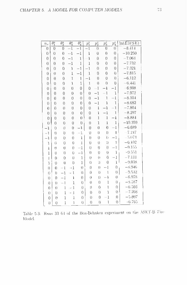
CHAPTER 5. A MODEL FOR COMPUTER MODELS
n,5
0 0 0 0 0 0 0 0 0 0 0 0 0 0 0 0
- 1 - 1 - 1 - 1
1 1 1 1 0 0 0 0 0 0 0 0
01 0 0 0 0 0 0 0 0 0 0 0 0 0 0 0 0 0 0 0 0 0 0 0 0 0 0 0 0 0 0 0 0
0^2 0 0 0 0 0 0 0 0 0 0 0 0 0 0 0 0 0 0 0 0 0 0 0 0
- 1 - 1 - 1 - 1
1 1 1 1
01 -1 - 1 - 1 - 1
1 1 1 1 0 0 0 0 0 0 0 0 0 0 0 0 0 0 0 0
- 1 - 1
1 1
- 1 - 1
1 1
01 - 1 - 1
1 1
- 1 - 1
1 1 0 0 0 0 0 0 0 0
- 1 - 1
1 1
- 1 - 1
1 1 0 0 0 0 0 0 0 0
Pi - 1
1 - 1
1 - 1
1 - 1
1 0 0 0 0 0 0 0 0 0 0 0 0 0 0 0 0 0 0 0 0 0 0 0 0
Pi 0 0 0 0 0 0 0 0
- 1 - 1 - 1 - 1
1 1 1 1 0 0 0 0 0 0 0 0 0 0 0 0 0 0 0 0
Pi 0 0 0 0 0 0 0 0
- 1 - 1
1 1
- 1 - 1
1 1 0 0 0 0 0 0 0 0
- 1 1
- 1 1
- 1 1
- 1 1
Pi 0 0 0 0 0 0 0 0
- 1 1
- 1 1
- 1 1
- 1 1
- 1 1
- 1 1
- 1 1
- 1 1 0 0 0 0 0 0 0 0
\n{EMSE) -8.414
-10.250 -7.064 -7.732 -7.321 -7.815 -6,112 -6.441 -6,908 -7.972 -8.104 -8,682 -7.804 -8.297 -8.884 -10.359 -6.689 -7.247 -5.073 -6.102 -9.155 -9.551 -7.111 -9.038 -8.946 -9.532 -6.978 -8.587 -6.503 -7.208 -5.807 -6.765
Table 5.3; Runs 33 64 of the Box-Behnken experiment on tlie ASET-B Fhe
Model.
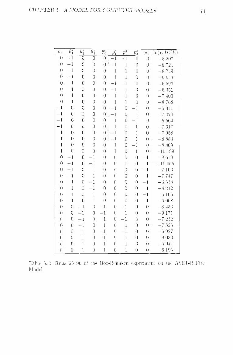
CHAPTER 5. A MODEL FOR COMPUTER MODELS
Us
0 0 0 0 0 0 0 0
- 1 - 1 - 1 - 1
1 1 1 1 0 0 0 0 0 0 0 0 0 0 0 0 0 0 0 0
91 - 1 - 1 - 1 - 1
1 1 1 1 0 0 0 0 0 0 0 0
- 1 - 1 - 1 - 1
1 1 1 1 0 0 0 0 0 0 0 0
01 0 0 0 0 0 0 0 0 0 0 0 0 0 0 0 0 0 0 0 0 0 0 0 0
-1 - 1 - 1 - 1
1 1 1 1
^.3
0 0 0 0 0 0 0 0 0 0 0 0 0 0 0 0
- 1 - 1
1 1
- 1 - 1
1 1 0 0 0 0 0 0 0 0
01 0 0 0 0 0 0 0 0 0 0 0 0 0 0 0 0 0 0 0 0 0 0 0 0
- 1 - 1
1 1
- 1 - 1
1 1
Pi - 1 - 1
1 1
- 1 - 1
1 1
- 1 - 1
1 1
- 1 - 1
1 1 0 0 0 0 0 0 0 0 0 0 0 0 0 0 0 0
Pi - 1
1 - 1
1 - 1
1 - 1
1 0 0 0 0 0 0 0 0 0 0 0 0 0 0 0 0
- 1 1
- 1 1
- 1 1
- 1 1
Pi 0 0 0 0 0 0 0 0
- 1 1
- 1 1
- 1 1
- 1 1 0 0 0 0 0 0 0 0 0 0 0 0 0 0 0 0
Pi 0 0 0 0 0 0 0 0 0 0 0 0 0 0 0 0
- 1 1
- 1 1
- 1 1
- 1 1 0 0 0 0 0 0 0 0
HEMSE) -8.307 -8.721 -8.749 -9.943 -6.599 -6.351 -7.400 -8.768 -6.341 -7.070 -6.664 -7.617 -7.958 -8.883 -8.869
-10.189 -8.650
-10.065 -7.106 -7.747 -6.538 -8.242 -6.106 -6.068 -8.456 -9.171 -7.232 -7.825 -6.927 -9.033 -5.947 -6.195
Table 5.4: Runs 65 96 of the Box-Behnken experiment on the ASET-B Fire Model.
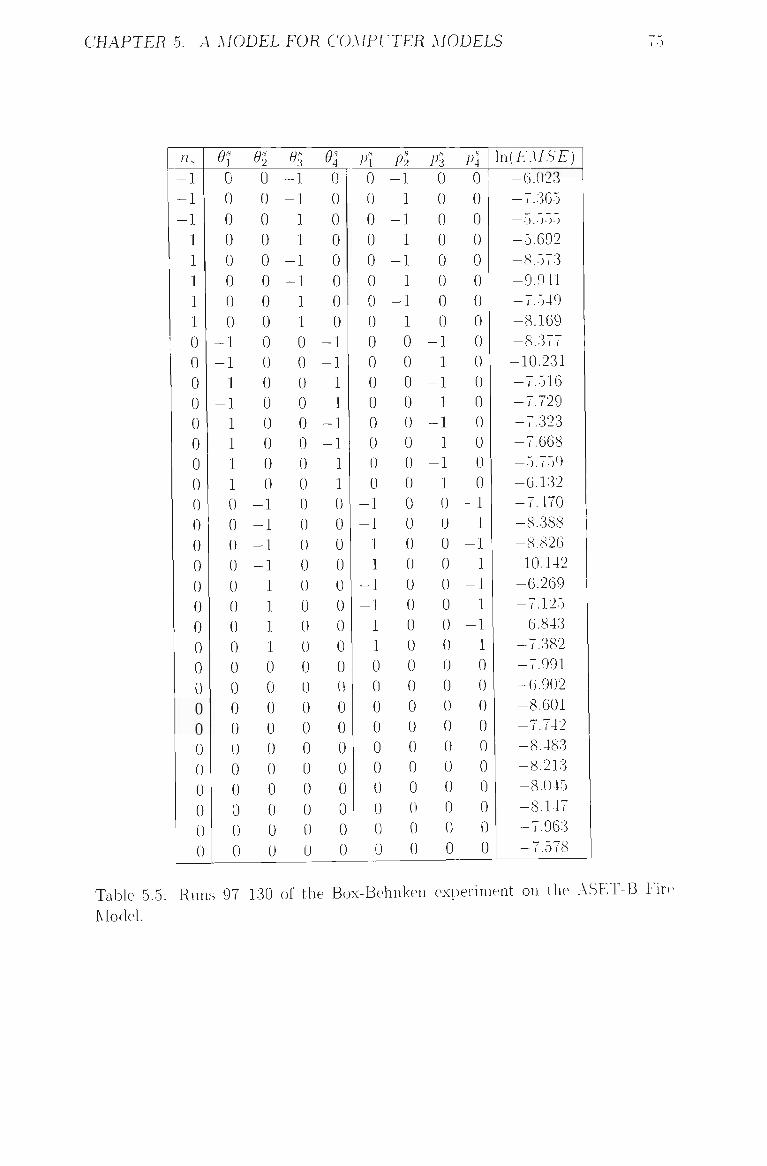
CHAPTER 5. A MODEL FOR COMPUTER MODELS I -J
n.s - 1 - 1 - 1 - 1
1 1 1 1 0 0 0 0 0 0 0 0 0 0 0 0 0 0 0 0 0 0 0 0 0 0 0 0 0 0
01 0 0 0 0 0 0 0 0
- 1 - 1 - 1 - 1
1 1 1 1 0 0 0 0 0 0 0 0 0 0 0 0 0 0 0 0 0 0
1 0 0 0 0 0 0 0 0 0 0 0 0 0 0 0 0
- 1 - 1 - 1 - 1
1 1 1 1 0 0 0 0 0 0 0 0 0 0
o-s - 1 - 1
1 1
- 1 - 1
1 1 0 0 0 0 0 0 0 0 0 0 0 0 0 0 0 0 0 0 0 0 0 0 0 0 0 0
01 0 0 0 0 0 0 0 0
- 1 - 1
1 1
- 1 - 1
1 1 0 0 0 0 0 0 0 0 0 0 0 0 0 0 0 0 0 0
Pl 0 0 0 0 0 0 0 0 0 0 0 0 0 0 0 0
- 1 - 1
1 1
- 1 - 1
1 1 0 0 0 0 0 0 0 0 0 0
Pl - 1
1 - 1
1 - 1
1 - 1
1 0 0 0 0 0 0 0 0 0 0 0 0 0 0 0 0 0 0 0 0 0 0 0 0 0 0
Pl 0 0 0 0 0 0 0 0
- 1 1
- 1 1
- 1 1
- 1 1 0 0 0 0 0 0 0 0 0 0 0 0 0 0 0 0 0 0
Pl 0 0 0 0 0 0 0 0 0 0 0 0 0 0 0 0
- 1 1
- 1 1
- 1 1
- 1 1 0 0 0 0 0 0 0 0 0 0
IniEMSE) -6.023 -7.365 —5.555 -5.692 -8.573 -9.941 -7.549 -8.169 -8.377
-10.231 -7.516 -7.729 -7.323 -7.668 -5.759 -6.132 -7.470 -8.388 -8.826 -10.142 -6.269 -7.125 -6.843 -7.382 -7.991 -6.902 -8.601 -7.742 -8.483 -8.213 -8.045 -8.147 -7.963 -7.578
Table 5.5: Runs 97 130 of the Box-Behnken experiment on the ASET-B Fire
Model
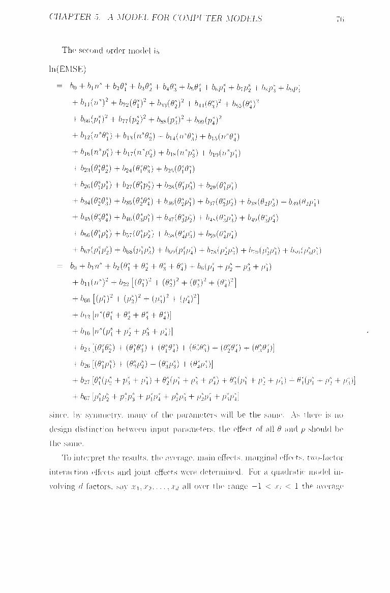
CHAPTER 5. A MODEL FOR COMPUTER MODELS 76
The second order model is
In(EMSE)
= 60 + 61 n' + b20l + bs0-^ -f b40-l + b^,9-l + h^p\ + 67PI + 6si/.; + b^pl
+ 6n(n')2 + 622(^0' + hsiOlY + h44{0^ + h,,{0l)^
+ h,{p\)^ + 677(p|)' + 688(p; )2 + b,,{pl)^
+ 6i2(n-'^J) + 6i3(n-'^^) + b^n'Ol) + 6i5(n^^^)
+ 6i6(nVi) + 6i7(n^p^) + 6i8(7i-'p: ) + b^.in'pl)
+ h2i{0{0'2) + h24{0l0l)+b2,{0\Ol)
+ 6 2 6 ( « ) + b27{0\pl) + ^28(^?P|) + b2,{0\lf4)
+ 6:34( 2 .1) + 63.5( ^^ ) + 636(^^PD + 637(^|P|) + ^38(^2P|) + 639(^,/;l)
+ 645( 1 ) + h^Mp]) + 647( 1 1) + 64s(^K) + h^iOlpl)
+ 6.56(^4^0 + h-{0lpl) + 6.58(^1P|) + b,,{9lpl)
+ ^67(PlP2) + 668(Plp|) + 669(Pi/^I) + 678(P2P|) + '>7',(/4P1) + ^SOI/'^PD
= 60 + 6in' + 62(^1 +02 + 91 + 4') + K{p\ + p | + p | + P4)
+ 6n(rr^)2 + 622 [{91)' -f (^^)^ + m ' + (^,')2]
+ &66 [ ( P D ' + (P2) '+ ( p i r + ( P D ' ]
-f6i2[n^(^? + ^^ + ^ | + ^D]
+ 6 i6[n^(p ' J - fp^+p |+ /;!)]
+ 623 ,[( ^ 2') + (^1^3) + ( 1^4') + (^2^3) + {0-101) + {0Wi)\
+ ^ 2 6 [ ( « ) + (^|p|) + ( « ) + (^lpl)]
+ 27 mih + Pl + Pl) + ^2(P; + Pl + Pl) + ^l(Pl +P2+lh)+ Ol{pl +J4+ /;^)]
+ 67 [PIP2 + PlPs + PIPI + PIPI + P2PI + PIPI]
since, by sA-mmetrA-, niauA- of the parameters AAUU be the same. As there is no
design distinction betAA-een input parameters, the effect of all 9 and p should be
the same.
To interpret the results, the aA-erage, main effects, marginal effects, tA\-(;-factor
interaction (effects and joint effects Avere determined. For a quadratic model in-
A^olving d factors, say Xi , . r2 , . . . , .r,/ all OAer the range — 1 < x, < 1 the a\-erage

CHAPTER 5. A MODEL FOR COMPUTER MODELS
> summaryCfourdcasefit, cor = F)
Coefficients:
(Intercept)
Value Std.Error T-Stat
-8.0665 0.0900 -89.6048
ns
I(thls+th2s+th3s+th4s)
I(pls+p2s+p3s+p4s)
I(ns~2)
I(thls"2+th2s"2+th3s^2+th4s"2)
I (pls"2-^p2s"2+p3s"2+p4s^2)
I(ns*(thls+th2s+th3s+th4s))
I(ns*pls+ ... -ns*p4s)
I(thls*pls+ ... +th4s*p4s)
-1.1062 0.0450
0.7725 0.0225
-0.4421 0.0225
0.3886 0.0581
0.2950 0.0375
-0.0955 0.0375
0.1169 0.0450
-0.1095 0.0450
-0.1899 0.0503
I(thls*(p2s+p3s+p4s)+th4s*(pls+p2s+p3s)) 0.1731 0.0244
I(thls*th2s+thls*th3s+th3s*th4s)
I(pls*p2s+pls*p3s+p3s*p4s)
-0.0884 0.0380
-0.1121 0.0380
Residual standard error: 0.2847 on 117 degrees of freedom Multiple R-Squared: 0.9536 F-statistic; 200.2 on 12 and 117 degrees of freedom, the p-value is 0
-24.5754
34.3237
-19,6438
6.6868
7.8765
-2.5494
2.5982
-2.4327
-3.7743
7.0906
-2.3226
-2.9479
Table 5.6: Results for the Bpx-Behnken design on the ASET-B Computer Model

CHAPTER 5. A MODEL FOR COMPUTER MODELS
over the region is giA-en \)\
x.e[-i,i] ^ ' ' '<J' ^
«"+3 (!]''"]
Similarly, the main effect of x^ over the region is giA-en b\-
f-J'k{Xk) = n / " • / I ^0 + ^ a,Xi + ^ a„.T^ + Y^ a,jX,Xj j J J c/.r, - po
ao + afcXfc + afc/ca: + r I 2_^ «» ) - Po
i-^k
2 1
a/cXfc -|- afcfc.u — -C/AA-.
The marginal effect of x^ is giA-en bA-
Mo + t^k{->-k)
o 1 ao + (H-x^. + aH-n <l~)
Also, the interaction effect of x^ and Xi is giA-en l-)\-
M-r,. X,) = Jz^ [ ••• f i(^o + J2 "'• •' + Z «"•'•' + Z '^'r'-'-'-J n ^ •'•' x, :^fc , /e[- l , l
-/'A-(-Tfc) - Pi{-ri) - PQ
= Oo + OA-.T/,. -F O/.T, + a/ -A-.r , + auxj + c/A./.r/,,.r,
Finally, the joint effect of x^ and x, is giA-en b,A-
po + pk{rk) + /'/(.r/) + likiii-'k, -n)
^ (S")" .2 ao + - 1 2_. a,;j 1 -f cikXk + o.}X, + Okk'-^-k + '-'n'-^'i + "kfJ-k-ll-
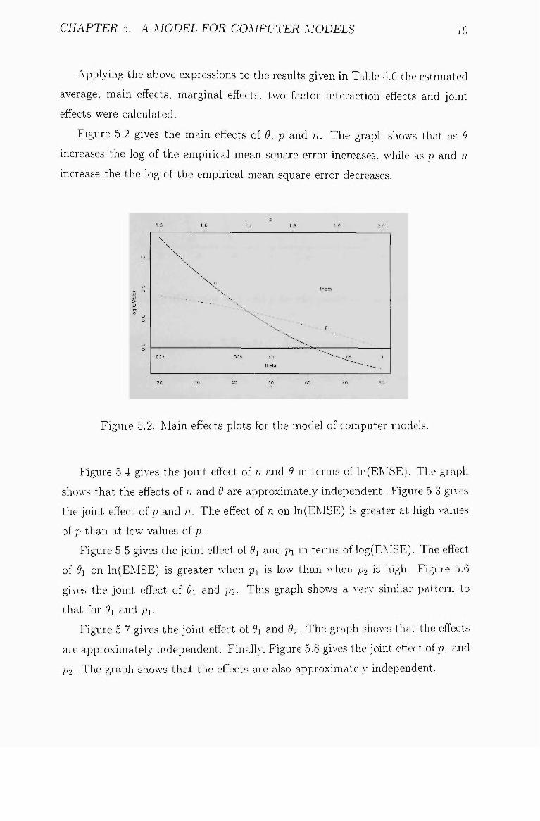
CHAPTER 5. A MODEL FOR COMPUTER MODELS 79
Applying the aboA e expressions to the results given in Table 5.0 the estimated
average, main effects, marginal effects, IAVO factor interaction effects and joint
effects were calculated.
Figure 5.2 gives the main effects of 9. p and n. The graph shoAvs tliat as 0
increases the log of the empirical mean square error increases, Avhile as p and /;
increase the the log of the empirical mean square error decreases.
Figure 5.2: Main effects plots for the model of computer models.
Figure 5.4 gives the joint effect of n and 9 in ieims of ln(El\ISE). The graph
shoAvs that the effects of n and 9 are approximately independent. Figure 5.3 giA-es
the joint effect of p and n. The effect of n on In(EMSE) is greater at high A-alues
of p than at IOAV values of p.
Figure 5.5 gives the joint effect of 9-i and pi in terms of log(EMSE). The effect
of 9x on In(EMSE) is greater when pi is low than Avhen p2 is high. Figure 5.6
giA-es the joint effect of 9i and po- This graph shows a A-ery similar pattern to
that for 9i and pi.
Figure 5.7 gives the joint effect of 9i and ^2- The graph shoAA-s that the effects
are approximately independent. Finally, Figure 5.8 gives the joint effect of pi and
po. The graph shows that the effects are also approximateh- independent.

CHAPTER .5. A MODEL FOR COMPUTER MODELS ^0
Figure 5.3: Joint effect plot of n and p for the model of computer models.
5.4 A Computer Model Approach
Rather than analyse the data using a quadratic approximation, an alternatiA-(>
approach is to model the output, in this case the natural logarithm of the EMSE.
as a function of the input parameters: JI.9 and p. An important difference is that
Ave AA-ant to smooth the response and not interpolate since different simulations
giA-e different responses.
In this case the output is modehed as a reahsation of a stochastic ])roc(\ss \\-ith
mean /i and variance-coA^ariance matrix
alRo
but with an added independent measurement error CTQ. The model can be httc>cl
using niaximurn likelihood as in prcA-ious chapters. HoAACA-er if, for example,
there wc>re four replications for each run of the design, this is made much easier

CHAPTER o. A MODEL FOR COMPUTER MODELS 81
Figure 5.4: Joint Effects of n and 9 for the model of computer models.
by Avriting the complete RD matrix as;
[A B B B\
B A B B
B B A B
\B B B A J
Avhere
A
B
( 1 -
"Re
)I + IRE
al + al In the above equation RD is the variance-covariance matrix of the entire design
while Rs is the variance-covariance matrix of one of the replicates. The parameter
7 is a smoothing parameter betAveen 0 and 1 which is estimated along with the
parameters that make up Re- The closer " is to 1 the closer the prediction is to
an interpolation.
When calculating the likelihood the inverse of the RD matrix can be calculated
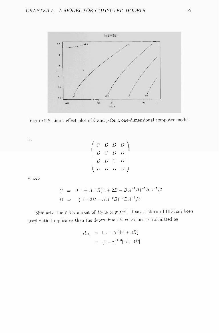
CHAPTER 5. A MODEL FOR COMPUTER MODELS
2 0 -
1 9
1-8 -
Q-
1.7 ^
1.6 -
1-5 -
In(EIVISE)
7A^/; -001 -005 01 -05 -1
thelal
Figure 5.5: Joint effect plot of 9 and p for a one-dimensional computer model.
as
wliere
/ C D D D \
D C D D
D D C D
D D D C \
C = A-'+A^'B{A + 2B-BA''B)''B.\--'/i
D = -{A + 2B - BA-'B)-'BA'^/3.
Similarly, the determinant of Rs is requhed. If sa\- a 50 run LHD had been
used with 4 replicates then the determinant is coiiA-enientlv calculated as
IKDI = \A-B\'\A + 3B\
T a 50 .4 + 351.

CHAPTER 5. A MODEL FOR COMPUTER MODELS 83
2 0 -
1 9 -
1 8
CM Q-
17 -
1.6 -
1.5 -
In(EMSE)
r 7/5 / Vs
001 ,005 -01 .05 -1
Ihetal
Figure 5.6: Joint effect plot of 9i and p2 for the model of computer models.
5.5 Some Apphcations of the Results
The model developed in the prcA-ious section used o" = 1. For other A-alues of a
the marginal effect of n^. for example, is gi\-en Iw-
In(EMSE) = log{a') - ^(622 + 6 5) - b^iP - bnin')'-
Figure 5.9 gives the results of Table 3.5. the predictions for the fitttnl c|uadratic
model giA-en in Table 5.6 with the i)arauieters as in Table 2.9, and the marginal
effect AA-ith cj2 = 123.556,
The agreement betAveen the results of Table 3.5 and the predictions from the
fitted quadratic model is quite good. On tiie other hand the marginal effect is
biased but also parallel to the pattern exhibited IJA- the data.
5.6 Conclusions
In this chapter an experiment on computer models has been conducted. This
(>xperiment Avas concerned \A-ith establishing a relationship between the Empirical
Mean Square Error and the parameters of a four dimensional computer model,
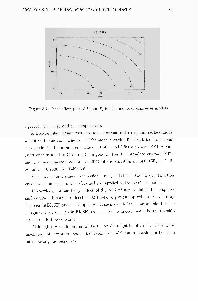
CHAPTER 5. A MODEL FOR COMPUTER MODELS s4
.1 -
-05 '
S -01 -
005 -
001
In(EMSE)
-?; :-.001 005 01 .05 .1
Ihelal
Figure 5.7; Joint effect plot of 9i and 2 for the model of computer models.
^ 1 , , . . , 6*4, P l , . . . , /J4 and the sample size n.
A Box-Behnken design was used and. a second order resjxjiise surface model
was fitted to the data. The form of the model AA-as simplified to take into account
s>-mmetries in the parameters. The (luaclratic model fitted to the ASET-B com
puter code studied in Chapter 3 is a good fit (residual standard error=0.2847),
and the model accounted for over 95'X of the xariation in In(EMSE) \\-ith R-
Squared = 0.9536 (see Table 5.6).
Expressions for the mean, main effects, marginal effects, tAA-o factor interaction
effects and joint effects Avere obtained and applied to the ASET-B model.
If knoAvledge of the likely values of 9.p and a^ are available, the response
surface model is shown, at least for ASET-B, to giA-e an approximate relationship
betAA-een In(EMSE) and t he sample size. If such knowledge is unaA-ailable then the
marginal effect of n on In(EMSE) can be used to approximate the relationship
up to an additiA^e constant.
Although the results are useful better results might be obtained b}- using the
inachinerA- of computer models to develop a model but smoothing rather than
interpolating the responses.
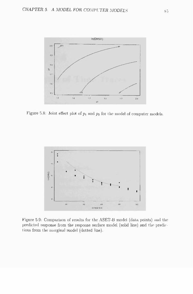
CHAPTER 5. A MODEL FOR COMPUTER MODELS N j
Figure 5.8: Joint effect plot of pi and p2 for the model of computer models.
Figure 5.9: Comparison of results for the ASET-B model (data points) and the predicted response from the response surface modef (solid hue) and the predictions from the marginal model (dotted line).
Chapter 6
Analysis of Time Traces
6.1 Introduction
Many computer models proA-icle a trace of responses at \-arious A-alues of a time
parameter. For example, the ASET-B program proA-ides the lunght of th(> smoke
layer at intervals of 5 seconds.
Although such time trace responses are A-er\- cominonl\- used, the literature
has focused on computer experiments Avith a uniA-ariat e response. In this chapter
consideration Avill be on hoAV a response as a function of time could be anah-scHl.
6.2 Possible Methods
When the data consists of a trace OAer time for the various input conditions a
number of \A-aA-s of aiiah-sing the data suggest Ihemseh-es:
1. Do a separate calculation for each time point. This Avould giA-e estimates of
9i.... ,9d and Pl Pfi for each A-afue of time that has been iiiA-cAstigatcnf.
Hence estimates of the response at each of the times can be generated using
the appropriate A-alues of the ^s and ps in the linear predictor. To gc>t
estimates of the response at intermediate times a cubic smoothing spline of
the predictions can be made.
86
CHAPTER 6. ANALYSIS OF TIME TRACES 87
2. Regard tim.e as an additional input parameter. This \A-ould give rise to tAvo
additional parameters 9d+i and p^+i describing the correlation as a fimc tion
of time. The data A-ector from an n - r u n Latin Hypercube design Avith T
times would be of length nT.
Both methods wiU be developed and apphed in turn to the ASET-B model.
The advantages and disadvantages of each method Avill be discussed.
Assuming that a time average gives a complete representation of the full en
semble in the second method described above, this SAsteni can be considered as
a special case of ergodic properties of particular interest Ergodicity.
E rgod ic i ty
Ergodicity is an attribute of a stochastic process. The foundation of the Markov
chain theory is tli(> ErgodicitA- Theorem. It establishes the conditions under Avhic h
a Markov chain can be anaJA-secl to determine its steadA' state behaviour. In
general it is a process that leads to the probabihty of a hmiting form that is
independent of the initial conditions. In the proposed second method aboA-e. sav
time as an additional input parameter, it is about the time average propert>- of
the process that carries an imphcit ergodicity [see Gray (1987), for more details].
It is common to assume ergodicity, where there is interchangeabilitA- of time
averages Avith the ensemble a,A-erage. In practical terms, this means measuring the
impulse responses at different times and then computing the time delaA- correla
tion function. In this scenario, cwafuation of ergodicitv as a feature of dynamic-
behaviour is important, not opposing the assumption facilitating the use of a
probabilitv model (Sposito, 1997). A paper bv Pribadi et al. (2001) on a reduc
tion method for Markov chains ])roved the importance of preserAung the propertA-
of ergodicit.A'. This approach is especiall}- useful in the area of simulation and
performance estimation.

CHAPTER 6. ANALYSIS OF TIME TRACES bb
6.2.1 Separate Calculation for a Number of Time Points
A 50 run LHD was generated. For each run the ASET-B program AA-as used to
generate the height of the smoke ta.A-er at 5 second interA-als up to 100 si^conds.
Figure 6.1 giA-es the generated traces. Table 6.1 and Table 6.2 giA-e the input
variables for the 50 run LHD. Table 6.3. Table 6.4, Table 6,5. Table 6.6, Table 6.7
and Table 6.8 giA-e the heights of the smoke laAcr at 5 second intervals up to 100
seconds for runs 1 to 50 of the same LHD.
c ~ ^ _
O _
Laye
r (F
t.)
8
Sm
oke
6 1
"b
CT} ^ —
X
CN - ,
O -
1 1
0 20
ASET-B Results
1 1
40 60
Time (sees)
1
80
1
100
Figure 6.1; Generated Time Tracc\s for the ASET-B Latin Hypercube Expcnin U>111
For each time period a separate computer model was fitted using th(> method
ology of Sacks et al (1989b), giving A-alues of 9 and p for each tiiii(> period.
Figure 6.2 and Figure 6.3 giA-e plots of the A-alues of 0 and p. The graphs show
that therc^ is considerable A-ariation in the 0 and p A-alues and that these \-a.lues
are not smooth.
For a Heat Loss Fraction of 0.85, Fire Height of 2.5 ft. Room Ceihng Height of
9 ft and Room Floor Area of 150 sq. ft, predictions of the smoke la\-er height at
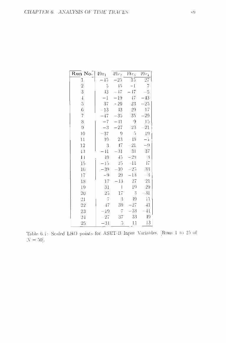
CHAPTER 6. ANALYSIS OF TIME TRACES s9
Run No. 1 2 3 4 5 6 7 8 9 10 11 12 13 14 15 16 17 18 19 20 21 22 23 24 25
49xi
-45 —5 43 -1 37
-13 -47 -7 -3 -37 19 3
-41 49
-15 -39 -9 17 31 25 7 47
-19 -27 -31
49.T2
-25 -45 -47 -19 -29 43
-35 -41 -27
9 23 47
-31 45 25
-39 29
-13 1 17 3 39 7 37 5
49.-T3
15 -1 -47 47
-23 29 35 9 23 5
-49 -21 31
^29 -11 -25 -13 27 19 3 49
-27 -33 33 11
49.r4
27 -7 -5 -43 -25 17
-29 -15 -21 19 -1 -9 37 3 47 33 -3 21 29
-31 11 41
-41 49 13
Table 6.1; Scaled LHD points for ASET-B Input Variables, [Runs 1 to 25 of A' = 50],
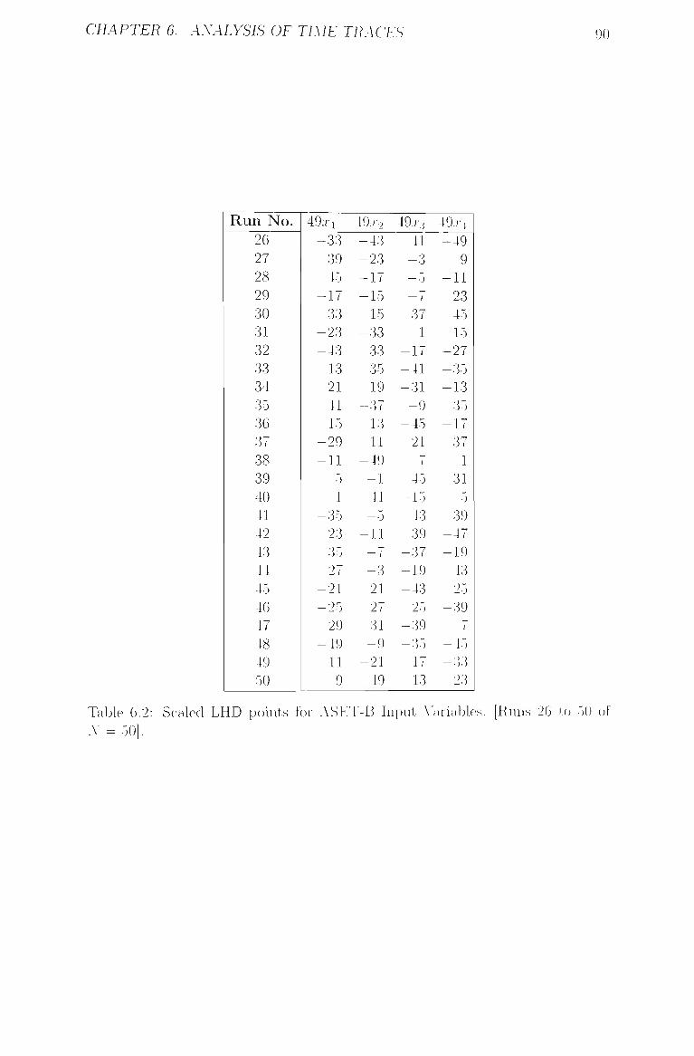
CHAPTER 6. ANALYSIS OF TIME TRACES 90
Run No. 26 27 28 29 30 31 32 33 34 35 36 37 38 39 40 41 42 43 44 45 46 47 48 49 50
49xi
-33 39 45
-17 33
-23 -43 13 21 41 15
-29 -11
5 1
-35 23 35 27
-21 -25 29
-49 11 9
49.r2
-43 -23 -17 -15 15
-33 33 35 19
-37 13 11
-49 -1 41 —5 -11 — 7
-3 21 27 31 -9 -21 49
49.r3
41 -3 —5 — /
37 1
-17 -41 -31 -9 -45 21 ('
45 -15 43 39
-37 -19 -43 25
-39 -35 17 13
49.r4 -49 9
-11 23 45 15
-27 -35 -13 35
-17 -37
1 31 5 39
-47 -19 43 25
-39 7
-45 -33 -23
Table 6.2: Scaled LHD points for ASET-B Input \ariables. [Runs 20 to 5f) of A' )0].
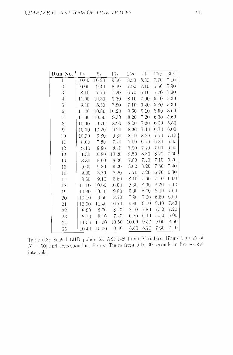
CHAPTER 6. ANALYSIS OF TIME TRACES 91
R u n N o . 1 2 3 4 5 6 7 8 9 10 11 12 13 14 15 16 17 18 19 20 21 22 23 24 25
O.s 10.60 10.00
8.10 11.90 9.10
11.20 11,40 10.40 10.90 10.20
8.00 9.10
11,30 8.80 9.60 9.00 9.50
11.10 10.80 10.10 12.00 8.90 8.70
11.30 10.40
5.S 10.20 9.40 7.70
10,80 8,50
10,80 10.50 9.70
10.20 9.80 7.80 8.80
10.80 8.60 9.30 8.70 9.10
10.60 10.40
9.50 11.40
8.70 8,10
11,00 10,00
lO.s 9.60 8.60 7.20 9.30 7.80
10.20 9.30 8.90 9.20 9.30 7.40 8.40
10.20 8.20 9.00 8,20 8.60
10.00 9.80 8.70
10.70 8.40 7.40
10.50 9.40
los 8.90 7.90 6.70 8.10 7.10 9.60 8.20 8.00 8.30 8.70 7.00 7.90 9.50 7.80 8.60 7,70 8.10 9.30 9.30 7.90 9.90 8.10 6.70
10.00 8.80
20.s 8.30 7.10 6.10 7.00 6.40 9.10 7.20 7.20 7.40 8.20 6.70 7.40 8.80 7.40 8.20 7.20 7.60 8.60 8.70 7.20 9.10 7.80 6.10 9.50 8.20
25s 7.70 6.50 5.70 6.10 5.80 8.50 6.30 6.50 6.70 7.70 6.30 7.00 8.20 7.10 7.80 6.70 7.10 8.00 8.10 6.60 8.40 7.50 5.50 9.00 7.60
30.S 7.10 5.90 5.20 5.30 5.30 8.00 5.60 5.80 6.00 7.10 6.00 6.60 7.60 6.70 7.40 6.30 6.60 7.40 7.60 6.00 7.80 7.20 5.00 8.50 7.10
Table 6.3: Scaled LHD points for ASET-B Input Variables. [Runs 1 to 25 of A' = 50] and corresponding Egress Times from 0 to 30 seconds in Hve second intervals.
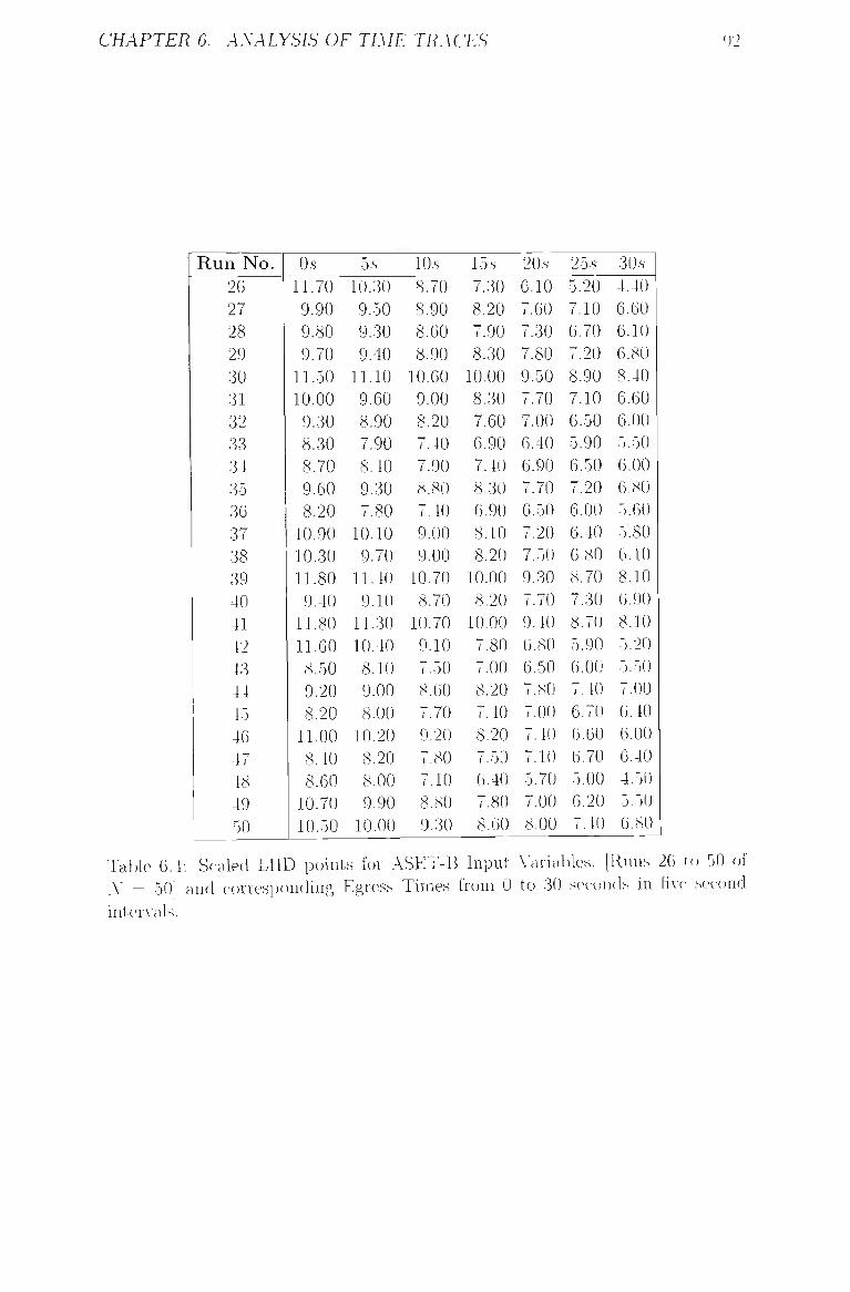
CHAPTER 6. ANALYSIS OF TIME TRACES 92
Run No. 26 27 28 29 30 31 32 33 34 35 36 37 38 39 40 41 42 43 44 45 46 47 48 49 50
Os 11.70
9.90
9.80
9.70
11.50
10.00
9.30
8.30
8.70
9.60
8.20
10.90
10.30
11.80
9.40
11.80
11.60
8.50
9.20
8.20
11.00
8.40
8.60
10.70
10.50
5 s
10.30
9.50
9.30
9.40
11.10
9.60
8.90
7.90
8-40
9.30
7.80
10.10
9.70
11.40
9.10
11.30
10.40
8.10
9.00
8.00
10.20
8.20
8.00
9.90
10.00
10s 8.70
8.90
8.60
8.90
10.60
9.00
8.20
7.40
7.90
8.80
7.40
9.00
9.00
10.70
8.70
10.70
9.10
7.50
8.60
7.70
9.20
7.80
7.10
8.80
9.30
15s 7.30
8.20
7.90
8.30
10.00
8.30
7.60
6.90
7.40
8.30
6.90
8.10
8.20
10.00
8.20
10.00
7.80
7.00
8.20
7.40
8.20
7.50
6.40
7.80
8.60
20s 6.10
7.60
7.30
7.80
9.50
7.70
7.00
6.40
6.90
7.70
6.50
7.20
7.50
9.30
7.70
9.40
6.80
6.50
7.80
7.00
7.40
7.10
5.70
7.00
8.00
25s 5.20
7.10
6.70
7.20
8.90
7.10
6.50
5.90
6.50
7.20
6.00
6.40
6.80
8.70
7.30
8.70
5.90
6.00
7.40
6.70
6.60
6.70
5.00
6.20
7.40
30s 4.40
6.60
6.10
6.80
8.40
6.60
6.00
5.50
6.00
6.80
5.60
5.80
6.10
8.10
6.90
8.10
5.20
5.50
7.00
6.40
6.00
6.40
4.50
5.50
6.80
Table 6.4: Scaled LHD points for ASET-B Input Variables, [Runs 26 to 50 of A' = 50] and corresponding Egress Times from 0 to 30 seconds in fiA-e second intervals.
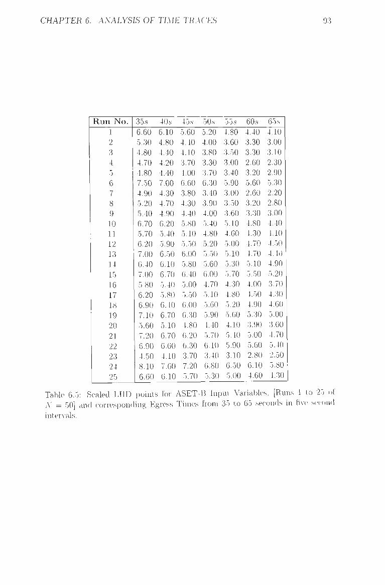
CHAPTER 6. ANALYSIS OF TIME TRACES 93
Run No. 1 2 3 4 5 6 7 8 9 10 11 12 13 14 15 16 17 18 19 20 21 22 23 24 25
35s 6.60
5.30
4.80
4.70
4.80
7.50
4.90
5.20
5.40
6.70
5.70
6.20
7.00
6.40
7.00
5.80
6.20
6.90
7.10
5.60
7.20
6.90
4.50
8.10
6.60
40s 6.10
4.80
4.40
4.20
4.40
7.00
4.30
4.70
4.90
6.20
5.40
5.90
6.50
6.10
6.70
5.40
5.80
6.40
6.70
5.10
6.70
6.60
4.10
7.60
6.10
45s 5.60
4.40
4.10
3.70
4.00
6.60
3.80
4.30
4.40
5.80
5.10
5.50
6.00
5.80
6.40
5.00
5.50
6.00
6.30
4.80
6.20
6.30
3.70
7.20
5.70
50s 5.20
4.00
3.80
3.30
3.70
6.30
3.40
3.90
4.00
5.40
4.80
5.20
5.50
5.60
6.00
4.70
5.10
5.60
5.90
4.40
5.70
6.10
3.40
6.80
5.30
55s 4.80
3.60
3.50
3.00
3.40
5.90
3.00
3.50
3.60
5.10
4.60
5.00
5.10
5.30
5.70
4.30
4.80
5.20
5.60
4.10
5.40
5.90
3.10
6.50
5.00
60s 4.40
3.30
3.30
2.60
3.20
5.60
2.60
3.20
3.30
4.80
4.30
4.70
4.70
5.10
5.50
4.00
4.50
4.90
5.30
3.90
5.00
5.60
2.80
6.10
4.60
65s 4.10
3.00
3.10
2.30
2.90
5.30
2.20
2.80
3.00
4.40
4.10
4.50
4.40
4.90
5.20
3.70
4.30
4.60
5.00
3.60
4.70
5.40
2.50
5.80
4..30
Table 6.5: Scaled LHD points for ASET-B Input Variables, [Runs 1 to 25 of X = 50] and corresponding Egress Times from 35 to 65 seconds in fiA-e second intervals.

CHAPTER 6. ANALYSIS OF TIME TRACES 94
Run No. 26 27 28 29 30 31 32 33 34 35 36 37 38 39 40 41 42 43 44 45 40 47 48 49 50
35s 3.80
6.10
5.60
6.30
7.90
6.00
5.50
5.20
5.70
6.30
5.30
5.20
5.60
7.50
6.50
7.60
4.60
5.10
6.60
6.00
5.40
6.10
4.00
5.00
6.40
40s 3.20
5.70
5.20
5.90
7.50
5.60
5.10
4.80
5.30
5.90
4.90
4.70
5.10
7.00
6.20
7.10
4.20
4.80
6.30
5.70
4.90
5.80
3.50
4.50
5.90
45s 2.70
5.30
4.80
5.50
7.10
5.10
4.70
4.50
5.00
5.50
4.60
4.30
4.60
6.60
5.80
6.60
3.80
4.40
5.90
5.40
4.50
5.50
3.10
4.10
5.60
50s 2.30
4.90
4.50
5.10
6.70
4.70
4.30
4.20
4.70
5.20
4.30
3.90
4.20
6.10
5.50
6.10
3.40
4.10
5.60
5.20
4,10
5.20
2.70
3,70
5.20
55 s
1.90
4.60
4.20
4.80
6.30
4.40
4.00
4.00
4.40
4.90
4.10
3.50
3.80
5.80
5.20
5.70
3.10
3.90
5.30
4.90
3.80
5.00
2.40
3,30
4.90
60s 1.50
4.30
3.90
4.40
6.00
4.00
3.70
3.70
4.20
4.60
3.80
3.20
3.50
5.40
5.00
5.30
2.80
3.60
5.10
4.60
3.40
4.80
2.00
3.00
4.60
65s 1.20
4.00
3.70
4.10
5.70
3.70
3.30
3.50
4.00
4.30
3.60
2.80
3.20
5.10
4.70
5.00
2.60
3.40
4.80
4.40
3.10
4.60
1.60
2.80
4.40
Table 6.6; Scaled LHD points for ASET-B Input Variables. [Runs 20 to 50 of A' = 50] and corresponding Egress Times from 35 to 65 seconds in fiA-e second inter\-als.
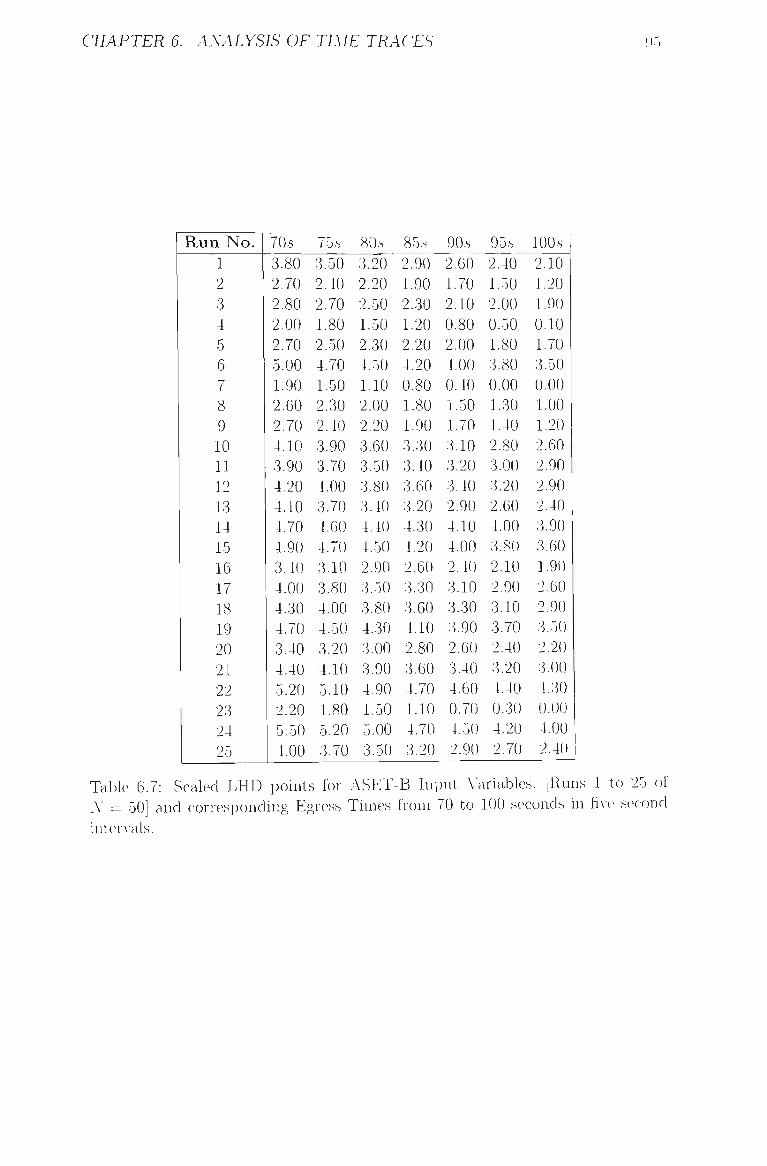
CHAPTER 6. ANALYSIS OF TIME TRACES
Run No. 1 2 3 4 5 6 7 8 9 10 11 12 13 14 15 16 17 18 19 20 21 22 23 24 25
70s 3.80
2.70
2.80
2.00
2.70
5.00
1.90
2.60
2.70
4.10
3.90
4.20
4.10
4.70
4.90
3.40
4.00
4.30
4.70
3.40
4.40
5.20
2.20
5.50
4.00
75 s
3.50
2.40
2.70
1.80
2.50
4.70
1.50
2.30
2.40
3.90
3.70
4.00
3.70
4.00
4.70
3.10
3.80
4.00
4.50
3.20
4.10
5.10
1.80
5.20
3.70
80s 3.20
2.20
2.50
1.50
2.30
4.50
1.10
2.00
2.20
3.60
3.50
3.80
3.40
4.40
4.50
2.90
3.50
3.80
4.30
3.00
3.90
4.90
1.50
5.00
3.50
85s 2.90
1.90
2.30
1.20
2.20
4.20
0.80
1.80
1.90
3.30
3.40
3.60
3.20
4.30
4.20
2.60
3.30
3.60
4.10
2.80
3.60
4.70
1.10
4.70
3.20
90s 2.60
1.70
2.10
0.80
2.00
4.00
0.40
1.50
1.70
3.10
3.20
3.40
2.90
4.10
4.00
2.40
3.10
3.30
3.90
2.60
3.40
4.60
0.70
4.50
2.90
95s 2.40
1.50
2.00
0.50
1.80
3.80
0.00
1.30
1.40
2.80
3.00
3.20
2.60
4.00
3.80
2.10
2.90
3.10
3.70
2.40
3.20
4.40
0.30
4.20
2.70
100s
2.10
1.20
1.90
0.10
1.70
3.50
0.00
1.00
1.20
2.60
2.90
2.90
2.40
3.90
3.60
1.90
2.60
2.90
3.50
2.20
3.00
4.30
0.00
4.00
2.40
Table 6.7: Scaled LHD points for ASET-B Input Variables. [Runs 1 to 25 of A = 50] and corresponding Egress Times from 70 to 100 seconds in fi\-e second inter \-als.
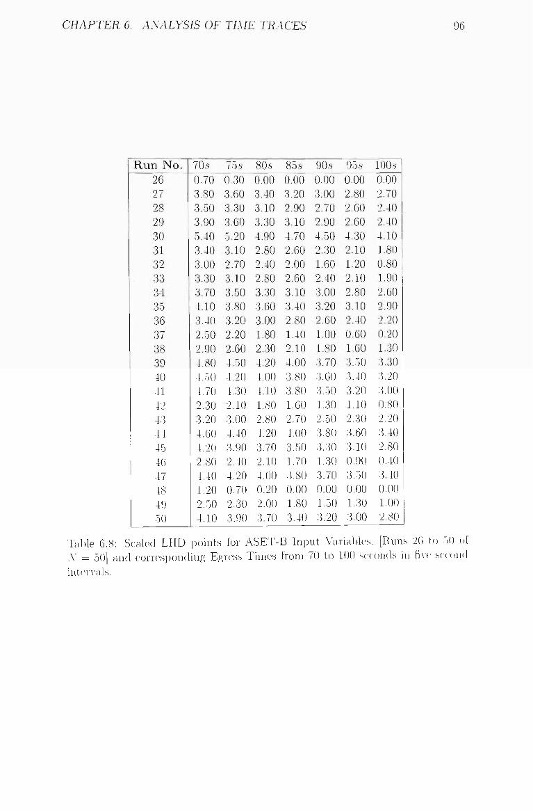
CHAPTER 6. ANALYSIS OF TIME TRACES 96
Run No. 26 27 28 29 30 31 32 33 34 35 36 37 38 39 40 41 42 43 44 45 46 47 48 49 50
70s 0.70
3.80
3.50
3.90
5.40
3.40
3.00
3.30
3.70
4.10
3.40
2.50
2.90
4.80
4.50
4.70
2.30
3.20
4.60
4.20
2.80
4.40
1.20
2.50
4.10
75s 0.30
3.60
3.30
3.60
5.20
3.10
2.70
3.10
3.50
3.80
3.20
2.20
2.60
4.50
4.20
4.30
2.10
3.00
4.40
3.90
2.40
4.20
0.70
2.30
3.90
80s 0.00
3.40
3.10
3.30
4.90
2.80
2.40
2.80
3.30
3.60
3.00
1.80
2.30
4.20
4.00
4.10
1.80
2.80
4.20
3.70
2.10
4.00
0.20
2.00
3.70
85s 0.00
3.20
2.90
3.10
4.70
2.60
2.00
2.60
3.10
3.40
2.80
1.40
2.10
4.00
3.80
3.80
1.60
2.70
4.00
3.50
1.70
3.80
0.00
1.80
3.40
90s 0.00
3.00
2.70
2.90
4.50
2.30
1.60
2.40
3.00
3.20
2.60
1.00
1.80
3.70
3.60
3.50
1.30
2.50
3.80
3.30
1.30
3.70
0.00
1.50
3.20
95s 0.00
2.80
2.60
2.60
4.30
2.10
1.20
2.10
2.80
3.10
2.40
0.60
1.60
3.5t)
3.40
3.20
1.10
2.30
3.60
3.10
0.90
3.50
0.00
1.30
3.00
100s
0.00
2.70
2.40
2.40
4.10
1.80
0.80
1.90
2.60
2.90
2.20
0.20
1.30
3.30
3.20
3.00
0.80
2.20
3.40
2.80
0.40
3.40
0.00
1.00
2.80
Table 6.8; Scaled LHD points for ASET-B Input Variables, [Runs 20 to 50 of A' = 50] and corresponding Egress Times from 70 to 100 seconds in fi\-e second iuter\-a,ls.
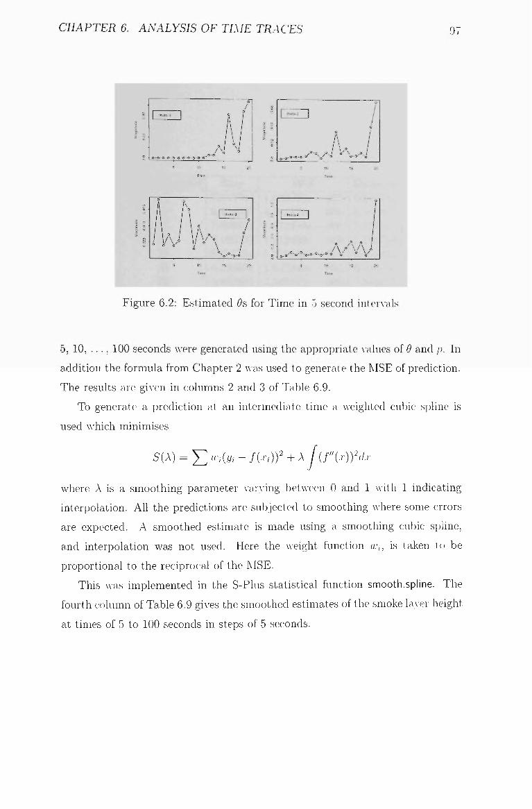
CHAPTER 6. ANALYSIS OF TIME TRACES 97
o
/ 1 ' - - 1 ; /
.o.N^ °
0
1A J •3 o o
0
\
1 A'" I h , . ,
o
\ o
' 1 0
/ 0
/ 3-0
10 15
o
/ 1.,.-. 1 /
15 20
1 1.. . . 1
Figure 6.2: Estimated ^s for Time in 5 second interval
5, 10, . . . , 100 seconds were generated using the appropriate \-alues of 9 and p. In
addition the formula from Chapter 2 was used to generate the MSE of prediction.
The results are giA-en in columns 2 and 3 of Table 6.9.
To generate a prediction at an intermediate time a Aveighted cubic spline is
used which minimises
S{X) = '£w,{y,-f{.r,))' + xl{r{.r)Ydx
where A is a smoothing parameter A-arA'ing betAveen 0 and 1 \\-itli 1 indicating
interpolation. All the predictions are subjected to smoothing where some errors
are expected. A smoothed estimate is made using a smoothing cubic spline,
and interpolation was not used. Here the Aveight function w,, is taken to be
proportional to the reciprocal of the MSE.
This Avas implemented in the S-Plus statistical function smooth.spline. The
fourth column of Table 6.9 giA-es the smoothed estimates of the smoke laA-er height
at times of 5 to 100 seconds in steps of 5 seconds.
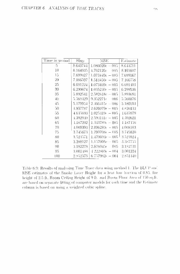
CHAPTER 6. ANALYSIS OF TIME TRACES 9,s
Time in second
5 10 15 20 25 30 35 40 45 50 55 60 65 70 75 80 85 90 95 100
Blup
8.643744
8.164935
7.699427
7.166597
6.691224
6.299874
5.892541
5.569429
5.179954
4.937787
4.635693
4.392940
4.187202
4.009393
3.745673
3.523571
3.388127
3.182278
3.001488
2.852575
MSE 1.086020e -
4.762126e -
1.073449e -
1.513450e -
1.073449c -
1.035240f -
2.582818e -
9.352271f -
2.466415c -
2.626079e -
1.025419c -
2.594141c -
1.343789c -
2.896289c -
1.790708e -
1.470694e -
1.157005e-
2.876045c -
4.222809c -
6.757982e -
- 005
-005
-005
-005
-005
-005
-005
-006
-006
-005
-005
-005
-005
-005
-005
-005
-005
-005
-004
-004
Estimate
8.043711
8.165607
7.699167
7.166758
6.691403
6.299536
5.893691
5.568876
5.180113
4.836133
4.635979
4.392621
4.187450
4.008583
3.745820
3.523924
3.3S7755
3.182731
3.001324
2.851340
Table 6.9: Results of analysing Time Trace data using method 1. The BLfT' and
MSE estimates of the Smoke Layer Height for a heat lo,ss fraction of 0.85. fire
lunght of 2.5 ft. Room Ceihng Height of 9 ft. and Room Floor Area of 150 sq.ft.
are based on separate fitting of computer models for each time and the Estimate
column is based on using a \\-eighted cubic spline.
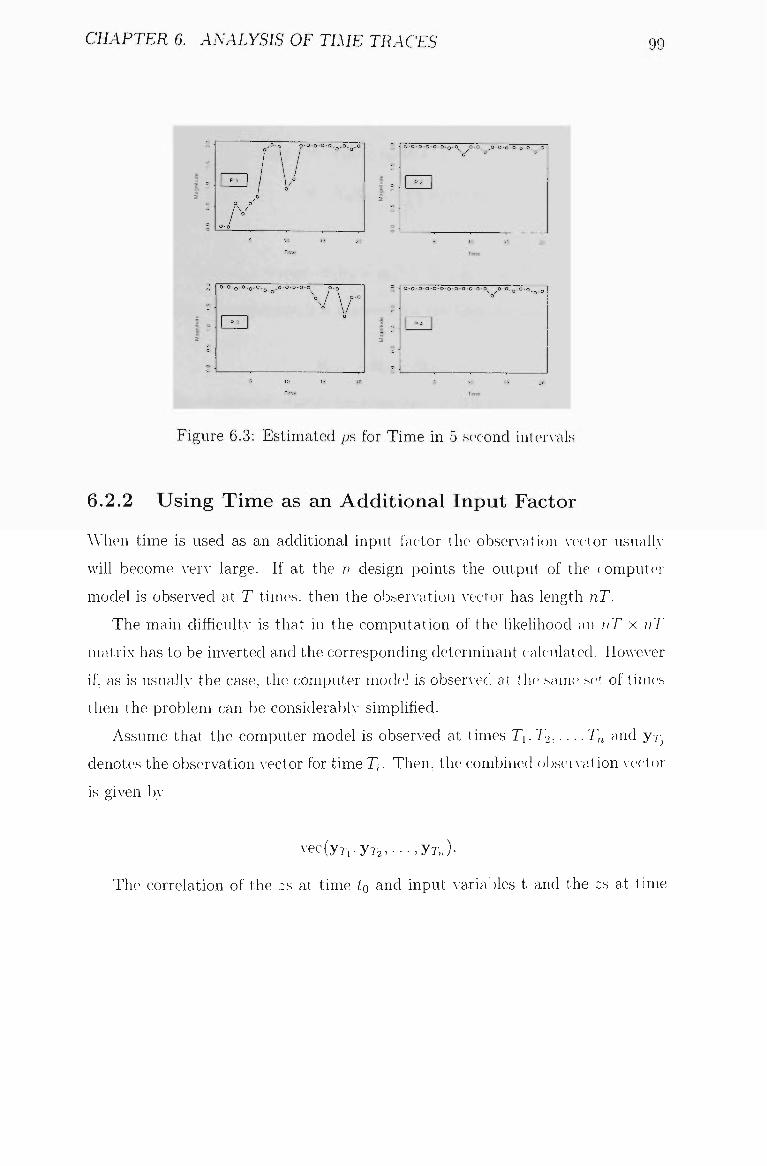
CHAPTER 6. ANALYSIS OF TIME TRACES 99
s
2
O-o o-o-o-o-o.„,o, ,o O , / 0 o
1" 1 I,. / ° 0
o o^
/ ° o-o
5 10 15 20
0-0-f,,0.-,.0,_ ,0-0-0-0-0 o-o
o / \ o-o
1 P3 1
5 10 15 20
s
=
O-O-O-O-O-O-o-O 0-0 O-O-O-O-o-O 0
1 - 1
5 10 15 20
1 ^ 1
5 10 IS 20
Figure 6.3: Estimated ps for Time in 5 second interAals
6.2.2 Using Time as an Additional Input Factor
When time is used as an additional input factor the obserA-ation \-(xtor usuallA-
Avill become A-ery large. If at the n design points the output of the computer
model is observed at T tiinc\s. then the obserA-ation A-ector has length nT.
The main difficulty is that m the computation of the likelihood an riT x iiT
matrix has to be im^erted and the corresponding determinant calculated. HoAA-cA-er
if, as is usually the case, the computer model is obserA-cxl at the same s(>t of times
then the problem can be considerably simplified.
Assume that the computer model is observed at times Ti.Tz... • .Tn and yj- .
denotes the obserA-ation vector for time T,. Then, the combined observation A-ector
is dA-en Iw
vec(yri.yr2,---,y7;,)-
The correlation of t he ^s at time io and input A-arial-)les t and the zs at t ime

CHAPTER 6. ANALYSIS OF TIME TRACES 100
uo and input variables u is (lc>noted bA-
R D T = 7?o(^o-"n)R(t.u) d
= Ro{tn,UQ)Y\Rk{tk-J'k) k=i
Avhere
Rk{tk, Uk) = exp{-9k\tk - Uk\'"') 0 < pfc < 2; ^^ > 0.
In this notation the subscript 0 is reserved for the time variable.
Now
RDT = R r X' RD
where Ry, the correlation matrix for responses at different times for a fixed set
of conditions, is given by
R^[^.y] = exp(-^o|T, - T^f") /..; = 1 T
and R D , the correlation matrix for the responses at tlu^ design points at a fixed
time, is given Iw-
fc=l
When calculating the likelihood the folloAAung properties of the Kronecker product
and
I RDT I = |Rrl |RD|
can be used to simplifA- the calculations. Using these properties, means that onh-
matric-es of size T xT and n x n rather than nT x tiT ha\-e to be dealt with.
When predicting at x^ = (x, T)-^ Ave use
y = 3 + vlr(^R^{y-lft)
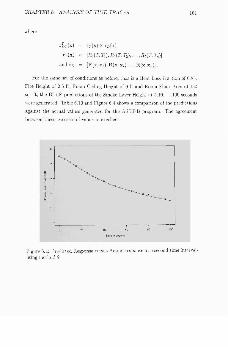
CHAPTER 6. ANALYSIS OF TIME TRACES 101
A\-here
r L r W = r r ( x ) g r D ( x )
rr(x) = [i?o(r.ri),i?„(r.r2),....i?o(r,r„)]
and TD = [R(x, xi) , R(x, X2) . . . , R(x. x„)] .
For the same set of conditions as before, that is a Heat Loss Fraction of 0.85.
Fhe Height of 2.5 ft. Room Ceiling Height of 9 ft and Room Floor Area of 150
sq. ft, the BLUP predictions of the Smoke LaA-er Height at 5.10, 100 seconds
were generated. Table 6.10 and Figure 6.4 shoAvs a comparison of the predictions
against the actual values generated for the ASET-B program. The agreement
between these two sets of values is excellent.
Figure 6.4: Predicted Response \-ersus Actual response at 5 second time inter\-als
usinK method 2.

CHAPTER 6. ANALYSIS OF TIME TRACES 102
Time (s)
0 5 10 15 20 25 30 35 40 45 50 55 60 65 70 75 80 85 90 95 100
Actual
9.00
8.65
8.17
7.67
7.18
6.73
6.31
5.92
5.57
5.25
4.97
4.70
4.46
4.23
4.03
3.83
3.05
3.48
3.31
3.15
2.99
Predicted
8.9822
8.6573
8.1520
7.6683
7.1782
6.7045
6.2632
5.9105
5.5409
5.1862
4.8869
4.6490
4.4030
4.2256
3.9398
3.7335
3.5657
3.3510
3.2570
3.0699
2.8689
Table 6.10: Predicted Response versus Actual response at fiA-e second time iiiter-\-als using method 2.
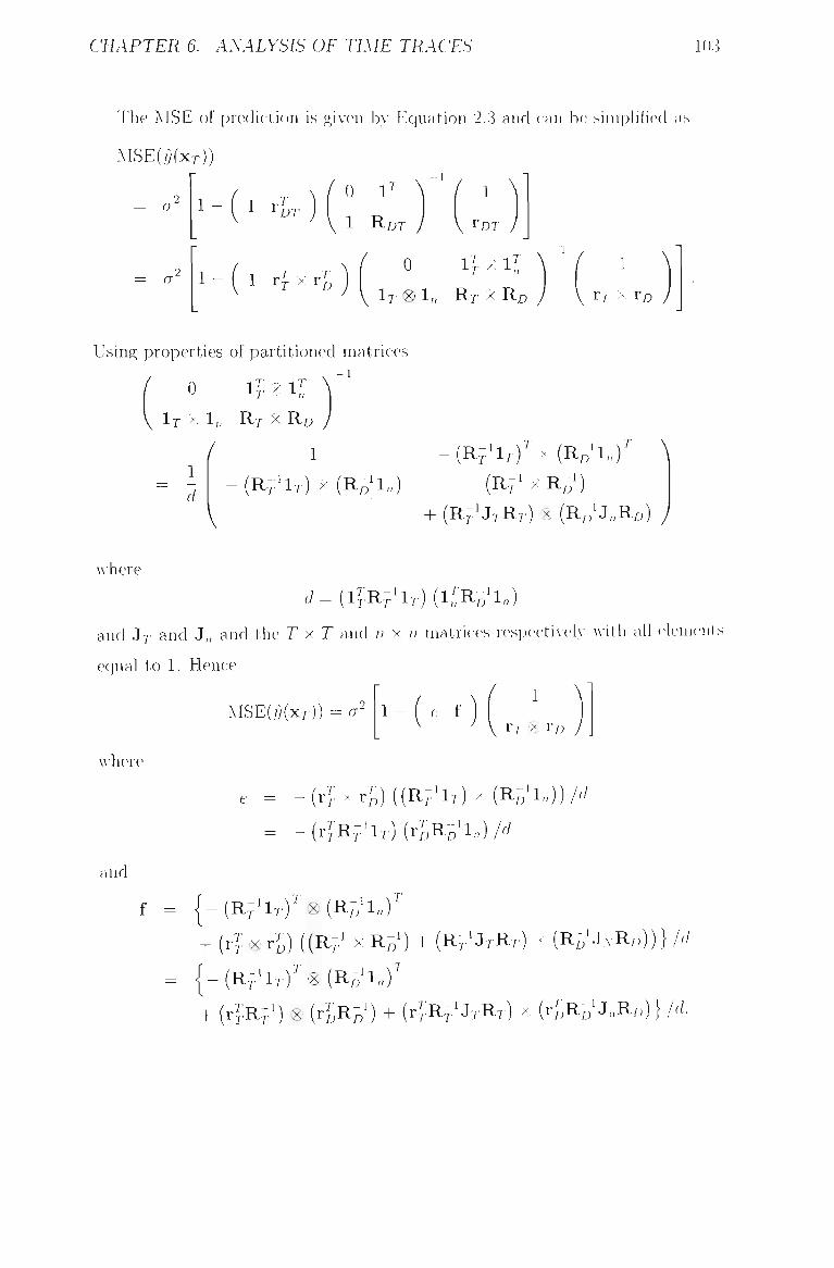
CHAPTER 6. ANALYSIS OF TIME TRACES 103
The MSE of prediction is given by Equation 2.3 and can be simplified as
MSE(y(xr))
1 a 1 - ( 1 vl^
0 1^
1 R D T
= a 1 - ( 1 rl % r f L J, ^, 1 D
0 I f R 1^
I T ® In R T X RD
1
r r X XD
Using properties of partitioned matrices
0 1 ? « 1 ^
1 T ' X 1 „ R T ' X ' R D
1 / 1 - ( R ^ ' l T ) ^ x ( R D l n ) ^ \
- ( R ^ i l r ) x ( R B ' l . ) ( R T ' X R Z ; )
\^ + ( R ^ I J T R T ) X ( R D ' J . R D ) )
AA'here
d={\lRf'\T){^l'^-D^n)
and J r and J„ and the T x T and n x n matrices respectiA-el.A- \A-ith all elements
ecjual to 1. Hence
1
r , X rD MSE(y(xr)) = o"' 1 - e f
\\-here
and
e = - ( r ? x r a ( ( R ^ 4 T ) x ( R B ^ l , 0 ) A /
= - ( r ? R ^ 4 T ) ( r S R B ^ l . ) / r f
f = | _ ( R - i l r ) ' ^ « ( R B ' l n ) ^
+ ifr^rl) {{R-^' X R D ' ) + ( R ^ ^ J T R T ) X ( R ^ M . V R D ) ) } / ^ /
= { - ( R ^ ^ l r ) ' ^ X ( R D ' l n ) ' ^
-f ifr^f) % ( r^RD ) + (r^RT^ J T R T ) « K R D J - R D ) } /d.
CHAPTER 6. ANALYSIS OF TIME TRACES 104
Therefore
^ SE(y(xT)) ^ . ^ { i - ^ ^ ^ ^ ^ , , ^ - ^ ^
+ (l^RT^r^) (inRB^rD) - (r^R^^rr) (r^R^'ro)
- (r^R^iJrRTrr) (r^RD^J^RD^rD)] j .
6.3 Conclusion
Many computer experiments give as a response a trace over time. TAVO different
methods for analysing such time traces haAe been presented.
In the first method each time set is analysed separatelA-, and an individual
model is estimated for each time point. To obtain predictions for untried inputs,
individual predictions at the experimental times are made using the models and
then a smoothed estimate is made using a smoothing cubic spline. When fitting
the sphne the reciprocal of the MSEs of the predictions are used as weights. In
the example this method appears to Avork well.
An alternatiA-e method uses time as an additional input lac tor. The apparent
clisadA-antage of the much increased dimension of the obserA-ation vector can. at
least for the product correlation famih- considered here, be OA-ercome !)>- using
Kronecker products in the calculation of the likelihood. One adA-antage of thc>
second method is that the usual formula for the MSE of prediction can be used.
Note that the second method assumes that the outputs at each time can be
modelled as realisations of stochastic processes with the same A-ariance-cc-)A-ariance
matrix, Avhile Avith the first method the variance-coA-ariance matrices are free to
var>-. If this homogeneity assumption is appropriate then the second metliod gives
a unified method AA-hich is easih- implemented.
Chapter 7
Discussion
7.1 Introduction
In previous chapters a number of im^estigations have been done on Computer Ex
periments. These investigations haA-e largely been dcAoted to practical ciuestions
such as how to best estimate para-met(>rs. how to summarise results, \\-hat sample
size should be used, what augmenting runs need to l)e added and how can time
trace responses be anal>-sc>d easily.
In Chaptc^r 2 the machinery of Computer Exijeriments was used to dcA-elop
a surrogate model for the ASET-B computer model. It AA-as shown hoAv a good
model giving ver>- accurate results could be generated from 50 runs of the ASET-
B program. Explicit expressions for the mean, main effects and tAA-o-factor in
teractions effec-ts Avere used to summarise the results Avhicli shoAvecl that the
non-additivitA- in this C'ase was quite small. These results wc>re conformed us
ing Functional AnalA-sis of Variance.
In Chapter 3 four different computer models AA-ere studied. For each model,
Latin Hypercube of 10, 20, . . ., 100 runs were produced and the four computer
models \\-cn e run at inputs corresponding to the design. For each sample size
the computer models were modelled as realisations of stochastic processes and
the abilit\- to predict at untried inputs AA-as assessed using ERMSE. AnalA-ses of
105

CHAPTER 7. DISCUSSION 106
the data shoAved that the computer models gave an approximate linear relation
ship betAA-een ERMSE'^^-^'' and n. HoAvcA-er. it was found that the slope of this
relationship varied considerably from model to model due to limited usefulness.
In Chapter 4 an expression for the prediction coAariance AA-as found, generating
the well knoAvn expression for the prediction A-ariance on MSE. For adding one
point at a time choosing the point from a candidate set Avith the maximum
prediction variance appears to work Aveh for the ASET-B model. For adding
more than one point at a time the points Avith the maximum determinant of the
prediction variance-covariance matrix AAcre selected.
In Chapter 5 Computer Experiments were studied. For a four dimensional
model realisations of a stochastic process Avith different A-alues of 0 and p chosen
using a Box-Behken response surface design Avere generated and the In(EMSE)
Avas modelled using a quadratic response surface. The relationship shows hoAv the
prediction variance depends on 0. p and n on aA-erage and the range of A-alues that
can be expected. Main effects and joint effect diagrams SIIOAV th(> effect of th(^
parameters and the interaction betAveen them. The results are shoAvn to match
those of Chapter 3 reasonal)fA- AA-ell.
In Chapter 6 tAvo methods of anah-sing Computer Experiments AA-hich give a
trace of responses OA-er time AAere studied and contrasted. One method iuA-oh-ed
fitting a separate model for each time studied. ,A.t an untried input, predictions
for each time point are produced using the separate^ modefs. For predicting at
an intermediate time, the predictions are combined using a Aveighted smoothing
sphne, Avith the weights iuA-ersely proportional to the MSEs of the predictions for
each time point.
The other method iiwoh^es adding time as an additional input factor. This
approach usualfA- giA-es a much larger dimensional observation A-ector leading to
problems in computing the likelihood. This can be overcome Iw- using the prop
erties of Kronecker products, reducing the problem to much more manageable
proportions. LIoAvever, using this method relies on a stronger assumption than
the first method. If this assumption is appropriate then straightforA\-ard predic
tions and estimates of the size of the prediction errors can be computed.

CHAPTER 7. DISCUSSION IO7
7.2 Limitations
7.2.1 Use of Latin Hypercube
While LHDs are available for aU sample sizes there are other designs that nia.A-
give superior results, certainly for more complex models. Some of the resiUts
found for sample sizes Avill probably giAC lower bounds on the performance of
these other designs.
7.2.2 Relationship between Sample Sizes and EMSE
Although an approximate linear relationship has been established betAveen
ERMSE" • and n this relationship is not optimal for aU computer models.
HoAveA er, as a compromise it appears to AA-ork reasonal)lA- AA-CII at least for the
fom computer models considered. Obviously, t his compromise maA- not apph' for
all computer models. EA-CU if it did. one remark that hmits its a])i)licabilitA- is
that the slope is different depending on the computer model.
7.2.3 Use of only Gaussian Product Correlation Structure
In this thesis OUIA- the Gaussian product correlation structure has f een used.
Other correlation structures may giA-e quite different results. The Gaussian c'or-
relation structure is infiniteh- mean scjuare differentiable for p = 2 and not mean
square differentiable for p 7 2. Correlation structures that giA-e intermediate
IcA-els of mean square clifferentiabilitA' nun- require different sample sizes.
7.3 Future Work
A number of extensions of the Avork conducted in this thesis suggest themselves:
7.3.1 Application to other Designs
Tlic^ \A-ork on sample sizes giA-en m Chapter 3 has been limited to Latin HA-percub(>
designs. Similar work should be conducted using other tA-pes of designs sue h as.
CHAPTER 7. DISCUSSION lOS
random orthogonal arrays. IMSE optimal Latin hypercubes. maximin Latin hy-
perculjes. orthogonal-array based Latin liA-percubes. uniform designs, orthogonal
Latin hypercubes. Hammersley sequence designs and other designs dcA-eloped for
Computer Experiments. It Avould be A-erA- interesting to see hoAv the relationship
betAveen ERMSE and n depends on the tA-pes of design. The same apphes \o the
work in Chapter 5.
On the other hand the augmenting methods examined and the methods de
veloped for the analysis of time traces are apphcable irrespectiA-e of the design
used.
7.3.2 Application to other Computer Models
The AA-ork on sample sizes Avas limited to four computer models. Further work of
this type would be useful for other computer models of A arA-ing dimensions and
complexitA-. EA'CII for farge scale computer models the amount of computing could
be reduced. For example, if a surrogate model based on 50 runs of the actiial
code was developed, then tli(> surrogate model could be used to se(> AA-hat would
haA-e been the effect of a different sample size on the aA-(n'agc> prediction error as
measured In- the ERMSE. These simulation studies AA-ould assist experinic>nters
in designing further experiments on the same code but also future experiments
on different code.
7.3.3 Prior Estimates of 0 and p
Fitting the model hv maximum likelihood is made much easier ])y good starting
A-alues of the 0 and p parameters. In the absence of good starting A-alues. random
starts can be used. Methods of determining good starting A-alues Avould be A-er\-
useful.
Prior to collecting the data it would also be useful to ha\-e an idea of likel\-
rangers for the 9 and ]; A-alues, in order to assist the determination of an appropriate
sample size. Methods for doing this Avould be of great benefit to experimenters.

CHAPTER 7. DISCUSSION 109
7.3.4 Model Diagnostics for Time Trace Data
TAVO methods of analysing time trace data from computer experiments AA-ere giA-en
in Chapter 0. The method based on the use of Kronecker products assumes much
more about the covariance matrix than does the other method. Diagnostics to see
whether this is a reasonable assumption need to be deA-eloped, More generallA-.
diagnostics tests and graphs for the correlation structure Avould be useful.
7.3.5 Multivariate Responses
Most Computer Experiments give as outputs more than one response Avhile the
results in Chapter 6 show hoAV time trace data can be convenienth- analAsed. It
would be useful to examine the benefits of analysing more than one response at
a time.

Bibliography
ARCHER, G.E.B., SALTELLI, A., and SOBOL. I.^l. (1997). ••Sensitivitv mea
surers. ANOVA-hke techniques and the use of bootstrap". .Journal of Stati.stical
Computation and Simulation, 58, 99 120.
BARTELL, S.M., GARDNER, R.H., ONEILL. R.V.. and GIDDINGS, J.M.
(1983). "Error analysis of predicted fate of anthracene in a simulated pond".
Environmental Toxicology and Chemistry. 2. 19 28.
BARTELL, S.M., LANDRUM, J.P.. GIESY, J.P.. and LEXTRSEE. G.J. (1981).
"'Simulated transport of polycyclic aromatic hydrocarbons in artificial streams".
In W.J. Mitch, R.W. Bosserman. and J.M. Klopatek. editors. Energy and Eco
logical Modelling, 133 143. Elsevier. NCAV York.
BATES. R.A., BUCK. R.J., RICCOMAGNO, E. and WYNN. H.P. (1996). •
Experimental Design and ObserA-ation for Large S\-steiiis". Jotnnal of the Royal
Statistical Society, Series B. 58. 11 94.
BIRK. D.M. (1991). An Introduction to Mathematical Fire Modeling. Technomic
Publishing: Lancaster. PA.
BOOKER, A. J. (1996). "Case Studies in Design and Analvsis of Computer E.x-
periments". .\SA Proceedings of the section on Physical and Engineering Sciences.
214 248.
BOOKER, A. J.. KARIMI, K. J., and MONO, A. (1996). -^Modehng. simulation
and A-erification of large DC pc-)wer electronic sA-stems". In Proceedings of the 27""
IEEE Power Electronics Specialists Conference, 1731 1738.
BOX. G.E.P., and BEHNKEN. D.W. (1960). "Some new three level designs for
the stiulA- of ciuantitatiA-e A-ariables". Technometrics, 2. 455 475.
110
BIBLIOGRAPHY m
BOX. G.E.P., and DRAPER, N.R. (1987). Empirical Model-Bmlding and Re
sponse Surfaces, John WilcA- and Sons.
BOX. G.E.P., and FUNG, C.A. (1986). -Studies in Quahty ImproA-ement: Min
imising Transmitted Variation bv Parameter Design". In Center for Quality and
Productivity Improvement, University of Wisc:onsw-Madi.son, Report No. 8. 1 37.
BOX, G.E.R, W.G. HUNTER, and J.S. HUNTER. (1978). Statistics for E.rper-
imenters. John Wiley and Sons.. New York.
BOX, M.J., and DRAPER. N.R. (1971). -Factorial Designs, the |A''V| criterion,
and some related matters", Technometrics, 13, 731 742.
BUTLER, N.A. (2001). "Optimal and orthogonal Latin hypercube design for
computer experiments", Biometrika, 88, 847 857.
CARLING, K. (1995). "Starting values for the iteratiAc maximum likelihood es
timator in survival analysis". Journal of Applied Stirli.sties. 22. 531 535.
CHANG, P.B., WILLIAMS, B.J.. SANTER. T.J.. NOTZ. W.I.. and BARTEL.
D.L. (1999). "Robust Optimization of Total Joint Replacoments Incorporating
Environmental Variables". Journal of Btoniechanical Engmei ring. P2L 304 310.
COOPER. L.Y.. and FORNEY. G. P.(1990). -The Consolidats^cl Compartment
Fire Model (CCFM) Computer Code Application CCTM. Vents-Part I: Pln-sical
Basis". National Institute of Standards imd Technology. NISTJR 4-H2- Gaithers-
burg. MD.
COOPER, L.. (1980). " Estimating safe aA-ailable (>gre,ss time from fires." Tech
nical report 80-2172. Nat. Bur. Stand. (U.S.).
CRESSIE. N. (1986). "Kriging Non stationarv Data". Journal of the American
Statistical .Association. 8L 625 034.
CRESSIE, N. (1993). "Statistics for spatial data". \\'\\ey. New York.
CRAIG. RS., GOLDSTEIN. M.. SEHEULT. A.H. and SMITH. J.A. (1996).
-Bayes linear strategies for matching hydrocarbon reserA-oir history". In Ba\-esiaii
Statistics 5, Ed. J.M, Bernardo, J.O. Berger. A.P. DaAAdd and A.P.M. Smith, pp.
65 69. Oxford UniA-ersitv- Press.
CURRIN. C . MITCHELL, T., MORRIS, M.. and \'LVISAKER., D. (1991).
"BaA-esian Prediction of Deterministic Functions, AAuth Applications to the Design

BIBLIOGRAPHY 112
and Analvsis of Computer Experiments". Journal of thr AnKnnin Statistical
A.s.sociation, 86. 953 963.
CURRIN. C , MITCHELL. T.. MORRIS, M.. and YLXdSAKER, D. (1988). -A
Bayesian Approach to the Design and Analysis of Computer Experiments". Tech
nical Report 6498, Oak Ridge National Laboratory.
DYKSTRA, 0 . (1971). "The Augmentation of Experimental Data to Maximize
\X'X\'\ Technometrics, 13. 682 688.
EASTERLING, R.G. (1989b). "Comment: Design and Anah-sis of Computer
Experiments", Journal of Statistical Sciences, 4. 425 427.
EVANS. D.D., and STROUP. D. W. (1985). 'Methods to Calculate the Response
Time of Heat and Smoke Detectors Installed BeloAv Large Unobstructed Ceilings".
Fire Technology, 22. 54 65.
FANG, K.T. and W'ANG. Y. (1994). Number-theoretic Methods in Stati.sfics.
Chapman and Hah, NCAV York.
FISHER. R.A. (1935). Statistical Methods for Research Workers. OWvev and
Boyd, Edinburgh.
GOLDBERGER. A. S. (1962). -Best Linear Unbiased Prediction in the GeneraL
ized Linear Regression Model". .Journal of the American Statistical Association.
57, 369 375.
HENDERSON. C. R. (1975b). "Use- of all relatu-es in intraherd prediction of
breeding \-alues and producing abihties". Journal of Dairy Scniiccs. 58. 1910
1916.
HO, C.P., HANSEN. S.E., and FAHEY. P.M. (1984). •Supieni III - A program
fro integrated circint process modefing and simvdation". TR-SEL84 1- Stanford
Electronics Laboratories.
HUANG, J.Z.. KOOPERBERG, C , STONE, C.J.. and TRUONG, Y.K. (2000).
"Functional ANOVA Modehng for Proportional Hazards Regression", The Annals
of Statistics. 28. 961 999.
JOHNSON, M.E,, MOORE. L.M.. and YLVISAKER. D. (1990). "Minimax and
Maxmin Distance Designs". Journal of Statistical Planving and Inference. 26.
131 148.

BIBLIOGRAPHY 113
JONES, D.. SCHONLAU, M.. WELCH, W., (1998). "Efficient Global Optimiza
tion of ExpensiA-e Black-Box Functions", Journal of Global Optimization. LI
455 492.
IMAN, R.L.. and CONOVER, W.J. (1982). "A Distribution-Free Approach to In
ducing Rank Correlation Among Input Variables". Commirmcation in Statistics.
part B, 11,311 334.
IMAN. R.L. and CONOVER. W.J. (1980). "Small Sample SensitiAitA- AnalA-
sis Techniques for Computer Models, Avith an Application to Risk Assessment".
Communication m Statistics. -Theory and Methods. A9(17)".1149 1842.
KALAGNANAM, J. R. and DIWEKAR. U. M. (1997). "An Efficient Sampling
Technique for Off-Line Quality Control", Technometrics, 39. 308 319.
KENNEDY, M.C. and OHAGAN. O. (2000). "Predicting the output from a
complex computer code Avhen fast approximations are available". Biometrika.
81. 1 13.
KLEIJNEN, J.P.C. and SARGENT, R.G. (2000). "A methodology for fitting and
validating metamodeis in simuiation" . Euroocan Journal of Operational Hesearch.
120, 14 29.
KLEIJNEN. J.P.C.(2000). '"Strategic Drirections in \erification. Validation, and
Accreditation Research": a personal view. Proceeding of the 2000 Winter Simula
tion Conference (edited bv J.A. Jones. R.R. Barton. K. Kang and P.A. FishAvick).
pp. 909 916.
KLEIJNEN. J.P.C. and A-an BEERS. W.C.M. (2003). ""Application-drivcni Se
quential Design for Simuiation Experiments: Kriging Metamodeling". Journal of
the Operational Research Society, under review.
KOEHLER. J.R. and OWEN. A.B. (1996). "Computer Experiment". Handbook
of Statistics, Volume 13: edited by S. Ghosh and C.R. Rao, ElscA-ier. Amsterdam,
pp. 261 308.
LAW. A.M. and KELTON. W.D. (2000). "^Simulation modeling and Analvsis".
Third Edition. McGraAA -LIill, Boston.
LOH, W.L. (1996). "A Combinational Central Limit Theorem for Randomized
Orthogonal ArraA- Sampling Designs", The Annals of Statistics. 2,^,1209 1224.
BIBLIOGRAPHY 114
LUCAS. J. M. (1996). "Letters to the Editor. Comments on Ccjmputer Experi-
mc>nts". Technometrics. 38. 197 199.
MATHERON. G. (1963). "Principles of geostatistics-. Economic Geology. 58.
1246 1266.
McKAY, M.D.. CONOVER. W.J., and BECKMAN. R.J. (1979). "A Comparison
of Three Methods for Selecting Values of Input Variables in the Anah-sis of Output
from a Computer Code',Technometrics, 21. 239 245.
MECKESHEIMER, M., BARTON. R.R., SIMPSON. T.W. and BOOKER. A.J.
(2002). "Computationally inexpensive metamodel assessment strategies". AIAA
Journal, 40, 2053 2060.
MERTENS, B.J.A. (2001). "Downdating; interdisciplinar\- research betAA-cx'ii
statistics and computing". Statistica Neerlandica, 55, 358 366.
MILLER, D., and FRENKLACH. M. (1983). "Sensitivitv analAsis and parameter
estimation in dynamic modeling of chemical kinetics". International Jouinal of
Chemical Kinetics, 15, 677 696.
MORRIS, M.D., MITCHELL, T.J. (1995). ""Exploratory Designs for Computa
tional Experiments", Journal of Statistical Planning and Inference. 43- 381 402.
NASSIF, S.R., STROJWAS. A.J.. and DIRECTOR. S.W. (1984). "FABRICS II:
a statisticallA- based IC fabrication process simulator", IEEE Trans. Compvler-
Aided Design. 3, 40 46.
OLSSON. A., SANDBERG. G.. and DAHLBLOM, O. (2003). ""On Latin hyper
cube samphng for structural reha,biht>' analA-sis". Structural Safety. 25. 47 68.
OW'EN, A. B. (1994a). ""Controlhng Correlations in Latin LlA-percube Samples".
.Journal of American Statistical Association, 89, 1517 1522.
OWEN. A. B. (1994b). '"Lattice Samphng Revisited: I\Ionte Carlo Variance of
Means Over Randomized Orthogonal Arra.A-s". The Annals of Staiistics. 22. 930
945.
0\\ 'EN. A. B. (1992a). "A Central Limit Theorem for Latin Hvpercube Sam
pling". Journal of the Royal Statistical Society, B 54: 541 555.
OWEN. A.B. (1992b). '"Orthogonal Arrays for Computer Experiments, Integra
tion and Visualization". Statistica Sinica, 2, 439 452.
BIBLIOGRAPHY 113
PARK. J.S. (1994)."^Optimal Latin-Hypercube Designs for Computer Experi-
ment.s". Parkinson. A. and al., e.. 1998."Optde.sX: A Sofiwar<' Svstem for O])-
timal Engineering Design. "T^ser s Manual. Relea,se 2.0.4. Design S\-nthesis. Inc..
Provo. UT.
PALMER, K. and TSUI. K. (2001). ""A minimum bais Latin hypercube design".
HE Transaction, 33. 793 808.
PATTERSON. H.D. (1954). "The Error of Lattice Sampling". Journal I{oyal
Statistical Society. Series B 16,140 149.
PRIBADI, Y., VOETEN. J.RM. and THEELEN. B.D. (2001). "Reducing
Markov Chains for Performance Evaluation", Proceedings of Progress, 173 179.
RAGHAVRAO, D. (1971). Construction and Combinational Problems m Design
of Experiments, John Wile.A-. NCAV York.
GRAY. R.M. (2001). "Probabihty Random Processes and Ergodic Properties".
Springer Verlag.
ROBINSON. G. K. (1991). "That BLUP Is a Good Thing: The Estimation of
Random Effects". Statistical Sciences, 6.13 51.
RIPLEY, B.D. (1981). Spatial Statistics. John Wiley New \ork.
SACKS. J.. SCHILLER. B.S. and WELCH. W.J. (1989a). ""Designs for Computer
Experiments".T'ec/inome^77Cs, 31. 41 47.
SACKS. J.. WELCH. W.J. MITCHELL. T.J.. and WYNN. H.R (1989b). "Design
and AnalA'sis of Computer Experiments". Journal of Statistical Sciences. 4- 409
435.
SAHAMA. T.R.. and DIAMOND. N.T. (2001). ""Sample Size Considerations and
Augmentation of Computer Experiments", ./. Statist. Comput. Smiul. 68. 3f)7
319.
SALTELLI. A., TARANTOLA. S.. and CHAN. K.P.S. (1999). ""A Quantitative
Model-Independent Method for Global Sensitivitv Analvsis of Model Output".
Technometrics, 4L 39 56.
SARGENT. R.G.. GLASOW. RA., KLEIJNEN. J . R C . LAW. A.M.. McGRE-
GOR. 1. and YOUNGBLOOD. S. (2000). "Strategic Drirections in Verification.
Validation, and Accreditation Research": a personal view. Proceeding of the 2000
BIBLIOGRAPHY IK,
Winter Simulation Conference (edited by J.A. Jones. R.R. Barton. K. Kang and
P.A. FishAvick). pp. 909 916.
SCHONLAU. M. (1997). "Computer Experiments and Global Optimization"
Ph.D. Dissertation, Department of Statistics and Actuarial Science. UniversitA-
of Waterloo, Waterloo, CA.
Schonlau, M., Welch. W.. and Jones, D. (1998). "Global \ersus Local Search in
Constrained Optimization of Computer Models", In N. Flournoy. W.F. Rosen-
berger. and W.K. Wong (Eds.), New Developments and Applications in Exper
imental Design, Institute of Mathematical Statistics. Haipvord. California. 34-
11 25.
SHARIFZADEH, S,, KOEHLER, J.R.. OWEN. A.B.. and SHOTT. J.D. (1989).
"Using simulators to model transmitted A^ariabilitA- in IC manufacturing". IEEE
Trans. Semicond. Manufact. 2(3). 82 93.
SHEWRY, M.C, and H.P. WYNN. (1987 ). "Maximum Entropy Sampling".
Journal of Applied Statistics, 14, 165 170.
SIMPSON. T.W. (1998). ""A Concept Exploration Method for Product Family
Design". Ph.D. Dissertation. School of Mechanical Engineering. Georgia Institute
of Technology, Atlanta, GA.
STEIN. M. (1987). "Large Sample Properties of Simulations using Latin Hvper
cube samphng", Techmrmetries. 29, 143 151.
TAGUCHI, G. (1986). ""Introduction to QualitA- Engineering: Designing Qualit\-
Into Products and Processes", White Plains. N\ ' : Kraus International Publica
tions.
SPOSITO. G. (1997). "'Ergodicity and the "scale effect" ", .4r//-Y;//ce.s in Water
Resources, 20, 309 316.
STONE. M. (1974). "Cross-A^ahdatory choice and assessment of statistical pre
dictions". Journal Royal Statistical Society, Series B, 36. I l l 147.
TANG. B. (1993). "Orthogonal Array-Based Latin ilvpcncube', -Journal of the
American Statistical Association, 88, 1392 1397.
VENABLES. W.N.. and RIPLEY. B.D. (1995). Modern .Applied Statistics inth
S-plus, Springer-Verlag, New York.
BIBLIOGRAPHY 117
WALTON. W.D. (1985). ASET-B: A Room Fire Program for Personal Comput
ers, NBSIR 85-3144-1. National Bureau of Standards. Washington. D.C.
WELCH. W.J., BUCK. R.B.. SACKS. J., WYNN. H.R. MORRIS. M.D.. and
SCHONLAU. M. (1996). 'Letters to the Editor. Response to James M. Ln-
cas", Technometrics. 38, 199 203.
W'ELCH, W.J., BUCK, R.J., SACKS. J., WYNN. H.R, MITCHELL. T.J. and
MORRIS, M.D. (1992). "Screening, Predicting and Computer Experiments".
Technometrics, 34, 15 25.
WELCH, W.J. and SACKS, J. (1991). "A S.A-stem for Quafity Improvement \fia
Computer Experiments", Communication in Statistics, -Theory and Methods, 20.
477 495.
YE, K.Q. (1998). "Orthogonal Column Latin HA-percubes and Their Application
in Computer Experiments". Journal of the .American Statistical Association. 93.
1430 1439.
YE, K.Q.. LI. W. and SUDJIANTO. A. (2000). "Algorhhmic construction of
optimal symmetric Latin liA-percube designs". Journal of Statistical Planning and
Inference. 90, 145 159.