some preliminaries elements of mechanics dimensional homogeneity in mechanics elements of

EDWARD J. HICKIN: OPEN CHANNEL FLUID MECHANICS

Chapter 1 Some Preliminaries basic mechanics, units and dimensions, hydrostatics, and measurement

Elements of mechanics Units and dimensions Geometric units Kinematic units Equations of uniformly accelerated motion Dynamic units Newton’s Laws of Motion Dimensional homogeneity in mechanics Dimensional Analysis Elements of Hydrostatics Pressure in a liquid Pascal’s principle Buoyancy Archimedes’ principle Measurement: significant figures and uncertainty Significant figures Uncertainty in measurements The propagation of errors Concluding remarks References

The purpose of this chapter is to review some aspects of physics that represent the foundation on

which the ways of thinking about river flows presented here depend. Readers familiar with basic

mechanics and hydrostatics, dimensional analysis, and concerns about measurement precision

and accuracy, might more profitably leave Chapter 1 and begin your journey through the subject

of this book at Chapter 2. For those whose basic physics is a little rusty, Chapter 1 may serve to

refresh your memory about these matters. These preliminaries are treated here quite selectively,

just touching on topics that are of immediate relevance to the discussion in the pages ahead.

Much more is assumed to be already familiar. If you feel the need for a more comprehensive

account of this material you should consult one of the standard college texts in introductory

physics there are some suggestions at the end of this chapter). Other somewhat more particular

notions from physics are presented elsewhere in the text at the point where the discussion

requires their explanation.

Chapter 1: Preliminaries

1.2

Elements of mechanics

Units and dimensions

In mechanical systems all the physical properties governing motion can be reduced to three

fundamental dimensions: mass, length, and time. In the S.I. system of units (the particular

version of the metric system adopted as a standard in science), these dimensions are expressed as

follows:

dimension unit unit symbol

mass, M kilogram kg

length, L metre m

time, T second s

All other units in mechanics are derived units and follow largely from Newton's laws of motion.

These derived units involve various combinations of length, mass, and time and can be classified

into three groups: geometric, kinematic, and dynamic units.

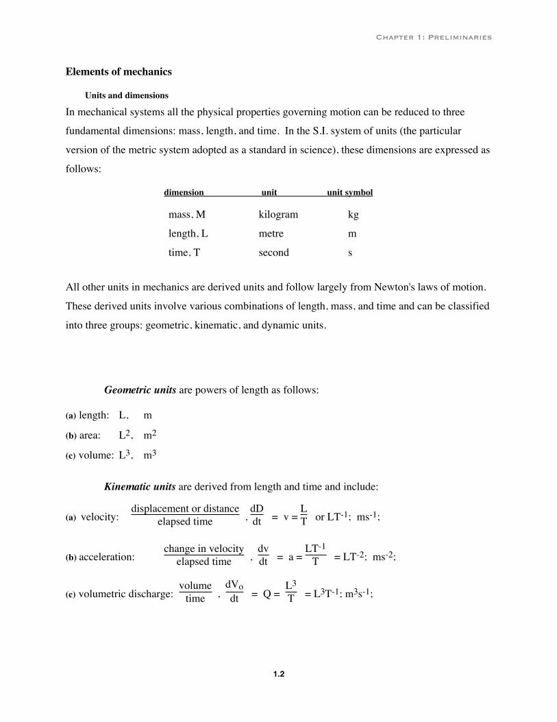
Geometric units are powers of length as follows:

(a) length: L, m

(b) area: L2, m2

(c) volume: L3, m3

Kinematic units are derived from length and time and include:

(a) velocity: displacement or distance

elapsed time , dDdt = v =

LT or LT-1; ms-1;

(b) acceleration: change in velocity

elapsed time , dvdt = a =

LT-1

T = LT-2; ms-2;

(c) volumetric discharge: volume

time , dVodt = Q =

L3

T = L3T-1; m3s-1;


1.3

Equations of uniformly accelerated motion

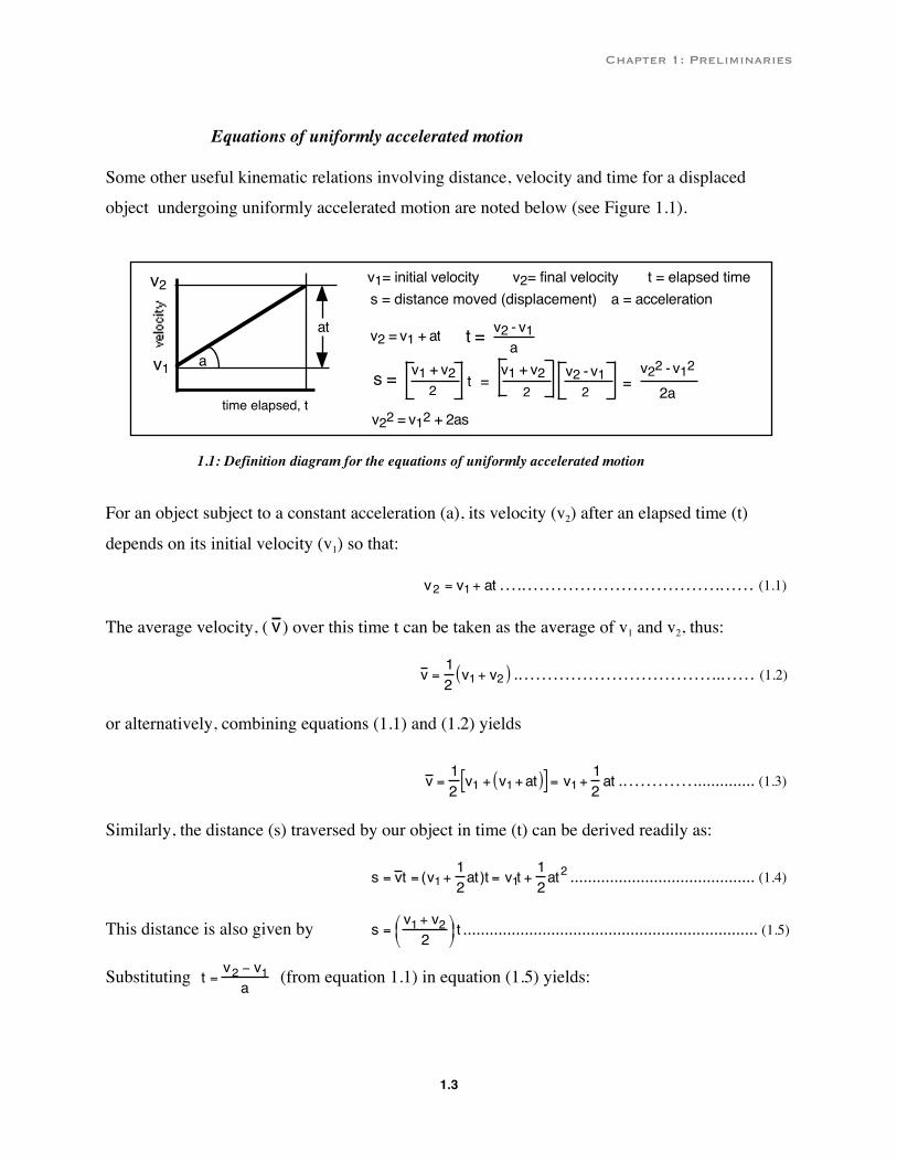
Some other useful kinematic relations involving distance, velocity and time for a displaced

object undergoing uniformly accelerated motion are noted below (see Figure 1.1).

1.1: Definition diagram for the equations of uniformly accelerated motion

For an object subject to a constant acceleration (a), its velocity (v2) after an elapsed time (t)

depends on its initial velocity (v1) so that:

v2 = v1+ at….…………………………….…… (1.1)

The average velocity, ( v ) over this time t can be taken as the average of v1 and v2, thus:

v = 12 v1+ v2( ) .……………………………..…… (1.2)

or alternatively, combining equations (1.1) and (1.2) yields

v = 12 v1 + v1+at( )[ ] = v1+

12 at .………….............. (1.3)

Similarly, the distance (s) traversed by our object in time (t) can be derived readily as:

s = v t = (v1+12 at)t = v1t +

12 at2 .......................................... (1.4)

This distance is also given by s =v1+ v22

t ................................................................... (1.5)

Substituting t = v2 − v1a (from equation 1.1) in equation (1.5) yields:

time elapsed, t

v2

v1 a

a = acceleration

at

v1= initial velocity v2= final velocitys = distance moved (displacement)

t = elapsed time

v2 = v1 + at t = v2 - v1a

s = v1 + v22 t = v2 - v1

2v1 + v2

2 = v22 - v12

2av22 = v12 + 2as


1.4

s =v1+ v22

v2 − v1a

=

v22 − v122a or by rearrangement, 2as = v22 − v12

and v22 = v12 + 2as ...............................................................……….. (1.6)

Dynamic units incorporate length, mass, and time and involve definitions which

flow from the principles of dynamics formulated by the remarkable 17th century physicist and

mathematician, Sir Isaac Newton, principles which we know as Newton’s Laws of Motion.

Newton’s first law of motion, a confirmation of Galileo’s earlier observation, states that every

body remains at rest, or continues to move with constant velocity in a straight line, unless acted

upon by a force. The first part of this law, relating to a body at rest, most of us treat as common

sense but the second part, relating to a body in motion, is an idea that is not intuitively obvious.

Our common experience is that all objects set in motion (a rolling ball or a sliding hockey puck,

for example) will come to rest because of friction. Newton recognized the retarding force of

friction and abstracted the ideal case where friction vanishes.

An object that does not change its state of motion is said to be in equilibrium. Again, the fact that

an object at rest is in equilibrium is a more comfortable notion to most of us than the idea that an

object moving at a constant velocity in a straight line also represents an equilibrium state. But in

physics both states are taken to represent equilibrium.

We all know intuitively what is meant by force: it is a push or pull acting on a body. It is in fact

anything that causes a body to change its state of motion. Force here means net force. An object

in motion is unaffected by equally opposed forces because net force, or simply impressed force,

is zero.

Newton’s second law of motion states that a force acting on a body produces an acceleration in

its motion; this acceleration is in the direction of the force; the force necessary to produce a

given acceleration is equal to the product of the acceleration and a factor m characteristic of the

body itself; this factor, called the mass of the body, is directly proportional to the amount of

matter contained in it. Whereas the first law describes the motion of bodies in the absence of


1.5

forces, this second law describes the cause and effect relation between forces and motion. It

relates the disequilibrium condition involving a change in velocity, or acceleration, to the net

force impressed on the body, and to its mass. Indeed, the law serves as the vehicle for defining

both force and the unit of force. Mathematically we say that:

F = ma ……………….……………………….…… (1.7)

The unit for mass is the kilogram (kg) and those for acceleration are ms-2 so force has the

dimensions MLT-2 and units kgms-2. This unit is named for Newton so from this definitional

equality we can say that a force of 1N acting on a 1 kg mass will accelerate it by 1 ms-2.

This definitional equality should also remind us that the common notion of weight is not the

same as the mass of an object. Weight on planet Earth is the force that a body exerts by virtue of

the combined properties of mass and the acceleration produced by the attraction of gravity

towards the centre of the planet. Mass is an inherent property of a particular body but its weight

will vary with the pull of gravity (and the resulting gravitational acceleration). Although

gravitational acceleration, g, can be taken as sensibly constant at 9.80 ms-2, everywhere on Earth,

the weight of a given object would vary greatly if it were measured on the moon or on other

bodies with a mass different from that of Earth.

Newton’s third law of motion, states that every action has an equal and opposite reaction. This

law states that that, when a body exerts a force on another, the second body exerts an equal and

oppositely directed force on the first. This law, like the first, formalizes a commonplace

observation: if you push an object it pushes back on your hand; if you support a weight on a

rope, the rope pulls down on your hand. Less intuitively obvious, but also true, is the force that a

table surface exerts upwards in supporting the weight of a book resting on it. We will see later

that there are important analogous circumstances involving the forces exerted by flowing water

on the bed of a river (and the reaction force exerted by the bed against these forces).

Dynamic units in this Newtonian physics framework that we will put to use in the pages ahead

are summarized below:


1.6

(a) density, ρ (mass per unit volume) =

€

ML3 = ML-3; kgm-3

(b) weight (mass x gravitational acceleration) = MLT-2; kgms-2 or kgf; note that 'weight' here is

not mass but rather a body force acquired by virtue of gravitational acceleration; see the

discussion above.

(c) force = Ma = MLT-2; kgms-2 (Newtons, N)

(d) specific weight = weight per unit volume

= force per unit volume = MLT-2L-3 = ML-2T-2; kgfm-3 or Nm-3

(e) pressure is force/area = MLT-2L-2 = ML-1T-2; kgfm-2 or Nm-2

(f) shear stress is a tangential force per unit area and has the same dimensions and units as

pressure (MLT-2L-2 = ML-1T-2; kgfm-2 or Nm-2)

(g) work is defined as the product of a force and the distance moved by the point of its

application in the direction of application:

work = Fd = MLT-2L = ML2T-2; Joules

If a force of 1 N acts over 1m, the work done is 1J (Joule). Note that changes in energy result in

work being done; thus energy and work have the same dimensions and units.

(h) potential energy, PE, is the energy a body possesses by virtue of its mass and height above

some arbitrary datum in the presence of a gravity field; PE so defined also is equivalent to the

work done in raising a body of mass M to a height h against gravity g:

PE = mgh = MLT-2L = ML2T-2; Joules

(i) kinetic energy, KE, is the energy a body possesses by virtue of its mass and velocity; KE is

also work done in accelerating mass m to some velocity v, so that

KE =

€

12

mv2 = M(LT-1)2 = ML2T-2, Joules

(j) power, P, is the rate of doing work or of expending energy:

P = Wt or

Et =

€

ML2T−2

T= ML2T-3 Watt (1 Watt = 1 Joule/second)


1.7

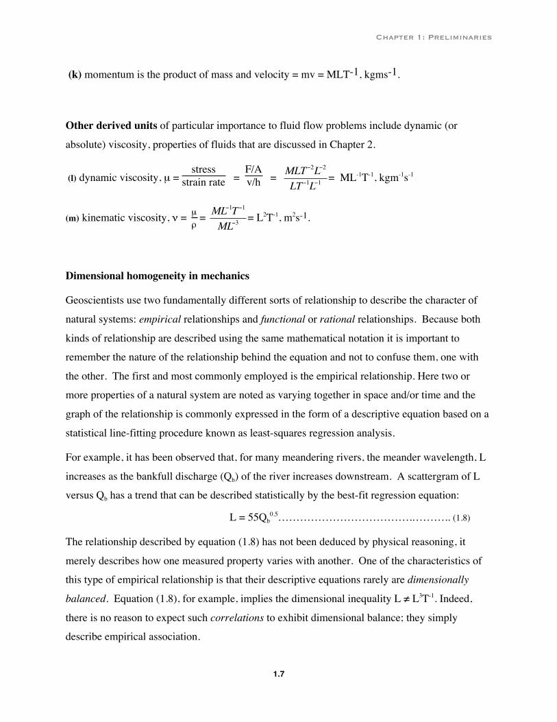
(k) momentum is the product of mass and velocity = mv = MLT-1, kgms-1.

Other derived units of particular importance to fluid flow problems include dynamic (or

absolute) viscosity, properties of fluids that are discussed in Chapter 2.

(l) dynamic viscosity, µ = stress

strain rate = F/Av/h =

€

MLT−2L−2

LT−1L−1= ML-1T-1, kgm-1s-1

(m) kinematic viscosity, ν = µρ

=

€

ML−1T−1

ML−3= L2T-1, m2s-1.

Dimensional homogeneity in mechanics

Geoscientists use two fundamentally different sorts of relationship to describe the character of

natural systems: empirical relationships and functional or rational relationships. Because both

kinds of relationship are described using the same mathematical notation it is important to

remember the nature of the relationship behind the equation and not to confuse them, one with

the other. The first and most commonly employed is the empirical relationship. Here two or

more properties of a natural system are noted as varying together in space and/or time and the

graph of the relationship is commonly expressed in the form of a descriptive equation based on a

statistical line-fitting procedure known as least-squares regression analysis.

For example, it has been observed that, for many meandering rivers, the meander wavelength, L

increases as the bankfull discharge (Qb) of the river increases downstream. A scattergram of L

versus Qb has a trend that can be described statistically by the best-fit regression equation:

L = 55Qb0.5……………………………….……….. (1.8)

The relationship described by equation (1.8) has not been deduced by physical reasoning, it

merely describes how one measured property varies with another. One of the characteristics of

this type of empirical relationship is that their descriptive equations rarely are dimensionally

balanced. Equation (1.8), for example, implies the dimensional inequality L ≠ L3T-1. Indeed,

there is no reason to expect such correlations to exhibit dimensional balance; they simply

describe empirical association.


1.8

The second type of relationship, the functional (or rational) relationship, is a physically based

relationship that describes the actual physical processes involved rather than just showing

empirical association. If an equation describing the relations among components of a physical

system is complete in the sense that all the relevant variables are included, then the equation

must be dimensionally balanced. If it is not balanced dimensionally then we conclude that the

equation is not structurally sound and needs to be modified. We should note that the 'if' in the

preceding sentence, however, is rarely satisfied in geomorphology because we can never be sure

that we have included all the relevant variables in what are typically quite complex systems. For

this reason functional equations are not as commonly encountered in geomorphology as are

empirical relations.

Nevertheless, in certain simple cases, such as open-channel flow problems, it may be possible to

propose a physically based relationship in which the criterion of complete specification of the

physical system is met. In such cases dimensional balance should apply.

For example, discharge, Q, through a conduit of cross-sectional area, A, is deduced to be Q = Av

where v is the average velocity. The discharge Q is expressed in terms of metres3/second and the

units of Av are formed from the product of A (metres2) and velocity (metres/second) or again,

metres3/second. Or to restate the case in basic dimensions:

Q = A v

L3T-1 L2 LT-1 = L3T-1

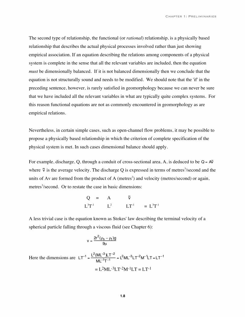
A less trivial case is the equation known as Stokes' law describing the terminal velocity of a

spherical particle falling through a viscous fluid (see Chapter 6):

v = 2r2(ρs − ρf )g

9µ

Here the dimensions are LT−1 = L2(ML−3 )LT−2

ML−1T−1= L2ML−3LT−2M−1LT =LT−1

= L2ML-3LT-2M-1LT = LT-1


1.9

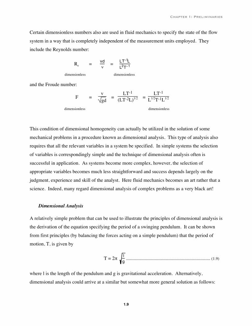
Certain dimensionless numbers also are used in fluid mechanics to specify the state of the flow

system in a way that is completely independent of the measurement units employed. They

include the Reynolds number:

Re = vdν

= LT−1LL2T−1

dimensionless dimensionless

and the Froude number:

F = vgd =

LT-1

(LT-2L)1/2 = LT-1

L1/2T-1L1/2

dimensionless dimensionless

This condition of dimensional homogeneity can actually be utilized in the solution of some

mechanical problems in a procedure known as dimensional analysis. This type of analysis also

requires that all the relevant variables in a system be specified. In simple systems the selection

of variables is correspondingly simple and the technique of dimensional analysis often is

successful in application. As systems become more complex, however, the selection of

appropriate variables becomes much less straightforward and success depends largely on the

judgment, experience and skill of the analyst. Here fluid mechanics becomes an art rather that a

science. Indeed, many regard dimensional analysis of complex problems as a very black art!

Dimensional Analysis

A relatively simple problem that can be used to illustrate the principles of dimensional analysis is

the derivation of the equation specifying the period of a swinging pendulum. It can be shown

from first principles (by balancing the forces acting on a simple pendulum) that the period of

motion, T, is given by

T = 2π lg .................................................................... (1.9)

where l is the length of the pendulum and g is gravitational acceleration. Alternatively,

dimensional analysis could arrive at a similar but somewhat more general solution as follows:


1.10

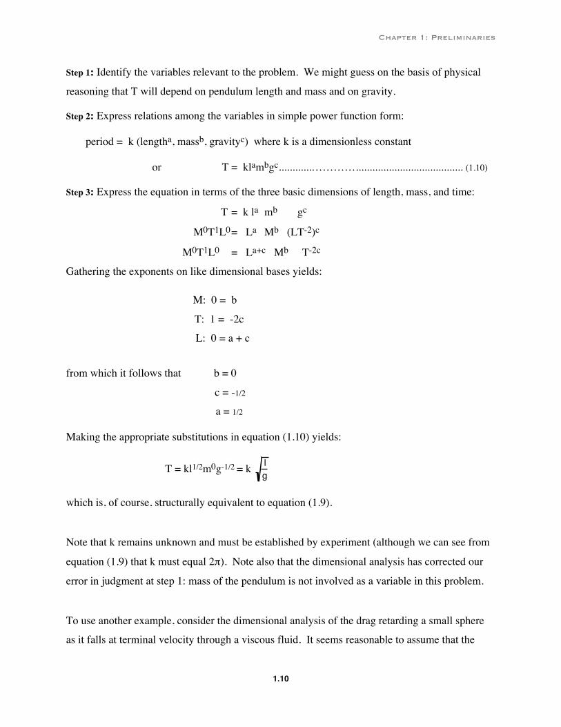
Step 1: Identify the variables relevant to the problem. We might guess on the basis of physical

reasoning that T will depend on pendulum length and mass and on gravity.

Step 2: Express relations among the variables in simple power function form:

period = k (lengtha, massb, gravityc) where k is a dimensionless constant

or T = klambgc............…………....................................... (1.10)

Step 3: Express the equation in terms of the three basic dimensions of length, mass, and time:

T = k la mb gc

M0T1L0 = La Mb (LT-2)c

M0T1L0 = La+c Mb T-2c

Gathering the exponents on like dimensional bases yields:

M: 0 = b

T: 1 = -2c

L: 0 = a + c

from which it follows that b = 0

c = -1/2

a = 1/2

Making the appropriate substitutions in equation (1.10) yields:

T = kl1/2m0g-1/2 = k lg

which is, of course, structurally equivalent to equation (1.9).

Note that k remains unknown and must be established by experiment (although we can see from

equation (1.9) that k must equal 2π). Note also that the dimensional analysis has corrected our

error in judgment at step 1: mass of the pendulum is not involved as a variable in this problem.

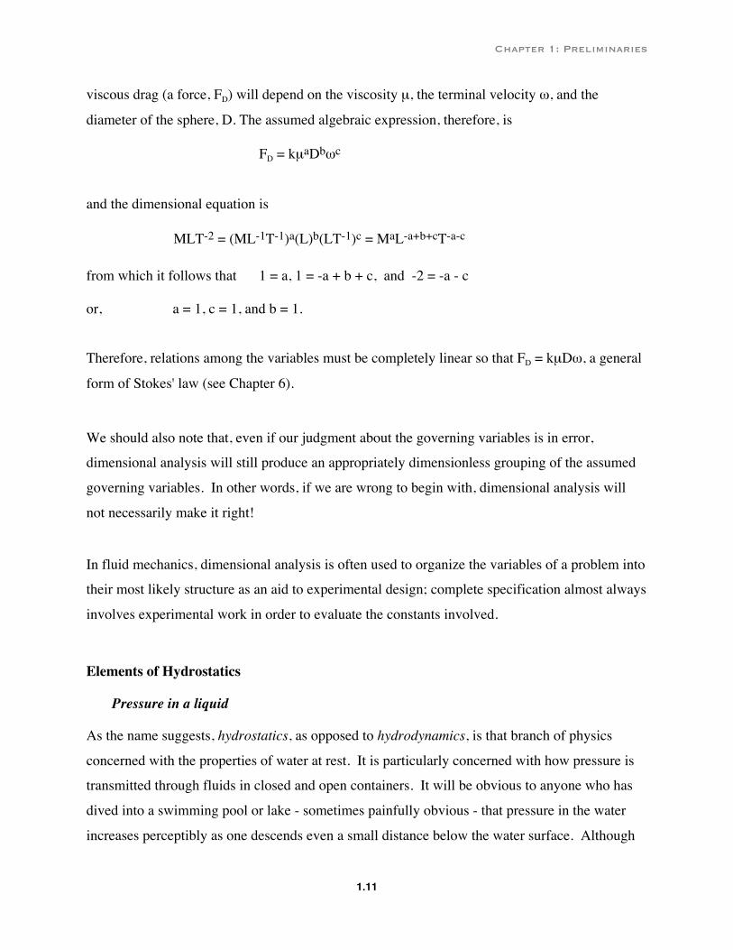
To use another example, consider the dimensional analysis of the drag retarding a small sphere

as it falls at terminal velocity through a viscous fluid. It seems reasonable to assume that the


1.11

viscous drag (a force, FD) will depend on the viscosity µ, the terminal velocity ω, and the

diameter of the sphere, D. The assumed algebraic expression, therefore, is

FD = kµaDbωc

and the dimensional equation is

MLT-2 = (ML-1T-1)a(L)b(LT-1)c = MaL-a+b+cT-a-c

from which it follows that 1 = a, 1 = -a + b + c, and -2 = -a - c

or, a = 1, c = 1, and b = 1.

Therefore, relations among the variables must be completely linear so that FD = kµDω, a general

form of Stokes' law (see Chapter 6).

We should also note that, even if our judgment about the governing variables is in error,

dimensional analysis will still produce an appropriately dimensionless grouping of the assumed

governing variables. In other words, if we are wrong to begin with, dimensional analysis will

not necessarily make it right!

In fluid mechanics, dimensional analysis is often used to organize the variables of a problem into

their most likely structure as an aid to experimental design; complete specification almost always

involves experimental work in order to evaluate the constants involved.

Elements of Hydrostatics

Pressure in a liquid

As the name suggests, hydrostatics, as opposed to hydrodynamics, is that branch of physics

concerned with the properties of water at rest. It is particularly concerned with how pressure is

transmitted through fluids in closed and open containers. It will be obvious to anyone who has

dived into a swimming pool or lake - sometimes painfully obvious - that pressure in the water

increases perceptibly as one descends even a small distance below the water surface. Although


1.12

we may sense in such a submerged state that the water is “pressing down” on us, the pressure at a

point in the water actually acts uniformly in all directions. The fact that standing water, by

definition, does not flow implies that this must be so. Consider an imaginary small cube of water

at depth; Newton’s second law of motion tells us that, since the velocity of the cube is zero, it

must be the case that the force per unit area (the pressure) acting on each face is balanced by the

same opposing pressure on the opposite face so that the resultant of force acting on all faces, the

net force, is also zero.

Figure 1.2 shows (a) a cylinder of liquid with a free water-surface, and (b) the contained water as

a free body in equilibrium for which the container is replaced by the forces its walls exert on the

fluid. Two forces act together vertically downward and by Newton’s third law, are equal to the

upward-directed force supporting the liquid cylinder P’hA (where P’ is the pressure exerted on

the lower face of the free body at a depth h below the water surface). The two forces acting

downward are the result of atmospheric pressure (PAA where PA is atmospheric pressure and A is

the area of the water surface) and the weight (W) of the cylindrical volume of water (W = mg

=ρVg = ρAhg).

Hence, we can state formally that:

€

P'h = PAA + ρghA ...................... (1.11)

Equation (1.11) indicates that the

pressure in excess of the atmospheric

pressure at depth h below the liquid

surface is directly proportional to

gravitational acceleration (g), the

density of the liquid (ρ), and the depth

of the liquid (h). This linear

proportionality with depth differs from 1.2: Definition diagram for forces acting on a cylinder of liquid

h

Free-body diagram of the liquid in the cylinder (a)

P AA

W = Ahgρ

P' Ah

h

a b

Cylinder containing a liquid of density filled to a height h ρ


1.13

the corresponding relation for gasses. Because gasses are compressible, the weight of a similar

column of gas results in compression of the gas with depth and density increases exponentially

with depth. Our case, however, is much simpler. The sensibly incompressible nature of water

means that, for all practical purposes, the average hydrostatic pressure in a column of water

occurs at h/2. It also follows from equation (1.1) that the difference in pressure between two

points whose depths differ by Δh is:

€

ΔP = ρgΔh ..................................................... (1.12)

In most problems in the fluid mechanics of open-channel flow we are

concerned only with pressure differences so that atmospheric pressure is

ignored in practice.

Pascal’s Principle states that, under equilibrium conditions, a change in

pressure at any point in an incompressible fluid is transmitted uniformly

to all parts of the fluid. This important principle is illustrated in Figure

1.3. Here an elbow-shaped cylinder is filled with liquid to a height h.

Although the depth of water above point B in the horizontal part of the

elbow is equal only to the cylinder diameter, d, Pascal’s principle dictates

that the pressure here must be equal to that at point A (PAA + ρghA). If

this were not the case, of course, the fluid would flow along the pressure

gradient from point A to B. Pascal’s principle is put to good use in

hydraulic machines although we will not be concerned with that

application here.

Buoyancy is a force which, when we are swimming, we experience as

the familiar tendency to float. Submerged objects such as boat anchors

are more easily raised through the water to the surface than from the

water surface to the boat because of the greater buoyant lift given by

water. It is the same force that lifts a helium-filled weather balloon

through the air.

This upward buoyant force is exerted on a submerged object because the

hydrostatic pressure at the base of the object is greater than that on its

A B

h d

water surface

1.3: Pascal's principle dictates that pressures at points A and B are equal.

T

mg

p1

p2

1.4: Forces acting on a submerged cylinder suspended by a wire under tension, T

h


1.14

upper surface above which the depth of water is lower. Consider the small solid cylinder

suspended in a liquid by a support wire as shown in Figure 1.4. Equation (1.12) indicates that the

difference in hydrostatic pressure between the top and the base of the cylinder must be

ΔP =ρgΔh= ρgh where h is the height of the submerged cylindrical object. Thus the difference in

the upward force acting on the lower surface and the downward force acting on the upper surface

(the buoyant force, FB) must have a magnitude given by:

€

ΔPA = FB = ρghA =WL ................................................. (1.5)

where ρ is the density of the liquid. Clearly, the buoyant force FB is equal to the weight (WL) of

the water displaced by the submerged cylinder.

Archimedes’ Principle, the fundamental law of hydrostatics illustrated by this example, states

that a body completely or partially submerged in a fluid is buoyed up by a force equal to the

weight of the fluid it displaces. As we will see in Chapter 6, Archimedes’ principle is an

important factor in any consideration of the forces acting on submerged grains resting on the bed

of a river. The submerged weight of such a grain must be discounted by the buoyant force so

that its immersed weight W is given by:

€

W =Vg(ρs − ρw ) ........................................................... (1.6)

where V is the particle volume and ρs and ρw are respectively the density of the sediment particle

and of the water.

Measurement: significant figures and uncertainty

Whether we are concerned with the density of a solid, or the velocity of flowing water or the

hydrostatic pressure in a water column, our observations must be expressed in quantitative form

based on primary measurements and on derived expressions based on manipulation of these

measurements. Now that we all routinely use increasingly powerful calculators and computers

which in a few milliseconds produce eight or more decimal places for any and all kinds of

calculation, it is more important than ever to remind ourselves of the real meaning of all that

apparent computing power and precision! Here is also a good place to consider the effects of

uncertainties in our measurements as they are propagated through the equations we employ to

solve numerical problems in fluvial geomorphology.


1.15

Significant figures

Although our calculators and computers carry computations to eight or more decimal places the

final results are only as accurate as the original measurements on which they are based.

Obviously your calculator cannot refine a measurement although it is quite easy to overlook this

basic limitation on the accuracy of measurements when a lot of numerical manipulation is

involved in solving a problem.

Suppose you are asked to find out how long it would take an object moving at a velocity of 7.1

ms-1 to travel a distance of 6 m. The solution on a typical calculator is 6 ÷ 7.1 = 0.8450704 s.

Obviously this many decimal places is meaningless since one of the original elements, namely 6

m, was only measured accurately as a whole number. The best answer you can report is that the

time of travel is 0.8 s.

Again, suppose that you have to measure the length of a pencil with a ruler divided into

centimetre and millimetre divisions. Your initial measurement is 15.5 cm but you decide that a

more precise measurement is required and you repeat the exercise with the aid of a magnifying

glass that enables you to estimate that the pencil length is between 15.56 cm and 15.58 cm. Thus,

you report the length as 5.57 cm. The last digit, although somewhat doubtful, is significant

because it tells us something about the accuracy of your measurement device (the ruler scale)

and something about your ability to use it. Your measurement of 15.57 cm therefore has four

significant figures. If you wish to report this measurement in metres (0.1557 m) or in

millimetres (155.7 mm) the number of significant figures is still four.

Note that the zero to the left of the decimal place in 0.1557 m merely helps mark the place of the

decimal point and does not count as a significant figure. In contrast, the zero in a velocity

measurement of 1.02 ms-1 is a significant figure so we can say that the measurement has three

significant figures.

In some cases zeros are used only to express the size of a number, and are not significant. For

example, the speed of light in a vacuum has been measured as 299 800 000 ms-1. Here the

structure of the number tells you something about the accuracy of the measurement; it is

indicated more clearly using scientific notation: 2.998 x 108 ms-1. Thus, we can see that this


1.16

particular measurement of the speed of light has four significant figures.

Arithmetic operations must also respect the numbers of significant figures in the elements

involved. For example, if we add 2.41 (three significant figures; doubtful number in bold) to

7.118 (four significant figures), the result is 9.528. Since it makes sense to indicate only the last

digit as doubtful, we round up the final digit from 2 to 3 and report the result as 9.53. The same

rule applies to multiplication and division. A rule of thumb here is that the result cannot have

more significant figures than the least accurate of the elements, so that, for example, 2.2 x 3.007

= 6.6, not 6.615. An exception to this rule, of course, is when the number of digits to the left of

the decimal point increases as a result of addition: for example, 9.6 + 1.97 = 11.57 would be

reported as 11.6. This result has three significant figures even though one of the original

elements (9.6) has only two.

Uncertainty in measurements

No physical measurement is 'exact' and it often is useful to have an indication of the uncertainty

involved. In the earlier example where the pencil was reported as being 15.57 cm long, we could

say with certainty that it was not less than 15.56 cm but not longer than 15.8 cm. In effect we are

reporting that the length is 15.57 ± 0.01 cm. This uncertainty (or error) in the measurement is a

random error because there is equal probability that a given measurement will be greater or less

than 15.57 cm. Also the absolute deviation from 15.57 cm will vary from measurement to

measurement depending on variable operator performance (the 'human factor'). Because these

random errors are the product of chance, we reduce their effect by taking large numbers of

measurements and taking the average value. The ± error associated with the average value can

then be expressed as a standard deviation of the measurements in the set or sample.

In addition to random errors, measurement uncertainty may include systematic errors.

Systematic errors are always either positive or negative and therefore bias the result in a

particular direction. Such errors include instrument effects where, for example, a drift off

calibration produces measurements which are consistently too high or too low. In our pencil

length example, a distorted scale on the ruler would produce a systematic error. They may

involve operator bias (for example, a consistent tendency to lean to the right when reading the

ruler scale would produce a systematic parallax effect) or some external influence such as

temperature or humidity.


1.17

It is important to recognize and eliminate systematic errors during the course of an experiment or

field survey although in practice random and systematic errors are sometimes difficult to

distinguish one from the other.

The propagation of errors

Although uncertainties or errors in individual measurements may be assessed at the time of

measurement, their interactive effects in subsequent computations are not intuitively obvious.

The rules for propagation of errors in formulae involving addition, subtraction, multiplication,

division, and powers, are examined below. There are additional rules for other operations such

as those involving trigonometric functions but these will not be considered here. If you are

interested in pursuing this topic further you should consult one of the many texts on error

analysis (there are some suggestions in the references).

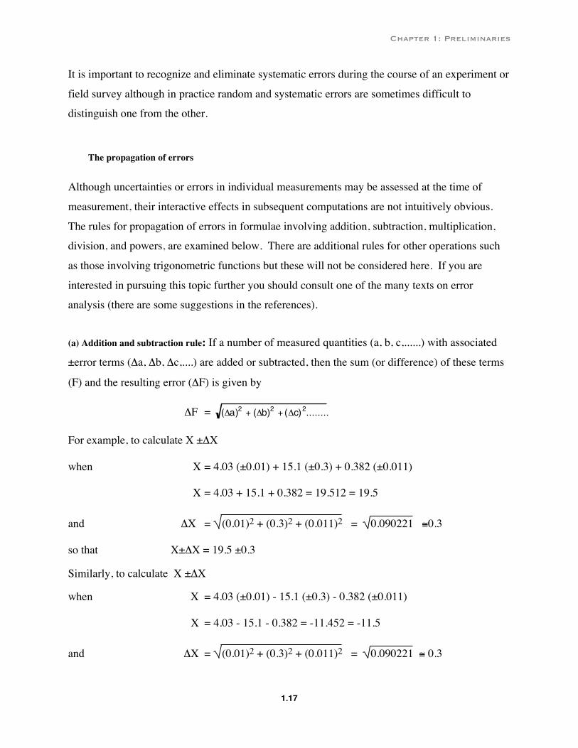
(a) Addition and subtraction rule: If a number of measured quantities (a, b, c,......) with associated

±error terms (Δa, Δb, Δc,....) are added or subtracted, then the sum (or difference) of these terms

(F) and the resulting error (ΔF) is given by

ΔF = (Δa)2 + (Δb)2 + (Δc)2........

For example, to calculate X ±ΔX

when X = 4.03 (±0.01) + 15.1 (±0.3) + 0.382 (±0.011)

X = 4.03 + 15.1 + 0.382 = 19.512 = 19.5

and ΔX = (0.01)2 + (0.3)2 + (0.011)2 = 0.090221 ≅0.3

so that X±ΔX = 19.5 ±0.3

Similarly, to calculate X ±ΔX

when X = 4.03 (±0.01) - 15.1 (±0.3) - 0.382 (±0.011)

X = 4.03 - 15.1 - 0.382 = -11.452 = -11.5

and ΔX = (0.01)2 + (0.3)2 + (0.011)2 = 0.090221 ≅ 0.3


1.18

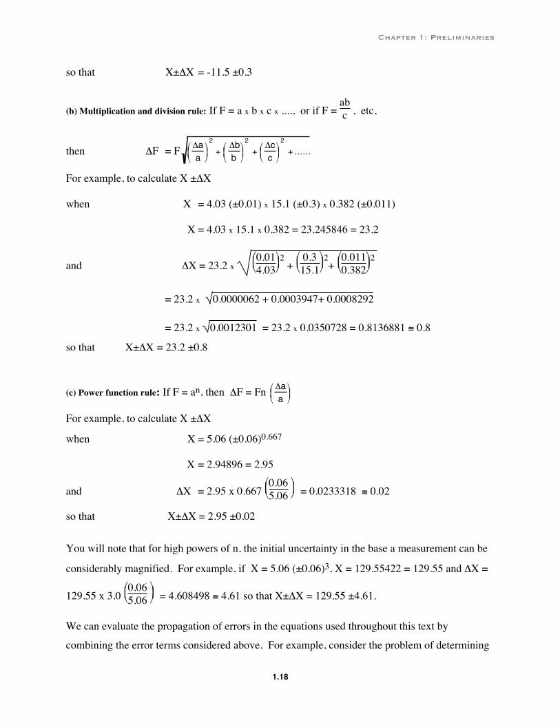
so that X±ΔX = -11.5 ±0.3

(b) Multiplication and division rule: If F = a x b x c x ...., or if F = abc , etc,

then ΔF = F Δaa

2

+Δbb

2

+Δcc

2

+ ......


when X = 4.03 (±0.01) x 15.1 (±0.3) x 0.382 (±0.011)

X = 4.03 x 15.1 x 0.382 = 23.245846 = 23.2

and ΔX = 23.2 x

0.01

4.032 +

0.3

15.12+

0.011

0.3822

= 23.2 x 0.0000062 + 0.0003947+ 0.0008292

= 23.2 x 0.0012301 = 23.2 x 0.0350728 = 0.8136881 ≅ 0.8

so that X±ΔX = 23.2 ±0.8

(c) Power function rule: If F = an, then ΔF = Fn Δaa


when X = 5.06 (±0.06)0.667

X = 2.94896 = 2.95

and ΔX = 2.95 x 0.667

0.06

5.06 = 0.0233318 ≅ 0.02

so that X±ΔX = 2.95 ±0.02

You will note that for high powers of n, the initial uncertainty in the base a measurement can be

considerably magnified. For example, if X = 5.06 (±0.06)3, X = 129.55422 = 129.55 and ΔX =

129.55 x 3.0

0.06

5.06 = 4.608498 ≅ 4.61 so that X±ΔX = 129.55 ±4.61.

We can evaluate the propagation of errors in the equations used throughout this text by

combining the error terms considered above. For example, consider the problem of determining


1.19

the uncertainty in the magnitude of roughness n computed from Manning's equation if the

following measurement errors apply:

water surface slope, s = 0.005 ±0.001

mean flow depth, d = 2.00 ±0.30 m

mean flow velocity, v = 2.00 ±0.20 ms-1

The Manning equation states that:

n =

€

d2 / 3s1/ 2

v= 2.00

2 / 30.0051/ 2

2.00= 0.06 ±Δn

We deal with the errors in the order of the operations involved, powers first followed by the

multiplication and division. In the case of d2/3, we know from the power function rule [F = an;

ΔF = Fn Δaa

] that the uncertainty in (2.0 ±0.3)2/3 is ΔF = (2.0)2/3

2

3

0.3

2.0 = 0.15874. Note

that you can carry as many decimals through the calculations as you fancy, provided the final

result is reported with the correct number of significant figures.

Entering the uncertainty for d2/3 in the Manning equation yields:

n = (1.5874 ±0.15874)s1/2

v

The uncertainty in the other power function, s1/2, is obtained in the same way so that

ΔF = (0.005)1/2 1

2

0.001

0.005 = 0.00707.

Entering this value for s1/2 and the specified uncertainty in v (2.00±0.2) in the Manning equation

yields:

n = (1.5874 ± 0.15874)(0.0707 ± 0.007)2.00 ± 0.2

The uncertainty in n can now be evaluated by using the rule for multiplication and division:

Δn = (1.5874)(0.0707)

(2.0)0.158741.5874

2

+0.0070.0707

2

+0.202.00

2

= 0.009687 =0.01

So we can report the calculated value of n together with its uncertainty Δn, as


1.20

n = 0.06 ±0.01

Concluding Remarks

We have just touched on the topics of this chapter sufficient to serve our immediate needs in the

pages to follow. If you would like to explore further such topics as dimensional analysis and

error analysis there are several excellent sources listed in the references for this chapter that you

might like to explore. Meanwhile, we must turn our attention to the application of Newton’s

laws of motion to fluids moving through channels with rigid boundaries.

References

Blatt, F.J., 1989, Principles of Physics, Allyn and Bacon, Boston.

College Physics Hypertextbook: http://www.rwc.uc.edu/koehler/biophys/text.html

University of Guelph, Physics Tutorials: http://www.physics.uoguelph.ca/tutorials/tutorials.html

some preliminaries elements of mechanics dimensional homogeneity in mechanics elements of

Documents