some questions in algebraic geometry (vector bundles, normal
TRANSCRIPT

UNIVERSITY OF FERRARA
PHD IN MATHEMATICS AND COMPUTER SCIENCE
CICLO XXIV
Some questions in algebraic geometry(vector bundles, normal bundles and fat points)
S.S.D. MAT/03
Advisor:
Chiar.mo Prof.
Philippe Ellia
Phd candidate:
Ludovica Chiodera
2009-2011

Contents
Introduction iii
1 Rank two globally generated vector bundles with c1 ≤ 5. 1
1.1 General facts. . . . . . . . . . . . . . . . . . . . . . . . . . . . . . . . 1
1.2 Globally generated vector bundle on Pn, with c1 = 0 . . . . . . . . . . 3
1.3 Globally generated vector bundles on Pn, with c1 = 1. . . . . . . . . . 5
1.4 A general result. . . . . . . . . . . . . . . . . . . . . . . . . . . . . . 8
1.5 Globally generated vector bundles on Pn with c1 = 2. . . . . . . . . . 16
1.6 Globally generated rank two vector bundles on Pn, n ≥ 3, with c1 ≤ 5. 21
1.6.1 Globally generated rank two vector bundles on P3 with c1 = 3. 21
1.6.2 Globally generated rank two vector bundles on P3 with c1 = 4. 22
1.6.3 Globally generated rank two vector bundles on P3 with c1 = 5. 26
1.6.4 Globally generated rank two vector bundles on Pn, n ≥ 4 with
c1 ≤ 5. . . . . . . . . . . . . . . . . . . . . . . . . . . . . . . . 29
2 On the normal bundle of projectively normal space curves. 31
2.1 Basic facts on a.C.M. curves. . . . . . . . . . . . . . . . . . . . . . . . 31
2.2 A conjecture on the normal bundle. . . . . . . . . . . . . . . . . . . . 35
2.3 Numerical characters and the inequality (∗s). . . . . . . . . . . . . . 39
2.4 Double structures and normal bundle. . . . . . . . . . . . . . . . . . . 41
2.5 Some general results. . . . . . . . . . . . . . . . . . . . . . . . . . . . 46
2.6 Small values of s and conclusion. . . . . . . . . . . . . . . . . . . . . 50
2.7 Appendix . . . . . . . . . . . . . . . . . . . . . . . . . . . . . . . . . 53
i
ii CONTENTS
3 Subschemes of P2 with ten fat point of maximum rank. 75
3.1 Subschemes of P2 with fat point. . . . . . . . . . . . . . . . . . . . . 75
3.2 Special linear systems of plane curves. . . . . . . . . . . . . . . . . . 77
3.3 The Horace's method. . . . . . . . . . . . . . . . . . . . . . . . . . . 82
3.4 Horace dierential's method and collision of innitesimal neighborhood. 86
3.5 Cremona transformations. . . . . . . . . . . . . . . . . . . . . . . . . 100
3.6 Subschemes of P2 with ten fat points of multiplicity less than nine. . . 102

Introduction
In the rst chapter we deal with rank two globally generated vector bundles with
c1 ≤ 5 on Pn, where c1 indicates the rst Chern class of vector bundle. We classify
this bundles through their Chern class. To do it, we use the lemma 1.1.6 and 1.1.8,
in particulary on P3 we play on the following remark 1.1.9
Remark 0.0.1 If E is a globally generated rank two vector bundle on P3 we have
an exact sequence:
0→ O → E → IC(t)→ 0
where t = c1(E) and where C is a smooth curve. It follows that C is linked to a
smooth curve, X, by a complete intersection (t, t). Moreover if h1(E(−t)) = 0, then
C is irreducible and then, if h1(IC(2t− 4)) = 0, X also is irreducible.
The last assertion follows from the liaison formula: if C,X are two curves in P3
linked by a complete intersection of type (a, b), then:
h1(IX(k)) = h1(IC(a+ b− k − 4)),∀k ∈ Z.
In the end we summarize our classication with the following theorem 1.6.30:
Theorem 0.0.2 Let E be a rank two vector bundle on Pn, n ≥ 3, generated by
global sections with Chern classes c1, c2, c1 ≤ 5.
1. If n ≥ 4, then E is the direct sum of two line bundles
2. If n = 3 and E is indecomposable, then
(c1, c2) ∈ S = ((2, 2), (4, 5), (4, 6), (4, 7), (4, 8), (5, 8), (5, 10), (5, 12).
iii

iv INTRODUCTION
If E exists there is an exact sequence: 0 → O → E → IC(c1) → 0 (∗), whereC ⊂ P3 is a smooth curve of degree c2 with ωC(4− c1) ' OC. The curve C is
irreducible, except maybe if (c1, c2) = (4, 8): in this case C can be irreducible
or the disjoint union of two smooth conics.
3. For every (c1, c2) ∈ S, (c1, c2) 6= (5, 12), there exists a rank two vector bundle
on P3 with Chern classes (c1, c2) which is globally generated (and with an exact
sequence as in (2)).
In the second chapter we study the normal bundle of projectively normal curves.
More precisely there is a conjecture (see Conj.2.2.2), due to Hartshorne, which
predicts when a "suciently" general projectively normal curve of invariants (d, g, s)
should have a semi-stable normal bundle. We rst reformulate in a more precise way
this conjecture (see Conj. 2.2.3, Conj. 2.2.4).
Then we generalize a little bit the method of [8] (see Prop. 2.4.7, Corollary
2.4.12) and prove the conjecture in some special cases (see Theorem 2.6.3).
In the last chapter we deal with subschemes of P2 with fat points. In particulary
given Z subscheme of P2, we want to calculate the dimension of linear system of
plane curves of degree d that contained Z. This problem is connect to speciality
of linear system. About this argument there exists a conjecture due to Harbourne-
Hirschowitz (see Conjecture 3.2.4) which predicts that a linear system of plane
curve L, with general multiple base points is special if and only if there exists an
exceptional curve with multiplicity at least two in the base locus. This conjecture
is partial proved by Ciliberto-Miranda (see Theorem 3.2.9) and by S. Yang (see
Theorem 3.2.10). We improved this results with the proposition 3.6.1:
Proposition 0.0.3 The conjecture of Harbourne-Hirschowitz holds in all the linear
system LZ(v), where Z = (b1P1 + ...+ bnPn) is a subscheme of P2, with n ≤ 10 and
bi ≤ 8 for all i = 1, ..., n, and v is its critical value.
Moreover we prove that every analyzed subscheme is of maximum rank (see
Theorem 3.6.4):
Theorem 0.0.4 Every subscheme of P2 in the form Z = (b1P1 + ... + bnPn) with
n ≤ 10 and 4 ≤ bi ≤ 8 for all i = 1, ..., n, is of maximum rank.
Chapter 1
Rank two globally generated vector
bundles with c1 ≤ 5.
1.1 General facts.
We recall (without proofs) some denitions and some well-known general facts we
will use in the sequel.
Definition 1.1.1 A coherent sheaf, F , on the projective scheme X is globally
generated (or generated by global sections) if the natural morphism of evaluation:
ev : H0(F)⊗OX → F is surjective.
Remark 1.1.2 In case F is locally free and globally generated, the kernel of ev is
also locally free.
The next lemma almost follows from the denition:
Lemma 1.1.3 Let F ,G be two coherent sheaves on the projectve scheme X. If F is
globally generated and if there exists a surjective morphism F → G → 0, then G is
globally generated. In particular if Y ⊂ X is a subscheme, F|Y is globally generated
if F is.
Let E be a rank r vector bundle on Pn. According to a famous theorem, for every
line L ⊂ Pn there is an r-uple aE(L) = (a1(L), ..., ar(L)) ∈ Zr; a1(L) ≥ ... ≥ ar(L)
1

2 1. Rank two globally generated vector bundles with c1 ≤ 5.
such that
EL ∼= OL(a1(L))⊕ ...⊕OL(ar(L)).
We have c1(E) =r∑i=1
ai(L).
Moreover if E is globally generated, then ai(L) ≥ 0,∀i (apply Lemma 1.1.3). In
particular c1(E) ≥ 0 for every globally generated vector bundle on Pn.The r-uple aE(L) ∈ Zr is called the splitting type of E on L.
Let G(1, n) be the Grassmannian of lines in Pn and dene a map:
aE : G(1, n)→ Zr : L→ aE(L)
by semi-continuity there is a dense open subset U ⊂ G(1, n) such that aE is constant
on U , the corresponding splitting type (i.e. the one of L ∈ U) is called the generic
splitting type of E. If U = G(1, n) (i.e. if aE is constant), the vector bundle E is
said to be uniform.
Lemma 1.1.4 Let E be a globally generated rank r vector bundle on Pn. If r > n
there is an exact sequence:
0→ (r − n).O → E → F → 0
where F is a rank n vector bundle generated by global sections.
Proof 1.1.5
See [18] o4, Lemma 4.3.1.
Lemma 1.1.6 Let E be a rank two vector bundle on Pn. If E is globally generated
then a general section of E vanishes along a smooth codimension two subscheme.
Proof 1.1.7
See [14].
We shall also need the following:
Lemma 1.1.8 Let C ⊂ P3 be a smooth curve. If IC(k) is globally generated and if S
and S ′ are suciently general in H0(IC(k)), the complete intersection S ∩ S ′ linksC to a smooth curve.

1.2 Globally generated vector bundle on Pn, with c1 = 0 3
Remark 1.1.9 If E is a globally generated rank two vector bundle on P3 we have
an exact sequence:
0→ O → E → IC(t)→ 0
where t = c1(E) and where C is a smooth curve. It follows that C is linked to a
smooth curve, X, by a complete intersection (t, t). Moreover if h1(E(−t)) = 0, then
C is irreducible and then, if h1(IC(2t− 4)) = 0, X also is irreducible.
The last assertion follows from the liaison formula: if C,X are two curves in P3
linked by a complete intersection of type (a, b), then:
h1(IX(k)) = h1(IC(a+ b− k − 4)),∀k ∈ Z.
Finally we recall Horrocks criterion for a vector bundle to split:
Theorem 1.1.10 (Horrocks)
A rank r vector bundle E on Pn is a direct sum of line bundles (E 'r⊕i=1
O(ai)) if
and only if hi(E(m)) = 0, 1 ≤ i ≤ n− 1 and all m ∈ Z.
As a corollary we have:
Proposition 1.1.11 Let E be a rank r vector bundle on Pn, n > 2. Then E 'r⊕i=1
O(ai) if and only if there exists a plane Π ⊂ Pn such that: EΠ 'r⊕i=1
OΠ(ai).
Proof 1.1.12
See [18] Chap. I, 2.3.
1.2 Globally generated vector bundle on Pn, withc1 = 0
In this section we recall the classication of globally generated vector bundles with
c1 = 0. This is well known and follows directly from a more general result of Van
de Ven on uniform vector bundles, here we provide an elementary direct proof.
4 1. Rank two globally generated vector bundles with c1 ≤ 5.
Lemma 1.2.1 Let E be a rank r vector bundle on P2, with c1(E) = 0. If E is
generated by global sections then E is trivial (E ' r.O).
Proof 1.2.2
Let's rst proof that E has a nowhere vanishing section.
Let L ⊂ P2 be a line, then by Grothendieck theorem EL splits. We have EL =
OL(a1)⊕ ...OL(ar); since EL (being a quotient of E) is generated by global sections,
ai ≥ 0, ∀i. Since c1(E) = 0 =∑ai, it follows that ai = 0,∀i i.e. EL = rOL. We
note that the bundle E splits in the same way for all lines of P2, hence E is a uniform
bundle. Since E is generated by global sections, there exists a non zero section s and
if L is general, sL 6= 0. We have sL = (λL1 , ..., λLr ), where the λLi are constants. Since
sL 6= 0, (λL1 , ..., λLr ) 6= (0, ..., 0). Suppose that s vanishes at a point p ∈ P2, consider
a line D through p. As before sD = (λD1 , ..., λDr ), but since sD(p) = 0, λDi = 0, ∀i.
Now consider the point q = L ∩ D, we must have (λ1L,..., λLr ) = (λD1 , ..., λ
Dr ) and
we get a contradiction. We conclude that s is nowhere vanishing hence yields an
injective morphism of vector bundles: 0→ O → E, it follows that we have an exact
sequence:
(∗∗) 0→ O → E → F → 0
where F is a rank (r − 1) vector bundle. Moreover c1(F ) = c1(E) = 0 and F , being
a quotient of E, is globally generated. Let's conclude the proof by induction on r. If
r = 1 there is nothing to prove. Assume the statement holds for r − 1. It follows
that F ' (r − 1).O. The exact sequence (∗∗) belongs to
Ext1(F,O) ' (r − 1).H1(O), since h1(O) = 0, the exact sequence splits. So E =
O ⊕ F = r.O.
Proposition 1.2.3 Let E be a vector bundle of rank r on Pn, generated by global
sections and with c1(E) = 0. Then E is trivial.
Proof 1.2.4
We prove the prop by induction on n. The case n = 1 is clear and the case n = 2
is Lemma 1.2.1. Let's assume n > 2. Let Π ⊂ Pn be a plane. We have c1(EΠ) = 0
and EΠ is generated by global sections. By Lemma 1.2.1, EΠ ' r.OΠ. It follows (cf
Proposition 1.1.11) that E ' r.O.

1.3 Globally generated vector bundles on Pn, with c1 = 1. 5
Remark 1.2.5 The following result is due to Van de Ven ([23]):
Let E be a uniform vector bundle of rank r on Pn, if the splitting type of E is
(a, ..., a), then E ' r.O(a). As we have seen it is fairly immediate that a globally
generated vector bundle, E, with c1(E) = 0 is uniform of splitting type (0, ..., 0).
From Van de Ven's result it follows that E ' r.O. Observe that in Van de Ven's
theorem no assumption is made on the existence of a non-zero section of E.
1.3 Globally generated vector bundles on Pn, withc1 = 1.
Goal of this section is to prove the following:
Proposition 1.3.1 Ler E be a rank r vector bundle on Pn with c1(E) = 1. If E is
globally generated then:
1. E ' O(1)⊕ (r − 1).O, or:
2. E ' T (−1)⊕ (r − n).O.
This result is not new and follows from a (less known, but) more general result
on uniform vector bundles (see 1.3.11). Here we will give a dierent and more
elementary proof using the extra asumption that E is globally generated.
To start with let us observe the following:
Lemma 1.3.2 Let E be a rank r vector bundle on Pn with c1(E) = 1. If E is globally
generated, then E is uniform of splitting type (1, 0, ..., 0).
Proof 1.3.3
Il L ⊂ Pn is a line, then EL ' ⊕OL(ai(L)) with ai(L) ≥ 0,∀i andr∑i=1
ai(L) = 1. It
follows that (a1(L), ..., ar(L)) = (1, 0, ...0), which is independant of L.
This being said we will distinguish two cases:
1. h0(E(−1)) 6= 0
6 1. Rank two globally generated vector bundles with c1 ≤ 5.
2. h0(E(−1)) = 0.
For case (1) we have:
Proposition 1.3.4 Let E be a globally generated vector bundle of rank r on Pn
with c1(E) = 1. If h0(E(−1)) 6= 0, then E ' O(1)⊕ (r − 1).O.
Proof 1.3.5
(a) The result is clear if n = 1. Let's assume n = 2.
If L ⊂ P2 is a line we have an exact sequence:
0→ E(−m− 1)→ E(−m)→ EL(−m)→ 0 (∗)
From Lemma 1.3.2 it follows that h0(EL(−m)) = 0 if m ≥ 2. It follows that
h0(E(−m− 1)) = h0(E(−m)) for m ≥ 2. Since h0(E(−m)) = 0 if m >> 0, we get
h0(E(−m)) = 0 if m ≥ 2, in particular h0(E(−2)) = 0 and the map, rL, induced by
(∗) for m = 1:
0→ H0(E(−1))rL→ H0(EL(−1))→ ...
is an isomorphism (because h0(E(−1)) 6= 0 and h0(EL(−1)) = 1). Let 0 6= s ∈H0(E(−1)), then sL := rL(s) is a non zero section of EL(−1) ' OL(−1)⊕(r−1).OL,in particular sL doesn't vanish at any point of L. Since this holds for every line L,
we conclude that s is a nowhere vanishing section, hence we have:
0→ O → E(−1)→ F → 0
where F is a vector bundle. Twisting by O(1) we get:
0→ O(1)→ E → F (1)→ 0
The vector bundle F (1) is globally generated with c1(F (1)) = c1(E)− c1(O(1)) = 0.
By Proposition 1.2.3, F (1) ' (r − 1).O. Since h1(O(1)) = 0, the exact sequence
splits and E ' O(1)⊕ (r − 1).O.(b) Now assume n > 2. Take 0 6= s ∈ H0(E(−1)). There exists a plane Π ⊂ Pn
such that sΠ 6= 0. Then EΠ is a globally generated vector bundle with c1(EΠ) = 1
and h0(EΠ(−1)) 6= 0. From (a): EΠ ' OΠ(1) ⊕ (r − 1).OΠ. We conclude with
Proposition 1.1.11.
1.3 Globally generated vector bundles on Pn, with c1 = 1. 7
Now we turn to case (2):
Lemma 1.3.6 Let E be a rank r globally generated vector bundle on Pn with c1(E) =
1. If h0(E(−1)) = 0, then h0(E) ≤ r + 1.
Proof 1.3.7
Observe that the condition h0(E(−1)) = 0 implies n ≥ 2. We will prove the state-
ment by induction on n.
Assume n = 2. Let L ⊂ P2 be a line. We have an exact sequence:
0→ E(−1)→ E → EL → 0
Since h0(E(−1)) = 0, h0(E) ≤ h0(EL). We have (see Lemma 1.3.2): EL ' OL(1)⊕(r − 1).OL. Hence h0(E) ≤ 2 + (r − 1) = r + 1.
Now assume n > 2 and that the statement holds for n − 1. Let H ⊂ Pn be an
hyperplane and consider:
0→ E(−1)→ E → EH → 0
We have h0(E) ≤ h0(EH). The vector bundle EH is globally generated with c1(EH) =
1. If h0(EH(−1)) 6= 0, then (cf Proposition 1.3.4) EH ' OH(1)⊕ (r − 1).OH . Thisin turn implies (cf Proposition 1.1.11) E ' O(1)⊕ (r− 1).O, in contradiction with
the assumption h0(E(−1)) = 0. We conclude that h0(EH(−1)) = 0. By inductive
assumption h0(EH) ≤ r + 1 and we are done.
Proposition 1.3.8 Let E be a rank r globally generated vector bundle on Pn with
c1 = 1. If h0(E(−1)) = 0, then E ' T (−1) ⊕ (r − n).O. (In particular n ≥ 2 and
r ≥ n.)
Proof 1.3.9
From Lemma 1.3.6, h0(E) ≤ r+1. Since E is globally generated we have a surjective
morphism:
ev : H0(E)⊗O → E
This implies h0(E) ≥ r. Moreover if h0(E) = r, ev is a surjective morphism between
two vector bundles of the same rank hence it is an isomorphism. This is impossible
8 1. Rank two globally generated vector bundles with c1 ≤ 5.
(c1(H0(E)⊗O) = 0 while c1(E) = 1). We conclude that h0(E) = r+ 1 and that we
have an exact sequence:
0→ O(−1)→ H0(E)⊗O → E → 0
Dualizing, we get:
0→ E∗ → H0(E)∗ ⊗O → O(1)→ 0
This exact sequence expresses that O(1) is globally generated, so it is:
0→ (r − n).O ⊕ Ω(1)→ (r − n).O ⊕ (H0(O(1))⊗O)→ O(1)→ 0
and the statement follows.
Gathering everything together:
Proof 1.3.10 (Proof of Proposition 1.3.1)
It follows from Proposition 1.3.4 and Proposition 1.3.8.
Remark 1.3.11 In [6] (IV. Prop. 2.2) the following is proved:
Let E be a uniform vector bundle on Pn, n ≥ 2 with splitting type (1, 0..., 0),
then E ' O(1)⊕ (r − 1).O or E ' T (−1)⊕ (r − n)O.So Proposition 1.3.1 readily follows from this result and Lemma 1.3.2, but the
proof of Ellia's result (which makes no assumption on the existence of global sections
of E) is much more involved.
1.4 A general result.
As a rst general result we have:
Lemma 1.4.1 Let E be a rank r globally generated vector bundle on Pn, n ≥ 2, with
c1(E) = c.
(i) h0(E(−c− 1)) = 0
(ii) If h0(E(−c)) 6= 0, then E ' O(c)⊕ (r − 1).O
1.4 A general result. 9
Proof 1.4.2
(i) This is clear if n = 1 (E ' ⊕O(ai) with 0 ≤ ai ≤ c,∀i). Let's prove the lemma
for n = 2.
Let L ⊂ P2 be a line. Consider the exact sequence:
0→ E(−m− 1)→ E(−m)→ EL(−m)→ 0
We have EL(−m) ' ⊕O(aL(i) − m) with 0 ≤ aL(i) ≤ c,∀i. It follows that
h0(EL(−m)) = 0 if m ≥ c + 1. So h0(E(−m − 1)) = h0(E(−m)) for m ≥ c + 1.
Since h0(E(−m)) = 0 if m >> 0, the result follows.
Now assume n > 2. Let Π ⊂ Pn be a plane. The vector bundle EΠ is globally
generated with c1(EΠ) = c. By the previous step: h0(EΠ(−c− 1)) = 0. Since ths is
true for any plane Π ⊂ Pn, we get h0(E(−c− 1)) = 0.
(ii) Let's prove it for n = 2 (the result clearly holds for n = 1). Let L ⊂ P2 be a
line. From the exact sequence:
0→ E(−c− 1)→ E(−c)→ EL(−c)→ 0
we get (since h0(E(−c−1)) = 0 by (i)), that h0(EL(−c)) 6= 0. Since EL ' ⊕Oai(L)
with∑ai(L) = c, 0 ≤ ai(L),∀i, the only possibility is (ai(L)) = (c, 0, ..., 0). Since
this is true for any line L ⊂ P2, the vector bundle E is uniform of splitting type
(c, 0, ..., 0). If c = 0 or c ≥ 2 it follows that E ' O(c) ⊕ (r − 1).O If c = 1, then
E ' T (−1) ⊕ (r − 2).O or E ' O(1) ⊕ (r − 1).O (see 1.3.11). In the rst case
h0(E(−1)) = 0, so if c = 1, under our assumptions, E ' O(1)⊕ (r − 1).O and the
lemma is proved for n = 2.
Now assume n > 2. If h0(E(−c)) 6= 0, take 0 6= s ∈ H0(E(−c)). Then there
exists a plane Π such that sΠ 6= 0. The vector bundle EΠ is globally generated with
h0(EΠ(−c)) 6= 0. By the rst part of the proof EΠ ' OΠ(c) ⊕ (r − 1).OΠ. We
conclude with Lemma 1.1.11.
Remark 1.4.3 This lemma is already proved in [20].
Without the assumption that E is globally generated the lemma is not true. For
instance if E is a rank two vector bundle on P3 with c1 = 0, the assumption
h0(E(−c − 1)) = 0 just means that E is semi-stable. There are many, indecom-
posable, non semi-stable, rank two vector bundles with c1 = 0 on P3.
10 1. Rank two globally generated vector bundles with c1 ≤ 5.
There are also many semi-stable but non stable (h0(E) 6= 0) indecomposable rank
two vector bundles with c1 = 0 on P3.
The next result, which is new, goes one step further:
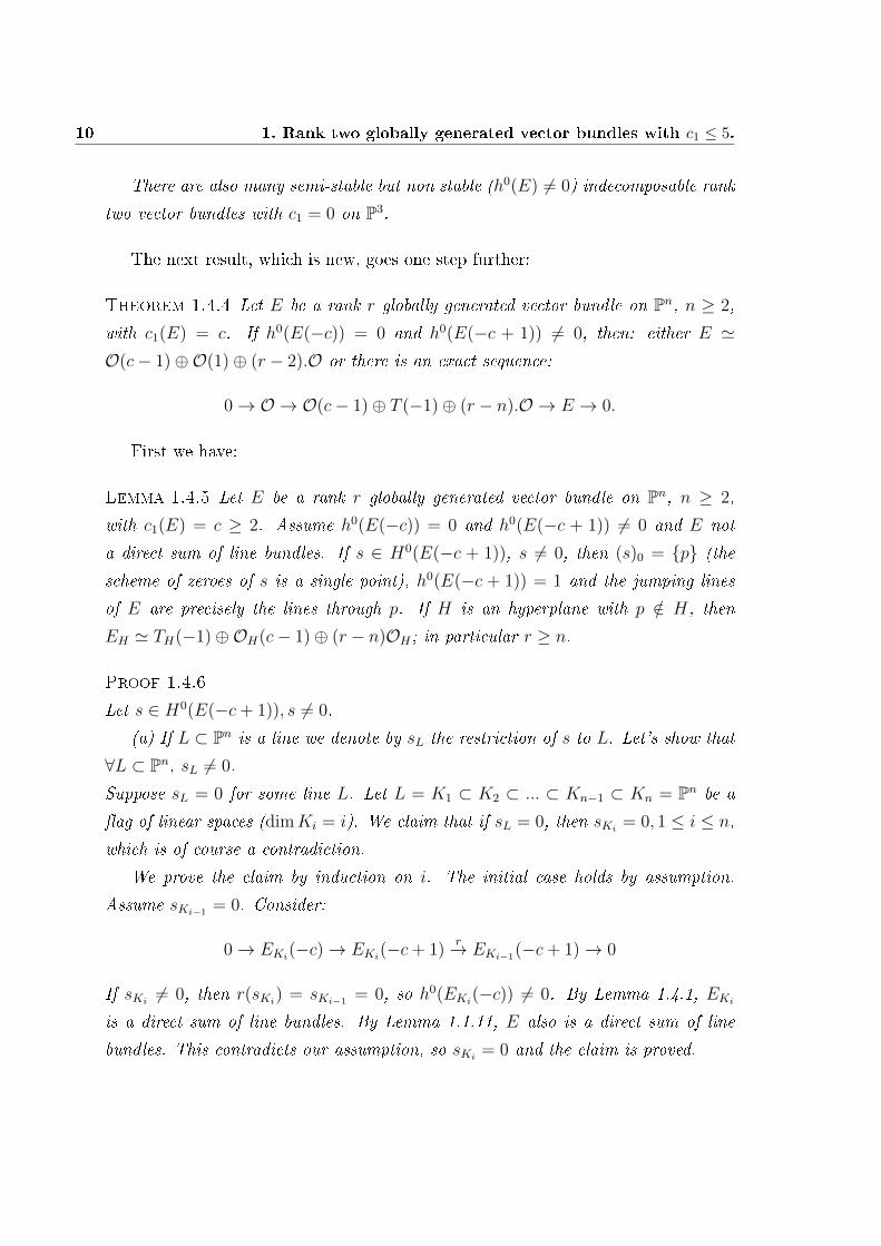
Theorem 1.4.4 Let E be a rank r globally generated vector bundle on Pn, n ≥ 2,
with c1(E) = c. If h0(E(−c)) = 0 and h0(E(−c + 1)) 6= 0, then: either E 'O(c− 1)⊕O(1)⊕ (r − 2).O or there is an exact sequence:
0→ O → O(c− 1)⊕ T (−1)⊕ (r − n).O → E → 0.
First we have:
Lemma 1.4.5 Let E be a rank r globally generated vector bundle on Pn, n ≥ 2,
with c1(E) = c ≥ 2. Assume h0(E(−c)) = 0 and h0(E(−c + 1)) 6= 0 and E not
a direct sum of line bundles. If s ∈ H0(E(−c + 1)), s 6= 0, then (s)0 = p (the
scheme of zeroes of s is a single point), h0(E(−c + 1)) = 1 and the jumping lines
of E are precisely the lines through p. If H is an hyperplane with p /∈ H, then
EH ' TH(−1)⊕OH(c− 1)⊕ (r − n)OH ; in particular r ≥ n.
Proof 1.4.6
Let s ∈ H0(E(−c+ 1)), s 6= 0.
(a) If L ⊂ Pn is a line we denote by sL the restriction of s to L. Let's show that
∀L ⊂ Pn, sL 6= 0.
Suppose sL = 0 for some line L. Let L = K1 ⊂ K2 ⊂ ... ⊂ Kn−1 ⊂ Kn = Pn be a
ag of linear spaces (dimKi = i). We claim that if sL = 0, then sKi= 0, 1 ≤ i ≤ n,
which is of course a contradiction.
We prove the claim by induction on i. The initial case holds by assumption.
Assume sKi−1= 0. Consider:
0→ EKi(−c)→ EKi
(−c+ 1)r→ EKi−1
(−c+ 1)→ 0
If sKi6= 0, then r(sKi
) = sKi−1= 0, so h0(EKi
(−c)) 6= 0. By Lemma 1.4.1, EKi
is a direct sum of line bundles. By Lemma 1.1.11, E also is a direct sum of line
bundles. This contradicts our assumption, so sKi= 0 and the claim is proved.
1.4 A general result. 11
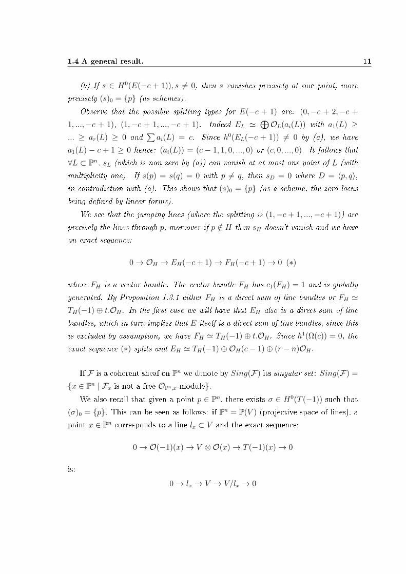
(b) If s ∈ H0(E(−c + 1)), s 6= 0, then s vanishes precisely at one point, more
precisely (s)0 = p (as schemes).
Observe that the possible splitting types for E(−c + 1) are: (0,−c + 2,−c +
1, ...,−c + 1), (1,−c + 1, ...,−c + 1). Indeed EL '⊕OL(ai(L)) with a1(L) ≥
... ≥ ar(L) ≥ 0 and∑ai(L) = c. Since h0(EL(−c + 1)) 6= 0 by (a), we have
a1(L) − c + 1 ≥ 0 hence: (ai(L)) = (c − 1, 1, 0, ..., 0) or (c, 0, ..., 0). It follows that
∀L ⊂ Pn, sL (which is non zero by (a)) can vanish at at most one point of L (with
multiplicity one). If s(p) = s(q) = 0 with p 6= q, then sD = 0 where D = 〈p, q〉,in contradiction with (a). This shows that (s)0 = p (as a scheme, the zero locus
being dened by linear forms).
We see that the jumping lines (where the splitting is (1,−c + 1, ...,−c + 1)) are
precisely the lines through p, moreover if p /∈ H then sH doesn't vanish and we have
an exact sequence:
0→ OH → EH(−c+ 1)→ FH(−c+ 1)→ 0 (∗)
where FH is a vector bundle. The vector bundle FH has c1(FH) = 1 and is globally
generated. By Proposition 1.3.1 either FH is a direct sum of line bundles or FH 'TH(−1) ⊕ t.OH . In the rst case we will have that EH also is a direct sum of line
bundles, which in turn implies that E itself is a direct sum of line bundles, since this
is excluded by assumption, we have FH ' TH(−1)⊕ t.OH . Since h1(Ω(c)) = 0, the
exact sequence (∗) splits and EH ' TH(−1)⊕OH(c− 1)⊕ (r − n)OH .
If F is a coherent sheaf on Pn we denote by Sing(F) its singular set : Sing(F) =
x ∈ Pn | Fx is not a free OPn,x-module.We also recall that given a point p ∈ Pn, there exists σ ∈ H0(T (−1)) such that
(σ)0 = p. This can be seen as follows: if Pn = P(V ) (projective space of lines), a
point x ∈ Pn corresponds to a line lx ⊂ V and the exact sequence:
0→ O(−1)(x)→ V ⊗O(x)→ T (−1)(x)→ 0
is:
0→ lx → V → V/lx → 0

12 1. Rank two globally generated vector bundles with c1 ≤ 5.
so that we may identify the (vector bundle) ber T (−1)(x) := T (−1) ⊗ k(x) with
V/lx. With this identication any v ∈ V yields a section, sv, of T (−1) with sv(x) =
v ∈ V/lx. Clearly sv(x) = 0⇔ lx = 〈v〉.
Lemma 1.4.7 Let G be a rank n − 1, globally generated torsion free sheaf on Pn,n ≥ 2, with Sing(G) = p, c1(G) = 1 and h0(G) = n. If n = 2 then G ' Ip(1); if
n > 2, G is reexive. In any case there is an exact sequence:
0→ O → T (−1)→ G → 0
Proof 1.4.8
Since G is globally generated with h0(G) = n there is an exact sequence:
0→ L → n.O → G → 0
Since G is torsion free and n.O is reexive, L is normal ([18], Chap. II, Lemma
1.1.16). Since L is torsion free and normal, L is reexive ([18], Chap. II, Lemma
1.1.12). Finally since L has rank one and is reexive, it is locally free ([18], Chap.
II, Lemma 1.1.15). Looking at Chern classes we get that L ' O(−1). In conclusion
we have:
0→ O(−1)f→ n.O → G → 0 (+)
The map f is given by n linear forms ϕ1, ..., ϕn. Since Sing(G) = p, ϕ1, ..., ϕn are
linearly independent and dene the point p.
If n = 2 we clearly have G ' Ip(1); moreover if n > 2, G is reexive (just take
the bidual of (+) and take into account that Ext1(O, Ip) = 0 if n > 2).
After a change of coordinates we may assume p = (1 : 0 : ... : 0) and f given by
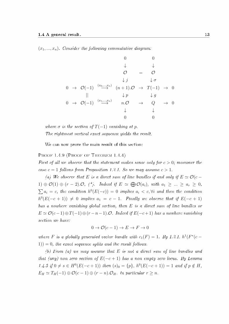
1.4 A general result. 13
(x1, ..., xn). Consider the following commutative diagram:
0 0
↓ ↓O = O↓ j ↓ σ
0 → O(−1)(x0,...,xn)−→ (n+ 1).O → T (−1) → 0
|| ↓ p ↓ g0 → O(−1)
(x1,...,xn)−→ n.O → Q → 0
↓ ↓0 0
where σ is the section of T (−1) vanishing at p.
The rightmost vertical exact sequence yields the result.
We can now prove the main result of this section:
Proof 1.4.9 (Proof of Theorem 1.4.4)
First of all we observe that the statement makes sense only for c > 0; moreover the
case c = 1 follows from Proposition 1.3.1. So we may assume c > 1.
(a) We observe that E is a direct sum of line bundles if and only if E ' O(c−1) ⊕ O(1) ⊕ (r − 2).O, (*). Indeed if E ' ⊕O(ai), with a1 ≥ ... ≥ ar ≥ 0,∑ai = c, the condition h0(E(−c)) = 0 implies ai < c,∀i and then the condition
h0(E(−c + 1)) 6= 0 implies a1 = c − 1. Finally we observe that if E(−c + 1)
has a nowhere vanishing global section, then E is a direct sum of line bundles or
E ' O(c−1)⊕T (−1)⊕ (r−n−1).O. Indeed if E(−c+1) has a nowhere vanishing
section we have:
0→ O(c− 1)→ E → F → 0
where F is a globally generated vector bundle with c1(F ) = 1. By 1.3.1, h1(F ∗(c −1)) = 0, the exact sequence splits and the result follows.
(b) From (a) we may assume that E is not a direct sum of line bundles and
that (any) non zero section of E(−c + 1) has a non empty zero locus. By Lemma
1.4.5 if 0 6= s ∈ H0(E(−c + 1)) then (s)0 = p, h0(E(−c + 1)) = 1 and if p /∈ H,
EH ' TH(−1)⊕O(c− 1)⊕ (r − n).OH . In particular r ≥ n.
14 1. Rank two globally generated vector bundles with c1 ≤ 5.
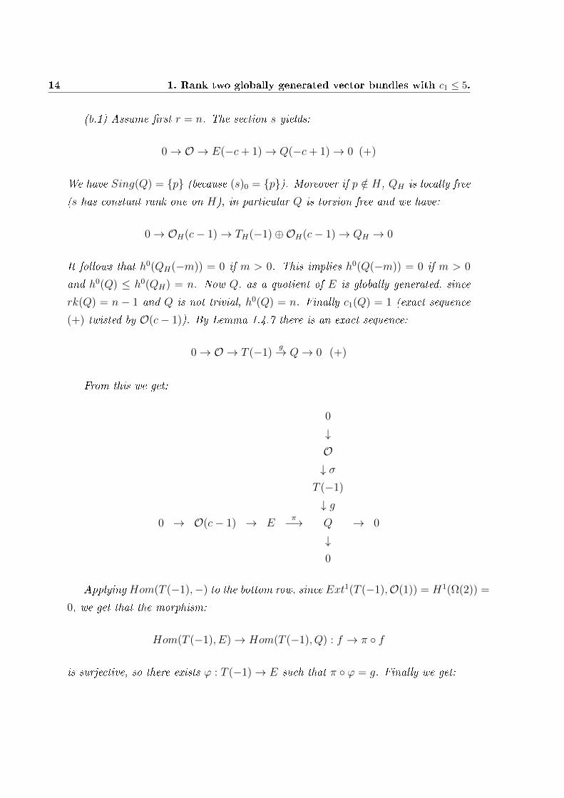
(b.1) Assume rst r = n. The section s yields:
0→ O → E(−c+ 1)→ Q(−c+ 1)→ 0 (+)
We have Sing(Q) = p (because (s)0 = p). Moreover if p /∈ H, QH is locally free
(s has constant rank one on H), in particular Q is torsion free and we have:
0→ OH(c− 1)→ TH(−1)⊕OH(c− 1)→ QH → 0
It follows that h0(QH(−m)) = 0 if m > 0. This implies h0(Q(−m)) = 0 if m > 0
and h0(Q) ≤ h0(QH) = n. Now Q, as a quotient of E is globally generated, since
rk(Q) = n − 1 and Q is not trivial, h0(Q) = n. Finally c1(Q) = 1 (exact sequence
(+) twisted by O(c− 1)). By Lemma 1.4.7 there is an exact sequence:
0→ O → T (−1)g→ Q→ 0 (+)
From this we get:
0
↓O↓ σ
T (−1)
↓ g0 → O(c− 1) → E
π−→ Q → 0
↓0
Applying Hom(T (−1),−) to the bottom row, since Ext1(T (−1),O(1)) = H1(Ω(2)) =
0, we get that the morphism:
Hom(T (−1), E)→ Hom(T (−1), Q) : f → π f
is surjective, so there exists ϕ : T (−1)→ E such that π ϕ = g. Finally we get:

1.4 A general result. 15
0 0
↓ ↓O = O↓ ↓ σ
0 → O(c− 1)s−→ O(c− 1)⊕ T (−1) → T (−1) → 0
|| ↓ (s, ϕ) ↓ g0 → O(c− 1)
s−→ E → Q → 0
↓ ↓0 0
In conclusion:
0→ O → O(c− 1)⊕ T (−1)→ E → 0
(b.2) Assume now r > n.
By Lemma 1.1.4 we have an exact sequence:
0→ (r − n).O → E → E → 0
where E is a rank n, globally generated vector bundle with h0(E(−t)) = h0(E(−t)),∀t >0 and c1(E) = c1(E). If E is a direct sum of line bundles, then E also is, in contrast
with our assumption. So E is as in (b.1), i.e there is an exact sequence:
0→ O → O(c− 1)⊕ T (−1)→ E → 0
We have:
0
↓O↓
O(c− 1)⊕ T (−1)
↓ g0 → (r − n).O → E
π−→ E → 0
↓0

16 1. Rank two globally generated vector bundles with c1 ≤ 5.
Applying Hom(O(c− 1)⊕ T (−1),−) to the bottom row, since Ext1(O(c− 1)⊕T (−1),O) = H1(Ω(1)⊕O(−c+ 1)) = 0, we get that the morphism:
Hom(O(c− 1)⊕ T (−1), E)→ Hom(O(c− 1)⊕ T (−1), Q) : f → π f
is surjective, so there exists ϕ : O(c− 1)⊕ T (−1)→ E such that π ϕ = g. Finally
we get:
0→ O → O(c− 1)⊕ T (−1)⊕ (r − n).O → E → 0
and the proof is over.
1.5 Globally generated vector bundles on Pn with
c1 = 2.
The classication of globally generated vector bundles on Pn with c1 = 2 has been
achieved recently by Sierra-Ugaglia ([21]). Their result is:
Theorem 1.5.1 Let E be a globally generated, rank r, vector bundle on Pn, n ≥ 2,
with c1 = 2, then one of the following holds:
1. E ' O(2)⊕ (r − 1).O
2. E ' 2.O(1)⊕ (r − 2).O
3. there is an exact sequence:
0→ O → O(1)⊕ T (−1)⊕ (r − n).O → E → 0
4. there is an exact sequence:
0→ 2.O(−1)→ (r + 2).O → E → 0
5. there is an exact sequence:
0→ O(−2)→ (r + 1).O → E → 0
1.5 Globally generated vector bundles on Pn with c1 = 2. 17
6. n = 3 and E ' Ω(2)⊕ (r − 3).O
7. n = 3 and E ' N (1) ⊕ (r − 2).O, where N is a normalized null-correlation
bundle.
As we can see the number of possibilities increases and also some exceptional
cases appear (for n = 3). We observe that h0(E(−2)) 6= 0 in case (1), h0(E(−2)) = 0
but h0(E(−1)) 6= 0 in cases (2), (3) and h0(E(−1)) = 0 in the remaining cases.
Let's sketch the proof of the theorem.
Lemma 1.5.2 Let E be a rank r globally generated vector bundle on Pn, n ≥ 2 with
c1 = 2. If h0(E(−1)) 6= 0, then one of the cases (1), (2), (3) of Theorem 1.5.1
occurs.
Proof 1.5.3
Follows from Lemma 1.4.1 and Theorem 1.4.4.
From now on we may assume h0(E(−1)) = 0. Let's prove the Theorem for n = 2:
Lemma 1.5.4 Let E be a rank r globally generated vector bundle on P2 with c1 = 2.
If h0(E(−1)) = 0 then one of the following occurs:
1.
0→ O(−2)→ (r + 1).O → E → 0
2.
0→ 2.O(−1)→ (r + 2).O → E → 0
Proof 1.5.5
Let L ⊂ P2 be a line, the exact sequence:
0→ E(−1)→ E → EL → 0
shows, since h0(E(−1)) = 0, that h0(E) ≤ h0(EL) = r+2. So r+1 ≤ h0(E) ≤ r+2
and if h0(E) = r + 1, we are in case (1). If h0(E) = r + 2, we have:
0→ E → (r + 2).O → E → 0
18 1. Rank two globally generated vector bundles with c1 ≤ 5.
where E has rank two and c1 = −2. We have h1(E(−m)) = 0 if m ≥ 0. Since
h1(E(m)) = h1(E∗(−m− 3)) = h1(E(−m− 1)), we conclude that H1∗ (E) = 0 and (by
Theorem 1.1.10), E is a direct sum of line bundles. Since E∗ is globally generated
and h0(E) = r + 2 we get E ' 2.O(−1).
So far the Theorem is proved for n = 2. The following lemma shows that the
case n = 3 is special.
Lemma 1.5.6 Let E be a globally generated rank r vector bundle on Pn, n ≥ 3, with
c1(E) = 2. If h0(E(−1)) = 0 but h0(EH(−1)) 6= 0 for some hyperplane H, then
n = 3.
Proof 1.5.7
If EH is a direct sum of line bundles, then E also is a direct sum of line bundles,
but this is impossible since h0(E(−1)) = 0. By 1.4.4 we conclude that:
0→ OH → TH(−1)⊕OH(1)⊕ (r − n+ 1).OH → EH → 0
In particular r ≥ n − 1. If n > 3, hi(EH(−m)) = 0 for i = 0, 1 and m ≥ 2. It
follows that h0(E(−2)) = h1(E(−2)) = 0. From the exact sequence:
0→ E(−2)→ E(−1)→ EH(−1)→ 0
we get h0(E(−1)) = h0(EH(−1)) > 0: a contradiction if n > 3, hence n = 3.
Proposition 1.5.8 Let E be a globally generated vector bundle of rank r on P3
with c1(E) = 2. Assume h0(E(−1)) = 0 but h0(EH(−1)) 6= 0 for some hyperplane.
Then:
E ' Ω(2)⊕ (r − 3).O or E ' N (1)⊕ (r − 2).O
where N is a normalized null-correlation bundle.
Proof 1.5.9
We have
0→ OH → TH(−1)⊕OH(1)⊕ (r − n+ 1).OH → EH → 0 (+)
1.5 Globally generated vector bundles on Pn with c1 = 2. 19
In particular r ≥ 2, c1(E) = c2(E) = 2.
(a) If r = 2, E(−1) is stable with c1 = 0, c2 = 1, hence E(−1) is a null-
correlation bundle. This can be seen also as follows: a general section yields: 0 →O → E → IC(2) → 0, where C is a smooth curve with ωC(2) ' OC. It follows
that C is a disjoint union of lines. Since IC(2) is globally generated, C has degree
≤ 2; it can't be 1 because E doesn't split, so C is the union of two skew lines (or
deg(C) = c2(E) = 2) and E = N (1).
(b) Assume r = 3. We have h0(E) ≤ h0(EH) = 6. By Riemann-Roch, since
c1 = c2 = 2, χ(E) = c32
+ 6. Using the dual of (+) we have hi(E∗H(−m)) = 0 if
m ≥ 4, i = 0, 1. From 0 → E∗(−m − 1) → E∗(−m) → E∗H(−m) → 0, we get
h1(E∗(−4)) = h2(E) = 0. So χ(E) = h0(E) − h1(E) − h3(E) = c32
+ 6. Since
h0(E) ≤ 6 and c3 ≥ 0 (because E is globally generated), it follows that c3 = 0. This
implies (??) that a general section of E doesn't vanish, hence we have:
0→ O → E → F → 0
where F is a rank two globally generated vector bundle with c1(F ) = 2. Since
h0(F (−1)) = 0 and h0(FH(−1)) 6= 0, F ' N (1). We have dimExt1(O,N (1)) =
h1(N ∗(−1)) = 1 and it is well known that there are two extensions: the trivial one
and
0→ O → Ω(2)→ N (1)→ 0
We conclude that E ' Ω(2) or E ' N (1)⊕O.(c) Finally if r > 3 there is an exact sequence:
0→ (r − 3).O → E → E → 0
where E is globally generated of rank three, with c1(E) = 2, h0(E(−1)) = 0 and
h0(EH(−1)) 6= 0. Then E is as in (b) and we easily conclude that E ' Ω(2)⊕(r−3).Oor E ' N (1)⊕ (r − 2).O.
We can now conclude the proof of the Theorem for n = 3:
Lemma 1.5.10 Let E be a globally generated vector bundle of rank r on P3 with
c1 = 2. If h0(E(−1)) = 0 and h0(EH(−1)) = 0 for all (some) hyperplane, then
20 1. Rank two globally generated vector bundles with c1 ≤ 5.
either:
0→ O(−2)→ (r + 1).O → E → 0
or
0→ 2.O(−1)→ (r + 2).O → E → 0
Proof 1.5.11
Since h0(E(−1)) = h0(EH(−1)) = 0, we have h0(E) ≤ h0(EH) ≤ h0(EL) = r+2. If
h0(E) = r + 1 we are in the rst case. If h0(E) = r + 2 there is an exact sequence:
0→ E → (r + 2).O → E → 0
restricting to H we get (see 1.5.4) E ' 2.O(−1).
The nal touch:
Proof 1.5.12 (Proof of theorem 1.5.1)
According to the previous results we may assume n ≥ 4 and h0(E(−1)) = 0. By
Lemma 1.5.6, h0(EH(−1)) = 0 for some (in fact all) hyperplane. Let's prove by
induction on n that under these assumptions either case (4) or case (5) of 1.5.1
holds.
Assume rst n = 4. From Proposition 1.5.8 and Lemma 1.5.10, either h0(EH) ≤r + 2 or EH ' ΩH(2)⊕ (r− 3)OH or EH ' N (1)⊕ (r− 2).OH . The last two cases
are impossible. Indeed there is no globally generated vector bundle E on P4 with
EH ' ΩH(2)⊕ (r − 3).OH or N (1)⊕ (r − 2).OH : such a vector bundle would have
c1 = c2 = 2 and c3(E) = 0; r−2 general sections would give a morphism of constant
rank (because c3 = 0) hence a rank two vector bundle as quotient with c1 = c2 = 2,
but this contradicts Schwarzenberger's conditions. So h0(EH) ≤ r + 2, hence, since
h0(E(−1)) = 0, h0(E) ≤ r + 2 and we easily conclude (see proof of 1.5.10).
Assume the result for n− 1. In particular this means h0(EH) ≤ r+ 2. It follows
that h0(E) ≤ r + 2 and we are home.

1.6 Globally generated rank two vector bundles on Pn, n ≥ 3, with c1 ≤ 5. 21
1.6 Globally generated rank two vector bundles on
Pn, n ≥ 3, with c1 ≤ 5.
In this section we consider rank two globally generated vector bundles on Pn with
c1 ≤ 5. The nal result is:
Theorem 1.6.1 Let E be a rank two vector bundle on Pn, n ≥ 3, generated by
global sections with Chern classes c1, c2, c1 ≤ 5.
1. If n ≥ 4, then E is the direct sum of two line bundles
2. If n = 3 and E is indecomposable, then
(c1, c2) ∈ S = ((2, 2), (4, 5), (4, 6), (4, 7), (4, 8), (5, 8), (5, 10), (5, 12).
If E exists there is an exact sequence: 0 → O → E → IC(c1) → 0 (∗), whereC ⊂ P3 is a smooth curve of degree c2 with ωC(4− c1) ' OC. The curve C is
irreducible, except maybe if (c1, c2) = (4, 8): in this case C can be irreducible
or the disjoint union of two smooth conics.
3. For every (c1, c2) ∈ S, (c1, c2) 6= (5, 12), there exists a rank two vector bundle
on P3 with Chern classes (c1, c2) which is globally generated (and with an exact
sequence as in (2)).
Remark 1.6.2 The case n = 3, (c1, c2) = (5, 12) remains open: we are unable to
prove or disprove the existence of such bundles.
1.6.1 Globally generated rank two vector bundles on P3 with
c1 = 3.
The following result has been proved in [22] (with a dierent and longer proof).
Proposition 1.6.3 Let E be a rank two globally generated vector bundle on P3. If
c1(E) = 3 then E splits.

22 1. Rank two globally generated vector bundles with c1 ≤ 5.
Proof 1.6.4 Assume a general section vanishes in codimension two, then it van-
ishes along a smooth curve C such that ωC ' OC(−1). Moreover IC(3) is generated
by global sections. We have C = ∪ri=1Ci (disjoint union) where each Ci is smooth
irreducible with ωCi' OCi
(−1). It follows that each Ci is a smooth conic. If r ≥ 2
let L = 〈C1〉 ∩ 〈C2〉 (〈Ci〉 is the plane spanned by Ci). Every cubic containing C
contains L (because it contains the four points C1∩L, C2∩L). This contradicts thefact that IC(3) is globally generated. Hence r = 1 and E = O(1)⊕O(2).
1.6.2 Globally generated rank two vector bundles on P3 with
c1 = 4.
Let's start with a general result:
Lemma 1.6.5 Let E be a non split rank two vector bundle on P3 with Chern classes
c1, c2. If E is globally generated and if c1 ≥ 4 then:
c2 ≤2c3
1 − 4c21 + 2
3c1 − 4.
Proof 1.6.6 By our assumptions a general section of E vanishes along a smooth
curve, C, such that IC(c1) is generated by global sections. Let U be the complete
intersections of two general surfaces containing C. Then U links C to a smooth
curve, Y . We have Y 6= ∅ since E doesn't split. The exact sequence of liaison:
0→ IU(c1)→ IC(c1)→ ωY (4− c1)→ 0 shows that ωY (4− c1) is generated by global
sections. Hence deg(ωY (4− c1)) ≥ 0. We have deg(ωY (4− c1)) = 2g′−2 +d′(4− c1)
(g′ = pa(Y ), d′ = deg(Y )). So g′ ≥ d′(c1−4)+22
≥ 0 (because c1 ≥ 4). On the
other hand, always by liaison, we have: g′ − g = 12(d′ − d)(2c1 − 4) (g = pa(C),
d = deg(C)). Since d′ = c21 − d and g = d(c1−4)
2+ 1 (because ωC(4− c1) ' OC), we
get: g′ = 1 + d(c1−4)2
+ 12(c2
1 − 2d)(2c1 − 4) ≥ 0 and the result follows.
Now we have:
Proposition 1.6.7 Let E be a rank two globally generated vector bundle on P3. If
c1(E) = 4 and if E doesn't split, then 5 ≤ c2 ≤ 8 and there is an exact sequence:
1.6 Globally generated rank two vector bundles on Pn, n ≥ 3, with c1 ≤ 5. 23
0→ O → E → IC(4)→ 0, where C is a smooth irreducible elliptic curve of degree
c2 or, if c2 = 8, C is the disjoint union of two smooth elliptic quartic curves.
Proof 1.6.8 A general section of E vanishes along C where C is a smooth curve
with ωC = OC and where IC(4) is generated by global sections. Let C = C1∪ ...∪Crbe the decomposition into irreducible components: the union is disjoint, each Ci is a
smooth elliptic curve hence has degree at least three.
By Lemma 1.6.5 d = deg(C) ≤ 8. If d ≤ 4 then C is irreducible and is a complete
intersection which is impossible since E doesn't split. If d = 5, C is smooth irre-
ducible.
Claim: If 8 ≥ d ≥ 6, C cannot contain a plane cubic curve.
Assume C = P ∪X where P is a plane cubic and where X is a smooth elliptic curve
of degree d − 3. If d = 6, X is also a plane cubic and every quartic containing C
contains the line 〈P 〉 ∩ 〈X〉. If deg(X) ≥ 4 then every quartic, F , containing C
contains the plane 〈P 〉. Indeed F |H vanishes on P and on the deg(X) ≥ 4 points
of X ∩ 〈P 〉, but these points are not on a line so F |H = 0. In both cases we get a
contradiction with the fact that IC(4) is generated by global sections. The claim is
proved.
It follows that, if 8 ≥ d ≥ 6, then C is irreducible except if C = X∪Y is the disjoint
union of two elliptic quartic curves.
Now let's show that all possibilities of Proposition 1.6.7 do actually occur. For
this we have to show the existence of a smooth irreducible elliptic curve of degree d,
5 ≤ d ≤ 8 with IC(4) generated by global sections (and also that the disjoint union
of two elliptic quartc curves is cut o by quartics).
Lemma 1.6.9 There exist rank two vector bundles with c1 = 4, c2 = 5 which are
globally generated. More precisely any such bundle is of the form N (2), where N is
a null-correlation bundle (a stable bundle with c1 = 0, c2 = 1).
Proof 1.6.10 The existence is clear (if N is a null-correlation bundle then it is well
known that N (k) is globally generated if k ≥ 1). Conversely if E has c1 = 4, c2 = 5
and is globally generated, then E has a section vanishing along a smooth, irreducible
quintic elliptic curve (cf 1.6.7). Since h0(IC(2)) = 0, E is stable, hence E = N (2).

24 1. Rank two globally generated vector bundles with c1 ≤ 5.
Lemma 1.6.11 There exist smooth, irreducible elliptic curves, C, of degree 6 with
IC(4) generated by global sections.
Proof 1.6.12 Let X be the union of three skew lines. The curve X lies on a smooth
quadric surface, Q, and has IX(3) globally generated (indeed the exact sequence
0 → IQ → IX → IX,Q → 0 twisted by O(3) reads like: 0 → O(1) → IC(3) →OQ(3, 0) → 0). The complete intersection, U , of two general cubics containing
X links X to a smooth curve, C, of degree 6 and arithmetic genus 1. Since, by
liaison, h1(IC) = h1(IX(−2)) = 0, C is irreducible. The exact sequence of liaison:
0→ IU(4)→ IC(4)→ ωX(2)→ 0 shows that IC(4) is globally generated.
In order to prove the existence of smooth, irreducible elliptic curves, C, of degree
d = 7, 8, with IC(4) globally generated, we have to recall some results due to Mori
([16]).
According to [16] Remark 4, Prop. 6, there exists a smooth quartic surface
S ⊂ P3 such that Pic(S) = ZH ⊕ ZX where X is a smooth elliptic curve of degree
d (7 ≤ d ≤ 8). The intersection pairing is given by: H2 = 4, X2 = 0, H.X = d.
Such a surface doesn't contain any smooth rational curve ([16] p.130). In particular:
(∗) every integral curve, Z, on S has degree ≥ 4 with equality if and only if Z is a
planar quartic curve or an elliptic quartic curve.
Lemma 1.6.13 With notations as above, h0(IX(3)) = 0.
Proof 1.6.14 A curve Z ∈ |3H −X| has invariants (dZ , gZ) = (5,−2) (if d = 7)
or (4,−5) (if d = 8), so Z is not integral. It follows that Z must contain an integral
curve of degree < 4, but this is impossible.
Lemma 1.6.15 With notations as above |4H − X| is base point free, hence there
exist smooth, irreducible elliptic curves, X, of degree d, 7 ≤ d ≤ 8, such that IX(4)
is globally generated.
Proof 1.6.16 Let's rst prove the following: Claim: Every curve in |4H − X| isintegral.

1.6 Globally generated rank two vector bundles on Pn, n ≥ 3, with c1 ≤ 5. 25
If Y ∈ |4H − X| is not integral then Y = Y1 + Y2 where Y1 is integral with
deg(Y1) = 4 (observe that deg(Y ) = 9 or 8).
If Y1 is planar then Y1 ∼ H, so 4H−X ∼ H+Y2 and it follows that 3H ∼ X+Y2,
in contradiction with h0(IX(3)) = 0 (cf 1.6.13).
So we may assume that Y1 is a quartic elliptic curve, i.e. (i) Y 21 = 0 and (ii)
Y1.H = 4. Setting Y1 = aH+bX, we get from (i): 2a(2a+bd) = 0. Hence (α) a = 0,
or (β) 2a+ bd = 0.
(α) In this case Y1 = bX, hence (for degree reasons and since S doesn't contain
curves of degree < 4), Y2 = ∅ and Y = X, which is integral.
(β) Since Y1.H = 4, we get 2a + (2a + bd) = 2a = 4, hence a = 2 and bd = −4
which is impossible (d = 7 or 8 and b ∈ Z).This concludes the proof of the claim.
Since (4H − X)2 ≥ 0, the claim implies that 4H − X is numerically eective.
Now we conclude by a result of Saint-Donat (cf [16], Theorem 5) that |4H −X| isbase point free, i.e. IX,S(4) is globally generated. By the exact sequence: 0→ O →IX(4)→ IX,S(4)→ 0 we get that IX(4) is globally generated.
Remark 1.6.17 If d = 8, a general element Y ∈ |4H − X| is a smooth elliptic
curve of degree 8. By the way Y 6= X (see [2]). The exact sequence of liaison:
0 → IU(4) → IX(4) → ωY → 0 shows that h0(IX(4)) = 3 (i.e. X is of maximal
rank). In case d = 8 Lemma 1.6.15 is stated in [5], however the proof there is
incomplete, indeed in order to apply the enumerative formula of [12] one has to
know that X is a connected component of3⋂i=1
Fi; this amounts to say that the base
locus of |4H −X| on F1 has dimension ≤ 0.
To conclude we have:
Lemma 1.6.18 Let X be the disjoint union of two smooth, irreducible quartic elliptic
cuvres, then IX(4) is generated by global sections.
Proof 1.6.19 Let X = C1 t C2. We have: 0 → O(−4) → 2.O(−2) → IC1 → 0,
twisting by IC2, since C1 ∩ C2 = ∅, we get:
0→ IC2(−4)→ 2.IC2(−2)→ IX → 0 and the result follows.
26 1. Rank two globally generated vector bundles with c1 ≤ 5.
Summarizing:
Proposition 1.6.20 There exists an indecomposable rank two vector bundle, E,
on P3, generated by global sections and with c1(E) = 4 if and only if 5 ≤ c2(E) ≤ 8
and in these cases there is an exact sequence:
0→ O → E → IC(4)→ 0
where C is a smooth irreducible elliptic curve of degree c2(E) or, if c2(E) = 8, the
disjoint union of two smooth elliptic quartic curves.
1.6.3 Globally generated rank two vector bundles on P3 with
c1 = 5.
We start by listing the possible cases:
Proposition 1.6.21 If E is an indecomposable, globally generated, rank two vector
bundle on P3 with c1(E) = 5, then c2(E) ∈ 8, 10, 12 and there is an exact sequence:
0→ O → E → IC(5)→ 0
where C is a smooth, irreducible curve of degree d = c2(E), with ωC ' OC(1).
In any case E is stable.
Proof 1.6.22 A general section of E vanishes along a smooth curve, C, of degree
d = c2(E) with ωC ' OC(1). Hence every irreducible component, Y , of C is a
smooth, irreducible curve with ωY ' OY (1). In particular deg(Y ) = 2g(Y ) − 2 is
even and deg(Y ) ≥ 4.
1. If d = 4, then C is a planar curve and E splits.
2. If d = 6, C is necessarily irreducible (of genus 4). It is well known that any
such curve is a complete intersection (2, 3), hence E splits.

1.6 Globally generated rank two vector bundles on Pn, n ≥ 3, with c1 ≤ 5. 27
3. If d = 8 and C is not irreducible, then C = P1 t P2, the disjoint union of
two planar quartic curves. If L = 〈P1〉 ∩ 〈P2〉, then every quintic containing
C contains L in contradiction with the fact that IC(5) is generated by global
sections. Hence C is irreducible.
4. If d = 10 and C is not irreducible, then C = P tX, where P is a planar curve
of degree 4 and where X is a degree 6 curve (X is a complete intersection
(2, 3)). Every quintic containing C vanishes on P and on the 8 points of
X ∩ 〈P 〉, since these 8 points are not on a line, the quintic vanishes on the
plane 〈P 〉. This contradicts the fact that IC(5) is globally generated.
5. If d = 12 and C is not irreducible we have three possibilities:
(a) C = P1 t P2 t P3, Pi planar quartic curves
(b) C = X1 tX2, Xi complete intersection curves of types (2, 3)
(c) C = Y t P , Y a canonical curve of degree 8, P a planar curve of degree
4.
(a) This case is impossible (consider the line 〈P1〉 ∩ 〈P2〉).(b) We have Xi = Qi∩Fi. Let Z be the quartic curve Q1∩Q2. Then Xi∩Z =
Fi∩Z, i.e. Xi meets Z in 12 points. It follows that every quintic containing C
meets Z in 24 points, hence such a quintic contains Z. Again this contradicts
the fact that IC(5) is globally generated.
(c) This case too is impossible: every quintic containing C vanishes on P and
on the points 〈P 〉 ∩ Y , hence on 〈P 〉.
We conclude that if d = 12, C is irreducible.
The normalized bundle is E(−3), since in any case h0(IC(2)) = 0 (every smooth
irreducible subcanonical curve on a quadric surface is a complete intersection), E is
stable.
Now we turn to the existence part.
Lemma 1.6.23 There exist indecomposable rank two vector bundles on P3 with Chern
classes c1 = 5 and c2 ∈ 8, 10 which are globally generated.
28 1. Rank two globally generated vector bundles with c1 ≤ 5.
Proof 1.6.24 Let R = tsi=1Li be the union of s disjoint lines, 2 ≤ s ≤ 3. We may
perform a liaison (s, 3) and link R to K = tsi=1Ki, the union of s disjoint conics.
The exact sequence of liaison: 0 → IU(4) → IK(4) → ωR(5 − s) → 0 shows that
IK(4) is globally generated (n.b. 5− s ≥ 2).
Since ωK(1) ' OK we have an exact sequence: 0→ O → E(2)→ IK(3)→ 0, where
E is a rank two vector bundle with Chern classes c1 = −1, c2 = 2s− 2. Twisting by
O(1) we get: 0 → O(1) → E(3) → IK(4) → 0 (∗). The Chern classes of E(3) are
c1 = 5, c2 = 2s + 4 (i.e. c2 = 8, 10). Since IK(4) is globally generated, it follows
from (∗) that E(3) too, is generated by global sections.
Remark 1.6.25
1. If E is as in the proof of Lemma 1.6.23 a general section of E(3) vanishes along
a smooth, irreducible (because h1(E(−2)) = 0) canonical curve, C, of genus
1+ c2/2 (g = 5, 6) such that IC(5) is globally generated. By construction these
curves are not of maximal rank (h0(IC(3)) = 1 if g = 5, h0(IC(4)) = 2 if
g = 6). As explained in [13] o4 this is a general fact: no canonical curve of
genus g, 5 ≤ g ≤ 6 in P3 is of maximal rank. We don't know if this is still true
for g = 7.
2. According to [13] the general canonical curve of genus 6 lies on a unique quartic
surface.
3. The proof of 1.6.23 breaks down with four conics: IK(4) is no longer globally
generated, every quartic containing K vanishes along the lines Li (5− s = 1).
Observe also that four disjoint lines always have a quadrisecant and hence are
an exception to the normal generation conjecture(the omogeneous ideal is not
generated in degree three as it should be).
Remark 1.6.26 The case (c1, c2) = (5, 12) remains open. It can be shown that if
E exists, a general section of E is linked, by a complete intersections of two quintics,
to a smooth, irreducible curve, X, of degree 13, genus 10 having ωX(−1) as a base
point free g15. One can prove the existence of curves X ⊂ P3, smooth, irreducible, of
degree 13, genus 10, with ωX(−1) a base point free pencil and lying on one quintic
1.6 Globally generated rank two vector bundles on Pn, n ≥ 3, with c1 ≤ 5. 29
surface. But we are unable to show the existence of such a curve with h0(IX(5)) ≥ 2
(which will imply the existence of our vector bundle).
1.6.4 Globally generated rank two vector bundles on Pn, n ≥ 4
with c1 ≤ 5.
For n ≥ 4 and c1 ≤ 5 there is no surprise:
Proposition 1.6.27 Let E be a globally generated rank two vector bundle on Pn,n ≥ 4. If c1(E) ≤ 5, then E splits.
Proof 1.6.28 It is enough to treat the case n = 4. A general section of E vanishes
along a smooth (irreducible) subcanonical surface, S: 0 → O → E → IS(c1) → 0.
By [10], if c1 ≤ 4, then S is a complete intersection and E splits. Assume now
c1 = 5. Consider the restriction of E to a general hyperplane H. If E doesn't split,
by 1.6.21 we get that the normalized Chern classes of E are: c1 = −1, c2 ∈ 2, 4, 6.By Schwarzenberger condition: c2(c2 + 2) ≡ 0 (mod 12). The only possibilities are
c2 = 4 or c2 = 6. If c2 = 4, since E is stable (because E|H is, see 1.6.21), we
have ([?]) that E is a Horrocks-Mumford bundle. But the Horrocks-Mumford bundle
(with c1 = 5) is not globally generated.
The case c2 = 6 is impossible: such a bundle would yield a smooth surface S ⊂ P4,
of degree 12 with ωS ' OS, but the only smooth surface with ωS ' OS in P4 is the
abelian surface of degree 10 of Horrocks-Mumford.
Remark 1.6.29
For n > 4 the results in [?] give stronger and stronger (as n increases) conditions for
the existence of indecomposable rank two vector bundles generated by global sections.
Putting everything together we have:
Theorem 1.6.30 Let E be a rank two vector bundle on Pn, n ≥ 3, generated by
global sections with Chern classes c1, c2, c1 ≤ 5.
30 1. Rank two globally generated vector bundles with c1 ≤ 5.
1. If n ≥ 4, then E is the direct sum of two line bundles
2. If n = 3 and E is indecomposable, then
(c1, c2) ∈ S = ((2, 2), (4, 5), (4, 6), (4, 7), (4, 8), (5, 8), (5, 10), (5, 12).
If E exists there is an exact sequence: 0 → O → E → IC(c1) → 0 (∗), whereC ⊂ P3 is a smooth curve of degree c2 with ωC(4− c1) ' OC. The curve C is
irreducible, except maybe if (c1, c2) = (4, 8): in this case C can be irreducible
or the disjoint union of two smooth conics.
3. For every (c1, c2) ∈ S, (c1, c2) 6= (5, 12), there exists a rank two vector bundle
on P3 with Chern classes (c1, c2) which is globally generated (and with an exact
sequence as in (2)).
Remark 1.6.31 As already said the case n = 3, (c1, c2) = (5, 12) remains open: we
are unable to prove or disprove the existence of such bundles.
Chapter 2
On the normal bundle of projectively
normal space curves.
2.1 Basic facts on a.C.M. curves.
Throughout this chapter a curve C ⊂ P3 is a one-dimensional, equidimensional,
closed subscheme which is locally Cohen-Macaulay.
Definition 2.1.1 A curve C ⊂ P3 is arithmetically Cohen-Macaulay (a.C.M.) if
H1∗ (IC) = 0.
A curve is projectively normal (p.n) if it is a.C.M. and smooth (hence irreducible).
It turns out that C ⊂ P3 is a.C.M. if and only if its graded ideal, I(C) := H0∗ (IC),
has a length one minimal resolution:
0→ L1 → L0 → IC → 0 (∗)
(L1 =⊕k
j=1O(−bj), L0 =⊕k+1
i=1 O(−ai)). If H is any plane such that Γ := C ∩His zero-dimensional, then (∗) yields a free resolution of I(Γ):
0→ L1 → L0 → IΓ → 0 (∗H)
Now (∗H) determines the Hilbert function of Γ ⊂ P3w. There are several ways to
encode the Hilbert function of a zero-dimensional subscheme of P2, here we will use
31
32 2. On the normal bundle of projectively normal space curves.
the numerical character, χ(Γ) (cf [13]). We recall that χ(Γ) is a sequence of integers
(n0, ..., ns−1) such that:
1. n0 ≥ n1 ≥ ... ≥ ns−1 ≥ s
2. s = min k | h0(IΓ(k)) 6= 0
3. h1(IΓ(n) =s−1∑i=0
([ni − n− 1]+ − [i− n− 1]+)
4. In particular deg(Γ) =s−1∑i=0
(ni − i).
More generally:
Definition 2.1.2 A numerical character χ, of degree d, length s is a sequence of
integers: χ = (n0, ..., ns−1), n0 ≥ ... ≥ ns−1 ≥ s, with∑s−1
i=0 (ni − i) = d. The genus
of χ is: g(χ) =∑
n≥1 hχ(n), where:
hχ(n) =s−1∑i=0
([ni − n− 1]+ − [i− n− 1]+).
The numerical character χ is said to be connected if ni ≤ ni+1 + 1, 0 ≤ i ≤ s− 2.
Definition 2.1.3 If C ⊂ P3 is a curve (one dimensional, equidimensional, locally
Cohen-Macaulay subscheme) its numerical character, χ(C), is the numerical char-
acter of its general plane section.
If C ⊂ P3 is integral then the basic observation of Castelnuovo's theory is:
pa(C) ≤ g(χ(C)). From this we get another characterization of a.C.M. curves:
Proposition 2.1.4 Let C ⊂ P3 be an integral curve. Then: C is a.C.M. if and
only if pa(C) = g(χ(C)).
In fact it turns out that a.C.M. curves (and in particular projectively normal
curves) are classied by their numerical character. More precisely we have:
Theorem 2.1.5
2.1 Basic facts on a.C.M. curves. 33
1. An a.C.M. curve C ⊂ P3 corresponds to a smooth point of Hilb(P3)
2. Two a.C.M. curves C,X ⊂ P3 are in the same irreducible component of the
Hilbert scheme if and only χ(C) = χ(X)
3. The numerical character of an integral curve is connected. Moreover every
connected numerical character is realized by a projectively normal curve
4. Let Hχ denote the irreducible component of Hilb(P3) parametrizing a.C.M.
curves with numerical character χ. The general curve of Hχ is smooth (hence
irreducible) if and only if χ is connected.
5. Let χ be a connected character of length s, then the general curve of Hχ is
projectively normal and lies on a smooth surface of degree s.
Proof 2.1.6 For the convenience of the reader we include a proof of (5) (cf [7]),
which will be used frequently in the sequel.
We take over the proof of Thm. 2.5 in [13]. The argument is by induction.
Assume C is a p.n. curve with χ(C) = (n0, ..., ns−1) and that C lies on, S, a smooth
surface of degree s. (If s = 1 this is clearly satised). Following [13] we show the
existence of a p.n. curve C1 (resp. C2) with χ(C1) = (n0+2, n0+1, n1+1, ..., ns−1+1)
(resp. χ(C2) = (n0+1, n0+1, n1+1, ..., ns−1+1)), lying on a smooth surface of degree
s+ 1. Moreover, as in [13], the following condition is also part of the induction:
ωC(−e(C)) has a section σ, with smooth zero− locus (σ)0 (+)
The curve C1 (resp. C2) is constructed as follows: there exists a smooth surface, F ,
of degree n0 +2 (resp. n0 +1) containing C (observe that n0 = e+3). If L = OF (C),
then C1 (resp. C2) is a general section of L(1). This means that Ci is obtained by
double linkage from C: U := F ∩ Ga = X ∪ C and F ∩ Ta+1 = X ∪ Ci. If we take
Ga = S, it is enough to show that X lies on a smooth surface of degree s + 1, T .
The exact sequence of liaison:
0→ IU(s+ 1)→ IX(s+ 1)r→ ωC(−e+ i− 1)→ 0
shows that H0(IX(s+ 1)) contains (at least) V = 〈HiS, T′〉, where r(T ′) = (σ)0 (see
(+)). Hence T ′ is not a multiple of S. The base locus of V is B = T ′ ∩ S. By

34 2. On the normal bundle of projectively normal space curves.
Bertini's theorem the general surface in H0(IX(s+ 1)) is smooth out of B. Since S
is smooth, the general surface T = HS + T ′ ∈ V is smooth with r(T ) = (σ)0. For
general T ∈ V the linked curve Ci will be smooth and will satisfy (+) (ωCi(−e−3+i)
has a section with zero-locus (σ)0 cut out by S residually to X ∩ Ci). We conclude
as in [13].
For parts (1),...,(4), see [6], [13]. For the computation of the dimension of Hχ
(that we won't need here), see [6].
It turns out that projectively normal curves are classied by the connected nu-
merical character of length s, s ≥ 1.
Let's see now how to compute the genus of a p.n. (projectively normal) curve
by means of its character:
Lemma 2.1.7 Let χ = (n0, ..., ns−1) be a numerical character of degree d, length s.
Then: g(χ) = g− + g+, where:
g− = 1 + d(s− 1)−(s+ 2
3
)
g+ =s−1∑i=0
(ni − s− 1)(ni − s)2
Proof 2.1.8 We may assume that χ is the numerical character of a zero-dimensional
subscheme Z ⊂ P2 (see [7]). Then g(χ) =∑
n≥1 h1(IZ(n)). If n ≤ s − 1, then
h1(IZ(n)) = d− h0(OP2(n)), so:
s−1∑n=1
h1(IZ(n)) =s−1∑n=1
(d− h0(OP2(n))
= d(s− 1) + 1− h0(O(s− 1)) =: g−
For n ≥ s we have h1(IZ(n)) =∑s−1
i=0 [ni − n − 1]+ (where [x]+ = max0, x). It
follows that∑
n≥s h1(IZ(n)) = g+.
Finally we will also need the following:

2.2 A conjecture on the normal bundle. 35
Lemma 2.1.9 Let C ⊂ P3 be a p.n. curve of degree d with χ(C) = (n0, ..., ns−1).
Dene s(C) = min n | h0(IC(n)) 6= 0, e(C) = max n | h1(OC(n)) 6= 0 and
τ(C) = max n | h1(IC∩H(n)) 6= 0 (H ⊂ P3 a general plane). Then: s(C) = s,
e(C) = n0 − 3 = τ(C)− 1 and IC(n) is generated by global sections for n ≥ n0.
Proof 2.1.10 It is clear that s(C) = s (because H1∗ (IC) = 0) and that τ = n0 − 2
(because h1(IC∩H(n)) =∑s−1
i=0 [ni−n− 1]+− [i−n− 1]+). From the exact sequence:
0→ IC(n− 1)→ IC(n)→ IC∩H(n)→ 0
we easily get that e = τ − 1. Finally the last statement follows from Castelnuovo-
Mumford's lemma.
2.2 A conjecture on the normal bundle.
Let C ⊂ P3 be a smooth irreducible curve, of degree d, genus g. The normal bundle
NC is dened by the exact sequence:
0→ TC → TP3 | C → NC → 0
From this it follows that:
det(NC) ' ωC(4); hence : degNC = 2g − 2 + 4d
We recall the following:
Definition 2.2.1 Let C be a smooth irreducible curve. A rank two vector bundle
E on C is semi-stable (resp. stable) if for any sub-line bundle L ⊂ E, we have
degL ≤ µ(E) (resp. degL < µ(E)), where µ(E) := deg(E)/2.
This is the denition of Mumford-Takemoto of stability. In fact for the general
denition one considers torsion-free subsheaves L ⊂ E, but on a nonsingular curve
a torsion-free sheaf is locally free (structure of modules over a P.I.D.). Also if the
quotient, Q, of 0 → L → E has torsion (so that L is not a sub-bundle) then
Q 'M ⊕T where M is locally free and where T is a torsion sheaf (again structure
36 2. On the normal bundle of projectively normal space curves.
of modules over a P.I.D.). By composing the surjection E → Q 'M ⊕T → 0, with
M ⊕ T → M → 0, we get: E → M → 0, whose kernel, L, is locally free (because
torsion-free). In conclusion we have:
0→ L→ E →M → 0
and:
0→ L→ L→ T → 0
Since deg L = degL + deg T , we see that it is enough to test (semi)-stability with
sub-line bundles.
Going back to our normal bundle we see that NC is semi-stable (resp. stable) if
and only if for every sub-line bundle L → NC we have: degL ≤ 2d + g − 1 (resp.
degL < 2d+ g − 1).
Concerning projectively normal curves we have the following (see [15], Conj.
4.2):
Conjecture 2.2.2 (Hartshorne)
Let C ⊂ P3 be a suciently general projectively normal curve of degree d, genus g
with s(C) = s. If
g ≤ d(s− 2) + 1 (∗s)
then NC is semi-stable.
Let's explain where does the inequality of the conjecture come from. If C is
suciently general it is reasonable to think that C will lie on a smooth surface, S,
of degree s. And, indeed, this is true (see Thm. 2.1.5 (5)). The inclusion C ⊂ S
yields the exact sequence:
0→ NC,S → NC → NS | C → 0
using the adjunction formula and the fact that S is a divisor, this exact sequence
reads like:
0→ ωC(4− s)→ NC → OC(s)→ 0

2.2 A conjecture on the normal bundle. 37
If NC is semi-stable then ωC(4−s) doesn't destabilize, i.e. degωC(4−s) ≤ 2d−g+1.
Since degωC(4 − s) = 2g − 2 + d(4 − s), we get: 2g − 2 + d(4 − s) ≤ 2d + g − 1,
which is precisely the inequality (∗s).The conjecture then means that if NC is not destabilized for evident numerical
reasons, then it is semi-stable, if C is suciently general. Observe that a smooth
degree k > s surface containing C will yield a subbundle, ωC(4−k) → NC , of smaller
degree. The bet of the conjecture is that singular surfaces containing C won't give
subbundles L → NC of too high degree (always if C is suciently general).
Indeed let C ⊂ F where F is a surface of degree k such that dim(C∩Sing(F )) =
0. The inclusion C ⊂ F corresponds to a section O → IC(k). Twisting by OCand using the isomorphism IC ⊗ OC ' IC/I2
C ' N ∗C , we get a section, σ, of
N ∗C(k) ' IC/I2C(k) which vanishes (to some order) on Sing(F ) ∩ C. Let ∆ be the
divisorial part of (σ)0, then dividing by (the equation of) ∆, we get a non-vanishing
section: OC → N ∗C(k)⊗OC(−∆), hence an exact sequence:
0→ OC → N ∗C(k)⊗OC(−∆)→M → 0
where M is a line-bundle. By dualizing, twisting by OC(k) and looking at determi-
nants we get:
0→ ωC(4− k)⊗OC(∆)→ NC → OC(k)⊗OC(−∆)→ 0
The line bundle L = ωC(4− k)⊗OC(∆) is the "normal bundle of C in F", the
divisor ∆ has support on Sing(F )∩C and it (or its degree) is called the contribution
of the singularities of F . If Sing(F ) ∩ C = P1, ..., Pr where any Pi is an ordinary
double point of F , then ∆ = P1 + ...+Pr ([19]). For other singularities the behaviour
of ∆ is quite mysterious.
Of course if C ⊂ Sing(F ), the corresponding section of N ∗C(k) is identically zero
and F doesn't dene any subbundle of NC .In conclusion surfaces containing C with isolated singularities along C contribute
to subbundles of NC of higher degrees than smooth surfaces. The bet in the con-
jecture is that surfaces containing C don't have too many singularities on C, if C is
suciently general.

38 2. On the normal bundle of projectively normal space curves.
This being said let's notice that Conjecture 2.2.2 is not very precise since it
envolves just the invariants d, g, s whereas p.n. curves are classied by numerical
characters. Now it may well happen that two dierent characters (hence corre-
sponding to dierent irreducible components of the Hilbert scheme) have the same
invariants. For example
χ1 = (s+ 3, s+ 2, s+ 1, s+ 1, s+ 1, s+ 1, ss−6)
and
χ2 = (s+ 2, s+ 2, s+ 2, s+ 2, s+ 1, s, ss−6)
have the same d, g, s but χ1 6= χ2.
For s = 6, χ1 = (9, 8, 7, 7, 7, 7), χ2 = (8, 8, 8, 8, 7, 6) both have d = 30, g = 99
and s = 6.
So we may rephrase Conjecture 2.2.2 in two dierent ways:
Conjecture 2.2.3 (Strong)
Let χ be a connected character of length s, degree d and genus g. Assume:
g ≤ d(s− 2) + 1 (∗s)
then the general curve of Hχ has a semi-stable normal bundle.
Or:
Conjecture 2.2.4 (Weak)
Let d, g, s be integers such that there exist p.n. curves with these invariants. If
g ≤ d(s− 2) + 1 (∗s)
then there exist a connected numerical character, χ, of length s, degree d, genus g
such that the general curve of Hχ has a semi-stable normal bundle.
Remark 2.2.5 Finally it is worth observing that if the inequality (∗s) is not satis-
ed, then every curve of degree d, genus g lying on a surface of degree s has a non
semi-stable normal bundle.

2.3 Numerical characters and the inequality (∗s). 39
2.3 Numerical characters and the inequality (∗s).Our rst task here is to try to understand, for xed s, which numerical characters
are concerned with the inequality
g ≤ d(s− 2) + 1 (∗s)
of the conjecture.
First let's observe an equivalent formulation of (∗s):
Lemma 2.3.1 Let χ = (n0, ..., ns−1) be a length s character of degree d, genus g.
Then
d+ g+ ≤(s+ 2
3
)⇔ g ≤ 1 + d(s− 2) (∗s)
where g+ =s−1∑i=0
(ni − s− 1)(ni − s)/2.
Proof 2.3.2 Follows from the fact that g = g−+g+ where g− = 1+d(s−1)−(s+2
3
)(see lemma 2.1.7).
Now let's consider a complete intersection of type (s, s). The degree is s2 and
the genus is g = 1 + d(s − 2) (recall that for, C, a complete intersection (a, b),
ωC ' OC(a+ b− 4)). So inequality (∗s) is an equality in this case.
By the way NC ' 2.OC(s) is (properly) semi-stable.
The numerical character of a complete intersection (s, s) is:
Φ = (2s− 1, 2s− 2, ...., s+ 1, s)
We claim that this is the biggest (for lexicographical order) character of length s
satisfying (∗s).
Lemma 2.3.3 Let χ = (n0, ..., ns−1) be a connected character of length s, degree d
and genus g. If g ≤ d(s− 2) + 1, then:
1. χ = Φ, or
2. n0 ≤ 2s− 2.

40 2. On the normal bundle of projectively normal space curves.
Proof 2.3.4 First let's show that n0 ≤ 2s − 1. If n0 > 2s − 1, then ni > mi,∀i(Φ = (mi)). In particular dχ > dΦ and also g+(χ) ≥ g+(Φ). Set dχ = dΦ + r. Then
g−(χ) = 1 + (dΦ + r)(s− 1)−(s+2
3
), it follows that: g−(χ)− g−(Φ) = r(s− 1). Since
g+(χ) ≥ g+(Φ), we get g(χ) > g(Φ) + r(s− 1). It follows that:
g(χ) > g(Φ) + r(s− 1) = dΦ(s− 2) + 1 + r(s− 1)
= (dΦ + r)(s− 2) + 1 + r = dχ(s− 2) + 1 + r
This shows n0 ≤ 2s− 1.
Now if n0 = 2s − 1 and χ 6= Φ, we have ni ≥ mi,∀i and ni > mi if i ≥ i0, for
some i0, 2 ≤ i0 ≤ s− 1 and the same argument applies.
Corollary 2.3.5 Let C be a p.n. curve with invariants (d, g, s). If g ≤ d(s−2)+1,
then e(C) ≤ 2s− 4, with equality if and only if C is a complete intersection (s, s).
Proof 2.3.6 Since e = n0− 3 (see 2.1.9) the inequality follows from Lemma 2.3.3,
moreover if e = 2s − 4, then χ(C) = Φ. Since degC = deg Φ = s2 and since
h0(IC(s)) = 2, it follows (C is integral) that C is a complete intersection (s, s).
We also have:
Lemma 2.3.7 Let χ = (n0, ..., ns−1) be a connected character of length s, degree d,
genus g.
1. If ns−1 = s, then χ satises (∗s) (i.e. g ≤ 1 + d(s− 2))
2. If χ satises (∗s), then:
ns−1 ≤−3 +
√12s2 − 3
6+ s <
5s
3.
Proof 2.3.8 (1) Let Φ = (m0, ...,ms−1). If ns−1 = s, then mi ≥ ni, ∀i. It follows
that d ≤ dΦ and g+ ≤ g+(Φ). Since dΦ + g+(Φ) =(s+2
3
), we conclude by Lemma
2.3.1.
(2) Let χa = (s+a, ..., s+a). We have degχa = s(s+1)/2+as, g+(χa) = sa(a−1)/2. A short computation shows that (∗s) is equivalent to: 3a2+3a−s2+1 ≤ 0, and
2.4 Double structures and normal bundle. 41
this implies a ≤ −3+√
12s2−36
=: s(a). If ns−1 > s(a) + s, then χa, with a = ns−1 − s,doesn't verify (∗s). Since ni ≥ a + s = ns−1, χ also doesn't verify (∗s). The last
inequality is a simple computation.
The "smallest" character of length s is (s, ..., s) (the at character), since ns−1 =
s it satises (∗s), then we have:
Lemma 2.3.9 (1) If s ≥ 3, then χ = ((s+ 1)s) satises (∗s).(2) Let χ = ((s + 2)a, (s + 1)b), a + b = s, be a connected character of length s. If
s ≥ 5, then χ satises (∗s).
Proof 2.3.10 (1) We have d = s(s+3)2
and g+ = 0 and we easily conclude.
(2)This time d = s(s+1)/2+2a+b, g+ = a. It follows that (∗s) is equivalent to:3a+ b ≤ s(s2−1)/6. Since 3a+ b ≤ 3s, it is enough to check that: 3s ≤ s(s2−1)/6,
which holds for s ≥ 5.
Remark 2.3.11 In particular if s = 4 the character (6, 6, 6, 6) doesn't satisfy (∗s).(More generally χ = ((2s− 2)s) never satises (∗s) for s ≥ 4.) This shows that not
every character χ ≤ Φ (lexicographical order) satises (∗s).Projectively normal curves with h1(OC(s− 1)) = 0 are precisely the curves with
χ = ((s+ 1)a, sb): for s ≥ 3, they all satisfy (∗s).
It seems quite tricky to determine exactly all the characters satisfying (∗s). Formore on this topic see Section 2.6 and the Appendix.
2.4 Double structures and normal bundle.
Let C ⊂ P3 be a smooth irreducible curve. If L is a sub-bundle of NC :
0→ L→ NC →M → 0
dualizing we get:
0→M∗ → N ∗C → L∗ → 0
Using the dening sequence of the conormal bundle we get a commutative diagram:

42 2. On the normal bundle of projectively normal space curves.
0
↓0 M∗
↓ ↓0 → I2
C → IC → N ∗C → 0
↓ || ↓0 → IX → IC → L∗ → 0
↓ ↓M∗ 0
↓0
The ideal IX denes a double structure on C, i.e. a locally complete intersection
subscheme, with support C and degree 2d (d = degC). From the exact sequence:
0→ IX → IC → L∗ → 0
we see that L∗ ' IC,X hence we have:
0→ L∗ → OX → OC → 0
So χ(OX) = χ(OC) + χ(L∗) and it follows that:
pa(X) = l + 2g − 1
where g = g(C), l := degL. So to bound the degree of L is equivalent to bound the
(arithmetic) genus of X.
Although double structures seem awful, they are not really:
Proposition 2.4.1 A double structure on a smooth irreducible curve has a con-
nected character.
Proof 2.4.2 See [8], Thm. 10.
This prop means that we can use Castelnuovo's method of studying the general
plane section to bound the genus of double structures. For example:

2.4 Double structures and normal bundle. 43
Theorem 2.4.3 Let X be a double structure on a smooth irreducible curve C of
genus g and degree d ≥ 3. Let t ≥ 1 be an integer such that 2d > t2 + 1 and
h0(IC(t)) = 0. Then pa(X) ≤ GCM(2d, t + 1) with equality if and only if X is
a.C.M.
In particular if GCM(2d, t+ 1)− 2d− 3g + 2 < 0 (resp. ≤ 0), then NC is stable
(resp. semi-stable).
Proof 2.4.4 See [8], Thm. 13.
Here GCM(d, s) = max g(C) | ∃C an a.C.M. curve of degree d with h0(IC(s −1)) = 0. We recall (see [13]) that:
• if 2d > s(s− 1) and if 2d+ r = st, 0 ≤ r < s, then:
GCM(2d, s) = 1 + d(s2 − 4s+ 2d)/s− r(s− r)(s− 1)/2s
Moreover, under these assumptions, GCM(2d, s) is the genus of a curve linked to
a plane curve of degree r by a complete intersection (s, t) (cf [13]).
Corollary 2.4.5 Let C be a projectively normal curve with invariants (d, g, s). If
GCM(2d, s)− 2d− 3g + 2 ≤ 0
then NC is semi-stable (and if the inequality is strict then NC is stable).
Proof 2.4.6 Apply 2.4.3 with t = s− 1 (observe that d ≥ s(s+1)2
).
This yields a purely numerical criteria for testing (semi)-stability. Before to start
tricky computations, let's try to improve our numerical criteria.
Proposition 2.4.7 Let χ = (n0, ..., ns−1) be a connected character of degree d ≥ 3,
genus g, length s. Assume (d, g, s) satises (∗s) (i.e. g ≤ d(s − 2) + 1). Set
t := ns−1 − 1. If:
1. 2d > t2 + 1
2. and GCM(2d, ns−1)− 2d− 3g + 2 ≤ 0 (resp. < 0)

44 2. On the normal bundle of projectively normal space curves.
then the general curve of Hχ has a semi-stable (resp. stable) normal bundle.
Proof 2.4.8 Let C denote a suciently general curve in Hχ. By Thm. 2.1.5 we
may assume that C lies on a smooth surface of degree s, S. Let L ⊂ NC be a sub-
line bundle. If degL ≤ degωC(4 − s), then L doesn't destabilize (because (d, g, s)
satises (∗s)). Assume degL > degωC(4 − s) and let X denote the corresponding
double structure. The curve X is not contained in S (because S being smooth,
NC,S ' ωC(4− s)). The next minimal generator of I(C) has degree ns−1. Since any
surface containing X also contains C, we conclude that h0(IX(t)) = 0 (t = ns−1−1).
If 2d > t2 + 1, we claim that pa(X) ≤ GCM(2d, t+ 1).
Indeed let χ′ denote the character of X and let σ denote its length. If pa(X) >
GCM(2d, t+ 1), then:
GCM(2d, σ) > g(χ′) ≥ pa(X) > GCM(2d, t+ 1)
and this implies σ ≤ t. Since by assumption 2d > t2 + 1 ≥ σ2 + 1, it follows from
[8] Lemma 12, that h0(IX(σ)) 6= 0, in contradiction with: h0(IX(t)) = 0 (note that
case (ii) of Lemma 12 loc. cit. cannot occur because C is integral of degree ≥ 3).
Since pa(X) = degL+ 2g− 1, the inequality G(2d, t+ 1)− 2d− 3g+ 2 ≤ 0 (resp.
< 0) implies degL ≤ µ(NC) (resp. <), so NC is semi-stable (resp. stable).
Remark 2.4.9 Since GCM(2d, k) is a decreasing function of k for 2d xed, Prop.
2.4.7 improves Corollary 2.4.5 if ns−1 > s i.e. if h0(IC(s)) = 1.
If we try to improve these results for curves with h0(IC(s)) > 1 we are faced
with the following diculty: there could exist surfaces S ′ ∈ H0(IC(s)) having sin-
gularities on C, to use our method we have to control the contribution of such
singularities to the normal bundle. In general this is an almost impossible task.
However if h0(IC(s)) = 2, something can be done.
Lemma 2.4.10 Let χ = (n0, ..., s+1, s) be a connected numerical character of length
s, degree d, genus g. If C ∈ Hχ is suciently general, then any surface of degree
s containing C has at most one ordinary double point as singularity (the general
degree s surface being smooth).

2.4 Double structures and normal bundle. 45
Proof 2.4.11 If C ∈ Hχ, C is linked by a complete intersection, Y , of type (s, s)
to an a.C.M. curve Γ. We observe that χ′ = χ(Γ) is completely determined by χ.
This follows from the fact that χ determines the minimal free resolution of C (up to
repeated terms), by liaison this determines a free resolution of IΓ, hence the Hilbert
function of Γ, i.e. its numerical character. More precisely if:
0→⊕O(−bj)→
⊕ai>s
O(−ai)⊕ 2.O(−s)→ IC → 0
is the minimal free resolution of IC, then, by mapping cone, we obtain:
0→⊕O(−(2s− ai))→
⊕O(−(2s− bj))→ IΓ → 0
which is a (minimal in fact) free resolution of IΓ. In particular we see that s(Γ) =
2s− b+ = 2s− n0 − 1 ≤ s− 2 since n0 ≥ s+ 1.
This establishes a correspondence between Hχ and Hχ′. The linked curve satises
h1(OΓ(s− 4)) = 0. This follows from the exact sequence of liaison:
0→ IY (s)→ IC(s)→ ωΓ(s− 4)→ 0.
It follows from Castelnuovo-Mumford's lemma that IΓ(n) is globally generated if
n ≥ s− 2.
Now take Γ ∈ Hχ′ suciently general (hence smooth). It follows from [19] Prop.
4.8, Corollary 4.10, that if P ⊂ P(H0(IΓ(s)) is a suciently general pencil, then
any surface in P has at most an ordinary double point as singularity (the general one
being smooth). (Observe that the proof of [19] loc. cit. applies for s > s(Γ).) If C is
linked to Γ by two general elements of P, then C is smooth and P(H0(IC(s)) = P:we are done.
Corollary 2.4.12 Let χ = (n0, ..., s+ 1, s) be a connected numerical character of
length s, degree d, genus g. If C ∈ Hχ is suciently general and if:
GCM(2d, s+ 1)− 2d− 3g + 2 ≤ 0 (∗)
then NC is semi-stable (and stable if the inequality is strict).
46 2. On the normal bundle of projectively normal space curves.
Proof 2.4.13 As in the proof of Prop. 2.4.7 it is enough to show that h0(IX(s)) = 0
where X is the double structure given by a quotient N ∗C → L∗ → 0 , where degL >
µ = 2d+g−1. Observe that since ns−1 = s, we already know that g ≤ 1+d(s−2) (∗s)(see Lemma 2.3.7).
Assume S is a degree s surface containing X. If S is smooth then X is 2C on
S i.e. L ' ωC(4 − s). This is impossible since (∗s) says that ωC(4 − s) doesn't
destabilize NC. If S is singular then, by 2.4.10 S has at most one ordinary double
point on C and NC,S = ωC(4− s)⊗OC(P ). It follows that L ' ωC(4− s)⊗OC(P )
which has degree degL = 2g − 2 + d(4− s) + 1. If L destabilizes:
degL = 2g − 2 + d(4− s) + 1 > µ ≥ 2g − 2 + d(4− s)
It follows that µ = 2g−2+d(4−s) i.e. g = 1+d(s−2) or, equivalently d+g+ =(s+2
3
)(see Lemma 2.3.1). If Φ = (2s− 1, ..., s) is the character of a complete intersection
(s, s), then ni ≤ mi, ∀i (because ns−1 = s) and this implies d ≤ d(Φ), g+ ≤ g+(Φ).
It follows that: (s+ 2
3
)= d+ g+ ≤ d(Φ) + g+(Φ) =
(s+ 2
3
)This implies d = d(Φ) = s2, g+ = g+(Φ). From d = s2 and h0(IC(s)) ≥ 2 we get
that C is a complete intersection (s, s), hence NC is semi-stable: a contradiction.
This proves h0(IX(s)) = 0 if degL > µ. Since χ(X) is connected, pa(X) =
degL+ 2g − 1 ≤ GCM(2d, s+ 1) and we conclude as usual.
2.5 Some general results.
We now apply the results of the previous section.
Proposition 2.5.1 Let χ = ((s + 1)a, sb), 0 ≤ a ≤ s, a + b = s, s ≥ 3. Then the
general curve of Hχ has a semi-stable normal bundle.
Proof 2.5.2 The invariants d, g of χ are given by: d = s(s + 1)/2 + a, g = g− =
1 + d(s − 1) −(s+2
3
). In particular: 2d = s(s + 1) + 2a. The cases a ≤ s/2 follow
from [8] Remark 20 (v). So we may assume a > s/2. We will apply Cor. 2.4.5. We
2.5 Some general results. 47
have 2d+ 2(s− a) = s(s+ 3) and 0 ≤ 2(s− a) < s, so r = 2(s− a) in the formula
of GCM(2d, s) and:
GCM(2d, s) = 1 +d(2s2 − 3s+ 2a
s− (s− a)(2a− s)(s− 1)
2s
After some computations:
GCM(2d, s) = 1 + d(2s− 3) + s(s− 1) + 2a(a+ 2)− 2as
and it follows (after some other computations) that:
GCM(2d, s)− 2d− 3g + 2 = 2a2 + a(2− 3s) + s2 − s (∗)
So the inequality GCM(2d, s)− 2d− 3g + 2 ≤ 0 (+) is satised if:
3s− 2−√s2 − 4s+ 4
4≤ a ≤ 3s− 2 +
√s2 − 4s+ 4
4
Since s2≥ 3s−2−
√s2−4s+44
and s− 1 ≤ 3s−2+√s2−4s+44
, we conclude that (+) holds for
s/2 ≤ a ≤ s − 1. For a = s (i.e. χ = (s + 1, ..., s + 1)), the inequality doesn't hold
(in this case GCM(2d, s)− 2d− 3g+ 2 = s). However in this case we may use Prop.
2.4.7. Indeed ns−1 > s and χ satises (∗s) (see Lemma 2.3.9), also 2d > s2 + 1.
We have 2d + 2 = (s + 1)(s + 2), so r = 2 and G := GCM(2d, s + 1) is the genus
of a curve linked to a conic in a complete intersection (s+ 1, s+ 2). It follows that:
G = (d− 1)(2s− 1) and with some computations we get: G− 2d− 3g+ 2 = −s < 0.
Remark 2.5.3
1. The p.n. curves with character χ = ((s+ 1)a, sb) are precisely the p.n. curves
with s(C) = s and h1(OC(s− 1)) = 0.
2. The proof shows that if a 6= s, then any p.n. curve with character χ has a
semi-stable normal bundle.
3. If a = s the genericity assumption is necessary. Indeed if χ = (4, 4, 4), then
d = 9 and g = 9. If the cubic containing C is smooth, then NC is stable ([17]),
but if the cubic is singular NC can be not semi-stable ([9], Remarque 11).
48 2. On the normal bundle of projectively normal space curves.
The characters considered so far are the "smallest" ones (for lexicographical
order), now we turn to the greatest ones (under the assumption ns−1 = s).
Lemma 2.5.4 Let C be a projectively normal curve with χ(C) = (n0, ..., ns−1). The
following are equivalent:
1. n0 = 2s− 2 and ns−1 = s
2. C is linked to a plane curve of degree r, 1 ≤ r ≤ s−1 by a complete intersection
(s, s)
If the conditions (1), (2) are satised then χ = (2s − 2, ..., (2s − 1 − r)2, ..., s) for
some r, 1 ≤ r ≤ s− 1. In particular the invariants (d, g, s) of C satisfy (∗s).
Proof 2.5.5 (1)⇒ (2): If n0 = 2s−2 and ns−1 = s, then χ contains (2s−2, ..., s):
these are s − 1 terms, so only one is missing. It follows that χ = (2s − 2, ..., (2s −1−r)2, ..., s) with 1 ≤ r ≤ s−1. The degree is s2−r. Since ns−1 = s, h0(IC(s)) ≥ 2
and we can make a liaison (s, s). The exact sequence of liaison:
0→ IU(1)→ IP (1)→ ωC(5− 2s)→ 0 (∗)
shows that h0(IP (1)) 6= 0 (indeed n0 = 2s− 2 implies e(C) = 2s− 5).
(2) ⇒ (1): If C is linked to a plane curve P of degree r, 1 ≤ r ≤ s− 1 by (s, s),
then the exact sequence of liaison (∗) shows that s(C) = s, e(C) = 2s− 5. So χ has
length s and n0 = 2s− 2. Since h0(IC(s)) ≥ 2, ns−1 = s.
From the rst part of the proof it follows that χ is as claimed. Since ns−1 = s,
the inequality g ≤ 1 + d(s− 2) (∗s) is satised (cf Lemma 2.3.7).
Instead of running into specic computations in order to apply 2.4.5 or 2.4.12,
we will set a general framework.
Let's set 2d+ r = kσ, 0 ≤ r < σ. Then, if 2d > σ(σ − 1)
GCM(2d, σ) = 1 +kσ2 + σ(−4k + k2 − 2r)− 2kr + r2 + 5r
2
Now with g = 1 + d(s− 1)− h0(O(s− 1)) + g+, we have:
GCM(2d, σ)− 2d− 3g + 2 =
1
2[kσ2 + σ(−3k + k2 − 2r)− 2kr + r2 + 4r − 3ksσ + 3rs+ s(s+ 1)(s+ 2)− 6g+]

2.5 Some general results. 49
Definition 2.5.6 We dene C(σ) := GCM(2d, σ)− 2d− 3g + 2
Lemma 2.5.7
1. We have
C(s) = [s3 + s2(−2k + 3) + s(k2 − 3k + α + 2)− 2αk + 4α + α2 − 6g+]/2
(where 2d+ α = ks, 0 ≤ α < s)
2. We have:
C(s+1) =1
2[s(s−k)2 +(k2−4ks+3s2)+(sβ+β2−2kβ)+2(s+β−k)−6g+]
(where 2d+ β = (s+ 1)k, 0 ≤ β < s+ 1)
Proof 2.5.8 Just replace σ with s (resp. s+ 1) in the formula above.
Proposition 2.5.9 Let C be a p.n. curve linked to a plane curve of degree r,
1 ≤ r ≤ s− 1, by a complete intersection (s, s), s ≥ 3.
1. If r = 1, NC is semi-stable
2. If r = s− 1, NC is stable
3. If 1 < r < s− 1 and if C is suciently general, then NC is stable.
Proof 2.5.10 (1) If r = 1 then C is linked to a line by a complete intersection
(s, s), so d = s2 − 1 and by liaison g = (s2 − 2)(s − 2). We have 2d + 2 = 2s2,
so GCM(2d, s) is the genus of a curve linked to a conic by a complete intersection
(2s, s), it follows that GCM(2d, s) = (s2 − 2)(3s − 4). A short computation shows
that:
GCM(2d, s)− 2d− 3g + 2 = 0.
We conclude with 2.4.5.
(2) As above if r = s − 1, we get d = s2 − s + 1, g = (s − 2)(s − 1)(2s − 1)/2
and GCM(2d, s) = (s− 1)(3s2 − 6s+ 4). It follows that:
GCM(2d, s)− 2d− 3g + 2 = −(s− 1)(s− 2)/2 < 0.
50 2. On the normal bundle of projectively normal space curves.
We conclude with 2.4.5.
(3) Here we will use Cor. 2.4.12, hence C(s + 1). We have to compute g+.
For a complete intersection (s, s), we have G+ + s2 =(s+2
3
). We have g+ = G+ −
r(2s−3−r)2
, indeed χ(C) is obtained from the character of a complete intersection (s, s)
by replacing m0 = 2s−1 by 2s−1−r. Finally 6g+ = s(s−1)(s−2)−3r(2s−3−r).If r ≤ s/2 + 1 we write: 2d + (2r − 2) = (2s − 2)(s + 1) and apply 2.5.7 with
β = 2r− 2, k = 2s− 2. We nd that: C(s+ 1) ≤ 0⇔ r2− 5r− 2s2 + 6s ≤ 0, which
is satised (with strict inequality) for s ≥ 3. We conclude that, for general C, NCis stable.
If r > s/2 + 1, we write: 2d+ (2r− s− 3) = (2s− 3)(s+ 1) and apply 2.5.7 with
β = 2r− s− 3, k = 2s− 3. We nd that: C(s+ 1) ≤ 0⇔ r2− r(4s+ 5) + 12s ≤ 0.
Since (s + 3)/2 > 4s+5−√
16s2−8s+252
and s − 2 < 4s+5+√
16s2−8s+252
for s ≥ 2, we get
C(s+ 1) < 0.
2.6 Small values of s and conclusion.
In this section we investigate the conjecture for small values of s. For this we will
make use of a computer. The strategy is as follows:
• For given s we list (by decreasing lexicographical order), all connected charac-
ters between (2s−2, ..., 2s−2) (see Lemma 2.3.3) and (s, ..., s). The algorithm
for this is quite simple: given χ = (n0, ..., ns−1) we look for the greatest i such
that ni = ni−1 > s. If we nd it we set: χ− = (mj) with mj = nj, 0 ≤ j < i,
mj = ni − 1 for j ≥ i. If we don't nd such a i, we set mj = n1,∀j. Then
χ− < χ and if χ′ < χ, then χ− ≥ χ′. We make the program run while n0 > s.
The program will list all the characters up to the at one (ss).
Here is the code in Java language:
public int[] lexico(int[] T)int t=0;
int s = T.length;
for(int i=0; i < s-1;i++)

2.6 Small values of s and conclusion. 51
if(t==0)if(T[s-1-i-1]==T[s-1-i] && T[s-1-i] > s)for(int j=s-1-i;j <s;j++)T[j] = T[s-1-i-1]-1;t=1;
if(t==0)for(int i=0; i<s; i++)T[i]=T[1];return T;
• For any listed character we compute its degree and genus and (∗s) := g−d(s−2) − 1, if (∗s) > 0, the character is not in the range of the conjecture and is
no longer considered.
• For the remaining characters, χ, we compute C(s) = GCM(2d, s)−2d−3g+2.
If C(s) ≤ 0 (resp. < 0), then any p.n. curve with character χ has a semi-stable
(resp. stable) normal bundle (cf 2.4.5).
• For the remaining characters (those with (∗) ≤ 0 and C(s) > 0, we compute
Lft := 2d−(ns−1−1)2−1. If Lft > 0, the lifting condition of 2.4.7 is satised
and we compute C(ns−1) = GCM(2d, ns−1)−2d−3g+2. If C(ns−1) ≤ 0 (resp.
< 0) then the general curve of Hχ has a semi-stable (resp. stable) normal
bundle (2.4.7).
• The remaining characters with ns−1 = s have: (∗) ≤ 0, C(s) > 0. If ns−2 =
s + 1, we compute C(s + 1). If C(s + 1) ≤ 0, the general curve of Hχ has a
semi-stable normal bundle (2.4.12).

52 2. On the normal bundle of projectively normal space curves.
• If no character remains, the strong conjecture (2.2.3) is proved for s, otherwise
we get the list of the character of length s that the methods developed so far
are unable to handle.
In this way we get:
Proposition 2.6.1 The strong conjecture 2.2.3 holds for s ≤ 6.
The strong conjecture holds for s = 7 but for one case: χ = (9, 9, 8, 8, 8, 7, 7),
d = 35, g = 129.
Proof 2.6.2 See the complete listings in the appendix.
Summarizing our results are:
Theorem 2.6.3 The strong conjecture 2.2.3 holds in the following cases:
1. if ni ≤ s+ 1, ∀i (curves with h1(OC(s− 1)) = 0)
2. n0 = 2s − 2 and ns−1 = s (curves linked to a plane curve by a complete
intersection (s, s))
3. s ≤ 6
4. s = 7 and χ 6= (9, 9, 8, 8, 8, 7, 7)
Actually our results are more precise since in some cases we are able to state
them for every curve (and also sometime we get stability).
For s > 7 we also get some results but it is dicult to make a precise statement.
The advantage (or disadvantage, depending on the point of view) of our approach
is to reduce the problem to a purely numerical check.
So the rst case the methods developed so far can't handle is a case with
h0(IC(s)) = 3. However inspections with the computer show that, as s get big-
ger, also other cases "at the top" of the list (i.e. with ns−1 > s) will not be covered.
For s = 8, the conjecture is proved except for two cases:
χ1 = (11, 10, 10, 10, 10, 9, 8, 8) (d = 48g=217g+ = 7, g = 224) and:
2.7 Appendix 53
χ2 = (10, 10, 9, 9, 9, 9, 8, 8) (d = 44, g=189, g+ = 2, g = 191). These are still cases
with h0(IC(s)) > 2.
For s = 11 there are plenty of cases which are not proved and among them two
cases with ns−1 > s:
χ1 = (17, 17, 17, 16, 16, 16, 16, 15, 14, 13, 12), (d = 114, g=855, g+ = 95, g = 950)
and:
χ2 = (17, 16, 16, 15, 15, 15, 15, 15, 14, 13, 12),(d = 108, g=795, g+ = 69, g = 864).
The situation gets worst as s increases...
We have refrained from using the "good old time" method of degeneration to
construct examples in the cases not proved.
2.7 Appendix
The complete listing for s = 3:
If C(s)<=0, any p.n. has a semi-stable character. If Lft >0, the lifting cdt is
veried and if C(ns−1)<=0, the general curve has a semi-stable normal bundle. If
ns−1 = s, ns−2 = s+ 1 and C(s+1)<=0, the general curve has a semi stable normal
bundle.
(4,4,4) [degree = 9 g- = 9 g+ = 0 genus = 9] (C(s) =3 is > 0, but C(ns−1)= -3
the general curve has a semi-stable n.bdle)
(4,4,3) [degree = 8 g- = 7 g+ = 0 genus = 7] ( C(s)= 0 every curve has a
semi-stable n.bdle)
(4,3,3) [degree = 7 g- = 5 g+ = 0 genus = 5] ( C(s)= -1 every curve has a
semi-stable n.bdle)
(3,3,3) [degree = 6 g- = 3 g+ = 0 genus = 3] ( C(s)= 0 every curve has a
semi-stable n.bdle)
The complete listing for s = 4:
If C(s)<=0, any p.n. has a semi-stable character. If Lft >0, the lifting cdt is
veried and if C(ns− 1)<=0, the general curve has a semi-stable normal bundle. If
ns−1 = s, ns−2 = s+ 1 and C(s+1)<=0, the general curve has a semi stable normal
bundle.

54 2. On the normal bundle of projectively normal space curves.
(6,6,6,6) [degree = 18 g- = 35 g+ = 4 genus = 39] ((*s)= 2 every curve has a
NON semi-stable normal bdle)
(6,6,6,5) [degree = 17 g- = 32 g+ = 3 genus = 35] (C(s) =7 is > 0, but C(ns−1)=
-5 the general curve has a semi-stable n.bdle)
(6,6,5,5) [degree = 16 g- = 29 g+ = 2 genus = 31] (C(s) =6 is > 0, but C(ns−1)=
-6 the general curve has a semi-stable n.bdle)
(6,6,5,4) [degree = 15 g- = 26 g+ = 2 genus = 28] ( C(s)= 0 every curve has a
semi-stable n.bdle)
(6,5,5,5) [degree = 15 g- = 26 g+ = 1 genus = 27] (C(s) =3 is > 0, but C(ns−1)=
-3 the general curve has a semi-stable n.bdle)
(6,5,5,4) [degree = 14 g- = 23 g+ = 1 genus = 24] (dim(I(s))=2, C(s+1)= -7 the
general curve has a semi-stable n.bdle)
(6,5,4,4) [degree = 13 g- = 20 g+ = 1 genus = 21] ( C(s)= -3 every curve has a
semi-stable n.bdle)
(5,5,5,5) [degree = 14 g- = 23 g+ = 0 genus = 23] (C(s) =4 is > 0, but C(ns−1)=
-4 the general curve has a semi-stable n.bdle)
(5,5,5,4) [degree = 13 g- = 20 g+ = 0 genus = 20] ( C(s)= 0 every curve has a
semi-stable n.bdle)
(5,5,4,4) [degree = 12 g- = 17 g+ = 0 genus = 17] ( C(s)= 0 every curve has a
semi-stable n.bdle)
(5,4,4,4) [degree = 11 g- = 14 g+ = 0 genus = 14] ( C(s)= -2 every curve has a
semi-stable n.bdle)
(4,4,4,4) [degree = 10 g- = 11 g+ = 0 genus = 11] ( C(s)= 0 every curve has a
semi-stable n.bdle)
The complete listing for s = 5:
If C(s)<=0, any p.n. has a semi-stable character. If Lft >0, the lifting cdt is
veried and if C(ns−1)<=0, the general curve has a semi-stable normal bundle. If
ns−1 = s, ns−2 = s+ 1 and C(s+1)<=0, the general curve has a semi stable normal
bundle.
(8,8,8,8,8) [degree = 30 g- = 86 g+ = 15 genus = 101] ((*s)= 10 every curve has
a NON semi-stable normal bdle)

2.7 Appendix 55
(8,8,8,8,7) [degree = 29 g- = 82 g+ = 13 genus = 95] ((*s)= 7 every curve has
a NON semi-stable normal bdle)
(8,8,8,7,7) [degree = 28 g- = 78 g+ = 11 genus = 89] ((*s)= 4 every curve has
a NON semi-stable normal bdle)
(8,8,8,7,6) [degree = 27 g- = 74 g+ = 10 genus = 84] ((*s)= 2 every curve has
a NON semi-stable normal bdle)
(8,8,7,7,7) [degree = 27 g- = 74 g+ = 9 genus = 83] ((*s)= 1 every curve has a
NON semi-stable normal bdle)
(8,8,7,7,6) [degree = 26 g- = 70 g+ = 8 genus = 78] (C(s) =11 is > 0, but
C(ns−1)= -9 the general curve has a semi-stable n.bdle)
(8,8,7,6,6) [degree = 25 g- = 66 g+ = 7 genus = 73] (C(s) =9 is > 0, but C(ns−1)=
-11 the general curve has a semi-stable n.bdle)
(8,8,7,6,5) [degree = 24 g- = 62 g+ = 7 genus = 69] ( C(s)= 0 every curve has
a semi-stable n.bdle)
(8,7,7,7,7) [degree = 26 g- = 70 g+ = 7 genus = 77] (C(s) =14 is > 0, but
C(ns−1)= -14 the general curve has a semi-stable n.bdle)
(8,7,7,7,6) [degree = 25 g- = 66 g+ = 6 genus = 72] (C(s) =12 is > 0, but
C(ns−1)= -8 the general curve has a semi-stable n.bdle)
(8,7,7,6,6) [degree = 24 g- = 62 g+ = 5 genus = 67] (C(s) =6 is > 0, but C(ns−1)=
-6 the general curve has a semi-stable n.bdle)
(8,7,7,6,5) [degree = 23 g- = 58 g+ = 5 genus = 63] (dim(I(s))=2, C(s+1)= -13
the general curve has a semi-stable n.bdle)
(8,7,6,6,6) [degree = 23 g- = 58 g+ = 4 genus = 62] (C(s) =4 is > 0, but C(ns−1)=
-10 the general curve has a semi-stable n.bdle)
(8,7,6,6,5) [degree = 22 g- = 54 g+ = 4 genus = 58] ( C(s)= -1 every curve has
a semi-stable n.bdle)
(8,7,6,5,5) [degree = 21 g- = 50 g+ = 4 genus = 54] ( C(s)= -6 every curve has
a semi-stable n.bdle)
(7,7,7,7,7) [degree = 25 g- = 66 g+ = 5 genus = 71] (C(s) =15 is > 0, but
C(ns−1)= -9 the general curve has a semi-stable n.bdle)
(7,7,7,7,6) [degree = 24 g- = 62 g+ = 4 genus = 66] (C(s) =9 is > 0, but C(ns−1)=
-3 the general curve has a semi-stable n.bdle)
56 2. On the normal bundle of projectively normal space curves.
(7,7,7,6,6) [degree = 23 g- = 58 g+ = 3 genus = 61] (C(s) =7 is > 0, but C(ns−1)=
-7 the general curve has a semi-stable n.bdle)
(7,7,7,6,5) [degree = 22 g- = 54 g+ = 3 genus = 57] (dim(I(s))=2, C(s+1)= -10
the general curve has a semi-stable n.bdle)
(7,7,6,6,6) [degree = 22 g- = 54 g+ = 2 genus = 56] (C(s) =5 is > 0, but C(ns−1)=
-7 the general curve has a semi-stable n.bdle)
(7,7,6,6,5) [degree = 21 g- = 50 g+ = 2 genus = 52] ( C(s)= 0 every curve has
a semi-stable n.bdle)
(7,7,6,5,5) [degree = 20 g- = 46 g+ = 2 genus = 48] ( C(s)= -1 every curve has
a semi-stable n.bdle)
(7,6,6,6,6) [degree = 21 g- = 50 g+ = 1 genus = 51] (C(s) =3 is > 0, but C(ns−1)=
-3 the general curve has a semi-stable n.bdle)
(7,6,6,6,5) [degree = 20 g- = 46 g+ = 1 genus = 47] (dim(I(s))=2, C(s+1)= -8
the general curve has a semi-stable n.bdle)
(7,6,6,5,5) [degree = 19 g- = 42 g+ = 1 genus = 43] ( C(s)= -3 every curve has
a semi-stable n.bdle)
(7,6,5,5,5) [degree = 18 g- = 38 g+ = 1 genus = 39] ( C(s)= -4 every curve has
a semi-stable n.bdle)
(6,6,6,6,6) [degree = 20 g- = 46 g+ = 0 genus = 46] (C(s) =5 is > 0, but C(ns−1)=
-5 the general curve has a semi-stable n.bdle)
(6,6,6,6,5) [degree = 19 g- = 42 g+ = 0 genus = 42] ( C(s)= 0 every curve has
a semi-stable n.bdle)
(6,6,6,5,5) [degree = 18 g- = 38 g+ = 0 genus = 38] ( C(s)= -1 every curve has
a semi-stable n.bdle)
(6,6,5,5,5) [degree = 17 g- = 34 g+ = 0 genus = 34] ( C(s)= -2 every curve has
a semi-stable n.bdle)
(6,5,5,5,5) [degree = 16 g- = 30 g+ = 0 genus = 30] ( C(s)= -3 every curve has
a semi-stable n.bdle)
(5,5,5,5,5) [degree = 15 g- = 26 g+ = 0 genus = 26] ( C(s)= 0 every curve has
a semi-stable n.bdle)
The complete listing for s = 6:

2.7 Appendix 57
If C(s)<=0, any p.n. has a semi-stable character. If Lft >0, the lifting cdt is
veried and if C(ns−1)<=0, the general curve has a semi-stable normal bundle. If
ns−1 = s, ns−2 = s+ 1 and C(s+1)<=0, the general curve has a semi stable normal
bundle.
(10,10,10,10,10,10) [degree = 45 g- = 170 g+ = 36 genus = 206] ((*s)= 25 every
curve has a NON semi-stable normal bdle)
(10,10,10,10,10,9) [degree = 44 g- = 165 g+ = 33 genus = 198] ((*s)= 21 every
curve has a NON semi-stable normal bdle)
(10,10,10,10,9,9) [degree = 43 g- = 160 g+ = 30 genus = 190] ((*s)= 17 every
curve has a NON semi-stable normal bdle)
(10,10,10,10,9,8) [degree = 42 g- = 155 g+ = 28 genus = 183] ((*s)= 14 every
curve has a NON semi-stable normal bdle)
(10,10,10,9,9,9) [degree = 42 g- = 155 g+ = 27 genus = 182] ((*s)= 13 every
curve has a NON semi-stable normal bdle)
(10,10,10,9,9,8) [degree = 41 g- = 150 g+ = 25 genus = 175] ((*s)= 10 every
curve has a NON semi-stable normal bdle)
(10,10,10,9,8,8) [degree = 40 g- = 145 g+ = 23 genus = 168] ((*s)= 7 every
curve has a NON semi-stable normal bdle)
(10,10,10,9,8,7) [degree = 39 g- = 140 g+ = 22 genus = 162] ((*s)= 5 every
curve has a NON semi-stable normal bdle)
(10,10,9,9,9,9) [degree = 41 g- = 150 g+ = 24 genus = 174] ((*s)= 9 every curve
has a NON semi-stable normal bdle)
(10,10,9,9,9,8) [degree = 40 g- = 145 g+ = 22 genus = 167] ((*s)= 6 every curve
has a NON semi-stable normal bdle)
(10,10,9,9,8,8) [degree = 39 g- = 140 g+ = 20 genus = 160] ((*s)= 3 every curve
has a NON semi-stable normal bdle)
(10,10,9,9,8,7) [degree = 38 g- = 135 g+ = 19 genus = 154] ((*s)= 1 every curve
has a NON semi-stable normal bdle)
(10,10,9,8,8,8) [degree = 38 g- = 135 g+ = 18 genus = 153] (C(s) =22 is > 0,
but C(ns−1)= -26 the general curve has a semi-stable n.bdle)
(10,10,9,8,8,7) [degree = 37 g- = 130 g+ = 17 genus = 147] (C(s) =15 is > 0,

58 2. On the normal bundle of projectively normal space curves.
but C(ns−1)= -15 the general curve has a semi-stable n.bdle)
(10,10,9,8,7,7) [degree = 36 g- = 125 g+ = 16 genus = 141] (C(s) =12 is > 0,
but C(ns−1)= -18 the general curve has a semi-stable n.bdle)
(10,10,9,8,7,6) [degree = 35 g- = 120 g+ = 16 genus = 136] ( C(s)= 0 every
curve has a semi-stable n.bdle)
(10,9,9,9,9,9) [degree = 40 g- = 145 g+ = 21 genus = 166] ((*s)= 5 every curve
has a NON semi-stable normal bdle)
(10,9,9,9,9,8) [degree = 39 g- = 140 g+ = 19 genus = 159] ((*s)= 2 every curve
has a NON semi-stable normal bdle)
(10,9,9,9,8,8) [degree = 38 g- = 135 g+ = 17 genus = 152] (C(s) =25 is > 0, but
C(ns−1)= -23 the general curve has a semi-stable n.bdle)
(10,9,9,9,8,7) [degree = 37 g- = 130 g+ = 16 genus = 146] (C(s) =18 is > 0, but
C(ns−1)= -12 the general curve has a semi-stable n.bdle)
(10,9,9,8,8,8) [degree = 37 g- = 130 g+ = 15 genus = 145] (C(s) =21 is > 0, but
C(ns−1)= -21 the general curve has a semi-stable n.bdle)
(10,9,9,8,8,7) [degree = 36 g- = 125 g+ = 14 genus = 139] (C(s) =18 is > 0, but
C(ns−1)= -12 the general curve has a semi-stable n.bdle)
(10,9,9,8,7,7) [degree = 35 g- = 120 g+ = 13 genus = 133] (C(s) =9 is > 0, but
C(ns−1)= -11 the general curve has a semi-stable n.bdle)
(10,9,9,8,7,6) [degree = 34 g- = 115 g+ = 13 genus = 128] (dim(I(s))=2, C(s+1)=
-21 the general curve has a semi-stable n.bdle)
(10,9,8,8,8,8) [degree = 36 g- = 125 g+ = 13 genus = 138] (C(s) =21 is > 0, but
C(ns−1)= -15 the general curve has a semi-stable n.bdle)
(10,9,8,8,8,7) [degree = 35 g- = 120 g+ = 12 genus = 132] (C(s) =12 is > 0, but
C(ns−1)= -8 the general curve has a semi-stable n.bdle)
(10,9,8,8,7,7) [degree = 34 g- = 115 g+ = 11 genus = 126] (C(s) =7 is > 0, but
C(ns−1)= -15 the general curve has a semi-stable n.bdle)
(10,9,8,8,7,6) [degree = 33 g- = 110 g+ = 11 genus = 121] (dim(I(s))=2, C(s+1)=
-21 the general curve has a semi-stable n.bdle)
(10,9,8,7,7,7) [degree = 33 g- = 110 g+ = 10 genus = 120] (C(s) =6 is > 0, but
C(ns−1)= -18 the general curve has a semi-stable n.bdle)

2.7 Appendix 59
(10,9,8,7,7,6) [degree = 32 g- = 105 g+ = 10 genus = 115] ( C(s)= -4 every curve
has a semi-stable n.bdle)
(10,9,8,7,6,6) [degree = 31 g- = 100 g+ = 10 genus = 110] ( C(s)= -10 every
curve has a semi-stable n.bdle)
(9,9,9,9,9,9) [degree = 39 g- = 140 g+ = 18 genus = 158] ((*s)= 1 every curve
has a NON semi-stable normal bdle)
(9,9,9,9,9,8) [degree = 38 g- = 135 g+ = 16 genus = 151] (C(s) =28 is > 0, but
C(ns−1)= -20 the general curve has a semi-stable n.bdle)
(9,9,9,9,8,8) [degree = 37 g- = 130 g+ = 14 genus = 144] (C(s) =24 is > 0, but
C(ns−1)= -18 the general curve has a semi-stable n.bdle)
(9,9,9,9,8,7) [degree = 36 g- = 125 g+ = 13 genus = 138] (C(s) =21 is > 0, but
C(ns−1)= -9 the general curve has a semi-stable n.bdle)
(9,9,9,8,8,8) [degree = 36 g- = 125 g+ = 12 genus = 137] (C(s) =24 is > 0, but
C(ns−1)= -12 the general curve has a semi-stable n.bdle)
(9,9,9,8,8,7) [degree = 35 g- = 120 g+ = 11 genus = 131] (C(s) =15 is > 0, but
C(ns−1)= -5 the general curve has a semi-stable n.bdle)
(9,9,9,8,7,7) [degree = 34 g- = 115 g+ = 10 genus = 125] (C(s) =10 is > 0, but
C(ns−1)= -12 the general curve has a semi-stable n.bdle)
(9,9,9,8,7,6) [degree = 33 g- = 110 g+ = 10 genus = 120] (dim(I(s))=2, C(s+1)=
-18 the general curve has a semi-stable n.bdle)
(9,9,8,8,8,8) [degree = 35 g- = 120 g+ = 10 genus = 130] (C(s) =18 is > 0, but
C(ns−1)= -16 the general curve has a semi-stable n.bdle)
(9,9,8,8,8,7) [degree = 34 g- = 115 g+ = 9 genus = 124] (C(s) =13 is > 0, but
C(ns−1)= -9 the general curve has a semi-stable n.bdle)
(9,9,8,8,7,7) [degree = 33 g- = 110 g+ = 8 genus = 118] (C(s) =12 is > 0, but
C(ns−1)= -12 the general curve has a semi-stable n.bdle)
(9,9,8,8,7,6) [degree = 32 g- = 105 g+ = 8 genus = 113] (dim(I(s))=2, C(s+1)=
-14 the general curve has a semi-stable n.bdle)
(9,9,8,7,7,7) [degree = 32 g- = 105 g+ = 7 genus = 112] (C(s) =5 is > 0, but
C(ns−1)= -11 the general curve has a semi-stable n.bdle)
(9,9,8,7,7,6) [degree = 31 g- = 100 g+ = 7 genus = 107] ( C(s)= -1 every curve
has a semi-stable n.bdle)

60 2. On the normal bundle of projectively normal space curves.
(9,9,8,7,6,6) [degree = 30 g- = 95 g+ = 7 genus = 102] ( C(s)= -3 every curve
has a semi-stable n.bdle)
(9,8,8,8,8,8) [degree = 34 g- = 115 g+ = 8 genus = 123] (C(s) =16 is > 0, but
C(ns−1)= -16 the general curve has a semi-stable n.bdle)
(9,8,8,8,8,7) [degree = 33 g- = 110 g+ = 7 genus = 117] (C(s) =15 is > 0, but
C(ns−1)= -9 the general curve has a semi-stable n.bdle)
(9,8,8,8,7,7) [degree = 32 g- = 105 g+ = 6 genus = 111] (C(s) =8 is > 0, but
C(ns−1)= -8 the general curve has a semi-stable n.bdle)
(9,8,8,8,7,6) [degree = 31 g- = 100 g+ = 6 genus = 106] (dim(I(s))=2, C(s+1)=
-12 the general curve has a semi-stable n.bdle)
(9,8,8,7,7,7) [degree = 31 g- = 100 g+ = 5 genus = 105] (C(s) =5 is > 0, but
C(ns−1)= -9 the general curve has a semi-stable n.bdle)
(9,8,8,7,7,6) [degree = 30 g- = 95 g+ = 5 genus = 100] (dim(I(s))=2, C(s+1)=
-15 the general curve has a semi-stable n.bdle)
(9,8,8,7,6,6) [degree = 29 g- = 90 g+ = 5 genus = 95] ( C(s)= -5 every curve
has a semi-stable n.bdle)
(9,8,7,7,7,7) [degree = 30 g- = 95 g+ = 4 genus = 99] (C(s) =6 is > 0, but
C(ns−1)= -12 the general curve has a semi-stable n.bdle)
(9,8,7,7,7,6) [degree = 29 g- = 90 g+ = 4 genus = 94] ( C(s)= -2 every curve
has a semi-stable n.bdle)
(9,8,7,7,6,6) [degree = 28 g- = 85 g+ = 4 genus = 89] ( C(s)= -6 every curve
has a semi-stable n.bdle)
(9,8,7,6,6,6) [degree = 27 g- = 80 g+ = 4 genus = 84] ( C(s)= -6 every curve
has a semi-stable n.bdle)
(8,8,8,8,8,8) [degree = 33 g- = 110 g+ = 6 genus = 116] (C(s) =18 is > 0, but
C(ns−1)= -12 the general curve has a semi-stable n.bdle)
(8,8,8,8,8,7) [degree = 32 g- = 105 g+ = 5 genus = 110] (C(s) =11 is > 0, but
C(ns−1)= -5 the general curve has a semi-stable n.bdle)
(8,8,8,8,7,7) [degree = 31 g- = 100 g+ = 4 genus = 104] (C(s) =8 is > 0, but
C(ns−1)= -6 the general curve has a semi-stable n.bdle)
(8,8,8,8,7,6) [degree = 30 g- = 95 g+ = 4 genus = 99] (dim(I(s))=2, C(s+1)=
-12 the general curve has a semi-stable n.bdle)

2.7 Appendix 61
(8,8,8,7,7,7) [degree = 30 g- = 95 g+ = 3 genus = 98] (C(s) =9 is > 0, but
C(ns−1)= -9 the general curve has a semi-stable n.bdle)
(8,8,8,7,7,6) [degree = 29 g- = 90 g+ = 3 genus = 93] (dim(I(s))=2, C(s+1)=
-11 the general curve has a semi-stable n.bdle)
(8,8,8,7,6,6) [degree = 28 g- = 85 g+ = 3 genus = 88] ( C(s)= -3 every curve
has a semi-stable n.bdle)
(8,8,7,7,7,7) [degree = 29 g- = 90 g+ = 2 genus = 92] (C(s) =4 is > 0, but
C(ns−1)= -8 the general curve has a semi-stable n.bdle)
(8,8,7,7,7,6) [degree = 28 g- = 85 g+ = 2 genus = 87] ( C(s)= 0 every curve has
a semi-stable n.bdle)
(8,8,7,7,6,6) [degree = 27 g- = 80 g+ = 2 genus = 82] ( C(s)= 0 every curve has
a semi-stable n.bdle)
(8,8,7,6,6,6) [degree = 26 g- = 75 g+ = 2 genus = 77] ( C(s)= -6 every curve
has a semi-stable n.bdle)
(8,7,7,7,7,7) [degree = 28 g- = 85 g+ = 1 genus = 86] (C(s) =3 is > 0, but
C(ns−1)= -3 the general curve has a semi-stable n.bdle)
(8,7,7,7,7,6) [degree = 27 g- = 80 g+ = 1 genus = 81] (dim(I(s))=2, C(s+1)=
-9 the general curve has a semi-stable n.bdle)
(8,7,7,7,6,6) [degree = 26 g- = 75 g+ = 1 genus = 76] ( C(s)= -3 every curve
has a semi-stable n.bdle)
(8,7,7,6,6,6) [degree = 25 g- = 70 g+ = 1 genus = 71] ( C(s)= -5 every curve
has a semi-stable n.bdle)
(8,7,6,6,6,6) [degree = 24 g- = 65 g+ = 1 genus = 66] ( C(s)= -3 every curve
has a semi-stable n.bdle)
(7,7,7,7,7,7) [degree = 27 g- = 80 g+ = 0 genus = 80] (C(s) =6 is > 0, but
C(ns−1)= -6 the general curve has a semi-stable n.bdle)
(7,7,7,7,7,6) [degree = 26 g- = 75 g+ = 0 genus = 75] ( C(s)= 0 every curve has
a semi-stable n.bdle)
(7,7,7,7,6,6) [degree = 25 g- = 70 g+ = 0 genus = 70] ( C(s)= -2 every curve
has a semi-stable n.bdle)
(7,7,7,6,6,6) [degree = 24 g- = 65 g+ = 0 genus = 65] ( C(s)= 0 every curve has
a semi-stable n.bdle)
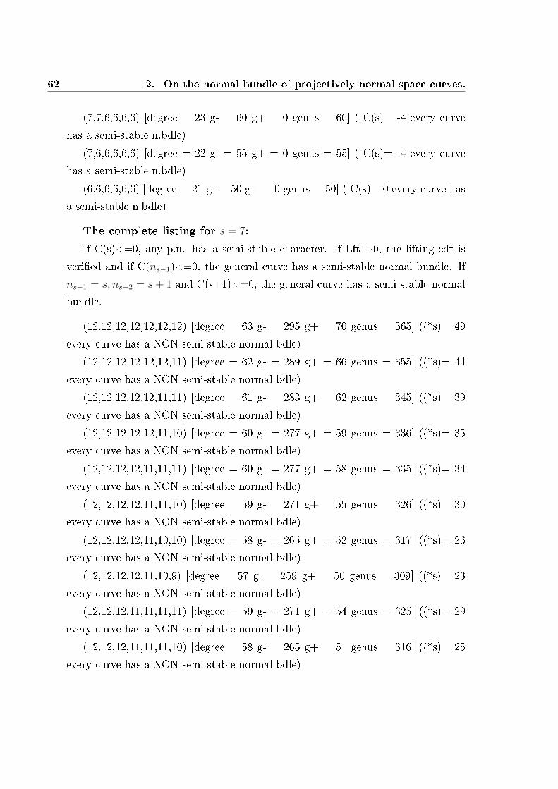
62 2. On the normal bundle of projectively normal space curves.
(7,7,6,6,6,6) [degree = 23 g- = 60 g+ = 0 genus = 60] ( C(s)= -4 every curve
has a semi-stable n.bdle)
(7,6,6,6,6,6) [degree = 22 g- = 55 g+ = 0 genus = 55] ( C(s)= -4 every curve
has a semi-stable n.bdle)
(6,6,6,6,6,6) [degree = 21 g- = 50 g+ = 0 genus = 50] ( C(s)= 0 every curve has
a semi-stable n.bdle)
The complete listing for s = 7:
If C(s)<=0, any p.n. has a semi-stable character. If Lft >0, the lifting cdt is
veried and if C(ns−1)<=0, the general curve has a semi-stable normal bundle. If
ns−1 = s, ns−2 = s+ 1 and C(s+1)<=0, the general curve has a semi stable normal
bundle.
(12,12,12,12,12,12,12) [degree = 63 g- = 295 g+ = 70 genus = 365] ((*s)= 49
every curve has a NON semi-stable normal bdle)
(12,12,12,12,12,12,11) [degree = 62 g- = 289 g+ = 66 genus = 355] ((*s)= 44
every curve has a NON semi-stable normal bdle)
(12,12,12,12,12,11,11) [degree = 61 g- = 283 g+ = 62 genus = 345] ((*s)= 39
every curve has a NON semi-stable normal bdle)
(12,12,12,12,12,11,10) [degree = 60 g- = 277 g+ = 59 genus = 336] ((*s)= 35
every curve has a NON semi-stable normal bdle)
(12,12,12,12,11,11,11) [degree = 60 g- = 277 g+ = 58 genus = 335] ((*s)= 34
every curve has a NON semi-stable normal bdle)
(12,12,12,12,11,11,10) [degree = 59 g- = 271 g+ = 55 genus = 326] ((*s)= 30
every curve has a NON semi-stable normal bdle)
(12,12,12,12,11,10,10) [degree = 58 g- = 265 g+ = 52 genus = 317] ((*s)= 26
every curve has a NON semi-stable normal bdle)
(12,12,12,12,11,10,9) [degree = 57 g- = 259 g+ = 50 genus = 309] ((*s)= 23
every curve has a NON semi-stable normal bdle)
(12,12,12,11,11,11,11) [degree = 59 g- = 271 g+ = 54 genus = 325] ((*s)= 29
every curve has a NON semi-stable normal bdle)
(12,12,12,11,11,11,10) [degree = 58 g- = 265 g+ = 51 genus = 316] ((*s)= 25
every curve has a NON semi-stable normal bdle)

2.7 Appendix 63
(12,12,12,11,11,10,10) [degree = 57 g- = 259 g+ = 48 genus = 307] ((*s)= 21
every curve has a NON semi-stable normal bdle)
(12,12,12,11,11,10,9) [degree = 56 g- = 253 g+ = 46 genus = 299] ((*s)= 18
every curve has a NON semi-stable normal bdle)
(12,12,12,11,10,10,10) [degree = 56 g- = 253 g+ = 45 genus = 298] ((*s)= 17
every curve has a NON semi-stable normal bdle)
(12,12,12,11,10,10,9) [degree = 55 g- = 247 g+ = 43 genus = 290] ((*s)= 14
every curve has a NON semi-stable normal bdle)
(12,12,12,11,10,9,9) [degree = 54 g- = 241 g+ = 41 genus = 282] ((*s)= 11 every
curve has a NON semi-stable normal bdle)
(12,12,12,11,10,9,8) [degree = 53 g- = 235 g+ = 40 genus = 275] ((*s)= 9 every
curve has a NON semi-stable normal bdle)
(12,12,11,11,11,11,11) [degree = 58 g- = 265 g+ = 50 genus = 315] ((*s)= 24
every curve has a NON semi-stable normal bdle)
(12,12,11,11,11,11,10) [degree = 57 g- = 259 g+ = 47 genus = 306] ((*s)= 20
every curve has a NON semi-stable normal bdle)
(12,12,11,11,11,10,10) [degree = 56 g- = 253 g+ = 44 genus = 297] ((*s)= 16
every curve has a NON semi-stable normal bdle)
(12,12,11,11,11,10,9) [degree = 55 g- = 247 g+ = 42 genus = 289] ((*s)= 13
every curve has a NON semi-stable normal bdle)
(12,12,11,11,10,10,10) [degree = 55 g- = 247 g+ = 41 genus = 288] ((*s)= 12
every curve has a NON semi-stable normal bdle)
(12,12,11,11,10,10,9) [degree = 54 g- = 241 g+ = 39 genus = 280] ((*s)= 9 every
curve has a NON semi-stable normal bdle)
(12,12,11,11,10,9,9) [degree = 53 g- = 235 g+ = 37 genus = 272] ((*s)= 6 every
curve has a NON semi-stable normal bdle)
(12,12,11,11,10,9,8) [degree = 52 g- = 229 g+ = 36 genus = 265] ((*s)= 4 every
curve has a NON semi-stable normal bdle)
(12,12,11,10,10,10,10) [degree = 54 g- = 241 g+ = 38 genus = 279] ((*s)= 8
every curve has a NON semi-stable normal bdle)
(12,12,11,10,10,10,9) [degree = 53 g- = 235 g+ = 36 genus = 271] ((*s)= 5 every
curve has a NON semi-stable normal bdle)

64 2. On the normal bundle of projectively normal space curves.
(12,12,11,10,10,9,9) [degree = 52 g- = 229 g+ = 34 genus = 263] ((*s)= 2 every
curve has a NON semi-stable normal bdle)
(12,12,11,10,10,9,8) [degree = 51 g- = 223 g+ = 33 genus = 256] (C(s) =24 is >
0, but C(ns−1)= -18 the general curve has a semi-stable n.bdle)
(12,12,11,10,9,9,9) [degree = 51 g- = 223 g+ = 32 genus = 255] (C(s) =27 is >
0, but C(ns−1)= -39 the general curve has a semi-stable n.bdle)
(12,12,11,10,9,9,8) [degree = 50 g- = 217 g+ = 31 genus = 248] (C(s) =19 is >
0, but C(ns−1)= -23 the general curve has a semi-stable n.bdle)
(12,12,11,10,9,8,8) [degree = 49 g- = 211 g+ = 30 genus = 241] (C(s) =15 is >
0, but C(ns−1)= -27 the general curve has a semi-stable n.bdle)
(12,12,11,10,9,8,7) [degree = 48 g- = 205 g+ = 30 genus = 235] ( C(s)= 0 every
curve has a semi-stable n.bdle)
(12,11,11,11,11,11,11) [degree = 57 g- = 259 g+ = 46 genus = 305] ((*s)= 19
every curve has a NON semi-stable normal bdle)
(12,11,11,11,11,11,10) [degree = 56 g- = 253 g+ = 43 genus = 296] ((*s)= 15
every curve has a NON semi-stable normal bdle)
(12,11,11,11,11,10,10) [degree = 55 g- = 247 g+ = 40 genus = 287] ((*s)= 11
every curve has a NON semi-stable normal bdle)
(12,11,11,11,11,10,9) [degree = 54 g- = 241 g+ = 38 genus = 279] ((*s)= 8 every
curve has a NON semi-stable normal bdle)
(12,11,11,11,10,10,10) [degree = 54 g- = 241 g+ = 37 genus = 278] ((*s)= 7
every curve has a NON semi-stable normal bdle)
(12,11,11,11,10,10,9) [degree = 53 g- = 235 g+ = 35 genus = 270] ((*s)= 4 every
curve has a NON semi-stable normal bdle)
(12,11,11,11,10,9,9) [degree = 52 g- = 229 g+ = 33 genus = 262] ((*s)= 1 every
curve has a NON semi-stable normal bdle)
(12,11,11,11,10,9,8) [degree = 51 g- = 223 g+ = 32 genus = 255] (C(s) =27 is >
0, but C(ns−1)= -15 the general curve has a semi-stable n.bdle)
(12,11,11,10,10,10,10) [degree = 53 g- = 235 g+ = 34 genus = 269] ((*s)= 3
every curve has a NON semi-stable normal bdle)
(12,11,11,10,10,10,9) [degree = 52 g- = 229 g+ = 32 genus = 261] (C(s) =42 is
> 0, but C(ns−1)= -32 the general curve has a semi-stable n.bdle)
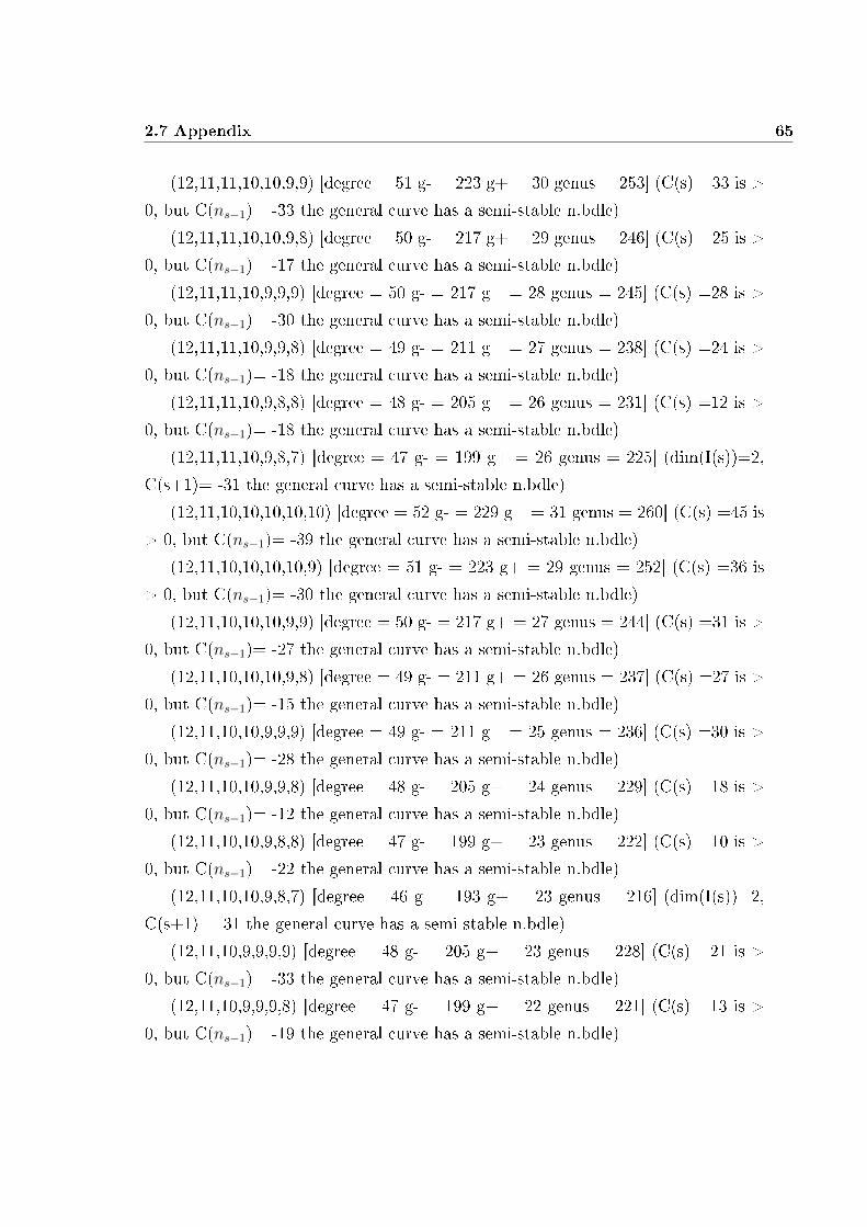
2.7 Appendix 65
(12,11,11,10,10,9,9) [degree = 51 g- = 223 g+ = 30 genus = 253] (C(s) =33 is >
0, but C(ns−1)= -33 the general curve has a semi-stable n.bdle)
(12,11,11,10,10,9,8) [degree = 50 g- = 217 g+ = 29 genus = 246] (C(s) =25 is >
0, but C(ns−1)= -17 the general curve has a semi-stable n.bdle)
(12,11,11,10,9,9,9) [degree = 50 g- = 217 g+ = 28 genus = 245] (C(s) =28 is >
0, but C(ns−1)= -30 the general curve has a semi-stable n.bdle)
(12,11,11,10,9,9,8) [degree = 49 g- = 211 g+ = 27 genus = 238] (C(s) =24 is >
0, but C(ns−1)= -18 the general curve has a semi-stable n.bdle)
(12,11,11,10,9,8,8) [degree = 48 g- = 205 g+ = 26 genus = 231] (C(s) =12 is >
0, but C(ns−1)= -18 the general curve has a semi-stable n.bdle)
(12,11,11,10,9,8,7) [degree = 47 g- = 199 g+ = 26 genus = 225] (dim(I(s))=2,
C(s+1)= -31 the general curve has a semi-stable n.bdle)
(12,11,10,10,10,10,10) [degree = 52 g- = 229 g+ = 31 genus = 260] (C(s) =45 is
> 0, but C(ns−1)= -39 the general curve has a semi-stable n.bdle)
(12,11,10,10,10,10,9) [degree = 51 g- = 223 g+ = 29 genus = 252] (C(s) =36 is
> 0, but C(ns−1)= -30 the general curve has a semi-stable n.bdle)
(12,11,10,10,10,9,9) [degree = 50 g- = 217 g+ = 27 genus = 244] (C(s) =31 is >
0, but C(ns−1)= -27 the general curve has a semi-stable n.bdle)
(12,11,10,10,10,9,8) [degree = 49 g- = 211 g+ = 26 genus = 237] (C(s) =27 is >
0, but C(ns−1)= -15 the general curve has a semi-stable n.bdle)
(12,11,10,10,9,9,9) [degree = 49 g- = 211 g+ = 25 genus = 236] (C(s) =30 is >
0, but C(ns−1)= -28 the general curve has a semi-stable n.bdle)
(12,11,10,10,9,9,8) [degree = 48 g- = 205 g+ = 24 genus = 229] (C(s) =18 is >
0, but C(ns−1)= -12 the general curve has a semi-stable n.bdle)
(12,11,10,10,9,8,8) [degree = 47 g- = 199 g+ = 23 genus = 222] (C(s) =10 is >
0, but C(ns−1)= -22 the general curve has a semi-stable n.bdle)
(12,11,10,10,9,8,7) [degree = 46 g- = 193 g+ = 23 genus = 216] (dim(I(s))=2,
C(s+1)= -31 the general curve has a semi-stable n.bdle)
(12,11,10,9,9,9,9) [degree = 48 g- = 205 g+ = 23 genus = 228] (C(s) =21 is >
0, but C(ns−1)= -33 the general curve has a semi-stable n.bdle)
(12,11,10,9,9,9,8) [degree = 47 g- = 199 g+ = 22 genus = 221] (C(s) =13 is >
0, but C(ns−1)= -19 the general curve has a semi-stable n.bdle)
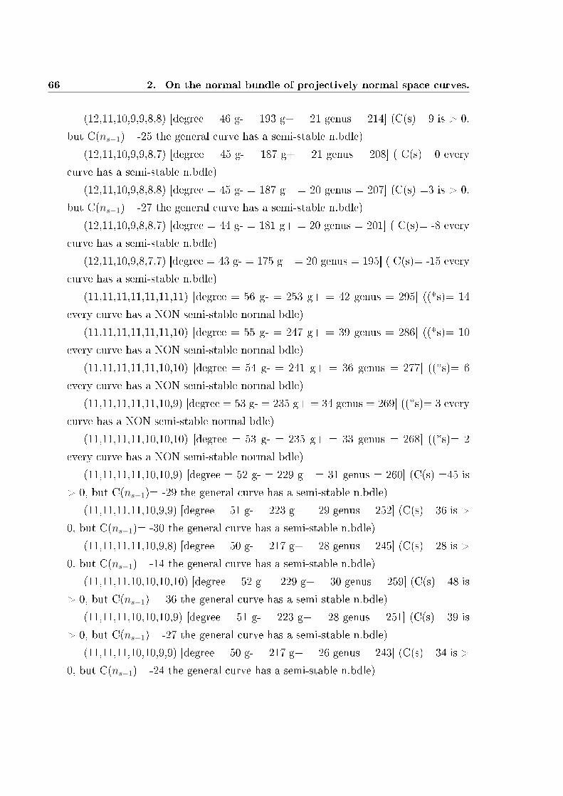
66 2. On the normal bundle of projectively normal space curves.
(12,11,10,9,9,8,8) [degree = 46 g- = 193 g+ = 21 genus = 214] (C(s) =9 is > 0,
but C(ns−1)= -25 the general curve has a semi-stable n.bdle)
(12,11,10,9,9,8,7) [degree = 45 g- = 187 g+ = 21 genus = 208] ( C(s)= 0 every
curve has a semi-stable n.bdle)
(12,11,10,9,8,8,8) [degree = 45 g- = 187 g+ = 20 genus = 207] (C(s) =3 is > 0,
but C(ns−1)= -27 the general curve has a semi-stable n.bdle)
(12,11,10,9,8,8,7) [degree = 44 g- = 181 g+ = 20 genus = 201] ( C(s)= -8 every
curve has a semi-stable n.bdle)
(12,11,10,9,8,7,7) [degree = 43 g- = 175 g+ = 20 genus = 195] ( C(s)= -15 every
curve has a semi-stable n.bdle)
(11,11,11,11,11,11,11) [degree = 56 g- = 253 g+ = 42 genus = 295] ((*s)= 14
every curve has a NON semi-stable normal bdle)
(11,11,11,11,11,11,10) [degree = 55 g- = 247 g+ = 39 genus = 286] ((*s)= 10
every curve has a NON semi-stable normal bdle)
(11,11,11,11,11,10,10) [degree = 54 g- = 241 g+ = 36 genus = 277] ((*s)= 6
every curve has a NON semi-stable normal bdle)
(11,11,11,11,11,10,9) [degree = 53 g- = 235 g+ = 34 genus = 269] ((*s)= 3 every
curve has a NON semi-stable normal bdle)
(11,11,11,11,10,10,10) [degree = 53 g- = 235 g+ = 33 genus = 268] ((*s)= 2
every curve has a NON semi-stable normal bdle)
(11,11,11,11,10,10,9) [degree = 52 g- = 229 g+ = 31 genus = 260] (C(s) =45 is
> 0, but C(ns−1)= -29 the general curve has a semi-stable n.bdle)
(11,11,11,11,10,9,9) [degree = 51 g- = 223 g+ = 29 genus = 252] (C(s) =36 is >
0, but C(ns−1)= -30 the general curve has a semi-stable n.bdle)
(11,11,11,11,10,9,8) [degree = 50 g- = 217 g+ = 28 genus = 245] (C(s) =28 is >
0, but C(ns−1)= -14 the general curve has a semi-stable n.bdle)
(11,11,11,10,10,10,10) [degree = 52 g- = 229 g+ = 30 genus = 259] (C(s) =48 is
> 0, but C(ns−1)= -36 the general curve has a semi-stable n.bdle)
(11,11,11,10,10,10,9) [degree = 51 g- = 223 g+ = 28 genus = 251] (C(s) =39 is
> 0, but C(ns−1)= -27 the general curve has a semi-stable n.bdle)
(11,11,11,10,10,9,9) [degree = 50 g- = 217 g+ = 26 genus = 243] (C(s) =34 is >
0, but C(ns−1)= -24 the general curve has a semi-stable n.bdle)
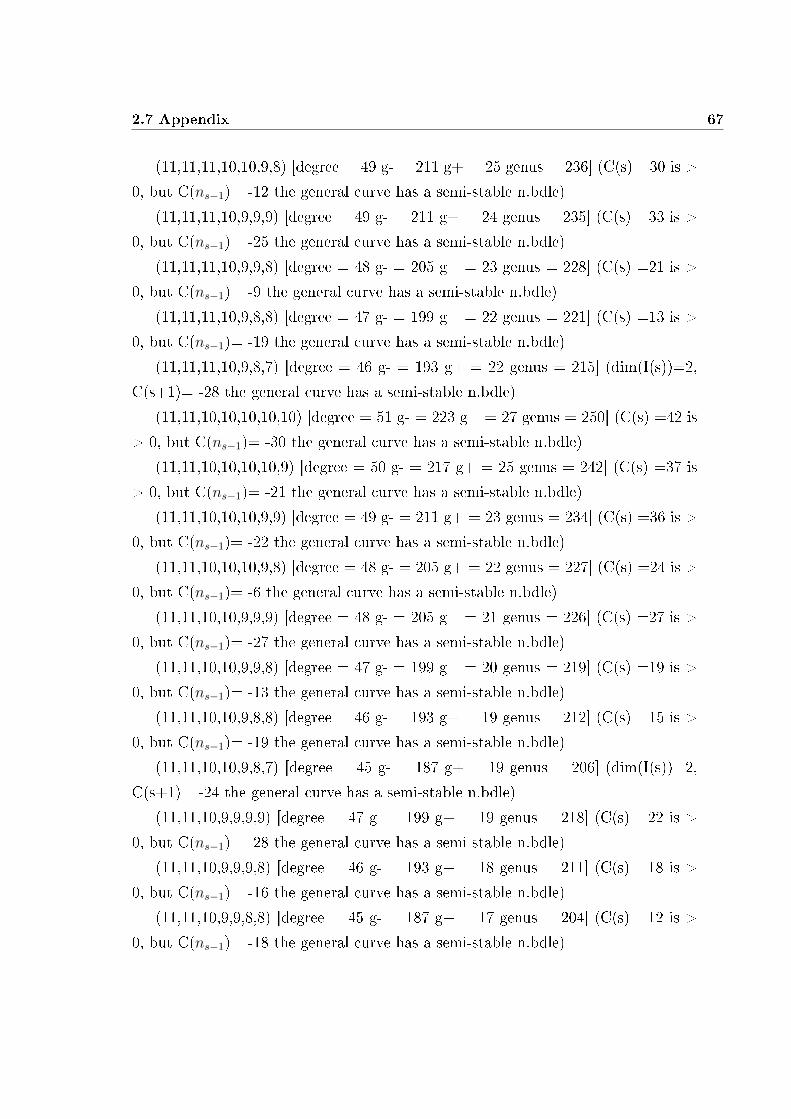
2.7 Appendix 67
(11,11,11,10,10,9,8) [degree = 49 g- = 211 g+ = 25 genus = 236] (C(s) =30 is >
0, but C(ns−1)= -12 the general curve has a semi-stable n.bdle)
(11,11,11,10,9,9,9) [degree = 49 g- = 211 g+ = 24 genus = 235] (C(s) =33 is >
0, but C(ns−1)= -25 the general curve has a semi-stable n.bdle)
(11,11,11,10,9,9,8) [degree = 48 g- = 205 g+ = 23 genus = 228] (C(s) =21 is >
0, but C(ns−1)= -9 the general curve has a semi-stable n.bdle)
(11,11,11,10,9,8,8) [degree = 47 g- = 199 g+ = 22 genus = 221] (C(s) =13 is >
0, but C(ns−1)= -19 the general curve has a semi-stable n.bdle)
(11,11,11,10,9,8,7) [degree = 46 g- = 193 g+ = 22 genus = 215] (dim(I(s))=2,
C(s+1)= -28 the general curve has a semi-stable n.bdle)
(11,11,10,10,10,10,10) [degree = 51 g- = 223 g+ = 27 genus = 250] (C(s) =42 is
> 0, but C(ns−1)= -30 the general curve has a semi-stable n.bdle)
(11,11,10,10,10,10,9) [degree = 50 g- = 217 g+ = 25 genus = 242] (C(s) =37 is
> 0, but C(ns−1)= -21 the general curve has a semi-stable n.bdle)
(11,11,10,10,10,9,9) [degree = 49 g- = 211 g+ = 23 genus = 234] (C(s) =36 is >
0, but C(ns−1)= -22 the general curve has a semi-stable n.bdle)
(11,11,10,10,10,9,8) [degree = 48 g- = 205 g+ = 22 genus = 227] (C(s) =24 is >
0, but C(ns−1)= -6 the general curve has a semi-stable n.bdle)
(11,11,10,10,9,9,9) [degree = 48 g- = 205 g+ = 21 genus = 226] (C(s) =27 is >
0, but C(ns−1)= -27 the general curve has a semi-stable n.bdle)
(11,11,10,10,9,9,8) [degree = 47 g- = 199 g+ = 20 genus = 219] (C(s) =19 is >
0, but C(ns−1)= -13 the general curve has a semi-stable n.bdle)
(11,11,10,10,9,8,8) [degree = 46 g- = 193 g+ = 19 genus = 212] (C(s) =15 is >
0, but C(ns−1)= -19 the general curve has a semi-stable n.bdle)
(11,11,10,10,9,8,7) [degree = 45 g- = 187 g+ = 19 genus = 206] (dim(I(s))=2,
C(s+1)= -24 the general curve has a semi-stable n.bdle)
(11,11,10,9,9,9,9) [degree = 47 g- = 199 g+ = 19 genus = 218] (C(s) =22 is >
0, but C(ns−1)= -28 the general curve has a semi-stable n.bdle)
(11,11,10,9,9,9,8) [degree = 46 g- = 193 g+ = 18 genus = 211] (C(s) =18 is >
0, but C(ns−1)= -16 the general curve has a semi-stable n.bdle)
(11,11,10,9,9,8,8) [degree = 45 g- = 187 g+ = 17 genus = 204] (C(s) =12 is >
0, but C(ns−1)= -18 the general curve has a semi-stable n.bdle)
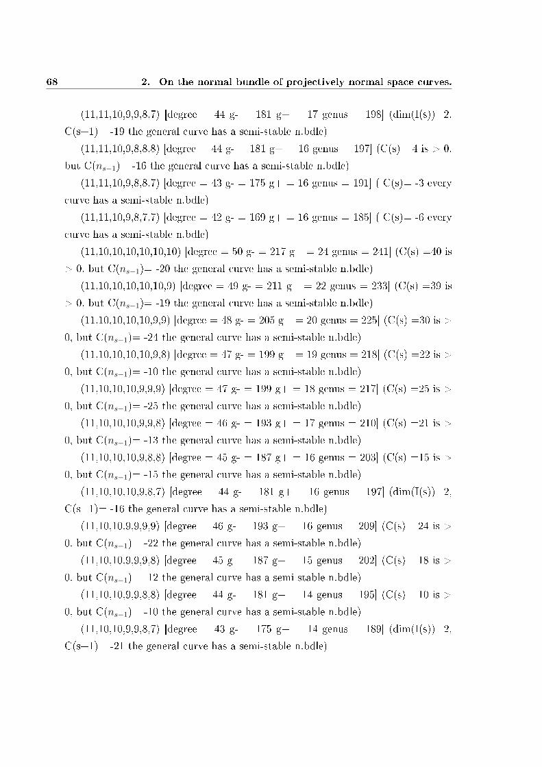
68 2. On the normal bundle of projectively normal space curves.
(11,11,10,9,9,8,7) [degree = 44 g- = 181 g+ = 17 genus = 198] (dim(I(s))=2,
C(s+1)= -19 the general curve has a semi-stable n.bdle)
(11,11,10,9,8,8,8) [degree = 44 g- = 181 g+ = 16 genus = 197] (C(s) =4 is > 0,
but C(ns−1)= -16 the general curve has a semi-stable n.bdle)
(11,11,10,9,8,8,7) [degree = 43 g- = 175 g+ = 16 genus = 191] ( C(s)= -3 every
curve has a semi-stable n.bdle)
(11,11,10,9,8,7,7) [degree = 42 g- = 169 g+ = 16 genus = 185] ( C(s)= -6 every
curve has a semi-stable n.bdle)
(11,10,10,10,10,10,10) [degree = 50 g- = 217 g+ = 24 genus = 241] (C(s) =40 is
> 0, but C(ns−1)= -20 the general curve has a semi-stable n.bdle)
(11,10,10,10,10,10,9) [degree = 49 g- = 211 g+ = 22 genus = 233] (C(s) =39 is
> 0, but C(ns−1)= -19 the general curve has a semi-stable n.bdle)
(11,10,10,10,10,9,9) [degree = 48 g- = 205 g+ = 20 genus = 225] (C(s) =30 is >
0, but C(ns−1)= -24 the general curve has a semi-stable n.bdle)
(11,10,10,10,10,9,8) [degree = 47 g- = 199 g+ = 19 genus = 218] (C(s) =22 is >
0, but C(ns−1)= -10 the general curve has a semi-stable n.bdle)
(11,10,10,10,9,9,9) [degree = 47 g- = 199 g+ = 18 genus = 217] (C(s) =25 is >
0, but C(ns−1)= -25 the general curve has a semi-stable n.bdle)
(11,10,10,10,9,9,8) [degree = 46 g- = 193 g+ = 17 genus = 210] (C(s) =21 is >
0, but C(ns−1)= -13 the general curve has a semi-stable n.bdle)
(11,10,10,10,9,8,8) [degree = 45 g- = 187 g+ = 16 genus = 203] (C(s) =15 is >
0, but C(ns−1)= -15 the general curve has a semi-stable n.bdle)
(11,10,10,10,9,8,7) [degree = 44 g- = 181 g+ = 16 genus = 197] (dim(I(s))=2,
C(s+1)= -16 the general curve has a semi-stable n.bdle)
(11,10,10,9,9,9,9) [degree = 46 g- = 193 g+ = 16 genus = 209] (C(s) =24 is >
0, but C(ns−1)= -22 the general curve has a semi-stable n.bdle)
(11,10,10,9,9,9,8) [degree = 45 g- = 187 g+ = 15 genus = 202] (C(s) =18 is >
0, but C(ns−1)= -12 the general curve has a semi-stable n.bdle)
(11,10,10,9,9,8,8) [degree = 44 g- = 181 g+ = 14 genus = 195] (C(s) =10 is >
0, but C(ns−1)= -10 the general curve has a semi-stable n.bdle)
(11,10,10,9,9,8,7) [degree = 43 g- = 175 g+ = 14 genus = 189] (dim(I(s))=2,
C(s+1)= -21 the general curve has a semi-stable n.bdle)
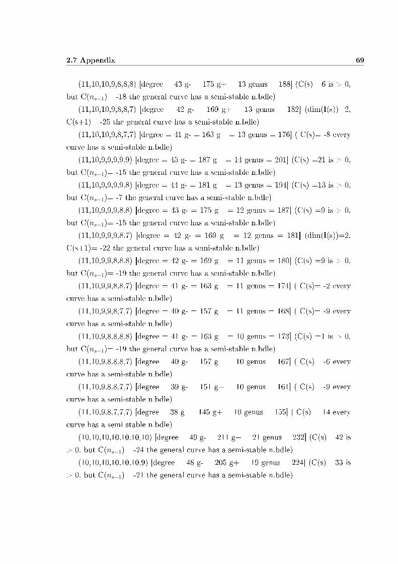
2.7 Appendix 69
(11,10,10,9,8,8,8) [degree = 43 g- = 175 g+ = 13 genus = 188] (C(s) =6 is > 0,
but C(ns−1)= -18 the general curve has a semi-stable n.bdle)
(11,10,10,9,8,8,7) [degree = 42 g- = 169 g+ = 13 genus = 182] (dim(I(s))=2,
C(s+1)= -25 the general curve has a semi-stable n.bdle)
(11,10,10,9,8,7,7) [degree = 41 g- = 163 g+ = 13 genus = 176] ( C(s)= -8 every
curve has a semi-stable n.bdle)
(11,10,9,9,9,9,9) [degree = 45 g- = 187 g+ = 14 genus = 201] (C(s) =21 is > 0,
but C(ns−1)= -15 the general curve has a semi-stable n.bdle)
(11,10,9,9,9,9,8) [degree = 44 g- = 181 g+ = 13 genus = 194] (C(s) =13 is > 0,
but C(ns−1)= -7 the general curve has a semi-stable n.bdle)
(11,10,9,9,9,8,8) [degree = 43 g- = 175 g+ = 12 genus = 187] (C(s) =9 is > 0,
but C(ns−1)= -15 the general curve has a semi-stable n.bdle)
(11,10,9,9,9,8,7) [degree = 42 g- = 169 g+ = 12 genus = 181] (dim(I(s))=2,
C(s+1)= -22 the general curve has a semi-stable n.bdle)
(11,10,9,9,8,8,8) [degree = 42 g- = 169 g+ = 11 genus = 180] (C(s) =9 is > 0,
but C(ns−1)= -19 the general curve has a semi-stable n.bdle)
(11,10,9,9,8,8,7) [degree = 41 g- = 163 g+ = 11 genus = 174] ( C(s)= -2 every
curve has a semi-stable n.bdle)
(11,10,9,9,8,7,7) [degree = 40 g- = 157 g+ = 11 genus = 168] ( C(s)= -9 every
curve has a semi-stable n.bdle)
(11,10,9,8,8,8,8) [degree = 41 g- = 163 g+ = 10 genus = 173] (C(s) =1 is > 0,
but C(ns−1)= -19 the general curve has a semi-stable n.bdle)
(11,10,9,8,8,8,7) [degree = 40 g- = 157 g+ = 10 genus = 167] ( C(s)= -6 every
curve has a semi-stable n.bdle)
(11,10,9,8,8,7,7) [degree = 39 g- = 151 g+ = 10 genus = 161] ( C(s)= -9 every
curve has a semi-stable n.bdle)
(11,10,9,8,7,7,7) [degree = 38 g- = 145 g+ = 10 genus = 155] ( C(s)= -14 every
curve has a semi-stable n.bdle)
(10,10,10,10,10,10,10) [degree = 49 g- = 211 g+ = 21 genus = 232] (C(s) =42 is
> 0, but C(ns−1)= -24 the general curve has a semi-stable n.bdle)
(10,10,10,10,10,10,9) [degree = 48 g- = 205 g+ = 19 genus = 224] (C(s) =33 is
> 0, but C(ns−1)= -21 the general curve has a semi-stable n.bdle)

70 2. On the normal bundle of projectively normal space curves.
(10,10,10,10,10,9,9) [degree = 47 g- = 199 g+ = 17 genus = 216] (C(s) =28 is >
0, but C(ns−1)= -22 the general curve has a semi-stable n.bdle)
(10,10,10,10,10,9,8) [degree = 46 g- = 193 g+ = 16 genus = 209] (C(s) =24 is >
0, but C(ns−1)= -10 the general curve has a semi-stable n.bdle)
(10,10,10,10,9,9,9) [degree = 46 g- = 193 g+ = 15 genus = 208] (C(s) =27 is >
0, but C(ns−1)= -19 the general curve has a semi-stable n.bdle)
(10,10,10,10,9,9,8) [degree = 45 g- = 187 g+ = 14 genus = 201] (C(s) =21 is >
0, but C(ns−1)= -9 the general curve has a semi-stable n.bdle)
(10,10,10,10,9,8,8) [degree = 44 g- = 181 g+ = 13 genus = 194] (C(s) =13 is >
0, but C(ns−1)= -7 the general curve has a semi-stable n.bdle)
(10,10,10,10,9,8,7) [degree = 43 g- = 175 g+ = 13 genus = 188] (dim(I(s))=2,
C(s+1)= -18 the general curve has a semi-stable n.bdle)
(10,10,10,9,9,9,9) [degree = 45 g- = 187 g+ = 13 genus = 200] (C(s) =24 is >
0, but C(ns−1)= -12 the general curve has a semi-stable n.bdle)
(10,10,10,9,9,9,8) [degree = 44 g- = 181 g+ = 12 genus = 193] (C(s) =16 is >
0, but C(ns−1)= -4 the general curve has a semi-stable n.bdle)
(10,10,10,9,9,8,8) [degree = 43 g- = 175 g+ = 11 genus = 186] (C(s) =12 is >
0, but C(ns−1)= -12 the general curve has a semi-stable n.bdle)
(10,10,10,9,9,8,7) [degree = 42 g- = 169 g+ = 11 genus = 180] (dim(I(s))=2,
C(s+1)= -19 the general curve has a semi-stable n.bdle)
(10,10,10,9,8,8,8) [degree = 42 g- = 169 g+ = 10 genus = 179] (C(s) =12 is >
0, but C(ns−1)= -16 the general curve has a semi-stable n.bdle)
(10,10,10,9,8,8,7) [degree = 41 g- = 163 g+ = 10 genus = 173] (dim(I(s))=2,
C(s+1)= -19 the general curve has a semi-stable n.bdle)
(10,10,10,9,8,7,7) [degree = 40 g- = 157 g+ = 10 genus = 167] ( C(s)= -6 every
curve has a semi-stable n.bdle)
(10,10,9,9,9,9,9) [degree = 44 g- = 181 g+ = 11 genus = 192] (C(s) =19 is > 0,
but C(ns−1)= -17 the general curve has a semi-stable n.bdle)
(10,10,9,9,9,9,8) [degree = 43 g- = 175 g+ = 10 genus = 185] (C(s) =15 is > 0,
but C(ns−1)= -9 the general curve has a semi-stable n.bdle)
(10,10,9,9,9,8,8) [degree = 42 g- = 169 g+ = 9 genus = 178] (C(s) =15 is > 0,
but C(ns−1)= -13 the general curve has a semi-stable n.bdle)
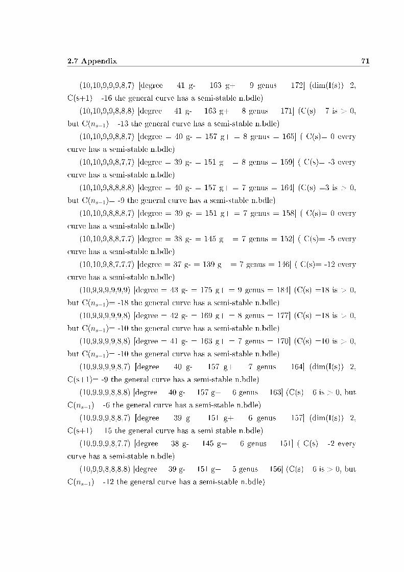
2.7 Appendix 71
(10,10,9,9,9,8,7) [degree = 41 g- = 163 g+ = 9 genus = 172] (dim(I(s))=2,
C(s+1)= -16 the general curve has a semi-stable n.bdle)
(10,10,9,9,8,8,8) [degree = 41 g- = 163 g+ = 8 genus = 171] (C(s) =7 is > 0,
but C(ns−1)= -13 the general curve has a semi-stable n.bdle)
(10,10,9,9,8,8,7) [degree = 40 g- = 157 g+ = 8 genus = 165] ( C(s)= 0 every
curve has a semi-stable n.bdle)
(10,10,9,9,8,7,7) [degree = 39 g- = 151 g+ = 8 genus = 159] ( C(s)= -3 every
curve has a semi-stable n.bdle)
(10,10,9,8,8,8,8) [degree = 40 g- = 157 g+ = 7 genus = 164] (C(s) =3 is > 0,
but C(ns−1)= -9 the general curve has a semi-stable n.bdle)
(10,10,9,8,8,8,7) [degree = 39 g- = 151 g+ = 7 genus = 158] ( C(s)= 0 every
curve has a semi-stable n.bdle)
(10,10,9,8,8,7,7) [degree = 38 g- = 145 g+ = 7 genus = 152] ( C(s)= -5 every
curve has a semi-stable n.bdle)
(10,10,9,8,7,7,7) [degree = 37 g- = 139 g+ = 7 genus = 146] ( C(s)= -12 every
curve has a semi-stable n.bdle)
(10,9,9,9,9,9,9) [degree = 43 g- = 175 g+ = 9 genus = 184] (C(s) =18 is > 0,
but C(ns−1)= -18 the general curve has a semi-stable n.bdle)
(10,9,9,9,9,9,8) [degree = 42 g- = 169 g+ = 8 genus = 177] (C(s) =18 is > 0,
but C(ns−1)= -10 the general curve has a semi-stable n.bdle)
(10,9,9,9,9,8,8) [degree = 41 g- = 163 g+ = 7 genus = 170] (C(s) =10 is > 0,
but C(ns−1)= -10 the general curve has a semi-stable n.bdle)
(10,9,9,9,9,8,7) [degree = 40 g- = 157 g+ = 7 genus = 164] (dim(I(s))=2,
C(s+1)= -9 the general curve has a semi-stable n.bdle)
(10,9,9,9,8,8,8) [degree = 40 g- = 157 g+ = 6 genus = 163] (C(s) =6 is > 0, but
C(ns−1)= -6 the general curve has a semi-stable n.bdle)
(10,9,9,9,8,8,7) [degree = 39 g- = 151 g+ = 6 genus = 157] (dim(I(s))=2,
C(s+1)= -15 the general curve has a semi-stable n.bdle)
(10,9,9,9,8,7,7) [degree = 38 g- = 145 g+ = 6 genus = 151] ( C(s)= -2 every
curve has a semi-stable n.bdle)
(10,9,9,8,8,8,8) [degree = 39 g- = 151 g+ = 5 genus = 156] (C(s) =6 is > 0, but
C(ns−1)= -12 the general curve has a semi-stable n.bdle)
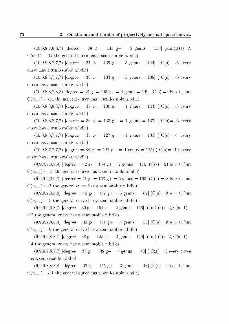
72 2. On the normal bundle of projectively normal space curves.
(10,9,9,8,8,8,7) [degree = 38 g- = 145 g+ = 5 genus = 150] (dim(I(s))=2,
C(s+1)= -17 the general curve has a semi-stable n.bdle)
(10,9,9,8,8,7,7) [degree = 37 g- = 139 g+ = 5 genus = 144] ( C(s)= -6 every
curve has a semi-stable n.bdle)
(10,9,9,8,7,7,7) [degree = 36 g- = 133 g+ = 5 genus = 138] ( C(s)= -9 every
curve has a semi-stable n.bdle)
(10,9,8,8,8,8,8) [degree = 38 g- = 145 g+ = 4 genus = 149] (C(s) =4 is > 0, but
C(ns−1)= -14 the general curve has a semi-stable n.bdle)
(10,9,8,8,8,8,7) [degree = 37 g- = 139 g+ = 4 genus = 143] ( C(s)= -3 every
curve has a semi-stable n.bdle)
(10,9,8,8,8,7,7) [degree = 36 g- = 133 g+ = 4 genus = 137] ( C(s)= -6 every
curve has a semi-stable n.bdle)
(10,9,8,8,7,7,7) [degree = 35 g- = 127 g+ = 4 genus = 131] ( C(s)= -5 every
curve has a semi-stable n.bdle)
(10,9,8,7,7,7,7) [degree = 34 g- = 121 g+ = 4 genus = 125] ( C(s)= -12 every
curve has a semi-stable n.bdle)
(9,9,9,9,9,9,9) [degree = 42 g- = 169 g+ = 7 genus = 176] (C(s) =21 is > 0, but
C(ns−1)= -15 the general curve has a semi-stable n.bdle)
(9,9,9,9,9,9,8) [degree = 41 g- = 163 g+ = 6 genus = 169] (C(s) =13 is > 0, but
C(ns−1)= -7 the general curve has a semi-stable n.bdle)
(9,9,9,9,9,8,8) [degree = 40 g- = 157 g+ = 5 genus = 162] (C(s) =9 is > 0, but
C(ns−1)= -3 the general curve has a semi-stable n.bdle)
(9,9,9,9,9,8,7) [degree = 39 g- = 151 g+ = 5 genus = 156] (dim(I(s))=2, C(s+1)=
-12 the general curve has a semi-stable n.bdle)
(9,9,9,9,8,8,8) [degree = 39 g- = 151 g+ = 4 genus = 155] (C(s) =9 is > 0, but
C(ns−1)= -9 the general curve has a semi-stable n.bdle)
(9,9,9,9,8,8,7) [degree = 38 g- = 145 g+ = 4 genus = 149] (dim(I(s))=2, C(s+1)=
-14 the general curve has a semi-stable n.bdle)
(9,9,9,9,8,7,7) [degree = 37 g- = 139 g+ = 4 genus = 143] ( C(s)= -3 every curve
has a semi-stable n.bdle)
(9,9,9,8,8,8,8) [degree = 38 g- = 145 g+ = 3 genus = 148] (C(s) =7 is > 0, but
C(ns−1)= -11 the general curve has a semi-stable n.bdle)

2.7 Appendix 73
(9,9,9,8,8,8,7) [degree = 37 g- = 139 g+ = 3 genus = 142] ( C(s)= 0 every curve
has a semi-stable n.bdle)
(9,9,9,8,8,7,7) [degree = 36 g- = 133 g+ = 3 genus = 136] ( C(s)= -3 every curve
has a semi-stable n.bdle)
(9,9,9,8,7,7,7) [degree = 35 g- = 127 g+ = 3 genus = 130] ( C(s)= -2 every curve
has a semi-stable n.bdle)
(9,9,8,8,8,8,8) [degree = 37 g- = 139 g+ = 2 genus = 141] (C(s) =3 is > 0, but
C(ns−1)= -9 the general curve has a semi-stable n.bdle)
(9,9,8,8,8,8,7) [degree = 36 g- = 133 g+ = 2 genus = 135] ( C(s)= 0 every curve
has a semi-stable n.bdle)
(9,9,8,8,8,7,7) [degree = 35 g- = 127 g+ = 2 genus = 129] ( We are in the range
of the conjecture BUT CAN'T HANDLE THIS CASE)
(9,9,8,8,7,7,7) [degree = 34 g- = 121 g+ = 2 genus = 123] ( C(s)= -6 every curve
has a semi-stable n.bdle)
(9,9,8,7,7,7,7) [degree = 33 g- = 115 g+ = 2 genus = 117] ( C(s)= -9 every curve
has a semi-stable n.bdle)
(9,8,8,8,8,8,8) [degree = 36 g- = 133 g+ = 1 genus = 134] (C(s) =3 is > 0, but
C(ns−1)= -3 the general curve has a semi-stable n.bdle)
(9,8,8,8,8,8,7) [degree = 35 g- = 127 g+ = 1 genus = 128] (dim(I(s))=2, C(s+1)=
-10 the general curve has a semi-stable n.bdle)
(9,8,8,8,8,7,7) [degree = 34 g- = 121 g+ = 1 genus = 122] ( C(s)= -3 every curve
has a semi-stable n.bdle)
(9,8,8,8,7,7,7) [degree = 33 g- = 115 g+ = 1 genus = 116] ( C(s)= -6 every curve
has a semi-stable n.bdle)
(9,8,8,7,7,7,7) [degree = 32 g- = 109 g+ = 1 genus = 110] ( C(s)= -5 every curve
has a semi-stable n.bdle)
(9,8,7,7,7,7,7) [degree = 31 g- = 103 g+ = 1 genus = 104] ( C(s)= -6 every curve
has a semi-stable n.bdle)
(8,8,8,8,8,8,8) [degree = 35 g- = 127 g+ = 0 genus = 127] (C(s) =7 is > 0, but
C(ns−1)= -7 the general curve has a semi-stable n.bdle)
(8,8,8,8,8,8,7) [degree = 34 g- = 121 g+ = 0 genus = 121] ( C(s)= 0 every curve
has a semi-stable n.bdle)
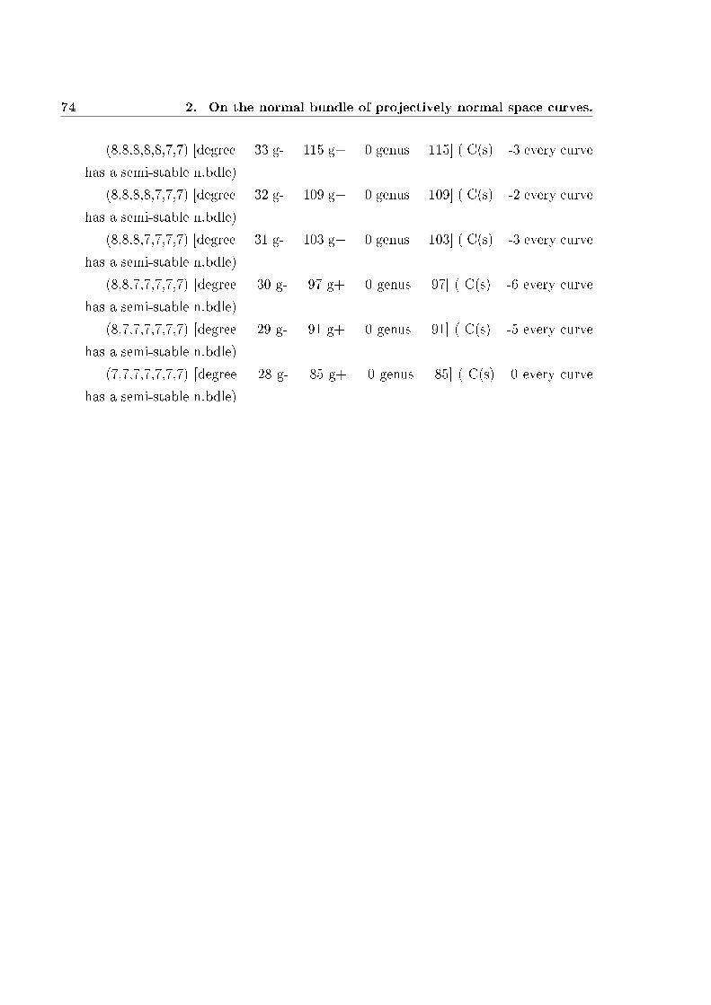
74 2. On the normal bundle of projectively normal space curves.
(8,8,8,8,8,7,7) [degree = 33 g- = 115 g+ = 0 genus = 115] ( C(s)= -3 every curve
has a semi-stable n.bdle)
(8,8,8,8,7,7,7) [degree = 32 g- = 109 g+ = 0 genus = 109] ( C(s)= -2 every curve
has a semi-stable n.bdle)
(8,8,8,7,7,7,7) [degree = 31 g- = 103 g+ = 0 genus = 103] ( C(s)= -3 every curve
has a semi-stable n.bdle)
(8,8,7,7,7,7,7) [degree = 30 g- = 97 g+ = 0 genus = 97] ( C(s)= -6 every curve
has a semi-stable n.bdle)
(8,7,7,7,7,7,7) [degree = 29 g- = 91 g+ = 0 genus = 91] ( C(s)= -5 every curve
has a semi-stable n.bdle)
(7,7,7,7,7,7,7) [degree = 28 g- = 85 g+ = 0 genus = 85] ( C(s)= 0 every curve
has a semi-stable n.bdle)
Chapter 3
Subschemes of P2 with ten fat point
of maximum rank.
3.1 Subschemes of P2 with fat point.
In this section we deal with linear systems of curves of degree d containing zero-
dimensional subschemes of P2. The aim is to understand how determining the
dimension of such systems; we will desume it is not just a mere sum up of conditions.
Let Z be a zero-dimensional subscheme of P2,then we can write Z = b1P1 + ...+
bkPk where Pi's are general points of P2 and where bi ≥ 1 for every i. We simply
denote by bP the point P ∈ P2 with multiplicity b. In other words, bP denotes
the (b-1)-th innitesimal neighborhood of the point P ; let C be a curve, if C has
multiplicity b in P then the curve must contain bP . That is to say, when a curve
C of equation f(x0, x1, x2) = 0 in the local coordinates x0, x1, x2 of P2, contains a
point P of multiplicity b then, any b− 1-th derivative annihilates in P . We deduce
that a point of multiplicity b imposes b(b+1)2
conditions. Let us denote by LZ(d) the
linear system of the curves of degree d containing Z, i.e. all the curves of degree d
in P2 with multiplicity in Pi at least bi. If it is a non-empty system, then we can
compute its dimension as follows:
expdim(LZ(d) :=d(d+ 3)
2−
k∑i=1
bi(bi + 1)
2
75
76 3. Subschemes of P2 with ten fat point of maximum rank.
where d(d+3)2
is the dimension of the linear system of all the curves of degree d in P2,
whereas bi(bi+1)2
is given by the number of conditions imposed by the points Pi's. In
particular, we try to understand which subschemes Z ⊂ P2 are such that, for every
d ∈ N, the linear system LZ(d) has the expected dimension. Clearly, this depends
on the choice of the points in P2 and that's why we always work with general points.
Let us set some useful denitions.
Definition 3.1.1 Let Z be a subscheme of P2, Z has maximum rank if and only if
for all k ∈ Z; h0(IZ(k)) ∗ h1(IZ(k)) = 0, if and only if, for all k ∈ Z the function
H0(OP2(k))→ H0(OZ(k)) is injective or surjective.
Definition 3.1.2 Let Z = b1P1, ..., bkPk a subscheme of P2, of degree z =∑k
i=1bi(bi+1)
2,
then there exist a unique value v such that: h0(OP2(v)) ≥ z, h0(OP2(v − 1)) < z.
This value v is called critical value of Z.
We observe that v = minn ∈ N|(n+2
2
)> z, therefore we expect that every
curve containing Z has degree greater or equal to v. In this setting we can prove
the following equivalence.
Proposition 3.1.3 Let Z be a zero-dimensional subscheme of P2, and let v be its
critical value, then Z has maximum rank if and only if h1(IZ(v)) = 0 and h0(IZ(v−1)) = 0.
Proof:
⇐) Let v be the critical value of Z and let L be a line such that L ∩Z = ∅. We
consider the exact sequence:
0→ O(−1)→ O → OL → 0
twisting by IZ(k) we obtain
0→ IZ(k − 1)→ IZ(k)→ OZ(k)→ 0.
We note that if k ≥ −1 and if h1(IZ(k − 1)) = 0 then h1(IZ(k)) = 0. Since
by hypothesis h1(IZ(v)) = 0, we have h1(IZ(k)) = 0 for all k ≥ v. Moreover if

3.2 Special linear systems of plane curves. 77
h0(IZ(v − 1)) = 0 then h0(IZ(k)) = 0 for all k ≤ v − 1. In conclusion we have
h1(IZ(k)) = 0 for all k ≥ v − 1, h0(IZ(k)) = 0 for all k ≤ v − 1 and so Z has
maximum rank. 2
Remark 3.1.4 Let us consider a subscheme of P2 of maximum rank. Given d ∈ Nsuch that LZ(d) 6= ∅, then h0(IZ(d)) 6= 0 and thus h1(IZ(d)) = 0. This means that:
dim(LZ(d)) = h0(IZ(d)) = h0(OP2(d))− h0(OZ(d)) =d(d+ 3)
2−
k∑i=1
bi(bi + 1)
2=
= expdim(LZ(d)
Finally, if a zero-dimensional subscheme Z of P2 has maximum rank, then, for
every d ∈ N, or LZ(d) = 0 or dim(LZ(d)) = expdim(LZ(d)).
Subschemes of P2 has not maximum rank are very well-known. For instance,
given the following subscheme Z = 2P1 + 2P2 of P2, we note that it has degree z =
22·(2+1)2
= 6 and its critical value is v = 2 since h0(OP2(1)) = 3 and h0(OP2(2)) = 6.
In order Z to have maximum rank, by Proposition 3.1.3 we have that h1(IZ(2)) = 0.
We observe that h1(IZ(2)) = h0(IZ(2)) and since there exists a conic in P2 containing
Z, given by the double line passing through P1 and P2, we have h0(IZ(2)) 6= 0.
Such example guarantees the existence of subschemes in P2 that has not maxi-
mum rank but we can't describe their properties.
3.2 Special linear systems of plane curves.
In this section we deal with special linear systems, L, of plane curves, i.e. those
systems with h1(L) 6= 0 in cohomology. Concerning the dimensional problem of
such systems, there exists a particular conjecture called Harbourne-Hirschowitz's
conjecture.
Let us introduce some denitions:
Definition 3.2.1 Let Z = b1P1+...+bnPn be a subscheme of P2. The linear system
of plane curves of degree d containing Z, LZ(d) is said non-special if h1(LZ(d)) = 0.
Otherwise the linear system is said special.

78 3. Subschemes of P2 with ten fat point of maximum rank.
Going back to the previous section, given a zero-dimensional subscheme Z in
P2, if LZ(d) 6= 0 is a non-special linear system, then h1(LZ(d)) = 0 and thus
dim(LZ(d)) = expdim(LZ(d)). We deduce that if Z has maximum rank, the linear
system LZ(d) is zero or non-special.
In the literature, the rst conjecture about special linear systems goes back to
B. Segre. It states the following:
Conjecture 3.2.2 If a linear system of plane curves with general multiple base
points LZ(d) is special, then one of its general member is non-reduced, namely the
linear system has, according to Bertini's theorem, some multiple xed component.
Such a conjecture deduce the existence of a double curve in the special linear
system of curves in P2. Later on, Hirschowitz and Harbourne determine a new
property of the double curve: it is, in fact, an exceptional curve of the system in his
locus.
Let us dene an exceptional curve.
Let us consider the blow-up π : P2 → P2 of the plane P2 at P1, ..., Pn. Let
E1, ..., En be the exceptional divisors corresponding to the blow-up points P1, ..., Pn
and let H be the pull-back of a general line of P2 via π. The strict transform of the
linear system LZ(d), where Z = b1P1 + ...+ bnPn, is
LZ(d) := |dH − b1E1 − ... − bnEn|. In the system LZ(d), the rules intersection are
the following:
H2 = 1;
Ei · Ej = δij.
Definition 3.2.3 A curve C ⊂ P2 is said exceptional curve if it is a rational curve
and with self-intersection -1.
For instance, every exceptional divisor is an exceptional curve, such as any line
passing through two blow-up points.
Now, let us state Harbourne-Hirschowitz's conjecture:
Conjecture 3.2.4 A linear system of plane curve L, with general multiple base
points is special if and only if there exists an exceptional curve with multiplicity at
least two in the base locus.

3.2 Special linear systems of plane curves. 79
Let us go back to the example in the rst section, the linear system LZ(2) with
Z = 2P1 + 2P2. Since h0(IZ(2)) 6= 0, the sequence
0→ H0(IZ(2))→ H0(OP2)→ H0(OZ(2))→ ...
is not short exact, therefore h1(IZ(2)) 6= 0 and the system is special. Now, let us
consider the line R = H − E1 − E2 passing through P1, P2. We note that R2 = −1
and, since 2R is the only curve in LZ(2), such a line is in the locus of the system
with multiplicity two.
In order to see more examples, let us consider a subscheme Z in P2 of the form
Z = 2P1 + ... + 2P d(d+3)2
and the linear system LZ(2d), with d < 4. It is easy to
prove that the curve of degree d passing through Pi is an exceptional curve and it
is in the locus of LZ(2d) with multiplicity two.
More generally, one has special linear systems in the following situation. Let Lbe a linear system on P2 which is, non-empty and let C be an exceptional curve
on P2 corresponding to a curve Γ on P2, such that L · · ·C = −N < 0. Then C
(respectively Γ ) splits o with multiplicity N as a xed component from all curves
of L (respectively L) and one has:
L = NC + M(respectivelyL = NΓ +M)
where M (resp. M) is the residual linear system. We can see that if N ≥ 2,
then L is special.
Even more generally, consider a linear system L on P2 non-empty , C1, ...Ck
exceptional curves on P2 corresponding to curves Γ1, ..., Γk on P2, such that L ·Ci =
−Ni < 0, i = 1, .., k. Then:
L =k∑i=1
NiCi + M,L =k∑i=1
NiΓi +M
and M · Ci = 0 for i = 1, .., k. As before, L is special as soon as there exists an
i = 1, ..., k such that Ni ≥ 2. Furthermore CiCj = −δij and C :=∑k
i=1Ci is called
(-1)-conguration on P2. Now we give another denition.
80 3. Subschemes of P2 with ten fat point of maximum rank.
Definition 3.2.5 A linear system L on P2 is called (-1)-special if, L =∑k
i=1NiCi+
M where C =∑k
i=1 Ci is a (-1)-conguration, MCi = 0, for all i = 1, .., k,
dim(M) ≥ 0 and there exists an i = 1, ..., k such that Ni > 1.
We want to remember that in the work of Ciliberto, they were classied every
homogeneous linear system which are (-1)-special. Until now, we can nd only these
linear systems as examples of special linear systems. The theorem is the following:
Theorem 3.2.6 (C.Ciliberto) The only homogeneous linear systems LZ(d), where
Z = mP1 + ...+mPh is a subscheme of P2, which are (-1)-special are:
LZ(d) with Z = mP1 + mP2 and with m ≤ d ≤ 2m− 2 LZ(d) with Z = mP1 +
mP2+mP3 and with 32m ≤ d ≤ 2m−2 LZ(d) with Z = mP1+mP2+mP3+mP4+mP5
and with 2m ≤ d ≤ 5m−22LZ(d) with Z = mP1 +mP2 +mP3 +mP4 +mP5 +mP6 and
with 125m ≤ d ≤ 5m−2
2LZ(d) with Z = mP1 +mP2 +mP3 +mP4 +mP5 +mP6 +mP7
and with 218m ≤ d ≤ 8m−2
3LZ(d) with Z = mP1 +mP2 +mP3 +mP4 +mP5 +mP6 +
mP7 +mP8 and with 4817m ≤ d ≤ 17m−2
6
As a remarkable consequence we have that the Harbourne-Hirschowitz conjecture
for homogeneous system take the form:
Conjecture 3.2.7 Every homogeneous system of the form LZ(d), where Z =
mP1 + ...+mPh is a subscheme of P2, with h ≥ 10, is non-special.
Moreover we can prove that if the Harbourne-Hirschowitz conjecture hold, then
the system L on P2 is special if and only if it is (-1)-special, and so the linear systems
of theorem 3.2.6 could be the only special systems.
Many other people studied the Harbourne-Hirschowitz conjecture. Now we want
to enunciate the most important result of this study.
Hirschowitz worked on this conjecture and formulated the following theorem:
Theorem 3.2.8 (Hirschowitz) The Harbourne-Hirschowitz conjecture holds in the
homogeneous case LZ(d) with Z = mP1 + ...+mPh subscheme of P2, with m ≤ 3.
To prove this theorem he uses a degeneration technique called the Horace's
method, which we will deal with in the next section. The application of Horace's

3.2 Special linear systems of plane curves. 81
method usually requires a deep geometric understanding of the problem and a special
capability of guessing the right specializations to be performed.
Afterward Ciliberto and Miranda proved the following theorem:
Theorem 3.2.9 The Harbourne-Hirschowitz conjecture holds in the quasi-homogeneous
cases, LZ, where Z = nP1 +mP2 + ...+mPh is a subscheme of P2 with m ≤ 3 and
in the homogeneous case, LZ, where Z = +mP1 + ... + mPh is a subscheme of P2
with m ≤ 12.
Despite of Hirschowitz technique, the idea of Ciriberto and Miranda which I will
explain in some detail, consists in using a degeneration technique worked out by
Z. Ran manly for studying enumerative problems of families of plane nodal curves.
It consists in degenerating the plane to a reducible surface and in following the
linear system in the degeneration. The restriction of the limit linear system to the
component of the reducible limit surface are easier than the system one starts with,
so that one can hope to successfully use induction.
Another important result is due to S. Yang:
Theorem 3.2.10 The Harbourne-Hirschowitz conjecture holds for all linear sys-
tems of plane curves with at most ten points having multiplicity up to seven.
S. Yang approach to this problem has a simple geometric description. Suppose
we are given a linear system LZ of a plane curve with multiple base point. Choose
a triangle of three lines in P2 that meet in three distinct points. We specialize the
base points by moving them onto these points and sliding the multiple points along
the three lines to collide them. Each collision creates a larger singularity in the base
locus of the limiting linear system, and the class of singularities that arise can be
completely described via a combinatorial game involving checkers on a triangular
board.
The second technique, used by S. Yang is a modication of a well-known degenera-
tion, rst exploited by Ciliberto and Miranda.
I want to start just from this result. As a matter of fact we will prove with this
thesis that such result is also valid, even if we have 10 points of multiplicity at most
eight. Actually, we will be able to do better, as we will prove that every subscheme
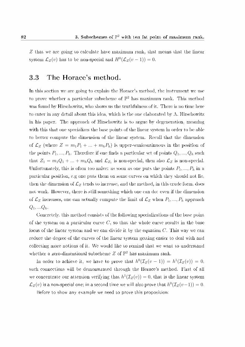
82 3. Subschemes of P2 with ten fat point of maximum rank.
Z that we are going to calculate have maximum rank, that means that the linear
system LZ(v) has to be non-special and H0(LZ(v − 1)) = 0.
3.3 The Horace's method.
In this section we are going to explain the Horace's method, the instrument we use
to prove whether a particular subscheme of P2 has maximum rank. This method
was found by Hirschowitz, who shows us the truthfulness of it. There is no time here
to enter in any detail about this idea, which is the one elaborated by A. Hirschowitz
in his paper. The approach of Hirschowitz is to argue by degeneration, meaning
with this that one specializes the base points of the linear system in order to be able
to better compute the dimension of the linear system. Recall that the dimension
of LZ (where Z = m1P1 + ... + mhPh) is upper-semicontinuous in the position of
the points P1, ..., Ph. Therefore if one nds a particular set of points Q1, ..., Qh such
that Z1 = m1Q1 + ... + mhQh and LZ1 is non-special, then also LZ is non-special.
Unfortunately, this is often too naive: as soon as one puts the points P1, ..., Ph in a
particular position, e.g one puts them on some curves on which they should not lie,
then the dimension of LZ tends to increase, and the method, in this crude form, does
not work. However, there is still something which one can do: even if the dimension
of LZ increases, one can actually compute the limit of LZ when P1, ..., Ph approach
Q1, ...Qh.
Concretely, this method consists of the following specializations of the base point
of the system on a particular curve C, so that the whole curve results in the base
locus of the linear system and we can divide it by the equation C. This way we can
reduce the degree of the curves of the linear system getting easier to deal with and
collecting more notions of it. We would like to remind that we want to understand
whether a zero-dimensional subscheme Z of P2 has maximum rank.
In order to achieve it, we have to prove that h0(IZ(v − 1)) = h1(IZ(v)) = 0,
such connections will be demonstrated through the Horace's method. First of all
we concentrate our attention verifying that h1(IZ(v)) = 0, that is the linear system
LZ(v) is a non-special one; in a second time we will also prove that h0(IZ(v−1)) = 0.
Before to show any example we need to prove this proposition:

3.3 The Horace's method. 83
Proposition 3.3.1 Let C,D be two subscheme of P2 such that C ⊂ D. If LD(d)
is non-special, then LC(d) is non-special too, where with LC(d) we denote the linear
system IZ(d).
Dimostrazione:
As C ⊂ D, the exact sequence is true:
0→ ID(d)→ IC(d)→ IC,D → 0
In cohomology we obtain:
...→ H1(ID(d))→ H1(IC(d))→ 0
Since the support of IC,D is zero-dimensional, then h1(IC,D) = 0 and it's clear that
if ID(d) = 0 then IC(d) = 0 too. 2
We give some notations. We denote by (n) a fat point of multiplicity n and we
represent it as follows
n
while we will represent a simple point as a little black disk. We bring a simple
example about the use of the Horace's method.
Example 3.3.2 Let Z = 2P1 + 2P2 + ...+ 2P10 be a subscheme of P2, Z has degree
equal to 10·3 = 30 and critical value 7 because h0(OP2(6)) = 28 and h0(OP2(7)) = 36.
We must prove that h1(IZ(7)) = 0 thus we need that h0(IZ(7)) = h0(OP2(7)) −h0(OZ(7)) = 36−30 = 6 and so it is sucient to show that h0(IZ(7)) = 6. Now, let
us take a new subscheme Z1 = Z + P11 + ...+ P16, composed by Z and by other six
points in general position. This subscheme has degree 36 and so the linear system
IZ1(7) is non-special if and only if h0(IZ1) = 0. Specializing the points of Z1 we
show that there doesn't exist any curve of degree 7 containing Z1, therefore IZ1(7) is
non-special and by proposition 3.3.1, IZ(7) is non-special too.
With notations as above, we represent the subscheme Z1 by 10 double points, (2)
and by 6 simple points. We start specializing seven double points and a normal point

84 3. Subschemes of P2 with ten fat point of maximum rank.
in a conic curve C, outside we have three double points and ve points. On C we
have 7 ∗ 2 + 1 = 15 = 2 ∗ 7 + 1 conditions. So we can divide by the equation of the
conic and reduce to the following situation for the curves of degree ve (i.e.v = 5).
v = 7 2 5
22
v = 5 25
We divide by eq. of conic
3
22222
3
We have on C seven simple points, outside of C there are three (2) and ve simple
points. Now we specialize other two (2) on C.
v = 5 25
22
On conic we have 2 ∗ 2 + 7 = 11 = 5 ∗ 2 + 1 conditions and so we can divide
by the equations of conic and we obtain the following situation for curves of degree
three.
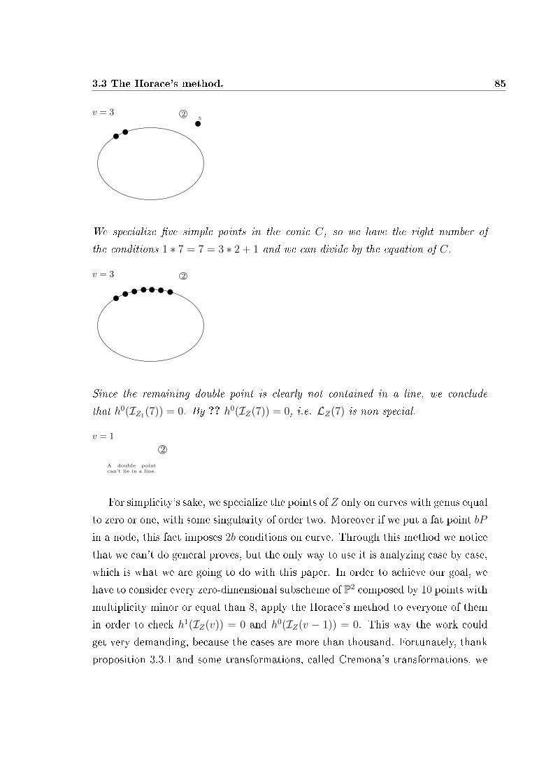
3.3 The Horace's method. 85
v = 3 25
We specialize ve simple points in the conic C, so we have the right number of
the conditions 1 ∗ 7 = 7 = 3 ∗ 2 + 1 and we can divide by the equation of C.
v = 3 2
Since the remaining double point is clearly not contained in a line, we conclude
that h0(IZ1(7)) = 0. By ?? h0(IZ(7)) = 0, i.e. LZ(7) is non-special.
2
v = 1
A double pointcan’t lie in a line.
For simplicity's sake, we specialize the points of Z only on curves with genus equal
to zero or one, with some singularity of order two. Moreover if we put a fat point bP
in a node, this fact imposes 2b conditions on curve. Through this method we notice
that we can't do general proves, but the only way to use it is analyzing case by case,
which is what we are going to do with this paper. In order to achieve our goal, we
have to consider every zero-dimensional subscheme of P2 composed by 10 points with
multiplicity minor or equal than 8, apply the Horace's method to everyone of them
in order to check h1(IZ(v)) = 0 and h0(IZ(v − 1)) = 0. This way the work could
get very demanding, because the cases are more than thousand. Fortunately, thank
proposition 3.3.1 and some transformations, called Cremona's transformations, we
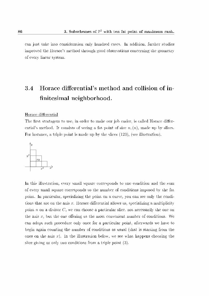
86 3. Subschemes of P2 with ten fat point of maximum rank.
can just take into consideration only hundred cases. In addition, further studies
improved the Horace's method through good observations concerning the geometry
of every linear system.
3.4 Horace dierential's method and collision of in-
nitesimal neighborhood.
Horace dierential
The rst stratagem to use, in order to make our job easier, is called Horace dier-
ential's method. It consists of seeing a fat point of size n, (n), made up by slices.
For instance, a triple point is made up by the slices (123), (see illustration).
y
xx2
xy
y2
In this illustration, every small square corresponds to one condition and the sum
of every small square corresponds to the number of conditions imposed by the fat
point. In particular, specializing the point on a curve, you can see only the condi-
tions that are on the axis x. Horace dierential allows us, specializing a multiplicity
point n on a divisor C, we can choose a particular slice, not necessarily the one on
the axis x, but the one oering us the most convenient number of conditions. We
can adopt such procedure only once for a particular point, afterwards we have to
begin again counting the number of conditions as usual (that is starting from the
ones on the axis x). In the illustration below, we see what happens choosing the
slice giving us only two conditions from a triple point (3).

3.4 Horace dierential's method and collision of innitesimal neighborhood. 87
y
xx2
xy
y2
y
xx
y
To represent this situation on a curve, we use a more convenient notation to our
aim as in gure.
2
[1,3]
where the notation [1, 3] represents the remaining slices.
Dividing by the equation of C, it occurs.
3
[1]
We rest with three conditions on C and, dividing by equation of the curve, we
remain with only one condition on C.
In general we represent the slice m of a fat point (n) as in the following picture:
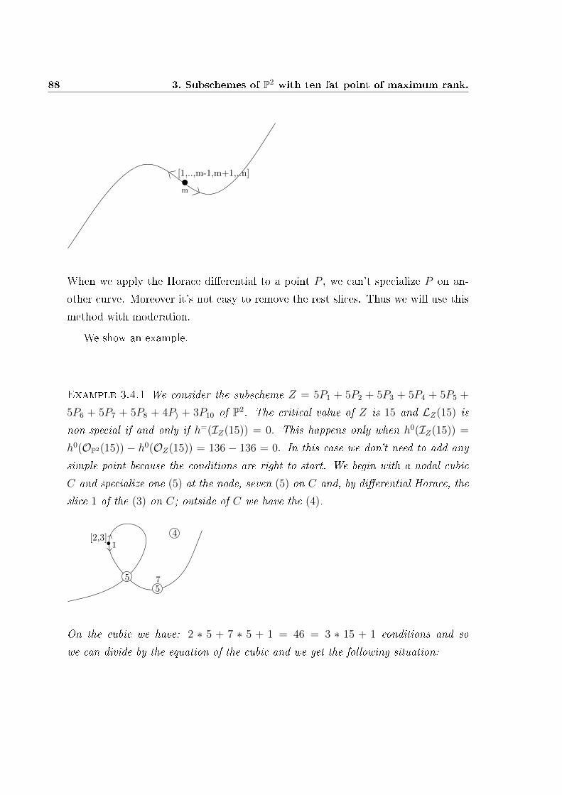
88 3. Subschemes of P2 with ten fat point of maximum rank.
m
[1,..,m-1,m+1,..n]
When we apply the Horace dierential to a point P , we can't specialize P on an-
other curve. Moreover it's not easy to remove the rest slices. Thus we will use this
method with moderation.
We show an example.
Example 3.4.1 We consider the subscheme Z = 5P1 + 5P2 + 5P3 + 5P4 + 5P5 +
5P6 + 5P7 + 5P8 + 4P) + 3P10 of P2. The critical value of Z is 15 and LZ(15) is
non-special if and only if h=(IZ(15)) = 0. This happens only when h0(IZ(15)) =
h0(OP2(15)) − h0(OZ(15)) = 136 − 136 = 0. In this case we don't need to add any
simple point because the conditions are right to start. We begin with a nodal cubic
C and specialize one (5) at the node, seven (5) on C and, by dierential Horace, the
slice 1 of the (3) on C; outside of C we have the (4).
55
4
7
[2,3]1
On the cubic we have: 2 ∗ 5 + 7 ∗ 5 + 1 = 46 = 3 ∗ 15 + 1 conditions and so
we can divide by the equation of the cubic and we get the following situation:
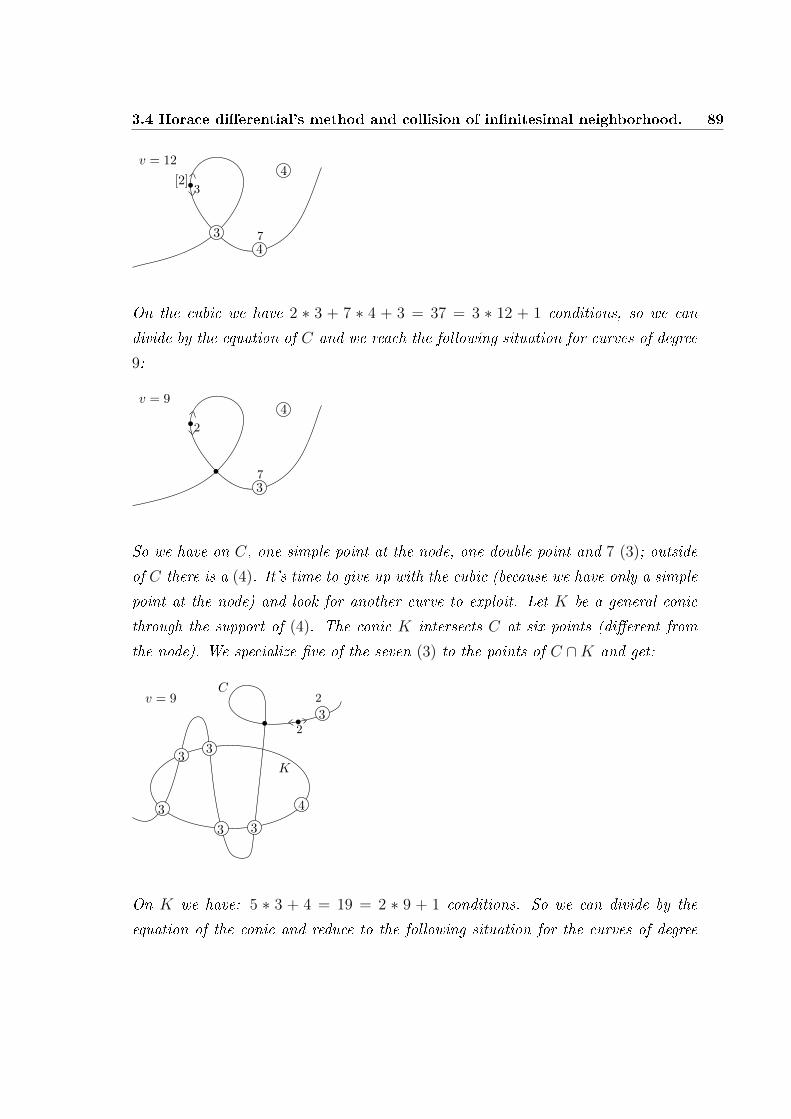
3.4 Horace dierential's method and collision of innitesimal neighborhood. 89
34
4
7
[2]3
v = 12
On the cubic we have 2 ∗ 3 + 7 ∗ 4 + 3 = 37 = 3 ∗ 12 + 1 conditions, so we can
divide by the equation of C and we reach the following situation for curves of degree
9:
3
4
7
2
v = 9
So we have on C, one simple point at the node, one double point and 7 (3); outside
of C there is a (4). It's time to give up with the cubic (because we have only a simple
point at the node) and look for another curve to exploit. Let K be a general conic
through the support of (4). The conic K intersects C at six points (dierent from
the node). We specialize ve of the seven (3) to the points of C ∩K and get:
v = 9
33
3
3 3
3
4
2
C
K
2
On K we have: 5 ∗ 3 + 4 = 19 = 2 ∗ 9 + 1 conditions. So we can divide by the
equation of the conic and reduce to the following situation for the curves of degree
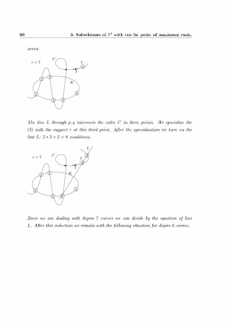
90 3. Subschemes of P2 with ten fat point of maximum rank.
seven:
v = 7
2
3
3
2
C
K
2
2
2
2 2
The line L through p, q intersects the cubic C in three points. We specialize the
(3) with the support r at this third point. After the specialization we have on the
line L: 2 ∗ 3 + 2 = 8 conditions.
v = 7
2
3
3
2
C
K
2
2
2
2 2
3
L
Since we are dealing with degree 7 curves we can divide by the equation of line
L. After this reduction we remain with the following situation for degree 6 curves.
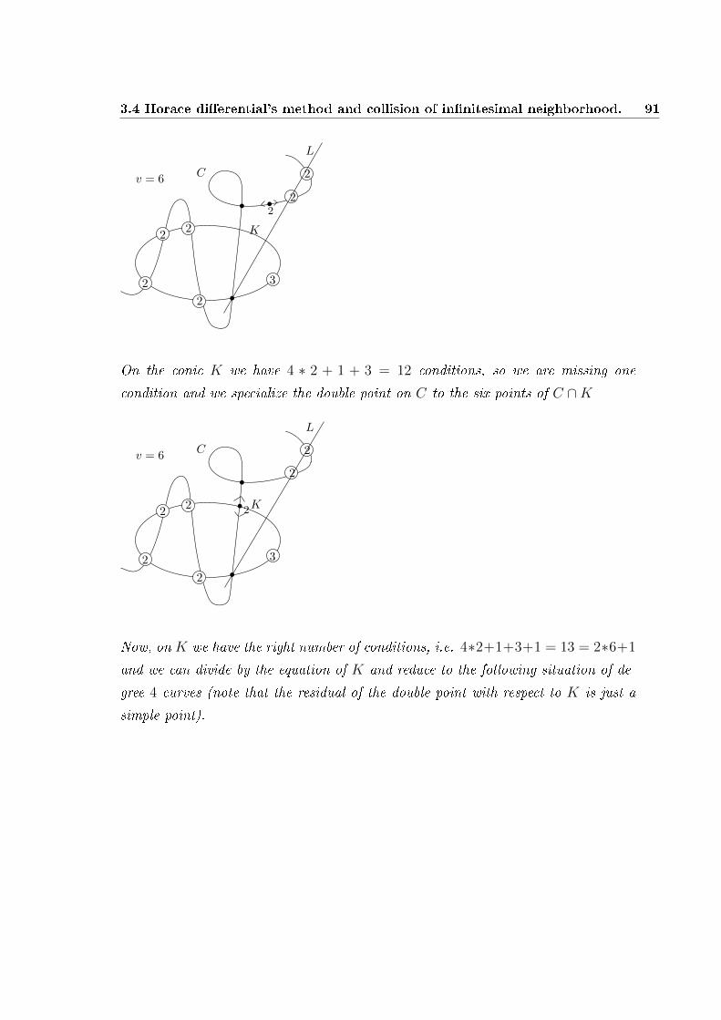
3.4 Horace dierential's method and collision of innitesimal neighborhood. 91
v = 6
2
2
3
2
C
K2
2
2
2
L
On the conic K we have 4 ∗ 2 + 1 + 3 = 12 conditions, so we are missing one
condition and we specialize the double point on C to the six points of C ∩K
v = 6
2
2
3
2
C
K2
2
2
2
L
Now, on K we have the right number of conditions, i.e. 4∗2+1+3+1 = 13 = 2∗6+1
and we can divide by the equation of K and reduce to the following situation of de-
gree 4 curves (note that the residual of the double point with respect to K is just a
simple point).
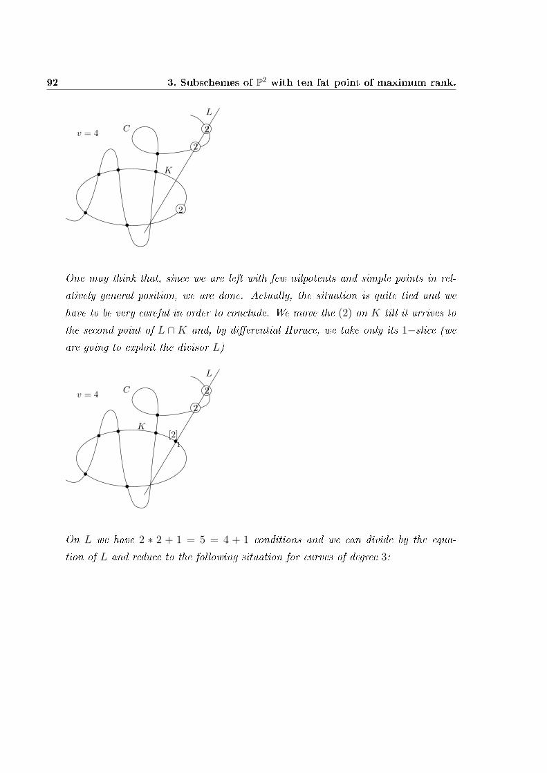
92 3. Subschemes of P2 with ten fat point of maximum rank.
v = 4
2
2
C
K
2
L
One may think that, since we are left with few nilpotents and simple points in rel-
atively general position, we are done. Actually, the situation is quite tied and we
have to be very careful in order to conclude. We move the (2) on K till it arrives to
the second point of L ∩K and, by dierential Horace, we take only its 1−slice (we
are going to exploit the divisor L)
v = 4
2
[2]
C
K
2
L
1
On L we have 2 ∗ 2 + 1 = 5 = 4 + 1 conditions and we can divide by the equa-
tion of L and reduce to the following situation for curves of degree 3:
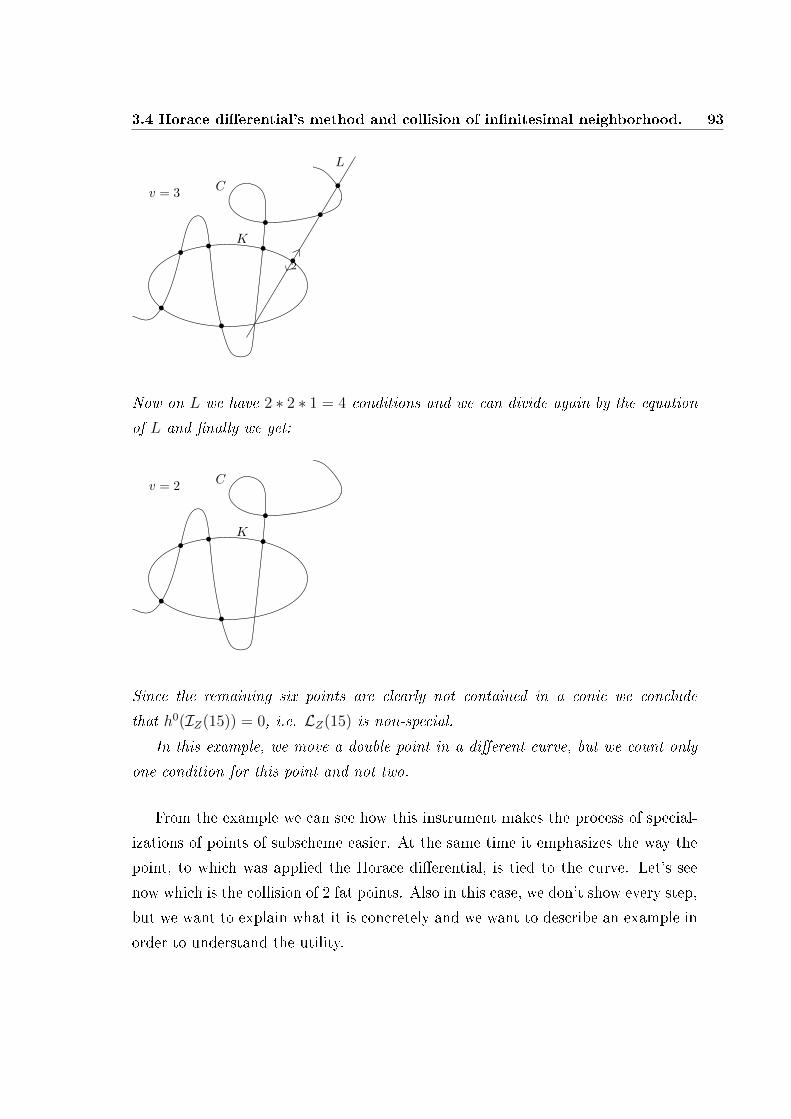
3.4 Horace dierential's method and collision of innitesimal neighborhood. 93
v = 3
2
C
K
L
Now on L we have 2 ∗ 2 ∗ 1 = 4 conditions and we can divide again by the equation
of L and nally we get:
v = 2C
K
Since the remaining six points are clearly not contained in a conic we conclude
that h0(IZ(15)) = 0, i.e. LZ(15) is non-special.
In this example, we move a double point in a dierent curve, but we count only
one condition for this point and not two.
From the example we can see how this instrument makes the process of special-
izations of points of subscheme easier. At the same time it emphasizes the way the
point, to which was applied the Horace dierential, is tied to the curve. Let's see
now which is the collision of 2 fat points. Also in this case, we don't show every step,
but we want to explain what it is concretely and we want to describe an example in
order to understand the utility.
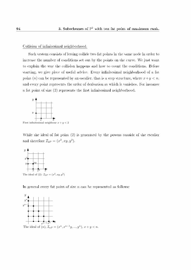
94 3. Subschemes of P2 with ten fat point of maximum rank.
Collision of innitesimal neighborhood.
Such system consists of letting collide two fat points in the same node in order to
increase the number of conditions set out by the points on the curve. We just want
to explain the way the collision happens and how to count the conditions. Before
starting, we give piece of useful advice. Every innitesimal neighborhood of a fat
point (n) can be represented by an escalier, that is a step structure, where x+y < n,
and every point represents the order of derivation at which it vanishes. For instance
a fat point of size (2) represents the rst innitesimal neighborhood.
x
y
First infinitesimal neighbour x + y < 2
y
x
While the ideal of fat point (2) is generated by the powers outside of the escalier
and therefore I2P = (x2, xy, y2).
x
y
y
x x2
y2
xy
The ideal of (2): I2P = (x2, xy, y2)
In general every fat point of size n can be represented as follows:
xn
yn
x
y
The ideal of (n), InP = (xn, xn−1y, ..., yn), x+ y < n.
yn−1
xn−1

3.4 Horace dierential's method and collision of innitesimal neighborhood. 95
In order to proceed with the collision, we have to privilege an axis. We choose the
one of the y, that we indicate as the collision axis. In view of that, we notice that an
escalier e determines a function e : N→ N : x→ e(x) so that e = (x, y)|y < e(x)
x
e(x)
Given two escaliers, we can dene the operation of the sum in this way. Let e1, e2 be
two escalier, then the sum e1 + e2 is an escalier too, such that ˆe1 + e2 = e1 + e2. In
practice, we are placing an escalier upon another one, letting slide the several small
squares along the axis y.(see illustration)
Point of multiplicity 3, (3)
x
y
Double point (2)
x
y
y
xCollision in the direction y of the fat point (2) e (3)
This is the sum along the vertical axis y, that we have considered as collision
axis.
Now we have to try to join what we have said so far with the Horace's method.
Therefore, we presume to have a double point on a node of a nodal cubic and a
point of multiplicity (3), on a branch of the same cubic, (see illustration):

96 3. Subschemes of P2 with ten fat point of maximum rank.
2
3
Doing the collision according the direction →, we get:
y
x
3
5
Whose trace on the curve has 5 + 3 = 8 degrees, because, being on a node, one
has to count as the conditions on the x axis, the ones on the y axis. For such point
we have to use the numbering [32211].
Considering this sequence of numbers as 32, 21, 1, these indicate the number of
conditions which there are in the rst, second and third column of the illustration
shown above( i.e. after the collision of (3) with (2)). As matter of fact, in the rst
column there are 3 + 2 = 5, in the second 2 + 1 = 3 and in the third one only a
small square is left. Before the collision, the number of the conditions was given by
2 · 2 + 3 = 7. Therefore we increase by one the number of the conditions. Dividing
by equation of cubic, the rest of collision results:
x
y
Double point along the direction ↑
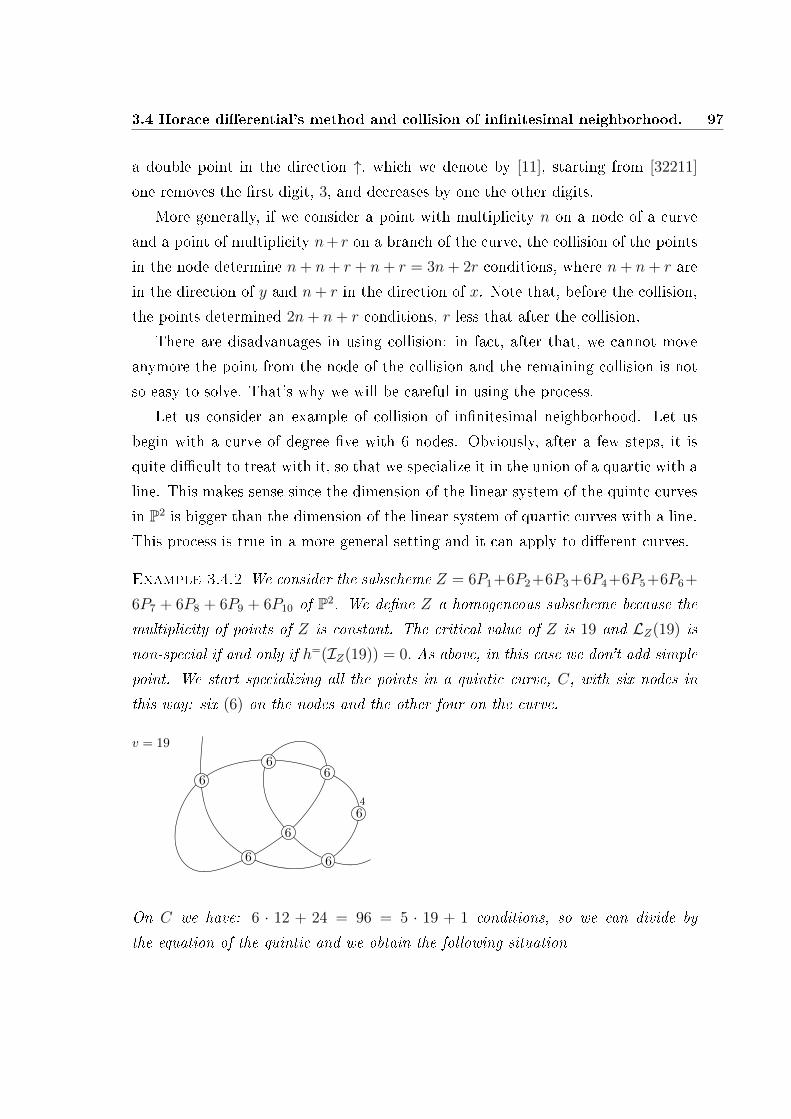
3.4 Horace dierential's method and collision of innitesimal neighborhood. 97
a double point in the direction ↑, which we denote by [11], starting from [32211]
one removes the rst digit, 3, and decreases by one the other digits.
More generally, if we consider a point with multiplicity n on a node of a curve
and a point of multiplicity n+ r on a branch of the curve, the collision of the points
in the node determine n+ n+ r + n+ r = 3n+ 2r conditions, where n+ n+ r are
in the direction of y and n+ r in the direction of x. Note that, before the collision,
the points determined 2n+ n+ r conditions, r less that after the collision.
There are disadvantages in using collision: in fact, after that, we cannot move
anymore the point from the node of the collision and the remaining collision is not
so easy to solve. That's why we will be careful in using the process.
Let us consider an example of collision of innitesimal neighborhood. Let us
begin with a curve of degree ve with 6 nodes. Obviously, after a few steps, it is
quite dicult to treat with it, so that we specialize it in the union of a quartic with a
line. This makes sense since the dimension of the linear system of the quintc curves
in P2 is bigger than the dimension of the linear system of quartic curves with a line.
This process is true in a more general setting and it can apply to dierent curves.
Example 3.4.2 We consider the subscheme Z = 6P1+6P2+6P3+6P4+6P5+6P6+
6P7 + 6P8 + 6P9 + 6P10 of P2. We dene Z a homogeneous subscheme because the
multiplicity of points of Z is constant. The critical value of Z is 19 and LZ(19) is
non-special if and only if h=(IZ(19)) = 0. As above, in this case we don't add simple
point. We start specializing all the points in a quintic curve, C, with six nodes in
this way: six (6) on the nodes and the other four on the curve.
6
66
6
6
6
6
4
v = 19
On C we have: 6 · 12 + 24 = 96 = 5 · 19 + 1 conditions, so we can divide by
the equation of the quintic and we obtain the following situation
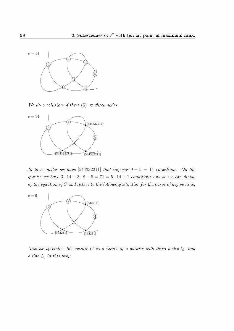
98 3. Subschemes of P2 with ten fat point of maximum rank.
4
4
54
v = 14
4
4
4 4
We do a collision of three (5) on three nodes.
4
4
5
v = 14
4
[544332211]
[544332211] [544332211]
In these nodes we have [544332211] that imposes 9 + 5 = 14 conditions. On the
quintic we have 3 · 14 + 3 · 8 + 5 = 71 = 5 · 14 + 1 conditions and so we can divide
by the equation of C and reduce to the following situation for the curve of degree nine.
2
2
4
v = 9
2
[332211]
[332211] [332211]
Now we specialize the quintic C in a union of a quartic with three nodes Q, and
a line L, in this way:
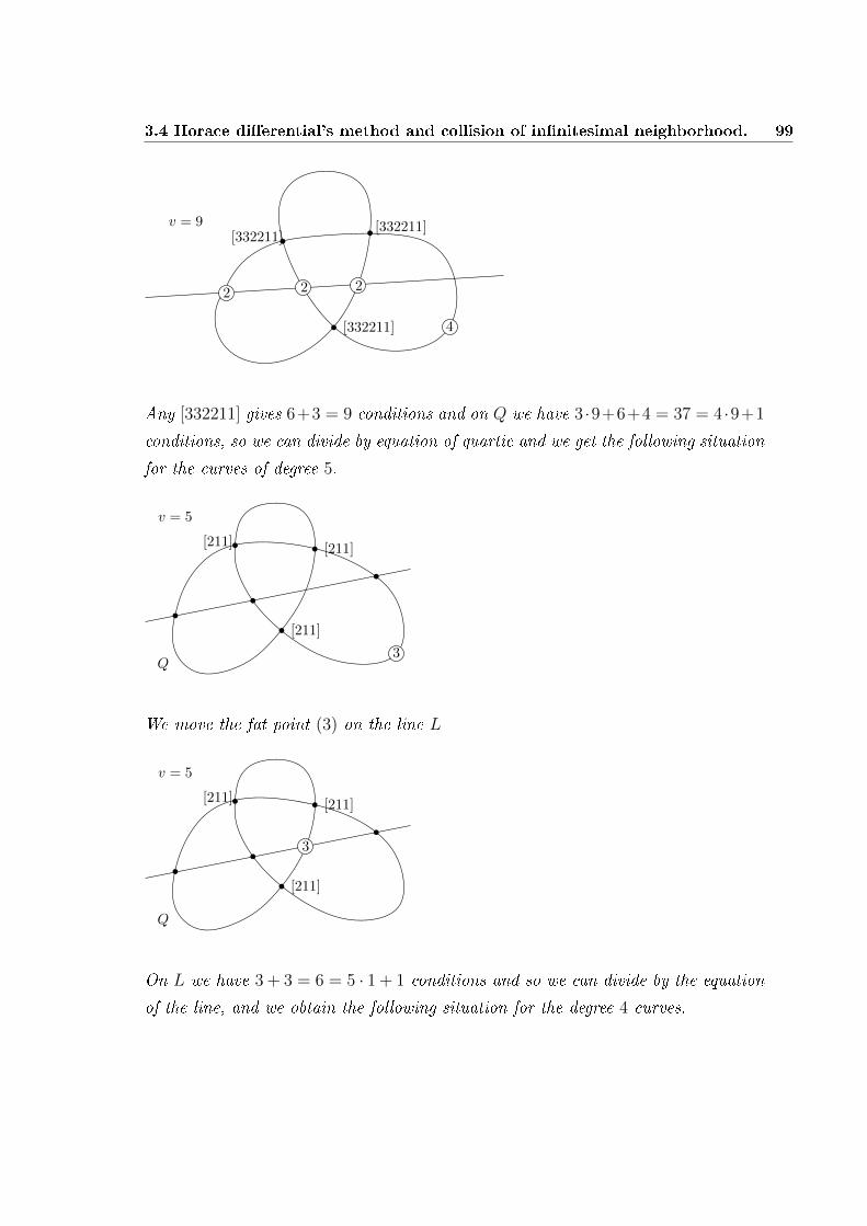
3.4 Horace dierential's method and collision of innitesimal neighborhood. 99
v = 9
2 2 2
4
[332211][332211]
[332211]
Any [332211] gives 6+3 = 9 conditions and on Q we have 3 ·9+6+4 = 37 = 4 ·9+1
conditions, so we can divide by equation of quartic and we get the following situation
for the curves of degree 5.
v = 5
Q
[211]
[211]
[211]
3
We move the fat point (3) on the line L
v = 5
Q
[211]
[211]
[211]
3
On L we have 3 + 3 = 6 = 5 · 1 + 1 conditions and so we can divide by the equation
of the line, and we obtain the following situation for the degree 4 curves.

100 3. Subschemes of P2 with ten fat point of maximum rank.
v = 4
Q
[211]
[211]
[211]
2
Any [211] gives 5 conditions so that, on a quartic, we have 3 · 5 + 2 = 17 = 4 · 4 + 1
conditions and we can divide by the equation of Q. In the end we obtain
v = 0
Since the remaining point is clearly not contained in a curve of degree zero, we
conclude that h0(IZ(19)) = 0 and thus LZ(19) is non-special.
3.5 Cremona transformations.
In this section we deal with Cremona transformations. We will use them in this
work in order to reduce more linear systems to only one, decreasing the number of
cases to study.
Cremona transformations act on the blow-up points. In other words, applying a
Cremona transformation is the same as changing the basis of Pic(S), where we
denote by S the P2 blown-up in the base points of the considered system. After a
Cremona transformation, the system seems to be dierent from the starting one,
even if it just seen in two dierent basis.
We recall some notation. Let Z = b1P1 + ...bkPk be a subscheme of P2 and
let p : S → P2 denote the blowing-up at the Pi's. Let Ei be the corresponding
exceptional curves. A bases of Pic(S) is given by ε = (l − E1 − ...− Ek) where l isthe class of line in P2; a such basis is also called an exceptional conguration.
If D ∈ IZ(v) where v is the critical value of Z then we can write D = (v; b1, ..., bk)
3.5 Cremona transformations. 101
in Pic(S).
Definition 3.5.1 As usual an exceptional curve (of the rst kind), E, is a curve
isomorphic to P1 with E2 = −1.
We will say that Σ =∑niEi is a bunch of disjoint exceptional curves if ni ≥ 0 for
all i, each Ei is an exceptional curve and Ei · Ej = 0 if i 6= j.
We have Pic(S) ' Zk+1 with the basis (l;−E1, ...,−EK) given by exceptional con-
guration ε. The intersection product denes a bilinear form on Pic(S). Let
r0 = l − E1 − E2 − E3, ri = Ei − Ei+1. Moreover associated to the ri's we have
the reections si : Pic(S) → Pic(S) dened by si(x) = x + (x · ri)ri. the si's
preserve the intersection product and x the canonical bundle of P2, K.
We are interested in s0 (Cremona transformation). We have:
s0(l) = 2l − E1 − E2 − E3,
s0(−E1) = E2 + E3 − l,s0(−E2) = E1 + E3 − l,s0(−E3) = E1 + E2 − l,s0(−Ei) = −Ei for i > 3.
If (v; b1, ..., bk) are the coordinates of D in the basis ε, then B′ = (s0(l); s0(−Ei))is a basis of Pic(S) and the coordinates of D in this basis are (v′; ci) where:
v′ = 2v − b1 − b2 − b′3,c1 = v − b2 − b3,
c2 = v − b1 − b3,
c3 = v − b1 − b2,
ci = bi for i > 3.
If the points Pi are distinct and in general position, the basis B′ corresponds
to an exceptional conguration ε′ = (l′;−E ′1, ...,−E ′k); moreover the corresponding
points, obtained by blowing down, Pi are again distinct and in general position.
Finally we observe that : v′ < v if and only if a < b1 + b2 + b3.
Of course if b1 ≥ b2 ≥ ... ≥ b9 then c1 ≥ c2 ≥ c3 but it could be that c3 < c4.
We show an example
Example 3.5.2 Let D = (17; 8, 6, 6, 5, 5, 5, 5, 4, 4, 4) be a divisor in Pic(S), we ap-
ply to D the Cremona transformation. The new coordinates of D are (v′, ci) where:
102 3. Subschemes of P2 with ten fat point of maximum rank.
v′ = 34− 8− 6− 6 = 14,
c1 = 17− 6− 6 = 5,
c2 = 17− 8− 6 = 3,
c3 = 17− 8− 6 = 3,
ci = bi for i > 3.
After the transformations, it occurs that D′ = (14; 5, 5, 5, 5, 5, 4, 4, 4, 3, 3), since
2v−c1−c2−c3 = 28−15 = 13 < 14, we can apply again the Cremona transformation
to D′. We obtain D′′ = (13; 5, 5, 4, 4, 4, 4, 4, 4, 3, 3) and another time we apply the
transformation. In the end we have
D′′′ = (12; 4, 4, 4, 4, 4, 4, 4, 3, 3, 3) and we stop the transformation process because
2v − c1 − c2 − c3 = 12 = v.
3.6 Subschemes of P2 with ten fat points of multi-
plicity less than nine.
In this section we get to the heart of the matter focusing our attention on particular
subschemes Z = b1P1+...+b10P10 of P2 for which exists almost a point of multiplicity
like 8 so that 4 ≤ bi ≤ 8for all i.
We don't consider the subscheme with a point of multiplicity minor than 4 be-
cause the associated linear system veries the conjecture of Harbourne-Hirschowitz.
Let's begin with the studying of he rst cases. Taken ten general points P1, ..., P10
we consider the subscheme Z = 8P1 +4P2 +4P3 + ...+4P10, In order to make it easy,
we indicate Z with the list (8, 4, 4, 4, 4, 4, 4, 4, 4, 4, ). The critical value of Z is 15
and we denote with x := h0(OP2(v))− h0(OZ(v)), this number indicates the dimen-
sion which LZ(v) need to have in order to be non-special and it also represents the
number of the simple points to have add to subscheme Z in order to start with Ho-
race's method. In this case x = 10. Considering now Z1 = (8, 5, 4, 4, 4, 4, 4, 4, 4, 4)
and Z2 = (8, 5, 5, 4, 4, 4, 4, 4, 4, 4), they have critical value equal 15 and respec-
tively x equal 5 and 0. By the proposition 3.3.1, if Z2 is non-special then Z1 e
Z are non-special too, afterwards lets analyze the case Z2. Before starting with
the Horace's method, we apply the Cremona's transformation s0 to Z2, we get
3.6 Subschemes of P2 with ten fat points of multiplicity less than nine. 103
s0((15; 8, 5, 5, 4, 4, 4, 4, 4, 4, 4)) = (6; 2, 2, 2, 2, 2, 2, 2, 2, 2, 1) which is a system, where
the conjecture of Harbourne-Hirschowitz holds.
This proceeding bring us to a reduction of several cases, that we list below:
Z1 = (2, 2, 2, 2, 2, 2, 2, 2, 2, 1) v = 6 x = 0
Z2 = (4, 3, 3, 3, 3, 3, 3, 3, 3, 3) v = 10 x = 2
Z3 = (5, 4, 4, 4, 4, 4, 4, 4, 4, 4) v = 13 x = 0
Z4 = (3, 3, 3, 3, 3, 3, 3, 3, 2, 2) v = 9 x = 1
Z5 = (5, 4, 4, 4, 4, 4, 4, 4, 4, 3) v = 13 x = 4
Z6 = (4, 4, 4, 4, 4, 4, 4, 3, 3, 3) v = 12 x = 3
Z7 = (5, 5, 5, 5, 5, 5, 5, 5, 5, 5) v = 16 x = 0
Z8 = (6, 5, 5, 5, 5, 5, 5, 5, 5, 4) v = 16 x = 2
Z9 = (6, 6, 6, 6, 6, 6, 6, 6, 6, 6) v = 19 x = 0
Z10 = (4, 4, 4, 4, 4, 4, 4, 4, 3, 1) v = 12 x = 4
Z11 = (4, 4, 4, 4, 4, 4, 4, 4, 3, 2) v = 12 x = 2
Z12 = (5, 5, 5, 5, 5, 5, 5, 5, 4, 3) v = 15 x = 0
Z13 = (7, 6, 6, 6, 6, 6, 6, 6, 5, 5) v = 19 x = 5
Z14 = (3, 3, 3, 3, 3, 3, 3, 2, 2, 2) v = 9 x = 4
Z15 = (6, 6, 6, 6, 6, 6, 5, 5, 5, 5) v = 18 x = 4
Z16 = (6, 6, 6, 6, 6, 6, 6, 5, 5, 4) v = 18 x = 3
Z17 = (7, 6, 6, 6, 6, 6, 6, 6, 6, 4) v = 19 x = 4
Z18 = (8, 7, 7, 7, 7, 7, 7, 7, 6, 6) v = 22 x = 2
Z19 = (8, 7, 7, 7, 7, 7, 7, 7, 7, 5) v = 22 x = 1
Z20 = (4, 4, 4, 4, 4, 4, 4, 4, 4, 0) v = 12 x = 1
Z21 = (5, 5, 5, 5, 5, 5, 5, 5, 4, 2) v = 15 x = 3
Z22 = (3, 3, 3, 3, 3, 3, 3, 3, 2, 1) v = 9 x = 3
Z23 = (7, 7, 7, 7, 7, 7, 6, 6, 6, 6) v = 21 x = 1
Z24 = (7, 7, 7, 7, 7, 7, 7, 6, 6, 5) v = 21 x = 0
Z25 = (2, 2, 2, 2, 2, 2, 2, 2, 2, 0) v = 6 x = 1
Z26 = (4, 4, 4, 4, 4, 4, 4, 4, 4, 4) v = 13 x = 5
Z27 = (6, 6, 6, 6, 6, 6, 6, 6, 4, 4) v = 18 x = 2
Z28 = (1, 1, 1, 1, 1, 1, 1, 1, 1, 0) v = 3 x = 1
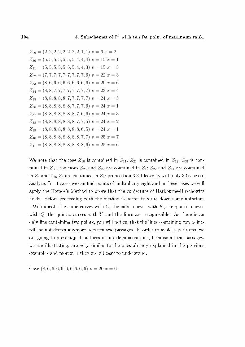
104 3. Subschemes of P2 with ten fat point of maximum rank.
Z29 = (2, 2, 2, 2, 2, 2, 2, 2, 1, 1) v = 6 x = 2
Z30 = (5, 5, 5, 5, 5, 5, 5, 4, 4, 4) v = 15 x = 1
Z31 = (5, 5, 5, 5, 5, 5, 5, 4, 4, 3) v = 15 x = 5
Z32 = (7, 7, 7, 7, 7, 7, 7, 7, 7, 6) v = 22 x = 3
Z33 = (8, 6, 6, 6, 6, 6, 6, 6, 6, 6) v = 20 x = 6
Z34 = (8, 8, 7, 7, 7, 7, 7, 7, 7, 7) v = 23 x = 4
Z35 = (8, 8, 8, 8, 8, 7, 7, 7, 7, 7) v = 24 x = 5
Z36 = (8, 8, 8, 8, 8, 8, 7, 7, 7, 6) v = 24 x = 1
Z37 = (8, 8, 8, 8, 8, 8, 8, 7, 6, 6) v = 24 x = 3
Z38 = (8, 8, 8, 8, 8, 8, 8, 7, 7, 5) v = 24 x = 2
Z39 = (8, 8, 8, 8, 8, 8, 8, 8, 6, 5) v = 24 x = 1
Z40 = (8, 8, 8, 8, 8, 8, 8, 8, 7, 7) v = 25 x = 7
Z41 = (8, 8, 8, 8, 8, 8, 8, 8, 8, 6) v = 25 x = 6
We note that the case Z10 is contained in Z11; Z21 is contained in Z12; Z31 is con-
tained in Z30; the cases Z25 and Z29 are contained in Z1; Z22 and Z14 are contained
in Z4 and Z26,Z5 are contained in Z3; proposition 3.3.1 leave us with only 32 cases to
analyze. In 11 cases we can nd points of multiplicity eight and in these cases we will
apply the Horace's Method to prove that the conjecture of Harbourne-Hirschowitz
holds. Before proceeding with the method is better to write down some notations
. We indicate the conic curves with C, the cubic curves with K, the quartic curves
with Q, the quintic curves with Y and the lines are recognizable. As there is an
only line containing two points, you will notice, that the lines containing two points
will be not drown anymore between two passages. In order to avoid repetitions, we
are going to present just pictures in our demonstrations, because all the passages,
we are illustrating, are very similar to the ones already explained in the previous
examples and moreover they are all easy to understand.
Case (8, 6, 6, 6, 6, 6, 6, 6, 6, 6) v = 20 x = 6.

3.6 Subschemes of P2 with ten fat points of multiplicity less than nine. 105
6
6
6
8
66
We divide by eq. of Q
5v = 20
Q
4
7
56
5
v = 16
4
4
Q
4
7
55
4
v = 16
14
[544332211]
3
2
We divide by eq. of Q
Q
2
6
45
9
[332211]
2
v = 122
Q
v = 12
4 2
69
[332211]
L
4
2
2 We divide by eq. of cubic
4
K
v = 9
55 3
[211]
4
L
4 4
K
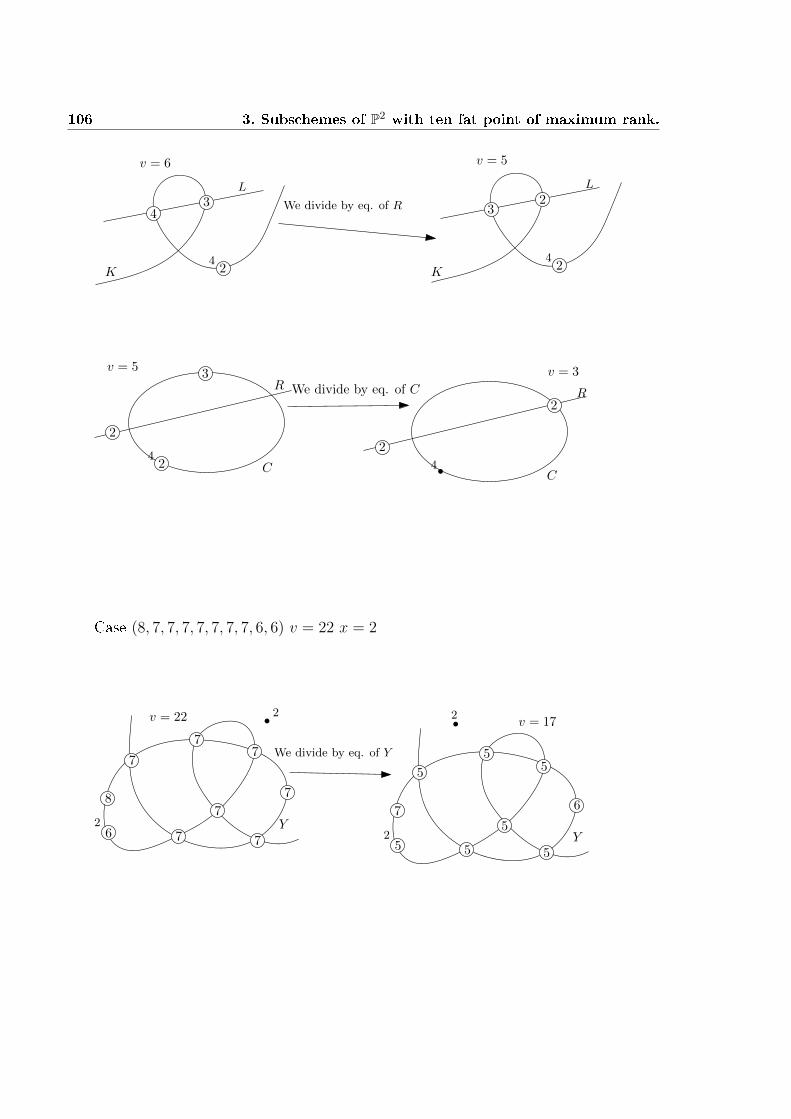
106 3. Subschemes of P2 with ten fat point of maximum rank.
v = 6
24
34
We divide by eq. of R
v = 5
24
L
32
K K
L
24
3v = 5
We divide by eq. of CR
C 4
2
v = 3
2R
C
2
Case (8, 7, 7, 7, 7, 7, 7, 7, 6, 6) v = 22 x = 2
7
v = 22
77
7
77
7
8
6
2
2
We divide by eq. of Y
Y
67
5
2
2
v = 17
5
5
5
55
5
Y
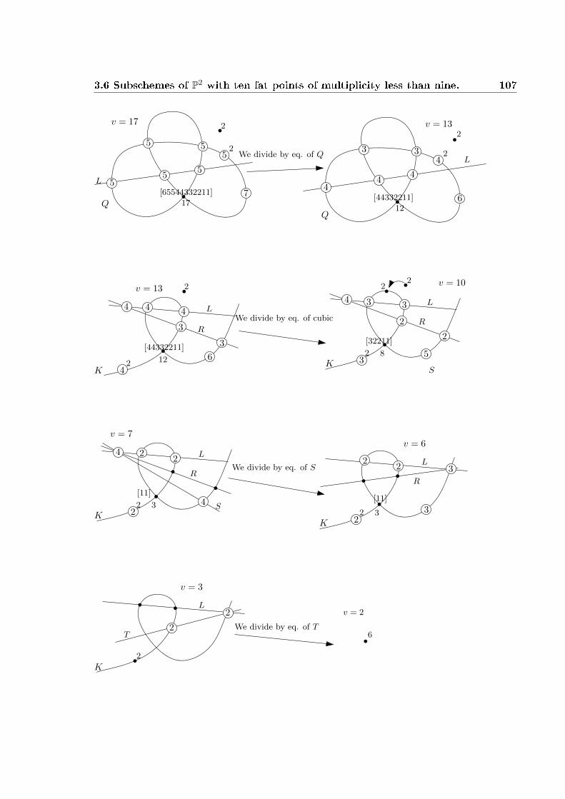
3.6 Subschemes of P2 with ten fat points of multiplicity less than nine. 107
5
5
7
v = 17
5
55
5
17
[65544332211]
We divide by eq. of Q2
Q
L
2
4
6
L
12
[44332211]
v = 13
44
4
33
2
2
Q
v = 13
4 4 4
3
3
4
612
[44332211]
We divide by eq. of cubicL
R
8
[32211]
3 3
2
2
L
R
4
53
S
2
2
2
2
v = 102
KK
3
[11]
L
R
22
v = 7
224
4 S
We divide by eq. of S
K 3
L
R
22
22
3[11]
3
v = 6
K
L
2
v = 3
2
2
TWe divide by eq. of T
6
v = 2
K
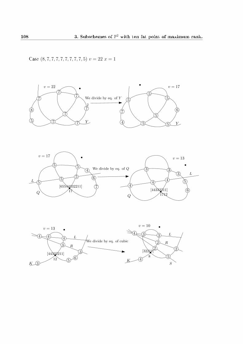
108 3. Subschemes of P2 with ten fat point of maximum rank.
Case (8, 7, 7, 7, 7, 7, 7, 7, 7, 5) v = 22 x = 1
72
v = 22
77
7
77
7
8
5
We divide by eq. of Y
Y
67
4
v = 17
55
5
5
5 5 Y
5
4
7
v = 17
6
5
L 55
5
17
[65544332211]
We divide by eq. of Q
Q
3
6
5
L
1712
[44332211]
v = 13
44
4
33
Q
5
v = 13
4 4 4
3
3
3
612
[44332211]
We divide by eq. of cubicL
R
v = 10
8
[32211]
3 3
2
2
L
R
4
54
2
SKK

3.6 Subschemes of P2 with ten fat points of multiplicity less than nine. 109
v = 9
8
[32211]
3 3
2
2
L
R
3
44
S
We divide by eq. of cubic
v = 6
3
[11]
L
R
3
3
2 2
3K K
v = 5
3
[11]
L
R
33
2
We divide by the eq. of cubic
v = 2
22K
K
v = 4
[11]
L
R
2
2
2
3S
We divide by eq. of S
K
[11]
R
2
3
v = 3
K
2
Case (8, 8, 7, 7, 7, 7, 7, 7, 7, 7) v = 23 x = 4
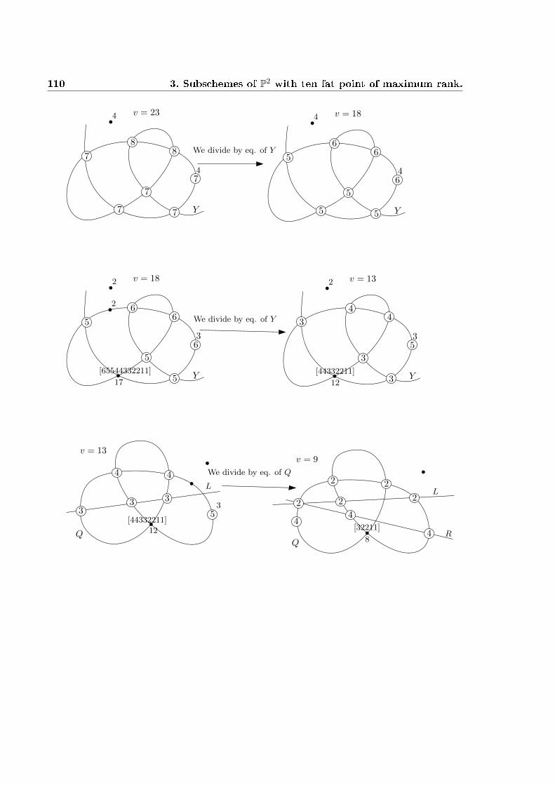
110 3. Subschemes of P2 with ten fat point of maximum rank.
74
7
77
7
Y
v = 23
88
4
We divide by eq. of Y
64
5
55
5
Y
v = 18
66
4
63
5
5
5
Y
v = 18
66
2
2
[65544332211]
17
We divide by eq. of Y
53
3
3 Y
v = 132
[44332211]
12
44
3
v = 13
L
3
12
[44332211]
Q
44
533 3
We divide by eq. of Q
v = 9
L
8
[32211]
Q
2 2
R
2 2 2
4
44

3.6 Subschemes of P2 with ten fat points of multiplicity less than nine. 111
v = 8
4K
2 2
T2
2L
R3 3
8
[32211]
We divide by eq. of K
v = 5
3K
2
T
2 2
3
[11]
2
v = 2
2K
L
2
In the end, dividing by the equation of the line L, we rest with v = 1 and three
simple point. Absurd.
Case (8, 8, 8, 8, 8, 7, 7, 7, 7, 7) v = 24 x = 5
8
7
7
8
8
8
7
8
Y
v = 24 5
3
We divide by eq. of Y
5
65
7
Y
v = 19 5
3
6
6
6
6
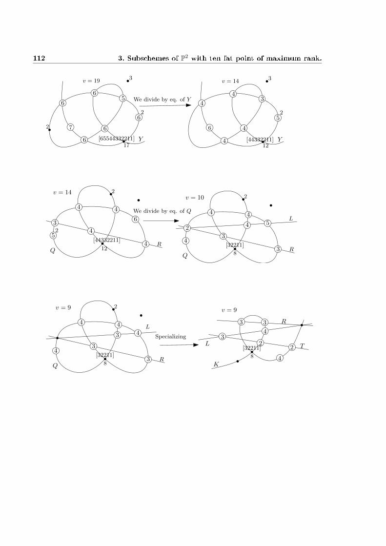
112 3. Subschemes of P2 with ten fat point of maximum rank.
65
7
Y
v = 19 3
6
6
6
62
2
17[65544332211]
We divide by eq. of Y4
3
6
Y
v = 14 3
52
12
4
4
4 [44332211]
v = 14
Q
4 4
R
36
4
45
12
[44332211]
2
2
We divide by eq. of Q
v = 10
Q
4 4
R3
34
2
8
[32211]
L
254
v = 9
Q
4 4
R3
34
2
8
[32211]
43 Specializing
L
v = 9
4K
T22
3
3
4
3 R
L
8
[32211]

3.6 Subschemes of P2 with ten fat points of multiplicity less than nine. 113
v = 6
3K
3
3
[11]
3
2
T
2
Specializing
3
3
22
2
v = 6T
R
T
3
2
2
2
v = 4
3
C
We divide by eq. of C
2v = 2
C
2
Case (8, 8, 8, 8, 8, 8, 7, 7, 7, 6) v = 24 x = 1
7
77
v = 24
8
88
882
6
4
We divide by eq. of Y
Y5
2
4v = 19
6
66
6
6
7
5 5 Y
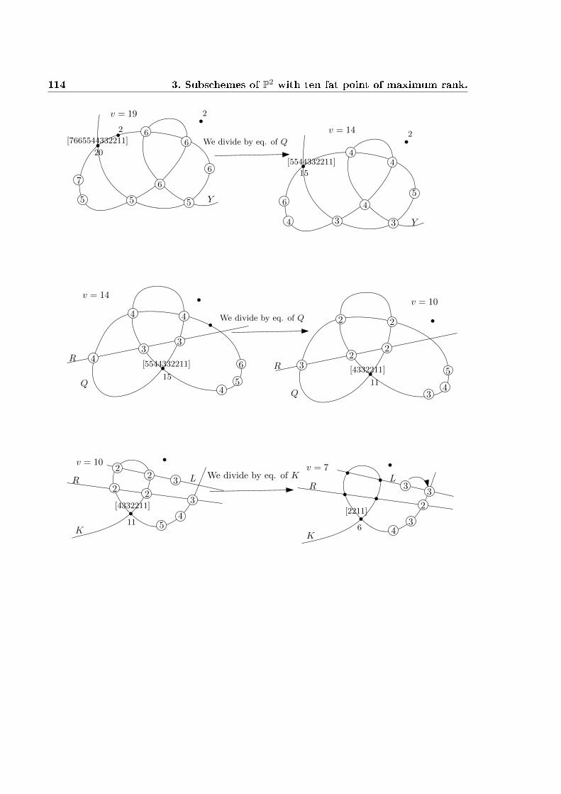
114 3. Subschemes of P2 with ten fat point of maximum rank.
5
2
66
6
6
7
5 5
v = 19
2
20
[7665544332211] We divide by eq. of Q
Y
3
2
4
15
[5544332211]
v = 14
44
4
65
3 Y
v = 14
6
45
44
15
[5544332211]
We divide by eq. of Q
43
3
Q
R
4
3
11
[4332211]
v = 10
2
3
22
5
2
Q
R
5
v = 10
3
4
32
2
11
[4332211]
We divide by eq. of K
22
K
R Lv = 7
3
6
[2211]
43
2
3
K
RL
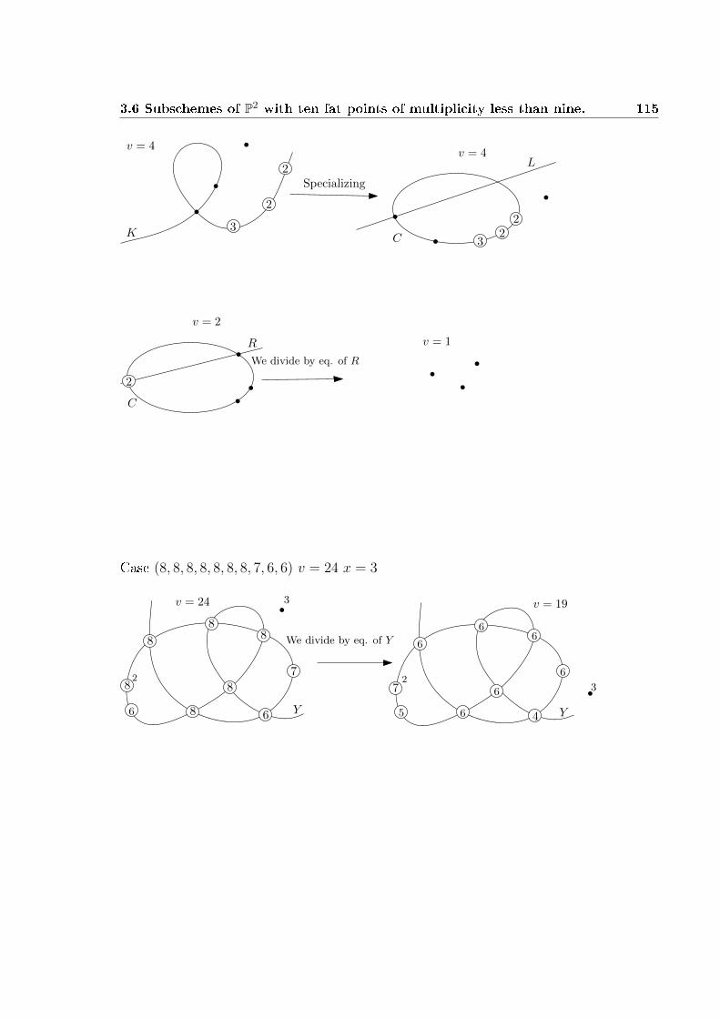
3.6 Subschemes of P2 with ten fat points of multiplicity less than nine. 115
v = 4
3
2
2
Specializing
K3
22
v = 4L
C
v = 2
C
R
2
We divide by eq. of R
v = 1
Case (8, 8, 8, 8, 8, 8, 8, 7, 6, 6) v = 24 x = 3
7
68
v = 24
8
88
882
6
We divide by eq. of Y
3
Y4
2
5
v = 19
37
6
6
6
6
6
6 Y
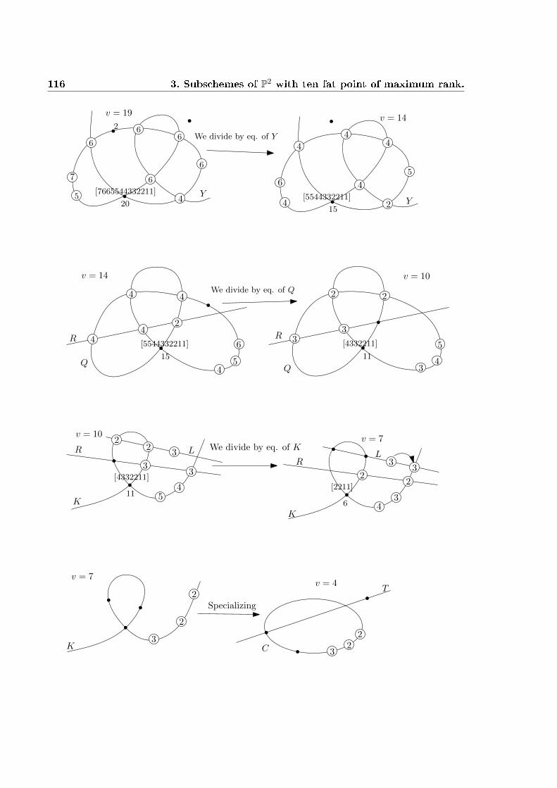
116 3. Subschemes of P2 with ten fat point of maximum rank.
45
7
6
6
6
6
6
v = 19
2
20
[7665544332211]
We divide by eq. of Y
Y2
6
15
[5544332211]
v = 14
4
44
4
4
5
Y
v = 14
6
45
44
44
2
15
[5544332211]
We divide by eq. of Q
Q
R
4
3
11
[4332211]
v = 10
3
3
22
5
Q
R
5
v = 10
33
4
32
2
11
[4332211]
We divide by eq. of KR L
K
v = 7
2
3
6
[2211]
43
2
3R
L
K
v = 7
3
2
2
Specializing
K3
22
v = 4T
C

3.6 Subschemes of P2 with ten fat points of multiplicity less than nine. 117
v = 2
C
R
2
We divide by eq. of R
v = 1
Case (8, 8, 8, 8, 8, 8, 8, 7, 7, 5) v = 24 x = 2
v = 24
7 7
5
886
2
We divide by eq. of Q
Q
5
4
676
2
v = 20
5
Q
5
4
673
2v = 20
5
R
77
7
We divide by eq. of R
Q
5
4
673
2
v = 19
5
R66
6
Q
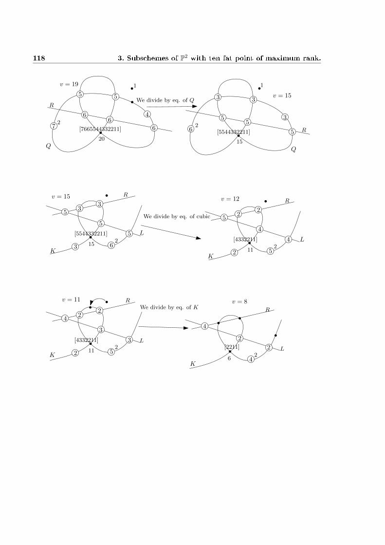
118 3. Subschemes of P2 with ten fat point of maximum rank.
5
4
72
1v = 19
5
R
66
6
20
[7665544332211]
We divide by eq. of Q
Q
3
32
1
v = 153
R
5
15
[5544332211]65
5
Q
62
v = 15
33
5
5
5
3 15
[5544332211]
We divide by eq. of cubic
52
22
5
4
4
2 11
[4332211]
v = 12
KK
RR
LL
52
22
4
3
3
2 11
[4332211]
v = 11We divide by eq. of K
L
R
K42
4
6
[2211]
v = 8
2
2 L
R
K

3.6 Subschemes of P2 with ten fat points of multiplicity less than nine. 119
4
6
[2211]
v = 8
2
2
S
4
4
We divide by eq. of S
K
L
R
4
6
[2211]
v = 7
2
23
3 K
L
3
6
[2211]
v = 6
3
3
3
We divide by eq. of K
L
K
v = 3
2
2
2
K
2
22
v = 3
We divide by eq. of C
C
R
v = 1
Case (8, 8, 8, 8, 8, 8, 8, 8, 6, 5) v = 24 x = 1
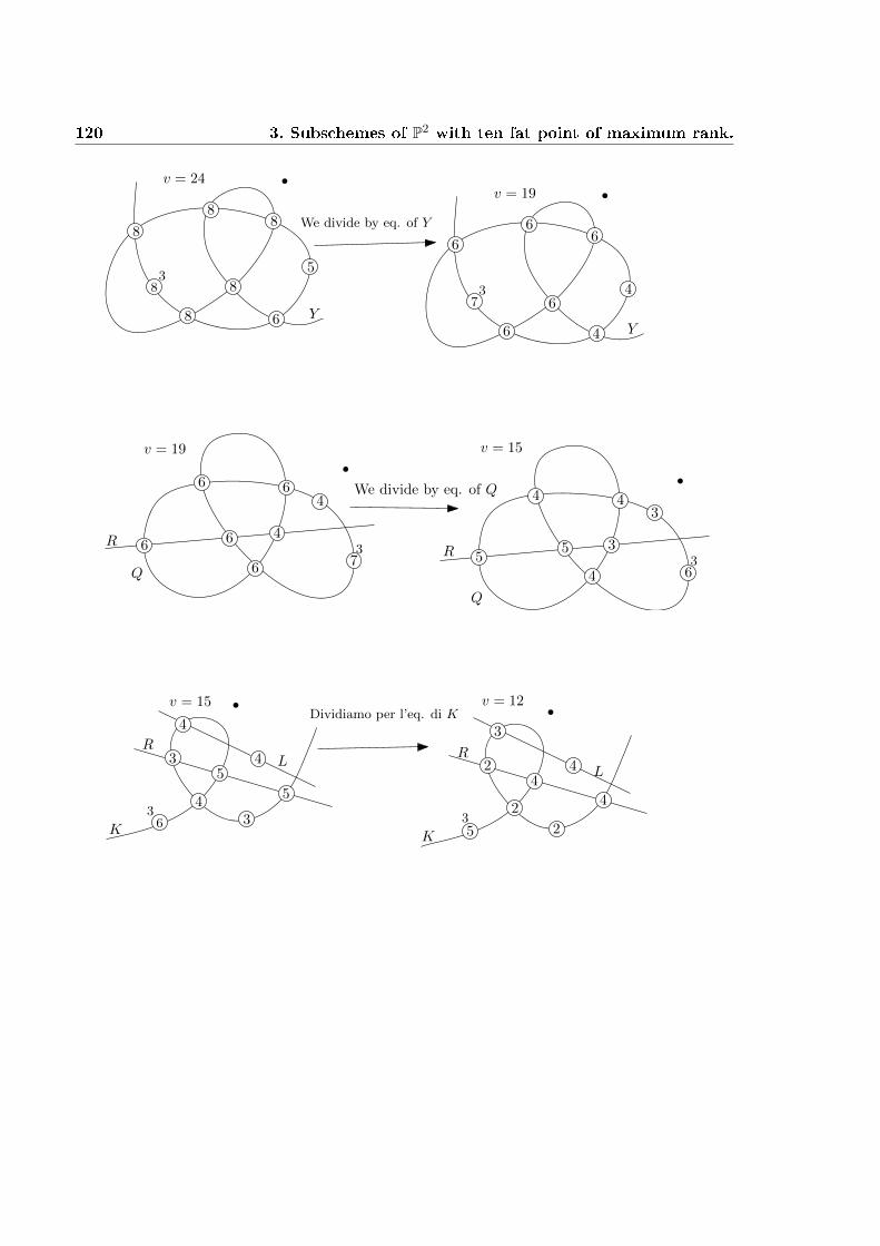
120 3. Subschemes of P2 with ten fat point of maximum rank.
8
5
v = 24
6
8
8
8
8
83
We divide by eq. of Y
Y
v = 19
4
73
6
66
6
6
4
Y
6
66
4
6 6 4
73
v = 19
We divide by eq. of Q
Q
R
3
53
63
v = 15
44
4
5
Q
R
3
v = 15
4
4
54
53
63
Dividiamo per l’eq. di K
R
K
L
v = 12
4
3
2
35
4
2
2
4
R
K
L
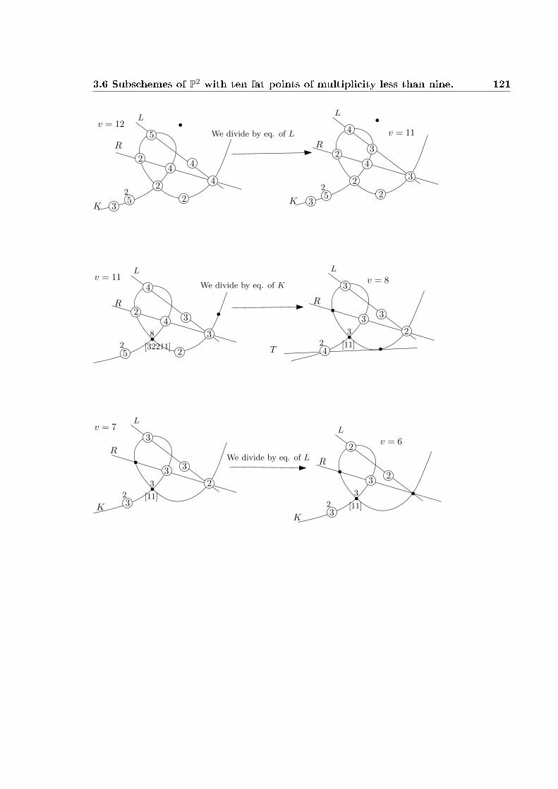
3.6 Subschemes of P2 with ten fat points of multiplicity less than nine. 121
v = 12
42
25
4
2
23
4
5 We divide by eq. of L
L
K
R
v = 11
2
25
4
2
23
L
4
3
3
K
R
v = 11
2
25
4
2
L
4
38
[32211]
We divide by eq. of K
3
R
v = 8L
3
[11]
3
3
3
224
R
T
v = 7L
3
[11]
3
3
3
223
We divide by eq. of LR
K
v = 6L
3
[11]
23
23
2
R
K
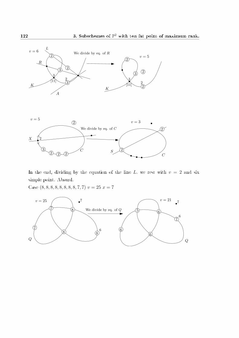
122 3. Subschemes of P2 with ten fat point of maximum rank.
v = 6L
3
[11]
23
2
23
We divide by eq. of R
R
A
K
v = 5
3
[11]
23
2
22
K
v = 5
32 2 2
2
We divide by eq. of C
X
2 v = 3
2
2
SCC
In the end, dividing by the equation of the line L, we rest with v = 2 and six
simple point. Absurd.
Case (8, 8, 8, 8, 8, 8, 8, 8, 7, 7) v = 25 x = 7
v = 25
7 8
78
We divide by eq. of Q
Q
7
86
v = 21
5 6
7
6
6
7
6
Q
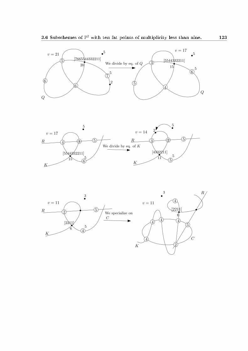
3.6 Subschemes of P2 with ten fat points of multiplicity less than nine. 123
v = 21
5
5
66
2
20
[7665544332211]We divide by eq. of Q
Q
57
v = 175
5
4
15
[5544332211]
6
5
3
Q
3
6
v = 17
15
[5544332211]
5
4 5
We divide by eq. of K
5
K
R 2
5
v = 14
11
[4332211]
5
53
5
2
K
R
5
v = 11
6
[2211]
3
5
4
2R
K
We specialize on
C
v = 11
6
[2211]
44 4
4
4
5
2
3 R
K
C
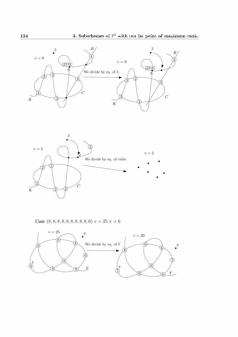
124 3. Subschemes of P2 with ten fat point of maximum rank.
v = 9
R
6
[2211]
3
4
43 3
We divide by eq. of L
3
3
C
K
v = 8
R
6
[2211]
3
3 3
3
3
3
3C
K
v = 5
2
2
22
2
2
We divide by eq. of cubic
v = 2
CK
2
2
Case (8, 8, 8, 8, 8, 8, 8, 8, 8, 6) v = 25 x = 6
6
88 8
8
88
8
3
We divide by eq. of Y
Y
6v = 25
5
73
66
6
6
6
6
6 Y
v = 20

3.6 Subschemes of P2 with ten fat points of multiplicity less than nine. 125
5
72
4
v = 20
66
6
6
6
2
20
[7665544332211]
We divide by eq. of Y
Y
4
62
4
v = 15
15
[5544332211]
4
44
4
4
Y
v = 15
4
4
4
46
6
44
4
15
[5544332211]
LWe divide by eq. of R
Q
R
v = 14
4
4
4
35
5
44
4
15
[5544332211]
Q
R
L
v = 10
2
3
2
11
[4332211]
L
44
32
3
3
Q
R
6
[2211]
L
v = 6
33
22
2
Q
R
We divide by eq. of Q
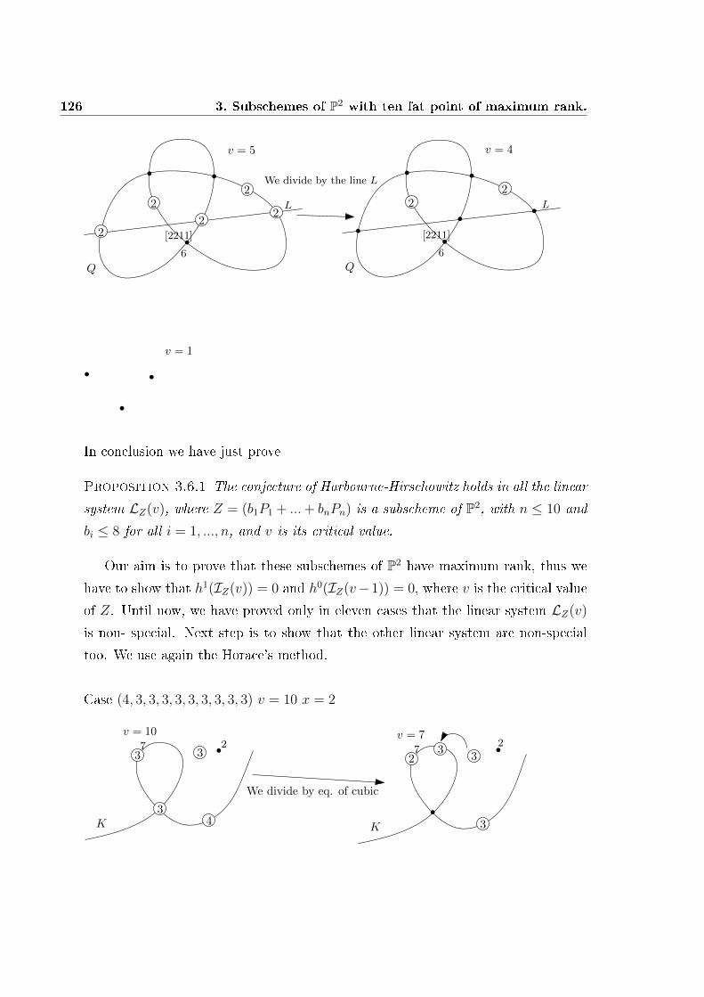
126 3. Subschemes of P2 with ten fat point of maximum rank.
6
[2211]
L
v = 5
22
22
2
Q
We divide by the line L
6
[2211]
L
v = 4
22
Q
v = 1
In conclusion we have just prove
Proposition 3.6.1 The conjecture of Harbourne-Hirschowitz holds in all the linear
system LZ(v), where Z = (b1P1 + ...+ bnPn) is a subscheme of P2, with n ≤ 10 and
bi ≤ 8 for all i = 1, ..., n, and v is its critical value.
Our aim is to prove that these subschemes of P2 have maximum rank, thus we
have to show that h1(IZ(v)) = 0 and h0(IZ(v−1)) = 0, where v is the critical value
of Z. Until now, we have proved only in eleven cases that the linear system LZ(v)
is non- special. Next step is to show that the other linear system are non-special
too. We use again the Horace's method.
Case (4, 3, 3, 3, 3, 3, 3, 3, 3, 3) v = 10 x = 2
v = 10
4
3
K3
37
We divide by eq. of cubic
2v = 7
3
2
K
37
23
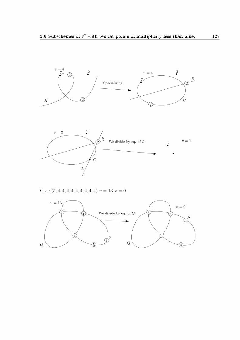
3.6 Subschemes of P2 with ten fat points of multiplicity less than nine. 127
v = 4
2K
7 22
Specializing
C
v = 4
7
2
2R
2
C
v = 2
R
2
2
L
We divide by eq. of L 2v = 1
Case (5, 4, 4, 4, 4, 4, 4, 4, 4, 4) v = 13 x = 0
Q 5
4 4
4
v = 13
We divide by eq. of Q
46
36
4
3 3
3
Q
v = 9
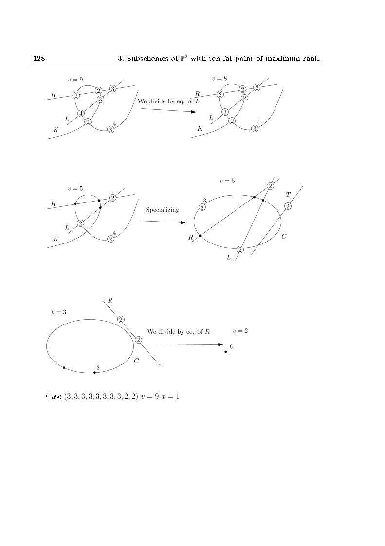
128 3. Subschemes of P2 with ten fat point of maximum rank.
v = 9
K2
3
4
22
3
34
R
L
We divide by eq. of L
v = 8
K2
2
3
22
2
34
R
L
v = 5
K
2
24
R
L2
Specializing
CR
L
T
2
2
223
v = 5
R
We divide by eq. of R
2
2
v = 3
C3
6
v = 2
Case (3, 3, 3, 3, 3, 3, 3, 3, 2, 2) v = 9 x = 1
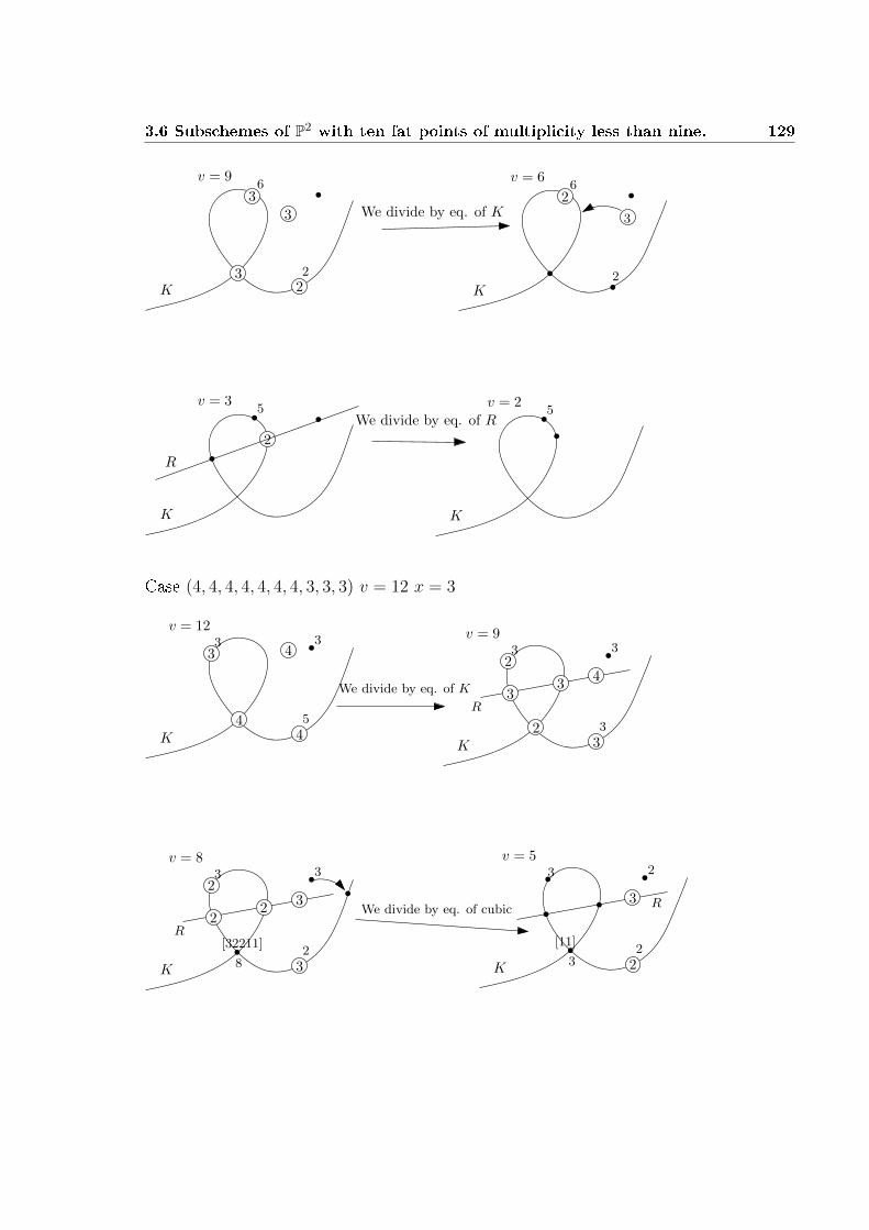
3.6 Subschemes of P2 with ten fat points of multiplicity less than nine. 129
v = 9
2K
3
3
6
3
2
v = 6
K
26
3
2
We divide by eq. of K
v = 3
K
5
2
R
We divide by eq. of R
v = 2
K
5
Case (4, 4, 4, 4, 4, 4, 4, 3, 3, 3) v = 12 x = 3
v = 12
4
3
K4
43 3
5
We divide by eq. of K
v = 9
3
2
K2
3 3
3
R3
34
v = 8
3
2
K
3 3
2
R2
23
8
[32211]
v = 5
2K
3 2
2
3
3
[11]
We divide by eq. of cubic R

130 3. Subschemes of P2 with ten fat point of maximum rank.
v = 5
2K
3
2
R
3
[11]
3 We divide by eq. of cubic
v = 2
K2
2 L
In the end, dividing by the equation of the line L, we rest with v = 1 and three
simple point. Absurd.
Case (5, 5, 5, 5, 5, 5, 5, 5, 5, 5) v = 16 x = 0
Q
5 5
557
3v = 16
We divide by eq. of Q
v = 12
Q
3
47
3
3
3
Q
3
46
3
11
[4332211]
2
v = 12
Q
36
6
[2211]
v = 8We divide by eq. of Q
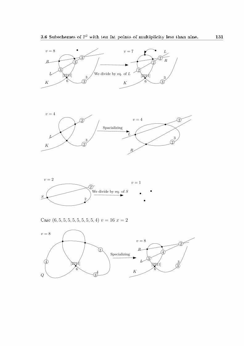
3.6 Subschemes of P2 with ten fat points of multiplicity less than nine. 131
3K
v = 8
3
R
L
33
3
6
[2211]
3K
v = 7
3
22
2
6
[2211]
L
R
We divide by eq. of L
2K
v = 4
3L
2
Spacializing
L
R
v = 4
23
2
v = 2
2
2
S
We divide by eq. of S
v = 1
Case (6, 5, 5, 5, 5, 5, 5, 5, 5, 4) v = 16 x = 2
v = 8
2
Q 3
4
6
[2211]
4
Specializing
K
v = 8
3
33
4
2
6
[2211]
R
L
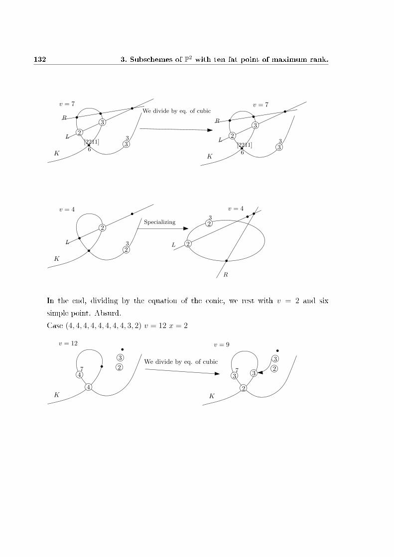
132 3. Subschemes of P2 with ten fat point of maximum rank.
K
v = 7
2
33
3
6
[2211]
R
L
We divide by eq. of cubic
K
2
33
3
6
[2211]
R
L
v = 7
K
v = 4
23
2
L
Specializing
L
R
2
23
v = 4
In the end, dividing by the equation of the conic, we rest with v = 2 and six
simple point. Absurd.
Case (4, 4, 4, 4, 4, 4, 4, 4, 3, 2) v = 12 x = 2
v = 12
K
4
4
3
7 2We divide by eq. of cubic
v = 9
K
3
2
3
7 23
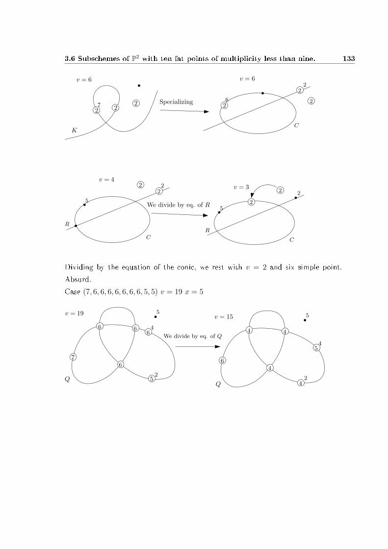
3.6 Subschemes of P2 with ten fat points of multiplicity less than nine. 133
v = 6
K
27 2
2Specializing
22
26
v = 6
2
C
2
v = 4
5
2
C
R
We divide by eq. of R
2
2v = 3
5
2
2
R
C
Dividing by the equation of the conic, we rest with v = 2 and six simple point.
Absurd.
Case (7, 6, 6, 6, 6, 6, 6, 6, 5, 5) v = 19 x = 5
v = 19
Q 5
5
7
2
66
6
We divide by eq. of Q64
v = 15 5
6
2
4
54
4 4
4Q
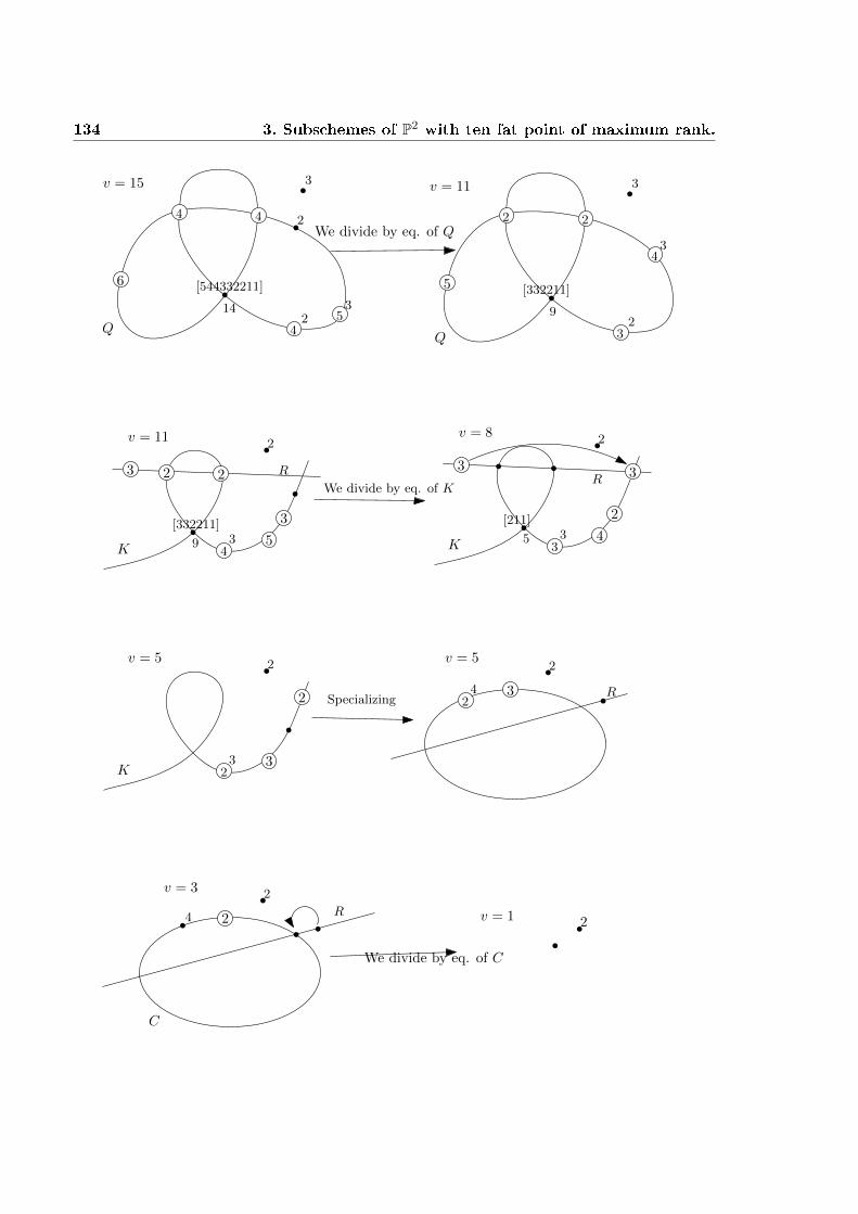
134 3. Subschemes of P2 with ten fat point of maximum rank.
v = 15
Q
3
6
2
4 4
4
14
[544332211]
We divide by eq. of Q2
53
v = 11 3
5
2
43
2 2
3
9
[332211]
Q
v = 11
K
2
5
2 23
3
439
[332211]
We divide by eq. of K
R
v = 8
K
2
4
3
2
335
[211]
3R
v = 5
K
2
323
2 Specializing3
24
2v = 5
R
R24
2v = 3
C
We divide by eq. of C
2v = 1

3.6 Subschemes of P2 with ten fat points of multiplicity less than nine. 135
Case (6, 6, 6, 6, 6, 6, 5, 5, 5, 5) v = 18 x = 4
6
5
4
64
6
Q
53 We divide by eq. of Q
and we collapse a node
v = 18
4
54
4
Q
242
11
[4332211]
v = 14 2
2
2
44
2
Q
32
6
[2211]
Specializing
v = 10
K6
[2211]
v = 10 2
R
L
223
3
4
4
42
K6
[2211]
v = 9
R
L
222
3
3
3
42
We divide by eq. of K
K
v = 6
R
L
2
2
2
2
32

136 3. Subschemes of P2 with ten fat point of maximum rank.
T2
2
2
2
32
C
We divide by eq. of C
R
L
v = 6 2
2
22
C
2
v = 4L
Dividing by the equation of the conic, we can go back to the last passage of case
(5, 5, 5, 5, 5, 5, 5, 5, 5, 5).
Case (6, 6, 6, 6, 6, 6, 6, 5, 5, 4) v = 18 x = 3
6
54
3
6
Q
5
v = 18
65
4
33
3
55
4
4
3
Q
v = 14
We divide by eq. of Q
v = 10
4
2
45
4
Q
3We specializeand we collapsa a node
v = 10
4K 8
[32211]
R2 2
5
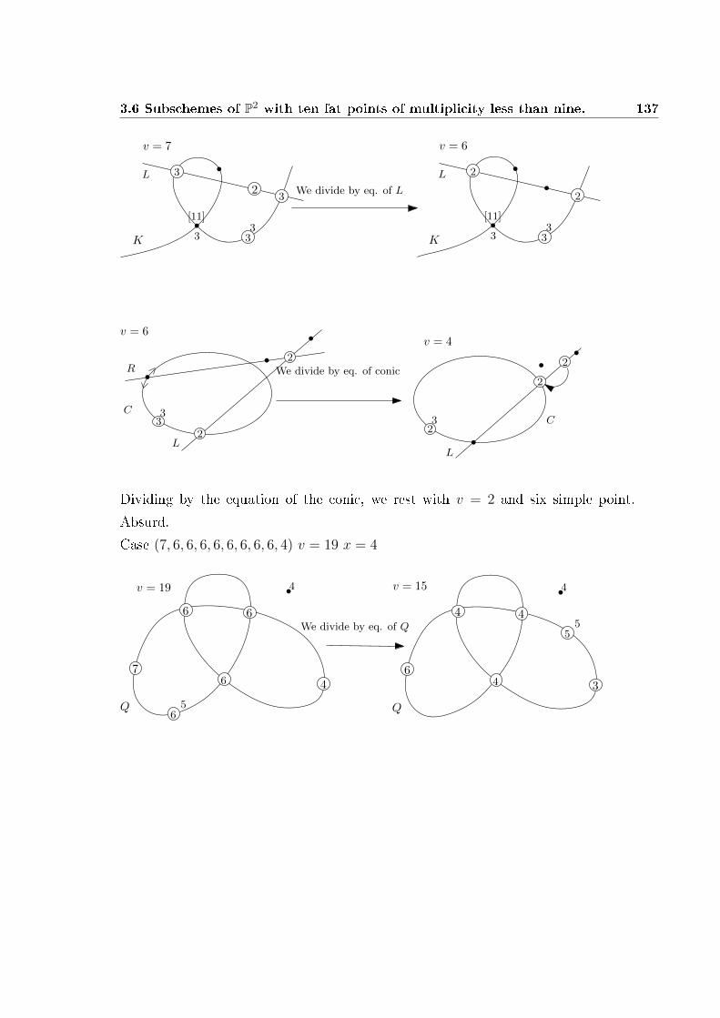
3.6 Subschemes of P2 with ten fat points of multiplicity less than nine. 137
v = 7
3K 3
[11]3
23
3L
We divide by eq. of L
v = 6
3K 3
[11]3
2
2L
2
233
v = 6
C
L
R2
23
v = 4
C
2
L
We divide by eq. of conic
Dividing by the equation of the conic, we rest with v = 2 and six simple point.
Absurd.
Case (7, 6, 6, 6, 6, 6, 6, 6, 6, 4) v = 19 x = 4
Q
6 4
6 6
7
4
We divide by eq. of Q
v = 15
5
Q
4 3
4 4
5
6
4
56
v = 19
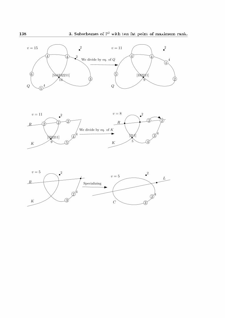
138 3. Subschemes of P2 with ten fat point of maximum rank.
v = 15
Q
3
4 4
6
2
14
[544332211]
2We divide by eq. of Q
45
v = 11
4
Q
2
4 4
4
5
2
9
[332211]
v = 11
5K
2
4
2 2
4
2R
9
[332211]
We divide by eq. of K
v = 8
4K
2
34
2
5
[211]
2R
v = 5
3K
2
24
R Specializing
Lv = 5
3
24
2
C
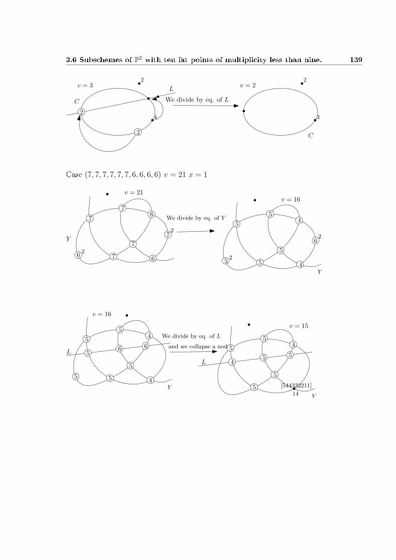
3.6 Subschemes of P2 with ten fat points of multiplicity less than nine. 139
Lv = 3
2
4
2
C
2
We divide by eq. of L
v = 2
3
2
C
Case (7, 7, 7, 7, 7, 7, 6, 6, 6, 6) v = 21 x = 1
7
76
7
67
7
62
2
Y
We divide by eq. of Y
v = 21
6
54
452
2
Y
5
5
5
v = 16
v = 16
54
45
Y
5
5
5
6 65L
We divide by eq. of L
and we collapse a node
54
Y
5
5
5
L5 5
4
14
[544332211]
v = 15

140 3. Subschemes of P2 with ten fat point of maximum rank.
32
Y
3
3
3
4 43
9
[332211]
We divide by eq. of L
v = 10
L
32
Y
3
3
3
3 32
9
[332211]
v = 9
L
v = 9
Q
3 3
9[332211]
3
3
2
2
22
L
R We divide by eq. of Q
v = 5
Q
3 3
9[332211]
2
2
RL
K
v = 5
5
[211]
22
2 2
T
R
L
We divide by eq. of K
K
v = 2
R
Case (7, 7, 7, 7, 7, 7, 7, 6, 6, 5) v = 21 x = 0
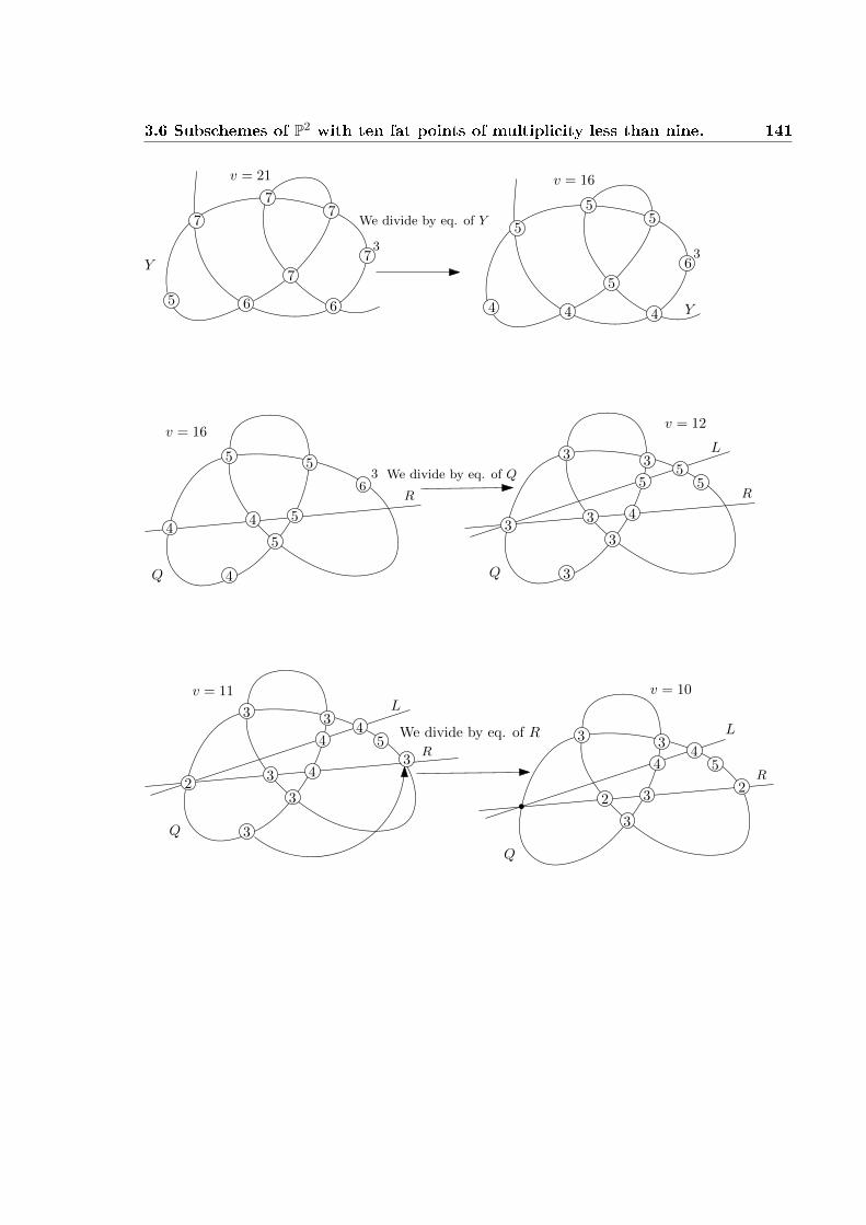
3.6 Subschemes of P2 with ten fat points of multiplicity less than nine. 141
7
77
7
7
5
3
Y
6 6
v = 21
We divide by eq. of Y
6
55
5
5
4
3
4 4
v = 16
Y
5
63
Q
5 5
4
44 5
R
We divide by eq. of Q
v = 16
3
5
Q
3 3
3
3 4
R
3
55
L
v = 12
v = 11
3
5
Q
3 3
3
3 4
R
2
44
L
3
We divide by eq. of R
3
5
Q
3 3
2 3
R
44
L
v = 10
2

142 3. Subschemes of P2 with ten fat point of maximum rank.
v = 10
5K
3
4
3
33
2 2
4L
R T
We divide by eq. of K
v = 7
K
3
2
22
2
T
X
4
3R
v = 6
K
3
2
22
2
T
3
2Specializing
22 T
2
v = 6
3
23
2 R
v = 4
C 2
2
T
2
2
We divide by eq. of C
C
2
v = 2
Case (6, 6, 6, 6, 6, 6, 6, 6, 4, 4) v = 18 x = 2
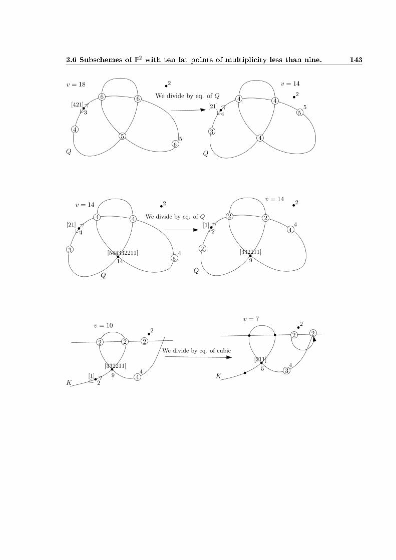
3.6 Subschemes of P2 with ten fat points of multiplicity less than nine. 143
v = 18
6
54
2
6
Q
3
[421]
65
4
3
55
4
Q
4
[21]
4
v = 14
We divide by eq. of Q 2
4
3
2
4
4
[21]
14
[544332211]54
We divide by eq. of Q 2
2
2
44
2
Q
2[1]
9
[332211]
v = 14v = 14
Q
v = 10
K
2
2 2 2
44
9
[332211]
2[1]
We divide by eq. of cubic
v = 7
K
2
2
34
5
[211]
2

144 3. Subschemes of P2 with ten fat point of maximum rank.
v = 4
K
2
24
Specializing
CR
24
2
Dividing by the equation of the conic, we rest with v = 2 and six simple point.
Absurd.
Case (5, 5, 5, 5, 5, 5, 5, 4, 4, 4) v = 15 x = 1
Q
4 4
5 5
2
v = 15
55
5
2 3
3 3
4
2
Q
v = 11
We divide by eq. of Q
Q
2 3
3 3
2444R
42
We divide by eq. of R
v = 11
2
2 3
3 3
4
2333R
Q
v = 10
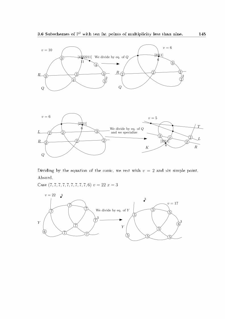
3.6 Subschemes of P2 with ten fat points of multiplicity less than nine. 145
v = 10
Q
2 3
3
4
2333R
11
[4332211] We divide by eq. of Q
2
3
2222
6
[2211]
Q
v = 6
R
v = 6
Q
222R
6
[2211]
322LWe divide by eq. of Qand we specialize
v = 5
K
22
22
6
L
T
R
[2211]
Dividing by the equation of the conic, we rest with v = 2 and six simple point.
Absurd.
Case (7, 7, 7, 7, 7, 7, 7, 7, 7, 6) v = 22 x = 3
7
v = 22
77
7
77
7
6
3
Y
3
We divide by eq. of Y
6
v = 17
5
3
Y
3
55
5
555
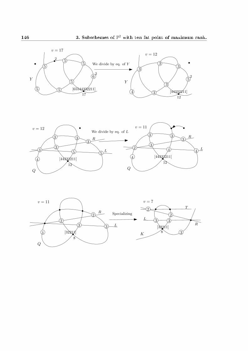
146 3. Subschemes of P2 with ten fat point of maximum rank.
6
v = 17
5
2
Y
55
5
55
2
17
[65544332211]
We divide by eq. of Y
5
v = 12
3
2
Y
33
3
34
12
[44332211]
v = 12
Q
33
12
[44332211]
33
3
4
5 5
R
L
We divide by eq. of Lv = 11
Q
33
12
[44332211]
23
3
4
4 4
R
L
v = 11
Q
8
[32211]
2
3
3 3
R
L2
Specializing
v = 7
K
[32211]
8 3
3
2
2
3
T
R
L

3.6 Subschemes of P2 with ten fat points of multiplicity less than nine. 147
v = 4
K
[11]
3 2
2
2
2Specializing
R
v = 4 223
C
Dividing by the equation of the conic, we can go back to the last passage of case
(5, 5, 5, 5, 5, 5, 5, 5, 5, 5).
By this proves we can improve the proposition 3.6.1 with the follow:
Proposition 3.6.2 Let Z = (b1P1 + ...+ bnPn) be a subscheme of P2, with n ≤ 10
and bi ≤ 8 for all i = 1, ..., n, the respective linear system LZ(v) is non-special,
where v is the critical value of Z.
In the end we have to prove that even h0(IZ(v − 1)) = 0. We use again the
Horace's method. As above we will deal with case by case. By denition of
v, we immediately note that we don't need to add simple points to Z, because
deg(Z) > h0(OP2(v − 1)). To reduce the number of case we apply the Cremona
transformations, and then the Horace's method. We indicate with a = v − 1 and
with r := deg(Z)−h0(OP2(v−1)), r represent the rest of conditions, i.e. the remain
conditions when a = 0.
After the Cremona transformations we get the following cases:
Z1 = (2, 2, 2, 2) a = 2 r = 6
Z2 = (2, 2, 2, 2, 1, 1, 1) a = 3 r = 5
Z3 = (2, 1, 1, 1, 1, 1, 1) a = 2 r = 3
Z4 = (2, 2, 2, 1, 1, 1, 1, 1) a = 3 r = 4
Z5 = (4, 4, 4, 4, 4, 4, 4, 4, 2, 2) a = 12 r = 1
Z6 = (3, 3, 3, 3, 3, 3, 3, 3, 3, 2) a = 9 r = 2
Z7 = (4, 4, 4, 4, 4, 4, 4, 4, 4, 3) a = 12 r = 5
Z8 = (4, 4, 4, 4, 4, 4, 4, 4, 4, 2) a = 12 r = 2
Z9 = (6, 5, 5, 5, 5, 5, 5, 5, 5, 5) a = 16 r = 3
Z10 = (7, 6, 6, 6, 6, 6, 6, 6, 6, 5) a = 19 r = 1

148 3. Subschemes of P2 with ten fat point of maximum rank.
Z11 = (1, 1, 1, 1) a = 1 r = 1
Z12 = (2, 1, 1, 1, 1, 1) a = 2 r = 2
Z13 = (3, 3, 2, 2, 2, 2, 1, 1, 1) a = 5 r = 6
Z14 = (5, 5, 5, 5, 5, 5, 5, 5, 4, 4) a = 15 r = 4
Z15 = (6, 6, 6, 6, 6, 6, 6, 5, 5, 5) a = 18 r = 2
Z16 = (2, 2, 1, 1, 1, 1) a = 2 r = 4
Z17 = (6, 6, 6, 6, 6, 6, 6, 6, 5, 4) a = 18 r = 3
Z18 = (8, 7, 7, 7, 7, 7, 7, 7, 7, 6) a = 22 r = 5
Z19 = (2, 2, 2, 2, 1, 1) a = 3 r = 4
Z20 = (5, 5, 5, 5, 5, 5, 5, 5, 5, 2) a = 15 r = 2
Z21 = (2, 2, 2, 1, 1, 1, 1) a = 3 r = 4
Z22 = (2, 2, 2, 2, 2, 1, 1) a = 3 r = 7
Z23 = (7, 7, 7, 7, 7, 7, 7, 6, 6, 6) a = 21 r = 6
Z24 = (7, 7, 7, 7, 7, 7, 7, 7, 6, 4) a = 21 r = 2
Z25 = (2, 2, 1, 1, 1, 1, 1) a = 2 r = 6
Z26 = (7, 7, 7, 7, 7, 7, 7, 7, 7, 7) a = 22 r = 4
Z27 = (2, 2, 2, 1, 1) a = 2 r = 5
Z28 = (2, 2, 2, 2, 1, 1, 1, 1) a = 3 r = 6
Z29 = (3, 2, 2, 2, 2, 1, 1, 1) a = 4 r = 6
Z30 = (2, 2, 1, 1, 1) a = 2 r = 3
Z31 = (3, 2, 2, 2, 1, 1, 1) a = 3 r = 8
Z32 = (8, 8, 8, 8, 8, 8, 8, 7, 7, 6) a = 24 r = 4
Z33 = (8, 8, 8, 8, 8, 8, 7, 7, 7, 7) a = 24 r = 3
Z34 = (8, 8, 8, 8, 8, 8, 8, 8, 6, 6) a = 24 r = 5
Z35 = (8, 8, 8, 8, 8, 8, 8, 8, 6, 4) a = 24 r = 1
Z36 = (8, 8, 8, 8, 8, 8, 8, 8, 8, 7) a = 25 r = 1
We note that these cases are more easier and less than precedent cases.
Remark 3.6.3 Let Z ⊂ X be subschemes of P2; it easy to show that if h0(LZ(d)) =
0 then h0(LX(d)) = 0 too.
By this remark we can reduce the listed above cases because : Z19 is contained in

3.6 Subschemes of P2 with ten fat points of multiplicity less than nine. 149
Z2, Z28, Z25 and Z31; Z21 is contained in Z4 and Z5 is contained in Z7. The cases
with a = 2, 3 are easy to show, and we don't give the proof here.
Case Z5 = (4, 4, 4, 4, 4, 4, 4, 4, 3, 3) a = 12 r = 1
a = 12
K
4
4
6 We divide by eq. of cubic
3
2
[1,3]
4
a = 9
K
3
2
4
3
3
[1]
43 3R
a = 8
K
3
2
4
2
3
[1]
32 2
We divide by eq. of K
R
a = 5
K
24
3 R
a = 5
K
R
3
3
2
2L
We divide by eq. of L
a = 4
K32
L
2 R
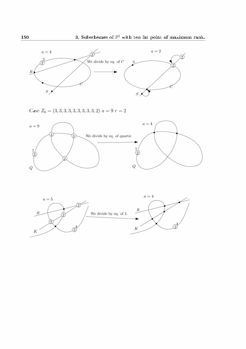
150 3. Subschemes of P2 with ten fat point of maximum rank.
32
2
C
S
a = 4
32
C
a = 2
2
S
We divide by eq. of C
R
Case Z6 = (3, 3, 3, 3, 3, 3, 3, 3, 3, 2) a = 9 r = 2
a = 9
Q
3 3
237
We divide by eq. of quartic
a = 4
Q
27
a = 5
K 24
a = 4
K 24
We divide by eq. of LRR
2
2
2

3.6 Subschemes of P2 with ten fat points of multiplicity less than nine. 151
a = 1
K4
R
Case Z8 = (4, 4, 4, 4, 4, 4, 4, 4, 4, 2) a = 12 r = 2
We divide by eq. of cubic
49
a = 12
2
K
39
a = 9
2
K

152 3. Subschemes of P2 with ten fat point of maximum rank.
29
a = 6
2 We divide by eq. of K
K
7
a = 3
K
2
R
2
a = 2
K
C
Case Z9 = (6, 5, 5, 5, 5, 5, 5, 5, 5, 5) a = 16 r = 3
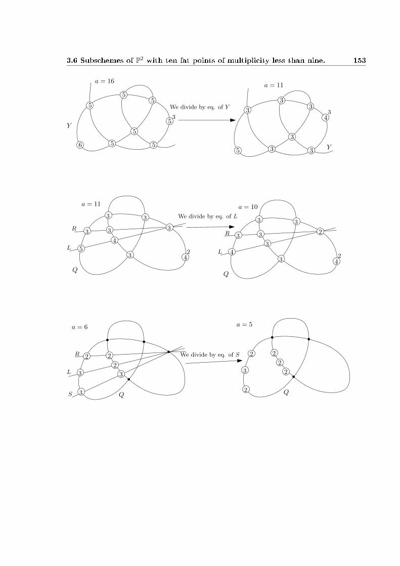
3.6 Subschemes of P2 with ten fat points of multiplicity less than nine. 153
53
Y
55
5
55
5
6
a = 16
We divide by eq. of Y3
5
3
3
3
33
4
Y
3
a = 11
Q
3 42
33
5
3 3 3
4
R
L
a = 11
We divide by eq. of L
Q
3 42
33
3 3 2
4
3
a = 10
L
R
a = 6
22
3
2
Q
3
3
We divide by eq. of SR
L
S
a = 5
22
3
2
Q
2
2
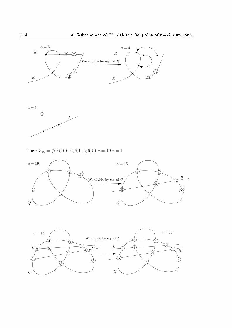
154 3. Subschemes of P2 with ten fat point of maximum rank.
a = 5
2K
2
33
R2
We divide by eq. of R
a = 4
2K
33
R
a = 1
2L
Case Z10 = (7, 6, 6, 6, 6, 6, 6, 6, 6, 5) a = 19 r = 1
a = 19
Q
7
66
5
66
We divide by eq. of Q
a = 15
Q
44
3546
55
R
Q
44
355
445 5
5
We divide by eq. of L
L R
Q
44
355
444 4
4L
a = 13
R
a = 14

3.6 Subschemes of P2 with ten fat points of multiplicity less than nine. 155
a = 13
Q
4
5
44
R4 4
4L
3
14[544332211]
We divide by eq. of Q
Q
2
4
33
R3 3
3L
9[332211]
a = 9
a = 8
Q
2
3
22
R3 3
3L
9[332211]
We divide by eq. of L
Q
2
3
22
L
9[332211]
222
a = 7
R
a = 7
K 9
[332211]
R
2
2 2L
2 2 2
3Sa = 4
K 5
[211]
R L
3We divide by eq. of K

156 3. Subschemes of P2 with ten fat point of maximum rank.
a = 3
K 5
[211]
L
22
We divide by eq. of cubic
a = 0
Case Z13 = (3, 3, 2, 2, 2, 2, 1, 1, 1) a = 5 r = 6
24
3
a = 53
2
4
2
a = 23
2
KK
We divide by eq. of cubic
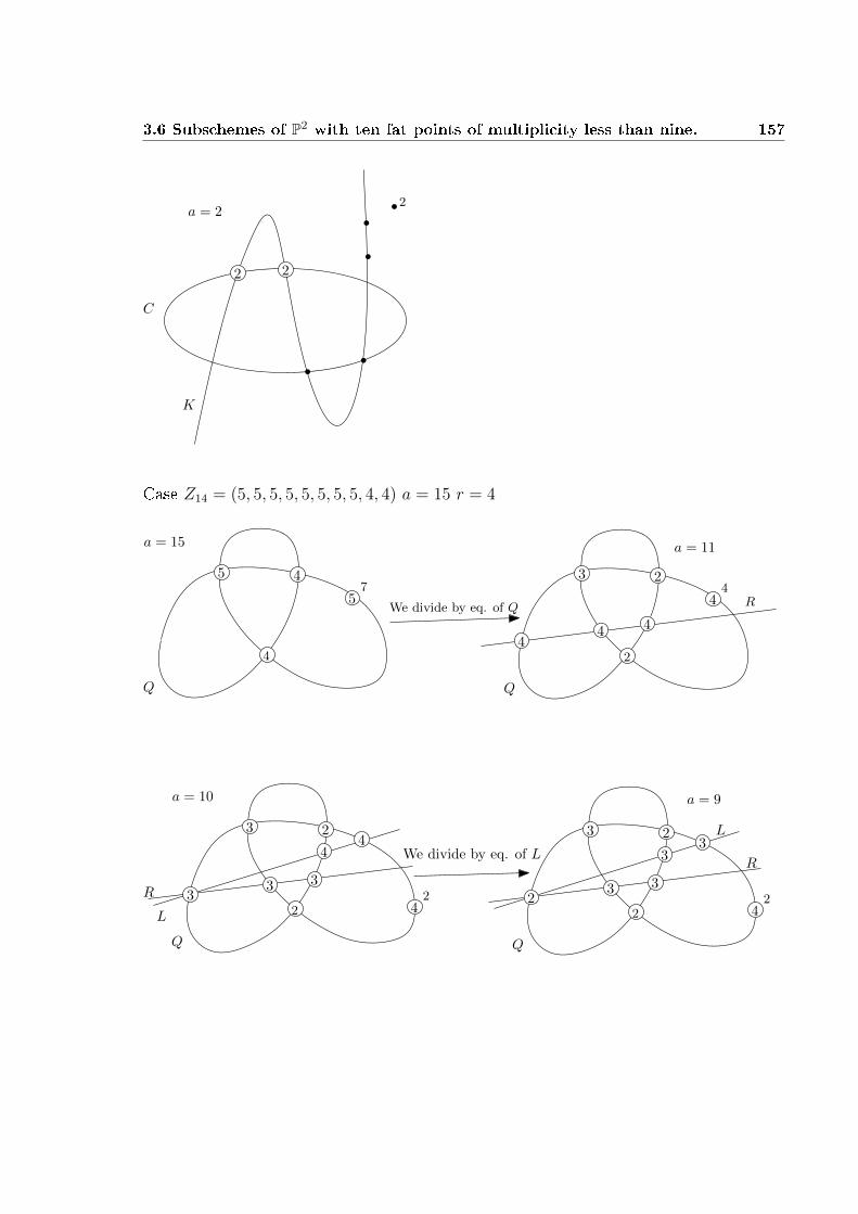
3.6 Subschemes of P2 with ten fat points of multiplicity less than nine. 157
a = 22
K
C
22
Case Z14 = (5, 5, 5, 5, 5, 5, 5, 5, 4, 4) a = 15 r = 4
a = 15
7
Q
4
5 4
5We divide by eq. of Q
4
Q
2
3 2
4
444
a = 11
R
a = 10
Q
2
3 2
3 33
44
24
We divide by eq. of L
R
L
Q
2
3 2
3 32
33
24
a = 9
L
R
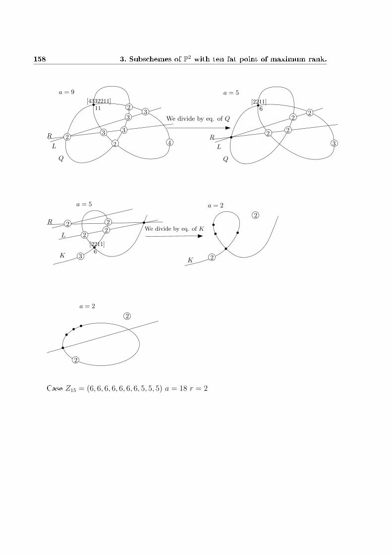
158 3. Subschemes of P2 with ten fat point of maximum rank.
a = 9
Q
2
2
3 32
33
4
11[4332211]
R
L
We divide by eq. of Q
a = 5
2
3
6[2211]
2
22
L
R
Q
a = 5
K
R
L
3
22
2
6
[2211]
We divide by eq. of K2
a = 2
K 2
2
a = 2
2
2
Case Z15 = (6, 6, 6, 6, 6, 6, 6, 5, 5, 5) a = 18 r = 2
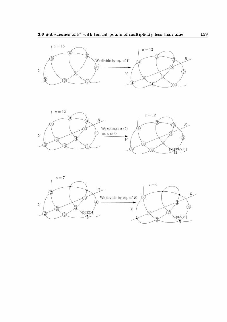
3.6 Subschemes of P2 with ten fat points of multiplicity less than nine. 159
6
6
6
5
3
Y
6 6
55
We divide by eq. of Y
5
4
Y
33
4
4 4
R
5
5
4
a = 13a = 18
5
4
Y
33
4
4 4
R
4
4
3
We collapse a (5)
on a node
a = 12
5
4
Y
33
4
4
R
4
4
314
[544332211]
a = 12
4Y
R
3
3
29
[332211]2
2
2
We divide by eq. of R
a = 7
4Y
R
2
2
9
[332211]2
2
2
a = 6
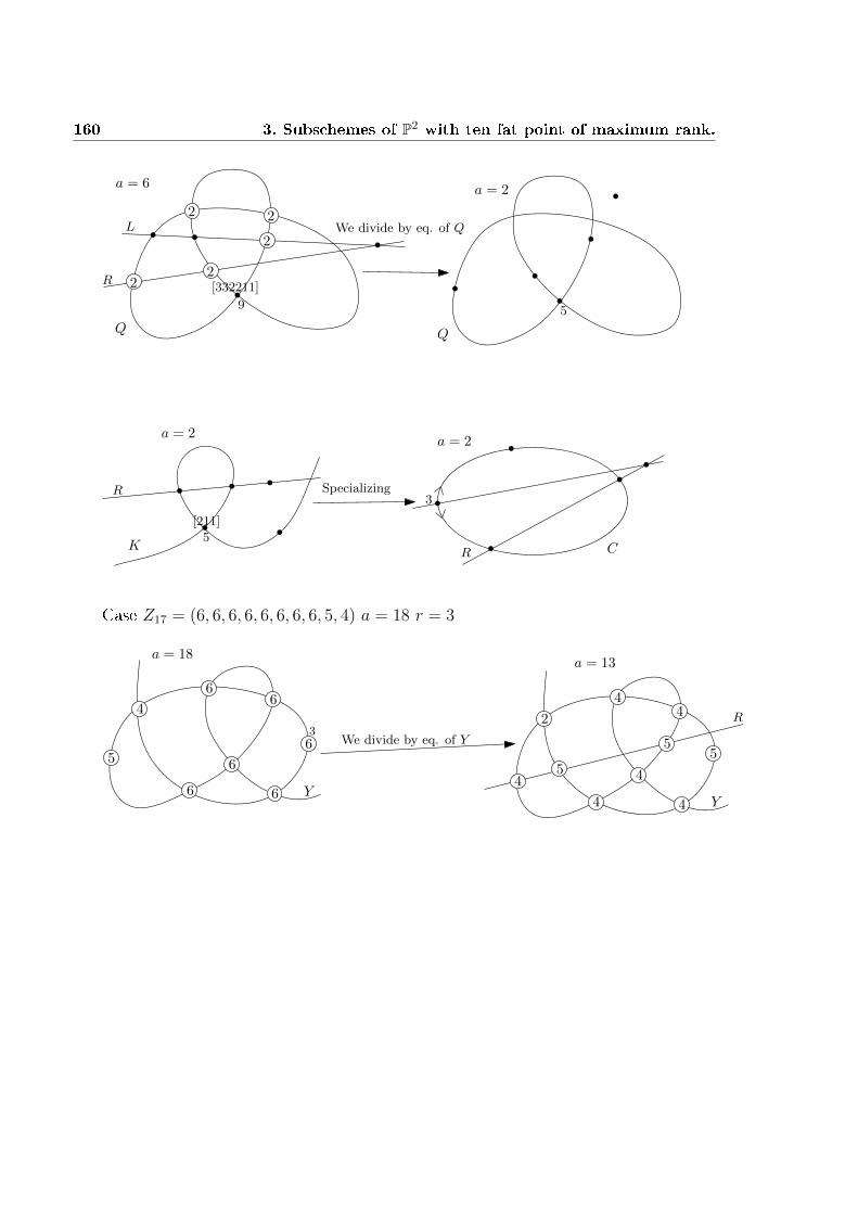
160 3. Subschemes of P2 with ten fat point of maximum rank.
a = 6
Q
9
[332211]
2 2
2
22
L
R
We divide by eq. of Q
Q
5
a = 2
a = 2
K5
[211]
R Specializing
C
3
a = 2
R
Case Z17 = (6, 6, 6, 6, 6, 6, 6, 6, 5, 4) a = 18 r = 3
63
64
Y
5
6
6
66
a = 18
Y
a = 13
We divide by eq. of Y5
2
4
4
4
44
45
5
R
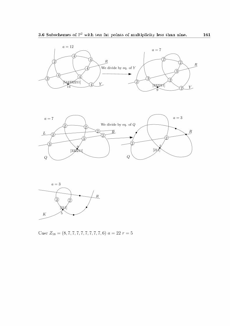
3.6 Subschemes of P2 with ten fat points of multiplicity less than nine. 161
Y
a = 12
2
4
4
44
34
4
R
14
[544332211]
Y
a = 7
2
23
R
9
[332211]
2
2
2
3We divide by eq. of Y
a = 7
Q
3
2R
2L
9[332211]
3
2
2 2We divide by eq. of Q
Q
25
[211]
2
R
a = 3
a = 3
5
[211]
K
2 2R
Case Z18 = (8, 7, 7, 7, 7, 7, 7, 7, 7, 6) a = 22 r = 5
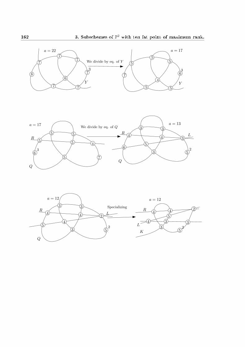
162 3. Subschemes of P2 with ten fat point of maximum rank.
7
a = 22
77
77
7
8
We divide by eq. of Y
Y6
367
a = 17
5
4
5
55
5
Y
3
a = 17
Q
65
55
45 5
7
3
R
a = 13
Q
3
33
4 4 3
R L
652
5
We divide by eq. of Q
a = 12
Q
3
33
4 4 2
RL
552
4
Specializing
a = 12
K
R 24 4
4L
5
3 33
52
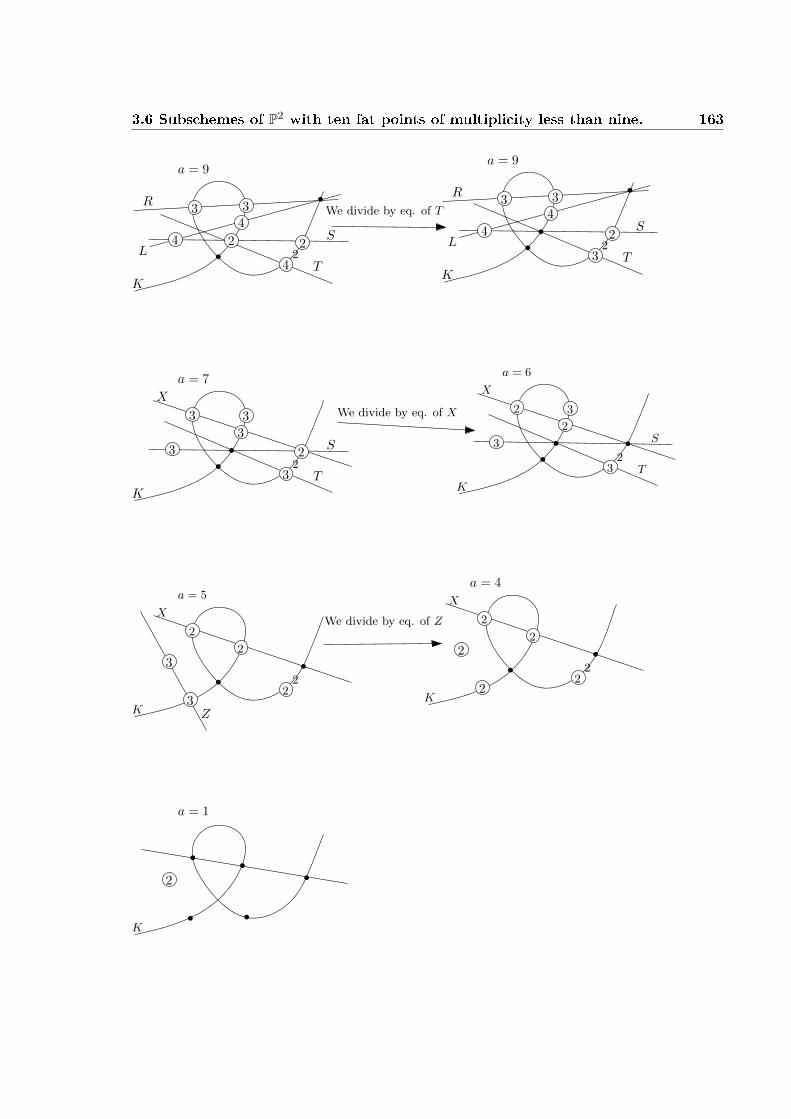
3.6 Subschemes of P2 with ten fat points of multiplicity less than nine. 163
a = 9
R
4L
4
2
K
S
3 3
T2
4
We divide by eq. of T
2
a = 9
R
4L
4
2
K
S
3 3
T2
3
a = 7
K
S
3
T2
3
3
3
3
2
X
a = 6
K
S
3
T2
3
3
2
2
X
We divide by eq. of X
a = 5
K
22
2
2
XWe divide by eq. of Z
3
3Z
a = 4
K
22
2
2
X
2
2
a = 1
K
2
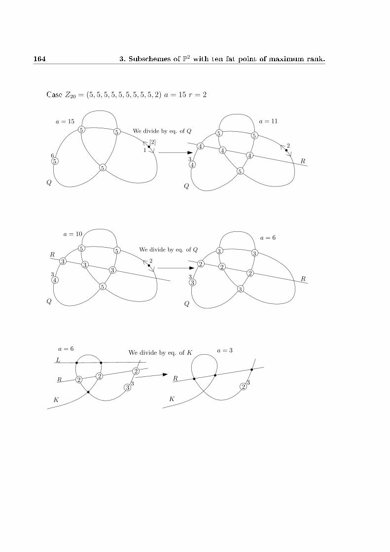
164 3. Subschemes of P2 with ten fat point of maximum rank.
Case Z20 = (5, 5, 5, 5, 5, 5, 5, 5, 5, 2) a = 15 r = 2
a = 15
Q
5 5
556
1
[2]
We divide by eq. of Q
Q
5 5
543
2
R
44
4
a = 11
Q
5 5
543
233
3
R
a = 10
We divide by eq. of Q
Q
3 3
333 R
2 22
a = 6
a = 6
K
32
22
R
L
3
We divide by eq. of K a = 3
K
2
R3
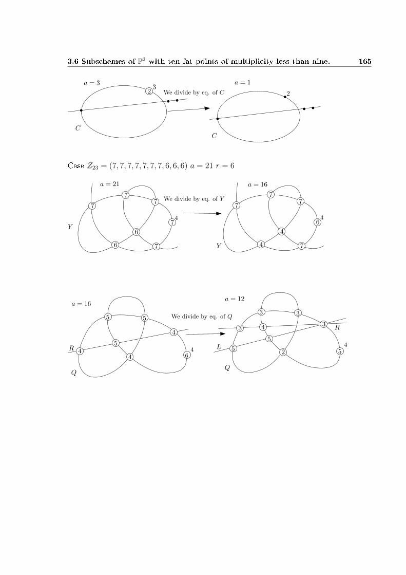
3.6 Subschemes of P2 with ten fat points of multiplicity less than nine. 165
23
C
a = 3
We divide by eq. of C
C
2
a = 1
Case Z23 = (7, 7, 7, 7, 7, 7, 7, 6, 6, 6) a = 21 r = 6
7
a = 21
77
6
7
4
Y
6 7
6
a = 16
4
4
4 7Y
We divide by eq. of Y7
77
a = 16
Q
64
4
5 5
4
We divide by eq. of Q
5
4
R
a = 12
Q
4
3 3
52
R3 4 3
5
5L

166 3. Subschemes of P2 with ten fat point of maximum rank.
a = 11
Q
2
3 3
52
R 3 4
4
4
2
L
Specializing a = 11
5K3 2
4
4 42
2
3
3 SR
L
a = 8
K
4
3 3
2
2R
L
S
42
T
We divide by eq. of T
a = 7
K
4
3 3
R
L
22
32
X
a = 6
K
4
3 3L
222
XR
We divide by eq. of Ra = 5
K
3
22
X3
3
Z
a = 4
K
3
22
2
2We divide by eq. of K
X
a = 1
K
2
2

3.6 Subschemes of P2 with ten fat points of multiplicity less than nine. 167
Case Z24 = (7, 7, 7, 7, 7, 7, 7, 7, 6, 4) a = 21 r = 2
Q
76
5
7
77We divide by eq. of Q
2
[134]
a = 17
Q
5
5
55
4
[13]
6
5
a = 21
a = 12
Q
2
3
3
[1]3
3
5
4 4 R
13
[54332211]
a = 13
Q
3
3
3
[1]3
4
5
5 5 R
3
We divide by eq. of R
a = 8
Q
3
8
[32211]
R 23
4 4
L
We divide by eq. of L
a = 7
Q
3
8
[32211]
R23
3 3
L
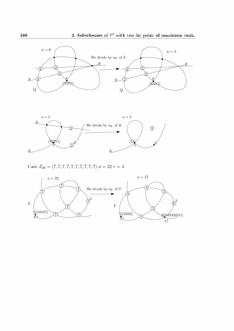
168 3. Subschemes of P2 with ten fat point of maximum rank.
a = 6
Q
2
8
[32211]
R2
S 3
3
We divide by eq. of S
a = 5
Q
2
8
[32211]
R2
S 2
2
a = 5
K
X
2
23
8[32211]
We divide by eq. of K
a = 2
K
2
3[11] 3
Case Z26 = (7, 7, 7, 7, 7, 7, 7, 7, 7, 7) a = 22 r = 4
7
77
7
7
3
Y
7 76
[123457]
a = 22
6
5
3
Y
7
[12345]
55
5
5
17
[65544332211]
a = 17
We divide by eq. of Y
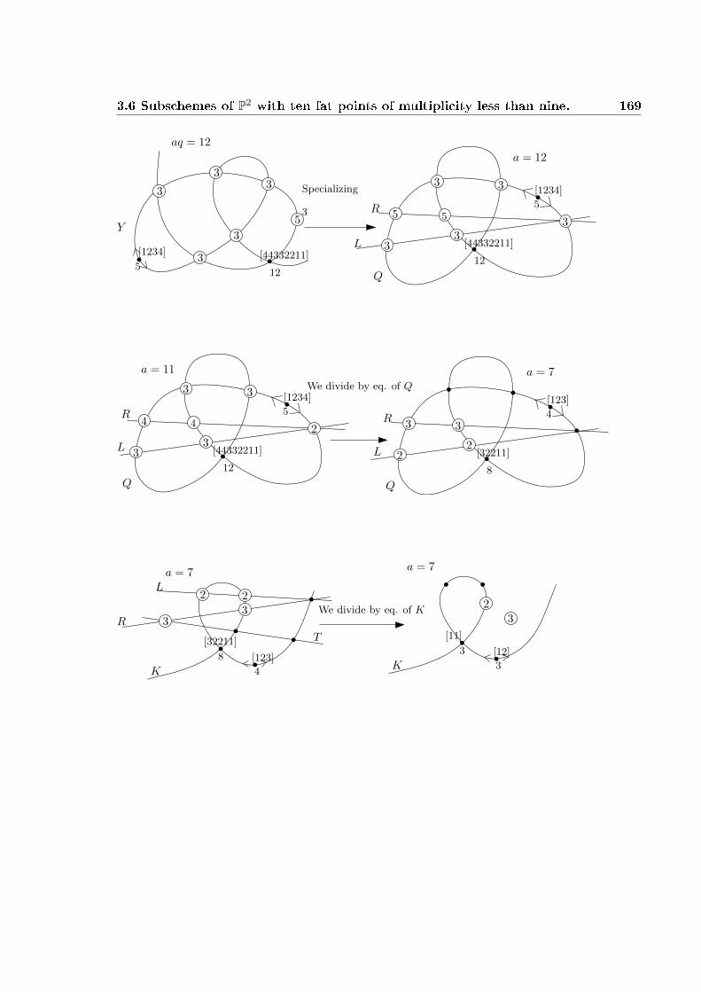
3.6 Subschemes of P2 with ten fat points of multiplicity less than nine. 169
5
3
3
Y
5
[1234]
33
3
312
[44332211]
aq = 12
Specializing
Q
3
5
[1234]3
5 5R
L 33
3
12
[44332211]
a = 12
Q
3
5
[1234]3
4 4
33
2
12
[44332211]
We divide by eq. of Q
Q
4
[123]
R
2
33
28
[32211]
a = 7
LL
R
a = 11
a = 7
K
8
[32211]
R3
4
[123]
We divide by eq. of K3
L
T
2 2
a = 7
K
3
[11]
3
[12]
2
3
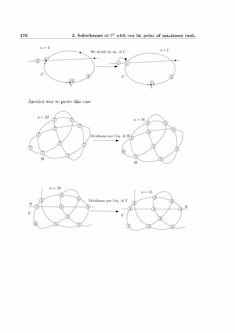
170 3. Subschemes of P2 with ten fat point of maximum rank.
a = 4
3
[12]
2
C
2
3
We divide by eq. of C
2
[1]
C
2
2
2
a = 2
Another way to prove this case
W
7 7
7
7
7
7
7
7
7
7
Dividiamo per l’eq. di W
a = 22
W
5
6
5 5
5
5
5
5
5
5
a = 16
Y
5 5 5
5
55
5
5
56
Dividiamo per l’eq. di Y
a = 16
Y
4
35 3
3
33
3
4 4
a = 11
RR

3.6 Subschemes of P2 with ten fat points of multiplicity less than nine. 171
a = 10
Y
3
35 3
3
33
3
3 3
Specializziamo
a = 10
Q
3 3
5
33
3
3
333
R
LR
a = 6
Q
R
4
2L
22 2
22
Specializziamo
a = 6
22
K4
2
T
22 2 R
S
L
a = 5
22
K3
22 2 R
S
L
Dividiamo per l’eq. di Ra = 4
22
K3
R
L

172 3. Subschemes of P2 with ten fat point of maximum rank.
a = 5
22
K3
22 2 R
S
L
Dividiamo per l’eq. di Ra = 4
22
K3
R
L
Case Z29 = (3, 2, 2, 2, 2, 1, 1, 1) a = 4 r = 6
24
a = 4
K
3
We divide by eq. of cubic
4
a = 1
K
2
R
2
Case Z32 = (8, 8, 8, 8, 8, 8, 8, 7, 7, 6) a = 24 r = 4
83
a = 24
76
8
Y
8
88
7
We divide by eq. of Y 54
6
Y
6
66
7
a = 19
R
67
7
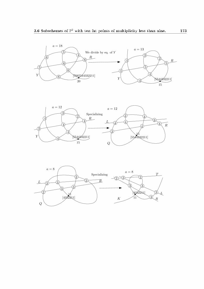
3.6 Subschemes of P2 with ten fat points of multiplicity less than nine. 173
54
6
Y
6
6
a = 18
R
56
6
20
[7665544332211]
We divide by eq. of Y3
2
Y
a = 13
R
45
5
15
[5544332211]4
4
4
32
Y
a = 12
R
34
4
15
[5544332211]4
4
4
Specializing
a = 12
Q
4
3
444 4
3L
2
15[5544332211]
R
a = 8
Q
2R
3L
11[4332211]
2
23
3
3
Specializinga = 8
11
[4332211]
K R
L
2 2
3 3
3
3
T2

174 3. Subschemes of P2 with ten fat point of maximum rank.
a = 5
6
[2211]
K R
L
2T
2
2
2
2
We divide by eq. of R2
a = 4
6
[2211]
K R
L
2T
2
2
a = 1
K
L
2
Case Z33 = (8, 8, 8, 8, 8, 8, 7, 7, 7, 7) a = 24 r = 3
83
a = 24
77
7
Y
8
88
7
We divide by eq. of Y
7
55
5
Y
6
66
a = 19
R
7
76
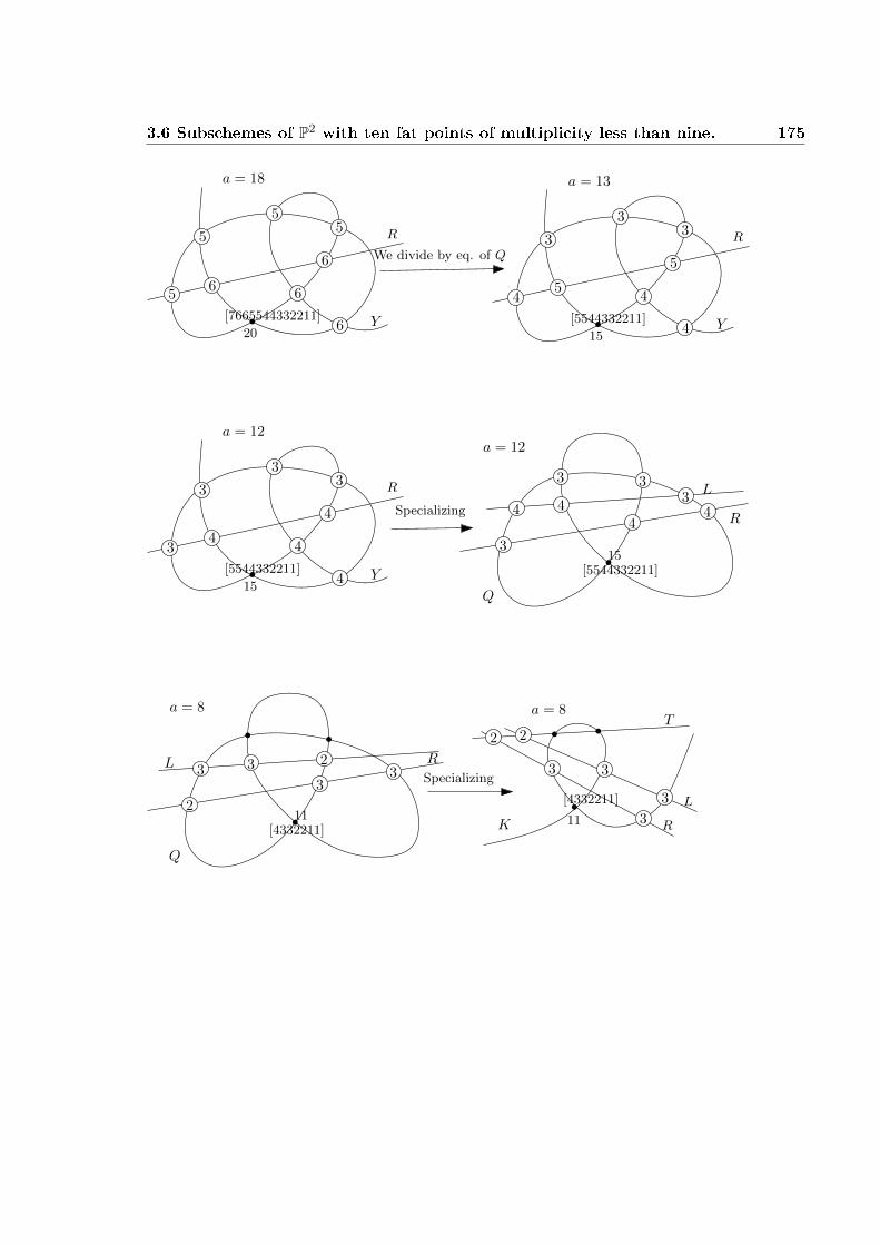
3.6 Subschemes of P2 with ten fat points of multiplicity less than nine. 175
55
5
Y
6
6
a = 18
R
6
6
5
20
[7665544332211]
We divide by eq. of Q
33
3
Y
4
4
a = 13
R
15
[5544332211]
5
5
4
33
3
Y
4
4
a = 12
R
15
[5544332211]
4
4
3
Specializing
a = 12
Q
3
3
44 R
4 43
L3
15[5544332211]
a = 8
Q
2
RL
11[4332211]
3 3
33
2Specializing
a = 8
11
[4332211]
K R
L
2 2
3 3
3
3
T
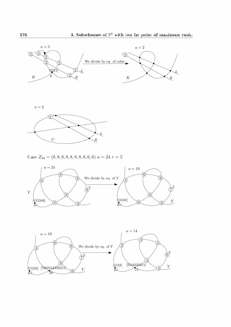
176 3. Subschemes of P2 with ten fat point of maximum rank.
a = 5
6
[2211]
K R
L
2 2
2 2
2
2
a = 2
K R
L
22
We divide by eq. of cubic
a = 2
C R
L
2
Case Z34 = (8, 8, 8, 8, 8, 8, 8, 8, 6, 6) a = 24 r = 5
8
a = 24
6
3
Y
5
[12346]8
8
8
88 We divide by eq. of Y
7
a = 19
4
3
6
[1234]6 6
6
66
Y
7
a = 19
4
2
6
[1234]6
6
66
Y20
[7665544332211]
We divide by eq. of Y
6
a = 14
2
2
4
[123] Y15
[5544332211]
44
4
4
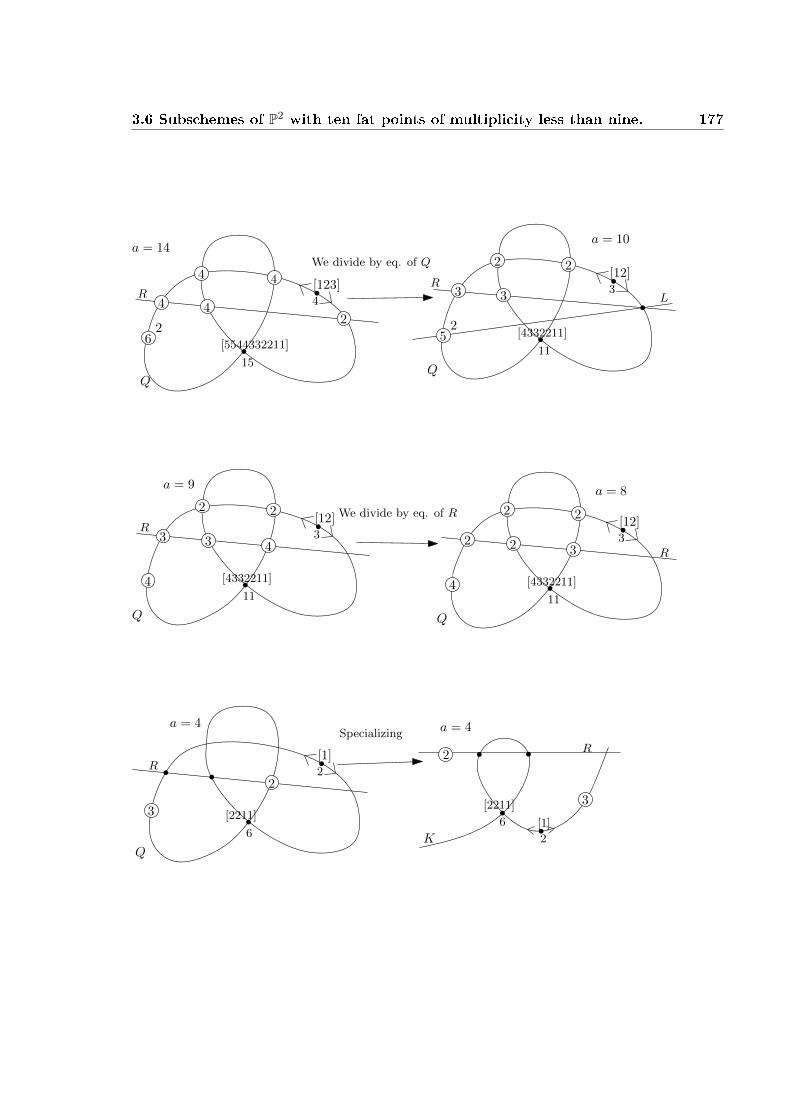
3.6 Subschemes of P2 with ten fat points of multiplicity less than nine. 177
a = 14
Q
62
4
[123]4 4
2
R4 4
15
[5544332211]
We divide by eq. of Q
a = 10
Q
3
[12]R
3 3
11
[4332211]
2 2
52
L
a = 9
Q
3
[12]R
3 3
11
[4332211]
2 2
4
4
We divide by eq. of R
a = 8
Q
3
[12]
2 2
11
[4332211]
2 2
4
3 R
a = 4
Q
2
[1]R
6
[2211]
2
3
Specializinga = 4
K
6
[2211]
2
[1]
R2
3
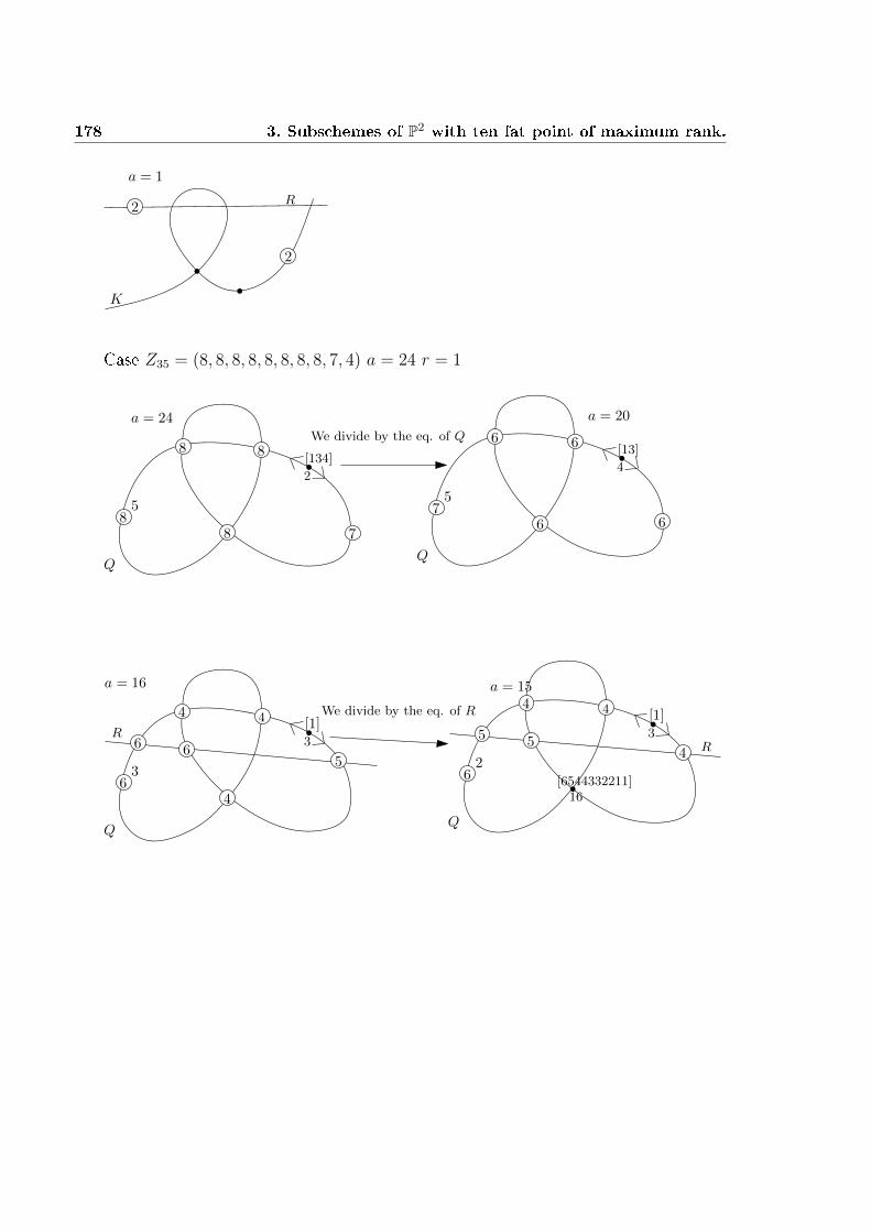
178 3. Subschemes of P2 with ten fat point of maximum rank.
a = 1
K
R2
2
Case Z35 = (8, 8, 8, 8, 8, 8, 8, 8, 7, 4) a = 24 r = 1
a = 24
Q
87
5
8
88
2
[134]
We divide by the eq. of Q
a = 20
Q
75
6
4
[13]6 6
6
a = 16
Q
63
4
3
[1]4 4
6 65
We divide by the eq. of R
R
Q
62
3
[1]4 4
5 54
16[6544332211]
a = 15
R
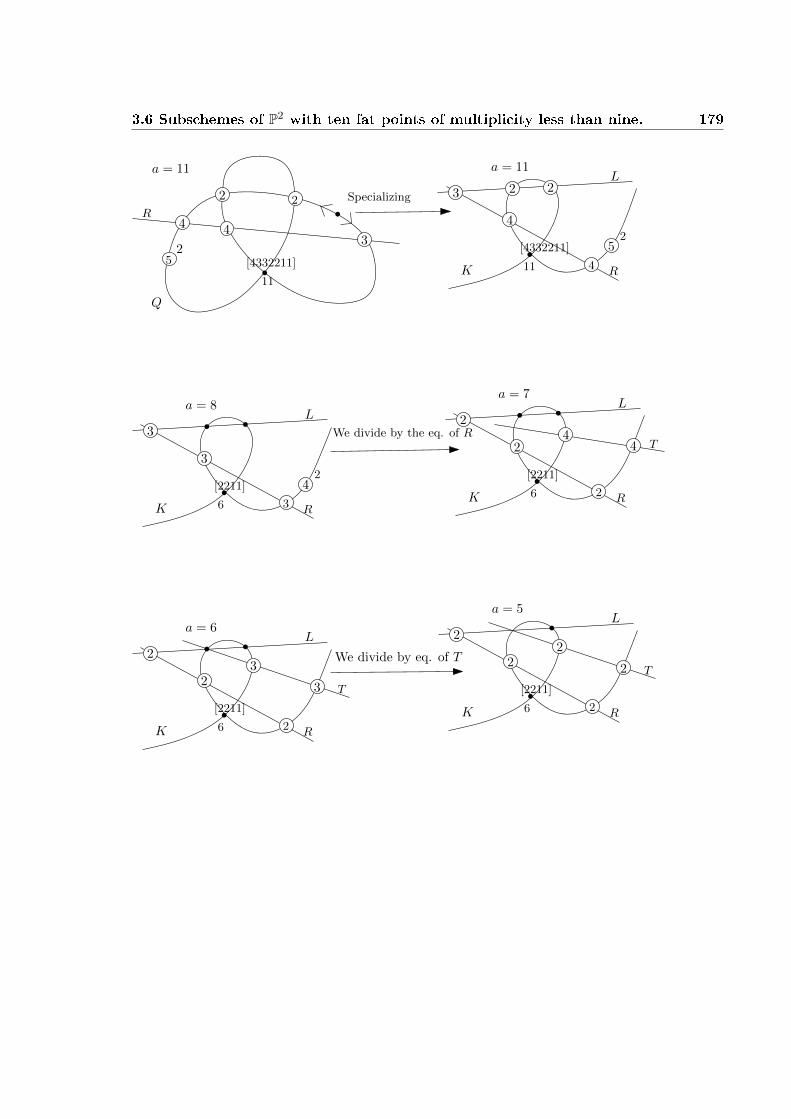
3.6 Subschemes of P2 with ten fat points of multiplicity less than nine. 179
a = 11
Q
52
2 2
4 43
R
11
[4332211]
Specializing
a = 11
11
[4332211]
K R
4
4
5
L23 2
2
a = 8
6
[2211]
K R
3
3
4
L
3
2
We divide by the eq. of R
a = 7
6
[2211]
K R
2
2
L
2
T44
a = 6
6
[2211]
K R
2
2
L
23
3 T
We divide by eq. of T
a = 5
6
[2211]
K R
2
2
L
22
2 T
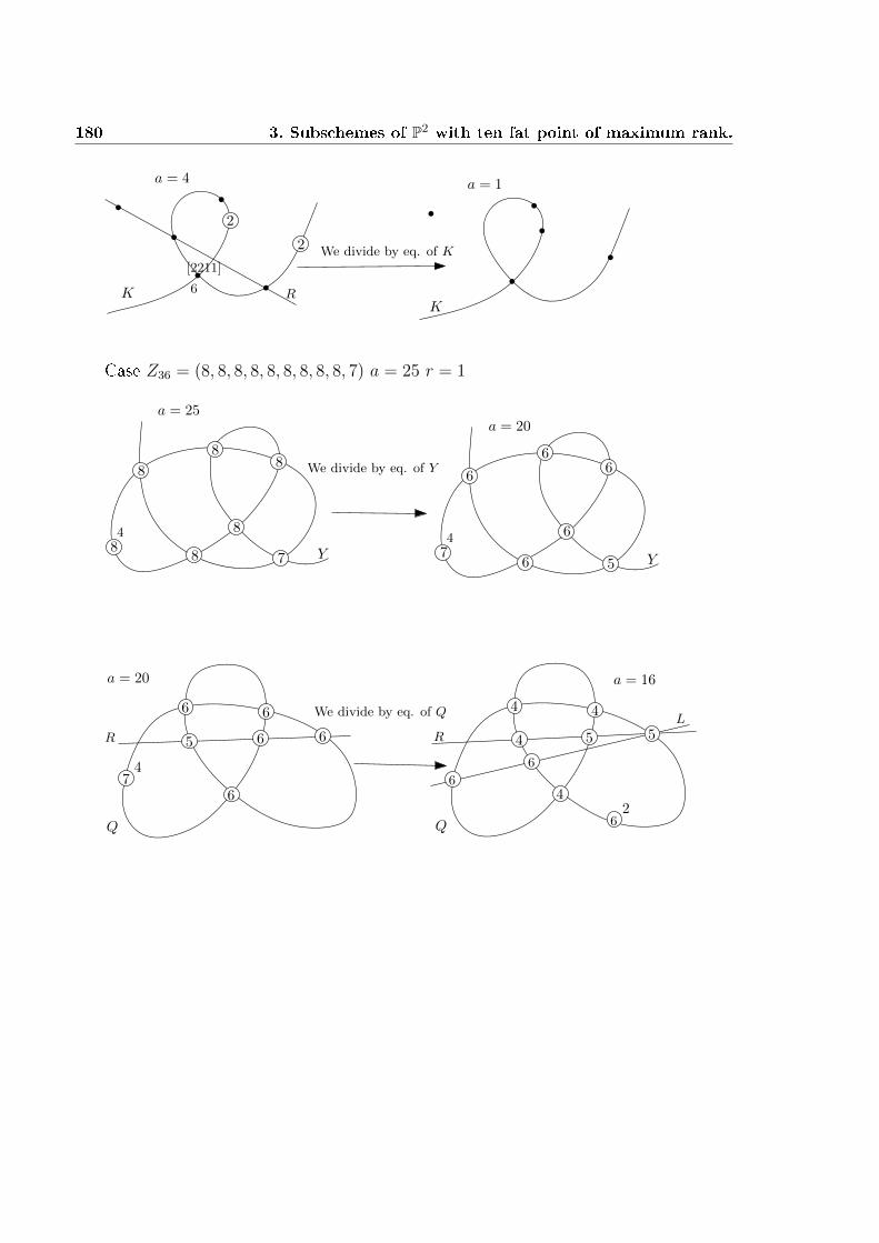
180 3. Subschemes of P2 with ten fat point of maximum rank.
a = 4
6
[2211]
K R
2
2 We divide by eq. of K
a = 1
K
Case Z36 = (8, 8, 8, 8, 8, 8, 8, 8, 8, 7) a = 25 r = 1
88 7
8
88
8
4
Y
a = 25
75
6
4
Y
6
6
6
6
a = 20
We divide by eq. of Y
a = 20
Q
74
6
6 6
R 665
We divide by eq. of Q
Q
4
R 5
4 4
4
62
L5
6
6
a = 16

3.6 Subschemes of P2 with ten fat points of multiplicity less than nine. 181
Q
R 5
4 4
4
6
L
55
4
16
[6544332211]
a = 15We divide by eq. of Q
Q
R 4
2 2
3
5
L
44
3
11
[4332211]
a = 11
a = 11
11
[4332211]
K
24 2
L
R
T
4
433
5
We divide by eq. of K
a = 8
6
[2211]
K
4
L
T
22
4
3
3R
a = 7
6
[2211]
K
3
L
T
2
2
3R
4S
We divide by eq. of S
a = 6
6
[2211]
K
3
L
2
2
2R
3

182 3. Subschemes of P2 with ten fat point of maximum rank.
a = 6
4 2
2
2
C L3
2
3
We divide by eq. of C
R
a = 4
2
C L3
2
R
a = 3
2R
C2
2
a = 1
C2
We divide by eq. of C
For all case that we have just studied the method is true. We conclude summa-
rizing our result in the following theorem
Theorem 3.6.4 Every subscheme of P2 in the form Z = (b1P1 + ... + bnPn) with
n ≤ 10 and 4 ≤ bi ≤ 8 for all i = 1, ..., n, has maximum rank.
Moreover we have just veried that the conjecture 3.2.7 holds for all linear system
with exactly ten assigned point in base locus, with multiplicity minor than 9.
Bibliography
[1] E. Ballico, L. Chiantini, On smooth subcanonical varieties of codimension two
in Pn, n ≥ 4, Annali Mat. Pura Appl. 135, 99-117, (1983)
[2] Beorchia, V-Ellia, Ph.: Normal bundle and complete intersections, Rend. Sem.
Mat. Univ. Politecnico Torino, vol. 48,4, 553-562 (1990)
[3] Ciliberto, C.: Geometric aspects of polynomial interpolation in more variables
and Waring's problem, European Congress of Mathematics, Vol. I (Barcelona,
2000), 289-316.
[4] C. Ciliberto, R. Miranda: Homogeneous interpolation on ten points,
arXiv:0812.0032 (2008).
[5] D'Almeida, J.: Une involution sur un espace de modules de brés instantons,
Bull. Soc. math. France, 128, 577-584 (2000)
[6] Ellia, Ph.: Sur les brés uniformes de rang (n+1) sur Pn. Mémoire de la So-
ciété Mathématique de France, nouvelle série n 7, Tome 110, Fascicule 1, 1-60,
Gauthier-Villars (1982)
[7] Ellia, Ph.: Arithmetically Cohen-Macaulay space curves reloaded, preprint
(2011).
[8] Ellia, Ph.: Double structures and normal bundle, J. London Math. Soc., (2) 58,
18-26 (1998)
[9] Ellia, Ph.: Exemples de courbes de P3 à bré normal semi-stable, stable, Math.
Ann., 264, 389-396 (1983)
183

184 BIBLIOGRAPHY
[10] Ellia, Ph.-Franco, D.-Gruson, L.: On subcanonical surfaces of P4, Math. Z.,
251, 257-265 (2005)
[11] Ellingsrud, G.: Sur le schéma de Hilbert des variétés de codimension 2 dans Pe
Ó cône de Cohen-Macaulay, Ann. scient. Éc. Norm. Sup., 4e série, t. 8, 423-432
(1975)
[12] Fulton, W.: Intersection theory
[13] Gruson, L.-Peskine, Ch.: Genre des courbes de l'espace projectif, 31-60, LNM
687 (1978)
[14] Hartshorne, R.: Stable rank two vector bundles
[15] Hartshorne, R.: On the classication of algebraic space curves, II, in Alge-
braic Geometry-Bowdoin 1985, Proceedings of Symposia in Pure Mathematics,
vol.46, part 1, 145-164, Ed. A.M.S. (1987)
[16] Mori, S.: On the degree and genera of curves on smooth quartic surfaces in P3,
Nagoya Math. J., 96, 127-132 (1984)
[17] Newstead, P.E.: A space curve whose normal bundle is stable, J. London Math.
Soc., 28, 428-434 (1983)
[18] Okonek, C.-Schneider,M-Spindler, H.: Vector Bundles on complex projective
Spaces. Progress in Mathematics, J. Coates and S. Helgason.
[19] Perrin, D.: Courbes passant par m points généraux de P3, Bull. Soc. Math. de
France, Mémoire (nouvelle série), n. 28/29 (1987)
[20] Sierra, J.C.: A degree bound for globally generated vector bundles, Math. Z.,
[21] Sierra, J.C.-Ugaglia, L.: On globally generated vector bundles on projective
spaces
[22] Sukmoon Huh: On triple Veronese embeddings of Pn in the Grassmannians,
arXiv 0806.0777v6 (2010)
BIBLIOGRAPHY 185
[23] Van de Ven, A.: On uniform vector bundles, Math. Ann., 195, 245-248 (1978)
[24] C. Ciliberto, R. Miranda: Homogeneous interpolation on ten points,
arXiv:math.AG/0406591 (2005)