BIT 10 (1970), 217--227

SOME R E L A T I O N S H I P S B E T W E E N I M P L I C I T

R U N G E - K U T T A , C O L L O C A T I O N A N D

LANCZOS v M E T H O D S ,

A N D T H E I R S T A B I L I T Y P R O P E R T I E S

K. W R I G H T

Abstract . In this paper relationships between various one-step methods for the initial

value problem in ordinary differential equations are discussed and a unified treat- ment of the stability properties of the methods is given. The analysis provides some new results on stabili ty as well as al ternat ive derivations for some known results. The term stabili ty is used in the sense of A-Stabi l i ty as introduced by Dahlquist. Conditions for any polynomial collocation method or its equivalent to be A-Stable are derived. These conditions may be easily checked in any particular e a s e ,

1. Introduct ion .

The method of collocation for the solution of differential equations is given in a general form by Collatz [4]. The principle is very simple: the solution of the differential equation is represented as a linear combina- tion of known functions and the unknown coefficients in this represen- tation are found by satisfying the associated conditions, and the differ- ential equation at an appropriate number of points in the range of interest. Lanczos [1I] discusses a form of this method which he calls the method of "selected points" using a polynomial or finite Chebyshev series to represent the solution and suggests using the zeros of a Cheby- shev polynomial (transformed appropriately) for the collocation points at which the differential equation is satisfied.

Here, only polynomial forms of solution are considered, though the collocation points are allowed to be arbitrary, so that for any distribu- tion of points there is only one method. The points are usually taken inside the range of interest, although most of the analysis does not depend on this.

Received October 31, 1969; revised January 10, 1970.

218 ~. WRIGHT

Since the amount of work involved is considerable, methods of this type have mainly been used for boundary value problems though clearly they are also applicable to initial value problems. The more usual ex- plicit methods for initial value problems, however, run into stability difficulties for certain types of equation, often called "stiff" equations (Curtiss and Hirschfelder [6], Osborne [15], Gear [10]), though this type of equation has been discussed under other names. Dahlquist [7] defines the concept of A-stability making this idea precise. He shows that the only linear multistep method which is A-stable is the trapezium rule. Various suggestions for using higher order implicit methods for "stiff" equations have been made in the hope tha t their step size might not be limited by stability considerations, and in particular Osborne [15] sug- gests both collocation and the "implicit Runge-Kut ta" methods intro- duced by Butcher [2]. I t is shown below that collocation methods for initial value problems are equivalent to a sub-set of the implicit Runge- Kut ta methods, in the sense that the final values at the end of the step are algebraically the same. This very simple result is probably not new, although no reference to it could be found.

The sub-set of implicit Runge-Kut ta methods which are equivalent to collocation methods appear to include most of those suggested for practical use. They include methods based on the classical Quadrature points such as Gauss-Legendre, Radau where one end point is used, and Lobatto where both end points are used. These and similar methods are discussed further by Butcher [2, 3], Axelsson [1], and Cooper [5].

In this paper the methods are studied from the point of view of collo- cation. The main interest is to s tudy the A-stability properties of the methods rather than their order, though some results on order do come out incidentally. The study of A-stability requires consideration only of equations with constant coefficients, and for these equations colloca- tion methods are related to a generalisation of the Lanczos ~ method [11, 12]. This also means that considerable simplification of the analysis is possible.

Next a general criterion for the A-stability of collocation methods is obtained in a form which can be easily tested in any particular case by carrying out a simple algorithm numerically. A particular case of this algorithm used algebraically provides an alternative derivation of the result of Ehle [8], that the formula based on Gauss-Legendre points is always stable. In addition, it follows tha t any formula based on two, three or four points disposed symmetrically in the interval will be A-stable, but for 5 or more points there are symmetrically disposed points which lead to formulae which do not satisfy the conditions.

S O M E R E L A T I O N S H I P S B E T W E E N I M P L I C I T R U N G E . K U T T A . . . 219

2. Collocation as an Implicit Runge-Kutta method.

Consider the initial value problem

(1) y ' = I ( x , y ) y(O) = a where we are looking for an approximation to the solution at x = h, or in the interval (0, h). For this problem the collocation method corresponding to the points ~ 1 , ~ . . . ~ in (0,1) gives an approximate solution z~(x) which may be written as an explicit polynomial in the form

(2) z~(x) = ~ a~x" 0

where the a~ are obtained by satisfying the differential equation at the points x = h~j, tha t is

(3) rarh'-%'-I -- I h~j, a ) % r j = 1 , . . .n

and the initial condition % = a. Suppose we define

[, = [{h~p ~o aflr~/" }

then it follows from (3) tha t the vectors a~ and z~(h) can be expressed as linear combinations of the 1~. If this is carried out then the method immediately takes the form of an implicit Runge -Kut t a method. The only difference is that in collocation one works in terms of polynomial coefficients and in implicit Runge -Kut t a in terms of values of the func- tion

3. Condition for A-stability.

Following Dahlquist [7] the investigation of A-stability requires con- sideration only of equations of the form

(4) y' -- 2y, y(0) = 1 in (0,h)

where 2 is a complex constant. Complex values must be considered so tha t systems of equations are covered as well as a single equation. The condition for A-stability is that whenever Re(k) < 0 then the value of the approximate solution z~(x) at x=h shall satisfy [zn(h)J < 1. This is just a formal way of saying that decreasing solutions shall be approximated by decreasing functions. To make the dependence on 2 explicit it will be convenient to pu t zn(h)=~(~). For any collocation method ¢(~) is a

220 K. W R I G H T

rational function. In this paper a simple expression for it is obtained and then used to s tudy the stability properties.

Consider the collocation method based on the points {~} corresponding to the range (0,1). For the differential equation (4), since the equation is satisfied at {h~i}, the approximate solution satisfies the perturbed equation

(5) z ~ ' ( x ) - ~ z ~ ( x ) = ~ I I ( x - h ~ j ) j = l

where ~ is a constant, since the left hand side is a polynomial of degree n having zeros at x = h~. Note tha t equation (5) is just the equation one would obtain by applying to equation (4) the Lanczos T method [11, 12], generalised to permit perturbations of the form 1-I(x-h~l) instead of the special case of a Chebyshev polynomial. So the following analysis applies to this method as well as to collocation.

Now equation (5) may be written

so that

(7) e-Uz,~(x) = 1 + ~ e-~' I I ( t - h~j) dt 1

o

and in particular putt ing t=sh,

(8)

1

I ° z,~(h) = e ~ + ze~h~+~ e-~h8 I I ( s - $~)ds . 1

o

This gives an expression for the error as an integral, however v is not ye t known. I t can be found by considering the behaviour of (7) as x -~ _+ oo depending on whether Re(2) < 0 or not. The analysis is similar in both cases, so only that for Re(2)>0 will be given as it is slightly shorter.

If Rl(2) > 0 then

so that e - ~ z . ( x ) ~ 0 as x -~

o o

1 o

which gives ~. Some further manipulation then gives

S O M E R E L A T I O N S H I P S B E T W E E N I M P L I C I T R U N G E - K U T T A . . . 221

= H (s+ - j)ds (s- j)ds. 0 1 / 0 1

(9)

Now suppose that

(10) = Z u x, 1 0

n

H = Zv " 1 0

then using f~e-~trdt=r!/2 r+1 we get

~ r ! v~(~hy -~

~ r ! ur(2h) ~-r

which is a simple explicit rational expression for ~(2). For Re(2)< 0 the integrals have to be taken to -c¢ , but the final result is identical.

From (10) it follows that % = ( - 1) n I ] ~ j and Vo= YI~(1 -~j) , and II the {~1} lie in (0, 1) then the u¢ alternate in sign and the v I are all positive. As ), -~ c~ in any direction q(2) -~ Vo/U o, so that if points are concentrated near the beginning of the range we have tUo{ < IVol which implies [~(2)1 > 1, and similarly for concentrations near the upper end of the range 1~0(2)1 < 1 for large 2.

Since ~(2) is an analytic function of 2 it follows from the maximum modulus theorem that the necessary and sufficient condition for J~(2)l < 1 in the half plane Re().) < 0 (excluding the infinite boundary) is that it has no poles in this region and satisfies the condition {~(2)I < 1 on the boundary.

q().) will have no poles in the half plane if its denominator has no zeros, and, since this is a polynomial, the Routh-Hurwi tz Theorem (Gantmacher [9], Ch. XV) provides a criterion.

The condition on the boundary falls into two parts. Firstly, the circle at infinity has already been considered and gives the condition [v0/u0] < 1. The other part of the boundary is the imaginary axis. In the special case of points distributed symmetrically in the interval, 1~(2) J = 1 so the condi- tion is always satisfied. This can be seen by considering equation (10) which defines u r and v r. If the points are symmetric, then if ~j is a colloca- tion point so is 1 - ~ . So (10) gives

0 1

B I T 10 - - 15

2 2 2 K. WRIGHT

so that u ~ = ( - 1 ) ~ - r v r. Using this and putt ing # = - 1 / ~ h equation (11) gives

n

:Zr! v~(-~)r (12) ~(~) = o

n

~ r ! v ~ r 0

For ), on the imgaginary axis ~(2) takes the form

P - i Q

P + i Q

where P and Q are real. Hence t~(A)t = 1. I t is also clear tha t the limiting value for ~ -~ ~ (# = 0) is 1, so that the only condition needing investiga- tion is tha t on the zeros of the denominator.

In the non-symmetric case the modulus of ~(2) can be evaluated numerically for a range of points on the imaginary axis. This clearly will not give a rigorous proof but is fairly reliable in practice. Alternatively, we can consider whether ]~(2)]2=1 has any roots on the imaginary axis apart from 4= 0, and possibly infinity. Putt ing /~=iy , ~(2) takes the form

A (y2) + iyB(y2)

C(y 2) + i yD(y ~)

where A , B , C and D are real polynomials. The equation I~(~)l~= 1 then gives (13) ~A(y~)} ~ - (C(y2)} 2 + y2[(B(y~)}2 - (D(y2)} ~] = 0 .

The left hand side is a polynomial so that its zeros in the range 0 < y < c~ can, in principle, be found by the Sturm sequence method (Mineur [14], Ch. VI). If there are any simple zeros then clearly 1~(),)t must be some- times less than one, and sometimes greater. If there are no zeros then just one value of l~(~)l needs to be found to see whether the condition holds. This situation for multiple zeros is more complicated bu t similar results follow.

When applying the algorithm numerically, however, cancellation er- rors occur in the evaluation of the polynomial coefficients. Indeed, though the degree of the polynomial in (13) is apparently n, it is easily seen from (10) that since u n = v n = 1 the highest degree coefficient will be zero. Other terms may also cancel, and in the extreme case where the colloca- tion points are disposed symmetrically, all the coefficients should be zero since (13) is then satisfied identically. In practice the coefficients

S O M E R E L A T I O N S H I P S B E T W E E N I M P L I C I T R U N G E - K U T T A . . . 223

which should be zero will be small numbers and the non-zero coefficients may also have a high relative error. Consequently, it is necessary to use this algorithm with great care, and in practice it seems best to check the results by the evaluation of l~(~)t at a range of points on the imaginary axis.

4. R e s u l t s of the tests .

Tests were carried out on Gauss-Legendre points, Chebyshev zeros and Chebyshev extrema for n= 2(1)20 and they all satisfied the condi- tions. However, for equal intervals of the form ~i= ( j - 1 ) / ( n - 1 ) , ( j= 1 . . . . n) the conditions were satisfied up to n= 9 but not for n = 10(1)16 and for equal intervals of the form ( 2 j - 1)/2n, the conditions were satis- fied up to n = 6 but not for n= 7(1)16. Examples of five point symmetric formulae were found which do not satisfy the conditions (e.g.{.3,.4, .5, • 6,.7}). Examination of other symmetric distributions indicated tha t concentration near the centre of the range was associated with the viola- tion of the conditions.

Non-symmetric sets of points tested included the Radau points using upper end point, and they were found to satisfy the tests for n = 2(1)I2. (Recently Axelsson [I] has proved tha t this will happen for all n). The Radau points using the lower end point do not satisfy the condition as they do not satisfy the condition for A-~ 0o. Non-symmetric formulae were found which had ]~(~)1 < 1 for A -> 0% but which violated the condi- tions for some smaller 4. This can happen even with a three point formula, e.g. {.1,.2, 1}. The condition which fails to be satisfied is tha t on [~(A)I on the imaginary axis.

5. U s e of the condi t ions in a lgebra ic f o r m .

In some special ca~es it is possible to proceed further using the condi- tions in an algebraic form instead of investigating them numerically. Firstly, for any set of two, three or four symmetrically distributed points the conditions for A-stability are satisfied. This can be shown by considering the Routh-Hurwitz conditions in determinantal form.

Secondly, using the Routh-Hurwitz algorithm in algebraic form it is possible to obtain an alternative proof of the result given by Ehle [8], who shows tha t the method based on Gauss-Legendre points is A-stable for all values of n. The proof also covers the method based on Lobatto quadrature points as the rational functions are the same as for Gauss- Legendre (using one point less). The proof is outlined in the Appendix.

224 K. WRIGHT

6. S o m e c o m m e n t s on the analys is used.

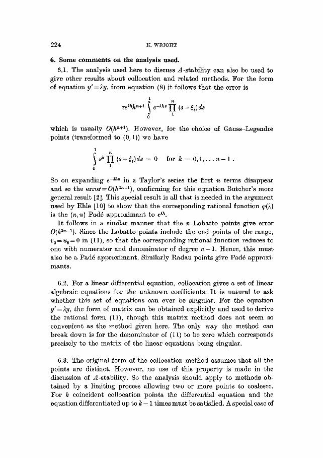
6.1. The analysis used here to discuss A-stabi~ty can also be used to give other results about collocation and related methods. For the form of equation y'=,~y, from equation (8) it follows tha t the error is

1

Te~h~+1 e-~hs I I (8- ~t) d8 1

0

which is usually O(hn+l). However, for the choice of Gauss-Legendre points (transformed to (0, 1)) we have

1

i s k r I ( s - ~ i ) d s = 0 for k = 0,1 . . . . n - 1 . d 1 o

So on expanding e -~h8 in a Taylor's series the first n terms disappear and so the error= O(h2n+l), confirming for this equation Butcher's more general result [2]. This special result is all that is needed in the argument used by Ehle [10] to show that the corresponding rational function ~(2) is the (n, n) Padd approximant to e ~h.

I t follows in a similar manner tha t the n Lobatto points give error O(h~-l). Since the Lobatto points include the end points of the range, Vo = *~0 = 0 in (11), so tha t the corresponding rational function reduces to one with numerator and denominator of degree n - 1. Hence, this must also be a Padd approximant. Similarly Radau points give Pad~ approxi- mants.

6.2. For a linear differential equation, collocation gives a set of linear algebraic equations for the unknown coefficients. I t is natural to ask whether this set of equations can ever be singular. For the equation y'= ]ty, the form of matrix can be obtained explicitly and used to derive the rational form (1 I), though this matrix method does not seem so convenient as the method given here. The only way the method can break down is for the denominator of (11) to be zero which corresponds precisely to the matrix of the linear equations being singular.

6.3. The original form of the collocation method assumes tha t all the points are distinct. However, no use of this property is made in the discussion of A-stability. So the analysis should apply to methods ob- tained by a limiting process allowing two or more points to coalesce. For k coincident collocation points the differential equation and the equation differentiated up to k - 1 times must be satisfied. A special case of

S O M E R E L A T I O N S H I P S B E T W E E N I M P L I C I T R U N G E - K U T T A . . . 225

this is the Taylor's series method when all the points are taken at the beginning of the range. If the points are taken at the two ends of the range one obtains a method similar to those discussed by Makinson [13].

7. Conclusions.

The analysis given shows tha t the A-stability of a collocation or equiv- alent method can easily be tested in practice. Clearly, whether the condi- tions are satisfied or not depends on the distribution of the collocation points, but it is not clear whether this can be related to any simple geometric or other property of the distribution in more than a general way.

Osborne [15] has pointed out tha t in certain circumstances more strin- gent conditions than those provided by A-stability may be desirable. In particular it might be required tha t as ~ -~ ~ , ~(A)Should tend to a limit definitely less than one. One consequence of this is tha t some increasing functions will be represented by decreasing ones. However, for formulae based on symmetric points, ~(A)= 1/~v(-4) so tha t decreasing functions are represented by decreasing functions and increasing hmetions by in- creasing ones, as long as the A-stability conditions hold.

The results for the Gauss-Legendre formula seem very neat, and it is natural to speculate whether the same holds true for Chebyshev zeros or extrema. However, the results for small numbers of points are perhaps more important in practice, as the size of the set of algebraic equations needing solution could become prohibitive for a formula using a large number of points, particularly if it is applied to a large set of simultaneous ordinary differential equations.

The method used here for the discussion of the A-stability of colloca- tion and related methods would clearly apply to other methods for which ~v(2) is a rational function of ~ as long as the coefficients of the rational function can be evaluated in some way.

A P P E N D I X

A-Stabi l i ty of formula using n Gauss Points.

In this case the pol)~nomial whose zeros we wish to examine has co- efficients which can be found explicitly, as they are related to the Le- gendre polynomial.

I t follows that

~ r! v~#r = const. ~ (n+r)! r o o ( n - r ) ! r ! ~ "

2 2 6 K. W R I G H T

Now in the Routh-Hurwi tz algorithm two rows of an array {aj k} are formed first. They consist of alternate coefficients of this polynomial, tha t is

(2n-- 2r) ! ~ r ° = r = 0 , . . . n + 2

(2r) ! (n-- 2r)!

0¢r 1 _-- ( 2 n - 2 r - 1)!

(2r+ 1)! (n-2r- 1)! r = 0 . . . . ( n - l ) + 2

where the symbol + is the integer divide as used in Algol. The Routh- t turwi tz Algorithm then forms further rows of ar k defined

b y 0¢k-2

k 0/k--2 0 k--I 0% = r + i - - ~ O~r+i, r = 0 . . . . ( n - k - I ) + 2 o; 0

o~k _ ~k-2 and, if n - k is even, (n-~)/2- (~-k)/2+1" I t then follows by induction tha t

( 2 n - 2 r - - 1)! ( r + k - 1 ) ! (n-r-k)! ark = ( 2 r + 2 k - 1 ) ! (n-2r-k)! ( n - r - l ) ! r!' r = 0 , . . . ( n - k ) + 2 .

The Algorithm then requires tha t all the values of a0 k, k -- 0 , . . . n shall have the same sign, which is easily seen.

REFEREI~CES

i. O. Axelsson, A Class of A-S~ble Methods, BIT 9 (1969), 185-199.

2. ft. C. Butcher, Implicit Runge-Kutta Processes, Math. Comp. 18 (1964), 50-64. 3. J . C. Butcher, Integration Processes Booed on Raclau Quadrature Formulas, Math.

Comp. 18 (1964), 233-244. 4. L. Collatz, The Numerical Treatment of Differential Equations, (2nd English Ed.)

Springer, Berlin (1960). 5. G. J . Cooper, Interpolation and Quadrature Methods for Ordinary Differential Equa.

tions, Math. Comp. 22 (1968), 69-73. 6. C. F. Curtiss and J . O. :Hirschfelcter, Integration of Stiff Equations, Proc. Nat . Aead.

Sci. U.S. (1952), 235-243. 7. G. G. Dahlquist , A special stability problem for linear multistep methods, BIT 3 (1963),

27-43. 8. B. L. Ehle, High Order A-Stable Methods for the Numerical Solution of Systems of Dif-

ferential Equations, BIT 8 (1968), 276-278. 9. F. 1%. Gantmacher , Matrix Theory, Vol. I I , Chelsea, New York (1959).

10. C. W. Gear, The Automatic Integration of Stiff Ordinary Differential Equations, Proc. I .F.I .P. Congress (preprint) (1968), A81-A85.

11. C. Lanczos, Trigonometric Interpolation of Empixical and Analytical Functions, J. Math. Phys. 17 (1938), 123-199.

SOME RELATIONSHIPS B E T W E E N IMPLICIT RUNGE-KUTTA . . . 227

12. C. Lanczos , Tables of Chebyshev Polynomials ( In t roduc t ion ) , Na t . Bur . S t a n d . Appl .

Ma th . Ser. 9 (1952). 13. G. J . Makinson , Stable High Order Implicit Methods for the Numerical Solution of

Systems of Differential Equations, Comp. J . 11 (1968), 305-310. 14. H . Mineur , Techniques de Caleul ~'umerique, Beranger , P a r i s (1952).

15. M. R . Osborne , A New Method for the Integration of St i f f Systems of Ordinary Differen- tial Equations, Proc. I F I P Congress (prelorint) (1968), A86-A90 .

COMPUTING LABORATORY UNIVERSITY OF NEWCASTLE UPON TYNE ENGLAND