some studies on minimal and non-minimal universal extra
TRANSCRIPT

Some studies on Minimal
and Non-minimal
Universal Extra Dimension
by
Ujjal Kumar Dey
Enrolment Number : PHYS08200605001
Harish-Chandra Research Institute, Allahabad
A Thesis submitted to theBoard of Studies in Physical Science Discipline
in partial fulfillment of the requirementsfor the degree of
DOCTOR OF PHILOSOPHYof
Homi Bhabha National Institute
October, 2014


Statement by author
This dissertation has been submitted in partial fulfillment of requirements for an ad-vanced degree at Homi Bhaba National Institute (HBNI) and is deposited in the Libraryto be made available to borrowers under rules of the HBNI.
Brief quotation from this dissertation are allowable without special permission, pro-vided that accurate acknowledgement of source is made. Requests for permission forextended quotation from or reproduction of this manuscript in whole or in part may begranted by the Competent Authority of HBNI when in his or her judgment the proposeduse of the material is in the interests of scholarship. In all other instances, however, per-mission must be obtained from the author.
Date: Ujjal Kumar Dey
(Ph. D. Candidate)


Declaration
I, hereby declare that the investigation presented in the thesis has been carried out byme. The work is original and has not been submitted earlier as a whole or in part for adegree/diploma at this or any other Institution/University.
Date: Ujjal Kumar Dey
(Ph. D. Candidate)


Certificate
This is to certify that the Ph.D. thesis entitled Some studies on Minimal and Non-minimal Universal Extra Dimension submitted by Ujjal Kumar Dey for the award ofthe degree of Doctor of Philosophy is a record of bona fide research work done undermy supervision. It is further certified that the thesis represents the independent workdone by the candidate and collaboration was necessitated by the nature and scope of theproblems dealt with.
Date:
Biswarup Mukhopadhyaya
(Thesis Supervisor)


List of publications arising from the thesis
Journals
1. “Boundary localized terms in universal extra-dimensional models through a darkmatter perspective",A. Datta, U. K. Dey, A. Raychaudhuri and A. Shaw,Phys. Rev. D 88, 016011 (2013).
2. “Constraining minimal and nonminimal universal extra dimension models withHiggs couplings",U. K. Dey and T. S. Ray,Phys. Rev. D 88, 056016 (2013).
3. “KK-number violating decays: Signal of n = 2 excitations of Extra-DimensionalModels at the LHC",U. K. Dey and A. Raychaudhuri,arXiv:1410.1463 [hep-ph],Nucl. Phys. B 893, (2015) 408-419
Conferences
1. “Universal Extra-Dimensional models with boundary terms: Probing at the LHC",A. Datta, U. K. Dey, A. Raychaudhuri and A. Shaw,Nucl. Phys. Proc. Suppl. 251-252, (2014) 39-44.
2. “Universal extra dimensions : life with BLKTs",A. Datta, U. K. Dey, A. Raychaudhuri and A. Shaw,J. Phys. Conf. Ser. 481, (2014) 012006.
Ujjal Kumar Dey
(Ph. D. Candidate)


To
My Mother


Acknowledgments
I would like to thank Prof. Biswarup Mukhopadhyaya for supervising my thesis work.I have learned a lot from him. His guidance and help at various stages played a pivotalrole in the completion of my thesis work.
I would like to express my profound gratitude to my collaborator and mentor Prof.Amitava Raychaudhuri for his guidance and continuous support throughout my Ph. D.life. His immense patience, deep knowledge, encouragement to think and work indepen-dently catalyze my transition from a student to a researcher.
I am grateful to my collaborator Prof. Anindya Datta, from whom I learned variousaspects of extra dimensions. I would like to thank Avirup Shaw for his diligence andsincerity during our collaboration. I enjoyed working with Tirthada (Tirtha Sankar Ray).He has this brilliant capability of coming up with a solution to any problem. I would liketo acknowledge the wonderful experience that I have working with my friend Dipankarand brother-like junior Landau (Nabarun).
I am thankful to the past and present members of the particle physics phenomenol-ogy group at the Harish-Chandra Research Institute (HRI), Prof. Raj Gandhi, Prof. AseshK. Datta, Prof. V. Ravindran, Prof. Sandhya Choubey, Dr. Santosh Rai, Dr. AndreasNyffeler from whom I learned many aspects of high energy physics. The physics discus-sion sessions at the Pheno-Lunch was an exciting way to remain updated on the recentdevelopments of the subject.
I am deeply indebted to the faculty members of HRI for creating an excellent environ-ment for learning through various course works and projects. I take this opportunity tothank Prof. Ashoke Sen, Prof. Rajesh Gopakumar, Prof. L. Sriramkumar, Prof. Satchi-dananda Naik, Prof. Dileep Jatkar, Prof. Pinaki Majumdar, Prof. Sudhakar Panda, Prof.Tapas K. Das and Prof. J. S. Bagla. I would also like to acknowledge Anirbanda (Dr.Anirban Basu) for his candid friendship with all of us students. I am also thankful to thefaculty members of University of Calcutta where a large part of my thesis work has beendone. Especially I am grateful to Prof. Anindya Datta and Prof. Anirban Kundu.
The administration at HRI has always been very helpful and efficient. I would like toexpress my gratitude to all the non-academic members of this institute for their help andsupport at every stage. The workers and staffs are also acknowledged for always beingready at their services.

A very special thanks to my batch-mates at HRI. The life at HRI would not have beenthe same without them. Thank you Bhuruda (Sourav Mitra), Thikaa (Saurabh Niyogi),Manojda, Rambha (Saurabh Pradhan), Arunabhada, Taratda and Vikas for all the happymoments that we shared together throughout our journey in the Ph. D. life. I will alwayscherish those memories.
I am very grateful to my seniors at HRI. At each step their help and support takeme through many difficult situations. Arjunda, Shubhoda, Shamikda, Soumyada, Kaka(Kirtimanda), Joydeepda, Sanjoyda, Dhirajda, Satyada, Atrida, Arijitda, Arindamda,Arghyada, Ambreshji, Kenji – thank you all. I am deeply indebted my other friends –Shankha, Tanumoyda and Animeshda. The void created by the leaving of the seniorsare beautifully filled up by the set of juniors and in no time they became close friends.Thanks Aritra, Dibya, Rana, Taushif, Titas, Soumyarup, Arijit, Tamoghna, Sauri, Swap-namay, Masud, Avijit, Avishek, Nyaya for keeping a vibrant and lively campus life. Iwill miss the late night long refreshing tea sessions at the guest house where all possi-ble topics of the Universe were discussed among the friends with ardent zeal. I am alsothankful to Paromitadi, Anushreedi and Ushoshi. As I have spent a considerable part ofmy Ph. D. life at the University of Calcutta, I would like to thank all of my friends there.Special thanks to T. K. Bose, Kartick, Khaleque, Swarupda and Shirshenduda for makingthe otherwise mundane stay at Kolkata a very lively one. I am deeply grateful to Kalida(Kalipada Das) for providing me shelter whenever I had to stay at Kolkata.
Evidently for the remaining of my life I can safely presume that I would be able to saythat "...those were the best days of my life".
Finally, I am indebted beyond measure to all my family members for their love andconstant support. Special thanks to Chunilal Das, Shankar Chandra Dey and Arun KumarPan for shaping me from the very beginning of my academic life and being constantsource of inspiration.
Thank you all...

Contents
Synopsis iii
List of tables vii
List of figures ix
1 Universal Extra Dimension 11.1 Introduction . . . . . . . . . . . . . . . . . . . . . . . . . . . . . . . . . . . . . 11.2 Standard Model and beyond . . . . . . . . . . . . . . . . . . . . . . . . . . . . 1
1.2.1 Particle content and interactions . . . . . . . . . . . . . . . . . . . . . 31.2.2 Brout-Englert-Higgs mechanism . . . . . . . . . . . . . . . . . . . . . 51.2.3 A few shortcomings of SM . . . . . . . . . . . . . . . . . . . . . . . . 8
1.3 Extra Dimension . . . . . . . . . . . . . . . . . . . . . . . . . . . . . . . . . . 101.3.1 Large Extra Dimension . . . . . . . . . . . . . . . . . . . . . . . . . . . 111.3.2 Warped Extra Dimension . . . . . . . . . . . . . . . . . . . . . . . . . 12
1.4 Universal Extra Dimension . . . . . . . . . . . . . . . . . . . . . . . . . . . . 121.4.1 Basic features . . . . . . . . . . . . . . . . . . . . . . . . . . . . . . . . 131.4.2 KK parity . . . . . . . . . . . . . . . . . . . . . . . . . . . . . . . . . . 171.4.3 Standard Model in 5D . . . . . . . . . . . . . . . . . . . . . . . . . . . 171.4.4 Particle content and interactions . . . . . . . . . . . . . . . . . . . . . 19
1.5 Structure of this thesis . . . . . . . . . . . . . . . . . . . . . . . . . . . . . . . 21
2 Minimal and Non-minimal Universal Extra Dimension 232.1 Minimal Universal Extra Dimension . . . . . . . . . . . . . . . . . . . . . . . 23
2.1.1 Radiative corrections . . . . . . . . . . . . . . . . . . . . . . . . . . . . 232.1.2 Mass spectrum . . . . . . . . . . . . . . . . . . . . . . . . . . . . . . . 26
2.2 Non-minimal Universal Extra Dimension . . . . . . . . . . . . . . . . . . . . 27
i

CONTENTS
2.2.1 Model description . . . . . . . . . . . . . . . . . . . . . . . . . . . . . 28
3 Dark Matter & Non-minimal Universal Extra Dimension 353.1 Dark Matter . . . . . . . . . . . . . . . . . . . . . . . . . . . . . . . . . . . . . 35
3.1.1 Evidences . . . . . . . . . . . . . . . . . . . . . . . . . . . . . . . . . . 353.1.2 Basic properties . . . . . . . . . . . . . . . . . . . . . . . . . . . . . . . 373.1.3 A few candidates . . . . . . . . . . . . . . . . . . . . . . . . . . . . . . 38
3.2 Relic density . . . . . . . . . . . . . . . . . . . . . . . . . . . . . . . . . . . . . 403.2.1 Standard calculation of relic density . . . . . . . . . . . . . . . . . . . 403.2.2 Coannihilation . . . . . . . . . . . . . . . . . . . . . . . . . . . . . . . 43
3.3 Relic density in mUED and nmUED . . . . . . . . . . . . . . . . . . . . . . . 443.3.1 mUED . . . . . . . . . . . . . . . . . . . . . . . . . . . . . . . . . . . . 443.3.2 nmUED . . . . . . . . . . . . . . . . . . . . . . . . . . . . . . . . . . . 46
3.4 Direct Dark Matter Detection in mUED and nmUED . . . . . . . . . . . . . . 533.4.1 mUED . . . . . . . . . . . . . . . . . . . . . . . . . . . . . . . . . . . . 553.4.2 nmUED . . . . . . . . . . . . . . . . . . . . . . . . . . . . . . . . . . . 56
3.5 Summary and Conclusions . . . . . . . . . . . . . . . . . . . . . . . . . . . . 60
4 Non-minimal Universal Extra Dimension Confronting Higgs Data 654.1 Loop-induced Higgs couplings . . . . . . . . . . . . . . . . . . . . . . . . . . 664.2 mUED results . . . . . . . . . . . . . . . . . . . . . . . . . . . . . . . . . . . . 674.3 nmUED results . . . . . . . . . . . . . . . . . . . . . . . . . . . . . . . . . . . 694.4 Conclusion . . . . . . . . . . . . . . . . . . . . . . . . . . . . . . . . . . . . . . 73
5 Signal of Second Level Kaluza-Klein Particles 755.1 Coupling of the 2n-level top quark to zero mode states . . . . . . . . . . . . 765.2 Decays of a 2n-level top quark . . . . . . . . . . . . . . . . . . . . . . . . . . . 795.3 Detection prospect of the n = 2 top quark . . . . . . . . . . . . . . . . . . . . 805.4 Conclusion . . . . . . . . . . . . . . . . . . . . . . . . . . . . . . . . . . . . . . 83
6 Summary and conclusions 85
ii

SYNOPSIS
The Standard Model (SM) is by far the most successful model of particle physics. Veryrecently the discovery of the Higgs particle and other observations at LHC augment thisfact. Even after the immense success of SM the reticence of it to provide us with theanswer to some aesthetic (Gauge coupling unification, hierarchy problem etc.) and com-pelling questions (massive neutrinos, baryon asymmetry, dark matter (DM) etc.) leadsus to think beyond SM (BSM). Supersymmetry (SUSY) and Extra Dimensional (ED) the-ories are two strong proponents to solve some of these problems. A particular variant ofED models is Universal Extra Dimensional (UED) models where all the Standard Model(SM) fields can access one or more extra spatial dimensions. The simplest case can beof one extra dimension. The extra spatial dimension must be compactified at a scale1/R ∼ O(TeV), where R is the compactification radius. To get chiral fermions, orb-ifold compactification is needed. Although orbifolding breaks 5D translational invariancethere remains a residual symmetry, called KK-parity, responsible for the stability of thelightest Kaluza-Klein particle (LKP). In the effective four dimensional theory there will betowers of heavy Kaluza-Klein (KK) modes for each SM field. The masses of these heavymodes depend on the compactification scale. For a specific level the mass spectrum isthus almost degenerate. But radiative corrections lift this degeneracy. Without violatingthe 4D symmetries of SM, additional interaction terms between the KK modes can bewritten at the fixed points of the orbifold. Such terms can also creep in as counterterms tocompensate for radiative effects of the 5D theory. In minimal UED (mUED) these termsare chosen in such a way that the 5D loop contributions are exactly compensated at thecut-off scale. Being a 5D quantum field theory, mUED is non-renormalisable and shouldbe considered as an effective field theory and valid up to some high energy scale. Thisis why one should not discard a priori any operator that is allowed by 4D Lorentz invari-ance and SM gauge invariance. Boundary localised terms (BLTs) are such operators. Thescenario with arbitrary non-vanishing BLTs is termed as non-minimal UED (nmUED).
Even after conclusive evidence of existence of DM, the actual identity of DM is stillunknown. In the context of mUED, the first KK level photon γ(1), being the LKP and thushaving the required stability governed by the conservation of KK parity, can be a goodcandidate for DM. In nmUED the mass spectrum is determined by the BLT parameters

SYNOPSIS
and thus depending on them the identity of LKP can be changed. The existence of stableLKP in nmUED is possible only when there are equal strength BLTs at two boundaries.In the first study, we considered the possibility of various possible LKPs. In each case wecalculated the relic density following the standard procedure of solving Boltzmann equa-tion with appropriate assumptions. Co-annihilation, which is a necessary considerationfor near degenerate mass spectra, has also been taken into account. We have derived allthe necessary cross sections analytically, using CalcHEP. We used direct detection datafrom XENON100 to constrain the parameter space. We found for specific choice of pa-rameters, not only γ(1) can be a good DM candidate but also the narrow bounds on com-pactification scale from similar studies in mUED can be evaded. We also found that thefirst level Z-boson, with mass at TeV range, can not be a single component DM candidateas it does not meet the criteria for appropriate relic density.
The tour de force of LHC is the discovery of Higgs particle, till date. Apart from mea-suring its mass, LHC data finds a few discrepancies in the Higgs couplings. For example,global analysis of ATLAS and CMS data showed that there is slight excess in H → γγ
(which is actually a loop-induced process) decay rate from the SM prediction. However,these deviations sustained even after the refined analysis of available data. It is possiblethat this excess is due to some new physics. The heavier new particles can leave theirfootprints in loop-induced processes where they can come as virtual intermediate parti-cles. In this way, heavier KK modes can alter various loop-induced decay processes ofHiggs and we can compare between this alteration and observed data. In this spirit, inthe second work we showed that the present data disfavors new physics scale below 1.3TeV with 95% confidence level for the mUED. However, we showed that a more generalscenario in nmUED can accommodate scales as low as 0.4 TeV.
In the simplest UED models KK parity distinguishes the states with odd and evenKK-number. As has already been mentioned, the KK-excitations of all SM particles atany KK-level n are degenerate in mass which is lifted by mUED radiative corrections.In the third work, in preparation, we focused our attention on the KK-parity conservingcoupling of a 2n-level KK top quark to the n = 0 top quark and an n = 0 Higgs boson.Since mUED interactions are KK-number conserving this coupling will be loop induced.We compare the decay mediated by this coupling with the KK-number conserving decayto two n-level states which proceeds through tree-level couplings. The latter process isphase space suppressed and becomes allowed only after mUED corrections are incorpo-rated. As an application of this result we have examined the prospect of pair producingn = 2 level KK top-antitop quarks at the LHC with
√s = 13 TeV and 33 TeV and examine
iv

SYNOPSIS
the prospects of the detection of both of them in the above mentioned decay mode.
v

List of Tables
3.1 The B(1) annihilation and relevant B(1)-lepton scattering process that areimportant for the relic density calculation of B(1). . . . . . . . . . . . . . . . 49
3.2 The ν(1) and `(1) annihilation and scattering processes which contribute tothe relic density calculation. . . . . . . . . . . . . . . . . . . . . . . . . . . . . 49
3.3 The ν(1)-`(1) scattering processes which contribute to the relic density cal-culation. . . . . . . . . . . . . . . . . . . . . . . . . . . . . . . . . . . . . . . . 50
3.4 Upper bound on R−1 from overclosure of the universe (Ωh2 = 0.48). Themasses of the LKP for the limitingR−1 are also presented. For theW (1)
3 LKPcase only the processW (1)
3 W(1)3 → W+ W− is taken into account. Including
coannihilation will further enhance the upper bound in this case. . . . . . . 52
vii


List of Figures
1.1 Particle content of the SM. . . . . . . . . . . . . . . . . . . . . . . . . . . . . . 4
1.2 The Higgs potential in the SM (taken from [19]). . . . . . . . . . . . . . . . . 7
1.3 Pictorial description of orbifolding. . . . . . . . . . . . . . . . . . . . . . . . . 15
2.1 An example of a loop winding around the extra dimension. . . . . . . . . . 24
2.2 (From [58]). Particle spectrum for the first level KK particles at tree level(left) and after one loop correction (right). Assuming Higgs massmH = 120
GeV, 1/R = 500 GeV and ΛR = 20. . . . . . . . . . . . . . . . . . . . . . . . . 27
2.3 Variation of M (1) = m1R with BLT strength RBLT = r/R. Larger RBLT
yields a smaller mass. This result applies to any type of fields when theircorresponding BLTs are symmetric. . . . . . . . . . . . . . . . . . . . . . . . . 32
3.1 The observed rotation curve of the dwarf spiral galaxy M33. The dashedline is predicted purely on the basis of luminous stellar disc. The observedcurve is flatter than the predicted one. This suggests the presence of a haloof dark matter, extending to large galactic radii. (From [77]). . . . . . . . . . 36
3.2 Relic density of LKP (i) γ(1) (left) and (ii) Z(1) (right) as a function of LKPmass. The green band gives 2σ allowed region from WMAP 5yr data [130],ΩCDMh
2 ∈ (0.1037, 0.1161) and the vertical cyan band excludes the massof LKP from precision data. Here KK singlet and doublet quarks are as-sumed to be degenerate and the mass of the level one quarks are varied byhand, such that ∆q1 = 0.01, 0.02, 0.05, 0.1 and 0.5. Also Z(1) and W (1)± aretaken to be degenerate. The red dotted line gives the result of full mUEDcalculation including all coannihilation processes. Adapted from [117]. . . . 46
ix

LIST OF FIGURES
3.3 Variation of Ωh2 with relic particle mass, mB(1) . Curves for different choicesof the fermion BLKT parameter Rf are shown and the corresponding ∆f
indicated. The narrow horizontal blue band corresponds to the 1σ allowedrange of relic particle density from Planck data [74]. The allowed 1/R (ormB(1)) can be read off from the intersections of the curves with the allowedband. The three panels are for different choices of RB, the BLKT parameterfor B. . . . . . . . . . . . . . . . . . . . . . . . . . . . . . . . . . . . . . . . . . 51
3.4 Allowed region in the mf (1) − mB(1) plane that satisfies the observed Ωh2
limits. The three panels are for different choices of RB. Only the narrowstrip between the two curves is allowed from the relic density constraints. . . 52
3.5 Variation of the relic density withmW
(1)3
in the case ofW (1)3 LKP. The current
observed value (∼ 0.12) disfavors this alternative. . . . . . . . . . . . . . . . 53
3.6 Schematic presentation of DM interaction (taken from [131]). . . . . . . . . . 54
3.7 Spin dependent and scalar LKP-nucleon cross section as a function of B(1)
mass for ∆q(1) = 5, 10, 15% and mH = 120 GeV. Adapted from [109]. . . . . 56
3.8 The Feynman diagrams for B(1) and quark scattering. . . . . . . . . . . . . . 58
3.9 Variation of the scalar B(1)-nucleon cross section with relic particle massfor Xenon. The three panels are for three values of RB. The shaded (blue)region represents the cross section for a continuous variation of Rq withinthe range bounded by the two curves. . . . . . . . . . . . . . . . . . . . . . . 59
3.10 Variation of the spin dependent B(1)-nucleon cross section with relic par-ticle mass for Xenon. The three panels are for three values of RB. Theshaded (blue) region shows the cross section for a continuous variation ofRq within the range bounded by the two curves. . . . . . . . . . . . . . . . . 59
4.1 The ratios of the Higgs couplings in UED scenario to their SM values areplotted as functions of the inverse radius of compactification of the extradimension (1/R). The blue (shaded) bands represent the 95% confidencelevel allowed values for these ratios [156], with the red (solid) horizontallines representing the central values from LHC data. The blue (dashed)lines correspond to the SM points. The black (dark) curves are the UEDpredictions. We have assumed mH = 125 GeV. . . . . . . . . . . . . . . . . . 69
x

LIST OF FIGURES
4.2 The ratios of the Higgs couplings in the BLKT scenario to their SM valuesare plotted as functions of the inverse radius of compactification of the ex-tra dimension (1/R). The blue (shaded) bands represent the 95% confidencelevel allowed values for these ratios [156], with the red (light) horizontallines representing the central values from LHC data. The blue (dashed)lines correspond to the SM points. The black (dark) points represent theBLKT results. We have assumed mh = 125 GeV. The BLKT parameters rQand rY are varied within the range [−πR/2, πR/2]. . . . . . . . . . . . . . . . 72
5.1 The dominant diagrams in the unitary gauge generating an effectivet(2n)L t
(0)R H(0) coupling. . . . . . . . . . . . . . . . . . . . . . . . . . . . . . . . . 77
5.2 The branching ratio for the process t(2) → t(0)H(0) as a function of ΛR. Thered solid (blue dot-dashed) curve is for t(2)
L (t(2)R ) decay. . . . . . . . . . . . . 80
5.3 The production cross section for a t(2)t(2) pair at the LHC. The blue solid(red dashed) curve corresponds to
√s = 13 TeV (33 TeV). . . . . . . . . . . . 81
5.4 The cross section for the (tH)(tH) signal at the LHC as a function of thet(0)H(0) invariant mass. The histograms for different choices of 1/R (ex-plained in the legend) and the SM background (shown shaded) at the LHCrunning at
√s = 13 TeV (left) and 33 TeV (right). . . . . . . . . . . . . . . . . 82
xi


Chapter 1
Universal Extra Dimension
1.1 Introduction
In this chapter we will set the notations and conventions required for the later chapters.We will discuss extra-dimensional theories, with a special emphasis on universal extradimensional model which, along with some variants of it, is the main topic of interest inthis thesis. Before delving into the extra dimensions it would not be out of place to recallthe most successful theory of elementary particles, the Standard Model (SM). In Sec. 1.2we revisit the SM and in subsequent Secs. 1.3 and 1.4 we will give a brief introduction toextra dimensions.
1.2 Standard Model and beyond
The Standard Model (SM) of particle physics epitomizes our current understanding of thebasic building blocks of the universe. These basic building blocks are elementary particleswhich are fundamental, in the sense that they are indivisible and have no sub-structure.SM is a theory of three of the four fundamental forces of Nature, namely electromag-netic, weak and strong interactions (gravity is not included in the paradigm of SM) thatsuperintend the dynamics of these particles. The matter of the universe is composed offermionic fields and the interaction between them is governed by the bosonic fields. InSM we have three types of particles: spin-1/2 fermions, spin-1 gauge bosons and a spin-0scalar field, Higgs boson. SM is a quantum field theory (QFT) based on various symme-tries. Actually QFT is the result of the combination of quantum mechanics and specialtheory of relativity. SM possesses the following symmetries.
(i) Lorentz symmetry : This is a space-time symmetry. The manifestation of Lorentz
1

CHAPTER 1. UNIVERSAL EXTRA DIMENSION
symmetry is that the laws of nature are independent of rotations and boosts. Thefields (elementary particles are described by fields in QFT) of SM have definite trans-formation properties depending on their spins. Lorentz invariance is a symmetryof the Lagrangian describing the theory. If the Lagrangian transforms as a scalarunder the Lorentz transformations then the theory is said to be Lorentz invariant.As it stands SM is manifestly Lorentz invariant.
(ii) Gauge symmetry : Gauge transformations are local transformations of the fields.Actually the interactions among matter fields, i.e., the fermionic fields and gaugefields are described by the principle of local gauge invariance. The gauge group ofthe SM is SU(3)c⊗SU(2)L⊗U(1)Y which dictates the three fundamental interactionsof Nature. The strong interactions are described by the SU(3)c gauge group whereasSU(2)L ⊗U(1)Y accounts for the electroweak (EW) interactions. This EW symmetrybreaks to the electromagnetic symmetry, U(1)em via the Brout-Englert-Higgs (BEH)mechanism with the help of a scalar field which is called Higgs field.
(iii) Discrete symmetry : There are discrete transformations that arise in QFT. Chargeconjugation (C), parity transformation (P ) and time reversal (T ) are examples ofsuch transformations. Among these P and T are just the subset of Lorentz transfor-mations. Actually P and T are discrete Lorentz transformations. The action of P isto reflect the spatial coordinates (e.g., ~x → −~x) which ultimately results in a flip inchirality (handedness) of the field. The operation of T is just to flip the direction oftime. The effect of C is to interchange the particle to its antiparticle and vice-versa.The electromagnetic interaction is invariant under C, P, and T . The electroweakinteraction violates both C and P . Thus, individually none of these are good sym-metries of SM. However, the combined operation CPT is always conserved in anystandard QFT1.
(iv) Global symmetry : SM also has two accidental global symmetries: baryon number(B) and lepton number (L). However, they can be violated by quantum effects.These type of symmetries which are conserved classically but violated via quan-tum effects are called anomalous. It is worth mentioning that (B − L) is still a goodsymmetry of SM and is not anomalous.
Apart from these symmetries there are some other important aspects of SM. It is arenormalizable theory, i.e., all the ultra-violet (UV) divergences that can arise from higher
1See [1] for a proof of CPT -theorem.
2

1.2. STANDARD MODEL AND BEYOND
order quantum effects can be removed by judicious redefinition of bare fields and param-eters of the model. Unitarity, i.e., the conservation of probability in various interactionprocesses, and the stability of EW vacuum are two other important facets of SM.
1.2.1 Particle content and interactions
We have already mentioned that the matter of the universe is made up of spin-1/2fermions. Among these there are six types of quarks and six types of leptons (three elec-trically charged and three neutral). The transformation properties of these fields underSM gauge group are determined by their respective charges under the gauge groups. Thequark fields transform as triplets (fundamental representation) of SU(3)c, whereas the lep-tons are singlet under this gauge group and have no color charge and consequently donot take part in strong interactions. SM being a chiral theory, treats left-handed and right-handed fields differently. The left-handed2 fields transform as doublets (fundamentalrepresentation) under SU(2)L while the right-handed fields are singlets under this group.Thus we have for quarks,
Doublets :
(u
d
)
L
,
(c
s
)
L
,
(t
b
)
L
Singlets : uR, dR, cR, sR, tR, bR.
For leptons we have,
Doublets :
(νe
e
)
L
,
(νµ
µ
)
L
,
(ντ
τ
)
L
Singlets : eR, µR, τR.
Note that there is no right-handed neutrino in SM3. The SU(2)L group has three genera-tors constructed out of the three Pauli matrices, σa (a = 1, 2, 3). If T3 be the eigenvalueof the third generator and Q be the electric charge of the field, then the transformationof that field under the U(1)Y is determined by the quantum number called hyperchargewhich is defined as,
Q = T3 +Y
2. (1.1)
2The left-handed projection of a field ψ is defined as ψL = PLψ = [(1−γ5)/2]ψ and for the right-handedone, ψR = PRψ = [(1 + γ5)/2]ψ.
3In SM the neutrinos are massless particles. But recent neutrino experiments show that they have tinymasses. Some extensions of SM add right-handed neutrinos to explain the mass of the neutrinos.
3
CHAPTER 1. UNIVERSAL EXTRA DIMENSION
With this convention the lepton doublets will have hypercharge (−1), and for leptonsinglets it is (−2). The quark doublets are of hypercharge +1/3 and up-type quark singletsit is +4/3 and down-type quark singlets will have hypercharge (−2/3).
With the knowledge of the transformation property of the fields under SM gaugegroup one can write the gauge invariant Lagrangian of the theory. The kinetic term4
for the fermionic fields (ψ) can be written as,
Lmatter = iψ /Dψ = iψγµDµψ, (1.2)
where the most general form of the covariant derivative Dµ is given by,
Dµ = ∂µ − ig1Y
2Bµ − ig2
σa
2W aµ − ig3
λi
2Giµ, (1.3)
where g1, g2 and g3 are the gauge couplings for U(1)Y , SU(2)L and SU(3)c groups respec-tively. It should be noted that if a field transforms as a singlet under a specific gaugegroup then that specific gauge coupling will be zero for that field. Here Bµ is the gaugefield for U(1)Y , W a
µ (a = 1, 2, 3) are for SU(2)L and Giµ (i = 1, 2, . . . , 8) for SU(3)c group.
Substituting this form of Dµ in Eq. 1.2 one can obtain the interaction vertices between thefermions and the gauge bosons.
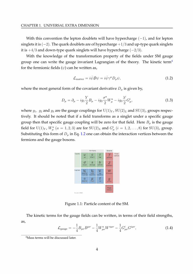
Figure 1.1: Particle content of the SM.
The kinetic terms for the gauge fields can be written, in terms of their field strengths,as,
Lgauge = −1
4BµνB
µν − 1
4W aµνW
aµν − 1
4GiµνG
iµν , (1.4)
4Mass terms will be discussed later.
4
1.2. STANDARD MODEL AND BEYOND
where the field strength tensors are defined as,
Bµν = ∂µBν − ∂νBµ, (1.5a)
W aµν = ∂µW
aν − ∂νW a
µ + g2εabcW b
µWcν , (1.5b)
Giµν = ∂µG
iν − ∂νGi
µ + g3fijkGj
µGkν , (1.5c)
where εabc and fabc are the structure constants of SU(2)L and SU(3)c groups respectively.Thus from the kinetic terms it is evident that for non-Abelian gauge fields there existstriple and quartic self-interaction vertices.
We have talked about the kinetic terms of fermions and gauge bosons. Actually gaugesymmetry forbids any kind of mass terms for gauge fields. But it is an established fact thatthe weak interaction mediator gauge bosons, W± and Z-bosons are massive. Moreover,the incongruity in the transformation properties of the left-handed and right-handedfermions prohibits gauge invariant mass term for fermions also. These facts lead us tothink that the electroweak gauge symmetry must be broken. The introduction of the con-cept of spontaneous symmetry breaking (SSB) [2–10] helps to reconcile these mass relatedissues. The crux of this SSB is that the Lagrangian of the theory is invariant under thegauge transformations but the vacuum does not respect that symmetry. The electroweaktheory, also known as Glashow-Salam-Weinberg model [11–13] incorporates SSB by intro-ducing a spin zero complex scalar field, called Higgs field, which transforms as doubletunder SU(2)L and takes appropriate vacuum expectation value (vev) to break the gaugesymmetry spontaneously. As a consequence of this breaking the fermions and the gaugebosons can obtain masses. The SM particle zoo has been shown in Fig. 1.1. It is worthmentioning that the spontaneously broken gauge theory is also renormalizable [14, 15].In the next subsection we are going to describe the mechanism in a nut shell.
1.2.2 Brout-Englert-Higgs mechanism
We have already mentioned that to explain the masses for the W± and Z bosons andfermions in the SM we have to resort to the spontaneous breaking of electroweak sym-metry. The difference between explicit and spontaneous symmetry breaking is that in thelatter case the Lagrangian is invariant under the symmetry transformations of the theorybut the vacuum, i.e., the ground state is not. It is worth mentioning that spontaneousbreaking of global continuous symmetries gives rise to massless bosonic fields, calledGoldstone bosons. The previous statement summarizes, what is called Goldstone theo-
5

CHAPTER 1. UNIVERSAL EXTRA DIMENSION
rem [4]. In the case of spontaneous breaking of gauge symmetry5 the Goldstone bosondisappears from the spectrum and the gauge boson becomes massive. This mechanism iscalled the Brout-Englert-Higgs mechanism.
It has been observed that in the SM the electric charge is conserved and therefore theconcerned gauge group of electromagnetism, U(1)em is an exact symmetry of the theory.So, under SSB we should have the following symmetry breaking pattern,
SU(2)L ⊗ U(1)Y → U(1)em (1.6)
This breaking can be achieved by introducing a spin-0 scalar field, Φ, that transforms as adoublet under the SU(2)L with U(1)Y hypercharge +1. This doublet is defined as,
Φ =
(φ+
φ0
)=
1√2
(φ1 + iφ2
φ3 + iφ4
). (1.7)
The gauge invariant Lagrangian for this field is given by,
LΦ = (DµΦ)†DµΦ− V (Φ), (1.8)
where Dµ is defined in Eq. 1.3 and the potential V (Φ) is given as,
V (Φ) = µ2Φ†Φ + λ(Φ†Φ)2 (1.9a)
=µ2
2
(4∑
k=1
φ2k
)+λ
4
(4∑
k=1
φ2k
)2
. (1.9b)
Clearly this potential has a global SO(4) symmetry. In Eq. 1.9 we consider λ > 0. Nowusing the minimization condition of the potential, ∂V
∂Φ= 0, one can show that
• for µ2 > 0, ∃ a unique minimum at Φ†Φ = 0,
• for µ2 < 0, the potential develops degenerate minima at Φ†Φ = −µ22λ≡ v2
2.
The second scenario has been pictorially depicted in Fig. 1.2. Now, utilizing the freedomof SU(2)L symmetry and without any loss of generality, one can choose the vev of thefield Φ entirely on the electrically neutral component of the field φ0 as,
〈Φ〉 ≡ 〈0|Φ|0〉 =
(0v√2
). (1.10)
5It is interesting to note that spontaneous breaking of gauge symmetry is possible only for space dimen-sions d > 2. This is known as Coleman-Mermin-Wagner-Hohenberg theorem [16–18].
6

1.2. STANDARD MODEL AND BEYOND
Figure 1.2: The Higgs potential in the SM (taken from [19]).
This vev of the field Φ is responsible for the breaking mentioned in Eq. 1.6. In the unitarygauge the field Φ(x) can be parametrized as,
Φ(x) =1√2
(0
v +H(x)
), (1.11)
where, H(x) is a real-valued field with 〈H(x)〉 = 0. The quantum of the field H(x) iscalled the Higgs boson. Now substituting Φ(x) in the kinetic term of LΦ one can obtainthe mass terms for W± and Z-bosons. The W± is defined as,
W±µ =
1√2
(W 1µ ∓ iW 2
µ
), (1.12)
whereas the Z-boson and photon are the orthogonal combinations of the fields Bµ andW 3µ ,
Zµ = − sin θWBµ + cos θWW3µ , (1.13a)
Aµ = cos θWBµ + sin θWW3µ . (1.13b)
The weak mixing angle θW is called Weinberg angle and is defined as,
θW ≡ tan−1
(g1
g2
). (1.14)
The masses of the gauge bosons as obtained from the kinetic term in LΦ are,
mA = 0, (1.15a)
mW =1
2g2v, (1.15b)
mZ =1
2v√g2
1 + g22. (1.15c)
7

CHAPTER 1. UNIVERSAL EXTRA DIMENSION
Apart from the mass terms of gauge bosons the kinetic term also gives the interactionvertices between the Higgs field H(x) and the gauge bosons W± and Z. Photon has nocoupling with H(x). A general rule of thumb, in this context, is worth mentioning; themore massive a particle is, the stronger interaction it has with the Higgs boson. From thepotential term of LΦ we get the mass (mH = 2v2λ) of Higgs field itself and its cubic andquartic self-couplings.
Apart from giving masses to the gauge fields the field Φ also takes care of the massesof fermions6. The gauge invariant interactions between the scalar field and the fermionsare given by the Yukawa terms,
LYuk =∑
i,j=generation
(−Y u
ij QiΦuj − Y dijQiΦdj − Y l
ijLiΦej + h.c.), (1.16)
where Φ = iσ2Φ∗ and Q and L represents the quark and lepton doublets respectively andY u, Y d, Y l are the Yukawa coupling matrices for the up-quark, down-quark and chargedleptons respectively. After the field Φ gets the vev v, the Yukawa Lagrangian takes theform of mψψLψR with the mass matrices,
muij ∝ vY u
ij , mdij ∝ vY d
ij , mlij ∝ vY l
ij. (1.17)
These mass matrices are in the flavor basis and are to be diagonalized to get the massbasis. These Yukawa couplings are free parameters in the SM and are fixed by the massesof the corresponding fermions. Note that neutrinos do not have any mass terms due tothe absence of their right chiral partners.
The SM has undergone decades of experimental scrutiny with ever-increasing accu-racy. Various experiments carried out at both high energy colliders like LEP, Tevatronand LHC as well as low energy experiments of flavor physics and electroweak precisionmeasurements put SM on a strong footing. The long elusive Higgs boson has also beendiscovered in LHC [20, 21]. Apart from a few minor discrepancies (e.g., anomalous mag-netic moment of muon, the H → γγ decay width etc.) the SM is the most consistentmodel of particle physics till date. But there are some observations that lead us to thinkof something beyond the SM. In the next subsection we discuss some of them.
1.2.3 A few shortcomings of SM
We have seen in the earlier section how SM encompasses almost all of the experimen-tal observations and all the predictions of it have been successfully verified. The latest
6Not only gauge symmetry breaking but also chiral symmetry breaking, in the fermionic sector, is in-duced by Higgs vev.
8
1.2. STANDARD MODEL AND BEYOND
discovery of Higgs boson provides the last missing block in the particle spectrum of SM.
In spite of its successes there are at least two burning issues on which SM providesno explanation and leaves room for some new physics beyond SM. One of them comesfrom the observed oscillations in neutrinos (see e.g., [22, 23] and references therein). Thisimplies non-vanishing masses for neutrinos and we know that there are no mass termspossible in SM. However, postulating the existence of right handed neutrinos can solvethe problem. Various proposals are put forward to address the neutrino mass problemvia see-saw mechanisms which are largely motivated by grand unified theories (GUT).
The second issue originates from various astrophysical/cosmological observationswhich mandate the existence of dark matter. None of the ingredients of SM can fit in prop-erly to explain this. See Sec. 3.1 for an elaborate discussion on this matter. It is also worthmentioning, in this context, the observed matter-antimatter asymmetry in the universe isanother issue which can not be explained in the parlance of SM.
Apart from these experimental observations there are some theoretical problems too.One of them arises from the presence of the all-important scalar sector. In the SM themasses of the fermions are protected by inexact chiral symmetry, whereas the masses ofgauge bosons are protected by the remnant gauge symmetry after EWSB. But this is notthe case for the Higgs field. The mass of the Higgs boson receives radiative correctionsthat are quadratically sensitive to the cut-off scale which is set by new physics, e.g., grav-ity. So to keep the Higgs boson mass at electroweak scale one can add a counter-term tocancel the large contribution. But such a huge cancellation would be highly unnatural asit needs large fine-tuning of the parameters. This is called fine-tuning problem or natu-ralness problem. Sometimes it is also termed as hierarchy problem owing to the fact thatthe cancellation of such large numbers, of the order of the cut-off scale (usually the Planckscale, MPl = 1.22× 10¹⁹ GeV), is required to leave behind a relatively much smaller Higgsmass near the electroweak scale.
There are many free parameters in SM. They are fixed by experiments. There is noexplanation as to why they are the values the parameters take. Moreover the reason forlarge hierarchy between the fermion masses remains unanswered. Lastly, gravity, one ofthe four fundamental forces of Nature, is not included in SM.
Above, we mentioned some of the criticism of SM. Clearly we need some theory be-yond SM (BSM) to address these shortcomings. BSM theories can be constructed in manypossible ways. Taking extra space-time symmetries as the guiding principle, theory ofsupersymmetry (SUSY) has been put forward. According to SUSY all the SM particleshave their corresponding supersymmetric partner, differing in spin by half. Thus the
9

CHAPTER 1. UNIVERSAL EXTRA DIMENSION
quadratically divergent contributions that are coming in the Higgs mass correction fromthe particles running in the loop are exactly canceled by the contributions coming fromtheir supersymmetric partners. In this way the Higgs mass is stabilized in SUSY theo-ries. Apart from this there are many other virtues of the SUSY theories which we will notdiscuss here. Also there are models where there are no fundamental scalars (compositeHiggs, technicolor type of models) and EWSB takes place dynamically based on somenew strong dynamics. Lastly, there are models with extra space-time dimensions. We aregoing to talk at length about them in the next section.
A word of caution in this context would not be inappropriate. Even though there are ahost of BSM theories, as of now, none of them have received any confirmatory signaturesfrom any experiment. The currently operative highest energy collider, LHC has alreadycornered many of the BSM theories and with more data that will come in future yearsshould be able to judge the remaining models.
1.3 Extra Dimension
The concept of extra space-time dimension is not a new import in theoretical physics.It dates back to 1920s. At that time the only known forces of Nature were gravitation(Einstein’s theory) and electromagnetism (discovered by Maxwell). As early as in 1914,Gunnar Nordström [24] used a five-dimensional space-time setting to describe Maxwell’stheory of electromagnetism and came up with a electromagnetic vector potential and ascalar field which satisfies his own scalar theory of gravity. Later Theodore Kaluza [25]and Oskar Klein [26] advanced this idea of extra space dimension to give a unified theoryof gravitation and electromagnetism. According to their idea, the extra spatial dimensionis compactified on a circle and thus the presence of this extra dimension can be felt only ifthe experiments have a resolution higher than the radius of the circle of compactification.However with new discoveries in the field of particle physics the original idea of Kaluza-Klein (KK) has been discarded owing to many objections (see e.g., [27] for an account ofviability of KK theory in the context of SM).
In the modern parlance, extra dimensions revived with renewed interests in the late70’s and 80’s, thanks to the developments in supergravity and string theory. For theinternal consistency of string theory one needs a total of 26 space-time dimensions if oneconsiders bosonic theory only; superstring theory takes fermions also into account and itneeds 10 space-time dimensions. The extra-dimensions considered in these theories areextremely small (O(M−1
Pl )) and are beyond the reach of any experiment possible in near
10

1.3. EXTRA DIMENSION
future.Very recently the ideas of extra dimension much larger than the Planck length have
been put forward:
• TeV-scale extra dimensions, related to the SUSY-breaking, were first introduced byAntoniadis [28].
• The possibility that large extra dimensions (LED) can solve the hierarchy problemwas considered by Arkani-Hamed, Dimopoulos and Dvali [29].
• The warped extra dimensional model proposed by Randall and Sundrum [30, 31]is an interesting alternative to the large extra dimension scenario which solves thehierarchy problem.
• Also there is universal extra dimensional model [32] which we will elaborate inSec. 1.4.
Below we will briefly mention the primary features of LED and the Randall-Sundrum(RS) model.
1.3.1 Large Extra Dimension
We know that there is a large hierarchy between the electroweak scale (∼ 102−3 GeV)and the Planck scale (MPl = 1019 GeV). To put it another way gravitational interactionis extremely weak compared to the other interactions in SM. To address this questionArkani-Hamed, Dimopoulos and Dvali [29] came up with the idea that there are flat extraspatial7 dimensions which are compactified. Only gravity can propagate in the bulk ofthe extra dimensions but the SM fields can not. Actually SM fields are localized on a3-brane8. The weakness of the gravitational interactions can be explained by the largevolume suppression of the zero-mode (any extra dimension theory gives rise to a towerof KK excitations and the zeroth level of these excitations are identified with the SM fields)graviton9 interactions with the 3-brane localized SM fields.
In this model the number of extra spatial dimension, δ ≥ 2 is only allowed. Earlier itwas assumed that the size of the extra dimension (assuming δ = 2) is O(1 mm) but recent
7Extra temporal dimensions are problematic, in the sense that they can give rise to tachyonic statesalso there can exist closed time-like loops which might violate causality. For a detailed discussion see theIntroduction section of [33].
8In the context of string theory, D-branes are a class of extended objects with spatial dimensionality D.9Gravitons are spin-2 particles which are assumed to be the force carrier of gravitational interaction.
11

CHAPTER 1. UNIVERSAL EXTRA DIMENSION
experimental observations put bounds on the size to be less than 30µm [34]. However, nosignificant bound is obtained for δ > 3.
1.3.2 Warped Extra Dimension
The assumption of flat extra dimension is valid as long as one assumes that the back-ground metric remains unaffected by the gravity itself. However, the effect of this back-reaction of gravity on the branes leads to warped extra dimension. This has important cos-mological implications [35, 36]. It was shown by Randall and Sundrum [30, 31] warpedextra dimensional models can also solve the hierarchy problem in an elegant way. Inthe original RS set-up two 3-branes (called TeV or IR brane and Planck or UV brane) arepresent. Actually the bulk is a slice of 5D anti-de Sitter (AdS5) space which is boundedby the two 3-branes. In the minimal version of the RS model only gravity can propagatein the bulk while the Higgs field (and other SM fields) is localized on the brane wherethe warp factor10 is small. This non-trivial warp factor is the main ingredient that helps tosolve the hierarchy problem by "warping down" the Planck scale. For more clarificationssee the TASI lectures by Sundrum [37] and Gherghetta [38].
It is worth mentioning that to comply with various experimental observations manyvariants of the RS model have been adduced. However, from the experimental data fromLHC it is evident that even if warped extra dimension (in any variant) exists in Nature,the size of it (i.e., the compactification radius) is smaller than the TeV−1 scale [39, 40].
1.4 Universal Extra Dimension
Amongst the many variants of extra-dimensional models, Universal Extra Dimensions(UED) proposed by Appelquist et al. [32] is the main focus of this thesis. The universalin UED reflects the fact that all of the Standard Model (SM) fields can access the extradimension instead of some being confined to a boundary as in the case of ADD and RSmodel. Although UED is devoid of the virtue of solving the hierarchy problem whichsome other extra-dimensional models do address, there is a wide range of phenomeno-logical motivations for this model.
Proton stability is one of the perplexing issues in particle physics. In SM the existenceof dimension six baryon and lepton number violating operators can cause proton decay.Now, to maintain the constraints of proton lifetime in an SM-only theory leads to a cut-
10Warp factor is a measure of the curvature (warping) along the extra dimension.
12
1.4. UNIVERSAL EXTRA DIMENSION
off which is unnatural in many aspects. However, by the very construction of the UEDmodel, the operators leading to rapid proton can be forbidden [41]. This is unlike someother BSM physics (e.g., SUSY) where ad hoc introduction of some symmetry is required toalleviate the problem of rapid proton decay. The existence of three generation of fermionscan also be explained in a version of UED model from the requirement of gauge anomalycancellation in higher dimension [42]. The issue of gauge coupling unification is also welladdressed in these types of theories. Normally they predict a unification scale which issubstantially below the usual GUT scale [43–46]. But above all the most pressing motiva-tion for UED comes from the fact that it provides, in a natural way, a stable, electricallyneutral and colorless state which can qualify as a viable dark matter candidate. For adetailed review on this subject please see [47]. Moreover a flip side of the scenario is thatit shares striking similarities, barring a few subtle differences, with SUSY [48]. So in acollider experiment it requires careful analysis to distinguish between these two scenar-ios [49].
1.4.1 Basic features
We will consider one extra spatial dimension (y). The problems with extra temporal di-mension has been noted in the previous section. In UED, this extra spatial dimension isaccessible to all of the SM fields. Now, the extra spatial dimension is compactified on acircle (S1) of radius R. The inherent meaning of the earlier statement is that in the extraspatial dimension y, we identify two points which are separated by a distance 2πR, i.e.,y ∼ y+ 2πR. Clearly this type of periodicity will have further implications which we willelucidate later. We denote our coordinates as,
xM = xµ, y, (1.18)
where xµ (µ = 0, 1, 2, 3) indicates the usual 4-dimensional (4D) non-compact space-timecoordinates and y denotes the compact extra spatial dimension. The metric conventionwe will be using is the following,
gMN = diag(+1,−1,−1,−1,−1), (1.19)
which represents a flat metric. Had there been any coordinate dependence in the metricwe would get a non-flat space.
To illustrate the effect of the identification y ∼ y + 2πR, consider a real scalar fieldin 5-dimension (5D), Φ(x, y). Since in the extra dimension the points y and y + 2πR are
13

CHAPTER 1. UNIVERSAL EXTRA DIMENSION
identified, the field Φ(x, y) satisfies the condition: Φ(x, y) = Φ(x, y + 2πR). Due to thisperiodicity in the y-coordinate, we can expand the 5D field in an infinite series of Fouriermodes as,
Φ(x, y) =1√2πR
∞∑
n=−∞
φ(n)(x)einyR , (1.20)
where 1/√
2πR is just a normalization factor. This also reminds us that the dimensionalityof the 5D fields are different from that of 4D fields. Here φ(n)(x) is called the n-th Kaluza-Klein (KK) mode. The zeroth mode φ(0) will be identified as the SM field. Now to clarifysome more issues, consider the 5D action of a real scalar field, given by,
S5D =1
2
∫d4x
∫ 2πR
0
dy[∂MΦ(x, y)∂MΦ(x, y)−m2
0Φ2(x, y)], (1.21)
where m0 can be regarded as the zero-mode mass. The 4D action can be obtained bydimensional reduction of the 5D action by performing the integration over the compacti-fied extra dimension. Plugging the expansion of Φ(x, y) into Eq. 1.21 and performing theintegration one can get the effective 4D action to be,
S4D =1
2
∑
n
∫d4x
[∂µφ
(n)(x)∂µφ(n)(x)−(m2
0 +n2
R2
)(φ(n)(x))2
]. (1.22)
Thus the n-th KK mode φ(n)(x) has mass,
mn =
√m2
0 +n2
R2. (1.23)
So, the smaller the compactification radius R, the larger the mass of the n-th mode. Also,Eq. 1.22 asserts that the 5D theory is equivalent to a theory with an infinite tower of4D fields with masses mn. This recasting of the 5D theory into a 4D theory is called KKdecomposition. In an alternate way [50], instead of substituting Eq. 1.20 in Eq. 1.21, onecan straightaway vary the 5D action to get the equation of motion and then solve them toobtain the mass relation as well as the KK expansion of the fields.
Till now we have used a real scalar field to illustrate the situation. Generalizing thisto gauge fields and fermions is straightforward. But special care is to be taken for thecase of fermions. This is due to the fact that defining chirality operator in odd number ofdimension is not possible. Consider a massless fermion field Ψ(x, y) in 5D. It will satisfythe Dirac equation i∂MΓMΨ(x, y) = 0, where ΓM satisfies the Clifford algebra,
ΓM ,ΓN = 2ηMN , (1.24)
14

1.4. UNIVERSAL EXTRA DIMENSION
where ηMN is the Minkowski metric in 5D. Now in the 5D case,
ΓM = (γµ, iγ5). (1.25)
Since γ5 is being included among the Dirac matrices of 5D and there is no other matrixwith the anti-commuting properties of γ5, there is no explicit chirality in 5D theory. Ac-tually, in any dimension (even or odd), say n, we have n-number of gamma matricesΓa (a = 1, 2, . . . , n), satisfying Γa,Γb = 2ηab. Then a generalized γ5 can be defined as,
Γn+1 = Γ1Γ2 . . .Γn. (1.26)
Then for even number of dimension, i.e., n = 2p, Γn+1 will be nilpotent ((Γn+1)2 = 1) andanti-commute with all Γa,
Γn+1,Γa = 0, ∀ a = 1, 2, . . . , 2p . (1.27)
However for odd number of dimension, n = 2p+ 1,
[Γn+1,Γa] = 0, ∀ a = 1, 2, . . . , 2p+ 1, (1.28)
and then by Schur’s lemma Γn+1 is just a multiple of unit matrix. Thus in odd numberof dimensions defining chiral fermion is not possible. Consequently, the fermions in oddnumber of dimension will necessarily be vector-like. Even though we are interested inthe effective 4D theory, this problem will haunt us even after we integrate out the extradimension, in the sense that now even the zero modes, which we will identify as the SMfields, will be vector-like which is in stark difference with the observations. To amelioratethis problem we need to further modify the space. We need to orbifold the compactifieddimension. This is nothing but imposing one more identification y ∼ −y. Orbifolding
y = 0y = πR
Figure 1.3: Pictorial description of orbifolding.
essentially makes the circle an interval of length πR with two endpoints 0 and πR, which
15

CHAPTER 1. UNIVERSAL EXTRA DIMENSION
are basically fixed points of the manifold. After the orbifold compactification the resultingspace is called an S1/Z2 orbifold. Now, we can specify the transformation properties ofthe fields under this orbifold projection. An appropriate choice of this transformationproperty eliminates the phenomenologically undesirable degrees of freedom (DoF) at thezero modes level. For example, consider a generic field Φ(x, y), then
Φ(x, y)y→−y−−−→ Φ(x,−y) = ±Φ(x, y). (1.29)
The ‘even’(‘odd’) type field is defined by the +(−) value in Eq. 1.29 and is denoted byΦ+ (Φ−). It can be shown that the even (odd) field satisfy Neumann (Dirichlet) boundaryconditions, ∂yΦ+|y=0,πR = 0 (Φ−|y=0,πR = 0). The KK decompositions of even and oddfields are given by,
Φ+(x, y) =1√πR
φ(0)+(x) +
√2
πR
∞∑
n=1
φ(n)+(x) cosny
R, (1.30)
Φ−(x, y) =
√2
πR
∞∑
n=1
φ(n)−(x) sinny
R. (1.31)
Clearly, zero mode of the odd field is then disallowed. Likewise by imposing appropriatetransformation properties on the fermions we can obtain zero mode chiral (instead ofgetting vector-like) fermion in the 4D theory.
A generic gauge field in 5D can be written as, AM(x, y) (M = 0, 1, 2, 3, 4). Howeverfrom now on we will use the index ‘5’ for the fourth spatial component. Thus a 5Dgauge boson has five components, the usual Aµ(x, y) (µ = 0, 1, 2, 3) and A5(x, y). The fifthcomponent A5(x, y) corresponds to the polarization of the gauge field along the extra di-mension and from 4D point of view, after compactification, this just behaves as a towerof spinless KK modes. Also this A5 will have no zero mode and will be an odd field.Thus the boundary conditions for various components of AM(x, y) are, ∂yAµ|y=0,πR = 0
and A5|y=0,πR = 0. So the KK decomposition of Aµ(x, y) will be like Eq. 1.30 and that ofA5(x, y) will be like Eq. 1.31.
In passing it is worth-mentioning that the presence of this fifth component of gaugefield A5 can play crucial role in determining the unitarity of the 5D theory [51]. Interest-ingly, in the pre-Higgs discovery era Higgs-less models were constructed based on thisidea [52, 53].
16

1.4. UNIVERSAL EXTRA DIMENSION
1.4.2 KK parity
The KK number of a particle is a measure of its momentum in fifth dimension, i.e., p5 =
n/R. Unlike the 4D momentum, p5 is not a conserved quantity. The damage is done bythe orbifold compactification which breaks the translational invariance along the extradimension, rendering p5, viz. KK number, being violated. Even after the breaking of KKnumber there remains an accidental discrete symmetry, called KK parity, which is thetranslational symmetry y → y − πR. From Eqs. 1.30 and 1.31 it is evident that under thistransformation the even KK modes are invariant while the odd KK modes flip their sign.Thus for the n-th level particle KK parity is (−1)n. KK parity is a multiplicative quantumnumber. One important point to keep in mind here is that the discrete symmetry, KKparity is not the Z2 of S1/Z2. Evidently all SM particles are then of even KK parity. A fewphenomenological consequences of KK parity conservation are,
• stability of Lightest Kaluza-Klein Particle (LKP),
• in collider experiments, odd KK level particles can be produced only pairwise,
• all direct couplings of SM particles to even number KK states are loop suppressed.
All of these points will be elaborated in due time. Normally in the minimal version ofUED, KK parity remains a good symmetry. But it can be broken by the introduction ofexplicit KK parity violating interactions (which nevertheless respect other symmetriese.g., gauge, Lorentz etc.) on the orbifold fixed points. In passing it is worth mentioningthat KK parity is somewhat analogous to the discrete symmetry, called R-parity, in thecontext of SUSY.
1.4.3 Standard Model in 5D
Accoutered with the basic tenets of extra-dimensional theories, we are now in a posi-tion to discuss the scenario where the SM is embedded in 5D with one extra spatial di-mension and all SM fields can propagate in the bulk of this 5D. Even though SM willbe embedded in 5D the gauge structure of the theory will remain intact, i.e., the usualSU(3)c ⊗ SU(2)L ⊗ U(1)Y . The 5D gauge fields for these gauge groups are Ga
M , W aM and
BM , where a represents the non-Abelian gauge index. As for the fermion fields theyare simple 5D fermion fields satisfying appropriate parity transformations to ensure chi-ral fermions in 4D. Actually in SM, there is no left handed SU(2)L-singlet fermion and
17

CHAPTER 1. UNIVERSAL EXTRA DIMENSION
right handed SU(2)L-doublet fermion. Thus in UED the SM doublet (Ψ) and singlet (ψ)fermions are the zero modes in the expansions11
Ψ(x, y) =1√πR
[Ψ
(0)L +
√2∞∑
n=1
(Ψ
(n)L (x) cos
ny
R+ Ψ
(n)R (x) sin
ny
R
)], (1.32a)
ψ(x, y) =1√πR
[ψ
(0)R +
√2∞∑
n=1
(ψ
(n)R (x) cos
ny
R+ ψ
(n)L (x) sin
ny
R
)]. (1.32b)
These fields satisfy Ψ(x, y) = −γ5Ψ(x,−y) and ψ(x, y) = +γ5ψ(x,−y) which ensures thatthe zero modes i.e., the SM fermions, appear with correct chirality.
Now we will describe the action for the 5D UED. In the following we write the ac-tion for various sectors separately to avoid cluttering. Here we will follow the notationsof [54].
Sgauge =
∫d4x
∫ πR
0
dy
[−1
4BMNB
MN − 1
4W aMNW
aMN − 1
4GiMNG
iMN
], (1.33a)
SGF =
∫d4x
∫ πR
0
dy
[− 1
2ξ(∂µB
µ − ξ∂5B5)2 − 1
2ξ(∂µW
aµ − ξ∂5Wa5 )2 (1.33b)
− 1
2ξ(∂µG
iµ − ξ∂5Gi5)2
],
Slepton =
∫d4x
∫ πR
0
dy∑
j=generation
[iLj /DLj + iej /Dej
], (1.33c)
Squark =
∫d4x
∫ πR
0
dy∑
j=generation
[iQj /DQj + iuj /Duj + idj /Ddj
], (1.33d)
SYuk =
∫d4x
∫ πR
0
dy∑
i,j=generation
[−Y u
ij QiHuj − Y dijQiHdj − Y l
ijLiHej
], (1.33e)
SHiggs =
∫d4x
∫ πR
0
dy[(DMH)†(DMH)− µ2H†H − λ(H†H)2
]. (1.33f)
The field strength tensor for the gauge fields, BM , W aM and Gi
M are given by,
BMN = ∂MBN − ∂NBM , (1.34a)
W aMN = ∂MW
aN − ∂NW a
M + g2εabcW b
MWcN , (1.34b)
GiMN = ∂MG
iN − ∂NGi
M + g3fijkGj
MGkN . (1.34c)
11The chirality projection operators for the 4D modes of any fermionic field Ψ, is defined in a similarfashion, see footnote 2.
18
1.4. UNIVERSAL EXTRA DIMENSION
Here εabc and fabc are structure constants for SU(2)L and SU(3)c respectively. Also, gi (i =
1, 2, 3) are the 5D gauge couplings for U(1), SU(2)L and SU(3)c gauge groups. Unlike its4D counterparts, these 5D couplings are dimensionful parameters. As will be illustratedlater, there exists a scaling relation between the couplings in 4D and those of 5D. In thecontext of UED, this relation is,
gi =gi√πR
, (1.35)
where gi represents the usual 4D coupling. An important observation from Eq. 1.35 isthat the 5D coupling has negative mass dimension. This is a well-known fact that theorieswhich have couplings with negative mass dimension are not renormalizable. Thus we ar-rive at the well accorded maxim that extra-dimensional theories are non-renormalizable.
The guiding principle for the construction of the gauge fixing action, SGF , is to prohibitAµ-A5 mixing and this is ensured by the very form of SGF given in Eq. 1.33b.
In Eqs. 1.33c and 1.33d, the /D = ΓMDM , where ΓM is defined in Eq. 1.25 and DM
represents the covariant derivative. Since covariant derivatives, in a way, determine theinteraction between the fermion and the gauge boson, the explicit form of DM will bedictated by the interaction properties of the corresponding fermionic field. For example,the covariant derivative for the quarks are given by,
DM = ∂M − ig1Yq2BM − ig2
σa
2W aM − ig3
λi
2GiM , (1.36)
where sum over repeated gauge indices is implied. The hypercharge, Y , assignments offermions are the same as that of SM, i.e., YQ = 1/3, Yu = 4/3, Yd = −2/3, YL = −1 andYe = −2. Also σa (a = 1, 2, 3) are Pauli matrices and λi (i = 1, 2, 3, . . . , 8) are Gell-Mannmatrices which are related to the generators of SU(2)L and SU(3)c respectively. VariousYijs in Eq. 1.33e are just the 5D Yukawa couplings and we define H , used in Eq. 1.33f, asH ≡ iσ2H∗.
1.4.4 Particle content and interactions
In Sec. 1.4.1 we have seen that from 4D perspective the effect of 5D will be reflected as thepresence of an infinite KK tower of 4D fields with the lowest lying KK states, i.e., the zeromodes, being the SM particles. So the particle content of UED will be the SM particles,augmented by the KK tower of each species of those particles. Now, since the KK toweris infinite there is no harm in the assumption that there are infinite number of particles inUED. But as we go to higher and higher rungs of the KK tower the particles become soheavy (see Eq. 1.23) that they will not result in any observable consequences. Thus for any
19
CHAPTER 1. UNIVERSAL EXTRA DIMENSION
practical purpose the effect of first few KK level is important. In passing we also recallthe fact that for fermions only the zero modes are chiral but non-zero KK level fermionsare always vector-like.
In SM the masses of particles vary from12 MeV to GeV range. We have already men-tioned that m0 in Eq. 1.23 represents the zero mode or SM mass. Also, for a very smallcompactification radius (1/R ∼TeV), it is n2/R2 which is the dominant part in Eq. 1.23. Asa consequence, even if the zero mode masses of various particles are different, non-zeromode masses will be autocratically dictated by 1/R and this being very large comparedto the masses of SM particles, all of the particles in a non-zero KK level will be highly de-generate in mass. Later we will see that radiative corrections result in a non-degeneratemass spectrum.
Now we turn our attention to the interactions between various particles in UED. Cal-culating these interactions is also straightforward. In the coupling extraction process,however, we have to make sure that the couplings in zero mode sector come exactly likethe SM couplings. So the procedure to calculate any coupling in UED is the following.
• Pick the corresponding action from the set of Eqs. 1.33.
• Collect the concerned interaction term between the fields.
• Write all the fields in terms of their respective KK expansion, keeping general modenumbers.
• Lastly, perform the y-integral to get the effective 4D coupling.
For example, suppose we want to calculate the interaction between fermions and gaugebosons. Now, this coupling comes from the fermion kinetic term, iχ(x, y)ΓMDMχ(x, y),where χ(x, y) is any arbitrary 5D fermionic field. Then,
iχ(x, y)ΓMDMχ(x, y) = iχ(x, y)γµDµχ(x, y) + iχ(x, y)(iγ5)D5χ(x, y). (1.37)
For the time being, concentrate on the first term only. We write, illustratively, Dµ =
∂µ − igAµ. Hence, the interaction between gauge field Aµ and fermion χ will begχ(x, y) /A(x, y)χ(x, y). Then plug the KK expansion of each field in this term.
g
∫d4x
∫ πR
0
dy∑
p,q,r
[(1√πR
χ(0)(x) +
√2√πR
∑
p
χ
(p)+ (x) cos
py
R+ χ
(p)− (x) sin
py
R
)
12Leaving neutrinos from the considerations, as their exact masses are not yet measured but are assumedto be very small.
20

1.5. STRUCTURE OF THIS THESIS
× γµ(
1√πR
Aµ(0)(x) +
√2√πR
∑
q
Aµ(q)+ (x) cos
qy
R+ A
µ(q)− (x) sin
qy
R
)
×(
1√πR
χ(0)(x) +
√2√πR
∑
r
χ
(r)+ (x) cos
ry
R+ χ
(r)− (x) sin
ry
R
)]. (1.38)
From this equation we can extract the coupling between χ and Aµ for any arbitrary KKlevel, i.e., the coefficient of χ(p)A(q)χ(r). The zero mode coupling can be obtained for p =
q = r = 0, and can be written from Eq. 1.38,
g
(πR)3/2
∫d4x
∫ πR
0
dyχ(0)(x)γµAµ(0)(x)χ(0)(x)
=g√πR
∫d4xχ(0)(x)γµA
µ(0)(x)χ(0)(x)
= g
∫d4xχ(0)(x)γµA
µ(0)(x)χ(0)(x). (1.39)
Thus we will get the right zero mode coupling if g = g/√πR, which is the correct scaling
between 4D and 5D coupling, as we mentioned in Eq. 1.35. It can be shown, followingsimilar steps, that KK number violating couplings are vanishing. Thus a second levelparticle can not have any tree level interaction with two zeroth level particles. Such acoupling is, however, present at loop level. In the last chapter we will discuss one scenarioof this sort. Also we will see later, that this type of 2-0-0 coupling is possible, even at treelevel, in the non-minimal version of UED.
The method of coupling extraction, mentioned here, is thus the standard procedure toobtain couplings between appropriate fields. Similar method will be used in the case ofnon-minimal version of UED also.
1.5 Structure of this thesis
In this section we will briefly describe the build-up of this thesis. In the following Chap-ter 2 we present an overview of the minimal and non-minimal UED. Chapter 3 consistsof basics of dark matter and its observational implications on UED. Sections 3.3.2 and3.4.2 in that chapter is based on the original work [55]. Chapters 4 and 5 are based on theoriginal works [56] and [57]. Finally in Chapter 6 we conclude.
21

CHAPTER 1. UNIVERSAL EXTRA DIMENSION
22

Chapter 2
Minimal and Non-minimal UniversalExtra Dimension
In the previous chapter we have described the UED model. We also pointed out that fornon-zero KK level the mass spectrum is highly degenerate. In this chapter we will brieflydiscuss, following [58], how radiative corrections lift the degeneracy. In the later part ofthe chapter we will review the non-minimal version of UED and set the notations andconventions for subsequent chapters.
2.1 Minimal Universal Extra Dimension
2.1.1 Radiative corrections
We have seen that the mass of the n-th mode particle is given by√m2
0 + (n/R)2. However,this is just the outcome of 5D Lorentz invariance (LI) of the tree level Lagrangian. Underradiative corrections this relation will be modified as
√m2
0 + (n/R)2 + δm2n, where δmn
is the correction in mass coming from radiative corrections. The mass correction comesfrom the higher order contributions to the two-point correlation functions. There are twotypes of contributions to these mass corrections.
• Bulk corrections coming from compactification.
• Corrections due to orbifolding
The first type of correction comes from the S1 compactification which breaks the 5D LIglobally. Due to this type of non-local effect there can be loops which wind around thecircle of the compactified dimension, see Fig. 2.1. The contributions coming from thistype of loops are well defined and finite.
23

CHAPTER 2. MINIMAL AND NON-MINIMAL UNIVERSAL EXTRA DIMENSION
xµ
y
Figure 2.1: An example of a loop winding around the extra dimension.
The second type of correction is mandated by the orbifold compactification S1/Z2. Ac-tually, orbifolding introduces fixed points (y = 0 and y = πR in our case) in the manifoldand they lead to additional breaking of 5D LI. This is a local effect. Radiative correctionsof a field theory in S1/Z2 orbifold has been calculated in [59]. Unlike bulk contribution,the mass shift coming from this orbifold correction is no longer finite, but logarithmicallydivergent. That means counterterms, localized at the orbifold fixed points, are neededto renormalize them. At this point one simplifying assumption, that the boundary termsat the cut-off Λ are small, is made. Then there is no mixing between different KK levelparticles and each mode receives, in addition to the bulk correction, a shift in its mass thatis logarithmically dependent on the cut-off Λ.
The scenario with the assumption of vanishing boundary terms at the cut-off Λ istermed as minimal UED (mUED). In the case of non-minimal UED this assumption willbe relaxed.
Combining the above mentioned two types of corrections the total mass shift δmn forvarious particles are given by [58],
δmQ(n) =n
16π2R
(6g2
3 +27
8g2
2 +1
8g2
1
)ln(ΛR), (2.1a)
δmu(n) =n
16π2R
(6g2
3 + 2g21
)ln(ΛR), (2.1b)
δmd(n) =n
16π2R
(6g2
3 +1
2g2
1
)ln(ΛR), (2.1c)
δmL(n) =n
16π2R
(27
8g2
2 +9
8g2
1
)ln(ΛR), (2.1d)
δme(n) =n
16π2R
9
2g2
1 ln(ΛR), (2.1e)
δm2B(n) =
g21
16π2R2
(−39
2
ζ(3)
π2− n2
3ln(ΛR)
), (2.1f)
24

2.1. MINIMAL UNIVERSAL EXTRA DIMENSION
δm2W (n) =
g22
16π2R2
(−5
2
ζ(3)
π2+ 15n2 ln(ΛR)
), (2.1g)
δm2g(n) =
g23
16π2R2
(−3
2
ζ(3)
π2+ 23n2 ln(ΛR)
), (2.1h)
δm2H(n) =
n2
16π2R2
(3g2
2 +3
2g2
1 − 2λh
)ln(ΛR), (2.1i)
where g1, g2 and g3 are the gauge couplings for the U(1)Y , SU(2)L and SU(3)c groups re-spectively and λh is the Higgs quartic coupling. The factor ζ(3) =
∑∞n=1 n
−3 ≈ 1.20205 . . .,is the third Riemann zeta function. The factor ln(ΛR) in the Eqs. 2.1 comes from the orb-ifold corrections and the Λ-independent contributions are from bulk corrections. Actually,the factor is ln
(Λµ
)where µ is the renormalization scale. Generally µ is approximately
taken as the mass of the corresponding KK mode. The factor ΛR counts the number ofKK levels below Λ. If the contributions from Yukawa coupling is also considered (whichis significant for top quark), then SU(2) doublet quark T and singlet t receive corrections,
δYukmT (n) =n
16π2R
(−3
2y2t
)ln(ΛR), (2.2a)
δYukmt(n) =n
16π2R
(−3y2
t
)ln(ΛR). (2.2b)
Thus to get the radiatively corrected mass for top quark of n-th mode we need to addthese with appropriate corrections presented in Eq. 2.1. Also since the non-zero KKlevel fermions are vector-like so appropriate eigenstates and mass eigenvalues of the KKfermions can be obtained by diagonalizing the mass matrix of the form,
(nR
+ δtotmF (n) mf
mf − nR− δtotmf (n)
), (2.3)
where mf is the zero mode mass obtained from EWSB and δtot represents the total cor-rection arising from bulk, boundary as well as Yukawa corrections that are mentioned inEqs. 2.1 and 2.2.
KK mass eigenstates and the eigenvalues of photon and Z-boson are obtained, in thesimilar spirit of SM, by diagonalizing the mass squared matrixMGB in theB(n) andW 3(n)
basis,(n2
R2 + δm2W 3(n)
)+ 1
4g2
2v2 −1
4g1g2v
2
−14g1g2v
2(n2
R2 + δm2B(n)
)+ 1
4g2
1v2
(2.4)
25

CHAPTER 2. MINIMAL AND NON-MINIMAL UNIVERSAL EXTRA DIMENSION
Clearly for the zeroth level the diagonal entries will have only v2-dependent terms, andthen the eigenvalues of this matrix will be 0, (g2
1 + g22)v2/4where zero is the mass eigen-
value of the SM photon and (g21 + g2
2)v2/4 is the mass squared eigenvalue of the SM Z-boson and the vacuum expectation value (vev) of Higgs, v = 246 GeV. For the non-zeromode particles the full matrix in Eq. 2.4 is to be used. Evidently, for the KK particles, theWeinberg mixing angle, θn will also be different from that of zero mode particles and isgiven by,
θn =1
2tan−1
(g1g2v
2
2[δm2
W 3(n) − δm2B(n) + v2
4(g2
2 − g21)]). (2.5)
As it stands, θn is small which makes the KK photon moreB(n)-like and KK Z-boson moreW 3(n)-like. They are often used interchangeably.
Unlike 4D SM, in mUED the KK W and Z-boson acquire their masses by absorbingthe linear combination of the fifth component of the gauge fields and the KK Goldstonebosons. After this for each KK level there remains four scalar states: two charged scalarsH(n)±, CP-even neutral scalar H(n) and CP-odd neutral scalar A(n)
0 . Clearly, the zeromodes H(0)± and A
(0)0 are the usual Goldstone bosons in the SM. The one loop corrected
masses of these extra scalar states are,
m2H(n)± =
n2
R2+m2
W (0) + δm2H(n) , (2.6a)
m2
A(n)0
=n2
R2+m2
Z(0) + δm2H(n) , (2.6b)
where δm2H(n) is given by Eq. 2.1i.
2.1.2 Mass spectrum
After the discussion of radiative corrections of masses for various species of particles weare now in a position to discuss the particle spectrum of the full one loop corrected mUED.We have seen in the previous section that the shift in mass is different for different typesof particles (see Eqs. 2.1). Then for non-zero KK level particle spectrum will no longer bedegenerate. Clearly, now the phenomenology of the model will be quite different fromwhat would have been the case for the tree level degenerate spectrum. In Fig. 2.2 (takenfrom [58]) an illustrative spectrum, for a definite choice of mUED parameters (mH , 1/R
and Λ)1, for the first KK level has been shown.
1Here mH is the mass of SM Higgs boson. After the discovery of Higgs, [20, 21] and subsequent analy-sis [60], mH = 125.9± 0.4 GeV.
26

2.2. NON-MINIMAL UNIVERSAL EXTRA DIMENSION
(a) (b)
Figure 2.2: (From [58]). Particle spectrum for the first level KK particles at tree level (left)and after one loop correction (right). Assuming Higgs mass mH = 120 GeV, 1/R = 500GeV and ΛR = 20.
An important observation is that at any specific level the mass of KK photon (γ(n)) re-ceives the merest contribution from radiative corrections. The upshot of this observationis that the first level photon, i.e., γ(1) (or B(1), so to say) is the lightest KK particle (LKP).B(1) is a particle with odd KK parity. The decay of this particle to any KK level particle iskinematically forbidden and to SM particles is forbidden due to the conservation of KKparity. Thus B(1) is a stable particle and it has all the properties to qualify as a suitabledark matter candidate. We will discuss more about this in Chapter 3.
2.2 Non-minimal Universal Extra Dimension
In the previous section 2.1 we have discussed how the radiative correction modify themass spectrum of the model. Also we have seen that the orbifold corrections are logarith-mically divergent and to remove these divergences boundary localized counterterms areneeded. A general form of these type of terms would be,
rδ(y) + δ(y − πR) × (appropriate field combinations) (2.7)
The two Dirac delta functions assure the localization. Now as a counterterm (Eq. 2.7), theparameter r can be chosen such that the divergent contribution from orbifold correctionsare just canceled out at a scale, say Λarb. Indeed without any loss of generalization, onecan take Λarb = Λ, where Λ is the cut-off scale. But then again, in time of renormalization
27

CHAPTER 2. MINIMAL AND NON-MINIMAL UNIVERSAL EXTRA DIMENSION
group (RG) running from Λ down to the electroweak scale these terms will be inducedradiatively. So, from the point of view of effective field theory, a constant like r has to beconsidered as a free parameter of the theory and experimental data are to be used to putconstraint on it. However, these boundary localized terms (BLT) obey 4D LI and gaugesymmetries of SM. Actually every bulk term in the action will have their correspondingBLTs. In the following we will write these BLTs and study their effects. This scenariois called non-minimal UED (nmUED) where the ‘non-minimality’ reflects the fact that as-sumption of vanishing BLTs at the cut-off scale is relaxed. Various physical aspects ofthese BLTs are discussed in [61–66].
2.2.1 Model description
In this section we will discuss the basic features of nmUED. We are going to consider a 5Dtheory, compactified on S1/Z2, with additional kinetic terms localized at the boundariesat y = 0 and y = πR. The action for various fields in the presence of boundary localizedkinetic terms (BLKT) are given by [67],
Sgauge = −1
4
∫d4x
∫ πR
0
dy∑
a
[F aMNF
aMN + raδ(y) + δ(y − πR)F aµνF
aµν], (2.8a)
Slepton =
∫d4x
∫ πR
0
dy∑
j=generation
[iLjΓ
MDMLj + rfδ(y) + δ(y − πR)φ†jLiσµDµφjL
+ iejΓMDMej + rfδ(y) + δ(y − πR)χ†jRiσµDµχjR
], (2.8b)
Squark =
∫d4x
∫ πR
0
dy∑
j=generation
[iQjΓ
MDMQj + rfδ(y) + δ(y − πR)φQ†jL iσµDµφQjL
+ iujΓMDMuj + rfδ(y) + δ(y − πR)χu†jRiσµDµχ
ujR
+ idjΓMDMdj + rfδ(y) + δ(y − πR)χd†jRiσµDµχ
djR
], (2.8c)
SHiggs =
∫d4x
∫ πR
0
dy
[(DMH)†(DMH)− µ2H†H − λ(H†H)2
+ rHδ(y) + δ(y − πR)(DµH)†DµH
]. (2.8d)
Here in Eqs. 2.8a, a represents the gauge group index. We will use rB, rW , rG as theBLKT parameters for U(1)Y , SU(2)L, SU(3)c gauge bosons respectively. The fields labeledby φ and χ, in Eqs. 2.8b and 2.8c, will be described shortly.
28

2.2. NON-MINIMAL UNIVERSAL EXTRA DIMENSION
One important point to note here is that these type of symmetric BLTs preserve KKparity. Asymmetric BLT is the case where the BLT parameters, r, are different at the twoboundaries, i.e.,
rδ(y) + δ(y − πR)︸ ︷︷ ︸Symmetric BLT
and r1δ(y) + r2δ(y − πR)︸ ︷︷ ︸Asymmetric BLT
.
Asymmetric BLTs violate KK parity [68]. Very trivially this can be shown as follows. TheKK parity is actually a translational symmetry under the transformation, y → y−πR. Forsymmetric BLTs:
rδ(y) + δ(y − πR) → rδ(y − πR) + δ(y − 2πR)= rδ(y − πR) + δ(y), (2.9)
and for asymmetric BLTs,
r1δ(y) + r2δ(y − πR) → r1δ(y − πR) + r2δ(y − 2πR)= r1δ(y − πR) + r2δ(y), (2.10)
Thus we see from Eqs. 2.9 and 2.10 that under y → y−πR the symmetric BLT case remainsinvariant, ensuring the conservation of KK parity. But asymmetric BLTs violate KK parity.Although KK parity violation would lead to unstable LKP and kill one good motivationof the universal extra dimensional scenario, but it may also give rise to some interestingphenomenology in the context of collider physics. Some recent studies in this line canbe found in [69–71]. In passing we also note that in the literature (e.g., [67, 72, 73]) someother form of BLT has been used, like rδ(y − L) + δ(y + L) with L = πR/2. Clearly inthose cases the orbifold fixed points are at y = ±L. By a simple mapping y → y + πR
2the
results from here to that of reference [67,72] can be obtained, provided other conventionsare taken care of appropriately.
Now we will take, for illustrative purpose, the fermionic action with BLTs and discusssome of the basic features of nmUED. We will follow [55] here. The 5D action for typicalfree fermion fields ΨL and ΨR whose zero modes are the chiral projections of an SMfermion is given by [53],
Sf =
∫d4x
∫ πR
0
dy
[ΨLiΓ
M∂MΨL + rfδ(y) + δ(y − πR)φ†Liσµ∂µφL
+ ΨRiΓM∂MΨR + rfδ(y) + δ(y − πR)χ†Riσµ∂µχR
], (2.11)
29
CHAPTER 2. MINIMAL AND NON-MINIMAL UNIVERSAL EXTRA DIMENSION
with σµ = (1, ~σ) and σµ = (1,−~σ), ~σ being the 2 × 2 Pauli matrices. Here we take sameBLKT parameter, rf for both the fields ΨL and ΨR. The 5D fermion fields can be expressedusing two component chiral spinors [53]2,
ΨL(x, y) =
(φL(x, y)
χL(x, y)
)=∞∑
n=0
(φ(n)(x)f
(n)L (y)
χ(n)(x)g(n)L (y)
), (2.12a)
ΨR(x, y) =
(φR(x, y)
χR(x, y)
)=∞∑
n=0
(φ(n)(x)f
(n)R (y)
χ(n)(x)g(n)R (y)
). (2.12b)
Now, using Eq. 2.12a and variation of the action Sf , we get the coupled differentialequations for the y-dependent wave functions of Ψ,
mng(n)L + ∂yf
(n)L = 0, (2.13a)
[1 + rf δ(y) + δ(y − πR)]mnf(n)L − ∂yg
(n)L = 0. (2.13b)
Similarly, using Eq. 2.12b, one can get,
mnf(n)R − ∂yg
(n)R = 0, (2.14a)
[1 + rf δ(y) + δ(y − πR)]mng(n)R + ∂yf
(n)R = 0. (2.14b)
We can now eliminate g(n)L and f
(n)R from Eqs. 2.13 and 2.14, to get,
∂2yf
(n)L + [1 + rf δ(y) + δ(y − πR)]m2
nf(n)L = 0, (2.15a)
∂2yg
(n)R + [1 + rf δ(y) + δ(y − πR)]m2
ng(n)R = 0. (2.15b)
Clearly, f (n)L and g
(n)R satisfies similar EoM. To find the solutions of these functions we
impose the boundary conditions [68],
f(n)L |0− = f
(n)L |0+ , f
(n)L |πR− = f
(n)L |πR+ , (2.16a)
∂yf(n)L |0+ − ∂yf
(n)L |0− = −rfm2
nf(n)L |0, (2.16b)
∂yf(n)L |πR+ − ∂yf (n)
L |πR− = −rfm2nf
(n)L |πR. (2.16c)
Using these boundary conditions we get the solution,
f(n)L = Nn
[cos(mny)− rfmn
2sin(mny)
], for y ∈ [0, πR), (2.17)
where Nn is some normalization factor. Evidently, the same solution will hold for g(n)R . As
for f (n)R and g(n)
L , we can now use Eq. 2.13a and 2.14a and use the form of Eq. 2.17 to solve2The Dirac γ-matrices are in the chiral representation with γ5 = diag(−1,1)
30

2.2. NON-MINIMAL UNIVERSAL EXTRA DIMENSION
for g(n)L and f
(n)R respectively. The masses mn (n = 0, 1, 2, . . .) satisfy the transcendental
equation [68], (r2fm
2n − 4
)tan(mnπR) = 4rfmn. (2.18)
Also f (n)L and g
(n)L satisfy the following orthonormality relations,∫ πR
0
dy [1 + rfδ(y) + δ(y − πR)] f (m)L (y)f
(n)L (y) = δmn, (2.19a)
∫ πR
0
dy g(m)L (y)g
(n)L (y) = δmn. (2.19b)
These equations can be used to get the normalization factor for each mode function. Forexample, the normalization factor, Nn in Eq. 2.17, comes out to be,
Nn =
√2
πR
1√
1 +rfπR
+r2fm
2n
4
. (2.20)
A quick glance at Eqs. 2.17 and 2.20 reveals that in the limit rf → 0 we get back the familiarresult of mUED. Before proceeding further we would like to spend some time on the massdetermining transcendental equation, Eq. 2.18. Recall that in the case of UED, the mass ofn-th KK mode is n/R (if no bulk mass is present) and after the radiative corrections n/Rgets modified accordingly. But now, in case of nmUED, the mass of the n-th mode is givenby the solution of transcendental equation 2.18. Also the mass of n-th mode depends onthe BLT parameter, r and thus the mass of the n-th mode can no longer be presented ina closed form. The masses are now calculated by numerically solving Eq. 2.18. It canbe shown by explicit calculation that the mode functions for gauge and scalar fields alsosatisfy analogous differential equations (cf. Eq. 2.15), boundary conditions (cf. Eq. 2.16)and consequently have similar forms (cf. Eq. 2.17). So the masses of n-th mode of gaugeand scalar fields will also be given by equations analogous to Eq. 2.18 with appropriateBLT parameters (e.g., rGauge or rH etc.). Now we write the Eq. 2.18 with a general BLTparameter r as,
(r2m2n − 4) tan(mnπR) = 4rmn, (2.21)
and from this,rmn
2=
cos(mnπR)± 1
sin(mnπR). (2.22)
Hence,rmn
2=
cot(mnπR
2
)for positive case,
− tan(mnπR
2
)for negative case.
(2.23)
31

CHAPTER 2. MINIMAL AND NON-MINIMAL UNIVERSAL EXTRA DIMENSION
Also this is easy to convince oneself from the sequential mode-wise solution of Eq. 2.21that the solutions for even n comes from the tangent case while those for odd n followsfrom the cotangent case. Thus we can write,
rmn
2=
cot(mnπR
2
)for n : odd,
− tan(mnπR
2
)for n : even.
(2.24)
As an aside, we note that using the solutions for mode functions (cf. Eq. 2.17) and Eq. 2.24one can write,
f(y) = Nn ×
− sinmn(y−πR2 )sin(mnπR2 )
for n : odd,cosmn(y−πR2 )
cos(mnπR2 )for n : even.
(2.25)
This form of mode functions are similar to the forms used in [66] and also with the re-placement y → y + πR
2we can obtain the convention of [67, 72, 73].
Now we would like to investigate how mn depends on r. To see this, for convenience,we define the dimensionless variables,
M (n) = mnR and RBLT =r
R. (2.26)
For illustration consider only n = 1 modes. In Fig. 2.3 we plot M (1) as a function of RBLT
as obtained from the first equation in Eq. 2.24. For any choice of RBLT there is a unique
M(1
)
0.5
0.6
0.7
0.8
0.9
1
RBLT0 0.5 1 2 2.5 3
Figure 2.3: Variation of M (1) = m1R with BLT strength RBLT = r/R. Larger RBLT yields asmaller mass. This result applies to any type of fields when their corresponding BLTs aresymmetric.
M (1) = m1R. It is noteworthy that when RBLT = 0, i.e., in the absence of BLT, one gets
32

2.2. NON-MINIMAL UNIVERSAL EXTRA DIMENSION
m1 = 1/R, as expected. Moreover, m1 monotonically decreases as the BLT strength, RBLT
increases. Clearly, the mass spectrum of nmUED thus depends on what BLT parametersare present in the theory. Of immediate consequence is the fact that the identity of LKP,which for obvious reasons is an n = 1 KK excitation, will be determined by the largestBLT parameter in entire field content. An elaborate discussion of this point will be givenin the next chapter.
We have seen that the presence of BLTs modify the masses of the KK particles fromtheir UED values. This is true for the couplings as well. In subsection 1.4.4 we haveshown how to calculate the interactions between various KK level particles in the case ofUED. Again if we take that very example, then in the context of nmUED, the cosine andsine in Eq. 1.38 will now be replaced by the mode functions given in Eq. 2.25. Evidentlythe modification in the coupling will be dependent on the BLT parameters which enter,even at the mode function level, in two places: explicitly in the normalization factor, Nn
and implicitly in the mn. At any time it is straightforward to revert to the UED case fromnmUED, simply by taking the limit, r → 0.
Thus we see nmUED differs from UED in two perspicuous ways. Due to the presenceof BLTs, firstly the mass spectrum and secondly the couplings alter from its UED values,depending on the BLT parameters. It is to be noted that the mUED is an intermediatestate between UED and nmUED, as in mUED only the corrections to the masses are takeninto account, but the couplings are rendered as that of UED case.
33

CHAPTER 2. MINIMAL AND NON-MINIMAL UNIVERSAL EXTRA DIMENSION
34

Chapter 3
Dark Matter & Non-minimal UniversalExtra Dimension
3.1 Dark Matter
From various astrophysical observations it has become evident that there exists, in theuniverse, a lion’s share of matter content which can not be constituted out of our knownbuilding blocks of matter, i.e., the fundamental particles of SM. Apropos of this, the un-known matter content of the universe, for which there are several evidences as detailedbelow, is called dark matter (DM). Actually, according to the observations of Planck [74],our universe consists of 4.9% ordinary matter (constituted out of SM particles), 26.8%dark matter and 68.3% dark energy. From the particle physics point of view, it is thus im-perative to solve the DM conundrum by identifying, at least theoretically, some suitableDM candidate.
In this chapter we will see how nmUED fares when it is subjected to the constraintsfrom DM observations. We will preface this by a brief introduction of DM: evidencesof its existence, basic properties and a few candidates from various BSM scenarios. Thestandard calculation of thermal relic density of DM and direct detection methods will alsobe discussed in subsequent subsections.
Some of the good reviews and books on DM and related literature are [47, 75–81].
3.1.1 Evidences
It has long been established that in the universe there is matter which is non-luminousand not visible in telescopes. Later it was also ascertained that most of it is non-baryonic.In this subsection we will discuss some of the compelling evidences that consolidate this
35
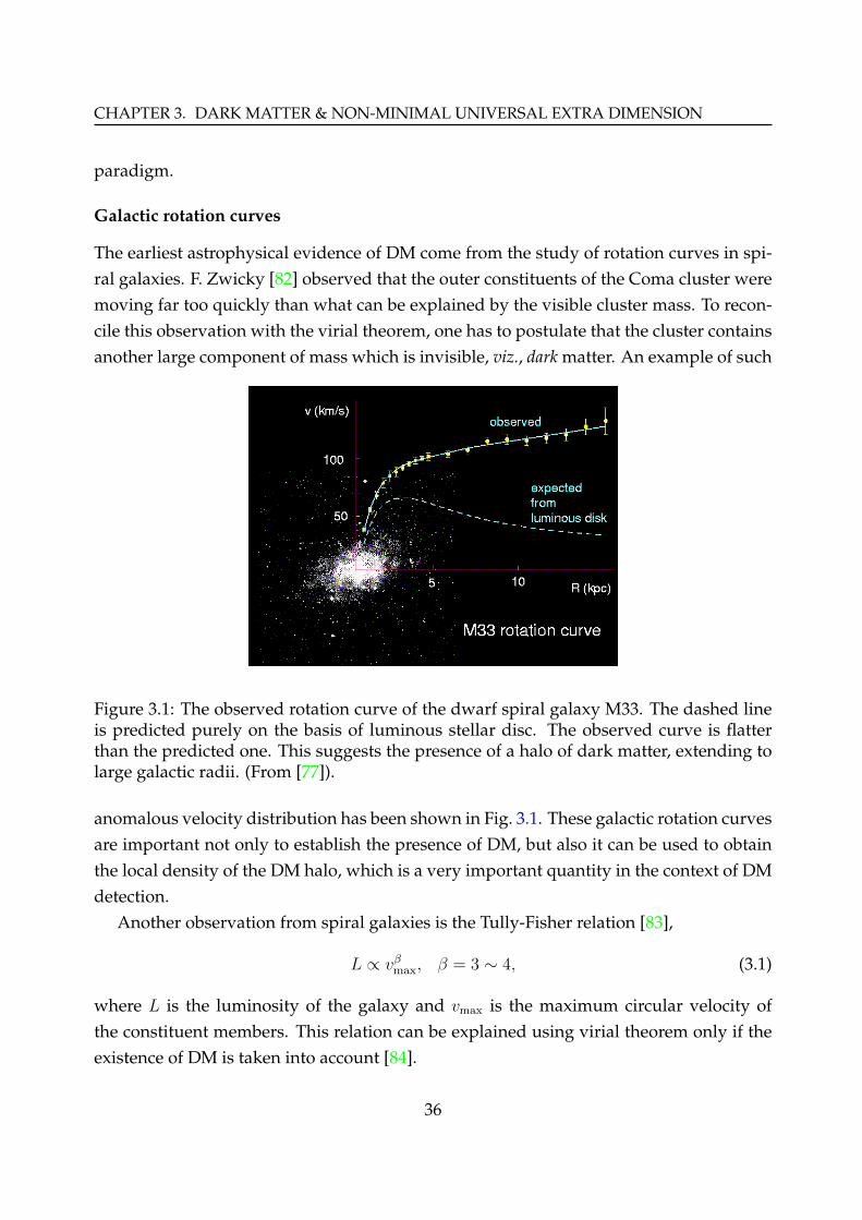
CHAPTER 3. DARK MATTER & NON-MINIMAL UNIVERSAL EXTRA DIMENSION
paradigm.
Galactic rotation curves
The earliest astrophysical evidence of DM come from the study of rotation curves in spi-ral galaxies. F. Zwicky [82] observed that the outer constituents of the Coma cluster weremoving far too quickly than what can be explained by the visible cluster mass. To recon-cile this observation with the virial theorem, one has to postulate that the cluster containsanother large component of mass which is invisible, viz., dark matter. An example of such
Figure 3.1: The observed rotation curve of the dwarf spiral galaxy M33. The dashed lineis predicted purely on the basis of luminous stellar disc. The observed curve is flatterthan the predicted one. This suggests the presence of a halo of dark matter, extending tolarge galactic radii. (From [77]).
anomalous velocity distribution has been shown in Fig. 3.1. These galactic rotation curvesare important not only to establish the presence of DM, but also it can be used to obtainthe local density of the DM halo, which is a very important quantity in the context of DMdetection.
Another observation from spiral galaxies is the Tully-Fisher relation [83],
L ∝ vβmax, β = 3 ∼ 4, (3.1)
where L is the luminosity of the galaxy and vmax is the maximum circular velocity ofthe constituent members. This relation can be explained using virial theorem only if theexistence of DM is taken into account [84].
36

3.1. DARK MATTER
Gravitational lensing and Bullet cluster
Gravitational lensing is the bending (or lensing) of light due to the presence of massiveobjects. This is a general-relativistic phenomenon. Now, galaxy clusters being very mas-sive structures show this effect. Due to this, a background object appear brighter than itotherwise would (see, e.g., [85,86]). The dark matter present in the galaxy cluster, thoughnot visible, contributes significantly to the total mass of the cluster. The best evidence todate for the existence of DM comes from the weak lensing observations of famous BulletCluster (1E0657-558), a unique cluster merger [87], where the lensing effect shows a largeamount of dark matter. On top of it, another property of DM comes out of this clustermerger, that is, the DM halos have passed right through both the gas clouds and appearalmost undisturbed after the collision. But the visible gas clouds of both clusters have un-dergone characteristic changes. It becomes evident from this, that the DM interacts withluminous matter as well as itself, very weakly.
Other astrophysical observations
There are many other observations which put the evidence of DM on a stronger footing.Big bang nucleosynthesis (BBN), in the parlance of standard big bang cosmology, allowsus to measure the primordial baryon density of the universe. On the other hand fromthe measurements of the cosmic microwave background (CMB) power spectra and large-scale structure of the universe the matter density of the universe can be obtained. Fromrecent experimental observations [74, 88] it is evident that the baryonic density and totalmatter density are different. This mandates that the DM is necessarily non-baryonic.
3.1.2 Basic properties
The existence of DM is now established almost definitely. The observations that providedoubtless evidence for the existence of DM also shed light on some of the obvious prop-erties of DM. So a theory which attempts to put forward any DM candidate must satisfythese requirements. Below we enlist some of the properties that any dark matter candi-date should abide by.
• The DM must be dark, i.e., it should have no (or extremely weak) interactions withphotons. So it must be electrically neutral. Otherwise it would be able to emit photonswhich could have modified observations from astrophysical objects, like quasars.
• The DM should have very small self-interactions.
37

CHAPTER 3. DARK MATTER & NON-MINIMAL UNIVERSAL EXTRA DIMENSION
• The interaction between DM and baryons should also be weak. Observations ofbaryonic acoustic oscillation (BAO) and CMB angular power spectrum suggest this.
• The DM must be stable. To put it another way, DM must have lifetime larger thanthe age of the universe. Actually, from the search for the decay products of DM onecan put bounds on the decay width of the DM.
• Large scale structure formation requires the DM to be "cold" enough which is al-ready non-relativistic.
• DM can not be made up of SM particles as most of them are charged. Within theambit of SM only neutrinos can be a potential DM candidate. Actually it does con-tribute in the relic density of DM minutely. But it can not be the ultimate candidatesatisfying all observations. Neutrinos are very light particles. Although its mass hasnot been measured exactly, but it is of the order of electron volt or smaller [89]. Withthis small mass it can not contribute significantly to the matter density of universe.See chapter 5 of [75] for a discussion. From the Gunn-Tremaine bound [90] we knowthat massive galactic halos can not be made up of neutrinos of mass≤ 1 MeV. More-over, being so light neutrinos are still relativistic and they constitute what is calledhot dark matter. This type of hot DM can not explain the galaxy formation rate ofthe universe after the big bang.
Thus it becomes evident that SM can not accommodate a viable DM candidate. But it isalso worth noting that although observations tend to implicate that DM is non-baryonic,there are exotic baryonic objects e.g., white dwarfs, neutron stars, super-massive blackholes which comprise MAssive Compact Halo Objects (MACHO) [91, 92], if not ruledout, are not favorable as baryonic DM candidates.
3.1.3 A few candidates
Now-a-days the most attractive, and rightfully so, non-baryonic cold dark matter candi-dates are weakly interacting massive particles (WIMP), χ. They are elementary particlesarising from many BSM theories. Normally WIMPs are heavy (∼ O(GeV-TeV)) elemen-tary particles and till now our colliders are not energetic enough to create them. But atthe time of Big Bang they were produced copiously along with a slew of other particles.In the next subsection 3.2.1 we will discuss the standard method of calculating the relicabundance of this WIMP DM.
38

3.1. DARK MATTER
For completeness, now we are going to mention a few BSM scenarios where appro-priate WIMP can arise. The list, however, is not at all exhaustive and for more detailssee e.g., [77, 93]. Any BSM theory, that tries to address DM problem, has to have a sta-ble particle in its particle spectrum. It is a general theme of these type of theories thatthey are endowed with some discrete symmetry that makes the lightest symmetry-oddparticle stable. That particle, if satisfies the relevant cosmological observational data, willbe identified as the DM candidate of that model. In the following we will discuss suchexamples.
Axion
Although its not WIMP type DM, but axion is one of the leading non-baryonic cold DMcandidates. The idea of axion, a light pseudoscalar boson, was put forward to solve thestrong CP problem [94]. A number of astrophysical observations and laboratory experi-ments put bound on axion mass to be ∼ 10−4 − 10−5eV. Even though the mass is so smallthey are still cold as their production is non-thermal. Some reviews and recent studiescan be found in [95–101].
Supersymmetry
By far the most popular and extensively studied BSM scenario is Supersymmetry (SUSY).In supersymmetric theories every SM particle has its super-partner particle differing inspin by half. In most versions of SUSY, there is a conserved discrete symmetry,R-parity, tofill up the requirement of proton stability, i.e., to avoid baryon number violating processes.It is defined as,
R = (−1)3(B−L)+2S. (3.2)
Here B and L is baryon and lepton number respectively and S is the spin of the particle.For SM particles R = 1 and for supersymmetric particles R = −1. In the minimal su-persymmetric standard model (MSSM) a linear combination of the super-partner of pho-ton, Z-boson and neutral Higgs, called neutralino is the lightest supersymmetric particle(LSP). Neutralino is of fermionic nature. This can serve as a good DM candidate. Some ofthe recent studies on neutralino LSP are [102–105]. However, there are other variants ofSUSY model where the DM candidate is not neutralino but some other supersymmetricparticle (sneutrino or gravitino for example).
39

CHAPTER 3. DARK MATTER & NON-MINIMAL UNIVERSAL EXTRA DIMENSION
Inert Higgs Doublet Model
Two Higgs doublet model (2HDM) is a simple extension of SM. In 2HDM there is oneextra Higgs doublet in addition to the SM Higgs doublet. This model is attractive becauseit is a minimal extension to SM which can accommodate additional source of CP violationwhich is needed to explain the baryon asymmetry of the universe. Also there are othermotivations. In a version of 2HDM, named as inert Higgs doublet model (IDM) [106] oneunbroken Z2 symmetry assures the stability of the lightest neutral scalar (or pseudoscalar)particle. A recent study of this DM candidate can be found in [107].
mUED and nmUED
We have already pointed out in subsection 2.1.2 that in mUED the first KK level photon,γ(1) (or effectively B(1)) is the LKP. The stability of LKP is ensured by the conservation ofKK parity. Various aspects of LKP as a dark matter has been discussed in [108–119].
In the case of nmUED the identity of LKP is no longer fixed, it can change dependingon the BLT parameter. Due to this flexibility, either of γ(1) (or B(1)), Z(1) (or W (1)
3 ), ν(1) andH(1) [66, 120] can be the DM candidate. In a later section we will study the details of theB(1) and W
(1)3 LKP case based on the results obtained in [55].
Actually there are a lot of BSM theories which predict a suitable DM particle. In theabove we just mentioned a few. We are now going to give a brief summary of the standardrelic density calculation. This will also set the notations and conventions for the latersection 3.3.2 where we will discuss the nmUED case in a detailed manner.
3.2 Relic density
3.2.1 Standard calculation of relic density
A brief history of WIMPs is as follows. After its production such particles remain in ther-mal equilibrium and in abundance when the temperature of the universe is greater thanthe mass of the particle, mχ. The equilibrium abundance (or density) of these particlesis maintained by the annihilation of these particles with their anti-particles, χ into otherlighter particles (X), (χχ→ XX) and vice versa, (XX → χχ). But the temperature of theuniverse decreases and when it becomes less than mχ, the equilibrium abundance drops.Clearly the annihilation (χχ → XX) rate will also drop. At the point when the annihila-tion rate falls below the expansion rate of the universe, H , the interactions maintaining
40

3.2. RELIC DENSITY
the thermal equilibrium "freeze out". Since the χs are stable (i.e., they can not decay) thenafter the freeze out the abundance of them also become fixed and what remains afterwardis just the thermal relic of WIMPs. In the following we will describe how to calculate therelic density following standard equilibrium thermodynamics [75].
It is a fairly good approximation that the early universe was in thermal equilibrium.The number density of the particle, χ, in thermal equilibrium is given by,
neq =g
(2π)3
∫d3pf(~p), (3.3)
where g is the internal degrees of freedom (DoF) of χ and f(~p) is the phase space distribu-tion function and is given by usual Fermi-Dirac (FD) or Bose-Einstein (BE) distribution,
f(~p) =1
exp(E−µT
)± 1
, (3.4)
where ’+’ is for FD statistics and ’-’ for BE statistics and µ is the chemical potential of thecorresponding species.In the relativistic limit (T m) and T µ,
neq =
(ζ(3)π2
)gT 3 for BE statistics,(
3ζ(3)4π2
)gT 3 for FD statistics,
(3.5)
and in the non-relativistic limit (m T ), both for FD and BE species,
neq = g
(mT
2π
)3/2
exp
(m− µT
). (3.6)
The evolution, with time (or temperature), of the number density of χ is given by theBoltzmann equation,
dn
dt= −3Hn− 〈σv〉(n2 − n2
eq), (3.7)
whereH =
1
a
da
dt(3.8)
is the Hubble parameter (a is the scale factor of the universe) and 〈σv〉 is the thermallyaveraged annihilation cross section times relative velocity. The first term in the right-hand side of Eq. 3.7 accounts for the reduction of number density due to the expansionof the universe. The second term takes care of decrease (or increase) in n due to theinteraction of χwith other particles in the spectrum. After solving Eq. 3.7 we can calculatethe contribution of χ in the energy density of the universe by defining the quantity, Ωχ as,
Ωχh2 ≡ ρχ
ρc=mχn
ρc, (3.9)
41
CHAPTER 3. DARK MATTER & NON-MINIMAL UNIVERSAL EXTRA DIMENSION
where h is the Hubble parameter in the units of 100 km s−1 Mpc−1 and ρc is the criticaldensity of the universe and is given by,
ρc =3H2
8πGN
. (3.10)
At the point when the annihilation rate Γ = n〈σv〉 . H , the annihilation of χs ceases andthe relic abundance remains fixed afterward. At the freeze out temperature the annihila-tion cross section can be expanded in powers of squared relative velocity,
σv = a+ bv2 + . . . , (3.11)
where the first term comes from the s-wave annihilation and the second from both s andp-wave annihilation. A nice discussion on the these type annihilation cross section in thelow velocity limit can be found in [121]. In most of the cases these first two terms in theexpansion are enough to produce a fair estimate of the relic density. With appropriateapproximations Eq. 3.7 can be solved analytically and the relic density is given by [75,108, 110, 122],
Ωχh2 ≈ 1.04× 10⁹/1GeV
MPl
xF√g∗(xF )
1
a+ 3bxF
, (3.12)
where MPl is the Planck mass and g∗(xF ) is the total number of relativistic DoF at thefreeze out temperature. Here xF (= m/TF , TF being the freeze out temperature) is solvedfrom the equation,
xF = ln
(15
8
√5
2
g
2π3
mMPl(a+ 6b/xF )√g∗(xF )xF
). (3.13)
However, there are three important exceptions to the validity of the above mentionedprescription1 [76, 123],
• annihilation near mass thresholds (i.e., kinematically forbidden channels at T = 0,but can be significant at higher temperatures),
• coannihilations (i.e., when there are particles which are slightly heavier than χ andaffect the number density of χ), and
• resonances in the annihilation cross section (i.e., when the mχ is half the mass of theparticle exchanged in the s-channel annihilation process).
Systematic treatment of finite temperature corrections takes care of the first case. Butthis marginally affects the relic density. The latter two cases depend significantly on theparticle spectrum and thus on the parameters of the theory.
1In the relevant parameter space of mUED or nmUED, only coannihilation will play an important role.
42

3.2. RELIC DENSITY
3.2.2 Coannihilation
In the particle spectrum of the theory if there are particles nearly degenerate with the relicparticle then the freeze out of these particles occurs almost at the same epoch when therelic particle χ decouples and can affect the relic abundance of χ. For example, considerthere are N particle species, χi (i = 1, 2, . . . , N) and mi < mj if i < j, i.e., χ1 is the light-est particle. The number density ni of each species χi will obey appropriate Boltzmannequations. Moreover, all the heavier particles (χi with i > 1) will ultimately decay to χ1.So from any number Ni of χi particles we end up getting exactly Ni number of χ1 at theend of the decay chain. Thus to determine the relic abundance of χ1 it is meaningful tostudy the evolution of the number density n(=
∑j nj) instead of each number density
separately. The Boltzmann equation will be modified from the form we have given inEq. 3.7 as,
dn
dt= −3Hn− 〈σeffv〉(n2 − n2
eq). (3.14)
The quantity σeff is given by,
σeff(x) =1
g2eff
N∑
i,j=1
σijFiFj (3.15)
where
geff(x) =N∑
i=1
Fi(x), (3.16a)
Fi(x) = gi(1 + ∆i)3/2 exp(−x∆i), (3.16b)
with∆i =
mi −m1
m1
and x =m
T. (3.17)
Here σij ≡ σ(χiχj → SM) and gi is the number of internal DoF of the species χi takingpart in the annihilation or coannihilation process. In the non-relativistic limit we have,〈σeffv〉 ∼ aeff(x) + beff(x)v2 +O(v4). The approximate expression for the relic density willnow become,
Ωχh2 ≈ 1.04× 10⁹/1GeV
MPl
xF√g∗(xF )
1
Ia + 3IbxF
, (3.18)
where Ia,b are given by,
Ia = xF
∫ ∞
xF
aeff(x)x−2dx, (3.19a)
43

CHAPTER 3. DARK MATTER & NON-MINIMAL UNIVERSAL EXTRA DIMENSION
Ib = 2x2F
∫ ∞
xF
beff(x)x−3dx. (3.19b)
The freeze out temperature is given by,
xF = ln
(15
8
√5
2
geff(xF )
2π3
m1MPl(aeff(xF ) + 6beff(xF )/xF )√g∗(xF )xF
). (3.20)
After this discussion on relic density calculation we are now in a position to look atmUED and nmUED in the light of dark matter observations.
3.3 Relic density in mUED and nmUED
In this section we will discuss the relic density constraints on mUED and nmUED. Ashas been already mentioned earlier, in mUED, B(1) is the dark matter candidate and innmUED the identity of DM is not fixed. We will first see in the case of mUED, ifB(1) is theLKP then how it satisfies the relic density observation, i.e., how do the observations putconstraint on the parameters of mUED. In the later part we will see how those constraintscan be relaxed if we consider the nmUED. We will also discuss how well-suited otherpossible candidates in nmUED are.
3.3.1 mUED
In the context of mUED, we know that the LKP is the first KK level photon, γ(1) whichdue to a small mixing angle behaves purely like the first KK level U(1)Y gauge bosonB(1). After radiative correction its mass gets the smallest correction and it remains theLKP. Even in mUED departing from the standard scenario if one by hand relaxes the re-striction that fields which experience only the U(1)Y interaction are lighter than those ofthe fields which experience the SU(2) interaction, then W
(1)3 (i.e., first KK level Z-boson)
or level one KK neutrino ν(1) can be considered as the LKP [108, 109]. As it stands, ν(1) isruled out as an LKP from DM direct detection experiments [109]. Another less popularcandidate for LKP is first level KK graviton. The problem is that since KK graviton willhave very feeble gravitational interaction only, their inefficient annihilation will lead tooverclosure of the universe. Also there are other stringent constraints on KK gravitonas the LKP [124]. Another possibility is to add extra fields, e.g., right handed neutrinos,in the already existing spectrum. Such possibilities and their advantages have been dis-cussed in [125–127]. Below we will present the case of γ(1) (or B(1)) and Z(1) (or W (1)
3 ) LKPfollowing [108, 110, 117].
44

3.3. RELIC DENSITY IN MUED AND NMUED
Actually these are variants of mUED model where the mass spectra is not kept as it isobtained after radiative corrections and the usual practice is to take a different LKP (ν(1)
or Z(1) or H(1)2), purely from phenomenological point of view, and study their effects.Not only the identity of LKP but also the mass splitting (e.g., ∆q1 in [117]) is put in byhand.
In the case of B(1) LKP, the relevant cross sections are the annihilation of B(1) pairsinto fermions and into Higgs boson. If the EWSB effects are neglected then there are nochannels into vector bosons. If the coannihilation processes are neglected then from theobserved value of relic density the allowed mass for B(1) lies in the range 900− 1200 GeV.With coannihilation effects taken into account this bound decreases. Considering onlythe coannihilation of first level singlet electron e
(1)R with B(1), the allowed band of mB(1)
becomes 600 − 1050 GeV [108], depending on the mass splitting ∆e(1)R
. A more elaboratestudy, done in [110], with a modified data set and taking coannihilation processes forother set of particles as well, reveals that the allowed range of mB(1) should be 500 − 600
GeV which is in good agreement with an independent study done in [114]. In a similarstudy [117] on a variant of mUED model with B(1) LKP it is shown (left panel of Fig. 3.2)that allowed rangemB(1) (presented asmγ1 in the figure) is from 500−1600 GeV dependingon the mass splitting of B(1) with q(1).
The case of Z(1) (or W (1)3 ) LKP in the context of a variant of mUED3 has been discussed
in [117]. Due to the larger value of weak gauge coupling the annihilation cross section ofZ(1) is relatively large. The relic density as a function of Z(1) mass, mZ(1) has been shownin Fig. 3.2 (right panel). It is evident from this figure that quark coannihilation processesincrease the effective cross section reducing the relic density and thus the allowed bandof mZ(1) consistent with data becomes 1800 − 2700 GeV depending on the mass splittingwith first KK level quarks which in this case are the next to lightest LKPs (NLKP). We willsee a similar effect in the case of nmUED too.
It is worth mentioning that the inclusion of second KK level particles, in the calcula-tion, changes many of the bounds mentioned earlier. Actually the second level particlescan be exchanged in an s-channel annihilation of two level one particles. For example, inB(1)B(1) annihilation, second level HiggsH(2) can be exchanged in s-channel. So there is apossibility of enhancement in annihilation cross section near resonance. Due to this, thereis significant reduction in relic abundance [111, 112, 116]. The second level particles canaffect the relic density not only through s-channel resonance but also they can be singly
2See e.g., [128] for H(1) LKP study.3For a different discussion of Z(1) LKP see, for example, [129]
45

CHAPTER 3. DARK MATTER & NON-MINIMAL UNIVERSAL EXTRA DIMENSION
Figure 3.2: Relic density of LKP (i) γ(1) (left) and (ii) Z(1) (right) as a function of LKPmass. The green band gives 2σ allowed region from WMAP 5yr data [130], ΩCDMh
2 ∈(0.1037, 0.1161) and the vertical cyan band excludes the mass of LKP from precision data.Here KK singlet and doublet quarks are assumed to be degenerate and the mass of thelevel one quarks are varied by hand, such that ∆q1 = 0.01, 0.02, 0.05, 0.1 and 0.5. AlsoZ(1) and W (1)± are taken to be degenerate. The red dotted line gives the result of fullmUED calculation including all coannihilation processes. Adapted from [117].
produced in association with SM particle in the final state and subsequently this leveltwo particle decays to SM particles through loop induced processes. In such a scenariocoannihilation processes can even dominate over the annihilation processes which in turnreduce the relic density. Considering these points, in a recent study [118], it is pointed outthat the preferred compactification scale (1/R) and thus the mass of the LKP should be1.3 TeV. However in non-minimal version of UED the LKP can have masses much lowerthan this bound while satisfying other constraints.
3.3.2 nmUED
We are now going to discuss the nmUED scenario. We have described the model inSec. 2.2. The action is given in Eqs. 2.8. We have already mentioned that in nmUED themass spectrum and couplings are dependent on the BLT parameters (rX for the field X).We will use the dimensionless parameter RX(= rX/R), where R is the compactificationradius. We will concentrate on the bosonic LKP states:4, B(1) and W
(1)3 . The discussion of
this subsection will follow [55].
4Depending on the BLT parameter ν(1) or H(1) can also be LKP.
46

3.3. RELIC DENSITY IN MUED AND NMUED
From our earlier discussion it is evident that M(1)(= m1R) is determined entirely bythe BLT parameter, RBLT, and the compactification radius R. The gauge coupling playsno role. Therefore the earlier discussion applies for both W
(1)3 and B(1) as long as the
appropriate BLT parameters are used. Which of them will be identified as LKP is deter-mined purely by the choice of the respective BLT parameters. In the subsequent part ofthis subsection we investigate the prospects of these WIMPs playing the role of the darkmatter particle.
On the electroweak gauge boson mass matrix
Before going to the details of DM study it is important to clarify some of the points re-garding the masses of B(1) and W
(1)3 . It is imperative to see how the inclusion of zero
mode masses (which we did not discuss in the subsection 2.2.1) affect the masses andmixing of W (1)
3 and B(1). In a 5D theory the electroweak gauge boson eigenstates withBLKT have been discussed in the literature [66]. It can be easily verified that for the rangeof BLKT parameters which we will consider the states of different KK level, n, mix neg-ligibly. Further, only if the BLKT parameters for the B and W gauge bosons are exactlyequal (or their difference is very small) the mixing between B(1) and W (1)
3 is substantial, itbeing equal to the zero-mode weak mixing angle in the case of equality. If (rB − rW )/R isof order 0.1 (or larger) this mixing is negligible. This can be verified from the mass matrixwhich we now discuss.
The mass matrix for the n = 1 neutral electroweak gauge bosons including spon-taneous electroweak symmetry breaking, as well as the extra-dimensional contribution(discussed in Sec. 2.2) is5:
MW
(1)3 B(1) =
g22v2
4SWSHIW3W3 +m2
W(1)3
−g2g1v2
4
√SWSBSH
IW3B
−g2g1v2
4
√SWSBSH
IW3Bg21v
2
4SBSHIBB +m2
B(1) ,
(3.21)
where
Iij =
∫ πR
0
(1 + rHδ(y) + δ(y − πR)) a(1)i (y)a
(1)j (y)dy, (i, j = W3, B). (3.22)
Above, rH is the strength of the Higgs scalar BLKT and RH = rH/R. Also,
a(1)W3
(y) = N(1)W3
[cos(mW
(1)3y)−rWmW
(1)3
2sin(mW
(1)3y)]
, (3.23a)
5Here mW
(1)3
and mB(1) stand for the extra-dimensional mass contribution m1, obtained from solvingthe mass determining transcendental equation, for the n = 1, W3 and B states, respectively.
47

CHAPTER 3. DARK MATTER & NON-MINIMAL UNIVERSAL EXTRA DIMENSION
a(1)B (y) = N
(1)B
[cos (mB(1) y)− rBmB(1)
2sin (mB(1) y)
], (3.23b)
with N(1)W3
, N (1)B being normalization factors as in Eq. 2.20. The 5D gauge couplings g2, g1
and the vacuum expectation value (vev) v are related to the 4D couplings g2, g1 respec-tively and the vev v through
g2 = g2
√πR SW , g1 = g1
√πR SB , v = v/
√πR SH , (3.24)
where
SW =
(1 +
RW
π
), SB =
(1 +
RB
π
), SH =
(1 +
RH
π
). (3.25)
A few comments about the mass matrix, MW
(1)3 B(1) in Eq. 3.21 are in order. The ma-
trix is given in the W (1)3 − B(1) basis6. As an estimate of the relative magnitudes of the
terms inMW
(1)3 B(1) , notice that the Si are O(1) as are the overlap integrals Iij . Hence the
contributions to the mass matrix from the EWSB are O(v2). The extra-dimensional con-tributions, m2
(W3/B)(1), are of the order of (1/R)2 and are always dominant by far. As a
consequence these terms affect significantly the mass eigenvalues and the mixing is neg-ligible for (RW − RB) ∼ 0.1 or larger7. So, in our discussion below we take B(1) and W
(1)3
to be the neutral electroweak gauge eigenstates. This is similar to the case in mUED. Thecontributions to the masses from the EWSB are insignificant and hence dropped. It isverified that for the cases of our interest there is negligible dependence of the results onthe Higgs BLKT strength, rH . In our calculations we keep RH = 0.1 throughout.
Dark matter study
Since in nmUED masses of the KK-excitations are determined by the BLT parameters, itis the choice of these BLT parameters which determine whether or not the mass of anyKK-excitation would lie close to the relic particle mass (∆i ≤ 10%) so that their coanni-hilation process could contribute significantly. In our analysis we have chosen the BLKTparameters for quarks, gluons and right-handed leptons such that their masses are suffi-ciently larger than the B(1) mass and their contributions to coannihilation are negligible.With this choice the only relevant coannihilation processes are those of KK-excitations ofthe left-handed lepton doublets.
6It can be easily checked that the mixing with states of n 6= 1 is very small.7If RW = RB then the dominant diagonal terms become equal and keep the mixing unaffected and
simply make a constant shift in the masses of the eigenstates. In this case the mixing between W(1)3 and
B(1) is just like the Standard Model with tan θ = g1/g2.
48

3.3. RELIC DENSITY IN MUED AND NMUED
B(1) annihilation B(1)-lepton scattering
B(1)B(1) → ff ν(1)L B(1) → W+`−
B(1)B(1) → h+h− ν(1)L B(1) → W−`+
ν(1)L B(1) → Zν`
ν(1)L B(1) → Zν`
`(1)−L B(1) → W−ν`
`(1)+L B(1) → W+ν`
`(1)−L B(1) → Z`−
`(1)+L B(1) → W+ν`
Table 3.1: The B(1) annihilation and relevant B(1)-lepton scattering process that are im-portant for the relic density calculation of B(1).
In Tables 3.1-3.3 the relevant processes which are used to calculate effective cross sec-tion, σeff , have been listed. Some of the couplings between the level one KK particles andSM particles will get modification in nmUED in view of non-trivial mode functions ofthe KK excitations8. Consequently, the cross sections of some of the processes which arecontributing in σeff will accordingly be scaled up or down with respect to their mUEDvalues.
ν(1) annihilation and scattering `(1) annihilation and scattering
ν(1)L ν
(1)L → ff `
(1)+L `
(1)−L → h+h−
ν(1)L ν
(1)L → h+h− `
(1)+L `
(1)−L → ZZ, Zγ, γγ
ν(1)L ν
(1)L → ZZ `
(1)+L `
(1)−L → W+W−
ν(1)L ν
(1)L → W+W− `
(1)±L `
(1)±L → `±`±
ν(1)L ν
(1)L → ν`ν` `
(1)±L `
′(1)±L → `±`′±
ν(1)L ν
′(1)L → ν`ν
′` `
(1)±L `
′(1)∓L → `±`′∓
ν(1)L ν
′(1)L → ν`ν`′ `
(1)+L `
′(1)−L → ff or `+
R`−R
ν(1)L ν
′(1)L → `−`′+ `
(1)+L `
′(1)−L → ν`ν` or `+
L`−L
ν(1)L ν
(1)L → `+`− `
(1)+L `
′(1)−L → ν`ν`′
Table 3.2: The ν(1) and `(1) annihilation and scattering processes which contribute to therelic density calculation.
8Such interactions with the Feynman rules are listed in the Appendix at the end of this chapter.
49
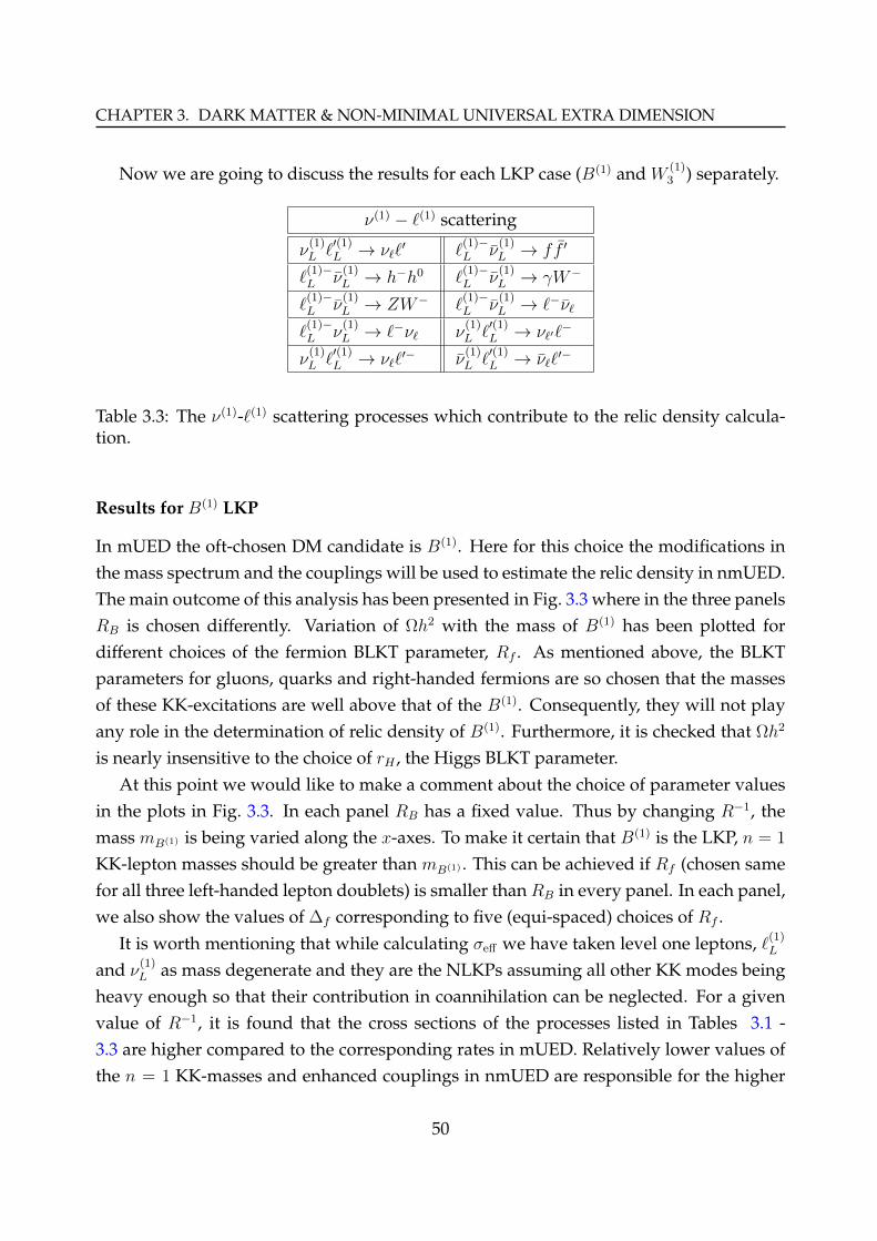
CHAPTER 3. DARK MATTER & NON-MINIMAL UNIVERSAL EXTRA DIMENSION
Now we are going to discuss the results for each LKP case (B(1) and W(1)3 ) separately.
ν(1) − `(1) scattering
ν(1)L `
′(1)L → ν``
′ `(1)−L ν
(1)L → ff ′
`(1)−L ν
(1)L → h−h0 `
(1)−L ν
(1)L → γW−
`(1)−L ν
(1)L → ZW− `
(1)−L ν
(1)L → `−ν`
`(1)−L ν
(1)L → `−ν` ν
(1)L `
′(1)L → ν`′`
−
ν(1)L `
′(1)L → ν``
′− ν(1)L `
′(1)L → ν``
′−
Table 3.3: The ν(1)-`(1) scattering processes which contribute to the relic density calcula-tion.
Results for B(1) LKP
In mUED the oft-chosen DM candidate is B(1). Here for this choice the modifications inthe mass spectrum and the couplings will be used to estimate the relic density in nmUED.The main outcome of this analysis has been presented in Fig. 3.3 where in the three panelsRB is chosen differently. Variation of Ωh2 with the mass of B(1) has been plotted fordifferent choices of the fermion BLKT parameter, Rf . As mentioned above, the BLKTparameters for gluons, quarks and right-handed fermions are so chosen that the massesof these KK-excitations are well above that of the B(1). Consequently, they will not playany role in the determination of relic density of B(1). Furthermore, it is checked that Ωh2
is nearly insensitive to the choice of rH , the Higgs BLKT parameter.At this point we would like to make a comment about the choice of parameter values
in the plots in Fig. 3.3. In each panel RB has a fixed value. Thus by changing R−1, themass mB(1) is being varied along the x-axes. To make it certain that B(1) is the LKP, n = 1
KK-lepton masses should be greater than mB(1) . This can be achieved if Rf (chosen samefor all three left-handed lepton doublets) is smaller thanRB in every panel. In each panel,we also show the values of ∆f corresponding to five (equi-spaced) choices of Rf .
It is worth mentioning that while calculating σeff we have taken level one leptons, `(1)L
and ν(1)L as mass degenerate and they are the NLKPs assuming all other KK modes being
heavy enough so that their contribution in coannihilation can be neglected. For a givenvalue of R−1, it is found that the cross sections of the processes listed in Tables 3.1 -3.3 are higher compared to the corresponding rates in mUED. Relatively lower values ofthe n = 1 KK-masses and enhanced couplings in nmUED are responsible for the higher
50

3.3. RELIC DENSITY IN MUED AND NMUED
Figure 3.3: Variation of Ωh2 with relic particle mass, mB(1) . Curves for different choicesof the fermion BLKT parameter Rf are shown and the corresponding ∆f indicated. Thenarrow horizontal blue band corresponds to the 1σ allowed range of relic particle densityfrom Planck data [74]. The allowed 1/R (or mB(1)) can be read off from the intersectionsof the curves with the allowed band. The three panels are for different choices of RB, theBLKT parameter for B.
reaction rates for a given value of R−1. Thus the numerical value of the relic density innmUED is always less than in mUED as long as the BLKT parameters are positive (asused in our analysis).
It is possibly useful to mention here the magnitudes of the coefficients Ia and Ib inEq. 3.18 which reflect the model dynamics. For the choices that we have made for RB andRf , Ia and Ib are in the range of (1− 10) pb. Both Ia and Ib decrease with increasing mB(1) .
One can see from Fig. 3.3 that Ωh2 increases with increase of R−1 or RB. Both increasesserve to reduce mB(1) and also enhance the couplings. In contrast, Ωh2 decreases withincreasing Rf , the fermion BLKT coefficient. Unlike in mUED, the allowed range of R−1
depends on Rf in nmUED. This is expected, as Rf moves away from RB the splitting inmass between B(1) and fermions, ∆f , increases (noted in the figures) and coannihilationbecomes less important.
It is seen from Fig. 3.3 that depending on the choice of RB and Rf the allowed rangeof R−1 can be as much as 0.6 TeV to 2 TeV or even more, while remaining consistent withthe observed dark matter limits. It should be kept in mind that in nmUED the mass of theLKP is actually a little lower than R−1 as seen in the lower x-axes in the panels and alsoillustrated in Fig. 2.3.
In passing we would like to comment on the upper bounds on R−1 that arise by de-manding that the LKP does not overclose the universe. This can happen if Ωh2 ≈ 0.48.Some sample results are presented in Table 3.4. To be conservative, the smallest Rf hasbeen chosen for every RB (which implies the largest ∆f ) in Fig. 3.3. For larger Rf the
51
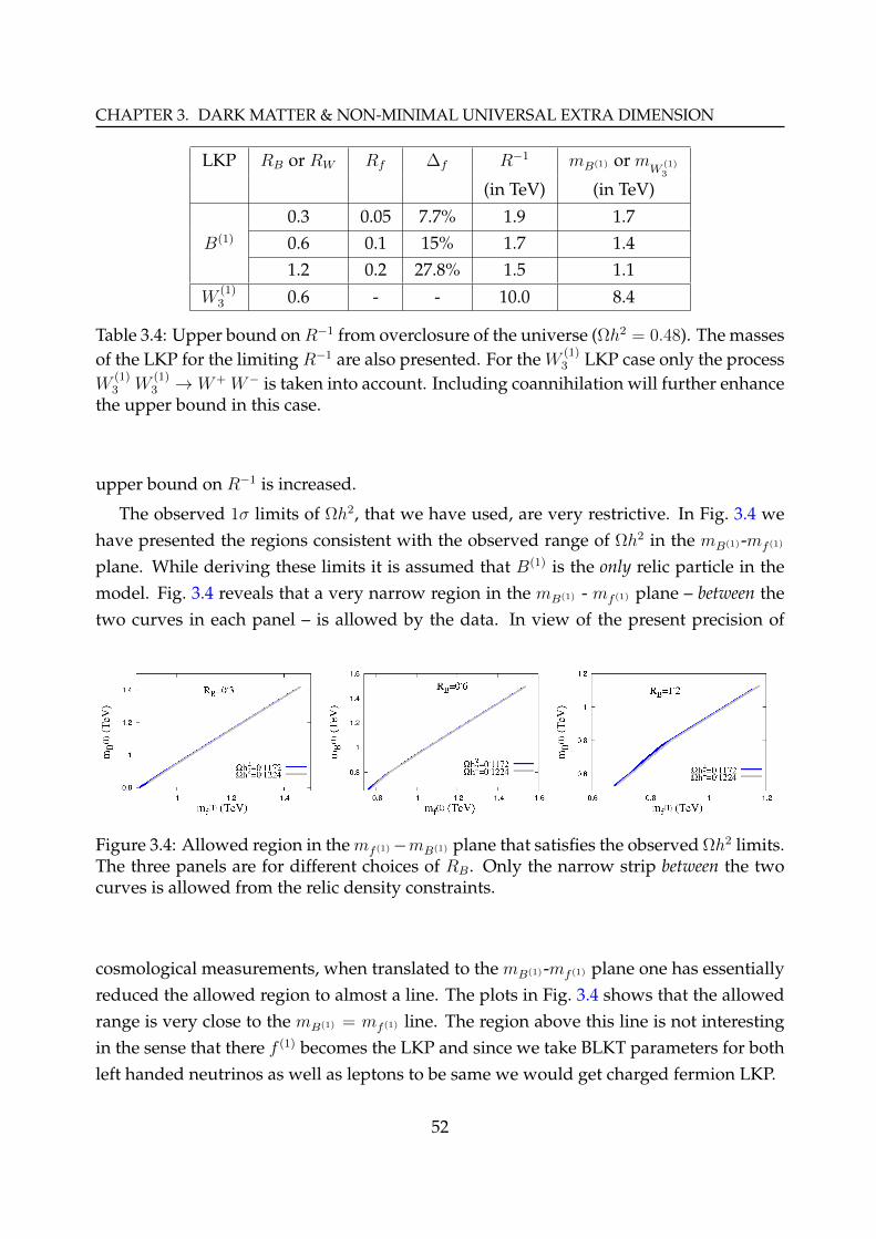
CHAPTER 3. DARK MATTER & NON-MINIMAL UNIVERSAL EXTRA DIMENSION
LKP RB or RW Rf ∆f R−1 mB(1) or mW
(1)3
(in TeV) (in TeV)
0.3 0.05 7.7% 1.9 1.7B(1) 0.6 0.1 15% 1.7 1.4
1.2 0.2 27.8% 1.5 1.1
W(1)3 0.6 - - 10.0 8.4
Table 3.4: Upper bound onR−1 from overclosure of the universe (Ωh2 = 0.48). The massesof the LKP for the limiting R−1 are also presented. For the W (1)
3 LKP case only the processW
(1)3 W
(1)3 → W+ W− is taken into account. Including coannihilation will further enhance
the upper bound in this case.
upper bound on R−1 is increased.
The observed 1σ limits of Ωh2, that we have used, are very restrictive. In Fig. 3.4 wehave presented the regions consistent with the observed range of Ωh2 in the mB(1)-mf (1)
plane. While deriving these limits it is assumed that B(1) is the only relic particle in themodel. Fig. 3.4 reveals that a very narrow region in the mB(1) - mf (1) plane – between thetwo curves in each panel – is allowed by the data. In view of the present precision of
Figure 3.4: Allowed region in themf (1)−mB(1) plane that satisfies the observed Ωh2 limits.The three panels are for different choices of RB. Only the narrow strip between the twocurves is allowed from the relic density constraints.
cosmological measurements, when translated to the mB(1)-mf (1) plane one has essentiallyreduced the allowed region to almost a line. The plots in Fig. 3.4 shows that the allowedrange is very close to the mB(1) = mf (1) line. The region above this line is not interestingin the sense that there f (1) becomes the LKP and since we take BLKT parameters for bothleft handed neutrinos as well as leptons to be same we would get charged fermion LKP.
52

3.4. DIRECT DARK MATTER DETECTION IN MUED AND NMUED
Results for W (1)3 LKP
The masses of the n > 0 KK-states are determined by their respective BLKT parameters rior equivalently Ri = ri/R. Thus to avoid a fermion LKP one must choose RB, RW > Rf .Besides the just discussed case of RB > RW , corresponding to B(1) LKP, one shouldalso consider RW > RB which makes W (1)
3 the dark matter candidate9. In such a caseit is found that the annihilation cross section is large (notably because of the processW
(1)3 W
(1)3 → W+W−) and therefore the relic density is too small10. The relic density as
Figure 3.5: Variation of the relic density with mW
(1)3
in the case of W (1)3 LKP. The current
observed value (∼ 0.12) disfavors this alternative.
a function of the W (1)3 mass, m
W(1)3
is shown in Fig. 3.5 for a typical value of RW = 0.6.It is important to note that the obtained relic density is far below the observed [74] value(around 0.12). For RW = 0.6 the lower (upper) bounds on Ωh2 – which are outside therange of the figure – correspond to R−1 = 4.66 (4.7) TeV with the respective W (1)
3 masses3.92 (4.04) TeV. This establishes that W (1)
3 would not be an attractive dark matter candi-date for easy detection at the LHC unless the DM consists of several components andW
(1)3 is one of them11.
3.4 Direct Dark Matter Detection in mUED and nmUED
Once the evidence of dark matter has been proved with certainty from various observa-tions, the next exigent issue in the DM paradigm is to detect it and pinpoint its othercharacteristic features. Presently various DM search strategies are operative e.g., collider
9For a different discussion of the W (1)3 LKP see, for example, [129].
10The coannihilation in this case has not been considered as it would further reduce the relic density.11The overclosure bound on R−1 for RW = 0.6 is 10 TeV (see Table 3.4).
53

CHAPTER 3. DARK MATTER & NON-MINIMAL UNIVERSAL EXTRA DIMENSION
searches, indirect searches (searching for annihilation products of DM which have fea-tures allowing for a discrimination from other astrophysical background sources) anddirect searches (scattering of DM particles off ordinary matter). We will begin this sectionwith a brief exposition to the direct detection methods of WIMPs. Then in the later partsits implications on mUED and nmUED will be examined. Actually from Fig. 3.6 it is ev-
Figure 3.6: Schematic presentation of DM interaction (taken from [131]).
ident that the amplitude for DM annihilation to SM particles is related to the amplitudefor elastic scattering of DM particles from SM particles by crossing symmetry. Thus it isexpected that the DM will have small, but non-zero coupling to atomic nuclei throughthe coupling to quarks. Now, assuming a certain DM distribution in our galaxy, such ex-periments can be devised where DM particle scatters off a target nucleus and releases anamount of energy which will be measured as the recoil of the target nucleus or ionizationof the target medium12.
The calculation of DM-nuclei interaction proceeds through three important steps. Thefirst step involves the calculation of interactions of DM with quarks and gluons. Al-though straightforward, this procedure is marred with model parameter uncertainties asthese creep in at various stages of the calculations. In the second step these microscopicinteractions are to be translated to the interactions of DM with nucleons. To perform thisone needs the matrix elements of quark and gluon operators in a nucleon state. At thiscomes in uncertainty stemmed from nuclear physics. The last step requires adding up theDM-nucleon interactions to obtain the DM-nucleus interactions by using nuclear wave
12See, for example [132] for an overview of various experimental setups.
54

3.4. DIRECT DARK MATTER DETECTION IN MUED AND NMUED
functions. Various nuclear form factors are to be used in this step, leaving scope of morenuclear physics uncertainty13. One important aspect of this calculation is that the scatter-ing of DM happens in extreme non-relativistic limit. It is straightforward to show that inthis limit the axial vector current leads to interaction between quark spin and DM parti-cle spin, also vector and tensor currents take the form of scalar interactions. Thus thereare two types of interactions that the DM-nucleus elastic scattering proceeds through,namely, spin independent or scalar interactions and spin dependent interactions. In thespin independent interaction the mass of nucleus plays the major role whereas for thecase of spin dependent interaction it is the spin of the nucleus [134]. It may so happenthat a specific DM candidate (e.g., neutralino in the case of SUSY or B(1) in the case ofmUED or nmUED) has both scalar as well as spin dependent interactions. In that case thefull elastic scattering cross section is the sum of these two interactions.
There are many experiments, operative presently (and in the past), which are tryingto search DM by direct detection method. They fall into different classes dependingon the detection technique and detector material, for example cryogenic crystal experi-ments (e.g., CDMS [135], EDELWEISS [136], CRESST [137]), scintillator experiments (e.g.,DAMA [138]), noble liquid experiments (e.g., XENON [139, 140], LUX [141]) etc. In ourstudy of nmUED (subsection 3.4.2, following [55]) we will compare our results with theXENON experiment. Before going to nmUED it will not be out of place to mention a fewthings about the direct detection studies in the context of mUED.
3.4.1 mUED
In mUED the detection prospect of B(1) LKP has been discussed in [142] followed bysubsequent studies in [109,117]. In [142], taking B(1) to be the LKP it has been shown thatthe scalar cross sections are suppressed with respect to the spin dependent one. As wewill see in the next subsection this is the case for nmUED too.
In Fig. 3.7 it is illustrated that the cross sections can be increased up to one order de-pending on the mass splitting ∆q(1) which has been varied by hand. The cross sections arebelow the reach of currently running experiments. Experiments with improved sensitiv-ity will be required to probe the scenario.
In a variant of mUED, the first level KK neutrino, ν(1) is also considered to be theLKP [109]. But it has been shown that this case is not viable as to be consistent with theobservations of experiments like, EDELWEISS [143] or CDMS [144] the ν(1) LKP should
13For a nice pedagogic review on direct detection see, e.g., [133]
55

CHAPTER 3. DARK MATTER & NON-MINIMAL UNIVERSAL EXTRA DIMENSION
10-7
10-6
10-5
0.6 0.7 0.8 0.9 1 1.1 1.2
∆ = 15%
∆ = 10%∆ = 5%
mB
(1) (TeV)
σsp
in(B
(1) n
→ B
(1) n
) (p
b)
10-10
10-9
0.6 0.7 0.8 0.9 1 1.1 1.2
∆ = 15%
∆ = 10%
∆ = 5%
mB
(1) (TeV)
σS(B
(1) n
→ B
(1) n
) (p
b)
Figure 3.7: Spin dependent and scalar LKP-nucleon cross section as a function of B(1)
mass for ∆q(1) = 5, 10, 15% and mH = 120 GeV. Adapted from [109].
have a mass & 50 TeV. But relic density calculations do not favor the ν(1) masses to begreater than 10 TeV. The direct detection study of the W (1)
3 (or Z(1)) LKP has been per-formed in [117, 145].
3.4.2 nmUED
In this subsection we will consider nmUED and how the DM direct detection experimentsconstrain it. At this point it would be useful to recall that the main difference with themUED scenario will come through the BLKT parameters which modify the mass spectraas well as couplings. The discussion of this subsection will closely follow [55].
We would like to elaborate on the prospects of direct detection ofB(1) at an experimentsuch as XENON [140, 146]. The actual event rates at such an experiment will not be esti-mated; instead, we will present the spin dependent and spin independent cross sectionsof B(1) scattering off Xenon nuclei (A = 131, Z = 54). Event rates and cross sections ofDM in the context of mUED have been obtained in ref. [109, 142]. As masses and also thecouplings in nmUED show a distinctive departure from the corresponding quantities inUED, we wish to revisit the calculation.
We have already mentioned that the scattering cross section of dark matter off nucleiis ultimately related to its scattering from quarks. Also in the non-relativistic limit thetotal cross section can have two components: the spin-independent (i.e., scalar) and spin-
56

3.4. DIRECT DARK MATTER DETECTION IN MUED AND NMUED
dependent parts.The spin independent part of the scattering cross section ofB(1) with a nucleus of mass
mN with atomic number Z and mass number A at zero momentum transfer is given by,
σscalar0 =
m2N
4π(mB(1) +mN)2
(ZfB
(1)
p + (A− Z)fB(1)
n
)2
, (3.26)
wherefB
(1)
p,n = mp,n
∑
q
γq + βqmq
f(p,n)Tq
. (3.27)
The subscript p and n refers to the proton and neutron respectively. In our numericalcalculations we have used f
(p,n)Tq
= 〈qq〉p,n(mq/mp,n), that relate the quark-level cross sec-tions to that for the nucleons, as given in [76]. The model dependence of the specific darkmatter candidate is captured in the quantities γq and βq which here represent the inter-action of B(1) with quarks, mediated via the SM Higgs exchange and n = 1 KK-fermionexchange respectively. We find that
γq = −g′21
2
(mq
m2h
), and βq = −g2
1
(Y 2qL + Y 2
qR
) mq
(m2B(1) +m2
q(1)
)
(m2B(1) −m2
q(1)
)2 , (3.28)
withg′21 = g2
1 πR
(1 +
RB
π
)1√
1 + RHπ
IB(1)B(1)h(0) , (3.29)
where IB(1)B(1)h(0) is given in Eq. 3.37.
g1 = g1
√πR
(1 +
RB
π
)IB(1)q(1)q(0) , (3.30)
where IB(1)q(1)q(0) is given in Eq. 3.35. Numerically γq is almost insensitive to mB(1) andabout two orders of magnitude larger than βq.
The corresponding spin-dependent cross section is given by:
σspin0 =
2
3π(µ2g4
1)
(ap〈Sp〉+ an〈Sn〉m2B(1) −m2
q(1)
)2(J + 1)
J, (3.31)
where µ is the reduced mass of the target nucleus and LKP system and the other nuclearparameters can be found in [76]. In particular,
ap =17
36∆u+
5
36(∆d+ ∆s) and an =
17
36∆d+
5
36(∆u+ ∆s) (3.32)
57

CHAPTER 3. DARK MATTER & NON-MINIMAL UNIVERSAL EXTRA DIMENSION
Following [109], in our calculations we have used the central values of ∆u = 0.78± 0.02,∆d = −0.48± 0.02 and ∆s = −0.15± 0.02.
Experimental results are often presented in terms of effective dark matter-nucleon scat-tering cross sections given by:
σscalarp,n = σ0
m2p,n
µ2
1
A2, (3.33a)
σspinp,n =
g41
2π
µ2p,na
2p,n
(m2B(1) −m2
q(1))2, (3.33b)
where µp,n is the reduced mass of the WIMP-nucleon system.We can now turn to the numerical results for the spin-dependent and scalar WIMP-
nucleon cross section for Xenon. The cross sections will be presented as a function ofthe LKP (B(1)) mass which is fixed by R−1 and the BLKT parameter RB. For the directdetection the relevant parton level processes involve the interaction of B(1) with quarks.The relevant Feynman diagrams for these processes are shown in Fig. 3.8. We see that
q(1)
B(1)
qB(1)
q
B(1)
q(1)
q
B(1)
q
H(0)
q
B(1)B(1)
q
Figure 3.8: The Feynman diagrams for B(1) and quark scattering.
the first KK level quarks, q(1), can come as intermediate particles in B(1)-quark scatteringprocesses. For simplicity we keep the mass of the level one quarks much higher thanthe mass of B(1) as well as first level leptons. Due to this choice the first level quarkscan not contribute significantly in the relic density of B(1) via coannihilation, i.e., the ∆q(1)
becomes larger. To serve this purpose we take the BLKT strength of quarks, Rq to be lessthan zero14. For a fixed value of RB (i.e., any one panel) we show the region bounded bycurves of Rq = 0 and −π/2.
Scattering rates of the the LKP off nucleons are presented in Fig. 3.9 (scalar cross sec-tion, σscalar
n ) and in Fig. 3.10 (spin dependent cross section, σspinn ). Over the range of input
14High negative BLKTs can result in tachyonic modes. The limit to circumvent a tachyonic zero modeis [72], RX > −π/2. In our choice of BLKT parameters we respect this limit.
58

3.4. DIRECT DARK MATTER DETECTION IN MUED AND NMUED
parameters we have considered, σscalarn decreases by three orders of magnitude from 10−43
cm2 to 10−46 cm2 while σspinn varies from 10−41 − 10−45 cm2. It would be relevant here to
mention that the values of the spin dependent LKP scattering cross sections are well be-low the sensitivity of the XENON experiment in the relevant mass range of our case15. Asfor the spin independent or scalar cross sections, the XENON bound [140] can be evadedin the region where Rq is negative.
1/R (TeV)0.5 0.75 1 1.25 1.5 1.75 2
σ nscal
ar (c
m2 )
10−46
10−45
10−44
10−43
mB(1) (TeV)0.5 0.75 1 1.25 1.5 1.75
1/R (TeV)0.5 0.75 1 1.25 1.5 1.75 2
σ nscal
ar (c
m2 )
10−46
10−45
10−44
mB(1) (TeV)0.6 0.8 1 1.2 1.4 1.6
1/R (TeV)0.5 0.75 1 1.25 1.5 1.75 2
σ nscal
ar (c
m2 )
10−46
10−45
mB(1) (TeV)0.4 0.6 0.8 1 1.2 1.4
Figure 3.9: Variation of the scalar B(1)-nucleon cross section with relic particle mass forXenon. The three panels are for three values of RB. The shaded (blue) region representsthe cross section for a continuous variation of Rq within the range bounded by the twocurves.
1/R (TeV)0.5 0.75 1 1.5 1.75 2
Rq = π/2
R = 0
RB = 0.3
σ nspin (c
m2 )
10−45
10−44
10−41
10−40
mB(1) (TeV)0.5 0.75 1.5 1.75
1/R (TeV)0.5 0.75 1 1.5 1.75 2
Rq = π/2RB = 0.6
σ nspin (c
m2 )
10−45
10−44
10−42
10−41
mB(1) (TeV)0.6 0.8 1.4 1.6
1/R (TeV)0.5 0.75 1 1.5 1.75 2
R = 1.2
σ nspin (c
m2 )
10−46
10−45
10−43
10−42
mB(1) (TeV)0.4 0.6 1.2 1.4
Figure 3.10: Variation of the spin dependent B(1)-nucleon cross section with relic particlemass for Xenon. The three panels are for three values of RB. The shaded (blue) regionshows the cross section for a continuous variation of Rq within the range bounded by thetwo curves.
15For the range of WIMP masses in Fig. 3.10, sensitivity of the XENON experiment [146] for the scalarcross section is above 10−40 cm2.
59

CHAPTER 3. DARK MATTER & NON-MINIMAL UNIVERSAL EXTRA DIMENSION
The plots in Figs. 3.9 and 3.10 for the dark matter cross sections appear somewhatdifferent from those given for mUED in [109] and [142]. This is due to the fact that innmUED, in contrast to the mUED, the mass of B(1) as well as its couplings are dependenton the BLKT parameters and this in turn modifies the cross sections in comparison to themUED. However the overall nature (e.g., the dependence on ∆q(1) etc.) remains the same.
The nature of variation of the DM scattering cross sections as presented in Figs. 3.9and 3.10 can by seen to follow from Eq. 3.33. BLKT parameter dependence creeps into
σspinn via the
(m2q(1)−m2
B(1)
)2
factor in the denominator along with g1. The scalar crosssection, σscalar
n has a more complicated dependence on the BLKT parameters. While γqmq
isalmost independent of BLKT parameters, βq
mqincreases with mB(1) and Rf . However, the
γq contribution dominates and thus the combination (−γq−βq)mq
changes slowly with mB(1)
and Rf . An overall factor of m2B(1) in the denominator of σ0 (see Eq. 3.26), accounts for the
rapid decrease of the scalar cross section, which falls monotonically in Fig. 3.9.
3.5 Summary and Conclusions
In this chapter we discussed the generalization of the UED model where the extra four-dimensional kinetic terms located at the two fixed points are of a strength which is afree parameter and varies from particle to particle. To ensure the conservation of a Z2
symmetry, called KK parity, the strengths are taken equal at the two fixed points. Thisensures the stability of the LKP. The BLKT parameters determine the wave-functions ofthe KK-excitations in the fifth dimension, y, as well as their masses. Moreover, the non-trivial y-dependence of the wave-functions affects the couplings of the KK-excitations;these are also controlled by the BLKT parameters. We allow different BLKT strengths forthe various SM particles and ensure that B(1) is the LKP. We also examine the alternativecase of a W (1)
3 LKP but find that the relic density is too small for a WIMP mass ∼ 1 TeV.We conclude that W (1)
3 cannot serve the role of a single component dark matter when itsmass is within the LHC reach. We make a note of the bounds on the LKP dark matterparticle mass which follow from the overclosure of the universe.
In this work we consider dark matter in this nmUED scenario retaining the impactof BLKT parameters on the masses and the couplings. We show that the range of relicdensities preferred by the Planck data places stringent restrictions on the BLKT strengthsof the gauge bosons and fermions and these get correlated. We find that in this processthe allowed range of the compactification scale R−1 is much relaxed from its narrow UEDprediction of 0.5− 0.6 TeV.
60

3.5. SUMMARY AND CONCLUSIONS
We discussed the prospects of direct detection of the nmUED dark matter candidatekeeping the relic density constraints in mind. As an example, we evaluate the spin-dependent and spin-independent scattering cross section of dark matter off Xenon nu-clei. Our calculations indicate that the signal is well below the existing limits set by theXENON experiment.
Appendix
In this Appendix we note the Feynman rules for the n = 1 Kaluza-Klein excitations. Eachof these vertices involves a nontrivial coupling determined by the five-dimensional wave-functions of the KK-excitations. These couplings are listed separately below. Besidesthese Feynman rules and couplings, only the SM rules are required.
Overlap integrals:
Here we list the overlap integrals which appear in the Feynman rules given below.
IB(1)f (1)f (0) =
∫ πR
0
[1 + rfδ(y) + δ(y − πR)] a(1)B f (1)f (0)dy. (3.34)
IB(1)H(1)H(0) =
∫ πR
0
[1 + rHδ(y) + δ(y − πR)] a(1)B H(1)H(0)dy. (3.35)
IB(1)2H(0)2 =
∫ πR
0
[1 + rHδ(y) + δ(y − πR)] a(1)2B H(0)2dy. (3.36)
IB(1)B(1)H(0) =
∫ πR
0
[1 + rHδ(y) + δ(y − πR)] a(1)B a
(1)B H(0)dy. (3.37)
IW (1)f (1)f (0) =
∫ πR
0
[1 + rfδ(y) + δ(y − πR)] a(1)W f (1)f (0)dy. (3.38)
where a(n)B (y), f (n)(y) are the the wave-functions for the gauge boson and fermion fields
introduced earlier, and H(n)(y) is the same for the Higgs field.
61

CHAPTER 3. DARK MATTER & NON-MINIMAL UNIVERSAL EXTRA DIMENSION
Feynman Rules:
The B(1)f (1)f (0) vertex
B(1) f (0)
f (1)≡ −i
g1
√√√√√πR1 + RB
π
× I
B(1)f (1)f (0)
γµ(PLYL + PRYR)
The B(1)H(1)H(0) vertex
B(1) H(0)−
H(1)+
p−
p+
≡ −ig1
√√√√√πR1 + RB
π
× I
B(1)H+(1)H−(0)
YH(p−µ − p+µ )
The B(1)B(1)H(0)H(0) vertex
B(1)
B(1)
H(0)−
H(0)+
≡ −2ig21πR
1 + RB
π
× I
B(1)B(1)H+(0)H−(0)
ηµνY
2H
62

3.5. SUMMARY AND CONCLUSIONS
The B(1)B(1)H(0) vertex
B(1)
B(1)
H(0)
≡ −2ig21πR
1 + RB
π
× I
B(1)B(1)H(0)
× v√√√√1+
RHπ
Y 2H
The W (1)f (1)f (0) vertices
W(1)3
f (0)
f (1)
≡ −ig2
√√√√√πR1 + RW
π
× I
W (1)f (1)f (0)
γµT3PL
W (1)+f (0)
f (1)
≡ −ig2
√√√√√πR1 + RW
π
× I
W (1)f (1)f (0)
γµ√2PL
63

CHAPTER 3. DARK MATTER & NON-MINIMAL UNIVERSAL EXTRA DIMENSION
64

Chapter 4
Non-minimal Universal Extra DimensionConfronting Higgs Data
By now it is almost evident that the observed scalar boson at CERN as reported byATLAS [20] and CMS [21] collaborations has properties that are close to the StandardModel (SM) Higgs, i.e., it almost behaves like a spin zero [147] and dominantly CP-evenfield [148–151]. However, present trends indicate substantial constraints on New Physics(NP) scenarios that result in a modification of the Higgs production cross sections andbranching ratios. The loop-induced Higgs couplings to the photon and the gluon areof particular interest as they are susceptible to considerable corrections from TeV scaleNP. Indeed the impact of these couplings has been explored extensively in the recentpast [152]. Aficionados of TeV scale NP scenarios have been compelled to move to moregeneral versions of specific models typically with a larger parameter space to accommo-date these experimental constraints.
In this chapter we will discuss the constraints coming from the LHC Higgs data on theUED scenario. However, generalizing to models with BLKT, i.e., nmUED, [66] that arisenaturally due to the cut-off dependent radiative corrections, facilitates a considerable re-covery of the constrained parameter space.
We begin by reviewing the formalism to study the Higgs couplings gg → H and H →γγ, including possible contributions from new states beyond the SM. Then we computein turn the contributions from UED and nmUED scenarios and compare with presentexperimental values. This chapter follows largely from [56].
65

CHAPTER 4. NON-MINIMAL UNIVERSAL EXTRA DIMENSION CONFRONTING HIGGSDATA
4.1 Loop-induced Higgs couplings
At the LHC, the Higgs production chiefly proceeds through the gluon fusion processgg → H, driven by the fermion (dominant effect comes from top quark) triangle loop[153]. Similarly an important decay mode for a 125 GeV Higgs is the di-photon channel.This proceeds through a fermion and a W -boson loop within SM. New states with correctquantum numbers can show up as virtual particles in these loops and may lead to asizable correction of the effective couplings. The corresponding decay width and crosssection, including possible contributions from new massive states are given below [154],
ΓH→γγ =GFα
2m3H
128√
2π3
∣∣∣∣∣AW (τW ) + 3
(2
3
)2
At(τt) +Nc,NPQ2NP ANP(τNP)
∣∣∣∣∣
2
, (4.1a)
σgg→H =GFα
2sm
3H
16√
2π3
∣∣∣∣1
2At(τt) + C(rNP)ANP(τNP)
∣∣∣∣2
, (4.1b)
whereANP(τNP) =
∑
NP
v
mNP
∂mNP
∂vAF,V,S(τNP). (4.2)
In these expressions τi = m2H/4m
2i , and the function AX(τX) represents the amplitude
when the particle X is running in the loop. Here Nc,NP is the number of color states in thecolor representation and QNP is the electric charge of the particle in the loop and C(rNP)
is an appropriate group theoretic factor.In SM the masses of all the particles are proportional to the vev of the Higgs field, vSM.
The couplings of the SM particles to Higgs can be written as,
ySMHff =
mf
vSM
for fermions, (4.3a)
gSMHφφ =
2m2φ
vSM
for bosons. (4.3b)
It is evident that the contribution of a state in the loops depends on the spin statisticsof that state (F, V and S stand for fermions, vector bosons and scalars respectively). Thevarious contributions are given as [155],
AF (τ) =2
τ 2(τ + (τ − 1)f(τ)) , (4.4a)
AV (τ) = − 1
τ 2
(2τ 2 + 3τ + 3(2τ − 1)f(τ)
), (4.4b)
AS(τ) = − 1
τ 2(τ − f(τ)) , (4.4c)
66

4.2. MUED RESULTS
where, f(τ) = (sin−1√τ)2. In the light Higgs limit, i.e., mH 2mi, we get, AF ∼4/3, AV ∼ −7, AS ∼ 1/3.
Normally the masses of the NP particles are not proportional to Higgs vev, but receivea small correction from it. For example, the KK particles acquire the mass from compact-ification with minute contribution from EWSB. Hence the coupling to the Higgs bosoncan in general be written as,
yHff =∂mf (v)
∂v, gHφφ =
∂m2φ(v)
∂v. (4.5)
Thus in the amplitude the NP contribution can be written as,
ANPF =
yNPHff
ySMHff
AF for fermions, (4.6a)
ANPV,S =
yNPHφφ
ySMHφφ
AV,S for bosons, (4.6b)
and these can be expressed in a generalized form by Eq. 4.2.It will be useful to define two dimensionless parameters, Cgg = σNPgg→H/σ
SMgg→H and
Cγγ = ΓNPH→γγ/ΓSMH→γγ, to compare the correction induced by NP scenarios with experi-
mentally allowed values. The best fit values for Cgg and Cγγ from the LHC Higgs re-sults were computed in [152]. We are going to use the numerical values quoted in [156]:√Cgg = 0.88± 0.11 and
√Cγγ = 1.18± 0.12.
4.2 mUED results
In this section we will talk about the constraints that are imposed on the UED modelafter the discovery of Higgs boson. Since then, many studies have been performed toexamine various implications on this model [157–161]1. We have introduced the UEDmodel in Sec. 1.4. Recall that in UED the extra spatial dimension is compactified on anS1/Z2 orbifold and all the SM fields can propagate in the extra dimension. In this chapterwe will take the convention that the orbifold fixed points are at y = ±πR/2 instead ofbeing y = 0, πR. The relevant part of the action for our study in this chapter can bewritten as,
S =
∫ L
−Ldy
∫d4x
[− 1
4
∑
g
F gMNF
gMN
1Some of the earlier studies in this field can be found in [162–164]
67
CHAPTER 4. NON-MINIMAL UNIVERSAL EXTRA DIMENSION CONFRONTING HIGGSDATA
+ (DMH)†DMH − µ2H†H − λ(H†H)2
+ iQ3 /DQ3 + iu3 /Du3
− iλu5Q3Hu3 + h.c.], (4.7)
where L = πR/2 and the summation in the first term is over all the gauge groups. HereQ3 and u3 represent the third generation quarks and λu5 is the corresponding Yukawacoupling. Other symbols are defined in Sec. 1.4.
We are interested in the contribution of the KK excitations that may show up as virtualparticles and modify the loop level couplings of the zero mode scalar field (i.e., SM Higgsfield) with the photon and gluon. The contribution from the entire KK top tower is aconvergent sum which can be computed in closed form in the light Higgs approximationby using Eq. 4.2 is given by [154],
ANPt ∼ 8
6
πmt
Rcoth
(πmt
R
)− 1. (4.8)
To consider the effect of the KK W -boson in the loop, one needs to be careful to alsoincorporate the contribution from the additional scalar states present in the spectrum.These are states that are a linear combinations of KK excitations of the fifth componentof the gauge bosons W (n)
5 and the KK excitations of the Goldstone modes G(n), that areorthogonal to the longitudinal component of the massive W (n)
µ boson. A systematic studyof this within the light Higgs approximation gives us,
ANPW ∼ −20
6
πmW
Rcoth
(πmW
R
)− 1. (4.9)
Using these expressions in Eq. 4.1, we compute the corrections to the Higgs couplings asa function of the radius of compactification of the fifth spatial dimension.
From Fig. 4.1 we find that the measurement of the Higgs coupling to gluons at 95%
confidence disfavors 1/R < 1.3 TeV. The constraints from the effective couplings to pho-tons are smaller primarily owing to the partial cancellation of the contributions betweenthe KK fermions and KK gauge-Goldstone bosons. This is in consonance with otherconstraints, which are typically stringent, from the oblique corrections estimated to bearound: 1/R > 0.8 TeV [165]. The bounds from direct searches at colliders lead to sub-dominant or comparable constraints [166], owing to the relatively compressed mass spec-trum within this class of models. Recent LHC Higgs mass bounds can constrain UEDfrom the renormalization group running of the physical parameters [167]. The vacuumstability bounds on UED can be found in [157]. It may be noted that an exclusion limit at
68

4.3. NMUED RESULTS
0.5 1.0 1.5 2.00.6
0.8
1.0
1.2
1.4
1R @TeVD
Cgg
0.5 1.0 1.5 2.00.6
0.8
1.0
1.2
1.4
1R @TeVD
CΓΓ
Figure 4.1: The ratios of the Higgs couplings in UED scenario to their SM values are plot-ted as functions of the inverse radius of compactification of the extra dimension (1/R).The blue (shaded) bands represent the 95% confidence level allowed values for these ra-tios [156], with the red (solid) horizontal lines representing the central values from LHCdata. The blue (dashed) lines correspond to the SM points. The black (dark) curves arethe UED predictions. We have assumed mH = 125 GeV.
1/R > 1.3 TeV closes in on the overclosure limit from dark matter relic abundance in theminimal model [118]. A similar study [161] taking Higgs data into account also demon-strated that the lower bound on 1/R is 1.3 TeV at 95% confidence level. We will see in thenext section 4.3 that this limit may be avoided in non-minimal models.
Thus it can be asserted that if the current trend of the Higgs data gets support in futurewith increased statistics, it will result in tighter bounds than from direct observations andpose a challenge to the parameter space of these models that is accessible to present andfuture collider experiments.
4.3 nmUED results
To consider the case of nmUED we need to introduce the appropriate BLTs. The relevantBLTs for this purpose will be the BLTs of fermionic and Yukawa sectors. The boundarylocalized part of the action will be given by2,
SBLT =
∫ L
−Ldy
∫d4x
[rQ δ(y − L) + δ(y + L)
(iQ3 /DPLQ3 + iu3 /DPRu3
)
− rY δ(y − L) + δ(y + L)(iλu5Q3Hu3 + h.c.
)](4.10)
Here we will consider the BLT strengths rQ and rY at the weak scale to be free and inde-pendent parameters. As has been already mentioned, inclusion of these types of terms
2We will use the notations and conventions of [72] in this section.
69

CHAPTER 4. NON-MINIMAL UNIVERSAL EXTRA DIMENSION CONFRONTING HIGGSDATA
can lead to deviations in the bulk profile, masses and the couplings of the bulk field. TheKK masses are given by the subsequent roots of the following transcendental equations3,
rQmn =
cot(mnπR
2
)for n : odd,
− tan(mnπR
2
)for n : even.
(4.11)
In the present scenario, the Yukawa sector that couples the fermions, with a non-trivialbulk profile, with the zero mode of the Higgs, which is assumed to be flat in the bulk, isof interest and can be written as,
SYuk = − vλ√2
∫d4x
[(Q
(0)L u
(0)R + r′QnnQ
(n)L u
(n)R −R′Qnnu
(n)L Q
(n)R + . . .
)+ h.c.
], (4.12)
where, r′Qnn(rQ, rY ,mn) and R′Qnn(rQ, rY ,mn) are overlap integrals obtained by introduc-ing the bulk profile of the fermions into Eq. 4.10 and integrating the fifth dimension. Theeffects of possible KK level mixing terms in Eq. 4.12 will be discussed separately. Theoverlap integrals can be adopted from the expression given in [72] and are given by,
r′Qnn(e/o) =
2rQ + πR
2rY + πR
2rY + 1A2
Q(n)
[πR2± 1
2mQ(n)
sin(mQ(n)πR)
]
2rQ + 1A2
Q(n)
[πR2± 1
2mQ(n)
sin(mQ(n)πR)
]
, (4.13a)
R′Qnn(e/o) =
2rQ + πR
2rY + πR
2rY (BQ(n))2 + 1A2
Q(n)
[πR2∓ 1
2mQ(n)
sin(mQ(n)πR)
]
1A2
Q(n)
[πR2∓ 1
2mQ(n)
sin(mQ(n)πR)
]
. (4.13b)
The subscript (e/o) represents whether n is even or odd. AQ(n) = sin(mQ(n)πR/2
), for n
odd and cos(mQ(n)πR/2
), for n even, similarly BQ(n) = cot
(mQ(n)πR/2
), for n odd and
tan(mQ(n)πR/2
), for n even and mQ(n) is the n-th root of Eq. 4.11. The mass part of the
action for the n-th KK excitation of the top quark can be written as,
St(n) = −∫d4x
[Q
(n)3 , u
(n)3
]L
[mQ
(n)3
r′Qnnv√2λt
−R′Qnn v√2λt m
u(n)3
][Q
(n)3
u(n)3
]
R
+ h.c.
. (4.14)
In the above expressions we have assumed that in the 4D effective theory obtained byintegrating out the fifth dimension, the bulk fields QL(x, y) and uR(x, y) split into a mass-less zero mode and an infinite tower of massive 4D states given by (Q
(0)L , Q
(n)L , Q
(n)R ) and
(u(0)R , u
(n)L , u
(n)R ) respectively.
3Note that the equations given here differs by a factor of two in the left hand side of Eq. 2.24. The originof this mismatch is just due to the conventions.
70

4.3. NMUED RESULTS
The introduction of the BLKT parameters lead to KK level mixing at the leading orderin the Yukawa interactions. However the symmetric nature of the BLKT parameters asintroduced in Eq. 4.10 confines the mixing within the odd or even modes, due to a resid-ual unbroken KK parity in the theory. The mixing angle between the n-th KK level and(n + 2l)-th KK level can be estimated as θmix ∼ f(rY , rQ, n, l)mtR/2l, where f(rY , rQ, n, l)
schematically represents the corresponding overlap integrals. Though the mixing angleis suppressed by the new physics scale (1/R), significant level mixing between zero modeand n = 2 KK states are possible in certain regions of the parameters space specially forsmaller values of 1/R [72]. For the collider implications of this mixing in the top sectorsee [67].
We now turn our attention to make a careful study of this mixing. The relevant part ofthe action can be written as,
St(0−2) = −∫d4x
[Q
(0)
3 , Q(2)
3 , u(2)3
]L
v√2λt 0 r′Q02
v√2λt
r′Q20v√2λt m
Q(2)3
r′Q22v√2λt
0 −R′Q22v√2λt m
u(2)3
u
(0)3
Q(2)3
u(2)3
R
+ h.c.
,
(4.15)where,
r′Q20 =2rQ + πR
2rY + πR
1√2rQ + πR
2 (rY − rQ)√2rQ + 1
A2
Q(2)
[πR2
+sin
(mQ(2)πR
)2m
Q(2)
]
(4.16)
The overlap integral between the zero mode and second level, r′Q20 is symmetric in its lasttwo indices. In Eq. 4.15, the identification of the lightest eigenvalue with the SM top withmass in the range4, mt = 173.07 ± 0.52 ± 0.72 GeV [60] puts a severe constraint on theallowed BLKT parameters and consequently constrains the Higgs couplings that we willnow discuss.
In order to obtain the Higgs couplings, we diagonalize the mass matrix in Eq. 4.14, thatgives us the physical mass of the n-th KK excitations. One can use this to compute theHiggs cross section and decay width in the BLKT scenario by using Eqs. 4.1 and 4.2. Weperform the KK summation numerically and terminate the procedure at n = 20, as thecontribution decouples with higher KK number and becomes numerically insignificantbeyond this. Note that the gauge and scalar parts of the Lagrangian are unaffected by theintroduction of the BLKT action given in Eq. 4.10. For the gauge-Goldstone sector one
4According to the most recent analysis from the results of Tevatron [168], mt = 174.98± 0.76 GeV
71

CHAPTER 4. NON-MINIMAL UNIVERSAL EXTRA DIMENSION CONFRONTING HIGGSDATA
can adopt the analytic expression in Eq. 4.9. As indicated above we take care to includethe constraint from the mixing effect on the parameter space of the theory. We find thatonce the constraint on the top mass is imposed the numerical effect of the mixing onthe Higgs coupling is insignificant. However we include the leading order contributionfrom the mixing effect by considering the 0-2 KK level mixing. This can be consistentlyincluded into the calculation by replacing the contribution of the second KK top to thesum in Eq. 4.2 by the following expression,
A(2)NP =
4
3
[3∑
j=1
v
mj
∂mj
∂v− 1
], (4.17)
where, mj (j = 1, 2, 3) are the three eigenvalues of the mass matrix in Eq. 4.15 with thelowest eigenvalue identified with SM top mass.
0.5 1.0 1.5 2.0
0.6
0.8
1.0
1.2
1.4
1R @TeVD
Cgg
0.5 1.0 1.5 2.00.6
0.8
1.0
1.2
1.4
1R@TeVD
CΓΓ
Figure 4.2: The ratios of the Higgs couplings in the BLKT scenario to their SM valuesare plotted as functions of the inverse radius of compactification of the extra dimension(1/R). The blue (shaded) bands represent the 95% confidence level allowed values forthese ratios [156], with the red (light) horizontal lines representing the central values fromLHC data. The blue (dashed) lines correspond to the SM points. The black (dark) pointsrepresent the BLKT results. We have assumed mh = 125 GeV. The BLKT parameters rQand rY are varied within the range [−πR/2, πR/2].
After the KK sum is done the ratios Cgg and Cγγ still remain functions of the BLKTparameters (rQ, rY ) and the inverse radius of compactification (1/R). We vary the BLKTparameters within the range [−πR/2, πR/2] and obtain the corresponding scatter plots forCgg and Cγγ as functions of 1/R in Fig. 4.2. As is expected the points form a band aroundthe minimal UED prediction that corresponds to rQ = rY = 0.
Crucially we find that in certain regions of the parameter space, the contribution fromthe KK fermions can change sign relative to the zero mode (SM) contribution. As can
72

4.4. CONCLUSION
be seen from the plot this reduces constraint from the coupling, which was at 1.3 TeVfor mUED models, now becoming around 0.5 TeV. Significantly we find (see Fig. 4.1)that the mUED couplings are farther from the best fit line than the SM predictions inall regions of the parameter space. In the extended scenario with the BLKT parameters,we find (see Fig. 4.2) that in certain regions of the parameter space the couplings arecloser to the best fit values than the SM. The limits on 1/R, from dark matter relic densitymeasurements and their direct detection at experiments within the BLKT framework, arerather model dependent and can lead to considerable relaxation over the minimal UEDbound [55, 73]. The corresponding constraints on this class of models from electroweakprecision measurements can be found in [65, 66, 73].
4.4 Conclusion
In this chapter we presented the studies about the impact of Higgs couplings as measuredat the LHC on Universal Extra Dimension models. We find that the minimal models areparticularly constrained from the Higgs coupling to the gluon. We make a simple exten-sion of the model by introducing relevant boundary localized kinetic terms. This leadsto non-trivial 5D profiles for the bulk fields. The interactions are modified by the cor-responding overlap integrals. In certain regions of the parameter space this can lead tobetter fitting of the experimental data implying a considerable relaxation of the experi-mental constraints.
73

CHAPTER 4. NON-MINIMAL UNIVERSAL EXTRA DIMENSION CONFRONTING HIGGSDATA
74

Chapter 5
Signal of Second Level Kaluza-KleinParticles
In our discussion of UED (see Chapter 1) we mentioned that KK number, the incarnationof fifth dimensional momentum, is conserved at the tree level. Clearly, KK number vi-olating processes will be loop-induced. An outcome of this is that the second KK levelparticles can decay to SM, i.e., the zero mode, particles only via loop diagrams. Such KKnumber violating effective interactions are considered in [58]. A very important obser-vation has been made based on these type of loop-induced second level decays in thecontext of dark matter [118]. In the present chapter (based on the original work [57]) wewill take up the case of second level top quark and consider its loop-induced decay to SMtop quark and Higgs boson.
We will first examine the loop-driven strong interaction mediated t(2n)t(0)H(0) cou-pling1. The strength of this coupling is calculated and is used to compute the decay rateof a 2n-level top quark to a zero mode top quark and a Higgs boson. For the top quark KKexcitation this Yukawa coupling driven decay mode will dominate over decays to otherzero mode states, e.g., those with weak gauge bosons in the final state. The comparisonbetween this rate and the KK number conserving decay to a pair of n-level states has alsobeen done. These findings can be used to explore the prospects of detecting an mUEDsignal through the pair production of n = 2 KK top quark at the future runs of the LHC.
In the next section we will set up the notations and conventions for this chapter. Thiswill be followed by an estimation of the branching ratio of the decay of the t(2n) throughthis coupling.
1The notation is schematic here and will be elaborated later.
75
CHAPTER 5. SIGNAL OF SECOND LEVEL KALUZA-KLEIN PARTICLES
5.1 Coupling of the 2n-level top quark to zero mode states
We have already mentioned that the 5D fields of UED are usually expressed in terms of atower of 4-dimensional KK states. For example, the left- and right-chiral2 quark fields ofthe i-th generation will be written as,
Qi(x, y) =
√2√
2πR
[(ui
di
)
L
(x) +√
2∞∑
n=1
(Q
(n)iL (x) cos
ny
R+Q
(n)iR (x) sin
ny
R
)], (5.1)
Ui(x, y) =
√2√
2πR
[uiR(x) +
√2∞∑
n=1
(U
(n)iR (x) cos
ny
R+ U
(n)iL (x) sin
ny
R
)]. (5.2)
The expansion forDi(x, y), containing diR, is similar to Eq. 5.2. The fields satisfyQi(x, y) =
−γ5Qi(x,−y) and Ui(x, y) = +γ5Ui(x,−y), Di(x, y) = +γ5Di(x,−y) which ensure that thezero-modes are the SM quarks with the correct chirality. The notation used for the thirdgeneration is,
Q(n)3L ≡
(t(n)
b(n)
)
L
, U(n)3R ≡ t
(n)R , D
(n)3R ≡ b
(n)R , (n = 0, 1, . . .) , (5.3a)
Q(n)3R ≡
(T (n)
B(n)
)
R
, U(n)3L ≡ T
(n)L , D
(n)3L ≡ B
(n)L , (n = 1, 2, . . .). (5.3b)
As for the SM third generation quarks, t(0)L , b
(0)L are the left-handed quarks while t(0)
R , b(0)R
are similarly their right-handed counterparts.
We know that in UED the mass of the n-th level KK excitation is n/R irrespective ofthe other properties of the field so long as 1/R is much larger than the zero-mode mass,m0, which arises through the electroweak symmetry breaking. In mUED higher ordercorrections to these masses are included. In our calculation of the t(2n)t(0)H(0) couplingwe use the lowest order (i.e., UED) masses of the KK states. However, when we calculatethe decay rates in the next section we do include the mUED corrected masses.
The 4D theory, with the tower of Kaluza-Klein states, is valid up to the cut-off scale Λ.The magnitude of a coupling at Λ is determined by the theory which takes over beyondthis energy and is to be regarded as a boundary condition for mUED. A common practice,pioneered, as noted earlier, in the context of masses of KK-states in minimal UED [58], isto take this boundary value of the coupling at Λ to be zero and obtain its magnitude at low
2The left- and right-chiral projectors are (1− γ5)/2 and (1 + γ5)/2, respectively.
76

5.1. COUPLING OF THE 2N -LEVEL TOP QUARK TO ZERO MODE STATES
energy through calculable corrections3. We evaluate the KK-number violating couplingsusing the same principle.
As seen from Eq. 5.3, at any KK-level n, excepting n = 0, there are four top-quarkexcitations: t(n)
L , T(n)R , T
(n)L and t
(n)R , the first two being members of electroweak SU(2)L
doublets while the last two are singlets. For the zero-modes there is no right-handeddoublet member, T (0)
R , nor a left-handed singlet, T (0)L .
The effective coupling which we want to calculate involves a decay of a 2n-level topquark to a zero mode top quark and a zero mode Higgs. The SU(2)L doublet nature ofthe Higgs permits only the following possibilities t(2n)
R t(0)L H(0) and t
(2n)L t
(0)R H(0).
t(2n)L
g(n)
t(n)R
t(n)L
t(0)R
H(0)
(a)
t(2n)L
g(n)
t(n)L t
(0)L
t(0)R
H(0)
(b)
t(2n)L
H(0)
t(n)R
g(n)
t(2n)R
t(0)R
(c)
Figure 5.1: The dominant diagrams in the unitary gauge generating an effectivet(2n)L t
(0)R H(0) coupling.
We will now present some details of the calculation that is performed in the unitarygauge4. The dominant contributions to the second of these couplings5 will arise fromthe Feynman diagrams shown in Fig. 5.1. We ignore smaller contributions which aregenerated, for example, by virtual W (1)± exchange.
Each of the diagrams, Fig. 5.1a, 5.1b and 5.1c are individually divergent. We use Di-mensional Regularisation to evaluate them. Using the techniques of Passarino-Veltmanreduction [169] the contributions can be expressed after euclideanization in terms of scalarloop integrals which include the divergent pieces,
i
π2
∫dnq
1
[q2 +m2]= m2(−∆− 1 + lnm2) , (5.4)
3It has been shown in [157, 167] that the present experimental observation constrains the cut-off to berather small, i.e., ΛR < 10.
4We have verified that identical results are obtained in the ‘t Hooft-Feynman gauge.5The t(2n)R t
(0)L H(0) coupling is obtained from similar diagrams – with (L ↔ R) exchange – which we
have not shown.
77

CHAPTER 5. SIGNAL OF SECOND LEVEL KALUZA-KLEIN PARTICLES
i
π2
∫dnq
1
[q2 +m2] [(q + p)2 +m2]= ∆ + finite terms , (5.5)
where∆ = − 2
n− 4+ γ − ln π , γ = Euler′s constant . (5.6)
In Pauli-Villars regularization, the momentum integral in Eq. 5.4 is quadratically diver-gent while the one in Eq. 5.5 has a logarithmic behavior.
The effective couplings, that are obtained from the contributions from the diagrams inFig. 5.1, can be presented by using an overall common factor,
ξ = −(
g23
16π2
)mt
v(T cabT
cba) . (5.7)
Using Eqs. 5.4 and 5.5 we find the contribution from Fig. 5.1a to be,
−iM1 = ξ u0(k1)
− 1
M2n
[M2
n(−∆− 1 + lnM2n)]
+ ∆
(4− 1
M2n
[2M2
n −3
2M2
2n
])+ finite
1− γ5
2u2(p) . (5.8)
Similarly from Figs. 5.1b and 5.1c we respectively get,
−iM2 =ξ u0(k1)
M2
2n
M22n −M2
0
1
M2n
[M2
n(−∆− 1 + lnM2n)]
+ ∆1
M22n −M2
0
(−3M2
2n +1
M2n
[1
2M2
nM22n −
3
2M4
2n
]+ finite
)1− γ5
2u2(p) ,
(5.9)
and
−iM3 =ξ u0(k1)
M2
0
M20 −M2
2n
1
M2n
[M2
n(−∆− 1 + lnM2n)]
+ ∆1
M20 −M2
2n
(−3M2
0 +1
M2n
[−1
2M2
nM20 −
3
2M4
0
]+ finite
)1− γ5
2u2(p) .
(5.10)
The leading (quadratic) divergences cancel out when Eqs. 5.8 - 5.10 are taken together. Asmentioned earlier, in the spirit of mUED calculations the boundary value of the effectivet(2n)L t
(0)R H(0) coupling is taken as zero at the scale Λ. At lower energies, µ, the net contribu-
tion is logarithmically dependent on the energy scale – i.e., proportional to ln(Λ/µ). Wethus get from Eqs. 5.8 - 5.10,
geff
t(2n)L t
(0)R H(0)
= ξ ln
(Λ
µ
)1 +
1
M2n
[M2
n
(−2 +
1
2
M22n +M2
0
M22n −M2
0
)
78

5.2. DECAYS OF A 2N -LEVEL TOP QUARK
+3
2
(M2
2n − (M22n +M2
0 ))] 1− γ5
2
= −1
2ξ ln
(Λ
µ
)1− γ5
2, (5.11)
where in the last step we have substituted Mn = n/R for all n. Notice that the resultantcoupling is independent of n.
5.2 Decays of a 2n-level top quark
After the discussion of the effective coupling we are now in a position to examine thedecay rate of a 2n-level top quark induced through the coupling calculated in the previoussection. We also compare it with other KK-number conserving decays that are allowed.
In general the decay width of a heavier fermion F of mass mF decaying to a lighterfermion f and a scalar H with masses mf and mH is given by,
Γ(F → fH) =g2
eff
8πm3F
[(mF −mf )
2 −m2H
]
×(m2F −m2
f −m2H
)2 − 4m2Hm
2f
1/2
, (5.12)
where geff is the effective Yukawa coupling between F , f and H .For the case of our concern, using Eq. 5.11 we have
Γ(t(2n)L → t
(0)R H(0)
)=
[1
2ξ ln
(Λ
µ
)]2(2n/R
8π
), (5.13)
where the zero-mode masses are ignored in comparison to 2n/R. We will identify themass scale µ with mF = 2n/R.
This decay rate has to be compared with the KK number conserving decays that pro-ceed through tree level couplings. A typical example would be the decay t(2n)
L → t(n)R H(n).
In this case the coupling strength is simply mt/v. From the phase space considerationsthis decay is prohibited. But in mUED, due to the corrections in the KK state masses thischannel opens up. Keeping only the strong interaction effects the corrected mass mcorr
n ofthe n-th level KK quark is given by [58],
mcorrn = mn
[1 +
3g23
8π2ln
(Λ
µ
)]. (5.14)
This correction has the same form for quarks of both chirality. Clearly, the Higgsscalar and its excitations receive no corrections from the strong interactions. Now using
79
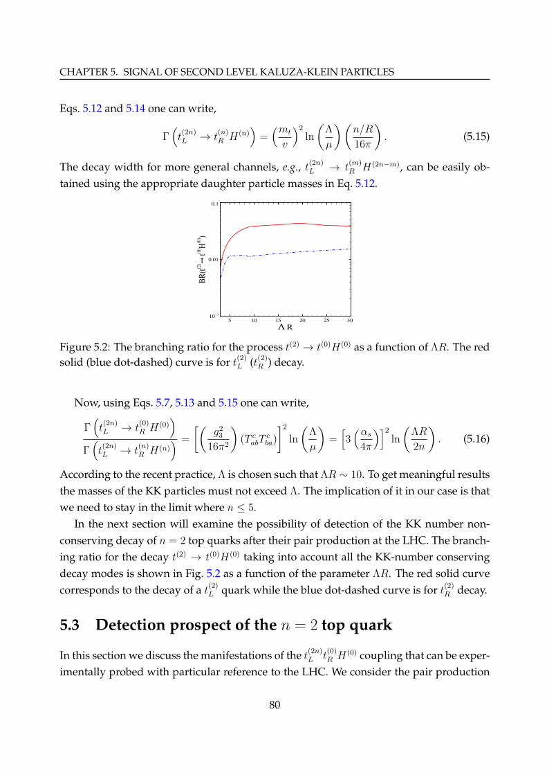
CHAPTER 5. SIGNAL OF SECOND LEVEL KALUZA-KLEIN PARTICLES
Eqs. 5.12 and 5.14 one can write,
Γ(t(2n)L → t
(n)R H(n)
)=(mt
v
)2
ln
(Λ
µ
)(n/R
16π
). (5.15)
The decay width for more general channels, e.g., t(2n)L → t
(m)R H(2n−m), can be easily ob-
tained using the appropriate daughter particle masses in Eq. 5.12.
BR(t(2
) → t(0
) H(0) )
10−3
0.01
0.1
Λ R5 10 15 20 25 30
Figure 5.2: The branching ratio for the process t(2) → t(0)H(0) as a function of ΛR. The redsolid (blue dot-dashed) curve is for t(2)
L (t(2)R ) decay.
Now, using Eqs. 5.7, 5.13 and 5.15 one can write,
Γ(t(2n)L → t
(0)R H(0)
)
Γ(t(2n)L → t
(n)R H(n)
) =
[(g2
3
16π2
)(T cabT
cba)
]2
ln
(Λ
µ
)=[3(αs
4π
)]2
ln
(ΛR
2n
). (5.16)
According to the recent practice, Λ is chosen such that ΛR ∼ 10. To get meaningful resultsthe masses of the KK particles must not exceed Λ. The implication of it in our case is thatwe need to stay in the limit where n ≤ 5.
In the next section will examine the possibility of detection of the KK number non-conserving decay of n = 2 top quarks after their pair production at the LHC. The branch-ing ratio for the decay t(2) → t(0)H(0) taking into account all the KK-number conservingdecay modes is shown in Fig. 5.2 as a function of the parameter ΛR. The red solid curvecorresponds to the decay of a t(2)
L quark while the blue dot-dashed curve is for t(2)R decay.
5.3 Detection prospect of the n = 2 top quark
In this section we discuss the manifestations of the t(2n)L t
(0)R H(0) coupling that can be exper-
imentally probed with particular reference to the LHC. We consider the pair production
80

5.3. DETECTION PROSPECT OF THE N = 2 TOP QUARK
of t(2)L,Rt
(2)L,R at the LHC and the subsequent decay of both of them through the t(2)
L,Rt(0)R,LH
(0)
coupling and compare this signal with the SM background. Assuming that both n = 2
top-quarks decay in the t(0)H(0) mode the signal consists of two top quarks6 and twoHiggs bosons such that the correct pairing leads to identical invariant masses for the twot(0)H(0) pairs. We estimate the Standard Model background for this channel and find it tobe insignificant, see the discussion below. However, with
√s = 13 TeV the signal is small
in number and inadequate for vindicating the strength of the coupling. On the otherhand, with the HL-LHC option with the same
√s with
∫Ldt = 3000 fb−1 the signal could
be viable. For the HE-LHC with√s = 33 TeV and
∫Ldt = 300 fb−1 the reach would be
more. The 100 TeV hadron Future Circular Collider (FCC) would surely do the best.
√s = 13 TeV√s = 33 TeV
σ(pp
→ t(2
) t(2) ) (
fb)
10−3
0.01
0.1
1
10
100
1000
1/R (GeV)600 800 1000 1200 1400
Figure 5.3: The production cross section for a t(2)t(2) pair at the LHC. The blue solid (reddashed) curve corresponds to
√s = 13 TeV (33 TeV).
We add the couplings of our concern in the CalcHEP implementation of mUED [54,165] to generate the events. A parton-level Monte Carlo has been utilized with theCTEQ6l [170] distribution functions. The renormalization scale (for αs) and the factor-ization scale (for the parton distributions) are both taken as 2n/R.
The production of the t(2)t(2) pair proceeds through gluon-gluon fusion – both s-channel and t-channel processes – as well as qq annihilation. We find that at the
√s
that we study the former dominate. The production cross sections for LHC running at√s = 13 TeV and in the future at 33 TeV are shown in Fig. 5.3.
The goal of this section is only to make a preliminary examination of this channel. So,we have refrained from including detailed detector simulation or indeed the subsequent
6Surely, one would be a top anti-quark but we forego this distinction for ease of presentation.
81

CHAPTER 5. SIGNAL OF SECOND LEVEL KALUZA-KLEIN PARTICLES
√s = 13 TeV
SM1/R = 600 GeV1/R = 800 GeV1/R = 1000 GeV1/R = 1200 GeV
dmtH
dσ (f
b/80
GeV
)
10−4
10−3
0.01
0.1
mtH (GeV)500 1000 1500 2000 2500 3000 3500
√s = 33 TeV
SM1/R = 600 GeV1/R = 800 GeV1/R = 1000 GeV1/R = 1200 GeV
dmtH
dσ (f
b/80
GeV
)
10−3
0.01
0.1
1
10
mtH (GeV)500 1000 1500 2000 2500 3000 3500 4000
Figure 5.4: The cross section for the (tH)(tH) signal at the LHC as a function of the t(0)H(0)
invariant mass. The histograms for different choices of 1/R (explained in the legend) andthe SM background (shown shaded) at the LHC running at
√s = 13 TeV (left) and 33 TeV
(right).
decays of the top-quark or the Higgs bosons. We incorporate these effects by appropriatedetection efficiency factors for these particles after applying kinematic cuts7. For all trackswe impose the following pT and rapidity η cuts:
pT > 25 GeV , |η| < 2.5 . (5.17)
In addition, all four tracks are required to be isolated. For any two tracks i, j we require:
∆Rij =√
(∆η)2ij + (∆φ)2
ij > 0.5 . (5.18)
From the surviving events we pick those for which there are two distinct t(0)H(0) pairsof the same invariant mass. We ensure that the pT of the two reconstructed t(2) are bal-anced to within 10%.
In Fig. 5.4 is shown the cross section for the above process as a function of the t(0)H(0)
invariant mass. In the left (right) panel are the results for√s = 13 (33) TeV. The histograms
correspond to the signal for 1/R = 600 GeV (red dotted), 800 GeV (green dashed), 1000GeV (blue solid), and 1200 GeV (pink dot-dashed). For both panels the SM background,shown shaded gray, is insignificant in the region of the signal. So, a signal of 10 eventswould be strong evidence for this model.
7The usage of these detection efficiencies, at least approximately, avoids the considerations of experi-mental signatures of the ttHH final states (number of jets etc.) and thereby bypasses the concerned combi-natorial problems associated with the counting of the final state jets.
82
5.4. CONCLUSION
The detection efficiency of boosted top quarks and Higgs bosons have been undermuch investigation in the literature. Using jet substructure features the tagging efficiencyof boosted top quarks with pT in the 800 - 1000 GeV range is estimated around εtop = 0.40-0.45 [171]. For a boosted Higgs boson similar analyses yield an efficiency of εh→bb = 0.94for the bb decay mode [172] which has a branching ratio of about 60%.
As seen from the left panel of Fig. 5.4, for√s = 13 TeV with 300 fb−1 integrated lumi-
nosity the detection is unlikely. For the lowest 1/R that we consider, namely 600 GeV, onehas around 30 events. Using the above-mentioned top quark and Higgs boson taggingefficiencies8 one is left with the signal of ((2/3)εtop)
2(0.6εh→bb)2 × 30 ∼ 1 event only. For
the high luminosity HL-LHC option (∫Ldt = 3000 fb−1) this will become a healthy 10-
event signal. However, with 1/R = 800 GeV the signal will fall to around 1 event. On theother hand, at a HE-LHC with
√s = 33 TeV (right panel of Fig. 5.4) the signal is enhanced
roughly by two orders of magnitude and could remain viable till 1/R = 1 TeV with∫Ldt =
3000 fb−1. We have checked that with a 100 TeV hadron FCC even for 100 fb−1 integratedluminosity this reach would go up to 1/R = 2.5 TeV for which we find 10 events.
5.4 Conclusion
In this chapter we have calculated the coupling of a 2n-level KK top-quark to a zero-mode top and a zero-mode Higgs boson in the universal extra-dimensional model. Sucha coupling violates KK-number but respects KK-parity and is induced by loop diagrams.The dominant contribution comes from n-level quark and gluon mediation. We evaluatethis coupling and show that it is independent of n.
We use this coupling to estimate the branching ratio of a second level KK-top quarkto this mode which has the advantage of a large phase space. Considering the pair pro-duction of such second level top quarks at the LHC with
√s = 13 TeV and 33 TeV we
examine the prospects of the detection of both of them in this decay mode. Our resultsare encouraging for the higher energy run.
8We conservatively include only the bb decay mode of the Higgs.
83

CHAPTER 5. SIGNAL OF SECOND LEVEL KALUZA-KLEIN PARTICLES
84

Chapter 6
Summary and conclusions
The physics of electroweak symmetry breaking in the standard model has been consol-idated by the discovery of Higgs boson. However, various other experimental observa-tions give rise to a clamant need for going beyond the SM. Among other incarnations ofnew physics, the idea of the existence of extra spatial dimensions is a fascinating possibil-ity in view of conceptual and phenomenological implications. In this thesis we considera particular class of theories which is known as the universal extra dimensional model.
Here we have considered this model in its basic as well as in a non-minimal version.The basic form is actually a higher dimensional version of SM, where all the particlescan propagate in the extra dimension, their Kaluza-Klein excitations have a simple massformula, and the couplings of these excitations are similar to the ones of the SM parti-cles. In the non-minimal avatar additional four-dimensional kinetic terms localized at thefixed points are incorporated. It has been investigated in this thesis how cosmologicalobservations and results from LHC can shed light on this model.
In Chapter 1 we briefly reviewed the SM and theoretical as well as experimental mo-tivations to go beyond this. In the later part of this chapter we introduced the basic fea-tures of extra dimensional models in the context of particle physics. The minimal andnon-minimal version of the UED model have been discussed in Chapter 2. After this wedescribe the new works that constitute the thesis.
• Various astrophysical observations indirectly proved the existence of dark matterwhich none of the known particles of SM can account for. One of the nice featuresof the UED model is that it predicts a suitable dark matter candidate. In Chapter 3we reviewed various observations that demand the existence of dark matter andalso the standard methodology of calculating different observables related to darkmatter. Later we examined how the dark matter candidate arising in the model
85

CHAPTER 6. SUMMARY AND CONCLUSIONS
fares when subjected to the observational constraints, namely the relic density anddirect detection constraints. It has been shown that while it can satisfy the relic den-sity data, it requires more sensitive direct detection experiments to consolidate itscandidature.
• The discovery of the Higgs boson at the LHC renews the enthusiasm in the field ofparticle physics which was otherwise long been wilted due to the non-observationof any new particle which was needed to understand the electroweak symmetrybreaking. The data, obtained at LHC, that led to the discovery also serve the pur-pose of judging many new physics scenarios beyond SM. Chapter 4 concentrateson these aspects. We showed that the non-minimal version of UED can do a betterjob in terms of relaxing the constraint on the compactification radius that is put inthe minimal version of the model from the Higgs data. However a detailed andrigorous collider study is imperative to assess the scenario in a thorough manner.
• In Chapter 5 we calculated the effective coupling of an even-numbered Kaluza-Klein top quark excitation to the zero mode top quark and a zero mode Higgs bosonin the UED model. Although such couplings are KK-number violating but they areKK-parity conserving and are induced by loop diagrams. We used this coupling toestimate the branching ratio of a second level top quark to a zero mode top and theHiggs boson. Finally we examined the prospects of verifying the theory throughthe detection of the second level top quark decays through this mode at the LHC.
LHC is being prepared for the next phase run with a higher energy. So it is the righttime to get prepared with the possible signals of alternative new physics scenarios. Theexploration of physics at such an unprecedented high scale of energy can very well ushersome major developments in the particle physics world. This thesis is just an humbleeffort to look for some of these aspects.
86

Bibliography
[1] R. Streater and A. Wightman, PCT, spin and statistics, and all that. PrincetonUniversity Press, Princeton, USA, 1989.
[2] Y. Nambu and G. Jona-Lasinio, Dynamical Model of Elementary Particles Based on anAnalogy with Superconductivity. 1., Phys.Rev. 122 (1961) 345–358.
[3] Y. Nambu and G. Jona-Lasinio, DYNAMICAL MODEL OF ELEMENTARYPARTICLES BASED ON AN ANALOGY WITH SUPERCONDUCTIVITY. II,Phys.Rev. 124 (1961) 246–254.
[4] J. Goldstone, Field Theories with Superconductor Solutions, Nuovo Cim. 19 (1961)154–164.
[5] J. Goldstone, A. Salam, and S. Weinberg, Broken Symmetries, Phys.Rev. 127 (1962)965–970.
[6] F. Englert and R. Brout, Broken Symmetry and the Mass of Gauge Vector Mesons,Phys.Rev.Lett. 13 (1964) 321–323.
[7] P. W. Higgs, Broken Symmetries and the Masses of Gauge Bosons, Phys.Rev.Lett. 13(1964) 508–509.
[8] G. Guralnik, C. Hagen, and T. Kibble, Global Conservation Laws and MasslessParticles, Phys.Rev.Lett. 13 (1964) 585–587.
[9] P. W. Higgs, Spontaneous Symmetry Breakdown without Massless Bosons, Phys.Rev. 145(1966) 1156–1163.
[10] T. Kibble, Symmetry breaking in nonAbelian gauge theories, Phys.Rev. 155 (1967)1554–1561.
[11] S. Glashow, Partial Symmetries of Weak Interactions, Nucl.Phys. 22 (1961) 579–588.
87

BIBLIOGRAPHY
[12] S. Weinberg, A Model of Leptons, Phys.Rev.Lett. 19 (1967) 1264–1266.
[13] A. Salam, Weak and Electromagnetic Interactions, Conf.Proc. C680519 (1968) 367–377.
[14] G. ’t Hooft, Renormalizable Lagrangians for Massive Yang-Mills Fields, Nucl.Phys. B35(1971) 167–188.
[15] G. ’t Hooft and M. Veltman, Regularization and Renormalization of Gauge Fields,Nucl.Phys. B44 (1972) 189–213.
[16] S. R. Coleman, There are no Goldstone bosons in two-dimensions, Commun.Math.Phys.31 (1973) 259–264.
[17] N. D. Mermin and H. Wagner, Absence of ferromagnetism or antiferromagnetism inone- or two-dimensional isotropic heisenberg models, Phys. Rev. Lett. 17 (Nov, 1966)1133–1136.
[18] P. C. Hohenberg, Existence of long-range order in one and two dimensions, Phys. Rev.158 (Jun, 1967) 383–386.
[19] J. Ellis and L. Álvarez-Gaumé, Eyes on a prize particle, Nature Physics 7 (2011) 2–3.
[20] ATLAS Collaboration, G. Aad et al., Observation of a new particle in the search for theStandard Model Higgs boson with the ATLAS detector at the LHC, Phys.Lett. B716(2012) 1–29, [arXiv:1207.7214].
[21] CMS Collaboration, S. Chatrchyan et al., Observation of a new boson at a mass of 125GeV with the CMS experiment at the LHC, Phys.Lett. B716 (2012) 30–61,[arXiv:1207.7235].
[22] R. Mohapatra, S. Antusch, K. Babu, G. Barenboim, M.-C. Chen, et al., Theory ofneutrinos: A White paper, Rept.Prog.Phys. 70 (2007) 1757–1867, [hep-ph/0510213].
[23] K. Abazajian, M. Acero, S. Agarwalla, A. Aguilar-Arevalo, C. Albright, et al., LightSterile Neutrinos: A White Paper, arXiv:1204.5379.
[24] G. Nordstrom, On the possibility of unifying the electromagnetic and the gravitationalfields, Phys.Z. 15 (1914) 504–506, [physics/0702221].
[25] T. Kaluza, On the Problem of Unity in Physics, Sitzungsber.Preuss.Akad.Wiss.Berlin(Math.Phys.) 1921 (1921) 966–972.
88
BIBLIOGRAPHY
[26] O. Klein, Quantum Theory and Five-Dimensional Theory of Relativity. (In German andEnglish), Z.Phys. 37 (1926) 895–906.
[27] E. Witten, Search for a Realistic Kaluza-Klein Theory, Nucl.Phys. B186 (1981) 412.
[28] I. Antoniadis, A Possible new dimension at a few TeV, Phys.Lett. B246 (1990) 377–384.
[29] N. Arkani-Hamed, S. Dimopoulos, and G. Dvali, The Hierarchy problem and newdimensions at a millimeter, Phys.Lett. B429 (1998) 263–272, [hep-ph/9803315].
[30] L. Randall and R. Sundrum, A Large mass hierarchy from a small extra dimension,Phys.Rev.Lett. 83 (1999) 3370–3373, [hep-ph/9905221].
[31] L. Randall and R. Sundrum, An Alternative to compactification, Phys.Rev.Lett. 83(1999) 4690–4693, [hep-th/9906064].
[32] T. Appelquist, H.-C. Cheng, and B. A. Dobrescu, Bounds on universal extradimensions, Phys.Rev. D64 (2001) 035002, [hep-ph/0012100].
[33] D. Bailin and A. Love, KALUZA-KLEIN THEORIES, Rept.Prog.Phys. 50 (1987)1087–1170.
[34] Particle Data Group Collaboration, K. A. Olive et al., Review of Particle Physics(RPP), Chin.Phys. C38 (2014) 090001.
[35] V. Rubakov and M. Shaposhnikov, Do We Live Inside a Domain Wall?, Phys.Lett.B125 (1983) 136–138.
[36] V. Rubakov and M. Shaposhnikov, Extra Space-Time Dimensions: Towards a Solutionto the Cosmological Constant Problem, Phys.Lett. B125 (1983) 139.
[37] R. Sundrum, Tasi 2004 lectures: To the fifth dimension and back, hep-th/0508134.
[38] T. Gherghetta, TASI Lectures on a Holographic View of Beyond the Standard ModelPhysics, arXiv:1008.2570.
[39] https://atlas.web.cern.ch/Atlas/GROUPS/PHYSICS/
CombinedSummaryPlots/EXOTICS/ATLAS_Exotics_Summary/history.
html.
[40] https://twiki.cern.ch/twiki/bin/view/CMSPublic/
PhysicsResultsEXO#CMS_EXO_Summary_of_Mass_Limits.
89

BIBLIOGRAPHY
[41] T. Appelquist, B. A. Dobrescu, E. Ponton, and H.-U. Yee, Proton stability insix-dimensions, Phys.Rev.Lett. 87 (2001) 181802, [hep-ph/0107056].
[42] B. A. Dobrescu and E. Poppitz, Number of fermion generations derived from anomalycancellation, Phys.Rev.Lett. 87 (2001) 031801, [hep-ph/0102010].
[43] K. R. Dienes, E. Dudas, and T. Gherghetta, Extra space-time dimensions andunification, Phys.Lett. B436 (1998) 55–65, [hep-ph/9803466].
[44] K. R. Dienes, E. Dudas, and T. Gherghetta, Grand unification at intermediate massscales through extra dimensions, Nucl.Phys. B537 (1999) 47–108, [hep-ph/9806292].
[45] A. Perez-Lorenzana and R. Mohapatra, Effect of extra dimensions on gauge couplingunification, Nucl.Phys. B559 (1999) 255, [hep-ph/9904504].
[46] G. Altarelli and F. Feruglio, SU(5) grand unification in extra dimensions and protondecay, Phys.Lett. B511 (2001) 257–264, [hep-ph/0102301].
[47] D. Hooper and S. Profumo, Dark matter and collider phenomenology of universal extradimensions, Phys.Rept. 453 (2007) 29–115, [hep-ph/0701197].
[48] H.-C. Cheng, K. T. Matchev, and M. Schmaltz, Bosonic supersymmetry? Gettingfooled at the CERN LHC, Phys.Rev. D66 (2002) 056006, [hep-ph/0205314].
[49] J. M. Smillie and B. R. Webber, Distinguishing spins in supersymmetric and universalextra dimension models at the large hadron collider, JHEP 0510 (2005) 069,[hep-ph/0507170].
[50] B. Dobrescu, TASI 2008: Introduction to extra dimensions: ADD, UED, RS, and dual toTC, etc, .
[51] R. S. Chivukula, D. A. Dicus, and H.-J. He, Unitarity of compactified five-dimensionalYang-Mills theory, Phys.Lett. B525 (2002) 175–182, [hep-ph/0111016].
[52] C. Csaki, C. Grojean, H. Murayama, L. Pilo, and J. Terning, Gauge theories on aninterval: Unitarity without a Higgs, Phys.Rev. D69 (2004) 055006,[hep-ph/0305237].
[53] C. Schwinn, Higgsless fermion masses and unitarity, Phys.Rev. D69 (2004) 116005,[hep-ph/0402118].
90

BIBLIOGRAPHY
[54] A. Datta, K. Kong, and K. T. Matchev, Minimal Universal Extra Dimensions inCalcHEP/CompHEP, New J.Phys. 12 (2010) 075017, [arXiv:1002.4624].
[55] A. Datta, U. K. Dey, A. Raychaudhuri, and A. Shaw, Boundary Localized Terms inUniversal Extra-Dimensional Models through a Dark Matter perspective, Phys.Rev. D88(2013) 016011, [arXiv:1305.4507].
[56] U. K. Dey and T. S. Ray, Constraining minimal and nonminimal universal extradimension models with Higgs couplings, Phys.Rev. D88 (2013), no. 5 056016,[arXiv:1305.1016].
[57] U. K. Dey and A. Raychaudhuri, KK-number non-conserving decays: Signal of n = 2excitations of Extra-Dimensional Models at the LHC, arXiv:1410.1463.
[58] H.-C. Cheng, K. T. Matchev, and M. Schmaltz, Radiative corrections to Kaluza-Kleinmasses, Phys.Rev. D66 (2002) 036005, [hep-ph/0204342].
[59] H. Georgi, A. K. Grant, and G. Hailu, Brane couplings from bulk loops, Phys.Lett.B506 (2001) 207–214, [hep-ph/0012379].
[60] Particle Data Group Collaboration, J. Beringer et al., Review of Particle Physics(RPP), Phys.Rev. D86 (2012) 010001.
[61] F. del Aguila and J. Santiago, Low-energy constraints on orbifold models,Nucl.Phys.Proc.Suppl. 116 (2003) 326–330, [hep-ph/0212205].
[62] F. del Aguila, M. Perez-Victoria, and J. Santiago, Bulk fields with general brane kineticterms, JHEP 0302 (2003) 051, [hep-th/0302023].
[63] F. del Aguila, M. Perez-Victoria, and J. Santiago, Some consequences of brane kineticterms for bulk fermions, hep-ph/0305119.
[64] F. del Aguila, M. Perez-Victoria, and J. Santiago, Bulk fields with brane terms,Eur.Phys.J. C33 (2004) S773–S775, [hep-ph/0310352].
[65] F. del Aguila, M. Perez-Victoria, and J. Santiago, Physics of brane kinetic terms, ActaPhys.Polon. B34 (2003) 5511–5522, [hep-ph/0310353].
[66] T. Flacke, A. Menon, and D. J. Phalen, Non-minimal universal extra dimensions,Phys.Rev. D79 (2009) 056009, [arXiv:0811.1598].
91

BIBLIOGRAPHY
[67] A. Datta, K. Nishiwaki, and S. Niyogi, Non-minimal Universal Extra Dimensions withBrane Local Terms: The Top Quark Sector, JHEP 1401 (2014) 104,[arXiv:1310.6994].
[68] M. S. Carena, T. M. Tait, and C. Wagner, Branes and orbifolds are opaque, ActaPhys.Polon. B33 (2002) 2355, [hep-ph/0207056].
[69] A. Datta, U. K. Dey, A. Shaw, and A. Raychaudhuri, Universal Extra-DimensionalModels with Boundary Localized Kinetic Terms: Probing at the LHC, Phys.Rev. D87(2013) 076002, [arXiv:1205.4334].
[70] A. Datta, A. Raychaudhuri, and A. Shaw, LHC limits on KK-parity non-conservationin the strong sector of universal extra-dimension models, Phys.Lett. B730 (2014) 42–49,[arXiv:1310.2021].
[71] A. Shaw, KK-parity non-conservation in UED confronts LHC data,arXiv:1405.3139.
[72] A. Datta, K. Nishiwaki, and S. Niyogi, Non-minimal Universal Extra Dimensions: TheStrongly Interacting Sector at the Large Hadron Collider, JHEP 1211 (2012) 154,[arXiv:1206.3987].
[73] T. Flacke, K. Kong, and S. C. Park, Phenomenology of Universal Extra Dimensions withBulk-Masses and Brane-Localized Terms, JHEP 1305 (2013) 111, [arXiv:1303.0872].
[74] Planck Collaboration, P. Ade et al., Planck 2013 results. XVI. Cosmologicalparameters, arXiv:1303.5076.
[75] E. W. Kolb and M. S. Turner, The Early Universe, Front.Phys. 69 (1990) 1–547.
[76] G. Jungman, M. Kamionkowski, and K. Griest, Supersymmetric dark matter,Phys.Rept. 267 (1996) 195–373, [hep-ph/9506380].
[77] L. Bergstrom, Nonbaryonic dark matter: Observational evidence and detection methods,Rept.Prog.Phys. 63 (2000) 793, [hep-ph/0002126].
[78] G. Bertone, D. Hooper, and J. Silk, Particle dark matter: Evidence, candidates andconstraints, Phys.Rept. 405 (2005) 279–390, [hep-ph/0404175].
[79] H. Murayama, Physics Beyond the Standard Model and Dark Matter,arXiv:0704.2276.
92

BIBLIOGRAPHY
[80] G. Bertone, J. Silk, B. Moore, J. Diemand, J. Bullock, et al., Particle Dark Matter:Observations, Models and Searches, .
[81] S. Profumo, TASI 2012 Lectures on Astrophysical Probes of Dark Matter,arXiv:1301.0952.
[82] F. Zwicky, Die Rotverschiebung von extragalaktischen Nebeln, Helv.Phys.Acta 6 (1933)110–127.
[83] R. Tully and J. Fisher, A New method of determining distances to galaxies,Astron.Astrophys. 54 (1977) 661–673.
[84] M. Aaronson, J. Huchra, and J. Mould, The infrared luminosity/H I velocity-widthrelation and its application to the distance scale, ApJ 229 (Apr., 1979) 1–13.
[85] J. A. Tyson, G. P. Kochanski, and I. P. Dell’Antonio, Detailed mass map ofCL0024+1654 from strong lensing, Astrophys.J. 498 (1998) L107,[astro-ph/9801193].
[86] R. Massey, J. Rhodes, R. Ellis, N. Scoville, A. Leauthaud, et al., Dark matter mapsreveal cosmic scaffolding, Nature 445 (2007) 286, [astro-ph/0701594].
[87] D. Clowe, M. Bradac, A. H. Gonzalez, M. Markevitch, S. W. Randall, et al., A directempirical proof of the existence of dark matter, Astrophys.J. 648 (2006) L109–L113,[astro-ph/0608407].
[88] G. Hinshaw, D. Larson, E. Komatsu, D. N. Spergel, C. L. Bennett, J. Dunkley, M. R.Nolta, M. Halpern, R. S. Hill, N. Odegard, L. Page, K. M. Smith, J. L. Weiland,B. Gold, N. Jarosik, A. Kogut, M. Limon, S. S. Meyer, G. S. Tucker, E. Wollack, andE. L. Wright, Nine-year Wilkinson Microwave Anisotropy Probe (WMAP) Observations:Cosmological Parameter Results, ApJS 208 (Oct., 2013) 19, [arXiv:1212.5226].
[89] E. Otten and C. Weinheimer, Neutrino mass limit from tritium beta decay,Rept.Prog.Phys. 71 (2008) 086201, [arXiv:0909.2104].
[90] S. Tremaine and J. Gunn, Dynamical Role of Light Neutral Leptons in Cosmology,Phys.Rev.Lett. 42 (1979) 407–410.
[91] K. Griest, Galactic Microlensing as a Method of Detecting Massive Compact HaloObjects, Astrophys.J. 366 (1991) 412–421.
93

BIBLIOGRAPHY
[92] B. J. Carr, Baryonic dark matter, Ann.Rev.Astron.Astrophys. 32 (1994) 531–590.
[93] L. Bergstrom, Dark Matter Candidates, New J.Phys. 11 (2009) 105006,[arXiv:0903.4849].
[94] R. Peccei and H. R. Quinn, CP Conservation in the Presence of Instantons,Phys.Rev.Lett. 38 (1977) 1440–1443.
[95] M. S. Turner, Windows on the Axion, Phys.Rept. 197 (1990) 67–97.
[96] G. G. Raffelt, Astrophysical methods to constrain axions and other novel particlephenomena, Phys.Rept. 198 (1990) 1–113.
[97] L. Visinelli and P. Gondolo, Dark Matter Axions Revisited, Phys.Rev. D80 (2009)035024, [arXiv:0903.4377].
[98] P. Sikivie, Dark matter axions, Int.J.Mod.Phys. A25 (2010) 554–563,[arXiv:0909.0949].
[99] M. Archidiacono, S. Hannestad, A. Mirizzi, G. Raffelt, and Y. Y. Wong, Axion hotdark matter bounds after Planck, JCAP 1310 (2013) 020, [arXiv:1307.0615].
[100] K. S. Jeong, M. Kawasaki, and F. Takahashi, Axions as Hot and Cold Dark Matter,JCAP 1402 (2014) 046, [arXiv:1310.1774].
[101] E. Di Valentino, E. Giusarma, M. Lattanzi, A. Melchiorri, and O. Mena, Axion colddark matter: status after Planck and BICEP2, arXiv:1405.1860.
[102] S. Profumo, Neutralino dark matter: where particle physics meets cosmology . PhDthesis, UC, Santa Cruz & UC, Santa Cruz, Inst. Part. Phys., 2005.
[103] L. Calibbi, J. M. Lindert, T. Ota, and Y. Takanishi, Cornering light Neutralino DarkMatter at the LHC, JHEP 1310 (2013) 132, [arXiv:1307.4119].
[104] G. Bélanger, G. Drieu La Rochelle, B. Dumont, R. M. Godbole, S. Kraml, et al., LHCconstraints on light neutralino dark matter in the MSSM, Phys.Lett. B726 (2013)773–780, [arXiv:1308.3735].
[105] T. Han, Z. Liu, and S. Su, Light Neutralino Dark Matter: Direct/Indirect Detection andCollider Searches, arXiv:1406.1181.
94

BIBLIOGRAPHY
[106] L. Lopez Honorez, E. Nezri, J. F. Oliver, and M. H. Tytgat, The Inert Doublet Model:An Archetype for Dark Matter, JCAP 0702 (2007) 028, [hep-ph/0612275].
[107] A. Arhrib, Y.-L. S. Tsai, Q. Yuan, and T.-C. Yuan, An Updated Analysis of Inert HiggsDoublet Model in light of the Recent Results from LUX, PLANCK, AMS-02 and LHC,arXiv:1310.0358.
[108] G. Servant and T. M. Tait, Is the lightest Kaluza-Klein particle a viable dark mattercandidate?, Nucl.Phys. B650 (2003) 391–419, [hep-ph/0206071].
[109] G. Servant and T. M. Tait, Elastic scattering and direct detection of Kaluza-Klein darkmatter, New J.Phys. 4 (2002) 99, [hep-ph/0209262].
[110] K. Kong and K. T. Matchev, Precise calculation of the relic density of Kaluza-Klein darkmatter in universal extra dimensions, JHEP 0601 (2006) 038, [hep-ph/0509119].
[111] M. Kakizaki, S. Matsumoto, Y. Sato, and M. Senami, Relic abundance of LKP darkmatter in UED model including effects of second KK resonances, Nucl.Phys. B735 (2006)84–95, [hep-ph/0508283].
[112] M. Kakizaki, S. Matsumoto, Y. Sato, and M. Senami, Significant effects of second KKparticles on LKP dark matter physics, Phys.Rev. D71 (2005) 123522,[hep-ph/0502059].
[113] T. Flacke, D. Hooper, and J. March-Russell, Improved bounds on universal extradimensions and consequences for LKP dark matter, Phys.Rev. D73 (2006) 095002,[hep-ph/0509352].
[114] F. Burnell and G. D. Kribs, The Abundance of Kaluza-Klein dark matter withcoannihilation, Phys.Rev. D73 (2006) 015001, [hep-ph/0509118].
[115] T. Flacke and D. W. Maybury, Constraints on UED KK-neutrino dark matter frommagnetic dipole moments, Int.J.Mod.Phys. D16 (2007) 1593–1600,[hep-ph/0601161].
[116] M. Kakizaki, S. Matsumoto, and M. Senami, Relic abundance of dark matter in theminimal universal extra dimension model, Phys.Rev. D74 (2006) 023504,[hep-ph/0605280].
95

BIBLIOGRAPHY
[117] S. Arrenberg, L. Baudis, K. Kong, K. T. Matchev, and J. Yoo, Kaluza-Klein DarkMatter: Direct Detection vis-a-vis LHC, Phys.Rev. D78 (2008) 056002,[arXiv:0805.4210].
[118] G. Belanger, M. Kakizaki, and A. Pukhov, Dark matter in UED: The Role of the secondKK level, JCAP 1102 (2011) 009, [arXiv:1012.2577].
[119] S. Arrenberg, L. Baudis, K. Kong, K. T. Matchev, and J. Yoo, Kaluza-Klein DarkMatter: Direct Detection vis-a-vis LHC (2013 update), arXiv:1307.6581.
[120] T. Flacke, Phenomenology of dark matter in non-minimal UED, AIP Conf.Proc. 1200(2010) 583–586.
[121] J. D. Wells, Annihilation cross-sections for relic densities in the low velocity limit,hep-ph/9404219.
[122] M. Srednicki, R. Watkins, and K. A. Olive, Calculations of Relic Densities in the EarlyUniverse, Nucl.Phys. B310 (1988) 693.
[123] K. Griest and D. Seckel, Three exceptions in the calculation of relic abundances,Phys.Rev. D43 (1991) 3191–3203.
[124] J. L. Feng, A. Rajaraman, and F. Takayama, Graviton cosmology in universal extradimensions, Phys.Rev. D68 (2003) 085018, [hep-ph/0307375].
[125] S. Matsumoto, J. Sato, M. Senami, and M. Yamanaka, Solving cosmological problem inuniversal extra dimension models by introducing Dirac neutrino, Phys.Lett. B647 (2007)466–471, [hep-ph/0607331].
[126] S. Matsumoto, J. Sato, M. Senami, and M. Yamanaka, Relic abundance of dark matterin universal extra dimension models with right-handed neutrinos, Phys.Rev. D76 (2007)043528, [arXiv:0705.0934].
[127] S. Matsumoto, J. Sato, M. Yamanaka, and M. Senami, Introducing neutrino mass intouniversal extra dimension models and solving cosmological problem, Int.J.Mod.Phys. E16(2007) 1571–1582.
[128] H. Melbeus, A. Merle, and T. Ohlsson, Higgs Dark Matter in UEDs: A Good WIMPwith Bad Detection Prospects, Phys.Lett. B715 (2012) 164–169, [arXiv:1204.5186].
96
BIBLIOGRAPHY
[129] J. Bonnevier, H. Melbeus, A. Merle, and T. Ohlsson, Monoenergetic Gamma-Raysfrom Non-Minimal Kaluza-Klein Dark Matter Annihilations, Phys.Rev. D85 (2012)043524, [arXiv:1104.1430].
[130] WMAP Collaboration, J. Dunkley et al., Five-Year Wilkinson Microwave AnisotropyProbe (WMAP) Observations: Likelihoods and Parameters from the WMAP data,Astrophys.J.Suppl. 180 (2009) 306–329, [arXiv:0803.0586].
[131] http://www.mpi-hd.mpg.de/lin/research_DM.en.html.
[132] C. Munoz, Dark matter detection in the light of recent experimental results,Int.J.Mod.Phys. A19 (2004) 3093–3170, [hep-ph/0309346].
[133] P. Salati, Indirect and direct dark matter detection, PoS CARGESE2007 (2007) 009.
[134] M. W. Goodman and E. Witten, Detectability of Certain Dark Matter Candidates,Phys.Rev. D31 (1985) 3059.
[135] CDMS II, Z. Ahmed, D. S. Akerib, S. Arrenberg, C. N. Bailey, D. Balakishiyeva,L. Baudis, D. A. Bauer, P. L. Brink, T. Bruch, R. Bunker, B. Cabrera, D. O. Caldwell,J. Cooley, P. Cushman, M. Daal, F. DeJongh, M. R. Dragowsky, L. Duong,S. Fallows, E. Figueroa-Feliciano, J. Filippini, M. Fritts, S. R. Golwala, D. R. Grant,J. Hall, R. Hennings-Yeomans, S. A. Hertel, D. Holmgren, L. Hsu, M. E. Huber,O. Kamaev, M. Kiveni, M. Kos, S. W. Leman, R. Mahapatra, V. Mandic, K. A.McCarthy, N. Mirabolfathi, D. Moore, H. Nelson, R. W. Ogburn, A. Phipps,M. Pyle, X. Qiu, E. Ramberg, W. Rau, A. Reisetter, T. Saab, B. Sadoulet, J. Sander,R. W. Schnee, D. N. Seitz, B. Serfass, K. M. Sundqvist, M. Tarka, P. Wikus, S. Yellin,J. Yoo, B. A. Young, and J. Zhang, Dark Matter Search Results from the CDMS IIExperiment, Science 327 (Mar., 2010) 1619–, [arXiv:0912.3592].
[136] EDELWEISS, E. Armengaud, C. Augier, A. Benoît, L. Bergé, J. Blümer,A. Broniatowski, V. Brudanin, B. Censier, G. Chardin, M. Chapellier, F. Charlieux,P. Coulter, G. A. Cox, X. Defay, M. de Jesus, Y. Dolgorouki, J. Domange,L. Dumoulin, K. Eitel, D. Filosofov, N. Fourches, J. Gascon, G. Gerbier, J. Gironnet,M. Gros, S. Henry, S. Hervé, A. Juillard, H. Kluck, V. Kozlov, H. Kraus, V. A.Kudryavtsev, P. Loaiza, S. Marnieros, X.-F. Navick, C. Nones, E. Olivieri, P. Pari,L. Pattavina, B. Paul, M. Robinson, S. Rozov, V. Sanglard, B. Schmidt, S. Scorza,S. Semikh, A. S. Torrento-Coello, L. Vagneron, M.-A. Verdier, R. J. Walker, and
97

BIBLIOGRAPHY
E. Yakushev, Final results of the EDELWEISS-II WIMP search using a 4-kg array ofcryogenic germanium detectors with interleaved electrodes, Physics Letters B 702 (Aug.,2011) 329–335, [arXiv:1103.4070].
[137] G. Angloher, M. Bauer, I. Bavykina, A. Bento, C. Bucci, C. Ciemniak, G. Deuter,F. von Feilitzsch, D. Hauff, P. Huff, C. Isaila, J. Jochum, M. Kiefer, M. Kimmerle,J.-C. Lanfranchi, F. Petricca, S. Pfister, W. Potzel, F. Pröbst, F. Reindl, S. Roth,K. Rottler, C. Sailer, K. Schäffner, J. Schmaler, S. Scholl, W. Seidel, M. v. Sivers,L. Stodolsky, C. Strandhagen, R. Strauß, A. Tanzke, I. Usherov, S. Wawoczny,M. Willers, and A. Zöller, Results from 730 kg days of the CRESST-II Dark Mattersearch, European Physical Journal C 72 (Apr., 2012) 1971, [arXiv:1109.0702].
[138] DAMA Collaboration, R. Bernabei et al., First results from DAMA/LIBRA and thecombined results with DAMA/NaI, Eur.Phys.J. C56 (2008) 333–355,[arXiv:0804.2741].
[139] E. Aprile, E. Baltz, A. Curioni, K.-L. Giboni, C. Hailey, et al., XENON: A 1 Tonneliquid xenon experiment for a sensitive dark matter search, astro-ph/0207670.
[140] E. Aprile, M. Alfonsi, K. Arisaka, F. Arneodo, C. Balan, L. Baudis, B. Bauermeister,A. Behrens, P. Beltrame, K. Bokeloh, E. Brown, G. Bruno, R. Budnik, J. M. R.Cardoso, W.-T. Chen, B. Choi, D. Cline, A. P. Colijn, H. Contreras, J. P. Cussonneau,M. P. Decowski, E. Duchovni, S. Fattori, A. D. Ferella, W. Fulgione, F. Gao,M. Garbini, C. Ghag, K.-L. Giboni, L. W. Goetzke, C. Grignon, E. Gross,W. Hampel, F. Kaether, A. Kish, J. Lamblin, H. Landsman, R. F. Lang, M. LeCalloch, C. Levy, K. E. Lim, Q. Lin, S. Lindemann, M. Lindner, J. A. M. Lopes,K. Lung, T. Marrodán Undagoitia, F. V. Massoli, A. J. Melgarejo Fernandez,Y. Meng, A. Molinario, E. Nativ, K. Ni, U. Oberlack, S. E. A. Orrigo, E. Pantic,R. Persiani, G. Plante, N. Priel, A. Rizzo, S. Rosendahl, J. M. F. dos Santos,G. Sartorelli, J. Schreiner, M. Schumann, L. Scotto Lavina, P. R. Scovell, M. Selvi,P. Shagin, H. Simgen, A. Teymourian, D. Thers, O. Vitells, H. Wang, M. Weber, andC. Weinheimer, Dark Matter Results from 225 Live Days of XENON100 Data, PhysicalReview Letters 109 (Nov., 2012) 181301, [arXiv:1207.5988].
[141] LUX Collaboration, D. Akerib et al., First results from the LUX dark matter experimentat the Sanford Underground Research Facility, Phys.Rev.Lett. 112 (2014) 091303,[arXiv:1310.8214].
98

BIBLIOGRAPHY
[142] H.-C. Cheng, J. L. Feng, and K. T. Matchev, Kaluza-Klein dark matter, Phys.Rev.Lett.89 (2002) 211301, [hep-ph/0207125].
[143] EDELWEISS Collaboration, A. Benoit et al., First results of the EDELWEISS WIMPsearch using a 320-g heat-and-ionization Ge detector, Phys.Lett. B513 (2001) 15–22,[astro-ph/0106094].
[144] CDMS Collaboration, D. Abrams et al., Exclusion limits on the WIMP nucleoncross-section from the cryogenic dark matter search, Phys.Rev. D66 (2002) 122003,[astro-ph/0203500].
[145] T. Flacke, A. Menon, D. Hooper, and K. Freese, Kaluza-Klein Dark Matter AndNeutrinos From Annihilation In The Sun, arXiv:0908.0899.
[146] XENON100 Collaboration, E. Aprile et al., Limits on spin-dependent WIMP-nucleoncross sections from 225 live days of XENON100 data, Phys.Rev.Lett. 111 (2013), no. 2021301, [arXiv:1301.6620].
[147] ATLAS Collaboration, G. Aad et al., Evidence for the spin-0 nature of the Higgs bosonusing ATLAS data, Phys.Lett. B726 (2013) 120–144, [arXiv:1307.1432].
[148] ATLAS Collaboration, Measurements of the properties of the Higgs-like boson in thefour lepton decay channel with the ATLAS detector using 25 fb−1 of proton-protoncollision data, .
[149] A. Freitas and P. Schwaller, Higgs CP Properties From Early LHC Data, Phys.Rev. D87(2013), no. 5 055014, [arXiv:1211.1980].
[150] A. Djouadi, R. Godbole, B. Mellado, and K. Mohan, Probing the spin-parity of theHiggs boson via jet kinematics in vector boson fusion, Phys.Lett. B723 (2013) 307–313,[arXiv:1301.4965].
[151] A. Djouadi and G. Moreau, The couplings of the Higgs boson and its CP properties fromfits of the signal strengths and their ratios at the 7+8 TeV LHC, Eur.Phys.J. C73 (2013)2512, [arXiv:1303.6591].
[152] M. R. Buckley and D. Hooper, Are There Hints of Light Stops in Recent Higgs SearchResults?, Phys.Rev. D86 (2012) 075008, [arXiv:1207.1445].
99

BIBLIOGRAPHY
[153] A. Djouadi, The Anatomy of electro-weak symmetry breaking. I: The Higgs boson in thestandard model, Phys.Rept. 457 (2008) 1–216, [hep-ph/0503172].
[154] G. Cacciapaglia, A. Deandrea, and J. Llodra-Perez, Higgs→ Gamma Gamma beyondthe Standard Model, JHEP 0906 (2009) 054, [arXiv:0901.0927].
[155] M. Spira, A. Djouadi, D. Graudenz, and P. Zerwas, Higgs boson production at theLHC, Nucl.Phys. B453 (1995) 17–82, [hep-ph/9504378].
[156] J. Ellis and T. You, Updated Global Analysis of Higgs Couplings, JHEP 1306 (2013) 103,[arXiv:1303.3879].
[157] A. Datta and S. Raychaudhuri, Vacuum Stability Constraints and LHC Searches for aModel with a Universal Extra Dimension, Phys.Rev. D87 (2013), no. 3 035018,[arXiv:1207.0476].
[158] G. Belanger, A. Belyaev, M. Brown, M. Kakizaki, and A. Pukhov, Testing MinimalUniversal Extra Dimensions Using Higgs Boson Searches at the LHC, Phys.Rev. D87(2013) 016008, [arXiv:1207.0798].
[159] T. Kakuda, K. Nishiwaki, K.-y. Oda, and R. Watanabe, Universal extra dimensionsafter Higgs discovery, Phys.Rev. D88 (2013) 035007, [arXiv:1305.1686].
[160] T. Kakuda, K. Nishiwaki, K.-y. Oda, and R. Watanabe, Constraint on Universal ExtraDimensions from scalar boson searches, arXiv:1305.1874.
[161] A. Datta, A. Patra, and S. Raychaudhuri, Higgs Boson Decay Constraints on a Modelwith a Universal Extra Dimension, Phys.Rev. D89 (2014) 093008,[arXiv:1311.0926].
[162] F. J. Petriello, Kaluza-Klein effects on Higgs physics in universal extra dimensions, JHEP0205 (2002) 003, [hep-ph/0204067].
[163] A. Datta and S. K. Rai, Identifying the contributions of universal extra dimensions in theHiggs sector at linear e+ e- colliders, Int.J.Mod.Phys. A23 (2008) 519–528,[hep-ph/0509277].
[164] P. Bandyopadhyay, B. Bhattacherjee, and A. Datta, Search for Higgs bosons of theUniversal Extra Dimensions at the Large Hadron Collider, JHEP 1003 (2010) 048,[arXiv:0909.3108].
100

BIBLIOGRAPHY
[165] A. Belyaev, M. Brown, J. Moreno, and C. Papineau, Discovering Minimal UniversalExtra Dimensions (MUED) at the LHC, JHEP 1306 (2013) 080, [arXiv:1212.4858].
[166] L. Edelhäuser, T. Flacke, and M. Krämer, Constraints on models with universal extradimensions from dilepton searches at the LHC, JHEP 1308 (2013) 091,[arXiv:1302.6076].
[167] M. Blennow, H. Melbeus, T. Ohlsson, and H. Zhang, RG running in a minimal UEDmodel in light of recent LHC Higgs mass bounds, Phys.Lett. B712 (2012) 419–424,[arXiv:1112.5339].
[168] D0 Collaboration, V. M. Abazov et al., Precision measurement of the top-quark mass inlepton+jets final states, Phys.Rev.Lett. 113 (2014) 032002, [arXiv:1405.1756].
[169] G. Passarino and M. Veltman, One Loop Corrections for e+ e- Annihilation Into mu+mu- in the Weinberg Model, Nucl.Phys. B160 (1979) 151.
[170] J. Pumplin, D. Stump, J. Huston, H. Lai, P. M. Nadolsky, et al., New generation ofparton distributions with uncertainties from global QCD analysis, JHEP 0207 (2002) 012,[hep-ph/0201195].
[171] D. E. Kaplan, K. Rehermann, M. D. Schwartz, and B. Tweedie, Top Tagging: AMethod for Identifying Boosted Hadronically Decaying Top Quarks, Phys.Rev.Lett. 101(2008) 142001, [arXiv:0806.0848].
[172] M. Backovic, T. Flacke, J. H. Kim, and S. J. Lee, Boosted Event Topologies from TeVScale Light Quark Composite Partners, arXiv:1410.8131.
101