179

Some Topical Variational Geometry Problems in Computer Graphics

G.N. Newsam.

Abstracto Smooth interpolation of arbitrary curves and surfaces is a major problem in computer graphics. There are very successful variational formulations of similar problems in smooth interpolation of arbitrary functions; these have given rise to the (linear) theory of splines. However, there appears to be as yet no equivalent useful formulation of the general problem, so present computer graphics algorithms for cunres and surfaces use somewhat ad hoc extensions of the linear results based on parametric representations of splines and surface patches. The paper briefly describes the present state of affairs in the hope that variational geometers will pick up on some of these unsolved problems and develop a coherent theory of smooth interpolation of arbitrary geometrical objects. If such a theory can be developed, it may possibly revolutionize computer graphics.

! . Introduction.

Computer graphics is one of the many amazingly fast growing technologies spawned in the last

two decades (see [4] for a general reference). Apple's Macintosh brought 2D graphical

interfaces to the masses, and standard workstations will soon feature interfaces that simulate

reality with full 3D graphics. This has been brought to fruition by perhaps the most intensive

application of geometry ever, but has been carried out mainly by engineers and computer

scientists; surprisingly little has been done by geometers. This paper outlines some pressing

problems in the field in the hope of enticing variational geometers to take a more active role in

their solution.

The problems described here revolve around construction of smooth curves and surfaces

subject to constraints, the most common being that they interpolate a given set of points. A

large family of smooth interpolants of functions (the linear splines) are naturally defined

through variational forms, yet there seem to be no formulations with equivalent explanatory

power for general smooth interpolants. The standard consnuctions used in computer graphics

are therefore based on parametric splineso Linear splines are easy to compute but result in

coordinate dependent approximations, while parametric splines depend strongly on the chosen

parameterization. In contrast, a general variational formulation holds the promise of a truly

180

coordinate independent construction, but results so far have been disappointing. The hope is

that variational geometers have both the insight and the tools to remedy this situation.

The question of what is the "correct" construction is of much more than academic interest.

Considerable effort is put into implementing constructions in silicon so that they will run as fast

as possible, and efficient constructions can greatly reduce the number of nodes needed to

accurately represent a curve or surface. At present graphics chips automatically approximate

curves or surfaces with geometric constructions such as lines, arcs of conics, Bezier curves and

NURBS (non-uniform rational B-splines). There is as yet no compelling justification,

however, for any particular approximation so the door is still open to new constructions of

proven merit. Unfortunately, with the increasing trend towards adoption of standards there is a

real possibility that existing constructions may soon be chosen as the basis of a future set of

graphics approximation standards. This would erect a formidable barrier to further innovation,

no matter how beneficial it might be. Thus the whole issue of smooth interpolants needs to be

settled quickly. It may be that variational geometers have in fact already done so (I make no

claim to be familiar with the literature in this field), in which case there is still a job to do in

communicating the results to those who most need them.

The structure of the paper is as follows. Section 2 starts by outlining some of the major results

in the smooth interpolation of functions of a single variable by polynomial splines, and their

extension to the problem of fitting a smoothing spline through noisy function values. It then

notes how these results form the basis of smooth interpolation of arbitrary curves by parametric

splines. Finally it summarizes the successes and failings of this approach. Section 3 then

looks at the smooth interpolation of an arbitrary 2D curve by minimization of the squared

curvature; it sketches the form of the solution and indicates why this has proved unsa~isfactory

for practical applications. Section 4 looks at the smooth interpolation of surfaces by thin plate

splines and surface patches, and notes that no general variational principle seems to exist for

this problem. Finally section 5 summarizes the discussions in the previous sections as a list of

open problems which may interest someone somewhere sufficiently to solve at least one or two

of them.

2 . Interpolation of curves by splines,

In order to illustrate the various important issues in smooth interpolation we briefly review the

foundations of spline approximation to smooth functions and its achievements in fitting smooth

graphs to given data sets. These achievements indicate what we would like of a more general

theory for fitting arbitrary smooth curves to given data in two or more dimensions.

181

2 .1 Analogue methods of curve fitting. The original draughtsman 's spline was a flexible piece of wood used in the drawing of smooth

curves (especially cross-sections of ship hulls) through predefined points. Weights (known for

some reason as ducks) were loaded on the curve at various locations to force it through the

points and the shape of the curve was then traced out Alternatively the points could be marked

by pegs and the wood then bent around the pegs. The curve would assume a shape that

minimized the bending energy away from the weights or pegs: in a thin rod this energy could

be reasonably modelled as the square of the curvature of the curve.

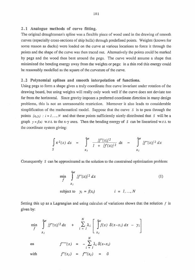
2. 2 Polynomial splines and smooth interpolation of functions. Using pegs to form a shape gives a truly coordinate free curve invariant under rotation of the

drawing board, but using weights will really only work well if the curve does not deviate too

far from the horizontal. Since gravity imposes a preferred coordinate direction in many design

problems, this is not an unreasonable restriction. Moreover it also leads to considerable

simplification of the mathematical model. Suppose that the curve S is to pass through the

points {x;,yJ : i = 1, ... , N and that these points sufficiently nicely distributed that S will be a

graph y = j(x) w.r.t. to the x-y axes. Then the bending energy of S can be linearized w.r.t. to

the coordinate system giving:

J ~e 2 (s) ds

s = r /f'(x)/2 dx

1 + /f'(x)/ 2 r /f"(x)/ 2 dx

Consequently s can be approximated as the solution to the constrained optimization problem:

rnr r /f"(x)f2 dx (1)

XJ

subject to Yi = f(xi) i = 1, ... ,N

Setting this up as a Lagrangian and using calculus of variations shows that the solution f is

given by:

rn;n r /f'(x)f2 dx

XJ

+ .~/· [ rf(x) ii(x-x;) dx - Yil

N

<=> f""(x) = l Aj O(X-Xj) i = 1

with

182

0

Yi

Thus f must be a cubic within each interval (x1,xi+I) and must be C 2 on the whole interval

[x1.xN1. More generally, given a set of points x1 i = 1, ... , N, a polynomial spline f(x) of degree

m and smoothness k is a function that is a polynomial of degree m in each subinterval (x1,xi+1)

and is of order c• over the whole interval. The points x1 are termed knot points. If in

addition, f(x) is a spline of order 2m+l, smoothness m and is chosen to minimize IJJ!"'i(x)/ 2 dx

subject to f(xi) = Yi at the knot points, then f is termed a natural spline. [3] is the standard

reference on polynomial splines, [11] describes splines in more general settings.

The most convenient formulation for determining f uses a basis of B-splines. A B-spline is a

generic polynomial spline with finite support; in particular the cubic B-spline associated with

the generic knot points { -2, -1, o, 1, 2) is:

r2)' -2 S X S -J

(x+2) 3 - (x+1)3 -J S X S 0 B(x) = (2-x)3 (1-x)3 0 S X S J

(2-x) 3 ] :f> X S 2

Simple rescaling will map this generic spline to the cubic B-spline B;(x) on any set of 5 knot

points {x1_2, x;_1 x1, x1+l> x1+:d· Now expanding f as:

N

f(x) 'I.aiBb) i = 1

gives a simple linear system Ba = y for the coefficients a,. The matrix B has entries B,1 = B;(x1), so its only non-zero elements are on the main diagonal and its two off-diagonals, so the

system can be rapidly solved in O(N) operations. Moreover a complete stability analysis can be

done that shows that the inversion is in general well-conditioned.

Error analysis for natural splines is fairly straightforward; the main result is that if g "' C2m+2

and f is the natural spline of order 2m+l interpolating g at N knots, then:

jjg(k)_ j(k)//oo ~ C h2m+2-kjjg(2m+2)//oo

where h = max /x,-x,_1j, and c is a constant independent of h and g.

Cubic splines have been extremely successful in many applications involving approximation of

functions, interpolation of time series and suchlike. In particular, as well as being accurate,

183

easily computed and easily interpreted, they are visually satisfying; it appears that the eye can

detect discontinuities in the first or second derivatives of a function of a single variable, but that

a C2 or better function appears smooth. These successes set up the benchmarks that smooth

interpolants of general curves are judged against, and have motivated the extensions of cubic

splines to curve fitting that will be discussed later.

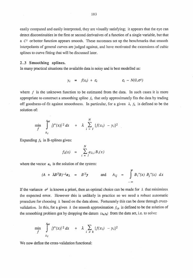
2. 3 Smoothing splines. In many practical situations the available data is noisy and is best modelled as:

where f is the unknown function to be estimated from the data. In such cases it is more

appropriate to construct a smoothing spline h. that only approximately fits the data by trading

off goodness-of-fit against smoothness. In particular, for a given A, !:~. is defined to be the

solution of:

m;n r /f'(x)/ 2 dx

XJ

Expanding fl in B-splines gives:

N

+ It L [f(x;) - YiF i = 1

N

f;,.(x) L a:J.,iBb) i = 1

where the vector a._ is the solution of the system:

J B /'(x) B/'(x) dx

If the variance u2 is known a priori, then an optimal choice can be made for A that minimizes

the expected error. However this is unlikely in practice so we need a robust automatic

procedure for choosing It based on the data alone. Fortunately this can be done through cross­

validation. In ti.is, for a given It the smooth approximation h .. • is defined to be the solution of

the smoothing problem got by dropping the datum (xk·YJ from the data set, i.e. to solve:

mjn r /f'(x)/ 2 dx

XJ

We now define the cross-validation functional:

184

N

V(A-) L Wk [h.k(Xk) - Yk)2 k = 1

V(?..) essentially measures how good a particular A. is in predicting missing data values. The

choice of the optimal A.* is then the minimizer of V(A.). It can be shown that this A.* is

asymptotically optimal in that as N r = it tends to the A. that would be chosen if the variance

was known. Moreover under certain reasonable choices for the weights w< it can be shown

([5], see also [6, 11]) that V(A) need not be calculated by constructing h .. ix<) separately for

each k, but can be expressed in terms of A., y and the generalized eigenvalues A; of the

system Ax; = A; B TBx;.

Again spline smoothing with the use of cross validation for estimation of the smoothing

parameter has worked very well in a wide range of practical problems, and so one would hope

that it could be included within the framework of a general variational construction for fitting

arbitrary smooth curves through noisy data.

2. 4 Parametric splines for interpolating curves in two or more dimensions. The success of splines in interpolating functions has made them the basis for a number of

constructions for interpolating arbitrary smooth curves in higher dimensions. These

constructions, however, are all based on a parametric representation of the curve followed by a

spline interpolation of each coordinate as a function of the parameter. As there appears to be no

natural variational form associated with any of these representations, the justification for using

any particular representation has to fall back on less intuitively satisfying reasons such as ease

of use.

In order to define these splines we use the following notation. x; = x{u;) = {xlu;), ... , xa(u,)}

will denote points on a curve in d dimensions parameterized by the variable u with knot points

at u;, i = 1, ... , N. A description of all these splines can be found in [4], but see also [9] for

details on NURBS and [1] for details on P-splines.

Bezier splines

In these the interpolating spline is represented as:

N

x(u) L ai B f (u) i = 1

where B~(u)

are the Bernstein polynomials. The a; are termed the control points. Bezier splines are

perhaps the oldest of the various splines used to approximate arbitrary curves and are the basis

of many smoothing routines in interactive drawing packages such as MacDraw. Note that the

185

curve interpolates the first and last control points, so a1 = x1 and aN= xN but the remainder of

the control points must be found by solving a dense system of equations, whose conditioning

will depend both on the data x1 and on the distribution of knots u1• For this reason individual

Bezier splines are often restricted to a low degree, and large curves are interpolated by patching

together several splines. Continuity of the curve's tangent vector across patches can be

enforced by noting that the direction of the tangent at an endpoint (say x1) lies along the line x2

- x1• Note also that x(u) always lies in the convex hull of the control points a;, a property that

also holds true for parametric B-splines and NURBS.

Parametric B-splines

In these the interpolating spline is represented as:

N

x(u) L aiB/u) i = 1

where the B;(u) are the B-splines defined above.

Non-Uniform Rational B-Splines (.NlJRBS}

In these the interpolating spline is represented as:

x(u)

N

La; w;B;(u) i = 1

N

Lw,B i = 1

where the B;(u) are again B-splines (almost always cubic splines). In addition to the properties

noted above NURBS have some additional virtu.es. First, since conics can be parameterized by

rational quadratics, NURBS can represent conic sections exactly. Second NURBS are

invariant under affine and projective transformations. In particular, for affine transformations

X --7 Ax+b:

Ax(u) + b

N

L (Aai +b) w;B;(u) i = 1

N

L w1B;(u) i = 1

For perspective transformations, let x ---- n(x) denote the projection through a viewpoint c on

to a plane that passes through the point p and has normal n. Then

n(x) = (1- a)x + ac where a (x-p) en (x-c) •n

and n(x(u)) =

186

N

L n(ai) wiBi(u) i = 1

N

L W;Bi(u) i = 1

This result is very useful in graphics displays since any 3D curve must be ftrst projected onto

the screen before it can be displayed. Thus a representation which is invariant under such

transformations can be used for both 2D lind 3D curve fitting without need for re-expression

when changing views.

a-splines

~-splines were introduced to take advantage of the fact that geometric smoothness (e.g.

continuity of the tangent vector and curvature) of a parameterized curve is a weaker requirement

than parametric smoothness (e.g. C2 continuity of the coordinates w.r.t. to u). In particular,

starting with a parameterized cubic B-spline representation, and relaxing the condition of

parametric smoothness to require only geometric smoothness frees up two parameters which

can then be adjusted to meet other objectives. The resultant curve is written as

N

x(u) · = L ai f]lu : /h/h) i = 1

where /31 controls the bias of the spline towards either endpoint and f32 controls the tension

(i.e. if f32 = 0 then the spline is an ordinary B-spline, while if /32 = oo the spline consists of

straight line segments).

2. 5 Strengths and weaknesses of interpolatory splines. The main advantage of interpolatory splines for curve fitting is that the underlying theory is

linear. The main disadvantage is that the basic theory of natural splines is derived in the context

of approximating functions. The advantages of a linear theory are simple algorithms for curve

fitting whose performance can be exhaustively analysed. The disadvantage is a setting that is

not invariant w.r.t. coordinate rotation, and so many results do not carry through to the fttting

of arbitrary curves. We now briefly list some of the consequences of this.

First, a non-invariant setting means that natural polynomial splines do not necessarily preserve

many important geometric properties such as convexity. Moreover they will suffer from

instability when approximating functions with infmite derivatives even if the function graphs

are well behaved when viewed simply as cur\res in the plane. The following example shows a

typical example of these problems: a cubic spline is used to approximate log x and the

approximation becomes increasingly oscillatory near the <>rigin.

187

/ "···· .• , ...... ,. l' ..... ,,.J/1,.1,,-;

I 1 I I l \ l Interpolating spline

~ .. ./

.. ~

Nevertheless, viewed as a curve in the plane, log x is a very well behaved convex curve and

one would expect that a "true" interpolatory spline got by minimizing curvature would also be

convex, and also be a very accurate approximation.

Second, the lack of an invariant variational formulation means that many useful results on

function approximation by splines do not apply when approximating curves by parametric

splines. In particular, any result depends crucially on the parameterization, and there seems to

be no optimal way to specify this from the data (although an algorithm is given in [9] for

determining knot points for NURBS that at least guarantees that the associated matrix B of

spline values is totally positive definite and so can be inverted using Gaussian elimination

without pivoting). I know of no results, for instance, on approximation of curves by

parametric splines that parallel the error bounds on approximation of functions by natural

splines. In practice most interpolation by parametric splines is done locally, so that the control

points ai are determined only by a few nearby x;. This is necessarily done on essentially ad

hoc basis. The same comments also apply to smoothing by parametric splines.

3 . Interpolation of curves by splines minimizing curvature.

Given the drawbacks of existing methods of curve fitting, we could try and define smooth

interpolants by a more exact model of the original draughtsman's spline. In particular, given

data {x; =(xi.YJ : i = 1 •...• N} we seek to fit a curve S through the data points that minimizes:

J IC2(s) ds

s (where s denotes arc length) and to explore the properties of the solution.

188

3. 1 Formal solution to the variational problem.

The minimization can be solved using much the same approach as for the linear case. In

particular, we flrst parameterize the curve S = {x(s) : 0 = s1 s s s sNJ by arc length, and switch

to intrinsic coordinates ( rp( s), s) where (/!( s) denotes the inclination of the curve to the horizontal

at the distance s along the curve. Since K2(s) = fql(s)j2, we have that the problem can be re­

formulated as: minimize over knot points s; and angular functions q; the expression:

subject to:

r /<p'(s)/ 2 ds

S· 1 r x'(s) ds Sr· 1 ~COS ({J(S)J dS Lsin <p(s)

Xi+l - X;

Fonning a Lagrangian as before by introducing the Lagrange multipliers A.; = p; (cos 'If;, sin 'If;)

and solving the Euler equations shows that q; must satisfy:

-p; sin (qy(s)- ljli)

subject to 0

and appropriate continuity conditions at the knots. An exact solution can be found for cp in

tenns of elliptic functions with two free parameters; this then leaves a system of nonlinear

equations to be solved for these parameters plus the knots si and the multipliers A.i.

3. 2 Problems with the formal solution.

There are a number of theoretical problems with this minimization as well as the obvious

practical problem of having to solve a fairly large nonlinear system of equations. First, there is

no guarantee that a solution even exists. The reason for this is that it is always possible to

reduce the value of the functional by appropriately lengthening the curve. To see why this is

possible, consider a very large circle of radius R. Then the length of this is 2nR and its

curvature is 1 !R, so the value of the functional is 2rc!R which can always be reduced by

increasing R. Thus even if a local minimum of finite length has been found, a lower cost

solution can be produced by taking out a segment of this curve between any two knot points

and replacing it by a very large loop.

Second, the splines produced by the formal solution are not always intuitively satisfying. For

example, Lee and Forsythe [7] show that the local minimizer of square curvature interpolating

points on a circle is not necessarily the circle.

189

3. 3 Alternative approaches and ltmreso!ved issues. The difficulties mentioned above mean that curvature minimizing splines are not widely used.

A survey of algorithms for their construction are given in [8], while [2] presents an algorithm

for constructing approximations based on spiral splines, in which the curvature is constrained

to vary only linearly between data points. An even simpler algorithm can be derived based on

approximation by arcs of circles; while this cannot be geometrically smooth, it has the

advantages of being simple to calculate and of being composed of objects that are standard

subroutines in many graphics systems.

The problem of non-existence of global minimizers may be due to an incorrect formulation;

perhaps with an alternative choice of curvature functional a global minimum may exist.

Likewise it may be possible to prove error bounds for smooth interpolants minimizing certain

curvature functionals; or that particular geometric properties (such as convexity or circularity of

the point data) are preserved by the interpolant; or that the functional form of the curve is

preserved under perspective projection. Finally it would be very useful to find a fommlation

that allowed the rigourous derivation of smoothing curves for noisy data along the lines of the

results for smoothing splines. These sort of results, however, appear to require the skills and

insights of a specialist variational geometer. Nevertheless, if a consistent theory could be

developed that established at least some of them, there would be considerable interest among

numerical analysts and computer graphics specialists in actually constructing the interpolants the

theory described.

4. Interpolation of surfaces.

We now look briefly at interpolation of surfaces and higher dimensional objects. Again there is

a fairly comprehensive linear theory of interpolating splines for smooth graphs, but in contrast

there seems to have been no practical work at all on constructing interpolating surfaces that

minimize some general function of curvature. In many ways this is an even more pressing

problem than construction of smooth curves, as the increase in full 3D graphics modelling,

especially in CAD (computer aided design), has required the construction of very large smooth

surfaces and therefore placed a premium on efficient representation. Moreover, as in many

CAD models these surfaces are often used to actually define an object, these representations

must also be invariant under rotation and suchlike transformations if they are to define the same

object under different views.

To bring this point home, let us roughly estimate the number ofpar<Lmeters needed to accurately

represent an smooth surface. I am aware of no useful results on the approximation of arbitrary

surfaces, but consider instead the simpler problem of approximating a smooth function f : 5Jid

190

-+ 9r from an approximation space sh ~:;; CF-1 where h represents some measure of resolution.

Then typically sh will have dimension N- O(h-<~). Moreover the best approximation PI to f

in Sh will be in error by Iff- P/1/ - O(hP), so that in order to ensure that Iff- P/1/ ~e we will

have to choose Sh to be sufficiently large that its dimension satisfies:

N O((plh)d) O((pfeliP )d)

Thus by upping the order of the approximation we can substantially reduce the size of the

approximation needed to accurately represent the function. This is of special importance when

we consider that while display of the approximation takes only O(N) operations, many other

important tasks, such as finding a CAD object represented as a surface in a database of such

objects may take O(N2) operations, or even more.

4 .1 Thin plate splines. The natural extension of Eq. (1) for defining a smooth interpolant to surface data is:

m;n J /f:xx(x,y)j2 + 2 /fxy(x,y)/ 2 + //yy(x,y)/ 2 dx dy

9(;;>2

subject to Zi = f(xi,Yi) i = 1, ... ,N

Letting x denote the point (x,y), calculus of variations establishes that:

!l 2f(x)

with

N

- L. Ai O(X-Xi) i = 1

Zi

plus the condition that f(x) asymptote to a hyperplane as fx/ i oo. Therefore

N

f(x) L ai cp(fx-xJ) + ao + a_1X + iN 1

where 0 L ai i = 1

and cp(r) = r2[nr

a_zy

The resulting splines are known as thin plate splines as the physical analogue of this procedure

(corresponding to a draughtsman's use of a spline to interpolate a curve) is to load a thin metal

plate with weights at the locations x; and so force it to take on heights z;. Thin plate splines

have been successfully used in a number of applications [11], and can be generalized to

191

interpolate surfaces in higher dimensions or with smoother functions; the basic spline derived

by minimizing derivatives of order m in d dimensions is:

qJ(r) v2m-d ln r Lr2m-d

d even

d odd

Extensions to the case of smoothing splines are straight-forward; Dr. M. Hutchinson of CRES

at ANU has a FORTRAN package that uses cross validation to fit smooth thin plate splines

through arbitrary data sets.

4. 2 Surface patches. Unlike B-splines, thin plate splines do not form the basis for any surface constructions in

computer graphics. The main reason for this is that they have infinite support and so are not

suitable for modelling essentially localized surfaces and cannot be easily modified. Instead

most surface modelling in computer graphics is done using quadrilateral patches formed by

taking tensor products of the parametric splines described in section 3. A typical patch

composed of B-splines would be:

x(u,v)

M N

L L au B ;(u) Bj(v) i=lj=l

where the a;j are now control points in 913 and the patch is defined over a grid of knots

formed by taking the product of the two knot vectors for u and v respectively.

The patches themselves are usually C2 or better, but it is difficult to ensure better than C 1

continuity when joining two patches. This is actually not a major problem as it when it comes

to surfaces, it seems that a surface is visually smooth simply as long as its tangent plane is

continuous. Moreover this geometric continuity is even weaker than the C 1 parametric

continuity achieved by most patch joins. Patches run into difficulty, however, when fitting data

that can not be arranged onto an essentially rectangular grid of knot points; while the odd

irregular element within a grid can be coped with, truly irregular grids present very messy

problems. More generally, surface fitting by patches is an involved and intricate discipline,

albeit one of great importance (see [9, 10] for further details),

':L 3 Variational problems in surface fitting. As already noted there appears to be no available results on characterization or calculation of

smooth interpolants that minimize curvature measures. There is some reason to believe that

these interpolants may differ significantly from the thin plate splines described in section 4.1;

the singularities at the origin (and therefore at data points) exhibited by thin plate splines may

not be the same as those of true curvature minimizing interpolants at data points. Nevertheless

192

both the general shape of such interpolants and any properties they may have is still obscure,

and equally importantly there is no obvious way of actually calculating them.

There are a number of other important variational problems in surface modelling by patches. In

particular a surface defined by a very large and possibly irregular grid of patches often needs to

be systematically re-gridded to produce a smaller, more regular but essentially equally accurate

representation. This problem arises very commonly in CAD surfaces constructed from

measuring real world shapes. Data may be collected, for example, by shining a finely spaced,

regular grid of bright lights onto the surface and then measuring the resultant distortion of the

grid in an image of the surface: the distortion gives the depth of the surface in the direction of

view. This and similar methods have two problems: they tend to heavily over-sample smooth

regions of the object; and they produce very irregular grids in areas where the object's local

topology is definitely not a graph (e.g. where the handle of a cup joins its body).

If the surface is topologically equivalent to a disk, one possible solution is to find a conformal

mapping 'J of the surface onto the unit disk (or square). Next a uniform grid can be placed on

the disk and then mapped back to the surface by ;r-1• The resulting grid on the surface will

also be regular and so suitable for patch construction. Moreover the surface grid should be

concentrated in regions of high curvature, but spread out in smoother regions. Conformal

maps can be constructed as the minima of certain curvature functionals; the question is whether

these are the most suitable variational forms for this particular problem.

5 . Summary of open questions.

In conclusion, it seems that the following questions are still open. Positive answers to them

would be not only of considerable theoretical interest in extending existing results for the linear

theory of approximating smooth graphs to the approximation of smooth curves, but also of

great practical import for computer graphics. The theoretical questions are:

1 . Is there a natural variational formulation for defining a smooth curve I surface to interpolate arbitrar; data in two or more dimensions?

2. Can the solutions to such formulations be characterized?

3. Do the solutions preserve general geometric properties such as convexity?

4. Can useful error bounds be derived for the approximation of smooth curves I surfaces?

5 . Can the formulations be extended to define smoothing curves I surfaces for noisy data, and do these have same form as the exact interpolants? Can smoothing be done robustly and automatically?

193

6. Is the general functional form of the interpolants invariant under perspective transformations?

The more practical questions are:

7. What is the "best" set of graphics primitives for generating curves and surfaces in software and hardware?

8. Can the solutions be efficiently computed?

Finally, in regard to the last question, the nonlinear nature of the problems means that iterative

methods are likely to be used for their solution. Consider the general problem:

min V(S) s

Jl(K(s)) ds

s subject to various constraints

where I(K) is some function of curvature. Direct application of steepest descent would give

(constrained) iterates of the form:

This looks very similar to general surface flow problems of the form:

d~~t) - VV(S(t))

that have been widely studied by variational geometers, so that it may be possible to use

existing results both to prove existence of solutions and convergence of numerical algorithms to

them. Furthermore, higher order iterative algorithms such as Newton's method:

where Hv is the Hessian, can also be translated into surface flow problems of the form:

dS(t) dt

-{Hv(S(t))]-1 VV(S(t))

In the light of the many extra stability and convergence properties that Newton's method has in

comparison with steepest descent, it is interesting to speculate what extra convergence

properties the above surface flow may have.

194

Acknowledgements.

I would like to thank Ian Coope for some very helpful pointers and references on the problem

of finding the interpolant with minimum square curvature, and the Centre and DITAC for the

opportunity and support to attend the conference.

References

[1] R. Bartels, J. Beatty and B. Barsky, An Introduction to Splines for Use in Computer Graphics and Geometric Modelling, Morgan Kaufman, Los Altos, California, 1987.

[2] I. Coope, Curve fitting with nonlinear spiral splines, preprint, 1991.

[3] C. de Boor, A Practical Guide to Splines, Springer-Verlag, New York, 1978.

[4] J.D. Foley, A. van Dam, S.K. Feiner and J.F. Hughes, Computer Graphics: Principles and Practice, Addison-Wesley, Reading, Massachussetts, 1990.

[5] G. Golub, M. Heath and G. Wahba, Generalized cross validation as a method for choosing a good ridge parameter, Technometrics, 21 (1979), 215-24.

[6] M. Hutchinson and F. de Hoog, Smoothing noisy data with spline functions, Numer. Math., 47 (1985), 99-106.

[7] E.H. Lee and G.E. Forsythe, Variational study of nonlinear spline curves, SIAM Rev., 15 (1973), 120-33.

[8] M.A. Malcolm, On the computation of nonlinear spline functions, SIAM J. Numer. Anal., 14 (1977), 254-82.

[9] L. Piegl, On NURBS: A summary, IEEE Comp. Graphics & Applies., (1991), 55-71.

[10] R.F. Sarraga, Computer modelling of surfaces with arbitrary shapes, IEEE Graphics & Applies., (1990), 67-77.

[11] G.Wahba, Spline Models for Observational Data, SIAM, Philadelphia, 1990.

Information Technology Division, Electronics Research Laboratory, DSTO, P.O. Box 1600, Salisbury, S.A. 5108, Australia.