some topics in computational topology - duke universitysayan/jmm/computational.pdf · some topics...

Some Topics in Computational

Topology

Yusu Wang

Ohio State University

AMS Short Course 2014

Introduction

Much recent developments in computational topology

Both in theory and in their applications

E.g, the theory of persistence homology

[Edelsbrunner, Letscher, Zomorodian, DCG 2002], [Zomorodian and

Carlsson, DCG 2005], [Carlsson and de Silva, FoCM 2010], …

This short course:

A computational perspective:

Estimation and inference of topological information / structure from

point clouds data

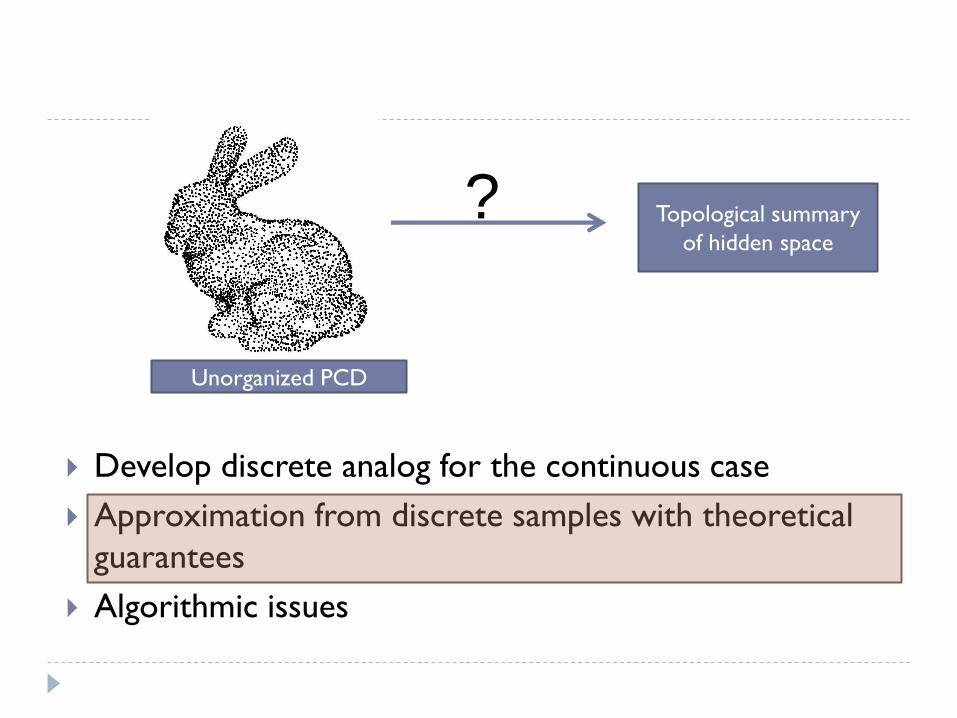
Develop discrete analog for the continuous case

Approximation from discrete samples with theoretical

guarantees

Algorithmic issues

Topological summary

of hidden space

?

Unorganized PCD

Main Topics

From PCDs to simplicial complexes

Sampling conditions

Topological inferences

Outline


Delaunay, Cech, Vietoris-Rips, witness complexes

Graph induced complex

Sampling conditions

Local feature size, and homological feature size

Topology inference

Homology inference

Handling noise

Approximating cycles of shortest basis of the first homology group

Approximating Reeb graph

From PCD to Simplicial Complexes

Choice of Simplicial Complexes

to build on top of point cloud data

Delaunay Complex

Given a set of points 𝑃 = 𝑝1, 𝑝2, … , 𝑝𝑛 ⊂ 𝑅𝑑

Delaunay complex 𝐷𝑒𝑙 𝑃 A simplex 𝜎 = {𝑝𝑖0 , 𝑝𝑖1 , … , 𝑝𝑖𝑘 } is in 𝐷𝑒𝑙 𝑃 if and only if

There exists a ball 𝐵 whose boundary contains vertices of 𝜎, and that

the interior of 𝐵 contains no other point from 𝑃.

Delaunay Complex

Many beautiful properties

Connection to Voronoi diagram

Foundation for surface reconstruction and meshing in 3D [Dey, Curve and Surface Reconstruction, 2006],

[Cheng, Dey and Shewchuk, Delaunay Mesh Generation, 2012]

However,

Computationally very expensive in high dimensions

Čech Complex


Given a real value 𝑟 > 0, the Čech complex 𝐶𝑟 𝑃 is the nerve

of the set 𝐵 𝑝𝑖 , 𝑟 𝑖∈ 1,𝑛

where 𝐵𝑟 𝑝𝑖 = 𝐵 𝑝𝑖 , 𝑟 = { 𝑥 ∈ 𝑅𝑑 ∣ 𝑑 𝑝𝑖 , 𝑥 < 𝑟 }

I.e, a simplex 𝜎 = {𝑝𝑖0 , 𝑝𝑖1 , … , 𝑝𝑖𝑘 } is in 𝐶𝑟 𝑃 if

𝐵𝑟 𝑝𝑖𝑗0≤𝑗≤𝑘 ≠ Φ.

The definition can be extended to a finite sample 𝑃 of a metric

space.

Rips Complex


Given a real value 𝑟 > 0, the Vietoris-Rips (Rips) complex

𝑅𝑟 𝑃 is:

{ 𝑝𝑖0 , 𝑝𝑖1 , … , 𝑝𝑖𝑘 ∣ 𝐵𝑟 𝑝𝑖𝑙 ∩ 𝐵𝑟 𝑝𝑖𝑗 ≠ ∅,∀ 𝑙, 𝑗 ∈ [0, 𝑘 ]}.

Rips and Čech Complexes

Relation in general metric spaces

𝐶𝑟 𝑃 ⊆ 𝑅𝑟 𝑃 ⊆ 𝐶2𝑟 𝑃

Bounds better in Euclidean space

Simple to compute

Able to capture geometry and topology

We will make it precise shortly

One of the most popular choices for topology inference in recent

years

However:

Huge sizes

Computation also costly

Witness Complexes

A simplex 𝜎 = 𝑞0, … , 𝑞𝑘 is weakly witnessed by a point x if

𝑑 𝑞𝑖 , 𝑥 ≤ 𝑑 𝑞, 𝑥 for any 𝑖 ∈ 0, 𝑘 and 𝑞 ∈ 𝑄 ∖ {𝑞0, … , 𝑞𝑘}.

is strongly witnessed if in addition 𝑑 𝑞𝑖 , 𝑥 = 𝑑 𝑞𝑗 , 𝑥 , ∀𝑖, 𝑗 ∈ 0, 𝑘

Given a set of points 𝑃 = 𝑝1, 𝑝2, … , 𝑝𝑛 ⊂ 𝑅𝑑 and a subset

𝑄 ⊆ 𝑃 ,

The witness complex 𝑊 𝑄,𝑃 is the collection of simplices with

vertices from 𝑄 whose all subsimplices are weakly witnessed by a

point in 𝑃.

[de Silva and Carlsson, 2004] [de Silva 2003]

Can be defined for a general metric space

𝑃 does not have to be a finite subset of points

Intuition

𝐿: landmarks from 𝑃, a way to subsample.

𝑃 𝐿 ⊆ 𝑃 𝑊(𝐿, 𝑃)

Witness Complexes

Greatly reduce size of complex

Similar to Delaunay triangulation, remove redundancy

Relation to Delaunay complex

𝑊 𝑄,𝑃 ⊆ 𝐷𝑒𝑙 𝑄 if 𝑄 ⊆ 𝑃 ⊂ 𝑅𝑑

𝑊 𝑄,𝑅𝑑 = 𝐷𝑒𝑙 𝑄

𝑊 𝑄,𝑀 = 𝐷𝑒𝑙 𝑀 𝑄 if 𝑀 ⊆ 𝑅𝑑 is a smooth 1- or 2-manifold

[Attali et al, 2007]

However,

Does not capture full topology easily for high-dimensional

manifolds

Remark

Rips complex

Capture homology when input points are sampled dense

enough

But too large in size

Witness complex

Use a subsampling idea

Reduce size tremendously

May not be easy to capture topology in high-dimensions

Combine the two ?


[Dey, Fan, Wang, SoCG 2013]

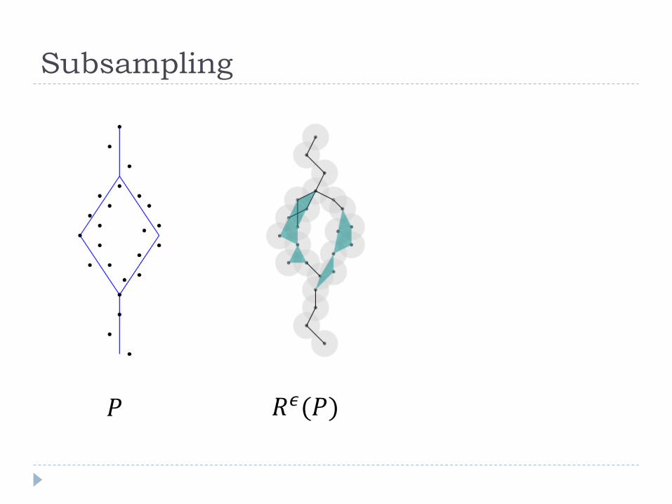
Subsampling

𝑃 𝑅𝜖(𝑃)

Subsampling -cont

𝑃 𝑄 ⊆ 𝑃 𝑅𝑟 𝑄 𝑊(𝑄, 𝑃)

𝑄 ⊆ 𝑃 𝑅𝑟 𝑄 𝑊(𝑄, 𝑃)

Subsampling -cont

Subsampling - cont

𝑅𝜖(𝑃) 𝑊(𝑄, 𝑃) 𝒢𝑟(𝑄, 𝑃)

Graph Induced Complex

[Dey, Fan, Wang, SoCG 2013]

𝑃: finite set of points

(𝑃, 𝑑): metric space

𝐺(𝑃): a graph

𝑄 ⊂ 𝑃: a subset

𝜋 𝑝 : the closest point of

𝑝 ∈ 𝑃 in 𝑄


Graph induced complex 𝒢 𝑃, 𝑄, 𝑑 : 𝑞0, … , 𝑞𝑘 ⊆ 𝑄

if and only if there is a (k+1)-clique in 𝐺 𝑃 with vertices

𝑝0, … , 𝑝𝑘 such that 𝜋 𝑝𝑖 = 𝑞𝑖 , for any 𝑖 ∈ [0, 𝑘].

Similar to geodesic Delaunay [Oudot, Guibas, Gao, Wang, 2010]

Graph induced complex depends on the metric 𝑑:

Euclidean metric

Graph based distance 𝑑𝐺


Small size, but with homology inference guarantees

In particular:

𝐻1 inference from a lean sample


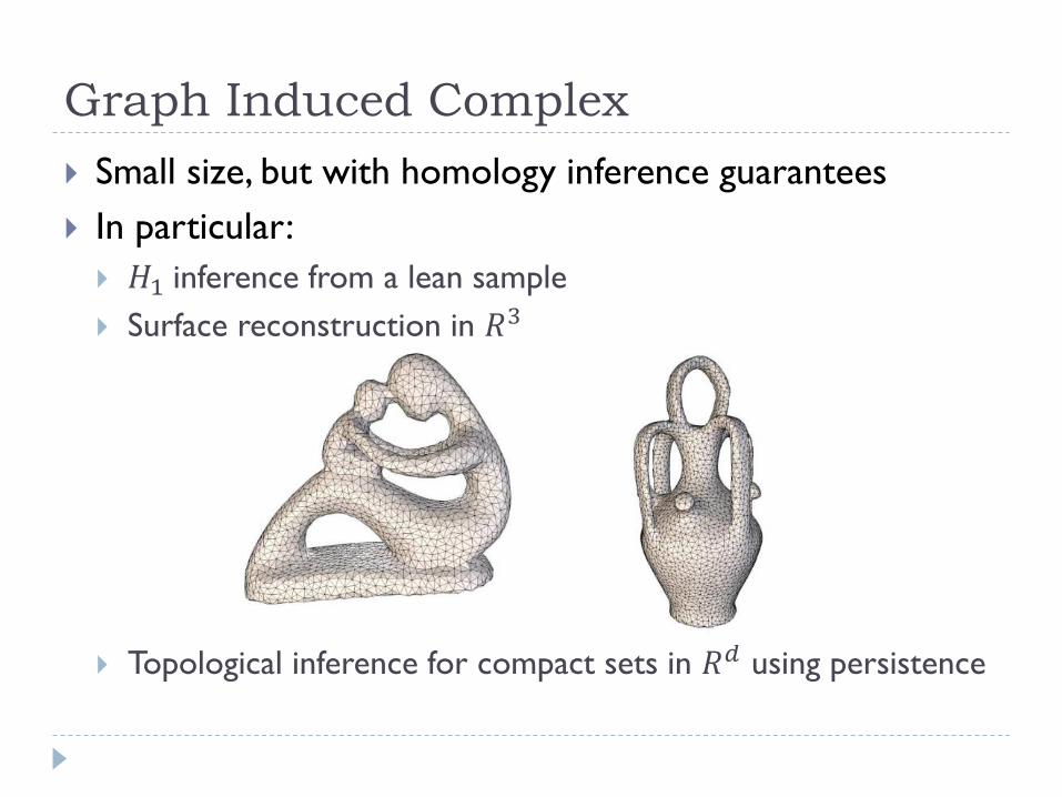
Small size, but with homology inference guarantees

In particular:

𝐻1 inference from a lean sample

Surface reconstruction in 𝑅3

Topological inference for compact sets in 𝑅𝑑 using persistence

Outline




Sampling conditions


Topology inference

Homology inference

Handling noise



Sampling Conditions

Motivation

Theoretical guarantees are usually obtained when input

points 𝑃 sampling the hidden domain “well enough”.

Need to quantify the “wellness”.

Two common ones based on:

Local feature size

Weak feature size

Distance Function

𝑋 ⊂ 𝑅𝑑: a compact subset of 𝑅𝑑

Distance function 𝑑𝑋: 𝑅𝑑 → 𝑅+ ∪ 0

𝑑𝑋 𝑥 = min𝑦∈𝑋

𝑑 𝑥, 𝑦

𝑑𝑋 is a 1-Lipschitz function

𝑋𝛼: 𝛼-offset of 𝑋

𝑋𝛼 = {𝑦 ∈ 𝑅𝑑 ∣ 𝑑 𝑦, 𝑋 ≤ 𝛼}

Given any point 𝑥 ∈ 𝑅𝑑 Γ 𝑥 ≔ { 𝑦 ∈ 𝑋 ∣ 𝑑 𝑥, 𝑦 = 𝑑𝑋 𝑥 }

Medial Axis

The medial axis Σ of 𝑋 is the closure of the set of points

𝑥 ∈ 𝑅𝑑 such that Γ 𝑥 ≥ 2

Γ 𝑥 ≥ 2 means that there is a medial ball 𝐵𝑟 𝑥 touching

𝑋 at more than 1 point and whose interior is empty of points

from 𝑋.

Courtesy of [Dey, 2006]

Local Feature Size

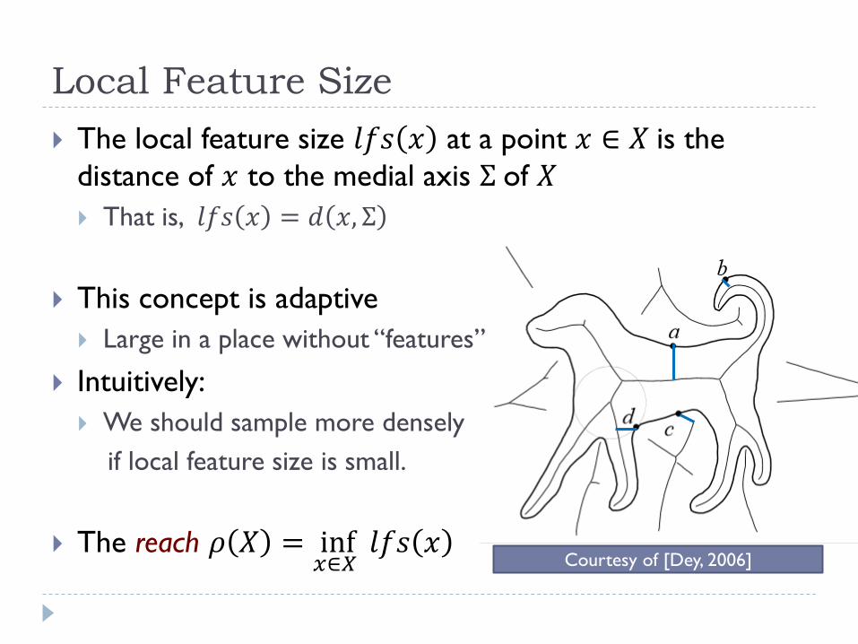
The local feature size 𝑙𝑓𝑠 𝑥 at a point 𝑥 ∈ 𝑋 is the

distance of 𝑥 to the medial axis Σ of 𝑋

That is, 𝑙𝑓𝑠 𝑥 = 𝑑 𝑥, Σ

This concept is adaptive

Large in a place without “features”

Intuitively:

We should sample more densely

if local feature size is small.

The reach 𝜌 𝑋 = inf𝑥∈𝑋 𝑙𝑓𝑠 𝑥

Courtesy of [Dey, 2006]

Gradient of Distance Function

Distance function not differentiable on the medial axis

Still can define a generalized concept of gradient

[Lieutier, 2004]

For 𝑥 ∈ 𝑅𝑑 ∖ 𝑋,

Let 𝑐𝑋 𝑥 and 𝑟𝑋 𝑥 be the center and radius of the smallest

enclosing ball of point(s) in Γ 𝑥

The generalized gradient of distance function

𝛻X 𝑥 = 𝑥 − 𝑐𝑋 𝑥

𝑟𝑋 𝑥

Flow lines induced by the generalized gradient

Examples:

Critical Points

A critical point of the distance function is a point whose

generalized gradient 𝛻𝑋 𝑥 vanishes

A critical point is either in 𝑋 or in its medial axis Σ

Weak Feature Size

Given a compact 𝑋 ⊂ 𝑅𝑑 , let 𝐶 ⊂ 𝑅𝑑 denote

the set of critical points of the distance function 𝑑𝑋 that are

not in 𝑋

Given a compact 𝑋 ⊂ 𝑅𝑑 , the weak feature size is

𝑤𝑓𝑠 𝑋 = inf𝑥∈X𝑑 𝑥, 𝐶

Equivalently,

𝑤𝑓𝑠 𝑋 is the infimum of the positive critical value of 𝑑𝑋

𝜌 𝑋 ≤ 𝑤𝑓𝑠 𝑋

Why Distance Field?

Theorem [Offset Homotopy] [Grove’93]

If 0 < 𝛼 < 𝛼′ are such that there is no critical value of 𝑑𝑋 in the

closed interval 𝛼, 𝛼′ , then 𝑋𝛼′ deformation retracts onto 𝑋𝛼 .

In particular, 𝐻 𝑋𝛼 ≅ 𝐻 𝑋𝛼′

.

Remarks:

For the case of compact set 𝑋, note that it is possible that 𝑋𝛼,

for sufficiently small 𝛼 > 0, may not be homotopy equivalent

to 𝑋0 = 𝑋.

Intuitively, by above theorem, we can approximate 𝐻 𝑋𝛼 for

any small positive 𝛼 from a thickened version (offset) of 𝑋𝛼.

The sampling condition makes sure that the discrete sample is

sufficient to recover the offset homology.

Typical Sampling Conditions

Hausdorff distance 𝑑𝐻 𝐴, 𝐵 between two sets 𝐴 and 𝐵

infinumum value 𝛼 such that 𝐴 ⊆ 𝐵𝛼 and 𝐵 ⊆ 𝐴𝛼

No noise version:

A set of points 𝑃 is an 𝜖-sample of 𝑋

if 𝑃 ⊂ 𝑋 and 𝑑𝐻 𝑃, 𝑋 ≤ 𝜖

With noise version:

A set of points 𝑃 is an 𝜖-sample of 𝑋 if 𝑑𝐻 𝑃, 𝑋 ≤ 𝜖

Theoretical guarantees will be achieved when 𝜖 is small

with respect to local feature size or weak feature size

Outline




Sampling conditions


Topology inference

Homology inference

Handling noise



Homology Inference from PCD

Problem Setup

A hidden compact 𝑋 (or a manifold 𝑀)

An 𝜖-sample 𝑃 of 𝑋

Recover homology of 𝑋 from some complex built on 𝑃

will focus on Čech complex and Rips complex

Union of Balls

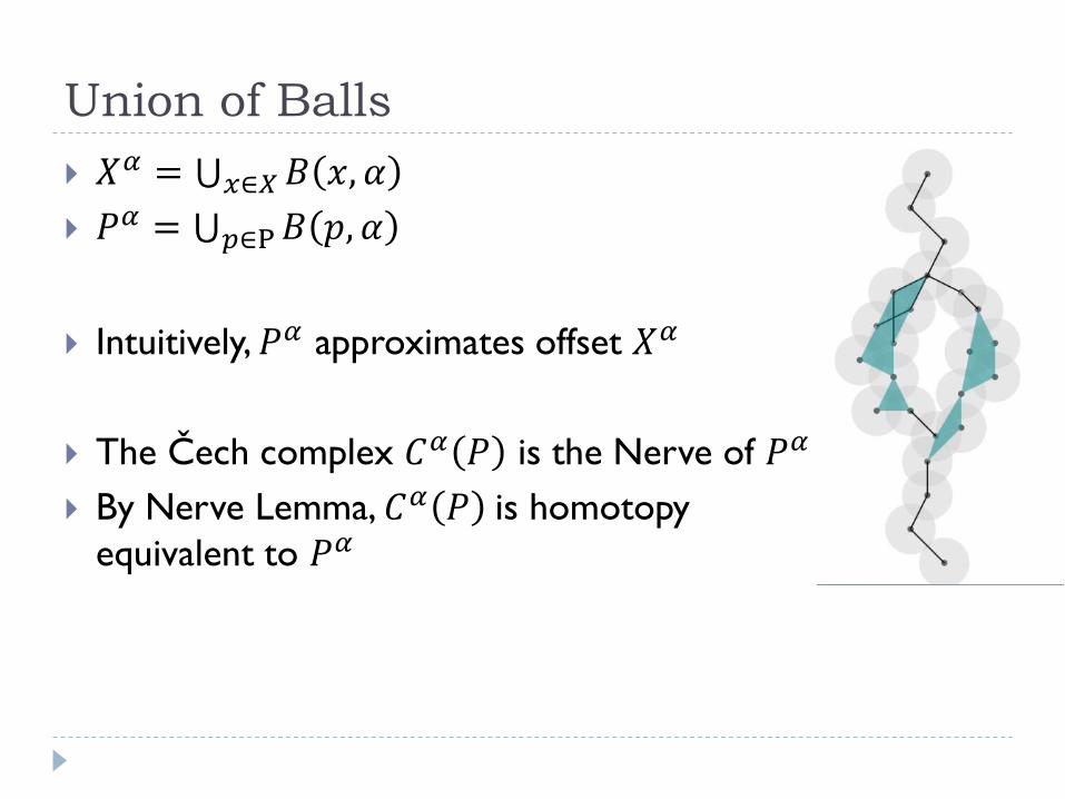
𝑋𝛼 = 𝐵 𝑥, 𝛼𝑥∈𝑋

𝑃𝛼 = 𝐵 𝑝, 𝛼𝑝∈P

Intuitively, 𝑃𝛼 approximates offset 𝑋𝛼

The Čech complex 𝐶𝛼 𝑃 is the Nerve of 𝑃𝛼

By Nerve Lemma, 𝐶𝛼 𝑃 is homotopy

equivalent to 𝑃𝛼

Smooth Manifold Case

Let 𝑋 be a smooth manifold embedded in 𝑅𝑑

Theorem [Niyogi, Smale, Weinberger]

Let 𝑃 ⊂ 𝑋 be such that 𝑑𝐻 𝑋, 𝑃 ≤ 𝜖. If 2𝜖 ≤ 𝛼 ≤3

5𝜌 𝑋 ,

there is a deformation retraction from 𝑃𝛼 to 𝑋.

Corollary A

Under the conditions above, we have H X ≅ 𝐻 𝑃𝛼 ≅ 𝐻 𝐶𝛼 𝑃 .

How about using Rips complex instead of Čech complex?

Recall that 𝐶𝑟 𝑃 ⊆ 𝑅𝑟 𝑃 ⊆ 𝐶2𝑟 𝑃

inducing

𝐻(𝐶𝑟) → 𝐻(𝑅𝑟) → 𝐻(𝐶2𝑟)

Idea [Chazal and Oudot 2008]:

Forming interleaving sequence of homomorphism to connect

them with the homology of the input manifold 𝑋 and its offsets

𝑋𝛼

Convert to Cech Complexes

Lemma A [Chazal and Oudot, 2008]:

The following diagram commutes:

𝐻 𝑃𝛼 𝐻 𝑃𝛽

𝐻 𝐶𝛼 𝐻 𝐶𝛽

𝑖∗

𝑖∗

ℎ∗ ℎ∗

Corollary B

Let 𝑃 ⊂ 𝑋 be s.t. 𝑑𝐻 𝑋, 𝑃 ≤ 𝜖. If 2𝜖 ≤ 𝛼 ≤ 𝛼′ ≤3

5𝜌 𝑋 ,

H X ≅ 𝐻 𝐶𝛼 ≅ 𝐻 𝐶𝛽 where the second isomorphism is

induced by inclusion.

From Rips Complex

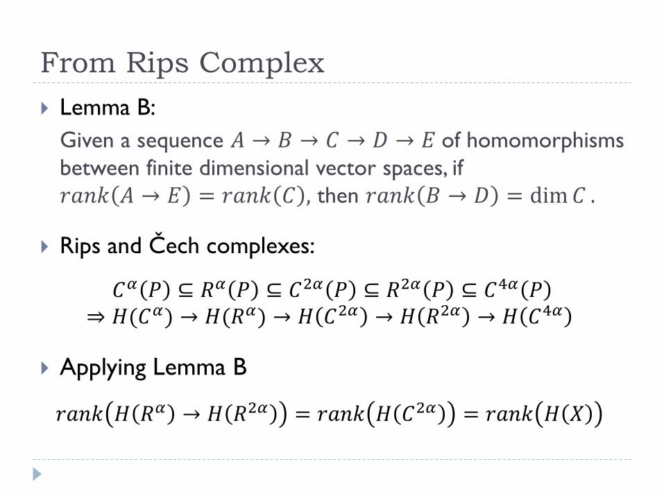
Lemma B:

Given a sequence 𝐴 → 𝐵 → 𝐶 → 𝐷 → 𝐸 of homomorphisms

between finite dimensional vector spaces, if

𝑟𝑎𝑛𝑘 𝐴 → 𝐸 = 𝑟𝑎𝑛𝑘 𝐶 , then 𝑟𝑎𝑛𝑘 𝐵 → 𝐷 = dim𝐶 .

Rips and Čech complexes:

𝐶𝛼 𝑃 ⊆ 𝑅𝛼 𝑃 ⊆ 𝐶2𝛼 𝑃 ⊆ 𝑅2𝛼 𝑃 ⊆ 𝐶4𝛼 𝑃

⇒ 𝐻(𝐶𝛼) → 𝐻(𝑅𝛼) → 𝐻 𝐶2𝛼 → 𝐻 𝑅2𝛼 → 𝐻 𝐶4𝛼

Applying Lemma B

𝑟𝑎𝑛𝑘 𝐻 𝑅𝛼 → 𝐻 𝑅2𝛼 = 𝑟𝑎𝑛𝑘 𝐻 𝐶2𝛼 = 𝑟𝑎𝑛𝑘 𝐻 𝑋

The Case of Compact

In contrast to Corollary A, now we have the following

(using Lemma B).

Lemma C [Chazal and Oudot 2008]:

Let 𝑃 ⊂ 𝑅𝑑 be a finite set such that 𝑑𝐻 𝑋, 𝑃 < 𝜖 for some

𝜖 <1

4𝑤𝑓𝑠 𝑋 . Then for all 𝛼, 𝛽 ∈ 𝜖, 𝑤𝑓𝑠 𝑋 − 𝜖 such

that 𝛽 − 𝛼 ≥ 2𝜖, and for all 𝜆 ∈ 0,𝑤𝑓𝑠 𝑋 , we have

𝐻 𝑋𝜆 ≅ 𝑖𝑚𝑎𝑔𝑒 𝑖∗ , where 𝑖∗: 𝐻 𝑃𝛼 → 𝐻 𝑃𝛽 is the

homomorphism between homology groups induced by the

canonical inclusion 𝑖: 𝑃𝛼 → 𝑃𝛽.

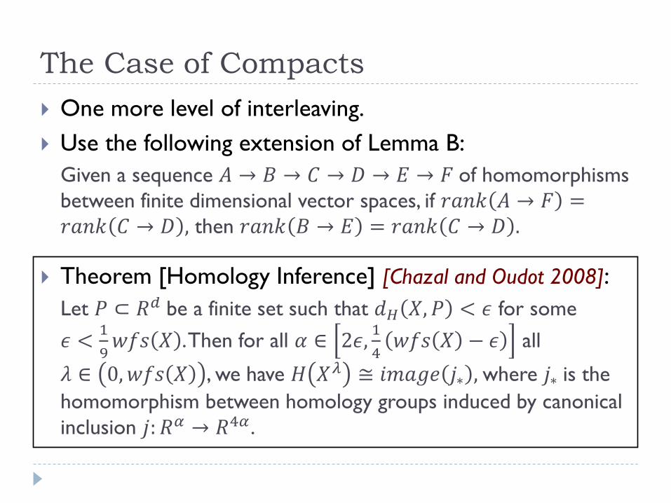
The Case of Compacts

One more level of interleaving.

Use the following extension of Lemma B:

Given a sequence 𝐴 → 𝐵 → 𝐶 → 𝐷 → 𝐸 → 𝐹 of homomorphisms

between finite dimensional vector spaces, if 𝑟𝑎𝑛𝑘 𝐴 → 𝐹 =𝑟𝑎𝑛𝑘 𝐶 → 𝐷 , then 𝑟𝑎𝑛𝑘 𝐵 → 𝐸 = 𝑟𝑎𝑛𝑘 𝐶 → 𝐷 .

Theorem [Homology Inference] [Chazal and Oudot 2008]:


𝜖 <1

9𝑤𝑓𝑠 𝑋 . Then for all 𝛼 ∈ 2𝜖,

1

4𝑤𝑓𝑠 𝑋 − 𝜖 all

𝜆 ∈ 0, 𝑤𝑓𝑠 𝑋 , we have 𝐻 𝑋𝜆 ≅ 𝑖𝑚𝑎𝑔𝑒 𝑗∗ , where 𝑗∗ is the

homomorphism between homology groups induced by canonical

inclusion 𝑗: 𝑅𝛼 → 𝑅4𝛼.

Theorem [Homology Inference] [Chazal and Oudot 2008]:


𝜖 <1

9𝑤𝑓𝑠 𝑋 . Then for all 𝛼 ∈ 2𝜖,

1

4𝑤𝑓𝑠 𝑋 − 𝜖 all 𝜆 ∈

0,𝑤𝑓𝑠 𝑋 , we have 𝐻 𝑋𝜆 ≅ 𝑖𝑚𝑎𝑔𝑒 𝑗∗ , where 𝑗∗ is the

homomorphism between homology groups induced by canonical

inclusion 𝑗: 𝑅𝛼 → 𝑅4𝛼.

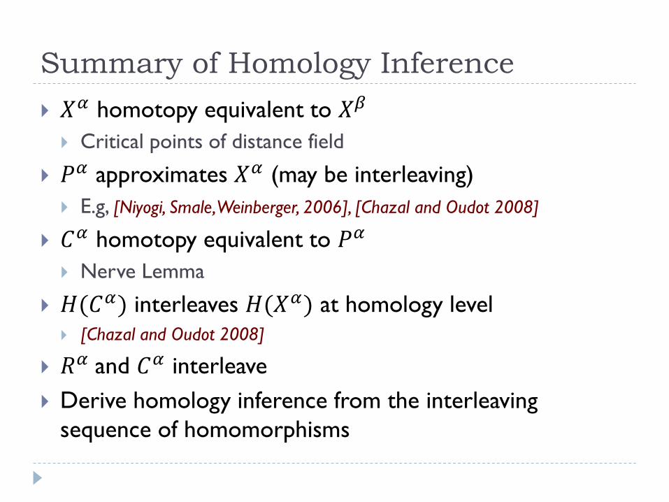
Summary of Homology Inference

𝑋𝛼 homotopy equivalent to 𝑋𝛽

Critical points of distance field

𝑃𝛼 approximates 𝑋𝛼 (may be interleaving)

E.g, [Niyogi, Smale, Weinberger, 2006], [Chazal and Oudot 2008]

𝐶𝛼 homotopy equivalent to 𝑃𝛼

Nerve Lemma

𝐻(𝐶𝛼) interleaves 𝐻(𝑋𝛼) at homology level

[Chazal and Oudot 2008]

𝑅𝛼 and 𝐶𝛼 interleave

Derive homology inference from the interleaving

sequence of homomorphisms

Outline




Sampling conditions


Topology inference

Homology inference

Handling noise



Handling of Noise

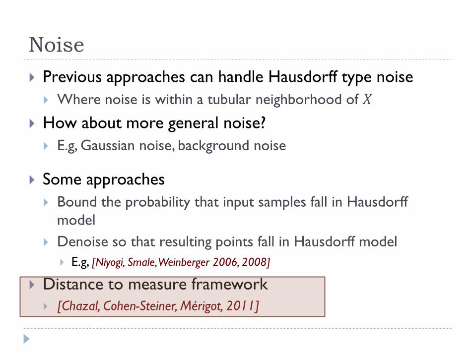
Noise

Previous approaches can handle Hausdorff type noise

Where noise is within a tubular neighborhood of 𝑋

How about more general noise?

E.g, Gaussian noise, background noise

Some approaches

Bound the probability that input samples fall in Hausdorff

model

Denoise so that resulting points fall in Hausdorff model

E.g, [Niyogi, Smale, Weinberger 2006, 2008]

Distance to measure framework

[Chazal, Cohen-Steiner, Mérigot, 2011]

Courtesy of Chazal et al 2011

Overview

Input:

A set of points 𝑃 sampled from a probabilistic measure 𝜇 on

𝑅𝑑 potentially concentrated on a hidden compact (e.g,

manifold) 𝑋.

Goal:

Approximate topological features of 𝑋

Main Idea

The work of [Chazal, Cohen-Steiner, Mérigot, 2011]

A new distance function 𝑑𝜇,𝑚 to a probability 𝜇 measure

(ie., distance to measures) to replace the role of distance

function 𝑑𝑋.

Show that the two distance fields are close (in 𝐿∞ norm)

Topological inference follows from some stability results

or the interleaving sequences

Definitions

𝜇: a probability measure on 𝑅𝑑 ; 𝜇 𝑅𝑑 = 1

0 < 𝑚,𝑚0 < 1: mass parameters

𝛿𝜇,𝑚: a pseudo-distance function such that

𝛿𝜇,𝑚 x ≔ inf{r > 0; 𝜇 𝐵 𝑥, 𝑟 > 𝑚 }

where 𝐵 𝑥, 𝑟 is the closed Euclidean ball at 𝑥

That is, 𝛿𝜇,𝑚 x is the radius of the ball necessary in

order to enclose mass 𝑚

Distance to measure 𝑑𝜇,𝑚0:

𝑑2𝜇,𝑚0 𝑥 =1

𝑚0 𝛿𝜇,𝑚 𝑥

2 𝑑𝑚𝑚0

0

Distance to Measures

Distance to measure 𝑑𝜇,𝑚0:

𝑑𝜇,𝑚02 𝑥 =

1

𝑚0 𝛿𝜇,𝑚 𝑥

2 𝑑𝑚𝑚0

0

Intuitive, 𝑑𝜇,𝑚 x averages distance within a range and is

more robust to noise.

Note this distance depends on a mass parameter 𝑚0

Wasserstein Distance

A transport plan between two probability measures

𝜇, 𝜈 on 𝑅𝑑 is a probability measure 𝜋 on 𝑅𝑑 × 𝑅𝑑 such

that for every 𝐴, 𝐵 ⊆ 𝑅𝑑 , 𝜋 𝐴 × 𝑅𝑑 = 𝜇 𝐴 and

𝜋 𝑅𝑑 × 𝐵 = 𝜇 𝐵 .

The p-cost of a transport plan 𝜋 is:

𝐶𝑝 𝜋 = 𝑥 − 𝑦 𝑝𝑑𝜋 𝑥, 𝑦

𝑅𝑑×𝑅𝑑

1𝑝

The Wasserstein distance of order 𝑝 between 𝜇, 𝜈 on 𝑅𝑑

with finite 𝑝-moment

𝑊𝑝 𝜇, 𝜈 = the minimum p-cost 𝐶𝑝 𝜋 of any transport plan 𝜋

between 𝜇 and 𝜈.

Properties

Theorem [Distance-Likeness] [Chazal et al 2011]

𝑑𝜇,𝑚02 is distance like. That is:

The function 𝑑𝜇,𝑚0 is 1-Lipschitz.

The function 𝑑𝜇,𝑚02 is 1-semiconcave, meaning that the map

𝑥 → 𝑑𝜇,𝑚02 𝑥 − 𝑥 2 is concave.

Theorem [Stability] [Chazal et al 2011]

Let 𝜇, 𝜇′be two probability measures on 𝑅𝑑 and 𝑚0 > 0. Then

𝑑𝜇,𝑚0 − 𝑑𝜇′,𝑚0 ∞≤

1

𝑚0𝑊2(𝜇, 𝜇

′)

Distance-Like Function

There are many interesting consequences of [Theorem

Distance-Likeness Theorem].

E.g, one can define critical points, weak feature size, etc.

Theorem [Isotopy Lemma]:

Let 𝜙 be a distance-like function and 𝑟1 < 𝑟2 be two positive

numbers such that 𝜙 has no critical points in the subset

𝜙−1 𝑟1, 𝑟2 . Then all the sublevel sets 𝜙−1 0, 𝑟 are isotopic

for 𝑟 ∈ [𝑟1, 𝑟2].

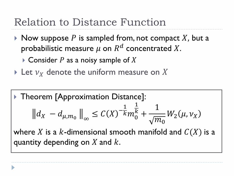
Relation to Distance Function

Now suppose 𝑃 is sampled from, not compact 𝑋, but a

probabilistic measure 𝜇 on 𝑅𝑑 concentrated 𝑋.

Consider 𝑃 as a noisy sample of 𝑋

Let 𝜈𝑋 denote the uniform measure on 𝑋

Theorem [Approximation Distance]:

𝑑𝑋 − 𝑑𝜇,𝑚0 ∞≤ 𝐶 𝑋 −

1𝑘𝑚0

1𝑘 +

1

𝑚0𝑊2 𝜇, 𝜈𝑋

where 𝑋 is a 𝑘-dimensional smooth manifold and 𝐶(𝑋) is a

quantity depending on 𝑋 and 𝑘.

Computational Aspect

Distance to measures can be approximated efficiently for

a set of points P

[Guibas, Mérigot and Morozov, DCG 2013]

Can be extended to metric spaces, and build weighted

Cech / Rips complexes for reconstruction and homology

inference

[Buchet, Chazal, Oudot, Sheehy, 2013]

Outline




Sampling conditions


Topology inference

Homology inference

Handling noise



Two Additional Examples

Previously:

Homology inference: topological information of a space

Approximating cycles of shortest basis of the first

homology group

As an example of combining geometry and topology


As an example of approximating the topology of a scalar field

See separate slides for these two additional topics.

Summary

One example of the pipeline of approximating certain

topological structure from discrete samples

The components in the pipeline are quite generic

Many other issues too:

Stability

Efficiency

Sparsification

etc

Summary – cont.

Starting to have more interaction with statistics and

probability theory

E.g, [Balakrishnan et al., AISTATS 2012], [Bendich et al., SoDA 2012]

How to develop algorithms that integrating

computational geometry / topology ideas with statistics,

especially in data analysis?

References

Weak witnesses for Delaunay triangulations of submanifolds. D. Attali, H.

Edelsbrunner, and Y. Mileyko. Proc. ACM Sympos. on Solid and Physical

Modeling, 143–150 (2007)

Manifold reconstruction in arbitrary dimensions using witness complexes. D.

Boissonnat and L. J. Guibas and S. Y. Oudot. SoCG 194–203, (2007)

Efficient and Robust Topological Data Analysis on Metric Spaces. M. Buchet, F.

Chazal, S. Y. Oudot, D. Sheehy:. CoRR abs/1306.0039 (2013)

Geometric Inference. F. Chazal and D. Cohen-Steiner. Tesselations in the

Sciences, Springer-Verlag, (2013, to appear).

A sampling theory for compacts in Euclidean space . F. Chazal, D. Cohen-Steiner,

and A. Lieutier. Discrete Comput. Geom. 41, 461--479 (2009).

Geometric Inference for Probability Measures. F. Chazal, D. Cohen-Steiner, Q.

Mérigot. Foundations of Computational Mathematics 11(6): 733-751 (2011)

Stability and Computation of Topological Invariants of Solids in 𝑅𝑛. F. Chazal, A.

Lieutier. Discrete & Computational Geometry 37(4): 601-617 (2007)

References – cont.

Towards persistence-based reconstruction in Euclidean spaces. F. Chazal and S.

Oudot. Proc. Annu. Sympos. Comput. Geom. (2008), 232--241.

Proximity of persistence modules and their diagrams. F. Chazal, D. Cohen-

Steiner, M. Glisse, L. Guibas, and S. Oudot. Proc. 25th Annu. Sympos.

Comput. Geom. (2009), 237-246.

A weak definition of Delaunay triangulation. Vin de Silva. CoRR

cs.CG/0310031 (2003)

Topological estimation using witness complexes. V. de Silva, G. Carlsson,

Symposium on Point-Based Graphics,, 2004

Topological estimation using witness complexes. Vin de Silva and Gunnar

Carlsson. Eurographics Sympos. Point-Based Graphics (2004).

Curve and Surface Reconstruction : Algorithms with Mathematical Analysis. Tamal.

K. Dey. Cambridge University Press, 2006.

Graph induced complex on point data. T. K. Dey, F. Fan, and Y. Wang. to appear

in 29th Annual Sympos. Comput. Geom. (SoCG) 2013.


Witnessed k-Distance. L. J. Guibas, D. Morozov, Q. Mérigot. Discrete &

Computational Geometry 49(1): 22-45 (2013)

Reconstructing using witness complexes, L. J. Guibas and S. Y. Oudot. Discrete

Comput. Geom. 30, 325–356 (2008).

Any open bounded subset of 𝑅𝑛 has the same homotopy type as its medial axis.

A. Lieutier. Computer-Aided Design 36(11): 1029-1046 (2004)

Finding the homology of submanifolds with high confidence from random samples.

P. Niyogi, S. Smale, and S. Weinberger. Discrete Comput. Geom., 39, 419--

441 (2008).

Geodesic delaunay triangulations in bounded planar domains. S. Oudot, L. J.

Guibas, J. Gao and Y. Wang. ACM Trans. Alg. 6 (4): 2010.


Minimax rates for homology inference. S. Balakrishnan, A. Rinaldo, D. Sheehy, A.

Singh, L. A. Wasserman. AISTATS 2012: 64-72

Local Homology Transfer and Stratification Learning. P. Bendich, B. Wang and S.

Mukherjee. ACM-SIAM Symposium on Discrete Algorithms, (2012).

Greedy optimal homotopy and homology generators. J. Erickson and K.

Whittlesey. Proc. Sixteenth ACM-SIAM Sympos. Discrete Algorithms (2005),

1038--1046.

Approximating cycles in a shortest basis of the first homology group from point

data. T. K. Dey, J. Sun, and Y. Wang. Inverse Problems, 27 (2011).

Reeb graphs: Approximation and Persistence. T. K. Dey and Y. Wang., Discrete

Comput. Geom (DCG) 2013.

some topics in computational topology - duke universitysayan/jmm/computational.pdf · some topics...

Documents