sonar sensor interpretation and infrared image fusion for mobile

4

Sonar Sensor Interpretation and Infrared Image Fusion for Mobile Robotics

Mark Hinders, Wen Gao and William Fehlman Department of Applied Science, The College of William & Mary in Virginia

NDE Lab @ 106 Jamestown Road, Williamsburg, VA 23187-8795

1. Introduction

The goal of our research is to give mobile robots the ability to deal with real world instructions outdoors such as “Go down to the big tree and turn left.” Inherent in such a paradigm is the robot being able to recognize a “big tree” and do it in unstructured environments without too many pre-mapped fixed landmarks. Ultimately we envision mobile robots that unobtrusively mix in with pedestrian traffic and hence traveling primarily at a walking pace. With regard to sensors this is a different problem from robots designed to drive on roadways, since the necessary range of sensors is tied to the speed of the robot. It’s also important to note that small mobile robots that are intended to mix with pedestrian traffic must normally travel at the same speed as the pedestrians, even if they occasionally scurry quickly down a deserted alley or slow way down to traverse a tricky obstacle, because people resent having to go around a slow robot while they are also easily startled by machines such as Segways that overtake them without warning. At walking speeds the range of sonar at about 50kHz is optimal, and there are none of the safety concerns one might have with lidar, for example. This type of sonar is precisely what bats use for echolocation; the goal of our research is to employ sonar sensors to allow mobile robots to recognize objects in the everyday environment based on simple signal processing algorithms tied to the physics of how the sonar backscatters from various objects. Our primary interest is for those sensors that can function well outdoors without regard to lighting conditions or even in the absence of daylight. We have built several 3D sonar scanning systems packaged as sensor heads on mobile robots, so that we are able to traverse the local environment and easily acquire 3D sonar scans of typical objects and structures. Of course sonar of the type we’re exploring is not new. As early as 1773 it was observed that bats could fly freely in a dark room and pointed out that hearing was an important component of bats’ orientation and obstacle avoidance capabilities (Au, 1993). By 1912 it was suggested that bats use sounds inaudible to humans to detect objects (Maxim, 1912) but it wasn’t until 1938 that Griffin proved that bats use ultrasound to detect objects (Griffin, 1958). More recently, Roman Kuc and his co-workers (Barshan & Kuc, 1992; Kleeman & Kuc, 1995) developed a series of active wide-beam sonar systems that mimic the sensor configuration of echolocating bats, which can distinguish planes, corners and edges necessary to navigate indoors. Catherine Wykes and her colleagues (Chou & Wykes, 1999) have built a prototype integrated ultrasonic/vision sensor that uses an off-the-shelf CCD camera and a four-element sonar phased array sensor that enables the camera to be calibrated using data from

Source: Mobile Robots: Perception & Navigation, Book edited by: Sascha Kolski, ISBN 3-86611-283-1, pp. 704, February 2007, Plv/ARS, Germany

Ope

n A

cces

s D

atab

ase

ww

w.i-

tech

onlin

e.co

m

70 Mobile Robots, Perception & Navigation

the ultrasonic sensor. Leslie Kay (Kay, 2000) has developed and commercialized high-resolution octave band air sonar for spatial sensing and object imaging by blind persons. Phillip McKerrow and his co-workers (McKerrow & Harper, 1999; Harper & McKerrow, 2001; Ratner & McKerrow, 2003) have been focused on outdoor navigation and recognition of leafy plants with sonar. Other research groups are actively developing algorithms for the automatic interpretation of sensor data (Leonard & Durrant-Whyte, 1992; Crowley, 1985; Dror et al., 1995; Jeon & Kim, 2001). Our goal is to bring to bear a high level knowledge of the physics of sonar backscattering and then to apply sophisticated discrimination methods of the type long established in other fields (Rosenfeld & Kak, 1982; Theodoridis & Koutroumbas, 1998; Tou, 1968). In section 2 we describe an algorithm to distinguish big trees, little trees and round metal poles based on the degree of asymmetry in the backscatter as the sonar beam is swept across them. The asymmetry arises from lobulations in the tree cross section and/or roughness of the bark. In section 3 we consider extended objects such as walls, fences and hedges of various types which may be difficult to differentiate under low light conditions. We key on features such as side peaks due to retroreflectors formed by the pickets and posts which can be counted via a deformable template signal processing scheme. In section 4 we discuss the addition of thermal infrared imagery to the sonar information and the use of Bayesian methods that allow us to make use of a priori knowledge of the thermal conduction and radiation properties of common objects under a variety of weather conditions. In section 5 we offer some conclusions and discuss future research directions.

2. Distinguishing Trees & Poles Via Ultrasound Backscatter Asymmetry

In this section we describe an algorithm to automatically distinguish trees from round metal poles with a sonar system packaged on a mobile robot. A polynomial interpolation of the square root of the backscattered signal energy vs. scan angle is first plotted. Asymmetry and fitting error are then extracted for each sweep across the object, giving a single point in an abstract phase space. Round metal poles are nearer to the origin than are trees, which scatter the sonar more irregularly due to lobulations and/or surface roughness. Results are shown for 20 trees and 10 metal poles scanned on our campus.

Fig. 1. Diagram of the scanner head. The dotted lines represent the two axes that the camera and ultrasound transducer rotate about.

Ultrasound

Transducer

IR Camera Stepper

Motors

Sonar Sensor Interpretation and Infrared Image Fusion for Mobile Robotics 71

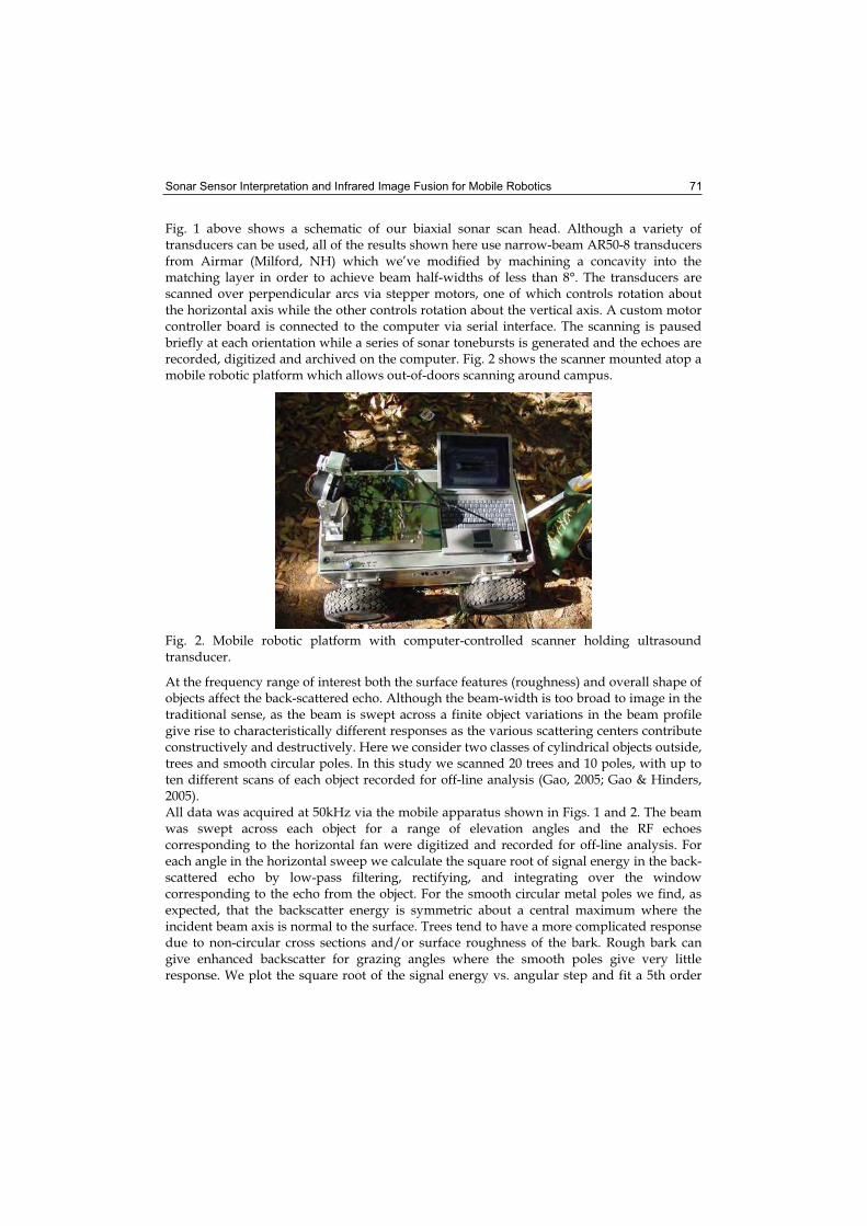
Fig. 1 above shows a schematic of our biaxial sonar scan head. Although a variety of transducers can be used, all of the results shown here use narrow-beam AR50-8 transducers from Airmar (Milford, NH) which we’ve modified by machining a concavity into the matching layer in order to achieve beam half-widths of less than 8°. The transducers are scanned over perpendicular arcs via stepper motors, one of which controls rotation about the horizontal axis while the other controls rotation about the vertical axis. A custom motor controller board is connected to the computer via serial interface. The scanning is paused briefly at each orientation while a series of sonar tonebursts is generated and the echoes are recorded, digitized and archived on the computer. Fig. 2 shows the scanner mounted atop a mobile robotic platform which allows out-of-doors scanning around campus.

Fig. 2. Mobile robotic platform with computer-controlled scanner holding ultrasound transducer.

At the frequency range of interest both the surface features (roughness) and overall shape of objects affect the back-scattered echo. Although the beam-width is too broad to image in the traditional sense, as the beam is swept across a finite object variations in the beam profile give rise to characteristically different responses as the various scattering centers contribute constructively and destructively. Here we consider two classes of cylindrical objects outside, trees and smooth circular poles. In this study we scanned 20 trees and 10 poles, with up to ten different scans of each object recorded for off-line analysis (Gao, 2005; Gao & Hinders, 2005).All data was acquired at 50kHz via the mobile apparatus shown in Figs. 1 and 2. The beam was swept across each object for a range of elevation angles and the RF echoes corresponding to the horizontal fan were digitized and recorded for off-line analysis. For each angle in the horizontal sweep we calculate the square root of signal energy in the back-scattered echo by low-pass filtering, rectifying, and integrating over the window corresponding to the echo from the object. For the smooth circular metal poles we find, as expected, that the backscatter energy is symmetric about a central maximum where the incident beam axis is normal to the surface. Trees tend to have a more complicated response due to non-circular cross sections and/or surface roughness of the bark. Rough bark can give enhanced backscatter for grazing angles where the smooth poles give very little response. We plot the square root of the signal energy vs. angular step and fit a 5th order


polynomial to it. Smooth circular poles always give a symmetric (bell-shaped) central response whereas rough and/or irregular objects often give responses less symmetric about the central peak. In general, one sweep over an object is not enough to tell a tree from a pole. We need a series of scans for each object to be able to robustly classify them. This is equivalent to a robot scanning an object repeatedly as it approaches. Assuming that the robot has already adjusted its path to avoid the obstruction, each subsequent scan gives a somewhat different orientation to the target. Multiple looks at the target thus increase the robustness of our scheme for distinguishing trees from poles because trees have more variations vs. look angle than do round metal poles.

Fig. 3. Square root of signal energy plots of pole P1 when the sensor is (S1) 75cm (S2) 100cm (S3) 125cm (S4) 150cm (S5) 175cm (S6) 200cm (S7) 225cm (S8) 250cm (S9) 275cm from the pole.

Fig. 3 shows the square root of signal energy plots of pole P1 (a 14 cm diameter circular metal lamppost) from different distances and their 5th order polynomial interpolations. Each data point was obtained by low-pass filtering, rectifying, and integrating over the window corresponding to the echo from the object to calculate the square root of the signal energy as a measure of backscatter strength. For each object 16 data points were calculated as the beam was swept across it. The polynomial fits to these data are shown by the solid curve for 9 different scans. All of the fits in Fig. 3 are symmetric (bell-shaped) near the central scan angle, which is characteristic of a smooth circular pole. Fig. 4 shows the square root of signal energy plots of tree T14, a 19 cm diameter tree which has a relatively smooth surface. Nine scans are shown from different distances along with their 5th order


polynomial interpolations. Some of these are symmetric (bell-shaped) and some are not, which is characteristic of a round smooth-barked tree.

Fig. 4. Square root of signal energy plots of tree T14 when the sensor is (S1) 75cm (S2) 100cm (S3) 125cm (S4) 150cm (S5) 175cm (S6) 200cm (S7) 225cm (S8) 250cm (S9) 275cm from the tree.

Fig. 5 on the following page shows the square root of signal energy plots of tree T18, which is a 30 cm diameter tree with a rough bark surface. Nine scans are shown, from different distances, along with their 5th order polynomial interpolations. Only a few of the rough-bark scans are symmetric (bell-shaped) while most are not, which is characteristic of a rough and/or non-circular tree. We also did the same procedure for trees T15-T17, T19, T20 and poles P2, P3, P9, P10. We find that if all the plots are symmetric bell-shaped it can be confidently identified as a smooth circular pole. If some are symmetric bell-shaped while some are not, it can be identified as a tree. Of course our goal is to have the computer distinguish trees from poles automatically based on the shapes of square root of signal energy plots. The feature vector x we choose contains two elements: Asymmetry and Deviation. If we let x1 represent Asymmetry and x2 represent Deviation, the feature vector can be written as x=[x1, x2]. For example, Fig. 6 on the following page is the square root of signal energy plot of pole P1 when the distance is 200cm. For x1 we use Full-Width Half Maximum (FWHM) to define asymmetry. We cut the full width half-maximum into two to get the left width L1 and right width L2. Asymmetry is defined as the difference between L1 and L2 divided by FWHM, which is |L1-L2|/|L1+L2|. The Deviation x2 we define as the average distance from the experimental


data point to the fitted data point at the same x-axis location, divided by the total height of the fitted curve H. In this case, there are 16 experimental data points, so Deviation =

(|d1|+|d2|+...+|d16|)/(16H). For the plot above, we get Asymmetry=0.0333, which means the degree of asymmetry is small. We also get Deviation=0.0467, which means the degree of deviation is also small.

Fig. 5. Square root of signal energy plots of tree T18 when the sensor is (S1) 75cm (S2) 100cm (S3) 125cm (S4) 150cm (S5) 175cm (S6) 200cm (S7) 225cm (S8) 250cm (S9) 275cm from the tree.

Fig. 6. Square root of signal energy plot of pole P1at a distance of 200cm.


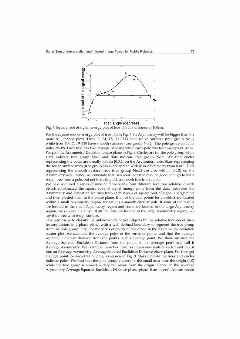
Fig. 7. Square root of signal energy plot of tree T14 at a distance of 100cm.

For the square root of energy plot of tree T14 in Fig. 7, its Asymmetry will be bigger than the more bell-shaped plots. Trees T1-T4, T8, T11-T13 have rough surfaces (tree group No.1) while trees T5-T7, T9-T10 have smooth surfaces (tree group No.2). The pole group contains poles P4-P8. Each tree has two sweeps of scans while each pole has four sweeps of scans. We plot the Asymmetry-Deviation phase plane in Fig. 8. Circles are for the pole group while stars indicate tree group No.1 and dots indicate tree group No.2. We find circles representing the poles are usually within [0,0.2] on the Asymmetry axis. Stars representing the rough surface trees (tree group No.1) are spread widely in Asymmetry from 0 to 1. Dots representing the smooth surface trees (tree group No.2) are also within [0,0.2] on the Asymmetry axis. Hence, we conclude that two scans per tree may be good enough to tell a rough tree from a pole, but not to distinguish a smooth tree from a pole. We next acquired a series of nine or more scans from different locations relative to each object, constructed the square root of signal energy plots from the data, extracted the Asymmetry and Deviation features from each sweep of square root of signal energy plots and then plotted them in the phase plane. If all of the data points for an object are located within a small Asymmetry region, we say it’s a smooth circular pole. If some of the results are located in the small Asymmetry region and some are located in the large Asymmetry region, we can say it’s a tree. If all the dots are located in the large Asymmetry region, we say it’s a tree with rough surface. Our purpose is to classify the unknown cylindrical objects by the relative location of their feature vectors in a phase plane, with a well-defined boundary to segment the tree group from the pole group. First, for the series of points of one object in the Asymmetry-Deviation scatter plot, we calculate the average point of the series of points and find the average squared Euclidean distance from the points to this average point. We then calculate the Average Squared Euclidean Distance from the points to the average point and call it Average Asymmetry. We combine these two features into a new feature vector and plot it into an Average Asymmetry-Average Squared Euclidean Distance phase plane. We then get a single point for each tree or pole, as shown in Fig. 9. Stars indicate the trees and circles indicate poles. We find that the pole group clusters in the small area near the origin (0,0) while the tree group is spread widely but away from the origin. Hence, in the Average Asymmetry-Average Squared Euclidean Distance phase plane, if an object’s feature vector


is located in the small area near the origin, which is within [0,0.1] in Average Asymmetry and within [0,0.02] in Average Squared Euclidean Distance, we can say it’s a pole. If it is located in the area away from the origin, which is beyond the set area, we can say it’s a tree.

Fig. 8. Asymmetry-Deviation phase plane of the pole group and two tree groups. Circles indidate poles, dots indicate smaller smooth bark trees, and stars indicate the larger rough bark trees.

Fig. 9. Average Asymmetry-Average Squared Euclidean Distance phase plane of trees T14-T20 and poles P1-P3, P9 and P10.

3. Distinguishing Walls, Fences & Hedges with Deformable Templates

In this section we present an algorithm to distinguish several kinds of brick walls, picket fences and hedges based on the analysis of backscattered sonar echoes. The echo data are acquired by our mobile robot with a 50kHz sonar computer-controlled scanning system packaged as its sensor head (Figs. 1 and 2). For several locations along a wall, fence or hedge, fans of backscatter sonar echoes are acquired and digitized as the sonar transducer is swept over horizontal arcs. Backscatter is then plotted vs. scan angle, with a series of N-peak deformable templates fit to this data for each scan. The number of peaks in the best-fitting N-peak template indicates the presence and location of retro-reflectors, and allows automatic categorization of the various fences, hedges and brick walls.


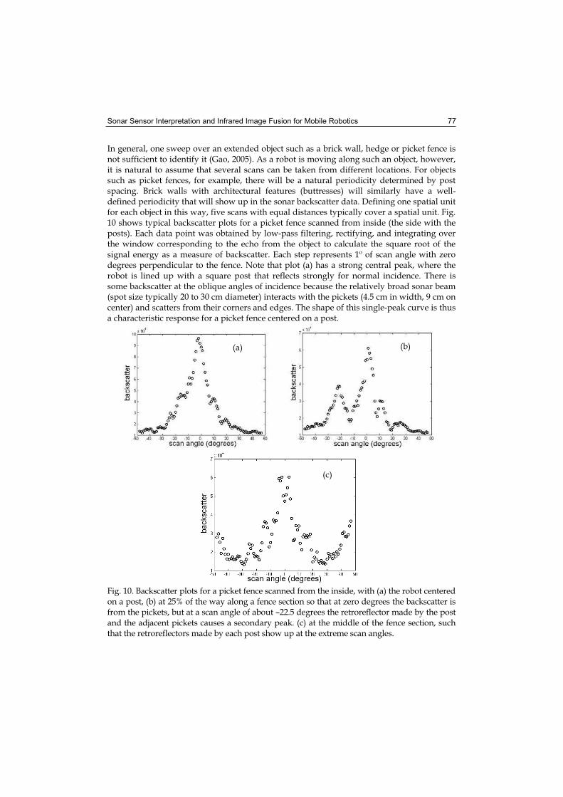
In general, one sweep over an extended object such as a brick wall, hedge or picket fence is not sufficient to identify it (Gao, 2005). As a robot is moving along such an object, however, it is natural to assume that several scans can be taken from different locations. For objects such as picket fences, for example, there will be a natural periodicity determined by post spacing. Brick walls with architectural features (buttresses) will similarly have a well-defined periodicity that will show up in the sonar backscatter data. Defining one spatial unit for each object in this way, five scans with equal distances typically cover a spatial unit. Fig. 10 shows typical backscatter plots for a picket fence scanned from inside (the side with the posts). Each data point was obtained by low-pass filtering, rectifying, and integrating over the window corresponding to the echo from the object to calculate the square root of the signal energy as a measure of backscatter. Each step represents 1º of scan angle with zero degrees perpendicular to the fence. Note that plot (a) has a strong central peak, where the robot is lined up with a square post that reflects strongly for normal incidence. There is some backscatter at the oblique angles of incidence because the relatively broad sonar beam (spot size typically 20 to 30 cm diameter) interacts with the pickets (4.5 cm in width, 9 cm on center) and scatters from their corners and edges. The shape of this single-peak curve is thus a characteristic response for a picket fence centered on a post.

Fig. 10. Backscatter plots for a picket fence scanned from the inside, with (a) the robot centered on a post, (b) at 25% of the way along a fence section so that at zero degrees the backscatter is from the pickets, but at a scan angle of about –22.5 degrees the retroreflector made by the post and the adjacent pickets causes a secondary peak. (c) at the middle of the fence section, such that the retroreflectors made by each post show up at the extreme scan angles.

(a) (b)

(c)


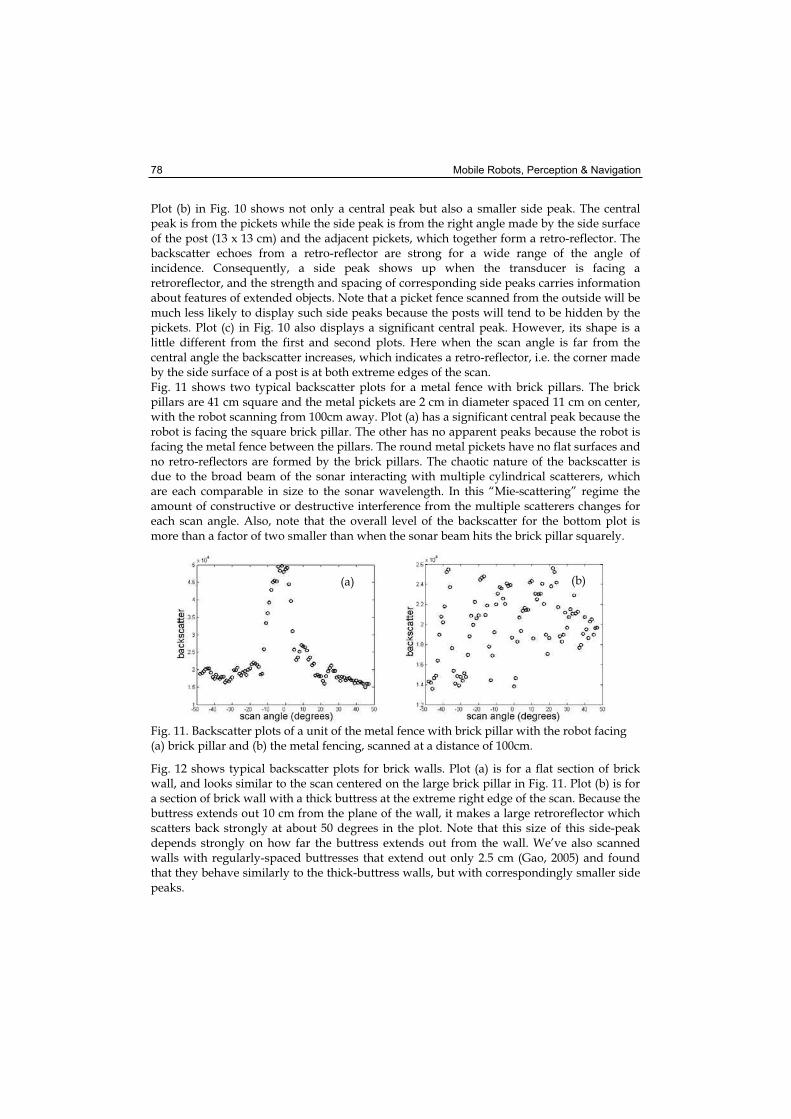
Plot (b) in Fig. 10 shows not only a central peak but also a smaller side peak. The central peak is from the pickets while the side peak is from the right angle made by the side surface of the post (13 x 13 cm) and the adjacent pickets, which together form a retro-reflector. The backscatter echoes from a retro-reflector are strong for a wide range of the angle of incidence. Consequently, a side peak shows up when the transducer is facing a retroreflector, and the strength and spacing of corresponding side peaks carries information about features of extended objects. Note that a picket fence scanned from the outside will be much less likely to display such side peaks because the posts will tend to be hidden by the pickets. Plot (c) in Fig. 10 also displays a significant central peak. However, its shape is a little different from the first and second plots. Here when the scan angle is far from the central angle the backscatter increases, which indicates a retro-reflector, i.e. the corner made by the side surface of a post is at both extreme edges of the scan. Fig. 11 shows two typical backscatter plots for a metal fence with brick pillars. The brick pillars are 41 cm square and the metal pickets are 2 cm in diameter spaced 11 cm on center, with the robot scanning from 100cm away. Plot (a) has a significant central peak because the robot is facing the square brick pillar. The other has no apparent peaks because the robot is facing the metal fence between the pillars. The round metal pickets have no flat surfaces and no retro-reflectors are formed by the brick pillars. The chaotic nature of the backscatter is due to the broad beam of the sonar interacting with multiple cylindrical scatterers, which are each comparable in size to the sonar wavelength. In this “Mie-scattering” regime the amount of constructive or destructive interference from the multiple scatterers changes for each scan angle. Also, note that the overall level of the backscatter for the bottom plot is more than a factor of two smaller than when the sonar beam hits the brick pillar squarely.

Fig. 11. Backscatter plots of a unit of the metal fence with brick pillar with the robot facing (a) brick pillar and (b) the metal fencing, scanned at a distance of 100cm.

Fig. 12 shows typical backscatter plots for brick walls. Plot (a) is for a flat section of brick wall, and looks similar to the scan centered on the large brick pillar in Fig. 11. Plot (b) is for a section of brick wall with a thick buttress at the extreme right edge of the scan. Because the buttress extends out 10 cm from the plane of the wall, it makes a large retroreflector which scatters back strongly at about 50 degrees in the plot. Note that this size of this side-peak depends strongly on how far the buttress extends out from the wall. We’ve also scanned walls with regularly-spaced buttresses that extend out only 2.5 cm (Gao, 2005) and found that they behave similarly to the thick-buttress walls, but with correspondingly smaller side peaks.

(a) (b)


Fig. 12 Backscatter plots of a unit of brick wall with thick buttress with the robot at a distance of 100cm facing (a) flat section of wall and (b) section including retroreflecting buttress at extreme left scan angle.

Fig. 13 Backscatter plot of a unit of hedge.

Fig. 13 shows a typical backscatter plot for a trimmed hedge. Note that although the level of the backscatter is smaller than for the picket fence and brick wall, the peak is also much broader. As expected the foliage scatters the sonar beam back over a larger range of angles. Backscatter data of this type was recorded for a total of seven distinct objects: the wood picket fence described above from inside (side with posts), that wood picket fence from outside (no posts), the metal fence with brick pillars described above, a flat brick wall, a trimmed hedge, and brick walls with thin (2.5 cm) and thick (10 cm) buttresses, respectively (Gao, 2005; Gao & Hinders, 2006). For those objects with spatial periodicity formed by posts or buttresses, 5 scans were taken over such a unit. The left- and right-most scans were centered on the post or buttress, and then three scans were taken evenly spaced in between. For typical objects scanned from 100 cm away with +/- 50 degrees scan angle the middle scans just see the retroreflectors at the extreme scan angles, while the scans 25% and 75% along the unit length only have a single side peak from the nearest retro-reflector. For those objects without such spatial periodicity a similar unit length was chosen for each with five evenly spaced scans taken as above. Analyzing the backscatter plots constructed from this data, we concluded that the different objects each have a distinct sequence of backscatter plots, and that it should be possible to automatically distinguish such objects based on characteristic features in these backscatter plots. We have implemented a deformable

(a)(b)


template matching scheme to use this backscattering behaviour to differentiate the seven types of objects. A deformable template is a simple mathematically defined shape that can be fit to the data of interest without losing its general characteristics (Gao, 2005). For example, for a one-peak deformable template, its peak location may change when fitting to different data, but it always preserves its one peak shape characteristic. For each backscatter plot we next create a series of deformable N-peak templates (N=1, 2, 3… Nmax) and then quantify how well the templates fit for each N. Obviously a 2-peak template (N=2) will fit best to a backscatter plot with two well-defined peaks. After consideration of a large number of backscatter vs. angle plots of the types in the previous figures, we have defined a general sequence of deformable templates in the following manner. For one-peak templates we fit quintic functions to each of the two sides of the peak, located at xp, each passing through the peak as well as the first and last data points, respectively. Hence, the left part of the one-peak template is defined by the

function ( ) )(5

1 LL xBxxcy +−= which passes through the peak giving( )51

)()(

Lp

Lp

xx

xBxBc

−

−= .

Here B(x) is the value of the backscatter at angle x. Therefore, the one-peak template function defined over the range from x = xL to x = xp is

( )( ) )(

)()(5

5 LL

Lp

LpxBxx

xx

xBxBy +−

−

−= . (1a)

The right part of the one peak template is defined similarly over the range between x = xp to

x = xR, i.e. the function ( ) ( )RR xBxxcy +−=5

2 , with c2 given as ( ) ( )

( )52

Rp

Rp

xx

xBxBc

−

−= .

Therefore, the one-peak template function of the right part is

( ) ( )

( )( ) ( )RR

Rp

RpxBxx

xx

xBxBy +−

−

−=

5

5. (1b)

For the double-peak template, the two selected peaks xp1 and xp2 as well as the location of the valley xv between the two backscatter peaks separate the double-peak template into four regions with xp1<xv<xp2. The double peak template is thus comprised of four parts, defined as second-order functions between the peaks and quintic functions outbound of the two peaks.

( )( ) )(

)()(5

51

1LL

Lp

LpxBxx

xx

xBxBy +−

−

−= Lx x xp1

( )( ) )(

)()(2

21

1vv

vp

vpxBxx

xx

xBxBy +−

−

−= xp1 x xv

( )( ) )(

)()(2

22

2vv

vp

vpxBxx

xx

xBxBy +−

−

−= xv x xp2

( )( ) )(

)()(5

52

2RR

Rp

RpxBxx

xx

xBxBy +−

−

−= xp2 x xR


In the two middle regions, shapes of quadratic functions are more similar to the backscatter plots. Therefore, quadratic functions are chosen to form the template instead of quintic functions. Fig. 14 shows a typical backscatter plot for a picket fence as well as the corresponding single- and double-peak templates. The three, four, five, …, -peak template building follows the same procedure, with quadratic functions between the peaks and quintic functions outboard of the first and last peaks.

Fig. 14. Backscatter plots of the second scan of a picket fence and its (a) one-peak template (b) two-peak template

In order to characterize quantitatively how well the N-peak templates each fit a given backscatter plot, we calculate the sum of the distances from the backscatter data to the template at the same scan angle normalized by the total height H of the backscatter plot and the number of scan angles. For each backscatter plot, this quantitative measure of goodness of fit (Deviation) to the template is calculated automatically for N=1 to N=9 depending upon how many distinct peaks are identified by our successive enveloping and peak-picking algorithm (Gao, 2005). We can then calculate Deviation vs. N and fit a 4th order polynomial to each. Where the deviation is smallest indicates the N-peak template which fits best. We do this on the polynomial fit rather than on the discrete data points in order to automate the process, i.e. we differentiate the Deviation vs. N curve and look for zero crossings by setting a threshold as the derivative approaches zero from the negative side. This corresponds to the deviation decreasing with increasing N and approaching the minimum deviation, i.e. the best-fit N-peak template. Because the fit is a continuous curve we can consider non-integer N, i.e. the derivative value of the 4th order polynomial fitting when the template value is N+0.5. This describes how the 4th order polynomial fitting changes from N-peak template fitting to (N+1)-peak template fitting. If it is positive or a small negative value, it means that in going from the N-peak template to the (N+1)-peak template, the fitting does not improve much and the N-peak template is taken to be better than the (N+1)-peak template. Accordingly, we first set a threshold value and calculate these slopes at both integer and half-integer values of N. The threshold value is set to be -0.01 based on experience with data sets of this type, although this threshold could be considered as an adjustable parameter. We then check the value of the slopes in order. The N-peak-template is chosen to be the best-fit template when the slope at (N+0.5) is bigger than the threshold value of -0.01 for the first time. We also set some auxiliary rules to better to pick the right number of peaks. The first rule helps the algorithm to key on retroreflectors and ignore unimportant scattering centers: if

(a) (b)


the height ratio of a particular peak to the highest peak is less than 0.2, it is not counted as a peak. Most peaks with a height ratio less than 0.2 are caused by small scattering centers related to the rough surface of the objects, not by a retro-reflector of interest. The second rule is related to the large size of the sonar beam: if the horizontal difference of two peaks is less than 15 degrees, we merge them into one peak. Most of the double peaks with angular separation less than 15 degrees are actually caused by the same major reflector interacting with the relatively broad sonar beam. Two 5-dimensional feature vectors for each object are next formed. The first is formed from the numbers of the best fitting templates, i.e. the best N for each of the five scans of each object. The second is formed from the corresponding Deviation for each of those five scans. For example, for a picket fence scanned from inside, the two 5-dimensional feature vectors are N=[1,2,3,2,1] and D=[0.0520, 0.0543, 0.0782, 0.0686, 0.0631]. For a flat brick wall, they are N=[1,1,1,1,1] and D=[0.0549, 0.0704, 0.0752, 0.0998, 0.0673].The next step is to determine whether an unknown object can be classified based on these two 5-dimensional feature vectors. Feature vectors with higher dimensions (>3) are difficult to display visually, but we can easily deal with them in a hyper plane. The Euclidean distance of a feature vector in the hyper plane from an unknown object to the feature vector of a known object is thus calculated and used to determine if the unknown object is similar to any of the objects we already know. For both 5-dimensional feature vectors of an unknown object, we first calculate their Euclidean distances to the corresponding template feature vectors of a picket fence. N1 = |Nunknown - Npicketfence| is the Euclidean distance between the N vector of the unknown object Nunknown to the N vector of the picket fence Npicketfence. Similarly, D1 = | Nunknown - Npicketfence | is the Euclidean distance between the D vectors of the unknown object Nunknown

and the picket fence Npicketfence. We then calculate these distances to the corresponding feature vectors of a flat brick wall N2, D2, their distances to the two feature vectors of a hedge N3, D3 and so on. The unknown object is then classified as belonging to the kinds of objects whose two feature vectors are nearest to it, which means both N and D are small. Fig. 15 is an array of bar charts showing these Euclidean distances of two feature vectors of a unknown objects to the two feature vectors of seven objects we already know. The horizontal axis shows different objects numbered according to“1” for picket fence scanned from the inside “2” for a flat brick wall“3” for a trimmed hedge “4” for a brick wall with thin buttress “5” for a brick wall with thick buttress “6” for a metal fence with brick pillar and“7” for the picket fence scanned from the outside. The vertical axis shows the Euclidean distances of feature vectors of an unknown object to the 7 objects respectively. For each, the height of black bar and grey bar at object No.1 represent N1and 10 D1 respectively while the height of black bar and grey bar at object No.2 represent N2 and 10 D2 respectively, and so on. In the first chart both the black bar and grey bar are the shortest when comparing to the N, D vectors of a picket fence scanned from inside. Therefore, we conclude that this unknown object is a picket fence scanned from inside, which it is. Note that the D values have been scaled by a factor of ten to make the bar charts more readable. The second bar chart in Fig. 15 has both the black bar and grey bar the shortest when comparing to N, D vectors of object No.1 picket fence scanned from inside, which is what it is. The third bar chart in Fig. 15 has both the black bar and grey bar shortest when comparing to N, D vectors of object No.2 flat brick wall and object No.4 brick wall with thin buttress. That means the most probable kinds of the


unknown object are flat brick wall or brick wall with thin buttress. Actually it is a flat brick wall.

Fig. 15. N (black bar) and 10 D (gray bar) for fifteen objects compared to the seven known objects: 1 picket fence from inside, 2 flat brick wall, 3 hedge, 4 brick wall with thin buttress, 5 brick wall with thick buttress, 6 metal fence with brick pillar, 7 picket fence from outside.

Table 1 displays the results of automatically categorizing two additional scans of each of these seven objects. In the table, the + symbols indicate the correct choices and the x


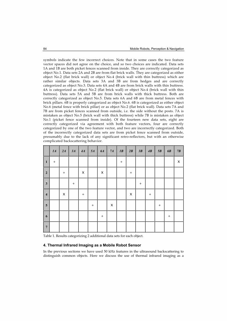
symbols indicate the few incorrect choices. Note that in some cases the two feature vector spaces did not agree on the choice, and so two choices are indicated. Data sets 1A and 1B are both picket fences scanned from inside. They are correctly categorized as object No.1. Data sets 2A and 2B are from flat brick walls. They are categorized as either object No.2 (flat brick wall) or object No.4 (brick wall with thin buttress) which are rather similar objects. Data sets 3A and 3B are from hedges and are correctly categorized as object No.3. Data sets 4A and 4B are from brick walls with thin buttress. 4A is categorized as object No.2 (flat brick wall) or object No.4 (brick wall with thin buttress). Data sets 5A and 5B are from brick walls with thick buttress. Both are correctly categorized as object No.5. Data sets 6A and 6B are from metal fences with brick pillars. 6B is properly categorized as object No.6. 6B is categorized as either object No.6 (metal fence with brick pillar) or as object No.2 (flat brick wall). Data sets 7A and 7B are from picket fences scanned from outside, i.e. the side without the posts. 7A is mistaken as object No.5 (brick wall with thick buttress) while 7B is mistaken as object No.1 (picket fence scanned from inside). Of the fourteen new data sets, eight are correctly categorized via agreement with both feature vectors, four are correctly categorized by one of the two feature vector, and two are incorrectly categorized. Both of the incorrectly categorized data sets are from picket fence scanned from outside, presumably due to the lack of any significant retro-reflectors, but with an otherwise complicated backscattering behavior.

1A 2A 3A 4A 5A 6A 7A 1B 2B 3B 4B 5B 6B 7B

1 + + X

2 + X X +

3 + +

4 X + X +

5 + X +

6 + +

7

Table 1. Results categorizing 2 additional data sets for each object.

4. Thermal Infrared Imaging as a Mobile Robot Sensor

In the previous sections we have used 50 kHz features in the ultrasound backscattering to distinguish common objects. Here we discuss the use of thermal infrared imaging as a


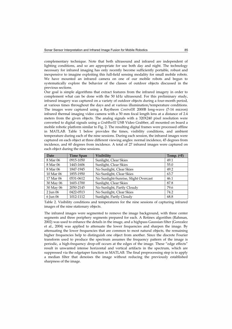
complementary technique. Note that both ultrasound and infrared are independent of lighting conditions, and so are appropriate for use both day and night. The technology necessary for infrared imaging has only recently become sufficiently portable, robust and inexpensive to imagine exploiting this full-field sensing modality for small mobile robots. We have mounted an infrared camera on one of our mobile robots and begun to systematically explore the behavior of the classes of outdoor objects discussed in the previous sections. Our goal is simple algorithms that extract features from the infrared imagery in order to complement what can be done with the 50 kHz ultrasound. For this preliminary study, infrared imagery was captured on a variety of outdoor objects during a four-month period, at various times throughout the days and at various illumination/temperature conditions. The images were captured using a Raytheon ControlIR 2000B long-wave (7-14 micron) infrared thermal imaging video camera with a 50 mm focal length lens at a distance of 2.4 meters from the given objects. The analog signals with a 320X240 pixel resolution were converted to digital signals using a GrabBeeIII USB Video Grabber, all mounted on board a mobile robotic platform similar to Fig. 2. The resulting digital frames were processed offline in MATLAB. Table 1 below provides the times, visibility conditions, and ambient temperature during each of the nine sessions. During each session, the infrared images were captured on each object at three different viewing angles: normal incidence, 45 degrees from incidence, and 60 degrees from incidence. A total of 27 infrared images were captured on each object during the nine sessions.

Date Time Span Visibility Temp. (oF)

8 Mar 06 0915-1050 Sunlight, Clear Skies 49.1

8 Mar 06 1443-1606 Sunlight, Clear Skies 55.0

8 Mar 06 1847-1945 No Sunlight, Clear Skies 49.2

10 Mar 06 1855-1950 No Sunlight, Clear Skies 63.7

17 Mar 06 0531-0612 No Sunlight-Sunrise, Slight Overcast 46.1

30 May 06 1603-1700 Sunlight, Clear Skies 87.8

30 May 06 2050-2145 No Sunlight, Partly Cloudy 79.6

2 Jun 06 0422-0513 No Sunlight, Clear Skies 74.2

6 Jun 06 1012-1112 Sunlight, Partly Cloudy 68.8

Table 2. Visibility conditions and temperatures for the nine sessions of capturing infrared images of the nine stationary objects.

The infrared images were segmented to remove the image background, with three center segments and three periphery segments prepared for each. A Retinex algorithm (Rahman, 2002) was used to enhance the details in the image, and a highpass Gaussian filter (Gonzalez et al., 2004) was applied to attenuate the lower frequencies and sharpen the image. By attenuating the lower frequencies that are common to most natural objects, the remaining higher frequencies help to distinguish one object from another. Since the discrete Fourier transform used to produce the spectrum assumes the frequency pattern of the image is periodic, a high-frequency drop-off occurs at the edges of the image. These “edge effects” result in unwanted intense horizontal and vertical artifacts in the spectrum, which are suppressed via the edgetaper function in MATLAB. The final preprocessing step is to apply a median filter that denoises the image without reducing the previously established sharpness of the image.


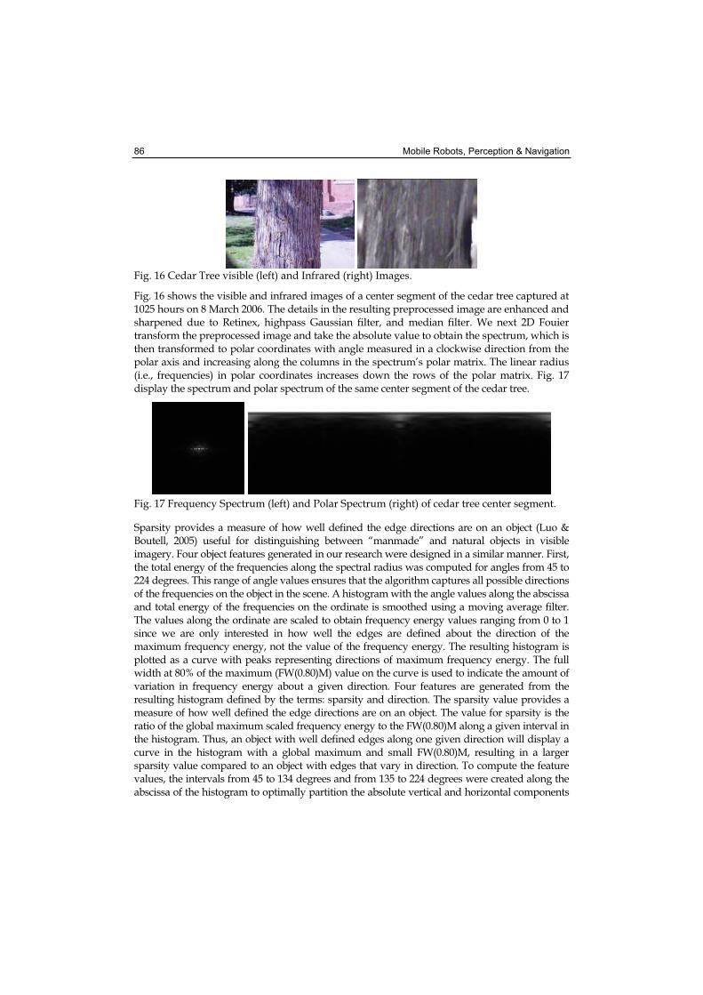
Fig. 16 Cedar Tree visible (left) and Infrared (right) Images.

Fig. 16 shows the visible and infrared images of a center segment of the cedar tree captured at 1025 hours on 8 March 2006. The details in the resulting preprocessed image are enhanced and sharpened due to Retinex, highpass Gaussian filter, and median filter. We next 2D Fouier transform the preprocessed image and take the absolute value to obtain the spectrum, which is then transformed to polar coordinates with angle measured in a clockwise direction from the polar axis and increasing along the columns in the spectrum’s polar matrix. The linear radius (i.e., frequencies) in polar coordinates increases down the rows of the polar matrix. Fig. 17 display the spectrum and polar spectrum of the same center segment of the cedar tree.

Fig. 17 Frequency Spectrum (left) and Polar Spectrum (right) of cedar tree center segment.

Sparsity provides a measure of how well defined the edge directions are on an object (Luo & Boutell, 2005) useful for distinguishing between “manmade” and natural objects in visible imagery. Four object features generated in our research were designed in a similar manner. First, the total energy of the frequencies along the spectral radius was computed for angles from 45 to 224 degrees. This range of angle values ensures that the algorithm captures all possible directions of the frequencies on the object in the scene. A histogram with the angle values along the abscissa and total energy of the frequencies on the ordinate is smoothed using a moving average filter. The values along the ordinate are scaled to obtain frequency energy values ranging from 0 to 1 since we are only interested in how well the edges are defined about the direction of the maximum frequency energy, not the value of the frequency energy. The resulting histogram is plotted as a curve with peaks representing directions of maximum frequency energy. The full width at 80% of the maximum (FW(0.80)M) value on the curve is used to indicate the amount of variation in frequency energy about a given direction. Four features are generated from the resulting histogram defined by the terms: sparsity and direction. The sparsity value provides a measure of how well defined the edge directions are on an object. The value for sparsity is the ratio of the global maximum scaled frequency energy to the FW(0.80)M along a given interval in the histogram. Thus, an object with well defined edges along one given direction will display a curve in the histogram with a global maximum and small FW(0.80)M, resulting in a larger sparsity value compared to an object with edges that vary in direction. To compute the feature values, the intervals from 45 to 134 degrees and from 135 to 224 degrees were created along the abscissa of the histogram to optimally partition the absolute vertical and horizontal components


in the spectrum. The sparsity value along with its direction are computed for each of the partitioned intervals. A value of zero is provided for both the sparsity and direction if there is no significant frequency energy present in the given interval to compute the FW(0.80)M. By comparing the directions (in radians) of the maximum scaled frequency energy along each interval, four features are generated: Sparsity about Maximum Frequency Energy (1.89 for tree vs. 2.80 for bricks), Direction of Maximum Frequency Energy (3.16 for tree vs. 1.57 for bricks), Sparsity about Minimum Frequency Energy (0.00 for tree vs. 1.16 for bricks), Direction of Minimum Frequency Energy (0.00 for tree vs. 3.14 for bricks). Fig. 19 below compares the scaled frequency energy histograms for the cedar tree and brick wall (Fig. 18), respectively.

Fig. 18. Brick Wall Infrared (left) and Visible (right) Images.

As we can see in the histogram plot of the cedar tree (Fig. 19, left) the edges are more well defined in the horizontal direction, as expected. Furthermore, the vertical direction presents no significant frequency energy. On the other hand, the results for the brick wall (Fig. 19, right) imply edge directions that are more well defined in the vertical direction. The brick wall results in a sparsity value and direction associated with minimum frequency energy. Consequently, these particular results would lead to features that could allow us to distinguish the cedar tree from the brick wall. Curvature provides a measure to distinguish cylindrical shaped objects from flat objects (Sakai & Finkel, 1995) since the ratio of the average peak frequency between the periphery and the center of an object in an image is strongly correlated with the degree of surface curvature. Increasing texture compression in an image yields higher frequency peaks in the spectrum. Consequently, for a cylindrically shaped object, we should see more texture compression and corresponding higher frequency peaks in the spectrum of the object’s periphery compared to the object’s center.

0.5 1 1.5 2 2.5 3 3.5 40.5

0.55

0.6

0.65

0.7

0.75

0.8

0.85

0.9

0.95

1Scaled Smoothed Frequency Energy (Cedar)

0.5 1 1.5 2 2.5 3 3.5 40.5

0.55

0.6

0.65

0.7

0.75

0.8

0.85

0.9

0.95

1Scaled Smoothed Frequency Energy (Brick Wall)

Fig. 19. Cedar (left) and Brick Wall (right) histogram plots.

To compute the curvature feature value for a given object, we first segment 80x80 pixel regions at the periphery and center of an object’s infrared image. The average peak frequency in the


horizontal direction is computed for both the periphery and center using the frequency spectrum. Since higher frequencies are the primary contributors in determining curvature, we only consider frequency peaks at frequency index values from 70 to 100. The curvature feature value is computed as the ratio of the average horizontal peak frequency in the periphery to that of the center. Fig. 20 compares the spectra along the horizontal of both the center and periphery segments for the infrared image of a cedar tree and a brick wall, respectively.

70 75 80 85 90 95 1001

2

3

4

5

6

7Cedar along Horizontal

Frequency

Am

plit

ude

Center

Periphery

70 75 80 85 90 95 100

0.8

1

1.2

1.4

1.6

1.8

2Brick Wall along Horizontal

Frequency

Am

plit

ude

Center

Periphery

Fig. 20 Cedar (left) and Brick Wall (right) Center vs. Periphery Frequency Energy Spectrum along Horizontal. The computed curvature value for the cedar tree is 2.14, while the computed curvature for the brick wall is 1.33.

As we can see in the left plot of Fig. 20 above, the periphery of the cedar tree’s infrared image has more energy at the higher frequencies compared to the center, suggesting that the object has curvature away from the observer. As we can see in the right plot of Fig. 20 above, there is not a significant difference between the energy in the periphery and center of the brick wall’s infrared image, suggesting that the object does not have curvature.

5. Summary and Future Work

We have developed a set of automatic algorithms that use sonar backscattering data to distinguish extended objects in the campus environment by taking a sequence of scans of each object, plotting the corresponding backscatter vs. scan angle, extracting abstract feature vectors and then categorizing them in various phase spaces. We have chosen to perform the analysis with multiple scans per object as a balance between data processing requirements and robustness of the results. Although our current robotic scanner is parked for each scan and then moves to the next scan location before scanning again, it is not difficult to envision a similar mobile robotic platform that scans continuously while moving. It could then take ten or even a hundred scans while approaching a tree or while moving along a unit of a fence, for example. Based on our experience with such scans, however, we would typically expect only the characteristic variations in backscattering behavior described above. Hence, we would envision scans taken continuously as the robot moves towards or along an object, and once the dominant features are identified, the necessary backscatter plots could be processed in the manner described in the previous sections, with the rest of the data safely purged from memory. Our reason for performing this level of detailed processing is a scenario where an autonomous robot is trying to identify particular landmark objects, presumably under low-


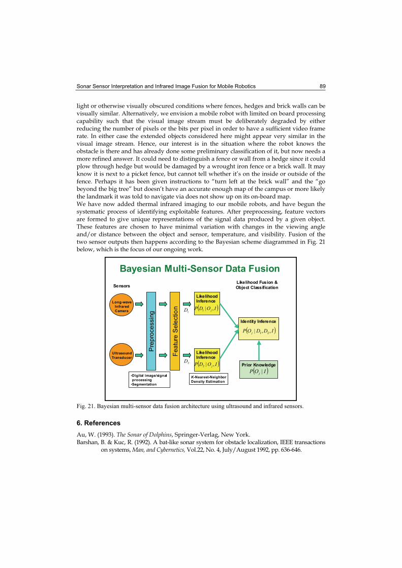
light or otherwise visually obscured conditions where fences, hedges and brick walls can be visually similar. Alternatively, we envision a mobile robot with limited on board processing capability such that the visual image stream must be deliberately degraded by either reducing the number of pixels or the bits per pixel in order to have a sufficient video frame rate. In either case the extended objects considered here might appear very similar in the visual image stream. Hence, our interest is in the situation where the robot knows the obstacle is there and has already done some preliminary classification of it, but now needs a more refined answer. It could need to distinguish a fence or wall from a hedge since it could plow through hedge but would be damaged by a wrought iron fence or a brick wall. It may know it is next to a picket fence, but cannot tell whether it’s on the inside or outside of the fence. Perhaps it has been given instructions to “turn left at the brick wall” and the “go beyond the big tree” but doesn’t have an accurate enough map of the campus or more likely the landmark it was told to navigate via does not show up on its on-board map. We have now added thermal infrared imaging to our mobile robots, and have begun the systematic process of identifying exploitable features. After preprocessing, feature vectors are formed to give unique representations of the signal data produced by a given object. These features are chosen to have minimal variation with changes in the viewing angle and/or distance between the object and sensor, temperature, and visibility. Fusion of the two sensor outputs then happens according to the Bayesian scheme diagrammed in Fig. 21 below, which is the focus of our ongoing work.

Ultrasound

Transducer

Long-wave

Infrared

Camera

SensorsLikelihood Fusion &

Object Classification

Fe

atu

re S

ele

ctio

n

LikelihoodInference

LikelihoodInference

2D

1D ( )IODP j ,|1

( )IODP j ,|2

Identity Inference

( )IDDOP j ,,| 21

Prior Knowledge

( )IOP j |

Pre

pro

ce

ssin

g

Bayesian Multi-Sensor Data Fusion

•Digital image/signal

processing

•Segmentation

K-Nearest-Neighbor

Density Estimation

Fig. 21. Bayesian multi-sensor data fusion architecture using ultrasound and infrared sensors.

6. References

Au, W. (1993). The Sonar of Dolphins, Springer-Verlag, New York. Barshan, B. & Kuc, R. (1992). A bat-like sonar system for obstacle localization, IEEE transactions

on systems, Man, and Cybernetics, Vol.22, No. 4, July/August 1992, pp. 636-646.


Chou, T. & Wykes, C. (1999). An integrated ultrasonic system for detection, recognition and measurement, Measurement, Vol. 26, No. 3, October 1999, pp. 179-190.

Crowley, J. (1985). Navigation for an intelligent mobile robot, IEEE Journal of Robotics and Automation, vol. RA-1, No. 1, March 1985, pp. 31-41.

Dror, I.; Zagaeski, M. & Moss, C. (1995). Three-dimensional target recognition via sonar: a neural network model, Neural Networks, Vol. 8, No. 1, pp. 149-160, 1995.

Gao, W. (2005). Sonar Sensor Interpretation for Ectogenous Robots, College of William and Mary, Department of Applied Science Doctoral Dissertation, April 2005.

Gao, W. & Hinders, M.K. (2005). Mobile Robot Sonar Interpretation Algorithm for Distinguishing Trees from Poles, Robotics and Autonomous Systems, Vol. 53, pp. 89-98.

Gao, W. & Hinders, M.K. (2006). Mobile Robot Sonar Deformable Template Algorithm for Distinguishing Fences, Hedges and Low Walls, Int. Journal of Robotics Research, Vol. 25, No. 2, pp. 135-146.

Gonzalez, R.C. (2004) Gonzalez, R. E. Woods & S. L. Eddins, Digital Image Processing using MALAB, Pearson Education, Inc.

Griffin, D. Listening in the Dark, Yale University Press, New Haven, CT. Harper, N. & McKerrow, P. (2001). Recognizing plants with ultrasonic sensing for mobile

robot navigation, Robotics and Autonomous Systems, Vol.34, 2001, pp.71-82. Jeon, H. & Kim, B. (2001). Feature-based probabilistic map building using time and amplitude

information of sonar in indoor environments, Robotica, Vol. 19, 2001, pp. 423-437. Kay, L. (2000). Auditory perception of objects by blind persons, using a bioacoustic high

resolution air sonar, Journal of the Acoustical Society of America Vol. 107, No. 6, June 2000, pp. 3266-3275.

Kleeman, L. & Kuc, R. (1995). Mobile robot sonar for target localization and classification, TheInternational Journal of Robotics Research, Vol. 14, No. 4, August 1995, pp. 295-318.

Leonard, J. & Durrant-Whyte, H. (1992). Directed sonar sensing for mobile robot navigation,Kluwer Academic Publishers, New York, 1992.

Lou & Boutell (2005). J. Luo and M. Boutell, Natural scene classification using overcomplete ICA, Pattern Recognition, Vol. 38, (2005) 1507-1519.

Maxim, H. (1912). Preventing Collisions at Sea. A Mechanical Application of the Bat’s Sixth Sense. Scientific American, 27 July 1912, pp. 80-81.

McKerrow, P. & Harper, N. (1999). Recognizing leafy plants with in-air sonar, Sensor Review, Vol. 19, No. 3, 1999, pp. 202-206.

Rahman, Z. et al., (2002). Multi-sensor fusion and enhancement using the Retinex image enhancement algorithm, Proceedings of SPIE 4736 (2002) 36-44.

Ratner, D. & McKerrow, P. (2003). Navigating an outdoor robot along continuous landmarks with ultrasonic sensing, Robotics and Autonomous Systems, Vol. 45, 2003 pp. 73-82.

Rosenfeld, A. & Kak, A. (1982). Digital Picture Processing, 2nd Edition, Academic Press, Orlando, FL.

Sakai, K. & Finkel, L.H. (1995). Characterization of the spatial-frequency spectrum in the perception of shape from texture, Journal of the Optical Society of America, Vol. 12, No. 6, June 1995, 1208-1224.

Theodoridis, S. & Koutroumbas, K. (1998). Pattern Recognition, Academic Press, New York. Tou, J. (1968). Feature extraction in pattern recognition, Pattern Recognition, Vol. 1, No. 1,

July 1968, pp. 3-11.

Mobile Robots: Perception & NavigationEdited by Sascha Kolski

ISBN 3-86611-283-1Hard cover, 704 pagesPublisher Pro Literatur Verlag, Germany / ARS, Austria Published online 01, February, 2007Published in print edition February, 2007

InTech EuropeUniversity Campus STeP Ri Slavka Krautzeka 83/A 51000 Rijeka, Croatia Phone: +385 (51) 770 447 Fax: +385 (51) 686 166www.intechopen.com

InTech ChinaUnit 405, Office Block, Hotel Equatorial Shanghai No.65, Yan An Road (West), Shanghai, 200040, China

Phone: +86-21-62489820 Fax: +86-21-62489821

Today robots navigate autonomously in office environments as well as outdoors. They show their ability tobeside mechanical and electronic barriers in building mobile platforms, perceiving the environment anddeciding on how to act in a given situation are crucial problems. In this book we focused on these two areas ofmobile robotics, Perception and Navigation. This book gives a wide overview over different navigationtechniques describing both navigation techniques dealing with local and control aspects of navigation as welles those handling global navigation aspects of a single robot and even for a group of robots.

How to referenceIn order to correctly reference this scholarly work, feel free to copy and paste the following:

Mark Hinders, Wen Gao and William Fehlman (2007). Sonar Sensor Interpretation and Infrared Image Fusionfor Mobile Robotics, Mobile Robots: Perception & Navigation, Sascha Kolski (Ed.), ISBN: 3-86611-283-1,InTech, Available from:http://www.intechopen.com/books/mobile_robots_perception_navigation/sonar_sensor_interpretation_and_infrared_image_fusion_for_mobile_robotics

© 2007 The Author(s). Licensee IntechOpen. This chapter is distributed under the terms of theCreative Commons Attribution-NonCommercial-ShareAlike-3.0 License, which permits use,distribution and reproduction for non-commercial purposes, provided the original is properly citedand derivative works building on this content are distributed under the same license.

https://creativecommons.org/licenses/by-nc-sa/3.0/

sonar sensor interpretation and infrared image fusion for mobile

Documents