sorting surgical tools from a cluttered tray – object
TRANSCRIPT

Imagem
Diana Martins Lavado
Sorting Surgical Tools from a
Cluttered Tray - Object Detection and
Occlusion Reasoning
Dissertação de Mestrado em Engenharia Biomédica
na Especialidade de Instrumentação Médica e Biomateriais
Setembro 2018
Imagem


DEPARTAMENTO DE FÍSICA
Sorting Surgical Tools from a Cluttered Tray -
Object Detection and Occlusion Reasoning
Submitted in Partial Fulfilment of the Requirements for the Degree of Master’s in Biomedical Engineering in the speciality of Medical Instrumentation and Biomaterials
Separação de Instrumentos Cirúrgicos
Desorganizados numa Bandeja – Deteção e
Resolução de Oclusão
Author
Diana Martins Lavado
Advisor[s]
Professor Doutor Joaquim Norberto Cardoso Pires da Silva Professor Doutor Francisco José Santiago Fernandes Amado Caramelo
Jury
President Professor Doutor Rui Alexandre de Matos Araújo
Professor Associado c/ Agregação da Universidade de Coimbra
Vowel Professor Doutor José Basílio Portas Salgado Simões
Professor Associado c/ Agregação da Universidade de Coimbra
Advisor
Professor Doutor Joaquim Norberto Cardoso Pires da Silva
Professor Associado c/ Agregação da Universidade de Coimbra
Coimbra, Setembro, 2018


Esta cópia da tese é fornecida na condição de que, quem a consulta, reconhece
que os direitos de autor são pertença do autor da tese e que nenhuma citação ou informação
obtida a partir dela pode ser publicada, sem a referência apropriada.
This copy of the thesis has been supplied on condition that anyone who consults
it is understood to recognize that is copyright rests with its author and that no quotation from
the thesis and no information derived from it may be published without proper acknowledge.

Sorting Surgical Tools from a Cluttered Tray – Object Detection and Occlusion Reasoning
ii

“It always seems impossible until it’s done.”
Nelson Mandela
To my family, either here or in the sky

Sorting Surgical Tools from a Cluttered Tray – Object Detection and Occlusion Reasoning
iv
ACKNOWLEDGEMENTS
This dissertation is the culmination of several years of hard work and I would like to
acknowledge the people that somehow helped me throughout this journey and impacted the
outcome of this dissertation.
I want to begin by thanking professor J. Norberto Pires, my thesis advisor, for giving
me the tools to develop this project, as well as for all the guidance and support necessary to
get to the end. On the same note, I’m also thankful to my co-advisor, professor Francisco
Caramelo, for all the advice and discussions that helped me staying on the right track in the
“uncharted waters” of deep learning.
To my managers at Microsoft, I’m incredible thankful not only for the opportunity,
but also for the support and flexibility that were essential for finishing this dissertation on
time.
I want to thank everyone that helped proofreading this dissertation or somehow
contributed for its elaboration.
I’m grateful for being surrounded by inspiring people in the lab almost every day for
the past year. Thank you for putting up with me and my nonsenses. You all became great
friends and each one of you had a vital contribution for the concretization of this thesis thus,
I’m sure that it would definitely not be the same without you. Filipe, you accompanied me
until the very end and you were always supportive and cheered us all up, thank you for that.
João, thank you for always trying to help and for the good mood (looking past the occasional
scares). Diogo, you never let me give up and were always trying to motivate me, thank you.
To my baseball team (“primos”), thank you for keep pushing me to be a better player,
president and person.
To my University friends, thank you for being an important part of my life, specially
to Maria João, for all the assignments, study afternoons and for knowing when I need junk
food without having to ask, despite injuring my earing with your singing; and to Catarina,
for being there every step of the way supporting and motivating me, as well as for all the “1
hour coffees”.

Sorting Surgical Tools from a Cluttered Tray – Object Detection and Occlusion Reasoning
vi
Finally, but not least, to my parents, for giving me the opportunity to go to University,
to do a semester abroad, to actually study instead of helping you so much around the house.
For teaching me important values and raise me to be the person I am today. For all the support
and for keeping my best interests at heart. There are not enough words to describe how
thankful I am to both of you.
To all, thank you, from the bottom of my heart.

Abstract
The main goal of this master dissertation is to classify and localize surgical tools in
a cluttered tray, as well as perform occlusion reasoning to determine which tool should be
removed first. These tasks are intended to be a part of a multi-stage robotic system able to
sort surgical tools after disinfection, in order to assembly surgical kits and, hopefully,
optimizing the nurses time in sterilization rooms, so that they can focus on more complex
tasks.
Initially, several classical approaches were tested to obtain 2D templates of each type
of surgical tool, such as canny edges, otsu’s threshold and watershed algorithm. The idea
was to place 2D data matrixes codes onto the surgical tools and whenever the code was
detected, the respective template would be added to a virtual map, which would be
posteriorly be assessed and determined which tool was on top by comparison with the
original image. However, due to difficulties in acquiring a specific software, a modern
approach was used instead, resorting to the YOLO (“you only look once”) deep learning
neural network.
In order to train the neural networks, a dataset was built, which was then published,
along with the respective labels of the data and appropriate division into train and test groups.
In total, 5 YOLOv2 neural networks were trained: 1 for object detection and classification
and 1 for occlusion reasoning of each instrument (making a total of 4). Regarding object
detection, it was also performed cross-validation, as well as trained the YOLOv3 network.
A console application that applies the proposed algorithm was also developed, in
which the first step is to run the object detector with either the trained YOLOv2 or YOLOv3
network, followed by sorting the detections in a decrescent order of confidence score.
Afterward, the detections correspondent to the two higher confidence scores are chosen and
the respective occlusion reasoning neural networks are run. Finally, the best combination of
confidence scores between object detection and occlusion reasoning determines the surgical
tool to be removed first from the cluttered tray.
Keywords Deep Learning, Robotics, YOLOv2, YOLOv3, Computer Vision.

Sorting Surgical Tools from a Cluttered Tray – Object Detection and Occlusion Reasoning
viii

Resumo
O principal objetivo desta dissertação de mestrado é classificar e localizar os
instrumentos cirúrgicos presentes numa bandeja desorganizada, assim como realizar o
raciocínio para resolver oclusão por forma a determinar qual o instrumento que deverá ser
retirado em primeiro lugar. Estas tarefas pretendem ser uma parte integrante de um sistema
complexo apto a separar instrumentos cirúrgicos após a sua desinfeção, de modo a montar
kits cirúrgicos e, esperançosamente, otimizar o tempo despendido pelos enfermeiros em
salas de esterilização, para que se possam dedicar a tarefas mais complexas.
Inicialmente, várias abordagens clássicas foram testadas para obter modelos 2D para
cada tipo de instrumento cirúrgico, tal como canny edges, otsu’s threshold e watershed
algorithm. A ideia era colocar códigos “2D data matrix” nos instrumentos cirúrgicos e,
sempre que o código fosse detetado, o respetivo modelo seria adicionado a um mapa virtual,
que seria posteriormente analisado para determinar qual o instrumento situado no topo,
através da comparação com a imagem original. Todavia, devido a dificuldades na aquisição
de um software específico, foi usada uma abordagem moderna, recorrendo à rede neuronal
de deep learning YOLO (“you only look once”).
De modo a treinar as redes neuronais foi elaborado um dataset, que foi
posteriormente publicado, em conjunto com as respetivas “labels” das imagens, assim como
uma divisão apropriada em grupo de teste e de treino. No total, 5 redes neuronais YOLOv2
foram treinadas: 1 para deteção e classificação de objetos e 1 para o resolver a oclusão
relativa a cada tipo de instrumento (perfazendo um total de 4). Relativamente à deteção de
objetos foi também realizada validação cruzada, assim como treinada a rede YOLOv3.
Uma aplicação de consola que aplica o algoritmo proposto foi também desenvolvida,
em que o primeiro passo é correr o detetor de objetos com redes treinadas quer de YOLOv2
ou de YOLOv3, seguido pela ordenação das deteções por ordem decrescente de percentagem
de confiança. Posteriormente, as deteções correspondentes às duas percentagens de
confiança mais elevadas são escolhidas, e as respetivas redes neuronais de raciocínio para
resolver oclusão são implementadas. Finalmente, a melhor combinação de percentagens de

Sorting Surgical Tools from a Cluttered Tray – Object Detection and Occlusion Reasoning
x
confiança entre a deteção de objetos e o raciocínio de oclusão determina qual o instrumento
cirúrgico que deverá ser removido em primeiro lugar do tabuleiro desorganizado.
Plavras-chave: Deep Learning, Robótica, YOLOv2, YOLOv3, Visão Computacional.

Contents
List OF FIGURES ............................................................................................................... xiii
LIST OF TABLES .............................................................................................................. xvii
ACRONYMS ...................................................................................................................... xix
1. INTRODUCTION ......................................................................................................... 1
1.1. Objectives ............................................................................................................... 2
2. STATE OF ART ............................................................................................................ 3
2.1. Feature Detectors and Descriptors ........................................................................ 4
2.2. Template and Shape Matching .............................................................................. 6
2.3. Bag of Visual Words (BOVW) .............................................................................. 8
2.4. Point Pair Features (PPF) ...................................................................................... 9
2.5. Implicit Shape Model (ISM) ................................................................................ 10
2.6. Random Forests .................................................................................................... 10
2.7. Convolutional Neural Networks (CNN) ............................................................. 11
2.8. Surgical Instruments ............................................................................................ 13
2.8.1. External Markers .......................................................................................... 13
2.8.2. Marker-Less Approaches .............................................................................. 15
3. Instruments and Software .......................................................................................... 19
4. Classical Approach...................................................................................................... 21
4.1. Templates ............................................................................................................. 23
4.1.1. Edge-based Image Segmentation ................................................................. 23
4.1.2. Threshold-based Image Segmentation ........................................................ 28
4.1.3. Region-based Image Segmentation ............................................................. 29
5. Modern Approach ...................................................................................................... 33
5.1. YOLO v2 .............................................................................................................. 34
5.2. Dataset .................................................................................................................. 36
5.2.1. Labeling ......................................................................................................... 39
5.3. Train and Test Split .............................................................................................. 42
5.3.1. Cross-Validation ........................................................................................... 46
5.4. Neural Network Training .................................................................................... 46
5.4.1. Learning Rate ................................................................................................ 49
5.5. Console Application............................................................................................. 59
6. Results ......................................................................................................................... 67
6.1. Classical Approach Results .................................................................................. 67
6.2. Modern Approach Results ................................................................................... 69

Sorting Surgical Tools from a Cluttered Tray – Object Detection and Occlusion Reasoning
xii
6.2.1. Object Detection Results ............................................................................. 69
6.2.2. Occlusion Reasoning .................................................................................... 79
6.2.3. Image Results ................................................................................................ 83
7. Future Work ............................................................................................................... 91
8. Conclusions ................................................................................................................. 93
BIBLIOGRAPHY ................................................................................................................ 95
ANNEX A ......................................................................................................................... 107
ANNEX B .......................................................................................................................... 111
ANNEX C .......................................................................................................................... 123
LIST OF FIGURES
Figure 2.1- Recognition of real world scenes using the MOPED framework. [23] .......... 5
Figure 2.2 – Framework of the HOG-LBP detector [25]. ................................................... 5
Figure 2.3- Ulrich et al. detection example robust to occlusion [32]. ............................... 6
Figure 2.4- Object detection and pose estimation results from the FDCM algorithm
[44]. ......................................................................................................................... 7
Figure 2.5- Scheme of ISM algorithm [75]. ....................................................................... 10
Figure 2.6- (a)(b) Examples of typical appearance variation in surgical tools of the
dataset. .................................................................................................................. 14
Figure 2.7- Pose estimation using the four corners of the data matrices from both
template and input image of the container after non-linear refinement [104].15
Figure 4.1- Scheme of all the steps involved in this project. ........................................... 21
Figure 4.2- Original image of a Curved Mayo Scissor. ..................................................... 23
Figure 4.3- Sobel magnitude of a Curved Mayo Scissor. .................................................. 24
Figure 4.4- Scharr magnitude image of a Curved Mayo Scissor. ..................................... 25
Figure 4.5- Edge operators implementation on a smoothed image. (a) Sobel (b) Scharr.
............................................................................................................................... 26
Figure 4.6- (a) Sliding bar in original image of a Curved Mayo Scissor (b) Canny edges
with threshold values presented in sliding bar. .................................................. 27
Figure 4.7- Contours of Curved Mayo Scissor controlled with the sliding bar
application. ........................................................................................................... 28
Figure 4.8- Image segmentation of a Curved Mayo Scissor resorting to Otsu’s method.29
Figure 4.9- Distance Transform of a Curved Mayo Scissor. ............................................. 31
Figure 4.10- Watershed segmentation of a Curved Mayo Scissor. .................................. 31
Figure 5.1- Accuracy of detector (mAP on COCO) vs accuracy of feature extractor (on
ImageNet-CLS) of the low resolution models [142]. .......................................... 33
Figure 5.2- Accuracy and speed comparison on VOC 2007 dataset [97]. ....................... 34
Figure 5.3- YOLO system model detector as a regression problem [96]. ........................ 35
Figure 5.4- YOLO v2 architecture. .................................................................................... 37
Figure 5.5- GUI of BBox-Label-Tool. ................................................................................ 40

Sorting Surgical Tools from a Cluttered Tray – Object Detection and Occlusion Reasoning
xiv
Figure 5.6- Yolo_mark graphical user interface. .............................................................. 41
Figure 5.7- Label file example of the image present in Figure 5.6. ................................. 41
Figure 5.8- Chord diagram of distribution of instruments in images in (a) train group
(b) test group. ....................................................................................................... 45
Figure 5.9- Example of the training output of the network. ........................................... 49
Figure 5.10- Learning rate assessment through loss function. ........................................ 50
Figure 5.11- Plots of average Loss, IOU of each subdivision and Recall of each
subdivision for object detection with learning rates of: (a) 0.001 (b) 0.003 (c)
0.0003. ................................................................................................................... 51
Figure 5.12- Plots of average Loss, IOU of each subdivision and Recall of each
subdivision for object detection with learning rates of: (a) 0.0001 (b) 0.00003
(c) 0.00001. ........................................................................................................... 52
Figure 5.13- Plots of average Loss, IOU of each subdivision and Recall of each
subdivision for occlusion reasoning with learning rates of: (a) 0.0001 (b) 0.0003
(c) 0.00003 (d) 0.00001. ........................................................................................ 54
Figure 5.14- Plots of average Loss, IOU of each subdivision and Recall of each
subdivision for scalpel occlusion reasoning with learning rates of: (a) 0.0001 (b)
0.0003 (c) 0.00003 (d) 0.00001. ............................................................................ 55
Figure 5.15- Plots of average Loss, IOU of each subdivision and Recall of each
subdivision for straight dissection clamp occlusion reasoning with learning
rates of: (a) 0.0001 (b) 0.0003 (c) 0.00003 (d) 0.00001. ...................................... 56
Figure 5.16- Plots of average Loss, IOU of each subdivision and Recall of each
subdivision for straight mayo scissor occlusion reasoning with learning rates
of: (a) 0.0001 (b) 0.0003 (c) 0.00003 (d) 0.00001. ............................................... 57
Figure 5.17- Plots of average Loss, IOU of each subdivision and Recall of each
subdivision for curved mayo scissor occlusion reasoning with learning rates of:
(a) 0.0001 (b) 0.0003 (c) 0.00003 (d) 0.00001. .................................................... 58
Figure 5.18- Scheme of the proposed methodology to assemble surgical kits. ............... 59
Figure 5.19- Platform Toolset property. ........................................................................... 61
Figure 5.20- OpenCV include and library directories. .................................................... 61
Figure 5.21- OpenCV and pthreads additional library directories. ................................. 62
Figure 5.22- OpenCV additional dependencies. ............................................................... 62
Figure 5.23- Console application menus (a) Files loaded (b) Main menu (c) Change files
menu. .................................................................................................................... 63
Figure 5.24- Example of “Detect Objects” applied to an image. ...................................... 64

Figure 6.1- Scalpel nº4 (a) contours (b) watershed model. .............................................. 67
Figure 6.2- Straight Mayo Scissor (a) contours (b) watershed model. ............................. 68
Figure 6.3- Straight Dissection Clamp (a) contours (b) watershed model (c) profile
contours (d) profile watershed model. ................................................................ 68
Figure 6.4- Curved Mayo Scissor (a) contours (b) watershed model. .............................. 69
Figure 6.5- Precision-recall curve of weights respective to 100 000, 150 000 and
200 000 iterations. ................................................................................................ 71
Figure 6.6- Plot of IOU in function of mAP for every five thousand iterations between
55000 and 200000 iterations. ............................................................................... 72
Figure 6.7- Plot of IOU in function of mAP for every thousand iterations between
75000 and 125000 iterations. ............................................................................... 73
Figure 6.8- Pie chart with the discrimination of YOLOv2 errors for object detection. 75
Figure 6.9- Precision-recall curve of cross-validation weights respective to 100 000,
150 000 and 200 000 iterations. ........................................................................... 76
Figure 6.10- Plot of IOU in function of mAP for every thousand iterations between
75000 and 125000 iterations. ............................................................................... 77
Figure 6.11- Plot of IOU in function of mAP for every thousand iterations between
1000 and 50000 iterations for YOLOv3. ............................................................. 78
Figure 6.12- Pie chart with the discrimination of YOLOv3 errors for object detection.
............................................................................................................................... 79
Figure 6.13- Plot of IOU in function of mAP for every thousand iterations between
10000 and 60000 iterations for scalpel occlusion reasoning. ............................. 80
Figure 6.14- Plot of IOU in function of mAP for every thousand iterations between
10000 and 50000 iterations for straight dissection clamp occlusion reasoning. 80
Figure 6.15- Plot of IOU in function of mAP for every thousand iterations between
10000 and 60000 iterations for straight mayo scissor......................................... 81
Figure 6.16- Plot of IOU in function of mAP for every thousand iterations between
15000 and 60000 iterations for curved mayo scissor occlusion reasoning. ....... 81
Figure 6.17- Object detection and respective confidence scores resorting to (a) YOLOv2
(b) YOLOv3. ......................................................................................................... 83
Figure 6.18- Object detection and respective confidence scores resorting to (a) YOLOv2
(b) YOLOv3. ......................................................................................................... 84
Figure 6.19- Object detection and respective confidence scores resorting to (a) YOLOv2
(b) YOLOv3. ......................................................................................................... 85

Sorting Surgical Tools from a Cluttered Tray – Object Detection and Occlusion Reasoning
xvi
Figure 6.20- Object detection and respective confidence scores resorting to (a) YOLOv2
(b) YOLOv3. ......................................................................................................... 86
Figure 6.21- Object detection and respective confidence scores resorting to (a) YOLOv2
(b) YOLOv3. ......................................................................................................... 87
Figure 6.22- Object detection and respective confidence scores resorting to (a) YOLOv2
(b) YOLOv3. ......................................................................................................... 88
Figure 6.23- Object detection and respective confidence scores resorting to (a) YOLOv2
(b) YOLOv3. ......................................................................................................... 89
Figure 6.24- (a) two choices resultant from the developed algorithm (b) console output
of the respective algorithm implementation with YOLOv3 for object detection
and YOLOv2 for occlusion reasoning. ................................................................ 90

LIST OF TABLES
Table 2.1- Summarized literature review of marker-less approaches for surgical tools
detection and tracking. Table adapted from [106]. ............................................ 17
Table 3.1- Hardware specifications. .................................................................................. 20
Table 5.1- Discrimination of the amount of pictures in the dataset. ............................... 38
Table 5.2- Discrimination of classes distribution. ............................................................ 42
Table 5.3- Discrimination of images with combination of instruments in the train and
test groups ............................................................................................................. 43
Table 6.1- Symbolic confusion matrix............................................................................... 70
Table 6.2- Discrimination of average precision per class corresponding to 117000
iterations during training. .................................................................................... 74
Table 6.3- YOLOv3 results discrimination for resultant weights of 49000 iteration of
training. ................................................................................................................. 78
Table 6.4- mAP and IOU relative to the weights of the last trained iteration for the
occlusion reasoning network of each instrument. ............................................. 82
Table 6.5- Error analysis for each occlusion reasoning neural network respective to
each surgical tool. ................................................................................................. 82

Sorting Surgical Tools from a Cluttered Tray – Object Detection and Occlusion Reasoning
xviii

ACRONYMS
ACRONYMS
AI - Artificial Intelligence
AUC - Area Under the ROC Curve
BOVW – Bag of Visual Words
BOW – Bag of Words
CNN - Convolutional Neural Network
CPU - Central Processing Unit
DEHV - Depth-Encoding Hough Voting
DL - Deep Learning
dll - dynamic link library
DoG - Difference of Gaussians
ESF - Ensemble of Shape Functions
FAST - Features from Accelerated Segmented Test
FDCM - Fast Directional Chamfer Method
FN - False Negative
FP - False Positive
FPS - Frames Per Second
GPU - Graphical Processing Unit
HOG - Histogram Oriented Gradients
ICE – Iterative Clustering-Estimation
IOU- Intersection over Union
IPC - Iterative Closest Point
ISM - Implicit Shape Model
LBP - Local Binary Pattern
LoG - Laplacian of Gaussian
mAP - mean Average Precision
MIL - Matrox Imaging Library
ML - Machine Learning

Sorting Surgical Tools from a Cluttered Tray – Object Detection and Occlusion Reasoning
xx
MSER - Maximally Stable Extremal Regions
MVS - Microsoft Visual Studio
PIL – Pillow (python library)
PPF - Point Pair Features
ROI - Region of Interest
RPN - Region Proposal Network
SIFT - Scale Invariant Feature Transform
SIM - Surgical Instruments Model
SSD - Single Shot Multibox Detector
SURF - Speeded up Robust Features
SVM - Support Vector Machines
TN - True Negative
TP - True Positive
YOLO - You Only Look Once

INTRODUCTION
Diana Martins Lavado 1
1. INTRODUCTION
Nurses play an extremely important role in our society. They are responsible for
nurture the elderly, take care of the sick and wounded, assist the doctors, inform people,
prepare for surgeries, both the patients and the room, as well as to oversee the process of
recycling of surgical tools, which after surgeries are cleaned, sterilized and assembled into
surgical kits.
Unfortunately, it is not hard to understand the impact of nurses due to the current
lack of nurses throughout hospitals from all over the country, which lead to the closure of
some services in determined hospitals. America is facing the same problem and, a recent
study [1] claims that by 2025 there will be a shortage of 260 000 nurses in the USA. It was
also shown that a hospital understaffed has a patient mortality risk 6% higher than fully
functional hospitals [2].
Due to this shortage of nurses, they are overloaded with different tasks
simultaneously, which unavoidably leads to more workload for each one and they become
tired more easily, decreasing their efficiency and provoking delays or more preventable
medical errors such as a wrong instrument counting after surgeries or mistakenly sort the
tools for surgical kits. It was not found statistic values for Portugal, however, the critical lack
of nurses is similar to USA, in which preventable medical errors are responsible for the death
of between 44 000 and 98 000 patients, resulting in a 12$-25$ u.s. billions cost for the
healthcare system of the country [3]. The problem of the lack of nurses also raises safety
issues, because while sorting the tools to assembly the surgical kits, these health practitioners
can be hurt by handling sharp instruments and, if the sterilization process is compromised
the task needs to be repeated and the overall process is delayed.
Robotic systems can be used with the objective of increasing efficiency and reducing
costs. Robots never get tired or hurt and are able to execute repetitive tasks such as sorting
tools or counting them with increased speed, allowing nurses to focus on more complex tasks
[4].

Sorting Surgical Tools from a Cluttered Tray – Object Detection and Occlusion Reasoning
2 2018
During the last few years, the implementation of robotic systems in healthcare has
been growing exponentially, and can have several applications such as replace surgeons (e.g.
the use of Da Vinci [5] or Zeus [6] for minimally invasive surgeries), aid surgeons (e.g.
through robotic scrub nurses that can deliver the surgical tool to the surgeon by his request,
[4][7][8][9][10]), and aid nurses (e.g. with the implementation of sterilization systems that
automatically sort the instruments).
In order to determine which necessities in Portugal’s healthcare could be improved
by the implementation of robots, it was scheduled an interview with Chief Nurse of the Main
Operating Room of the Hospital of University of Coimbra, Jorge Tavares, who raised
concerns regarding the time that nurses spend sorting tools after being disinfected that can
either undergo sterilization or be assembled into surgical kits. Thus, that time could be spent
focusing more on patients if a robotic system was implemented, which is towards that goal
that this thesis was developed.
1.1. Objectives
The project intends to optimize the time spent by nurses in the sterilization rooms,
by, after disinfection, automatically sorting the tools from a clustered tray and assemble
surgical kits previously defined. In that process, a robot equipped with an electromagnetic
gripper is used.
In order to fulfill that goal, this dissertation focus on implementing a successful
methodology for object detection and occlusion reasoning, as well as developing an intuitive
user application.
It is important to note that this dissertation resulted into the publication of the dataset
and respective labels on the website https://www.kaggle.com/dilavado/labeled-surgical-
tools/ as well as on scientific articles currently undergoing development.

STATE OF ART
Diana Martins Lavado 3
2. STATE OF ART
Bin-picking is the technical term for grabbing randomly placed parts or objects in a
bin which represents one of the most classical challenges in Robotics for several decades.
Although is a simple task for humans, it is extremely difficult for robots as the pieces
in the bin tend to be at random positions and orientations, and also overlapping each other.
Therefore, the recognition using computer vision systems is highly hindered, which makes
even more difficult to adopt the right strategy to the robot approach the bin and pick one
piece. This kind of task also denotes the ultimate step towards fully automated industrial
systems, because it means to pass from an unstructured environment to a structure one
making the whole process much more uncertain.
Throughout the years a wide range of research fields tried to overcome this challenge
such as Computer Vision, Machine Learning and recently, Deep Learning, which have
resulted into several approaches. The following Sections in this dissertation discuss in further
detail these approaches applied to an industrial and in Section 2.8 is presented an overview
of recent studies regarding surgical tools.
Most of the classical approaches responsible for bin-picking applications are in the
midst of Computer Vision and its execution requires the completion of several steps such as
feature detection, feature matching, cluster identification, and pose estimation.
Before entering in further detail on a wide range of methods and their applications,
it is important to present a brief explanation of features, the efficiency and robustness of an
object detector depends directly of the efficiency and robustness of its feature extractor.
The foundation of a wide range of computer vision algorithm resides in features,
which do not have a universal definition. However, they can be described as points of interest
which can be precisely (well localized) and reliably (well matched) found in other images.
The most popular types of features are edges, corners, blobs, and ridges. Thus, the most
important properties of good features are the following:
• Repeatability – the same feature can be found in several images despite
geometric and photometric descriptors;
Sorting Surgical Tools from a Cluttered Tray – Object Detection and Occlusion Reasoning
4 2018
• Matchability – each feature has a distinctive descriptor;
• Compactness and Efficiency – a significantly lower amount of features
than image pixels;
• Locality – each feature should be a relatively small area of the image.
These properties are used to implement the strategy defined in this dissertation.
2.1. Feature Detectors and Descriptors
According to the type of features there are several algorithms for feature detection
that can implemented. Sobel [11] and Canny [12] are well-known methods for extracting
edges, and Harris [13] and Features from Accelerated Segmented Test (FAST) [14] are
frequently used to detect corners. In addition, Maximally Stable Extremal Regions (MSER)
[15] is used for blobs and Laplacian of Gaussian (LoG) [16] and Difference of Gaussian
(DoG) [17] are employed to obtain both corners and blobs.
Usually, a feature detector is the first step towards object detection and pose
estimation, which is generally followed by feature extractors that are responsible for
obtaining a feature descriptor or a feature vector. Despite being patented, the most popular
methods for feature extraction in intensity images are the following: Scale Invariant Feature
Transform (SIFT) [18][19], Speeded up Robust Features (SURF) [20] and Histogram
Oriented Gradients (HOG) [21][22].One interesting application of the SIFT and SURF
descriptor is to build object models that can be used in the recognition of all objects in the
scene an estimate their pose [23]. Collet et al. proposed as well, an optimized framework,
using MOPED applied with the Iterative Clustering-Estimation (ICE) algorithm developed
by the same author, which iteratively clusters neighbor features that are likely to belong to
the same object and then hypothesize the object classification within each cluster [23].
Although this framework successfully works for textured objects as shown in Figure 2.1 it
presents some shortcomings regarding less textured objects [24].

STATE OF ART
Diana Martins Lavado 5
Regarding HOG, Wang et al. combined trilinear interpolated HOG with Local Binary
Pattern (LBP) in order to overcome partial occlusion [25] and the several steps are presented
in Figure 2.2.
A very popular approach to compute pose estimation is to match features between a
3D model of the object and a corresponding 2D image [26][27]. However, these type of
approaches are only successful for locally planar textures [19][28][29][30], and objects in
an industrial and surgical setting do not usually present such properties. Thus, visual feature
matching is not robust to specular objects due to the unpredictable change of the intensity of
light throughout the object, which is not coherent with the 3D model.
Feature-based approaches can use different features such as edges [31][32] or
intersection of straight lines [26][33]. In 2000, Costa and Shapiro [31] computed the edge
image of the output of a camera with two light sources and, then extracted the features and
their relationships that enables the recall of 2D object models through relational indexing
permitting an object classification. Instead of the relational indexing approach, Ulrich et al.
Figure 2.1- Recognition of real world scenes using the MOPED framework. [23]
Figure 2.2 – Framework of the HOG-LBP detector [25].

Sorting Surgical Tools from a Cluttered Tray – Object Detection and Occlusion Reasoning
6 2018
[32] used a 2D edge matching followed by a pyramid level method in order to obtain the
most likely classification, which enabled to obtain a more accurate 3D object position.
However, 2D images seem to be only suitable for bin-picking applications when robot poses
are limited to a few degrees of freedom [34]. A detection example with this approach can be
found in Figure 2.3. David et al. [26][33] proposed in 2003 and later on in 2005 an algorithm
able to recognize cluttered objects. This algorithm estimated the pose of the object by
matching lines presented in the real image with lines likely presented by 3D models of the
objects. One of the advantages of this approach is its robustness to occlusion since it only
requires a few unfragmented model lines to be successful.
All the approaches previously described match the extracted features to the
corresponding model features thus, the object position can be computed using - non-prone
to occlusion - fast nearest neighbor and range search algorithms [26].
2.2. Template and Shape Matching
Another solution for object detection in random bin-picking systems is template
matching, which resembles the methods described in the previous section. However, instead
of local features, a database with templates of the objects at different poses is built and is
correlated to the input image, in order to find the best match.
A popular template matching algorithm is the Hough Transform, which despite
originally being intended to detect lines [35] and it was later further developed to recognize
Figure 2.3- Ulrich et al. detection example robust to occlusion [32].

STATE OF ART
Diana Martins Lavado 7
generic parametric shapes[36] and then generalized to identify object classes
[37][38][39][40][41][42]. In this algorithm, during recognition, for each edge (boundary)
point for each possible master theta (with theta being the orientation of the object) it is
computed the gradient direction and subtracted theta. Then for the resultant gradient, the
displacement vectors are retrieved to vote for the reference point which is the center of the
object defined by its coordinates, orientation, and possibly scale. This process of additive
aggregation of evidence from input images in a parametric space (Hough space) is known as
Hough voting, however, nowadays is wrongly misunderstood for Hough Transform which
is the overall algorithm [43]. The configuration of detected objects is encoded by the maxima
peaks amongst all Hough votes within the Hough space.
Despite Hough Transforms being a common algorithm there are others such as the
Fast Directional Chamfer Method (FDCM) [44], whose results are shown in Figure 2.4 , or
the global shape descriptor Ensemble of Shape Functions (ESF) [45], Depth-Encoding
Hough Voting (DEHV) [46], RANSAC algorithm [47], [48], [49] amongst others [50], [51],
[52], [53], [54], [55] which are used in shape matching for real-time object classification
applications.
In 2010, Ferrari et al. [56] developed a shape matching framework that uses scale-
invariant local shape descriptors and a voting scheme on a Hough space as previously
described by the author [57].
The implementation of all the algorithms described in this section is quite
straightforward, nevertheless it presents two main shortcomings: on one hand, it requires a
long computation time, because of the high amount of possible poses for each edge point.
And, on the other hand, it is not able to handle either occlusion or shiny objects very well
Figure 2.4- Object detection and pose estimation results from the FDCM algorithm [44].

Sorting Surgical Tools from a Cluttered Tray – Object Detection and Occlusion Reasoning
8 2018
due to the fact that only edges above a predefined threshold shall be taken into account,
making the binarization process not very stable for those situations [32][58]. In order to
overcome the first drawback, Strzodka et al. [59] used graphics hardware-accelerated
implementations and resorted to parallel programming to achieve successful matches within
one minute. Nonetheless, for most bin-picking applications, a minute is still an unreasonable
amount of time, which discard its use in some real applications.
2.3. Bag of Visual Words (BOVW)
While all the methods presented so far are still being developed, another research
field has risen, due to the increasing interest in Artificial Intelligence (AI). A part of AI is
Machine Learning (ML), which also undergone an upsurge in 2010’s, as well as its branch,
Deep Learning (DL).
The Bag of Words (BOW) model [60] is in the midst of both CV and ML and it is
mainly used in documents where the number of appearances of each word is firstly counted,
to define the keywords of the document and to draw a frequency histogram. The concept of
Bag of Visual Words is an adaptation of BOW, where image features are used instead of
words. The three main steps of this approach are [61]:
• Feature Extraction: the features and respective descriptors need to be
extracted from patches of the image which can be achieved through feature descriptors such
as SIFT, SURF or HOG as described in Section 2.1.
• Codebook Generation: codebooks are a method used to classify the
local appearance of features into a discrete number of visual words representing the class of
the object. In this step, the descriptors are clustered for example with the K-Means [62] or
DBSCAN [63] algorithm and the centroids of the clusters are used as vocabulary of the
visual dictionary, therefore the image is encoded as a histogram of visual code words.
• Learn and Test: several learning methods could be applied to the
histogram encoded image to predict the category of the objects in the image, such as Support
Vector Machines (SVM) [64] or the classifier Naïve Bayes [65]. However, Csurka et al. [60]
showed that SVM obtains better results than the classifier Naïve Bayes. During object
detection, interest point features are matched to the words of the codebook and then
classified by the trained classifier.

STATE OF ART
Diana Martins Lavado 9
Despite their early discovery, codebooks are a common approach to execute object
detection and could be implemented with the aim to speed up a sliding window approach
[66] and undergone some improvements such as the use of histogram intersection kernel and
being generalized to arbitrary additive kernels [61]. In 2014, codebooks were applied in image
reconstruction [67] and recently in 2017, Zhou and Wachs developed an object recognition
approach in which surgical instruments were segmented through a variant of BOVW using
RGB and depth images from a Microsoft Kinect camera [4].
Codebook-based detectors have some advantages in comparison with the methods
described in previous sections, like an increased efficiency, since they do not require a
mechanism to encode spatial information among features [61] and they are not sensitive to
partial occlusion, since the classification of the object only needs a small amount of patches
[43].
2.4. Point Pair Features (PPF)
Another descriptor that obtains global information of objects for robust object
recognition is the Point Pair Features (PFF), which resorts to a Hough voting scheme or the
RANSAC algorithm to match surface element (surfel) pairs between the model and the input
image. Drost et al. [68] accomplished a success rate of 97% for an object with less than 84%
of occlusion which makes PPFs methods a great choice for random bin-picking applications.
The popularity of PPFs has increased quickly leading to the publication of several
adaptations and improvements. For example, Kim and Medioni [69] added visibility context
in order to achieve better results and Choi et al. [70] used different edge point relations to
decrease the number of features, hence increasing the detection speed. In another direction,
Drost & Ilic [71] used edge gradients to compute PPFs, and in 2015 Birdal &Ilic [72] resorted
to a weighted Hough voting method and an interpolated recovery of the parameters,
disposing of the Iterative Closest Point (IPC) algorithm to enhance the accuracy of detection
and pose estimation. In 2016, Hinterstoisser et al. [73] added a method of sampling and
spreading features and, recently in 2018, it was complemented by fusing a Correspondence
Rejector Sample Consensus algorithm along with an IPC technique, which enabled to
improvevboth the occlusion handling and the detection accuracy [74].

Sorting Surgical Tools from a Cluttered Tray – Object Detection and Occlusion Reasoning
10 2018
2.5. Implicit Shape Model (ISM)
Leibe et al. [75] proposed the Implicit Shape Model, which is a combination between
visual codebooks and the Hough Transform. According to Gall et al. [43] “During training,
they augment each visual word in the codebook with the spatial distribution of the
displacements between the object center and the respective visual word location” and for the
object detection to be successful it requires the matching of descriptors to visual words which
votes for the object center. All the steps of this algorithm are described in Figure 2.5.
Throughout the years this model underwent several developments, especially
focusing on improving the voting method and hypothesis generation [37], [39], [41], [42],
[66], [76], [77]. One example of this is Drost et al. [68], that adapted the Hough voting with
pairs of surface elements matches, which was then further developed in 2014 by Choi et al.
[70], by the acquisition of objects point clouds to use oriented points on objects contours.
2.6. Random Forests
A Random Forest is an ensemble of connected decision trees mostly trained through
the “bagging” method, which combines several learning models and requires labeled data
for training, therefore Random Forests can be classified as a supervised learning algorithm
and their initial aim was to improve the generalization accuracy by avoiding overfitting and
combining a large number of weak classifiers, e.g. decision trees [78].
Figure 2.5- Scheme of ISM algorithm [75].

STATE OF ART
Diana Martins Lavado 11
This algorithm has been used for tracking both humans [79] and objects in real time
[80], [81], [82] and also in combination with optical flow and template matching as proposed
in 2010 by Santner et al. [83] or with HOG and SIFT features [84].
Gall et al. [43] adapted random forests in 2011, leading to the upsurge of Hough
Forests which combines machine learning techniques with the Hough Transform and
according to the author “each tree in the Hough forest maps local appearance of image or
video elements to its leaves, where each leaf is attributed a probabilistic vote in the Hough
space”. The leaves in this approach can be described as an implicit appearance codebook
whereas in the ISM method it is an explicit codebook employing unsupervised clustering
processes.
In 2013 Badami et al. [24] aimed to classify and estimate the pose of objects of
different classes by using a Hough Forest framework to train a codebook of point-pair-
features votes from RGB depth images.
2.7. Convolutional Neural Networks (CNN)
In this dissertation it is assumed that the reader has some knowledge regarding neural
networks, however further detailed information could be found on the online book “Neural
Networks and Deep Learning” [85] or in [86] and [87].
CNNs are a supervised learning method and are considered a feed-forward artificial
neural network in which the features extracted present better generalization and
discrimination in comparison with features from classical methods [88] as well as higher
ability to handle occlusion and changes in scene illumination. However, as downside, they
require a large amount of data.
The first few layers of the neural network are responsible for extracting essential
features for recognition such as shape, color, and texture, however, these features are so
small that are imperceptible to the naked eye and are successively extracted through a
learning process that occurs layer by layer. Although these layers typically are convolution,
pooling or fully-connected [89], there could be other types such as ROI(Region of Interest)-
pooling layer of Fast R-CNN [90] or Region Proposal Network (RPN) layer of Faster R-
CNN [91]. Besides layers and filter size, it is possible to change the activation function, e.g.
logistic function, ReLu, ELU, softplus, softmax, amongst others.

Sorting Surgical Tools from a Cluttered Tray – Object Detection and Occlusion Reasoning
12 2018
The use of CNNs involves two steps: training and predicting. In order to train the
network, it is required a significant amount of data and respective labels. The learning of the
weights associated to layer-connections, as well as other parameters, is done through forward
and back propagation algorithms frequently resorting to gradient descent methods.
Throughout the years several CNN architectures has been developed aiming to
improve the results. The development of more capable dedicated hardware, such as graphical
processing unit (GPU) and central processing unit (CPU), has permitted a boom enabling
the uprising of Deep Learning (DL) networks, which are neural networks with many hidden
layers.
One of the first deep learning models dates back to 1988, when Yan LeCun proposed
the LeNet [89], that had just five layers to identify the digits within the zip codes. However
with the surpassing of computational power limitations the AlexNet [92] was developed.
This network architecture was the winner of the 2012 ImageNet challenge and its main
contributions were the GPU implementation, max pooling and the non-linear activation
function at the end of each layer, being followed by VGGNet [93] in 2014, that uses
consistent filter sizes and many convolutional and pooling layers.
In 2015, Google developers proposed the GoogLeNet [94] which had a new
architecture, named Inception, and within that model there were several small filters in order
to extract smaller details, hence improving the accuracy. One year later, the ResNet [95] was
presented by Microsoft researchers and has more than 150 layers without the loss of
performance which was achieved by the addition of regularly spaced shortcut connections,
batch normalization and disposal of fully connected layers at the end.
Also in 2015, J. Redmon proposed the You Only Look Once (YOLO) [96] in which
the input image is divided into several cells and each one is responsible for predicting
bounding boxes and class probability. This network underwent further development
resulting in YOLOv2 (2016) [97] and YOLOv3 (2018) [98] that are going to be discussed
in Section 5.1.
Finally, the last method presented as state of the art is Single Shot Multibox Detector
(SSD) [99], which can be described as a combination of Faster R-CNN [91], by making
predictions from feature maps, and YOLO to achieve the highest detection accuracy with
the real-time speed of YOLO [96].

STATE OF ART
Diana Martins Lavado 13
2.8. Surgical Instruments
Without regard to the application, bin-picking approaches face fundamentally 4
challenges [100]:
• Besides being placed in different positions, parts can present a wide range
of postures (with diverse inclinations, rotations, and even scale);
• The complexity of the piece, which hinders template-based approaches;
• Parts may be partially or fully occluded;
• Object detection must be able to withstand poorly lit conditions as well
as the reflectance properties of the piece.
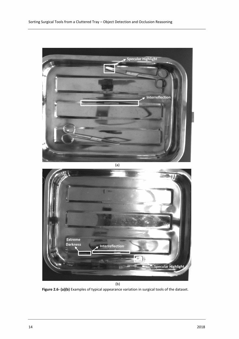
All the methods and algorithms presented so far in this dissertation are applied in
random bin picking of industrial parts, however not all can be applied to objects made by
non-Lambertian materials (e.g. metal, ceramic or glass) such as surgical instruments, which
are prone to display an unpredictable change in intensity throughout the object, as shown in
Figure 2.6 that contains images used in this dissertation.
2.8.1. External Markers
A common approach to avoid surgical tool detection errors is the addition of external
markers to the surgical tool which significantly eases the recognition task. Over the years
several studies resorted this approach, using a variety of external markers such as
recognizable patterns [101], color tags [102], light-emitting diodes [103], RFID tags [10]
and 2D data matrix barcodes [3][104][105].
The work of Xu et al. [104][105] is of great interest due to the high success rate
achieved. They used Key Surgical®KeyDot to identify the tools through a 2D data matrix.
The corners of the code are used to compute an affine transformation that aligns a template
to the real instrument, in order to obtain a virtual map of the scene, as the one present in
Figure 2.7, to apply the occlusion reasoning.
Sorting Surgical Tools from a Cluttered Tray – Object Detection and Occlusion Reasoning
14 2018
Specular Highlight
Interreflection
(a)
Specular Highlight
Interreflection
Extreme Darkness
(b) Figure 2.6- (a)(b) Examples of typical appearance variation in surgical tools of the dataset.

STATE OF ART
Diana Martins Lavado 15
Although these methods show great potential, they have a huge drawback, which is
that they all apply physical modifications to surgical tools that might violate regulations,
raise safety concerns and, therefore hampering their implementation on surgical instruments.
2.8.2. Marker-Less Approaches
In 2017, Bouget et al. [106] published a literature review of marker-less approaches
for the detection and tracking of surgical tools and an adapted summary table could be found
in Table 2.1.
However, there are a wide range of studies and methodologies that were not
addressed. Carpintero et al. [8][107] resorted to Matrox Imaging Library (MIL) Finder Tool
to extract the instrument models, and to recognize the surgical tools in the scene. Other
approaches involved the approximation of the surgical instruments to geometric shapes such
as tubular shapes [47], [108] or pointy solid cylinders [109], [110], [84]. In 2017, Li et al.
[111] uses two cameras and performs blob analysis to extract the surgical instruments from
the background obtaining surgical instruments model (SIM) through stereo vision, thus
extracting point-pair features from SIM to distinguish the tools.
In 2016, M2CAI released a challenge in which the goal was to detect specific
surgical tools from the m2cai16-tool dataset. Most of the network architectures of top
winning deep learning approaches were modifications of AlexNet: Twinanda et al. [112]
Figure 2.7- Pose estimation using the four corners of the data matrices from both template and input image of the container after non-linear refinement [104].

Sorting Surgical Tools from a Cluttered Tray – Object Detection and Occlusion Reasoning
16 2018
achieved 52,5% mAP (mean Average Precision) by developing ToolNet and EndoNet,
followed by Sahu et al. [113][114] with 53,9% mAP and 65% mAP respectively. Another
approach was proposed by Raju[115] which combined VGGNet with GoogLeNet obtaining
63,7% mAP, that was surpassed by Choi et al. [116] who made some modifications to YOLO
such as the addition of one fully connected layer, dropout, and batch normalization, thus
pretraining the convolutional layers on ImageNet 1000-class dataset achieving a total of
72,26% mAP.
The highest success rates for detecting surgical instruments are 87,6% mAP and
95,81% AUC (Area Under the ROC Curve) achieved by Hossain et al. [117] and Prellberg
et al. [118] respectively in 2018. The network architecture of Hossain et al. is a combination
of VGG-16 and RPN (Region Proposal Network), whereas the one developed by Prellber et
al. was built upon a 50 layer ResNet.

STATE OF ART
Diana Martins Lavado 17
Table 2.1- Summarized literature review of marker-less approaches for surgical tools detection and tracking. Table adapted from [106].
Features Prior knowledge Traking
Co
lor
Gra
die
nts
HO
G
Tex
ture
Sh
ape
Mo
tio
n
Dep
th
Sem
anti
c
Lab
els
To
ol
shap
e
To
ol
loca
tio
n
Use
r as
sist
.
Kin
emat
ics
Bay
es.
Par
ticl
e
Init
iali
sati
on
(Allan et al., 2013) [84] ✓ ✓ ✓ ✓ ✓
(Allan et al., 2014) [119] ✓ ✓ ✓ ✓ ✓ ✓ ✓ ✓
(Allan et al., 2015) [120] ✓ ✓ ✓ ✓ ✓ ✓ ✓ ✓
(Alsheakhali et al., 2015) [121] ✓ ✓ ✓
(Bouget et al., 2015) [122] ✓ ✓ ✓ ✓
(Cano et al., 2008) [123] ✓ ✓ ✓ ✓ ✓
(Charrière et al., 2017) [124] ✓ ✓ ✓ ✓
(Doignon et al., 2005) [125] ✓ ✓ ✓ ✓ ✓
(Doignon et al., 2007) [126] ✓ ✓ ✓
(Haase et al., 2013) [110] ✓ ✓ ✓ ✓ ✓
(Kumar et al., 2013) [127] ✓ ✓ ✓ ✓
(McKenna et al., 2005) [128] ✓ ✓ ✓ ✓ ✓
(Pezzementi et al., 2009) [129] ✓ ✓ ✓
(Reiter & Allen, 2010) [130] ✓ ✓ ✓ ✓ ✓
(Reiter et al., 2012) [131] ✓ ✓ ✓ ✓
(Reiter et al., 2012) [132] ✓ ✓ ✓ ✓ ✓ ✓ ✓
(Richa et al., 2012) [133] ✓ ✓
(Rieke et al., 2015) [134] ✓ ✓ ✓ ✓
(Speidel et al., 2006) [135] ✓ ✓ ✓
(Speidel et al., 2008) [108] ✓ ✓ ✓ ✓
(Speidel et al., 2014) [136] ✓ ✓ ✓ ✓ ✓
(Sznitman et al., 2014) [47] ✓ ✓ ✓
(Voros et al., 2007) [137] ✓ ✓ ✓ ✓
(Wolf et al., 2011) [138] ✓ ✓ ✓ ✓ ✓
(Zhou & Payandeh, 2014)[139] ✓ ✓ ✓

Sorting Surgical Tools from a Cluttered Tray – Object Detection and Occlusion Reasoning
18 2018

Diana Martins Lavado 19
3. INSTRUMENTS AND SOFTWARE
The aim of this dissertation was to develop a successful methodology for detecting
surgical tools and perform occlusion reasoning to be applied on a system, that would sort the
surgical tools from a cluttered tray after disinfection to assembly surgical kits.
The first step towards accomplishing that goal is to choose the surgical instruments,
therefore, with the intention of making the system useful and as close to the “real world” as
possible, the Chief Nurse of the Main Operating Room of the Hospital of University of
Coimbra, Jorge Tavares, was interviewed and promptly supplied lists of surgical kits
amongst a wide range of medical specialties. These lists were analyzed and it was chosen
the most popular instruments across several medical fields, however, due to some difficulties
in acquiring those surgical tools, the instruments used throughout this research were the ones
found which had the closest form to the intended tools, which are: Scalpel nº4, Straight
Dissection Clamp, Straight Mayo Scissor and Curved Mayo Scissor.
The camera used for this project was the Teledyne Dalsa BOA INS, which has
640x480 of pixel resolution. However, despite being a smart camera, none of its
functionalities were used.
The object detection, as well as occlusion reasoning stage in this dissertation, was
accomplished by resorting to convolutional neural networks as will be further explained.
These neural networks were trained on the operating system Ubuntu 16.04 on dual boot
because, at the time, the NVIDIA CUDA toolkit for Windows was incompatible with
Microsoft Visual Studio 2015. An installation script of all the required software and
packages to train the neural networks on Ubuntu can be found on ANNEX A.
Independently of the operating system, the required software for the execution of this
project are:
• CUDA 9.1, which is a parallel computing platform by NVIDIA and it is
used with the intention of speeding up the running time;
• CuDNN 7.0.5, that was also developed by NVIDIA and is a GPU-
accelerated library of primitives for deep neural networks and it is used

Sorting Surgical Tools from a Cluttered Tray – Object Detection and Occlusion Reasoning
20 2018
with the aim of speeding up the training and implementation of the deep
neural networks;
• OpenCV 3.4.0, which stands for Open Source Computer Vision Library
is compatible with C++, python, and java, being supported by Windows,
Linux, Mac OS, iOS and Android. It can also be compiled with OpenCL
using the full capabilities of the hardware for acceleration purposes
• Darknet is an open source neural network framework written in C and
CUDA which supports CPU and GPU computation. The original pjreddie
repository only works on Ubuntu whereas the AlexeyAB darknet
repository is compatible with Windows and Ubuntu. Both darknet
frameworks can be compiled enabling CuDNN, OpenCV, OpenMP, and
GPU on the makefile.
It is very important to install the software and libraries with the order that were listed
above, due to dependencies during their installation. Another aspect that requires attention
are version compatibilities, because whenever a software undergoes updates it is likely that
it no longer is compatible with some of the other software or libraries mentioned and while
the other programs are being developed to support the improvement, the most recent releases
are not compatible, which proofs the utter importance of version compatibility.
Regarding the hardware, two computers were used: one for training the neural
networks and other for developing the application and perform the train and test group split
of the data as well as analyze the results and their respective hardware specification could
be found on Table 3.1.
Table 3.1- Hardware specifications.
Neural Networks Training App development
Graphics Card NVIDIA GEFORCE GTX 1050Ti NVIDIA GEFORCE GTX 850M
Dedicated memory 4GB 4GB

Diana Martins Lavado 21
4. CLASSICAL APPROACH
The aim of this project was to develop a robust detection system able to handle
occlusion for sorting surgical tools assessing the first tool to be removed and returning the
grasping point coordinates which do not require great precision due to the use of an
electromagnetic gripper. However, this dissertation focus mainly on object detection and
occlusion reasoning.
Due to the objective of recognizing the tool the as fastest as possible, the initial
approach to achieve the surgical object detection and sorting was similar to studies from Xu
et al. [3][104][105] and its scheme is presented in Figure 4.1. Despite the final developed
approach in this dissertation is not the one described in this chapter, it still is an important
contribution to solve random bin-picking of surgical tools.
Figure 4.1- Scheme of all the steps involved in this project.

Sorting Surgical Tools from a Cluttered Tray – Object Detection and Occlusion Reasoning
22 2018
Detection and Classification
The tool’s class ID is encoded into a 2D data matrix barcode, which besides
making the identification task quite straightforward, it eases the pose estimation through
computing an affine transformation between the four corners of the matrix of the template
and the real object. The detection and classification of the tools in the tray was planned to
be achieved using the software package 2DTG, that is capable of decoding multiple small
codes present in an image and return the position of all their corners.
Virtual Occupancy Map
After finding the position and classification of the tools in the tray, an occupancy
map would be built by applying an affine transformation on the instrument template before
adding it to the map with the respective position and orientation, thus a non-linear refinement
would be implemented to improve the alignment of the templates with the surgical
instruments in the scene.
Occlusion Reasoning
In order to determine the tool to be first removed it is mandatory to overcome
the difficulties imposed by occlusion. Thus, each instrument template is assigned to one bit
in the occupancy map which is a single channel image. Then each pixel would be analyzed
and its intensity value assessed accordingly. For example, if bit 4 is 1 then the instrument D
is there, however, if the bit 2 is 0 then instrument B is absent. This reasoning may provide a
location where an occlusion occurs (when the same pixel has more than one bit assigned),
and by comparing the several hypotheses (A occludes B or B occludes A) with the real image
it would be possible to determine which tool is on top of the tray and therefore, the first to
be removed.
Pose Estimation and Kits Assembly
The electrical current, position, and orientation of an electromagnetic gripper
would be adjusted accordingly to the shape, mass, material and touch point of the tool to be
removed. After picking up the surgical instrument, the robot would place it onto the proper
location, in accordance to the surgical kit being set up.

Diana Martins Lavado 23
4.1. Templates
In this approach, the first step towards pose estimation is the creation of a
template for each surgical instrument class, noting that the same tool could have more than
one template if it has more than one possible face, requiring a different barcode for every
single one.
There are three main image segmentation approaches to obtain the templates:
edge-based, threshold-based and region-based. The next sections of this dissertation make
an overview of some of these methods and their implementation in surgical tools, showing
their application in the original Figure 4.2. All the templates were built in C++ through
Microsoft Visual resorting to the OpenCV library.
4.1.1. Edge-based Image Segmentation
The first edge detector implemented was Sobel [11] which is a discrete
differentiation operator combining both Gaussian smoothing and differentiation. It
calculates an approximation of the gradient of an image intensity function, by convolving
the image, I, with a specific filter. From the Sobel operator, two derivatives are computed
Figure 4.2- Original image of a Curved Mayo Scissor.
Sorting Surgical Tools from a Cluttered Tray – Object Detection and Occlusion Reasoning
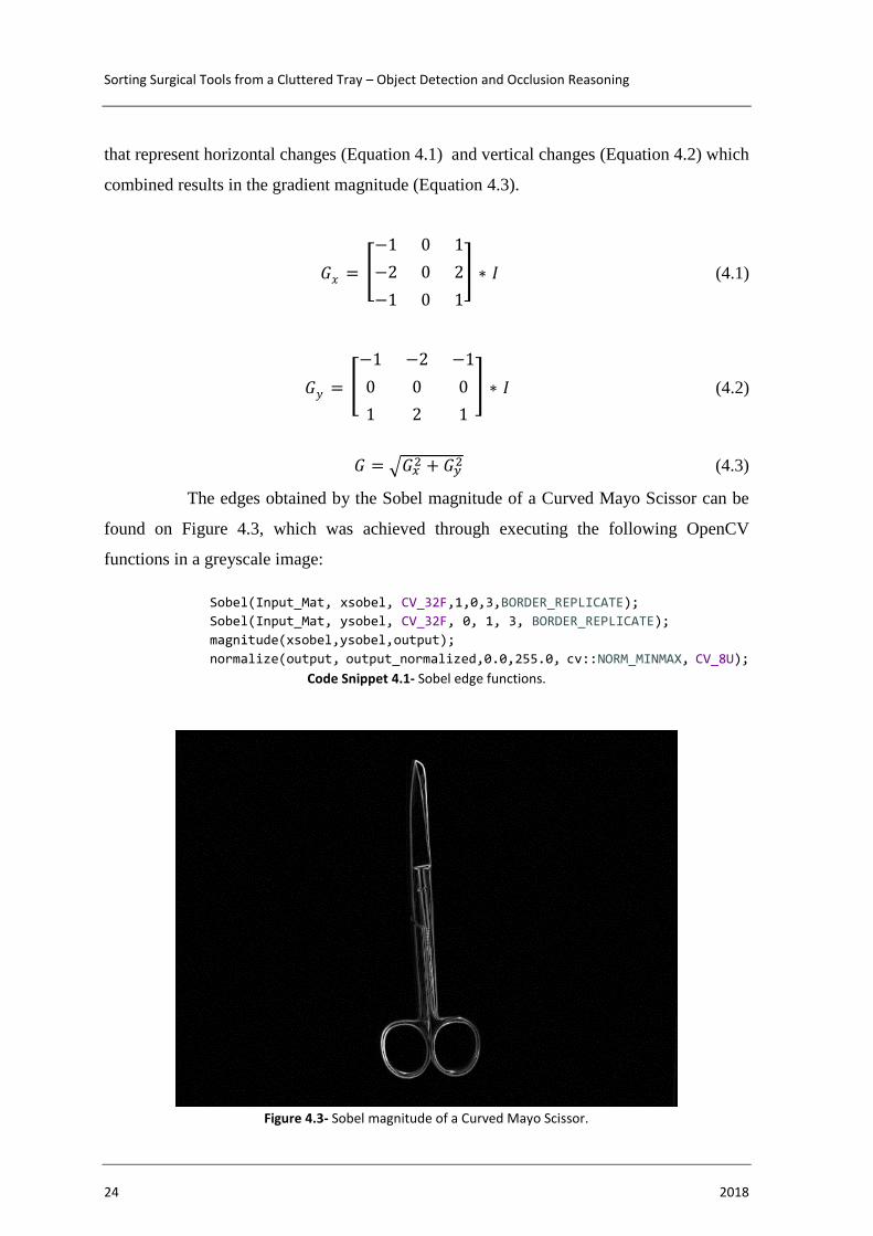
24 2018
that represent horizontal changes (Equation 4.1) and vertical changes (Equation 4.2) which
combined results in the gradient magnitude (Equation 4.3).
𝐺𝑥 = [−1 0 1
−2 0 2
−1 0 1
] ∗ 𝐼 (4.1)
𝐺𝑦 = [−1 −2 −1
0 0 0
1 2 1
] ∗ 𝐼 (4.2)
𝐺 = √𝐺𝑥2 + 𝐺𝑦2 (4.3)
The edges obtained by the Sobel magnitude of a Curved Mayo Scissor can be
found on Figure 4.3, which was achieved through executing the following OpenCV
functions in a greyscale image:
Sobel(Input_Mat, xsobel, CV_32F,1,0,3,BORDER_REPLICATE);
Sobel(Input_Mat, ysobel, CV_32F, 0, 1, 3, BORDER_REPLICATE); magnitude(xsobel,ysobel,output);
normalize(output, output_normalized,0.0,255.0, cv::NORM_MINMAX, CV_8U); Code Snippet 4.1- Sobel edge functions.
Figure 4.3- Sobel magnitude of a Curved Mayo Scissor.

Diana Martins Lavado 25
According to the OpenCV Sobel documentation, this operator can produce some
noticeable inaccuracies, which can be reduced by the Scharr operator (Equations 4.4, 4.5,
4.3) that minimizes the angular error in Fourier Transform domain. However, such
improvement was not corroborated by Figure 4.4, that is very similar to Figure 4.3.
𝐺𝑥 = [−3 0 3
−10 0 10
−3 0 3
] ∗ 𝐼 (4.4)
𝐺𝑦 = [−3 10 3
0 0 0
3 10 3
] ∗ 𝐼 (4.5)
Nevertheless, these edge operators are sensitive to noise and do not work as well
in smooth edges, as verified in Figure 4.5, in which was applied the gaussian blur function
with a 3x3 kernel and an x and y standard deviation of 50 before the implementation of the
edge operators.
Figure 4.4- Scharr magnitude image of a Curved Mayo Scissor.

Sorting Surgical Tools from a Cluttered Tray – Object Detection and Occlusion Reasoning
26 2018
A more suitable algorithm for image segmentation through edge detection was
proposed by John Canny [12] and had the following main steps:
• Apply smoothing derivatives to suppress noise;
• Apply a high threshold to detect strong edge pixels;
• Link those pixels to form strong edges;
• Apply a low threshold to find weak but plausible edge pixels;
• Extend the strong edges to follow weak edge pixels.
In order to manually find the best set of thresholds, it was developed an
application with a sliding bar, which whenever moved callbacks the OpenCV Canny
function with the new parameters chosen, which can be observed in Figure 4.6 as well as the
best parameters applicable to the Curved Mayo Scissor.
Additionally, it is possible to obtain the contours of the surgical tool from the
edges, as shown in Figure 4.7. This can be computed through the functions present in Code
Snippet 4.2, in which “edges” is the output Mat from the Canny function, “contours” is a
vector with information of the lines (vector of points) and “drawing” is the output Mat with
the all the image contours. The code present is also within the callback function previously
mentioned, in order to observe the impact in both edge and contour image, while changing
each threshold value.
(a) (b)
Figure 4.5- Edge operators implementation on a smoothed image. (a) Sobel (b) Scharr.

Diana Martins Lavado 27
(a)
(b)
Figure 4.6- (a) Sliding bar in original image of a Curved Mayo Scissor (b) Canny edges with threshold values presented in sliding bar.

Sorting Surgical Tools from a Cluttered Tray – Object Detection and Occlusion Reasoning
28 2018
GaussianBlur(Input_Mat, blured, Size(9, 9), 1, 1, BORDER_REPLICATE);
findContours(edges, contours,hierarchy, RETR_TREE, CHAIN_APPROX_SIMPLE,
Point(0, 0));
drawContours(drawing, contours, index_color, color, 2, 8, hierarchy, 0,
Point());
Code Snippet 4.2- Object contour from Canny edges.
4.1.2. Threshold-based Image Segmentation
Other approaches for image segmentation are threshold-based techniques, which
compare the intensity levels with a threshold, that can be automatically found through Otsu’s
method. This method assumes that the image contains two classes of pixels (foreground and
background pixels), meaning that the grayscale image is converted to a binary image, then
some noise is removed by erosion and finally, is found the threshold that minimizes the
weighted within-class variance, which is equivalent to maximizing the variance between
classes.
Figure 4.7- Contours of Curved Mayo Scissor controlled with the sliding bar application.

Diana Martins Lavado 29
The resultant image segmentation of a Curved Mayo Scissor is displayed in
Figure 4.8, and the respective OpenCV function is in Code Snippet 4.3.
threshold(Input_Mat, Binary, thresh, thresh2, CV_THRESH_OTSU);
Code Snippet 4.3- Image segmentation using Otsu’s method
4.1.3. Region-based Image Segmentation
These type of approaches merge and split pixels into sub-regions, considering
grayscale intensity values similarity with neighboring pixels. One of these methods is the
watershed algorithm [140], which quoting the OpenCV documentation “any grayscale image
can be viewed as a topographic surface where high intensity denotes peaks and hills while
low intensity denotes valleys. You start filling every isolated valleys (local minima) with
different colored water (labels). As the water rises, depending on the peaks (gradients)
nearby, water from different valleys, obviously with different colors will start to merge. To
avoid that, you build barriers in the locations where water merges. You continue the work
of filling water and building barriers until all the peaks are under water. Then the barriers
you created gives you the segmentation result” [141].
Figure 4.8- Image segmentation of a Curved Mayo Scissor resorting to Otsu’s method.

Sorting Surgical Tools from a Cluttered Tray – Object Detection and Occlusion Reasoning
30 2018
In order to improve the segmentation of an image through the watershed
algorithm, all the background pixels should have intensity values of 0 (black), because it
eases the discrimination of foreground pixels while applying the Distance Transform.
Afterward, it is advised to implement a Laplacian filter to sharpen the image, however, it
was verified that this results in an overly sectioned image of the surgical tools and that a
smoothing filter (e.g. Gaussian) leads to a more accurate segmentation. The next step is to
create a binary image resorting to Otsu’s method and apply the distance transform whose
output is displayed in Figure 4.9, whose peaks are going to be extracted by applying a
threshold and a morphologic operation (dilation). Then, the OpenCV function findcontours
allows to create markers for the watershed, that are posteriorly drawn and filled with random
colors. Some of the C++ lines of this algorithm could be found on Code Snippet 4.4. and the
final result in Figure 4.10.
GaussianBlur(Input_Mat, img, Size(5, 5), 1, 1, BORDER_REPLICATE);
cvtColor(img, imgResult, CV_BGR2GRAY); threshold(imgResult, imgResult, 66, 300, CV_THRESH_BINARY |
CV_THRESH_OTSU);
distanceTransform(imgResult, dist_transf, CV_DIST_L2, 3);
normalize(dist_transf, dist_transf, 0, 1., NORM_MINMAX); threshold(dist_transf, dist_transf, .4, 1., CV_THRESH_BINARY);
Mat kernel1 = Mat::ones(3, 3, CV_8UC1);
dilate(dist_transf, dist_transf, kernel1); dist_transf.convertTo(dist_transf8u, CV_8U);
findContours(dist_transf8u, contours2, CV_RETR_EXTERNAL,
CV_CHAIN_APPROX_SIMPLE);
drawContours(markers, contours2, static_cast<int>(i),
Scalar::all(static_cast<int>(i) + 1), -1);
circle(markers, Point(5, 5), 3, CV_RGB(255, 255, 255), -1);
watershed(image1, markers);
markers.convertTo(mark, CV_8UC1);
bitwise_not(mark, mark); Code Snippet 4.4- Main lines of code of the watershed algorithm
At this point in the development of dissertation we were still unable to acquire a
license for the 2DTG software, which would allow to decode multiple 2D data matrix
barcodes in the same image and also the camera used in this project had a pixel resolution
of 640x480, which was not enough to identify the smallest change within the barcodes, due
to their reduced size. Therefore, this approach to detect surgical tools became unsuitable and

Diana Martins Lavado 31
it was required to follow a completely new path towards the bin-picking of surgical tools in
a clustered tray, which is discussed in Chapter 5.
Figure 4.9- Distance Transform of a Curved Mayo Scissor.
Figure 4.10- Watershed segmentation of a Curved Mayo Scissor.

Sorting Surgical Tools from a Cluttered Tray – Object Detection and Occlusion Reasoning
32 2018

Diana Martins Lavado 33
5. MODERN APPROACH
Within the last few years, Convolutional Neural Networks have undergone an
upsurge solving problems in a wide range of fields such as object detection in which the
most relevant networks are Faster R-CNN [91], SSD [99], YOLO(that currently has three
versions) [96], [97], [98].
According to Huang et al. [142], which compares the accuracy of Faster R-CNN,
R-FCN and SSD meta-architectures throughout several datasets and feature extractors, the
Faster R-CNN obtains better results in comparison with SSD, as shown in Figure 5.1, despite
the higher memory allocation, training duration and detection time.
According to a graph presented in YOLO v2 paper, which is displayed in Figure 5.2,
the Faster R-CNN Resnet evidences the highest mAP, followed by YOLOv2 and SSD
respectively, considering that the camera resolution is 640x480 pixels. However, in order to
enable real-time applications it is preferable to choose a network architecture able to detect
around 60 frames per second (FPS) at the cost of a slightly lower mAP. Hence, the neural
network used in this dissertation was YOLOv2.
Figure 5.1- Accuracy of detector (mAP on COCO) vs accuracy of feature extractor (on ImageNet-CLS) of the low resolution models [142].

Sorting Surgical Tools from a Cluttered Tray – Object Detection and Occlusion Reasoning
34 2018
The current object detector neural network state of art is YOLOv3 [98] and, although
it was only published in March of 2018, it was also implemented for object detection in the
final stages of this dissertation.
5.1. YOLO v2
YOLO stands for “you only look once” and is a real-time object detection system
which was firstly introduced in 2015 [96], having undergone enhancements over time
resulting into three versions.
The second version of YOLO [97] is considered a single shot detector that splits the
image into an SxS grid, and each grid cell is responsible for predicting a fixed number of
randomly sized boundary boxes, B, each with one box confidence score and one object
classification, C, per grid cell, as shown in Figure 5.3. These predictions are then encoded
by a 𝑆 × 𝑆 × (𝐵 ∗ 5 + 𝐶) tensor, which in this dissertation corresponds to 7x7x14.
Figure 5.2- Accuracy and speed comparison on VOC 2007 dataset [97].

Diana Martins Lavado 35
The YOLOv2 architecture used on this project is represented in Figure 5.4, showing
19 convolutional layers, 5 max-pooling layers and a passthrough layer to enable the use of
fine grain features, which lead to a mAP of 78,6% on VOC dataset.
In comparison with YOLO, the second version of this neural network has an
improved performance due to four main factors:
• Batch normalization, which is implemented at the end of every convolutional
layer aiding the model to converge and stabilize, reducing overfitting and,
thus leading to the removal of the dropout layer;
• High resolution classifier: the network was pretrained on ImageNet dataset
and then was resized (to higher resolution) and fine-tuned for classification,
instead of just resizing it for detection, which was the approach implemented
on YOLOv1;
• Dimension clusters, which are the result of applying K-mean clustering to the
bounding boxes in training data, instead of resorting to predefined anchor
boxes (like YOLOv1);
• Multiscale-training: during training the network randomly changes the
images size
Figure 5.3- YOLO system model detector as a regression problem [96].

Sorting Surgical Tools from a Cluttered Tray – Object Detection and Occlusion Reasoning
36 2018
The third version was not tested on the VOC dataset yet, however it is possible to
compare the performance of the two latest versions of YOLO on the COCO dataset, in which
the mAP is 44% for YOLOv2 and 57,9% for YOLOv3. Since the implementation of
YOLOv3 was also tested at the end of this dissertation, it is important to explain the main
improvements in comparison to YOLOv2, which are the following:
• Bounding box predictions: it also uses dimension clusters with resemblance
of the previous version, however predicts the objectiveness score using
logistic regression;
• Class predictions: for each class it is used logistic classifiers, whereas
YOLOv2 implements a regular softmax layer;
• Predictions across scales: the bounding boxes are predicted with 3 different
scales to make the detector robust to vary object scales;
• Feature extractor: instead of using darknet-19 as a backbone, YOLOv3 uses
darknet-53, which has 53 convolutional layers and is more efficient than
ResNet-101.
5.2. Dataset
Most of the public datasets used for surgical tools detection were obtain from in-
vivo surgery videos, for example:
• From DaVinci surgery [127];
• From retinal and laparoscopic videos [143];
• From minimally-invasive surgery [84];
• From robotic-assisted minimally-invasive surgery procedures taking scale
and rotation into account [144];
• From brain and spine tumor removal procedures [122];
• From gallbladder excision surgery [116];
• From cataract surgery videos [118];
• From cholecystectomy procedures, the m2cai16-tool dataset [115].

Diana Martins Lavado 37
Image
Convolutional
Maxpool
Convolutional
Maxpool
3 Convolutional
Maxpool
3 Convolutional
Maxpool
5 Convolutional
Maxpool
5 Convolutional
5 Convolutional
112x112
56x56
28x28
14x14
7x7
7x7
7x7
Figure 5.4- YOLO v2 architecture.

Sorting Surgical Tools from a Cluttered Tray – Object Detection and Occlusion Reasoning
38 2018
However, the datasets mentioned above lack in data, diversity, precision in
annotations and do not contain data regarding the surgical tools used in this dissertation.
Therefore, a new dataset was built with custom data.
The first step towards the dataset assembly was to take a lot of photos of each surgical
instrument individually on a surgical tray with several rotations, inclinations and lightening
conditions throughout the tray, resorting to iNspect Express (camera software) from
Teledyne. Afterwards, in order to make the method robust to occlusion, each tool is paired
with another of different class and the process is repeated, under the same conditions
previously described, with one of the instruments occluding the other and vice versa. Finally,
another set of photos are taken with tools of all classes without occlusion. The total amount
of pictures is discriminated in Table 5.1 in which the instruments with a “+” before their
name are on top of previous individually class.
Table 5.1- Discrimination of the amount of pictures in the dataset.
In machine leaning, the bigger the dataset the more accuracy the model is going to
achieve, especially in DL, which requires a higher amount of data [145]. There are a wide
range of techniques to perform data augmentation of an existing dataset, such as cropping,
rotating, flipping and scaling input image. In this dissertation, the data augmentation was
Surgical tools present in the image Amount
of photos
Scalpel nº4 (individually) 550
+ Straight Dissection Clamp 71
+ Straight Mayo Scissor 49
+ Curved Mayo Scissor 64
Straight Dissection Clamp (individually) 460
+ Scalpel nº4 64
+ Straight Mayo Scissor 76
+ Curved Mayo Scissor 80
Straight Mayo Scissor (individually) 450
+ Scalpel nº4 59
+ Straight Dissection Clamp 77
+ Curved Mayo Scissor 79
Curved Mayo Scissor (individually) 550
+ Scalpel nº4 69
+ Straight Dissection Clamp 117
+ Straight Mayo Scissor 70
All Classes 100

Diana Martins Lavado 39
implemented by defining “random=1” in the network configuration on darknet, which during
training is responsible by randomly resizing the network to a size between 320x320 and
608x608 (multiples of 32) for every 10 iterations as well as changing color (hue, saturation
and exposure) and randomly cropping (through jitter of edges).
The dataset built was published on Kaggle with the title “Labeled Surgical Tools and
Images” achieving around 600 views in 20 days.
5.2.1. Labeling
YOLOv2 is used in this dissertation as a supervised learning algorithm therefore, it
requires the bounding boxes coordinates and corresponding label of all the objects present
in each image which needs to be written in a text file with the same name as the respective
image. Two different programs were tested in order to perform image labeling: BBox-Label-
Tool and Yolo_mark.
5.2.1.1. BBox-Label-Tool
This is a python program [146] compatible with both Windows and Ubuntu, requiring
python 2.7 and the PIL(pillow) package. In order to function the images have to be divided
by class and placed in the folders “…/Images/001”, “…/Images/002” and so on, thus it is
important to mention that the folder “…/Examples” need to contain the same subfolders than
“…/Images”.
Other requirements are that image names cannot contain “.”, which can be modified
by “Bulk Rename Utility” and all images must have a jpeg format which can be achieved by
“Bulk Converter” software or by typing “ren *.bmp *.jpeg” at the image folder terminal.
By the time it was used for the dissertation, this labeling tool did not supported multi
class labeling (objects from different classes in the same image), so the solution would be to
change the class if of all labels and concatenate the text files referent to the same image or
resort to Yolo_mark labeling tool instead, which is described in section 5.2.1.2. However, in
the meanwhile, a branch of BBox-Label-Tool supporting multiclass objects was developed
[147].

Sorting Surgical Tools from a Cluttered Tray – Object Detection and Occlusion Reasoning
40 2018
5.2.1.2. YoloMark
With resemblance to the previous tool, Yolo_mark [148] is also able to support both
Windows and Ubuntu requiring images with the .jpg format as well.
Since the training of the neural network would be done in Ubuntu, the same operating
system was used for image labeling. Thus, two text files are required: one with all the image
paths and other with the different class names.
The Figure 5.6 shows the labeling GUI that is created whenever the command
“./yolo_mark images_folder_path image_list_path names_path” is typed onto the terminal.
The output of this tool is a text file per image, containing in each line the class
number, x, y, width and height of a bounding box label, in which x and y are the coordinates
of the center of the rectangle (and not the left corner as in BBox-Label-Tool)). The content
of an example label file could be found on Figure 5.7 that represents the labels of the surgical
tools displayed on Figure 5.6.
Besides the detection challenge, YOLOv2 was also used to overcome occlusion
classifying each tool after detection as top (not occluded) or bottom (occluded) easing the
decision regarding which instrument should be firstly removed. Hence the need for labeling
not only for the surgical tool classification but whether it is on top or bottom as well. Since
Figure 5.5- GUI of BBox-Label-Tool.

Diana Martins Lavado 41
the bounding boxes of the labels for occlusion handling remain the same, a python script
was developed in order to change the class number of each label, which was only possible
due to the previous knowledge on which tool was on top in specific intervals of images.
Figure 5.6- Yolo_mark graphical user interface.
Figure 5.7- Label file example of the image present in Figure 5.6.
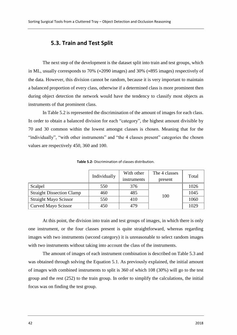
Sorting Surgical Tools from a Cluttered Tray – Object Detection and Occlusion Reasoning
42 2018
5.3. Train and Test Split
The next step of the development is the dataset split into train and test groups, which
in ML, usually corresponds to 70% (≈2090 images) and 30% (≈895 images) respectively of
the data. However, this division cannot be random, because it is very important to maintain
a balanced proportion of every class, otherwise if a determined class is more prominent then
during object detection the network would have the tendency to classify most objects as
instruments of that prominent class.
In Table 5.2 is represented the discrimination of the amount of images for each class.
In order to obtain a balanced division for each “category”, the highest amount divisible by
70 and 30 common within the lowest amongst classes is chosen. Meaning that for the
“individually”, “with other instruments” and “the 4 classes present” categories the chosen
values are respectively 450, 360 and 100.
Table 5.2- Discrimination of classes distribution.
At this point, the division into train and test groups of images, in which there is only
one instrument, or the four classes present is quite straightforward, whereas regarding
images with two instruments (second category) it is unreasonable to select random images
with two instruments without taking into account the class of the instruments.
The amount of images of each instrument combination is described on Table 5.3 and
was obtained through solving the Equation 5.1. As previously explained, the initial amount
of images with combined instruments to split is 360 of which 108 (30%) will go to the test
group and the rest (252) to the train group. In order to simplify the calculations, the initial
focus was on finding the test group.
Individually With other
instruments
The 4 classes
present Total
Scalpel 550 376
100
1026
Straight Dissection Clamp 460 485 1045
Straight Mayo Scissor 550 410 1060
Curved Mayo Scissor 450 479 1029

Diana Martins Lavado 43
Table 5.3- Discrimination of images with combination of instruments in the train and test groups
{
108 = 𝑐1 + 𝑠𝑠1 + 𝑐𝑠1 + 𝑠1 + 𝑠2 + 𝑠3
108 = 𝑠1 + 𝑠𝑠2 + 𝑐𝑠2 + 𝑐1 + 𝑐2 + 𝑐3
108 = 𝑠2 + 𝑐2 + 𝑐𝑠3 + 𝑠𝑠1 + 𝑠𝑠2 + 𝑠𝑠3
108 = 𝑠3 + 𝑐3 + 𝑠𝑠3 + 𝑐𝑠1 + 𝑐𝑠2 + 𝑐𝑠3𝑐1 + 𝑠𝑠1 + 𝑐𝑠1 = 𝑠1 + 𝑠𝑠2 + 𝑐𝑠2
𝑠1 + 𝑠𝑠2 + 𝑐𝑠2 = 𝑠2 + 𝑐2 + 𝑐𝑠3
𝑠2 + 𝑐2 + 𝑐𝑠3 = 𝑠3 + 𝑐3 + 𝑠𝑠3
𝑐𝑠3 = 𝑠𝑠3
𝑠𝑠1 = 5
𝑐𝑠1 = 25
𝑠1 = 10
𝑠2 = 14
(5.1)
variable Train Test
Scalpel nº4 - 315 135
+ Straight Dissection Clamp c1 46 24
+ Straight Mayo Scissor ss1 44 5
+ Curved Mayo Scissor cs1 36 25
Straight Dissection Clamp - 315 135
+ Scalpel nº4 s1 54 10
+ Straight Mayo Scissor ss2 32 32
+ Curved Mayo Scissor cs2 40 12
Straight Mayo Scissor - 315 135
+ Scalpel nº4 s2 46 14
+ Straight Dissection Clamp c2 30 23
+ Curved Mayo Scissor cs3 50 17
Curved Mayo Scissor - 315 135
+ Scalpel nº4 s3 26 30
+ Straight Dissection Clamp c3 50 7
+ Straight Mayo Scissor ss3 50 17
All 4 classes present - 70 30
Total 1834 786

Sorting Surgical Tools from a Cluttered Tray – Object Detection and Occlusion Reasoning
44 2018
The first 4 equations translate that the sum of all images with a determined instrument
must be equal to 108, and the following 3 equations are meant to balance the amount of times
a determined tool is occluded (on the bottom), which is important for the training of the
networks handling occlusion. The last parameters were necessary so that the equation system
would be solvable, and their values were a mixture between intuition and trial and error to
achieve the best results.
The values for the train group were obtained by subtracting the same variables of
the test group to the values presented in Table 5.2.
Therefore, a python script was developed, in which for each “category” it would
randomly sort 5 times all the possible options and the first x (x being the corresponding value
in Table 5.3 on the test group ) would be added to the test file and the following y (y being
the corresponding value in Table 5.3 on the train group) would be added to the train file.
In Figure 5.8 are displayed two chord diagrams showing the relative amount of
images for each combination of instruments in both train (Figure 5.8(a)) and test (Figure
5.8(b)) groups. The ribbons (each connection) thickness represents the relative amount of
images in which the two instruments it connects are present in the same image. Whenever it
does not have a ribbon, it symbolizes the amount of images in which that instrument appear
individually. Therefore, from the analysis of the diagrams, it is possible to conclude that both
train and test groups are balanced, because in each graph the ribbons have approximately the
same thickness, although in the test group straight mayo scissor + straight dissection clamp
and curved mayo scissor + scalpel evidences a slightly lower amount of images than the
other combinations.
Regarding the occlusion reasoning, initially the data split into train and test groups
was the same only changing the labels, however, as will be explained in Section 5.4.1.1, it
was necessary to train an occlusion handling network per surgical tool class, which requires
a different division of the data. Since the dataset relative to occlusions is very unbalanced,
due to the largely higher amount of images with the tools on top rather than occluded,
therefore all of the data of each instrument class is randomly sorted 5 times and afterwards
de the first x (x being 30% of the respective total value presented in Table 5.2) will belong
to the test group for the occlusion reasoning of that object and the rest of the image goes to
the train group.
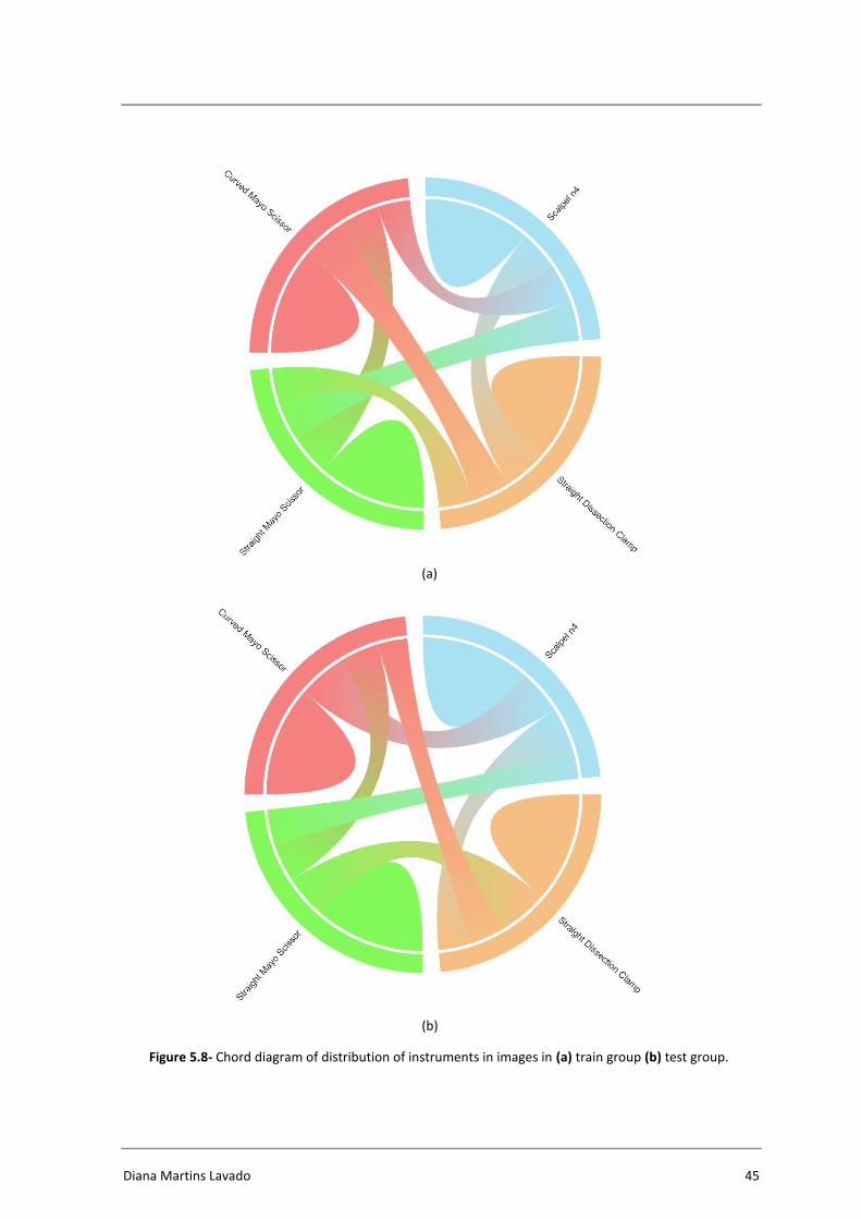
Diana Martins Lavado 45
(a)
(b)
Figure 5.8- Chord diagram of distribution of instruments in images in (a) train group (b) test group.

Sorting Surgical Tools from a Cluttered Tray – Object Detection and Occlusion Reasoning
46 2018
5.3.1. Cross-Validation
The purpose of test group is to estimate the model performance on unseen data,
although YOLOv2 uses this group as a validation helping to adjust some hyperparameters,
it never actually “learns” from it. However, it is important to evaluate the stability and
accuracy of the neural network, which is achieved by cross-validation, that is a method
responsible for assessing if the statistical results can be generalized to an independent
dataset. There are several cross-validation techniques such as k-fold, holdout or repeated
random sub-sampling.
Since in Deep Learning is very important to use as much data as possible, and the
dataset was limited, the technique implemented was an adaptation of k-fold cross validation,
because it uses the entire dataset, splitting it into k groups of which one is the test group and
the rest compose the train group, thus rotating amongst them after a complete training of the
network.
Due to the limited computation power and the extended duration of the training of deep
networks such as YOLOv2, in this dissertation it was only possible to do a cross validation
similar to a 3-fold cross validation (training the network a total of two times). However, the
3 groups do not have the same size in order to maintain the balance of images of every class,
as well as their combinations. In practice, after the completion of the first training of the
network, the data of the previous test group went to the new training group, and the new test
group was obtained extracting the same number of images of the test set on Table 5.3 from
the previous training group.
5.4. Neural Network Training
The YOLOv2 network was trained through the original darknet framework, which
required text files relative to configuration, data and names, that were adapted from the
respective files referent to PASCAL VOC dataset, which is publicly available and contains
20 classes of objects of daily life.
The name files only contain a class name in each line, whereas data files have the
absolute paths (although relative paths also work) to the train, test, and name files, as well

Diana Martins Lavado 47
as the path to the folder in which the weights resultant from the training will be stored. It is
important to emphasize that all files must be Unix text files, which can be obtained by
converting Win files through typing “tr -d ‘\15\32’ < winfile.txt > unixfile.txt” on the prompt
line of the terminal.
The configuration files for object recognition for both YOLOv2 and YOLOv3
architectures can be found on ANNEX B. An important chunk of the YOLOv2 configuration
file with relevant hyperparameters is on Code Snippet 5.1.
The batch size is the number of images and respective labels given to the network,
thus being used to update the weights via backpropagation and, although the smaller the
batch size results in a higher the training time, it leads to more frequent updates per epoch
and, therefore, to a better generalization in the instruments detection. The subdivision is the
number of groups in which the batch can be split and each set will run in parallel on GPU (if
darknet was compiled with GPU enabled). In this dissertation, it was firstly implemented a
batch of 64 and a subdivision of 8 however due to the error “CUDA: Out of memory” the
subdivisions were increased to 16, meaning that for each mini-batch has 4 images.
The height and width were set equally to the images size to increase the resolution
and enhance the performance of the model, still fulfilling the requirement of being divisible
by 32.
Code Snippet 5.1- Sample of YOLOv2 configuration file.

Sorting Surgical Tools from a Cluttered Tray – Object Detection and Occlusion Reasoning
48 2018
The momentum aids the decision of the next step with knowledge of previous steps,
helping to make the gradient stable, whereas the decay aims to reduce the weights to avoid
having large values. These parameters as well as angle, saturation, exposure and hue are
involved with data augmentation and were assigned to default values.
Another modification to be made to yolov2-voc.cfg file is in the number of classes in
the region section which is set to 4, as well as in the number of filters immediately before the
region section, which corresponds to (classes+5)x5 = 45.
By default, the darknet github repository from the pjreddie stores the weights in an
external file every 10 000 iterations, however, in order to forestall unexpected errors and to
not lose those intermediate weights, in this dissertation, the original repository was forked
and modified to save weigh files every thousand interactions, which was achieved through
the change presented on Code Snippet 5.2 in the detector.c.
if(i%10000==0 || (i < 1000 && i%100 == 0))
to
if(i%1000==0 || (i < 1000 && i%100 == 0))
Code Snippet 5.2- Modification in detector.c regarding the weights storing frequency
The neural network can be trained through the terminal by typing “./darknet detector
train path-to-data path-to-cfg path-to-weigths” and the output could be saved to an external
file by adding “ >> path-to-output” at the end. In this dissertation, it was chosen to
implement a transfer learning approach, instead of training from scratch, due to the lack of
a dataset extensive enough to support that. The concept relative to transfer learning is to use
a pretrained network on very large dataset, in this case ImageNet, as a feature extractor,
which in practice is achieved by using the weight file “darknet19_448.conv.23”, that can be
downloaded from pjreddie website. After the training is stopped it can be easily continued
by using the last saved weight file.
A sample of the output during the training of YOLOv2 can be found on Figure 5.9,
in which the entire “block” represents one batch of 64 images divided into 16 subdivisions,
where each line is one subdivision with 4 images and the total amount of instruments in those
4 images can be found next to “count:”. Regarding the mini-batch, “Avg IOU” corresponds
to the average intersection of the union between detected objects and respective ground truth
label, “Class” represents the average of the probabilities of objects classified correctly,

Diana Martins Lavado 49
“Obj” is the percentage of detected objects, in comparison with the total amount of objects
in the image, “No Obj” resembles “Obj”, however, it increases whenever the network detects
an object where there is none and “Avg Recall” represents the number of objects correctly
identified out of the total in that subdivision. The last line presented in Figure 5.9 is the most
important in which:
• 30001 is the current iteration number;
• 1.091642 is the total loss;
• 1.601845 represents the average loss error
• 0.0001 is the learning rate, previously defined (discussed in 5.4.1);
• 6.166774s is the time spent processing this batch
• 1920064 is the total amount of images used during training, which
corresponds to the multiplication between batch size and current
iteration number.
5.4.1. Learning Rate
The learning rate is an hyperparameter defined prior to the training and it translates
the update frequency of the network parameters while training. In YOLOv2, this value is
Figure 5.9- Example of the training output of the network.
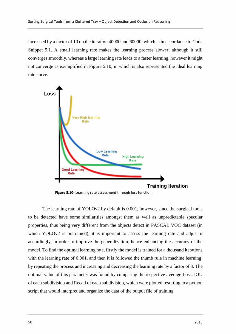
Sorting Surgical Tools from a Cluttered Tray – Object Detection and Occlusion Reasoning
50 2018
increased by a factor of 10 on the iteration 40000 and 60000, which is in accordance to Code
Snippet 5.1. A small learning rate makes the learning process slower, although it still
converges smoothly, whereas a large learning rate leads to a faster learning, however it might
not converge as exemplified in Figure 5.10, in which is also represented the ideal learning
rate curve.
The learning rate of YOLOv2 by default is 0.001, however, since the surgical tools
to be detected have some similarities amongst them as well as unpredictable specular
properties, thus being very different from the objects detect in PASCAL VOC dataset (in
which YOLOv2 is pretrained), it is important to assess the learning rate and adjust it
accordingly, in order to improve the generalization, hence enhancing the accuracy of the
model. To find the optimal learning rate, firstly the model is trained for a thousand iterations
with the learning rate of 0.001, and then it is followed the thumb rule in machine learning,
by repeating the process and increasing and decreasing the learning rate by a factor of 3. The
optimal value of this parameter was found by comparing the respective average Loss, IOU
of each subdivision and Recall of each subdivision, which were plotted resorting to a python
script that would interpret and organize the data of the output file of training.
Figure 5.10- Learning rate assessment through loss function.

Diana Martins Lavado 51
5.4.1.1. Learning Rate for Object Detection
In Figure 5.11(a) it is displayed the plots of average Loss, IOU of each subdivision
and Recall of each subdivision for a learning rate of 0.001 and from analyzing the loss graph
in comparison with Figure 5.10, it is possible to affirm that the learning rate is too high,
which was corroborated by Figure 5.11(b) in which the learning rate was increased to 0.003.
By reducing the learning rate to 0.0003, Figure 5.11(c), it is possible to observe an
improvement on Recall and slightly on IOU, however, the loss graph indicates that the
(a)
(b)
(c)
Figure 5.11- Plots of average Loss, IOU of each subdivision and Recall of each subdivision for object detection with learning rates of: (a) 0.001 (b) 0.003 (c) 0.0003.

Sorting Surgical Tools from a Cluttered Tray – Object Detection and Occlusion Reasoning
52 2018
learning rate is still high, which led to the training for learning rates of 0.0001, 0.00003 and
0.00001, which results are shown on Figure 5.12.
From the plots displayed on Figure 5.12 is possible to conclude that 0.0001 is the
most suitable learning rate, since it achieves lower values of loss than 0.00003 and 0.00001,
although the curve from Figure 5.12(b) is smother. Regarding the IOU and Recall, it is also
corroborated that 0.0001 (Figure 5.12(a)) is the best parameter, due to the best results
accomplished by 0.00003 (Figure 5.12(b)) and 0.00001 (Figure 5.12(c)) as learning rate.
(a)
(b)
(c)
Figure 5.12- Plots of average Loss, IOU of each subdivision and Recall of each subdivision for object detection with learning rates of: (a) 0.0001 (b) 0.00003 (c) 0.00001.

Diana Martins Lavado 53
5.4.1.1. Learning Rate for Occlusion Reasoning
With resemblance of the previous section, for occlusion reasoning it is also necessary
to find the optimal learning rate and the process is the same as previously described but
starting with the learning rate of 0.0001, which was the chosen value for object detection.
The first approach was to use the same test and train groups used in the training of the object
detection neural network, however, instead of resorting to the object detection labels, the
occlusion reasoning labels (with the classes top and bottom) were used.
The results from the first thousand iterations of the training with the learning rate of
0.0001 are displayed on Figure 5.13(a), and by observing the loss plot it can be considered
too large as well, as the learning rate from Figure 5.13(b). Amongst all the values tested for
the learning rate for occlusion reasoning, 0.00003 (Figure 5.13(c)) achieved the best results,
however, the loss curve should be smoother, indicating that the learning rate needs to be
decreased, which leads to bad recall results as shown in Figure 5.13(d).
Since none of the learning rates were suitable to perform occlusion detection, instead
of using one neural network, 4 different neural networks were trained, one per each
instrument class. Therefore, it was required to assess the best value of learning rate for each
class of surgical tool.
In Figure 5.14, Figure 5.15, Figure 5.16 and Figure 5.17 are presented the results
from the learning rates of 0.0001 (a), 0.0003 (b), 0.00003 (c), 0.00001 (d) applied to the
occlusion reasoning of scalpel, straight dissection clamp, straight mayo scissor and curved
mayo scissor, respectively. The optimal leaning rate for scalpel and straight dissection clamp
is 0.0001 because both Figure 5.14(a) and Figure 5.15(a) show the best results regarding the
loss curve, IOU and recall. Relatively to straight mayo scissor and curved mayo scissor,
according to Figure 5.16(c) and Figure 5.17(c), the learning rate of 0.00003 would be the
most appropriate, however since the tendency was to choose the learning rate 0.0001 another
thousand iterations were trained with both learning rates for both instruments and it was
verified that 0.0001 was indeed better.
There is an alternative method to find the optimal learning rate, which consists on
enabling “burn_in=1000” in the configuration file of the network that leads to a successive
increase of the learning rate up to the value chosen on the one thousand iteration, thus assess
the loss values and the corresponding learning rates.

Sorting Surgical Tools from a Cluttered Tray – Object Detection and Occlusion Reasoning
54 2018
(a)
(b)
(c)
Figure 5.13- Plots of average Loss, IOU of each subdivision and Recall of each subdivision for occlusion reasoning with learning rates of: (a) 0.0001 (b) 0.0003 (c) 0.00003 (d) 0.00001.
(d)

Diana Martins Lavado 55
(a)
(b)
(c)
Figure 5.14- Plots of average Loss, IOU of each subdivision and Recall of each subdivision for scalpel occlusion reasoning with learning rates of: (a) 0.0001 (b) 0.0003 (c) 0.00003 (d) 0.00001.
(d)

Sorting Surgical Tools from a Cluttered Tray – Object Detection and Occlusion Reasoning
56 2018
(a)
(b)
(c)
Figure 5.15- Plots of average Loss, IOU of each subdivision and Recall of each subdivision for straight dissection clamp occlusion reasoning with learning rates of: (a) 0.0001 (b) 0.0003 (c) 0.00003 (d) 0.00001.
(d)

Diana Martins Lavado 57
(a)
(b)
(c)
Figure 5.16- Plots of average Loss, IOU of each subdivision and Recall of each subdivision for straight mayo scissor occlusion reasoning with learning rates of: (a) 0.0001 (b) 0.0003 (c) 0.00003 (d) 0.00001.
(d)

Sorting Surgical Tools from a Cluttered Tray – Object Detection and Occlusion Reasoning
58 2018
(a)
(b)
(c)
Figure 5.17- Plots of average Loss, IOU of each subdivision and Recall of each subdivision for curved mayo scissor occlusion reasoning with learning rates of: (a) 0.0001 (b) 0.0003 (c) 0.00003 (d) 0.00001.
(d)

Diana Martins Lavado 59
5.5. Console Application
Before explaining the console application developed, it is necessary to understand
the overall methodology proposed in this dissertation, which is schematized in Figure 5.18.
The proposed method in this dissertation is to initially apply the YOLOv2 trained for
surgical tools detection, which returns the location of the detected tools in the image or video
frame as well as the object classification (scalpel, straight dissection clamp, straight mayo
scissor or curved mayo scissor). After obtaining the detection list, it is then sorted by
decrescent order, and the image is segmented at the location correspondent to the detection
with higher confidence score. Since the class of the chosen tool is known, then the respective
trained YOLOv2 for occlusion reasoning of that instrument is implemented and the object
is classified as being on top (not occluded), which determines the tool to be removed or, if
it is at the bottom (occluded), then the procedure is repeated for the next detection in the
sorted list until an instrument is classified as on top. The step following the determination of
the tool that is going to be extracted corresponds to pose estimation, in which the coordinates
obtained through YOLOv2 are converted to real world coordinates passible of being
understood by a robot, in order to sort the tools and to allow the assembly of specific surgical
kits.
Figure 5.18- Scheme of the proposed methodology to assemble surgical kits.

Sorting Surgical Tools from a Cluttered Tray – Object Detection and Occlusion Reasoning
60 2018
Since the target users of this system are nurses and hospital staff responsible for
sorting the surgical tools after being disinfected, it was necessary to develop an intuitive
application, otherwise it would be required skilled professionals to apply the neural networks
resorting to the PowerShell.
Initially, it was developed a Graphical User Interface in C++/CLI, however, due to
time limitations to finish this dissertation, a C++ console application was developed on
Microsoft Visual Studio (MVS) prompting the user to choose options within several menus.
Although the third version of YOLO was implemented in the final stages of this
dissertation, the main neural network architecture used was YOLOv2, which is included in
the dnn module of OpenCV library. However, instead of implementing the method resorting
to this library, which is very restrict regarding architectures and functionalities, it was
included the darknet dynamic link library (dll) into the project.
The first step towards the inclusion of darknet into the console application project is
to go to the directory “C:\darknet\build\darknet” and open and compile the project
“yolo_cpp_dll.vcxproj” that generates the necessary dll’s. This project is then added on MSV
to the console application project, thus requiring to be linked to the main project, which is
achieved by selecting the console application project and add a reference to “yolo_cpp_dll”.
Other essential additions are “yolo_v2_class.hpp” to the header files and “yolo_cpp_dll.dll”,
“pthreadGC2.dll” and “pthreadVC2.dll” to the project itself. Besides these steps its
necessary to check whether the solution configuration is release and the platform x64 as well
as the inclusion of all the required directories and libraries in the solution properties, which
are the following:
• Platform Toolset Visual Studio 2015(v140), as shown in Figure 5.19, because
the compiler of MVS 2017 is different and is not able to successfully compile the darknet;
• OpenCV include and library directories in VC++ Directories (Figure 5.20);
• “C:\opencv_3.0\opencv\build\include” as an additional include directory in
C/C++ >General;
• Additional library directories shown in Figure 5.21;
• Additional dependencies shown in Figure 5.22.

Diana Martins Lavado 61
Figure 5.19- Platform Toolset property.
Figure 5.20- OpenCV include and library directories.

Sorting Surgical Tools from a Cluttered Tray – Object Detection and Occlusion Reasoning
62 2018
Figure 5.22- OpenCV additional dependencies.
Figure 5.21- OpenCV and pthreads additional library directories.

Diana Martins Lavado 63
After the setup of the MVS environment it was built a function for each menu
presented in Figure 5.23.
Whenever the application is launched the menu displayed in Figure 5.23(a) is shown.
If users choose the option 1 then Figure 5.23(b) is displayed, whereas if options 2, 3 or 4 are
chosen the menu from Figure 5.23 (c) appears.
The first menu lists all the currently loaded files. For that, it was created a struct
named network_data with name, configuration and weight file names as attributes and 5
instances of the struct (one for object detection and four for occlusion reasoning of each
instrument) were defined with the respective attributes. After the user choose one of the first
5 options of the menu Figure 5.23(c) and insert the name of the new file, the attribute
correspondent of the previous selected option on Figure 5.23(a) menu in the respective
instance indicated by the selected option on Figure 5.23 (c) will be modified.
Both the option Change files in Figure 5.23(b) and Return in Figure 5.23(c) lead to
the Figure 5.23(a) menu and the current menu remains until a valid option is inserted.
The main menu, Figure 5.23(b), has two principal options:
• Detect objects, which supports both video and images returning the
classification of every object detected in the image as well the respective confidence score;
(a)
(b)
(c)
Figure 5.23- Console application menus (a) Files loaded (b) Main menu (c) Change files menu.
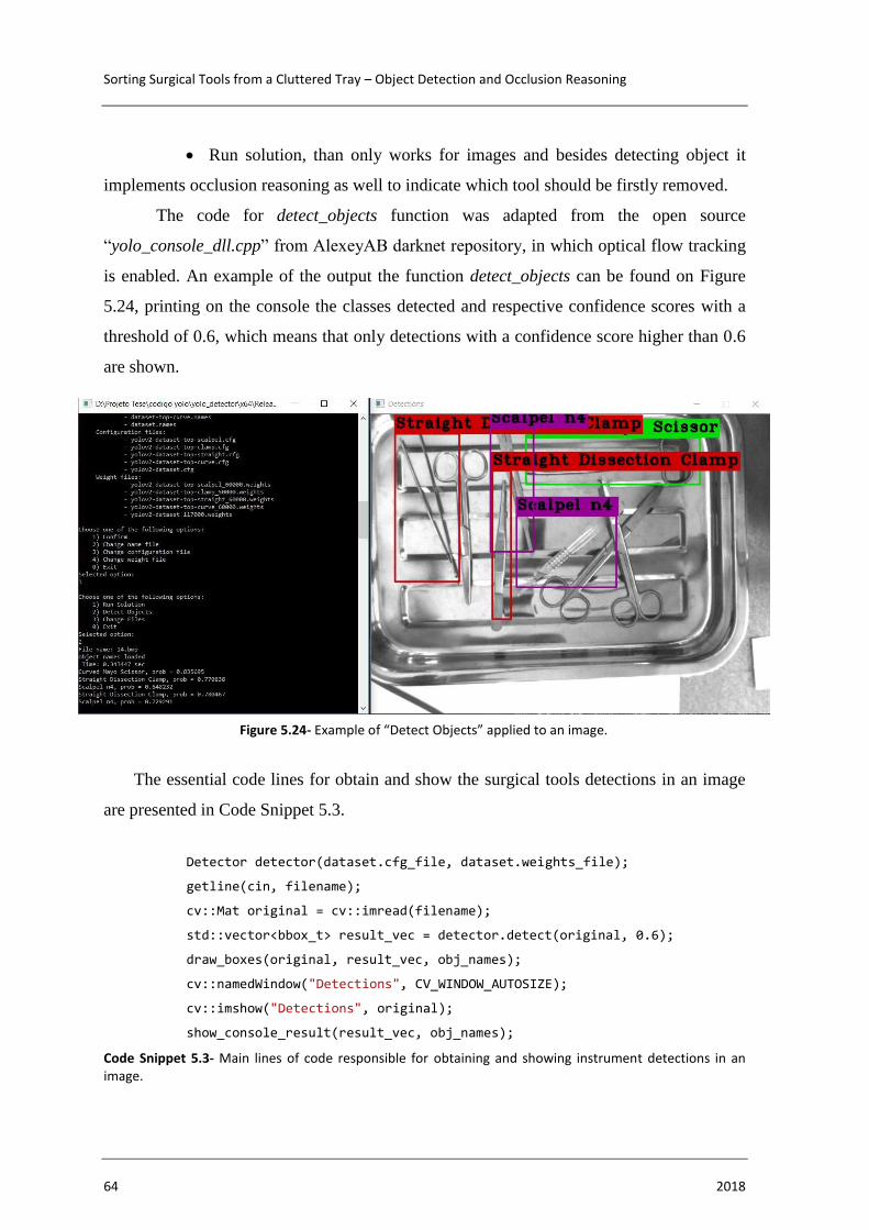
Sorting Surgical Tools from a Cluttered Tray – Object Detection and Occlusion Reasoning
64 2018
• Run solution, than only works for images and besides detecting object it
implements occlusion reasoning as well to indicate which tool should be firstly removed.
The code for detect_objects function was adapted from the open source
“yolo_console_dll.cpp” from AlexeyAB darknet repository, in which optical flow tracking
is enabled. An example of the output the function detect_objects can be found on Figure
5.24, printing on the console the classes detected and respective confidence scores with a
threshold of 0.6, which means that only detections with a confidence score higher than 0.6
are shown.
The essential code lines for obtain and show the surgical tools detections in an image
are presented in Code Snippet 5.3.
Detector detector(dataset.cfg_file, dataset.weights_file);
getline(cin, filename);
cv::Mat original = cv::imread(filename);
std::vector<bbox_t> result_vec = detector.detect(original, 0.6);
draw_boxes(original, result_vec, obj_names);
cv::namedWindow("Detections", CV_WINDOW_AUTOSIZE);
cv::imshow("Detections", original);
show_console_result(result_vec, obj_names);
Code Snippet 5.3- Main lines of code responsible for obtaining and showing instrument detections in an image.
Figure 5.24- Example of “Detect Objects” applied to an image.

Diana Martins Lavado 65
In order to fully understand the Code Snippet 5.3, it is important to clarify the following:
• “Detector” is a class defined on the header file “yolo_v2_class.hpp”;
• “dataset” is an instance of a network_data struct previously mentioned and
cfg_file and weights_file are respective attributes;
• “bbox_t” is a struct with information regarding a detection such as x and y
coordinates of the top left corner of the bounding box, as well as width,
height, confidence score, class id, track id and frame counter;
• “result_vec” is a vector in which the bbox_t of all detections with confidence
scores higher than 0.6 are stored;
• “draw_boxes”, as the name indicates, is a function that overlaps the bounding
boxes and respective labels with the original image;
• “show_console_result” is the function for displaying the detections class and
confidence scores onto the console.
Regarding the solution_img function, the first step is to detect the instruments present
in the image resorting to the code lines shown in Code Snippet 5.3. Afterwards, it is applied
a function to sort the detections with decrescent order of confidence score and the result list
of detections has the name sorted_vec. In accordance with the scheme of Figure 5.18, the
next step is to choose the first two detections of sorted_vec (with higher confidence score)
and for each segment the original image is segmented at the bounding box coordinates and
it was applied the respective occlusion reasoning network, as shown in Code Snippet 5.4.
Due to memory limitations there could only be one occlusion reasoning detector, alternating
between the neural networks correspondent to each class as need.
for (int i = 0; i < max_num; i++) { Detector occlusion_detector(list_net_data[sorted_vec[i].obj_id].cfg_file, list_net_data[sorted_vec[i].obj_id].weights_file); //Segment original image at sorted_vec[i] coordinates Rect ROI(sorted_vec[i].x, sorted_vec[i].y, sorted_vec[i].w, sorted_vec[i].h); Mat mask(original.size(), CV_8UC1, Scalar::all(0)); mask(ROI).setTo(Scalar::all(255)); original.copyTo(cropped_img, mask); //execute the respective occlusion detector and store the results std::vector<bbox_t> result_vec2 = occlusion_detector.detect(cropped_img, 0.6); std::vector<bbox_t> sorted_vec2 = sort_vector(result_vec2); result_occlusion.push_back(sorted_vec2[0]); }
Code Snippet 5.4- Part of the algorithm for occlusion reasoning

Sorting Surgical Tools from a Cluttered Tray – Object Detection and Occlusion Reasoning
66 2018
The max_num is set to 2 because it is intended have two options (if possible) of tools
to be removed from the tray at the end of the algorithm and implement a voting system in
order to choose the best one, however this value can be changed by the user, thus the
algorithm implements foolproof conditions, e.g. the max_num need to be lower than the
number of detections on the image, otherwise max_num takes the value of total number of
detections. It is important to mention that the higher the value of max_num, the greater is the
computational power required and, consequently, the higher the running time of the
algorithm.
For the first max_num (in this dissertation has the value 2) detections of the sorted
list, the occlusion detector respective to the instrument class of the detection is initialized,
the image is segmented in order to remove the background, easing the detecting and
improving the accuracy of the classification as top (not occluded) of bottom (occluded). If
the tool is classified as bottom, then it is discarded as a valid option and in the end, all the
top valid detections can be assessed through the multiplication between the object detection
confidence score and occlusion reasoning confidence score. Therefore, the instrument
detection with the highest value resultant from this multiplication corresponds to the surgical
tool to be removed by the robot.

Diana Martins Lavado 67
6. RESULTS
6.1. Classical Approach Results
As previous discussed in Section 4.1.3, the following figures present the final
watershed models and contours for each tool.
(a) (b)
Figure 6.1- Scalpel nº4 (a) contours (b) watershed model.
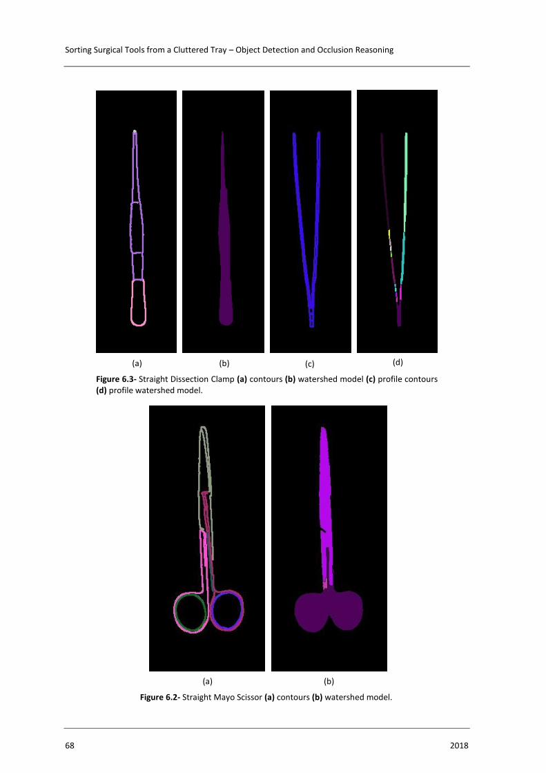
Sorting Surgical Tools from a Cluttered Tray – Object Detection and Occlusion Reasoning
68 2018
(a) (b) (c) (d)
Figure 6.3- Straight Dissection Clamp (a) contours (b) watershed model (c) profile contours (d) profile watershed model.
(a) (b)
Figure 6.2- Straight Mayo Scissor (a) contours (b) watershed model.

Diana Martins Lavado 69
6.2. Modern Approach Results
6.2.1. Object Detection Results
After the training of the neural networks it is necessary to choose the iteration of
which weights are responsible for achieving the best results and the first step is to plot the
precision-recall curve.
The precision-recall curve is a good method for assessing the classifier
performance by analyzing the precision and recall evolution as the threshold change,
however besides requiring high computational power and memory, the process to compute
the values for each weigh iteration is too time consuming. Therefore, it was only generated
the data to plot the curve with weights respective 100 000, 150 000 and 200 000 iterations.
(a) (b)
Figure 6.4- Curved Mayo Scissor (a) contours (b) watershed model.

Sorting Surgical Tools from a Cluttered Tray – Object Detection and Occlusion Reasoning
70 2018
In order to understand the meaning of precision and recall it is necessary to
introduce the concept of a confusion matrix which is represented on Table 6.1.
Table 6.1- Symbolic confusion matrix.
Prediction Class
Positive Negative
Act
ual
Cla
ss
Positive True Positive
(TP)
False Positive
(FP)
Negative False Negative
(FN)
True Negative
(TN)
The precision represents the percentage of correct detections of a class and are
actually correct and its expression is given by Equation 6.1, whereas the recall indicated the
proportion of a determined class that was identified correctly through Equation 6.2.
𝑝𝑟𝑒𝑐𝑖𝑠𝑖𝑜𝑛 =𝑇𝑃
𝑇𝑃+𝐹𝑃 (6.1)
𝑟𝑒𝑐𝑎𝑙𝑙 = 𝑇𝑃
𝑇𝑃+𝐹𝑁 (6.2)
Neither the pjreddie or the AlexeyAB repositories for darknet have a function to
obtain the necessary data, hence, it was added on detector.c the code presented in Annex B
to allow the plot of precision-recall curves by a matlab script.
The acquisition of the precision and recall for each value of threshold (varying
from 0 to 1 in intervals of 0.01) can be achieved by typing “./darknet detector PRcurve path-
to-data path-to-cfg path-to-weight” onto the Ubuntu terminal.
The precision-recall curve of weights respective to the iterations 100000, 150000
and 200000 is shown in Figure 6.5, in which we can observe that the best results are achieved
by the weights of 100000 iteration, which indicate that by the iteration number 200000 the
neural network may be overfitted, due to “memorization” of images losing its generalization
ability. From the same graph, the extremity point of each curve is chosen, and its
correspondent threshold value is found and used in the following analysis step.

Diana Martins Lavado 71
Therefore, threshold values for 100000, 150000 and 200000 iterations are
respectively 0.35, 0.45 and 0.45.
The next step is to find the iteration number which achieves the best mAP and IOU
results on the test group, because training the network too much leads to a memorization of
images and a decreased ability of generalization and, on the other hand, not training enough
results in a method, which performance could be improved. In order to acquire the necessary
data, it is used the AlexeyAB fork of darknet, because it has a function that returns the
required values in a text file per weight, which are then organized and analyzed by a
developed matlab function. This data could be achieved through typing “./darknet detector
map path-to-data path-to-cfg path-to-weighs -thresh threshold_value” on the ubuntu
terminal however, since it was necessary to follow this procedure for several weight files, it
Figure 6.5- Precision-recall curve of weights respective to 100 000, 150 000 and 200 000 iterations.

Sorting Surgical Tools from a Cluttered Tray – Object Detection and Occlusion Reasoning
72 2018
was developed a python script that has the minimum, maximum and interval of weights as
an input, and automatically executes the respective command on the terminal with thresholds
according to the ones found through the precision-recall curve.
Firstly, to assess the round value of the ideal iteration number, it was executed the
python script previously described for every five thousand iterations between 75 000 and
200 000 iterations, in which if the current iteration number was equal or higher than 150 000,
the threshold value was 0.45, whereas if it was inferior, then the threshold was 0.35. After
the generation of the data, the text files were converted to winfiles and loaded to matlab,
which enabled a better data visualization easing the iteration choice through the analysis of
Figure 6.6.
The best iteration number is the one presenting higher mAP and IOU values, which
corresponds to the point closer to the top right corner of Figure 6.6.
From the analysis of this graph, it is possible to conclude that the choice of the best
iteration number is between two points, assigned respectively to 100000 (blue) and 185000
(yellow) iterations. The difference of both mAP values corresponds to 0.01%, whereas the
Figure 6.6- Plot of IOU in function of mAP for every five thousand iterations between 55000 and 200000 iterations.

Diana Martins Lavado 73
difference of the IOU parameters is 0.17%, thus they are approximately at the same distance
of the top right corner. Therefore, the optimal iteration number is located near 100 000
iterations, because in bin-picking applications it is preferable to have an improved
localization detection of the tools at the cost of 0.01% in the mAP value.
In order to find the exact optimal iteration number, the process was repeated for every
thousand iterations between 75 000 and 125 000 iterations, and the results are shown in
Figure 6.7.
Once again, the decision of the exact optimal iteration number lies in the choice
between two points, respective to 100000 (green) and 117000 (yellow) iterations, in which
the mAP difference is 0.02% and the IOU difference is 0.12% however, instead of following
the logic previously described, it is chosen the closest point to the corner which is the yellow,
meaning that YOLOv2 achieves the best performance detecting surgical tools with the
weights of 117 000 iterations, accomplishing a IOU of 72.62% and a mAP of 90.06%, which
is discriminated per each class in Table 6.2.
Figure 6.7- Plot of IOU in function of mAP for every thousand iterations between 75000 and 125000 iterations.

Sorting Surgical Tools from a Cluttered Tray – Object Detection and Occlusion Reasoning
74 2018
Table 6.2- Discrimination of average precision per class corresponding to 117000 iterations during training.
From the observation of Table 6.2, it is possible to verify that the scalpel has the
highest average precision amongst the tested surgical tools, which is due to being the most
different from the other instruments.
Another measure usually used to assess the model performance is F1 score, which
balances precision and recall and its formula can be found on Equation 6.3 applied to 117000
iterations.
𝐹1 = 2 ×𝑃𝑟𝑒𝑐𝑖𝑠𝑖𝑜𝑛×𝑅𝑒𝑐𝑎𝑙𝑙
𝑃𝑟𝑒𝑐𝑖𝑠𝑖𝑜𝑛+𝑅𝑒𝑐𝑎𝑙𝑙× 100 = 2 ×
0.88×0.95
0.88+0.95 × 100 = 91.4% (6.3)
Finally, in order to classify the type of error of the neural network it was used the
methodology of Hoiem [149]. However, to apply that method it was necessary the IOU,
predicted class and actual class of each detection on the test group. To acquire that data, the
map function (named validate_detector_map) from the AlexeyAB darknet repository was
modified with the addition of the code “printf(“ IOU = %f, prob = %f, class_id = %d,
truth_id = %d \n”, box_iou(dets[i].bbox, t), prob, class_id, truth[j].id);” and afterwards the
framework was recompiled.
The data was analyzed resorting to matlab, in which the detections were classified
with the following categories:
• Correct: correct class and IOU≥0.5;
• Localization: correct class and 0.1<IOU<0.5;
• Similar: class is similar (both scissors) and IOU>0.1;
• Other: class is wrong and IOU>0.1;
• Background: IOU<0.1.
Surgical Tool Average Precision (%)
Scalpel nº4 90,66
Straight Dissection Clamp 89,42
Straight Mayo Scissor 90,40
Curved Mayo Scissor 89,75

Diana Martins Lavado 75
The Figure 6.8 displays a pie chart with the percentages of each error for detections
with a confidence score higher than 60% (threshold) in a total of 1721 detections, using the
weights after 117000 iterations of training.
6.2.1.1. Cross Validation
The importance of cross validation and respective split of the dataset into train and
test groups is described in Section 5.3.1, and the results analysis is the same as detailed in
the previous section.
The precision-recall curve for cross-validation weight correspondent to 100 000, 150
000 and 200 000 iterations is displayed in Figure 6.9, and it can be verified that it is in
accordance with Figure 6.5.
Resembling the previous section, the best iteration number for training during cross-
validation is found through Figure 6.10, which shows lower mAP and IOU values in
comparison with Figure 6.7, however, still evidencing the good performance of the neural
network. From the analysis of the graph, the ideal iteration number is 140 000 iterations,
which is the closest point to the top right corner, presenting a mAP of 89.13% and a IOU of
67.28%.
57%
1%
5%
17%
20%
Error Analysis YOLOv2
Correct
Localization
Similar
Other
Background
Figure 6.8- Pie chart with the discrimination of YOLOv2 errors for object detection.

Sorting Surgical Tools from a Cluttered Tray – Object Detection and Occlusion Reasoning
76 2018
Figure 6.9- Precision-recall curve of cross-validation weights respective to 100 000, 150 000 and 200 000 iterations.
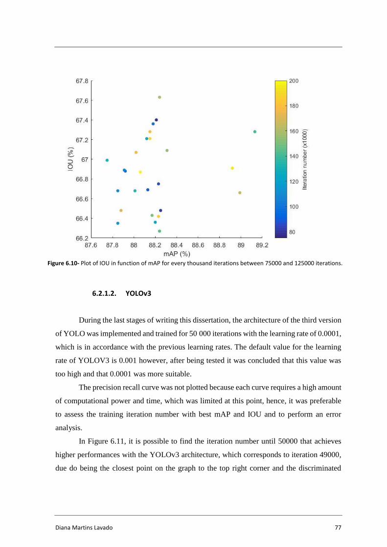
Diana Martins Lavado 77
6.2.1.2. YOLOv3
During the last stages of writing this dissertation, the architecture of the third version
of YOLO was implemented and trained for 50 000 iterations with the learning rate of 0.0001,
which is in accordance with the previous learning rates. The default value for the learning
rate of YOLOV3 is 0.001 however, after being tested it was concluded that this value was
too high and that 0.0001 was more suitable.
The precision recall curve was not plotted because each curve requires a high amount
of computational power and time, which was limited at this point, hence, it was preferable
to assess the training iteration number with best mAP and IOU and to perform an error
analysis.
In Figure 6.11, it is possible to find the iteration number until 50000 that achieves
higher performances with the YOLOv3 architecture, which corresponds to iteration 49000,
due do being the closest point on the graph to the top right corner and the discriminated
Figure 6.10- Plot of IOU in function of mAP for every thousand iterations between 75000 and 125000 iterations.

Sorting Surgical Tools from a Cluttered Tray – Object Detection and Occlusion Reasoning
78 2018
results can be consulted on Table 6.3, allowing to confirm the higher performance of
YOLOv3 in comparison with the previous version.
Table 6.3- YOLOv3 results discrimination for resultant weights of 49000 iteration of training.
The Figure 6.12 displays a pie chart with the percentages of each error for detections
with a confidence score higher than 60% (threshold) in a total of 1869 detections, using the
weights after 49000 iterations of training. The main difference between this YOLO version
and the previous is the percentage of correct detections is approximately 1% lower for
YOLOv3, however, it is important to mention that this method identifies almost more 150
detections the YOLOv2, thus the confident scores of each detection are much higher for the
most recent version.
mAP IOU F1 Scalpel AP Straight Dissect.
Clamp AP
Straight Mayo
Scissor AP
Curved Mayo
Scissor AP
91,98% 78,93% 94% 90,03 % 90,72 % 90,47 % 96,68 %
Figure 6.11- Plot of IOU in function of mAP for every thousand iterations between 1000 and 50000 iterations for YOLOv3.

Diana Martins Lavado 79
6.2.2. Occlusion Reasoning
With regard to the 4 occlusion reasoning neural networks, the respective data is
severely imbalanced, due to the existence of a significant higher quantity of examples in
which each tool is on top of the pile (or does not present occlusion) rather than on the bottom
(being occluded).
The precision-recall curve is usually not significantly affected by imbalanced data,
however, this graph is not applicable to the data generated through darknet due to the uneven
split of data per each class (top or bottom).
The neural networks aiming to overcome the occlusion challenge were trained for
50 000 or 60 000 iterations, due to time limitations of this dissertation, therefore, the optimal
iteration number was not found and the weights resultant from training that achieved the best
performance are respective to the last iteration number, which can be verified by analyzing
Figure 6.13, Figure 6.14, Figure 6.15, Figure 6.16, in which the last point is closer to the top
right corner in every graph. The respective mAP and IOU can be found in Table 6.4.
56%
1%
5%
19%
19%
Error Analysis YOLOv3
Correct
Localization
Similar
Other
Background
Figure 6.12- Pie chart with the discrimination of YOLOv3 errors for object detection.

Sorting Surgical Tools from a Cluttered Tray – Object Detection and Occlusion Reasoning
80 2018
Figure 6.14- Plot of IOU in function of mAP for every thousand iterations between 10000 and 50000 iterations for straight dissection clamp occlusion reasoning.
Figure 6.13- Plot of IOU in function of mAP for every thousand iterations between 10000 and 60000 iterations for scalpel occlusion reasoning.
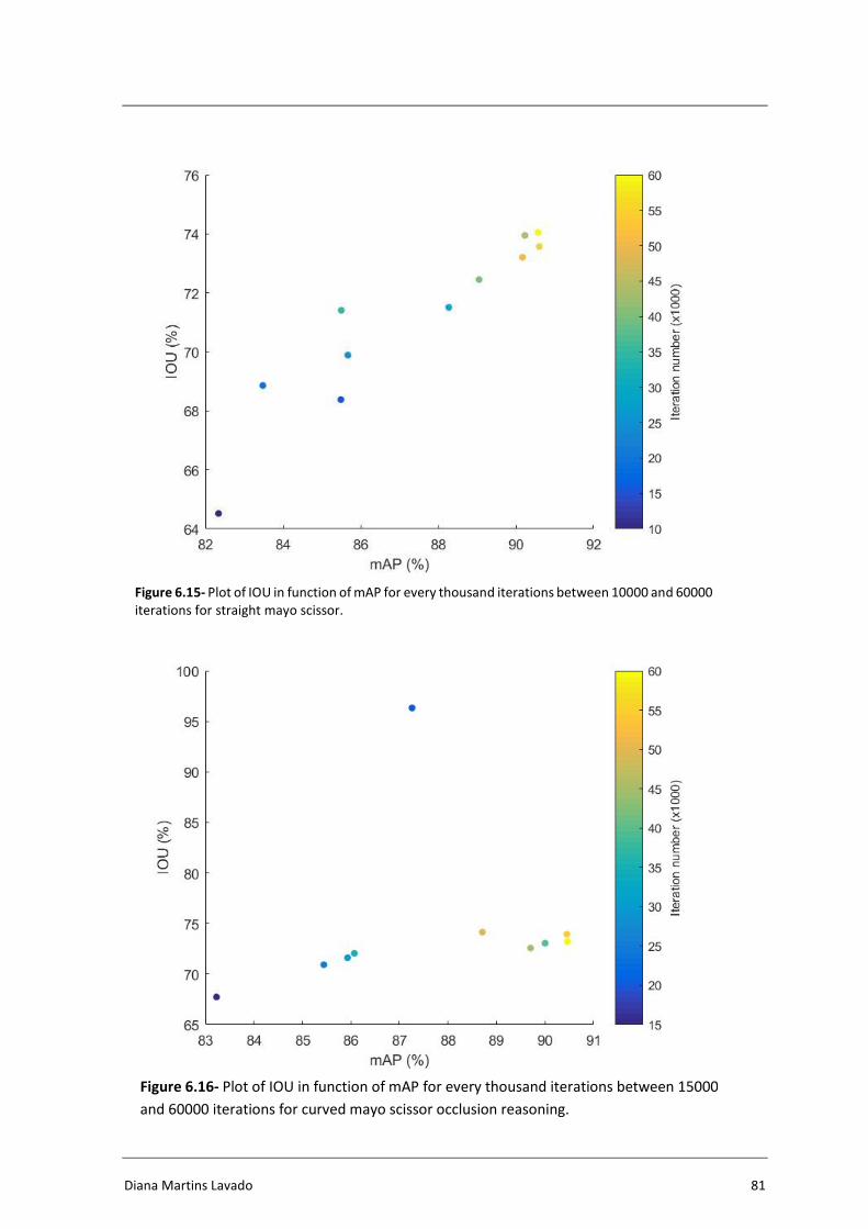
Diana Martins Lavado 81
Figure 6.16- Plot of IOU in function of mAP for every thousand iterations between 15000
and 60000 iterations for curved mayo scissor occlusion reasoning.
Figure 6.15- Plot of IOU in function of mAP for every thousand iterations between 10000 and 60000 iterations for straight mayo scissor.

Sorting Surgical Tools from a Cluttered Tray – Object Detection and Occlusion Reasoning
82 2018
Table 6.4- mAP and IOU relative to the weights of the last trained iteration for the occlusion reasoning network of each instrument.
The results of error analysis for the occlusion reasoning neural networks, resembling
the one described in Section 6.2.1, can be found in Table 6.5. In this table there is not a
“similar” category, because the two classes (top and bottom) that these networks distinguish
are very different, and the occlusion reasoning performance of the scalpel neural network is
higher, because this surgical tool is the most unalike with the other instruments. Through the
same reasoning, it is possible to justify the slightly lower performance of both types of
scissor, due to their similarities.
Table 6.5- Error analysis for each occlusion reasoning neural network respective to each surgical tool.
Scalpel
Straight
Dissection
Clamp
Straight Mayo
Scissor
Curved Mayo
Scissor
#detection>55% 315 318 293 356
Correct 95,23 % 93,71 % 92,49 % 88,76 %
Location 0,00 % 0,31 % 1,71 % 1,69 %
Other 4,44 % 5,03 % 3,07 % 4,49 %
Background 0,32 % 0,94 % 2,73 % 5,06 %
Surgical Tool Mean Average Precision (%) IOU(%)
Scalpel nº4 89,09 79,35
Straight Dissection Clamp 91,82 74,59
Straight Mayo Scissor 90,57 74,05
Curved Mayo Scissor 90,46 73,21
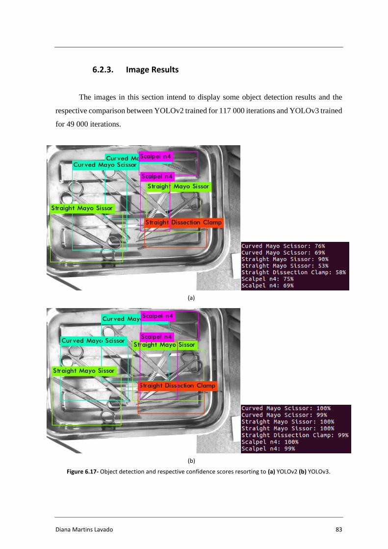
Diana Martins Lavado 83
6.2.3. Image Results
The images in this section intend to display some object detection results and the
respective comparison between YOLOv2 trained for 117 000 iterations and YOLOv3 trained
for 49 000 iterations.
(a)
(b)
Figure 6.17- Object detection and respective confidence scores resorting to (a) YOLOv2 (b) YOLOv3.

Sorting Surgical Tools from a Cluttered Tray – Object Detection and Occlusion Reasoning
84 2018
Figure 6.17 and Figure 6.18 allow to observe that YOLOv3 detects more objects in
the image and performs better localization, as well as it always presents a much higher
confidence score in comparison with YOLOv2.
(a)
(b)
Figure 6.18- Object detection and respective confidence scores resorting to (a) YOLOv2 (b) YOLOv3.

Diana Martins Lavado 85
Both versions of YOLO are robust to clutter, as shown in Figure 6.19 and Figure
6.20 and, once again YOLOv3 demonstrated its performance superiority. In Figure 6.20, it
is possible to verify a detection error by YOLOv2, which mistook a straight mayo scissor
for a curved mayo scissor.
(a)
(b)
Figure 6.19- Object detection and respective confidence scores resorting to (a) YOLOv2 (b) YOLOv3.
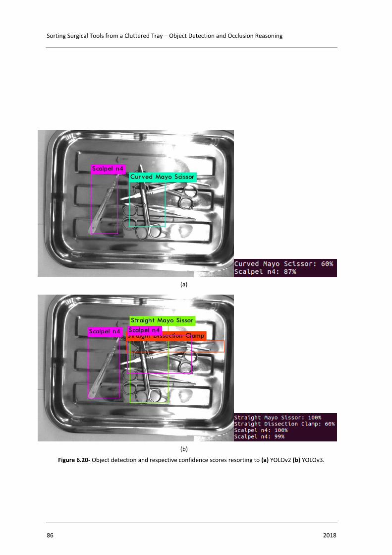
Sorting Surgical Tools from a Cluttered Tray – Object Detection and Occlusion Reasoning
86 2018
(a)
(b)
Figure 6.20- Object detection and respective confidence scores resorting to (a) YOLOv2 (b) YOLOv3.

Diana Martins Lavado 87
Figure 6.21 and Figure 6.22 show the performance of the two latest version of YOLO
in poor lit conditions.
(a)
(b)
Figure 6.21- Object detection and respective confidence scores resorting to (a) YOLOv2 (b) YOLOv3.

Sorting Surgical Tools from a Cluttered Tray – Object Detection and Occlusion Reasoning
88 2018
(a)
(b)
Figure 6.22- Object detection and respective confidence scores resorting to (a) YOLOv2 (b) YOLOv3.

Diana Martins Lavado 89
Figure 6.23 intends to prove that these methods can be implemented on surgical
tools with a different background from the training images and still achieve great results.
(a)
(b)
Figure 6.23- Object detection and respective confidence scores resorting to (a) YOLOv2 (b) YOLOv3.
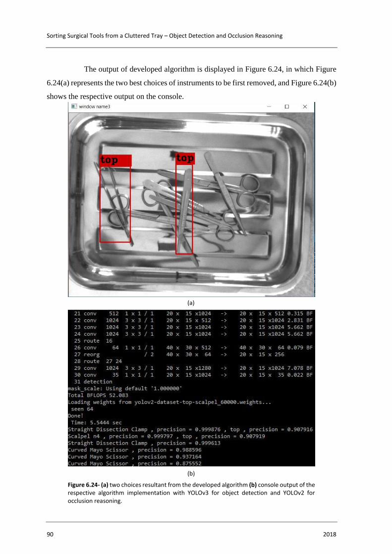
Sorting Surgical Tools from a Cluttered Tray – Object Detection and Occlusion Reasoning
90 2018
The output of developed algorithm is displayed in Figure 6.24, in which Figure
6.24(a) represents the two best choices of instruments to be first removed, and Figure 6.24(b)
shows the respective output on the console.
(a)
(b)
Figure 6.24- (a) two choices resultant from the developed algorithm (b) console output of the respective algorithm implementation with YOLOv3 for object detection and YOLOv2 for occlusion reasoning.

Diana Martins Lavado 91
7. FUTURE WORK
The overall challenges addressed in this dissertation can be divided into several
stages such as detection, occlusion reasoning, grasping point detection, pose estimation and
kit assembly. However, in this research the focus was on the first stage and trying to prove
that the occlusion reasoning was possible using neural networks.
Regarding object detection, the network architecture YOLOv3 achieved promising
results surpassing YOLOv2 and can be further improved by continuing the training of the
neural network, because according to Figure 6.11, the networks does not show signs of
overtraining (decrease in the IOU-map relation). Another way of increasing the performance
of the system is to approximate the grabbed instrument to the camera for validation of the
object classification or to attach the camera to the robot and move it closer to the instrument,
however the first approach should achieve better results due to distance between the surgical
tool removed and the background clutter.
The performance of occlusion reasoning using neural networks, with resemblance of
the object detection with YOLOv3, could be improved by training the respective neural
networks more time since none achieved the overtraining stage. When testing the several
learning rates for the occlusion reasoning network trained with images of all four classes of
surgical tools, the loss graph correspondent to the learning rate of 0.00003 (Figure 5.13(c))
looks promising despite the reasonable recall, therefore it would be interesting to train for
further iterations to better assess if it successfully detects whether a tool is on top or at the
bottom.
A possible future work for both object detection and occlusion reasoning is to test
other network architectures such as Faster R-CNN, which in the literature has a higher mean
average precision at the cost of increased running and training speed and YOLOv3 (for
occlusion reasoning).
The stage of grasping point detection was not developed, however, it is suggested to
label all the images for each class with the bounding box around the ideal grasping point and
to train the neural networks. For grasping point refinement, it could be used a pixel-voting

Sorting Surgical Tools from a Cluttered Tray – Object Detection and Occlusion Reasoning
92 2018
system similar to hough voting to determine the orientation of the tool and consequently, of
the robotic arm.
As for the type of gripper, one of the most used in bin-picking is a vacuum-gripper,
but it is not suitable for surgical tools because it requires planar surfaces and the exact
orientation of the tool. The second most popular gripper for this type of applications is a
magnetic gripper, however, different instruments have different weighs, and if the magnetic
force is too big, then it will grab more than a tool. Hence, it is proposed the use of an
electromagnetic gripper whose magnetic force is controlled through the definition of a
current, according to the instrument detected class.
The console application of this dissertation is still in its early stages of development,
which justifies shortcomings such as the code instability and inefficient memory allocation,
that can be the focus of further development. Thus, an important future work suggested is
the creation of an intuitive graphical user interface, as well as some addition of some
conditions to the algorithm for example to lower the detector threshold value if no surgical
tool is detected in the image or video frame.
Another essential part of the system that needs to be developed is the enabling of a
real time connection with the camera and implementation of the algorithm. Currently, in this
dissertation, the algorithm does not run is real-time, because it takes between 5 and 10
seconds to determine which tool should be removed, however, those values do not negatively
impact the system due to being lower than the necessary time for the robot to grab the
selected surgical tool and place it the appropriate place. Nevertheless, the algorithm run-time
can be significantly improved by acquiring better hardware, such as graphics cards with
more dedicated memory, because it would allow the continuous parallel running of different
detectors, as well as leading to an increased running speed.
All the neural networks were trained with the built dataset, however their
performance could be further improved by enlarging the dataset and apply data augmentation
techniques, despite YOLO already perform data augmentation during the training.

Diana Martins Lavado 93
8. CONCLUSIONS
This dissertation proposes a methodology based on deep learning neural networks to
identify the surgical tools present in a cluttered tray and execute occlusion reasoning for the
two detections with higher confidence score, thus indicating the instrument to be removed.
In the presented work, it is possible to conclude that the main objectives were
successfully achieved, accomplishing the following results:
• a mean average precision of 91,98% and IOU of 78,93% for object
classification through YOLOv3 after 49000 iteration of training;
• a mean average precision of 89,09% and IOU of 79,35% for scalpel occlusion
reasoning through YOLOv2 after 60000 iteration of training;
• a mean average precision of 91,82% and IOU of 74,59% for straight
dissection clamp occlusion reasoning through YOLOv2 after 50000 iteration
of training;
• a mean average precision of 90,57% and IOU of 74,05% for scalpel occlusion
reasoning through YOLOv2 after 60000 iteration of training;
• a mean average precision of 90,46% and IOU of 73,21% for scalpel occlusion
reasoning through YOLOv2 after 60000 iteration of training;
• the running of each detector of the neural networks above mentioned takes
around 0.2 seconds for an image or video frame, which allows real-time
monitoring;
• the running of the overall algorithm to select the tool to be removed takes
around 10 seconds, with the hardware mentioned on Table 3.1.
Although the results already are promising, there is still room for improvement,
which can be performed by implantation of the suggestions in Section 7.

Sorting Surgical Tools from a Cluttered Tray – Object Detection and Occlusion Reasoning
94 2018
Diana Martins Lavado 95
BIBLIOGRAPHY
[1] P. I. Buerhaus, D. I. Auerbach, and D. O. Staiger, “The recent surge in nurse
employment: Causes and implications,” Health Aff., vol. 28, no. 4, pp. 657–668, 2009.
[2] S. Schenkel, “Nurse staffing and inpatient hospital mortality.,” N. Engl. J. Med., vol.
364, no. 25, p. 2468; author reply 2469, 2011.
[3] H. Tan et al., “An integrated vision-based robotic manipulation system for sorting
surgical tools,” in IEEE Conference on Technologies for Practical Robot
Applications, TePRA, 2015, vol. 2015–Augus, pp. 1–6.
[4] T. Zhou and J. P. Wachs, “Needle in a haystack: Interactive surgical instrument
recognition through perception and manipulation,” Rob. Auton. Syst., vol. 97, pp.
182–192, 2017.
[5] G. S. Guthart and J. K. Salisbury, “The Intuitive telesurgery system: overview and
application,” Proc. 2000 ICRA. Millenn. Conf. IEEE Int. Conf. Robot. Autom. Symp.
Proc. (Cat. No.00CH37065), vol. 1, no. April, pp. 618–621, 2000.
[6] D. H. Boehm et al., “Clinical Use of a Computer-enhanced Surgical Robotic System
for Endoscopic Coronary Artery Bypass Grafting on the Beating Heart,” Thorac
Cardiovasc Surg, vol. 48, no. 04, pp. 198–202, 2000.
[7] M. G. Jacob, Y.-T. Li, and J. P. Wachs, “Gestonurse,” in Proceedings of the seventh
annual ACM/IEEE international conference on Human-Robot Interaction - HRI ’12,
2012.
[8] E. Carpintero, C. Pérez, R. Morales, N. García, A. Candela, and J. M. Azorín,
“Development of a robotic scrub nurse for the operating theatre,” in 2010 3rd IEEE
RAS and EMBS International Conference on Biomedical Robotics and
Biomechatronics, BioRob 2010, 2010.
[9] M. G. Jacob, Y. T. Li, and J. P. Wachs, “Surgical instrument handling and retrieval
in the operating room with a multimodal robotic assistant,” in Proceedings - IEEE
International Conference on Robotics and Automation, 2013.
[10] F. Miyawaki et al., “Development of automatic acquisition system of surgical-
instrument informantion in endoscopic and laparoscopic surgey,” in 2009 4th IEEE
Conference on Industrial Electronics and Applications, ICIEA 2009, 2009, pp. 3058–

Sorting Surgical Tools from a Cluttered Tray – Object Detection and Occlusion Reasoning
96 2018
3063.
[11] I. Sobel and G. Feldman, “A 3 × 3 Isotropic Gradient Operator for Image Processing,”
Stanford Artif. Intell. Proj., pp. 271–272, 1968.
[12] J. Canny, “A Computational Approach to Edge Detection,” IEEE Trans. Pattern Anal.
Mach. Intell., vol. PAMI-8, no. 6, pp. 679–698, 1986.
[13] C. Harris and M. Stephens, “A Combined Corner and Edge Detector,” Procedings
Alvey Vis. Conf. 1988, p. 23.1-23.6, 1988.
[14] E. Rosten and T. Drummond, “Machine Learning for High Speed Corner Detection,”
Comput. Vis. -- ECCV 2006, pp. 430–443, 2004.
[15] M. S. Extremal, J. Matas, O. Chum, M. Urban, and T. Pajdla, “Robust Wide Baseline
Stereo from,” Br. Mach. Vis. Conf., pp. 384–393, 2002.
[16] M. Basu and S. Member, “Gaussian-Based Edge-Detection Methods — A Survey,”
vol. 32, no. 3, pp. 252–260, 2002.
[17] W. Beck, J. O. Bockris, J. McBreen, and L. Nanis, “Hydrogen Permeation in Metals
as a Function of Stress, Temperature and Dissolved Hydrogen Concentration,” Proc.
R. Soc. A Math. Phys. Eng. Sci., vol. 290, no. 1421, pp. 220–235, 1966.
[18] D. G. Lowe, “Object recognition from local scale-invariant features,” Proc. Seventh
IEEE Int. Conf. Comput. Vis., pp. 1150–1157 vol.2, 1999.
[19] D. G. Lowe, “Distinctive image features from scale-invariant keypoints,” Int. J.
Comput. Vis., vol. 60, no. 2, pp. 91–110, 2004.
[20] H. Bay, T. Tuytelaars, and L. Van Gool, “SURF: Speeded Up Robust Features,” in
Computer Vision -- ECCV 2006, 2006, pp. 404–417.
[21] W. Freeman and M. Roth, “Orientation histograms for hand gesture recognition,” Int.
Work. Autom. Face Gesture Recognit., vol. 12, pp. 296–301, 1995.
[22] N. Dalal and B. Triggs, “Histograms of oriented gradients for human detection,” Proc.
- 2005 IEEE Comput. Soc. Conf. Comput. Vis. Pattern Recognition, CVPR 2005, vol.
I, pp. 886–893, 2005.
[23] A. Collet and M. Martinez, “MOPED: Object Recognition and Pose Estimation for
Manipulation,” Int. J. Rob. Res., 2011.
[24] I. Badami, J. Stückler, and S. Behnke, “Depth-Enhanced Hough Forests for Object-
Class Detection and Continuous Pose Estimation,” 2013.
[25] X. Wang, T. X. Han, and S. Yan, “An HOG-LBP human detector with partial

Diana Martins Lavado 97
occlusion handling,” in 2009 IEEE 12th International Conference on Computer
Vision, 2009, pp. 32–39.
[26] P. David and D. Dementhon, “Object recognition in high clutter images using line
features,” Proc. IEEE Int. Conf. Comput. Vis., vol. II, pp. 1581–1588, 2005.
[27] D. G. Lowe, “Three--Dimensional Object Recognition from Single Two--
Dimensional Images,” Ai, vol. 31, no. 3, pp. 355–395, 1987.
[28] V. Lepetit and P. Fua, “Keypoint Recognition Using Randomized Trees,” {IEEE}
Trans. Pattern Anal. Mach. Intell., vol. 28, no. 9, pp. 1465–1479, 2006.
[29] P. Fua, “A Fast Local Descriptor for Dense Matching,” CVPR’08, pp. 1–15.
[30] M. Özuysal, M. Calonder, V. Lepetit, P. Fua, and M. Oezuysal, “Fast Keypoint
Recognition Using Random Ferns.pdf,” IEEE T-PAMI, vol. 32, no. 3, pp. 448–461,
2010.
[31] M. S. Costa and L. G. Shapiro, “3D object recognition and pose with relational
indexing,” Comput. Vis. Image Underst., vol. 79, no. 3, pp. 364–407, 2000.
[32] M. Ulrich, C. Wiedemann, and C. Steger, “CAD-based recognition of 3D objects in
monocular images,” in 2009 IEEE International Conference on Robotics and
Automation, 2009, pp. 1191–1198.
[33] P. David et al., “Simultaneous pose and correspondence determination using line
features,” Ieee Comput. Soc. Conf. Comput. Vis. Pattern Recognit., vol. 2, no. 3, pp.
424–431, 2003.
[34] K. T. Song, C. H. Wu, and S. Y. Jiang, “CAD-based Pose Estimation Design for
Random Bin Picking using a RGB-D Camera,” J. Intell. Robot. Syst. Theory Appl.,
vol. 87, no. 3–4, pp. 455–470, 2017.
[35] P. E. Hart and R. O. Duda, “Use of the Hough Trasformtion To Detect Lines and
Curves in Pictures,” vol. 15, no. April 1971, pp. 11–15, 1972.
[36] D. H. Ballard, “Generalizing the Hough Transform to Detect Arbitrary Shapes,” vol.
13, no. 2, pp. 111–122, 1981.
[37] B. Leibe, A. Leonardis, and B. Schiele, “Robust object detection with interleaved
categorization and segmentation,” Int. J. Comput. Vis., vol. 77, no. 1–3, pp. 259–289,
2008.
[38] J. Liebelt, C. Schmid, and K. Schertler, “Viewpoint-independent object class
detection using 3D Feature Maps,” IEEE Conf. Comput. Vis. Pattern Recognit., vol.
Sorting Surgical Tools from a Cluttered Tray – Object Detection and Occlusion Reasoning
98 2018
64, no. 6, pp. 1–8, 2008.
[39] S. Maji and J. Malik, “Object detection using a max-margin {Hough} transform,”
Proc. {IEEE} Conf. Comput. Vis. Pattern Recognit., pp. 1038–1045, 2009.
[40] A. Opelt, A. Pinz, and A. Zisserman, “Learning an alphabet of shape and appearance
for multi-class object detection,” Int. J. Comput. Vis., vol. 80, no. 1, pp. 16–44, 2008.
[41] B. Ommer and J. Malik, “Multi-scale object detection by clustering lines,” Proc. IEEE
Int. Conf. Comput. Vis., no. Iccv, pp. 484–491, 2009.
[42] A. Lehmann, B. Leibe, and L. Van Gool, “Fast PRISM: Branch and bound hough
transform for object class detection,” Int. J. Comput. Vis., vol. 94, no. 2, pp. 175–197,
2011.
[43] J. Gall, A. Yao, N. Razavi, L. Van Gool, and V. Lempitsky, “Hough forests for object
detection, tracking, and action recognition,” IEEE Trans. Pattern Anal. Mach. Intell.,
vol. 33, no. 11, pp. 2188–2202, 2011.
[44] M. Y. Liu, O. Tuzel, A. Veeraraghavan, Y. Taguchi, T. K. Marks, and R. Chellappa,
“Fast object localization and pose estimation in heavy clutter for robotic bin picking,”
Int. J. Rob. Res., vol. 31, no. 8, pp. 951–973, May 2012.
[45] W. Wohlkinger and M. Vincze, “Ensemble of shape functions for 3D object
classification,” 2011 IEEE Int. Conf. Robot. Biomimetics, pp. 2987–2992, 2011.
[46] M. Sun, G. Bradski, B. X. Xu, and S. Savarese, “Depth-encoded hough voting for
joint object detection and shape recovery,” Lect. Notes Comput. Sci. (including
Subser. Lect. Notes Artif. Intell. Lect. Notes Bioinformatics), vol. 6315 LNCS, no.
PART 5, pp. 658–671, 2010.
[47] R. Sznitman, C. Becker, and P. Fua, “Fast part-based classification for instrument
detection in minimally invasive surgery,” Lect. Notes Comput. Sci. (including Subser.
Lect. Notes Artif. Intell. Lect. Notes Bioinformatics), vol. 8674 LNCS, no. PART 2,
pp. 692–699, 2014.
[48] H. Y. Kuo, H. R. Su, S. H. Lai, and C. C. Wu, “3D object detection and pose
estimation from depth image for robotic bin picking,” in IEEE International
Conference on Automation Science and Engineering, 2014, vol. 2014–Janua, pp.
1264–1269.
[49] C. Papazov, S. Haddadin, S. Parusel, K. Krieger, and D. Burschka, “Rigid 3D
geometry matching for grasping of known objects in cluttered scenes,” Int. J. Rob.

Diana Martins Lavado 99
Res., vol. 31, no. 4, pp. 538–553, 2012.
[50] B. K. H. and K. Ikeuchi., “Picking parts out of a bin,” Tech. report, Massachussetts
Inst. Technol., 1982.
[51] S. Belongie, J. Malik, and J. Puzicha, “Shape matching and object recognition using
shape contexts,” IEEE Trans. Pattern Anal. Mach. Intell., vol. 24, no. 4, pp. 509–522,
2002.
[52] a. C. Berg, T. L. Berg, and J. Malik, “Shape Matching and Object Recognition Using
Low Distortion Correspondences,” 2005 IEEE Comput. Soc. Conf. Comput. Vis.
Pattern Recognit., vol. 1, pp. 26–33, 2005.
[53] H. L. H. Ling and D. W. Jacobs, “Shape Classification Using the Inner-Distance,”
IEEE Trans. Pattern Anal. Mach. Intell., vol. 29, no. 2, pp. 286–299, 2007.
[54] V. Ferrari, F. Jurie, and C. Schmid, “Accurate object detection with deformable shape
models learnt from images,” Proc. IEEE Comput. Soc. Conf. Comput. Vis. Pattern
Recognit., 2007.
[55] Q. Zhu, L. Wang, Y. Wu, and J. Shi, “Contour context selection for object detection:
A set-to-set contour matching approach,” Lect. Notes Comput. Sci. (including Subser.
Lect. Notes Artif. Intell. Lect. Notes Bioinformatics), vol. 5303 LNCS, no. PART 2,
pp. 774–787, 2008.
[56] V. Ferrari, F. Jurie, and C. Schmid, “From images to shape models for object
detection,” Int. J. Comput. Vis., vol. 87, no. 3, pp. 284–303, 2010.
[57] V. Ferrari, L. Fevrier, F. Jurie, and C. Schmid, “Groups of adjacent contour segments
for object detection,” IEEE Trans. Pattern Anal. Mach. Intell., vol. 30, no. 1, pp. 36–
51, 2008.
[58] J. J. Rodrigues, J. S. Kim, M. Furukawa, J. Xavier, P. Aguiar, and T. Kanade, “6D
pose estimation of textureless shiny objects using random ferns for bin-picking,” in
IEEE International Conference on Intelligent Robots and Systems, 2012, pp. 3334–
3341.
[59] R. Strzodka, I. Ihrke, and M. Magnor, “A graphics hardware implementation of the
generalized Hough transform for fast object recognition, scale, and 3D pose
detection,” Proc. - 12th Int. Conf. Image Anal. Process. ICIAP 2003, pp. 188–193,
2003.
[60] G. Csurka, C. R. Dance, L. Fan, J. Willamowski, and Cédric Bray, “Visual

Sorting Surgical Tools from a Cluttered Tray – Object Detection and Occlusion Reasoning
100 2018
Categorization with Bags of Keypoints,” Work. Stat. Learn. Comput. Vision, ECCV,
pp. 1–22, 2004.
[61] J. Wu, W. Tan, and J. Rehg, “Efficient and effective visual codebook generation using
additive kernels,” J. Mach. Learn. Res., vol. 12, pp. 3097–3118, 2011.
[62] P. S. Bradley, K. P. Bennett, and A. Demiriz, “Constrained k-means clustering,”
Microsoft Res., pp. 1–8, 2000.
[63] M. Ester, H.-P. Kriegel, J. Sander, and X. Xu, “A Density-Based Algorithm for
Discovering Clusters in Large Spatial Databases with Noise,” Compr. Chemom.,
1996.
[64] M. a. Hearst, S. T. Dumais, E. Osuna, J. Platt, and B. Schölkopf, “Support vector
machines,” IEEE Intell. Syst. their Appl., vol. 13, pp. 18–28, 1998.
[65] D. D. Lewis, “Naive (Bayes) at forty: The independence assumption in information
retrieval,” in Machine Learning: ECML-98, 1998, pp. 4–15.
[66] C. H. Lampert, M. B. Blaschko, and T. Hofmann, “Efficient subwindow search: A
branch and bound framework for object localization,” IEEE Trans. Pattern Anal.
Mach. Intell., vol. 31, no. 12, pp. 2129–2142, 2009.
[67] H. Kato and T. Harada, “Image reconstruction from bag-of-visual-words,” Proc.
IEEE Comput. Soc. Conf. Comput. Vis. Pattern Recognit., pp. 955–962, 2014.
[68] B. Drost, M. Ulrich, N. Navab, and S. Ilic, “Model Globally, Match Locally: Efficient
and Robust 3D Object Recognition,” Cvpr, pp. 998–1005, 2010.
[69] E. Kim, “3D object recognition in range images using visibility context,” Robot. Syst.
(IROS), 2011 IEEE/, pp. 3800–3807, 2011.
[70] C. Choi, Y. Taguchi, O. Tuzel, M.-Y. Liu, and S. Ramalingam, “Voting-based pose
estimation for robotic assembly using a 3D sensor,” 2012 IEEE Int. Conf. Robot.
Autom., pp. 1724–1731, 2012.
[71] B. Drost and S. Ilic, “3D Object Detection and Localization Using Multimodal Point
Pair Features,” 2012 Second Int. Conf. 3D Imaging, Model. Process. Vis. Transm.,
pp. 9–16, 2012.
[72] T. Birdal and S. Ilic, “Point Pair Features Based Object Detection and Pose Estimation
Revisited,” Proc. - 2015 Int. Conf. 3D Vision, 3DV 2015, pp. 527–535, 2015.
[73] S. Hinterstoisser, V. Lepetit, N. Rajkumar, and K. Konolige, “Going further with
point pair features,” Lect. Notes Comput. Sci. (including Subser. Lect. Notes Artif.

Diana Martins Lavado 101
Intell. Lect. Notes Bioinformatics), vol. 9907 LNCS, pp. 834–848, 2016.
[74] L. Kiforenko, B. Drost, F. Tombari, N. Krüger, and A. Glent Buch, “A performance
evaluation of point pair features,” Comput. Vis. Image Underst., vol. 166, no. June
2017, pp. 66–80, 2018.
[75] B. Leibe, A. Leonardis, and B. Schiele, “An Implicit Shape Model for Combined
Object Categorization and Segmentation,” no. May, pp. 508–524, 2004.
[76] L. Breiman, “Random forests,” Mach. Learn., vol. 45, no. 1, pp. 5–32, 2001.
[77] P. Yarlagadda, A. Monroy, and B. Ommer, “Voting by grouping dependent parts,”
Lect. Notes Comput. Sci. (including Subser. Lect. Notes Artif. Intell. Lect. Notes
Bioinformatics), vol. 6315 LNCS, no. PART 5, pp. 197–210, 2010.
[78] T. K. Ho, “Random Decision Forests Tin Kam Ho Perceptron training,” Proc. 3rd Int.
Conf. Doc. Anal. Recognit., pp. 278–282, 1995.
[79] H. Chen, T. Liu, and C. Fuh, “Segmenting Highly Articulated Video Objects with
Weak-Prior Random Forests,” Comput. Vis. – ECCV 2006, vol. 3954, no. May 2006,
2006.
[80] V. Lepetit, P. Lagger, and P. Fua, “Randomized trees for real-time keypoint
recognition,” Proc. - 2005 IEEE Comput. Soc. Conf. Comput. Vis. Pattern
Recognition, CVPR 2005, vol. II, pp. 775–781, 2005.
[81] M. P. I. Informatik and V. Lempitsky, “Class-Speci c Hough Forests for Object
Detection,” Building, pp. 1022–1029, 2009.
[82] O. Barinova, V. Lempitsky, and P. Kohli, “On detection of multiple object instances
using Hough transform,” vol. 34, no. 9, pp. 1773–1784, 2010.
[83] J. Santner, C. Leistner, A. Saffari, T. Pock, and H. Bischof, “PROST: Parallel robust
online simple tracking,” Proc. IEEE Comput. Soc. Conf. Comput. Vis. Pattern
Recognit., no. 813396, pp. 723–730, 2010.
[84] M. Allan, S. Ourselin, S. Thompson, D. J. Hawkes, J. Kelly, and D. Stoyanov,
“Toward detection and localization of instruments in minimally invasive surgery,”
IEEE Trans. Biomed. Eng., vol. 60, no. 4, pp. 1050–1058, 2013.
[85] M. A. Nielsen, Neural Networks and Deep Learning. Determination Press, 2015.
[86] J. Schmidhuber, “Deep Learning in neural networks: An overview,” Neural Networks,
vol. 61. pp. 85–117, 2015.
[87] A. C. Ian Goodfellow, Yoshua Bengio, “Deep Learning,” MIT Press, vol. 521, no.

Sorting Surgical Tools from a Cluttered Tray – Object Detection and Occlusion Reasoning
102 2018
7553, p. 785, 2017.
[88] C. Szegedy, “Deep Neural Networks for Object Detection,” Nips 2013, pp. 1–9, 2013.
[89] Y. LeCun, L. Bottou, Y. Bengio, and P. Haffner, “Gradient-based learning applied to
document recognition,” Proc. IEEE, vol. 86, no. 11, pp. 2278–2323, 1998.
[90] R. Girshick, “Fast R-CNN,” in Proceedings of the IEEE International Conference on
Computer Vision, 2015, vol. 2015 Inter, pp. 1440–1448.
[91] S. Ren, K. He, R. Girshick, and J. Sun, “Faster R-CNN: Towards Real-Time Object
Detection with Region Proposal Networks,” IEEE Trans. Pattern Anal. Mach. Intell.,
vol. 39, no. 6, pp. 1137–1149, 2017.
[92] A. Krizhevsky, I. Sutskever, and H. Geoffrey E., “ImageNet Classification with Deep
Convolutional Neural Networks,” Adv. Neural Inf. Process. Syst. 25, pp. 1–9, 2012.
[93] K. Simonyan and A. Zisserman, “Very Deep Convolutional Networks for Large-Scale
Image Recognition,” Int. Conf. Learn. Represent., pp. 1–14, 2015.
[94] C. Szegedy et al., “Going deeper with convolutions,” in Proceedings of the IEEE
Computer Society Conference on Computer Vision and Pattern Recognition, 2015,
vol. 07–12–June, pp. 1–9.
[95] K. He, X. Zhang, S. Ren, and J. Sun, “Deep residual learning for image recognition,”
Proc. IEEE, pp. 1–9, 2016.
[96] J. Redmon, S. Divvala, R. Girshick, and A. Farhadi, “You Only Look Once: Unified,
Real-Time Object Detection,” 2015.
[97] J. Redmon and A. Farhadi, “YOLO9000: Better, Faster, Stronger.”
[98] J. Redmon and A. Farhadi, “YOLOv3: An Incremental Improvement,” 2018.
[99] W. Liu et al., “{SSD:} Single Shot MultiBox Detector,” CoRR, vol. abs/1512.0, 2016.
[100] K. N. Kaipa et al., “Enhancing robotic unstructured bin-picking performance by
enabling remote human interventions in challenging perception scenarios,” in IEEE
International Conference on Automation Science and Engineering, 2016, vol. 2016–
Novem, pp. 639–645.
[101] A. Casals, J. Amat, and E. Laporte, “Automatic Guidance of an Assistant Robot in
Laparoscopic Surgery,” IEEE Int. Conf. Robot. Autom. Minneap., no. April, pp. 895–
900, 1996.
[102] O. Tonet, R. U. Thoranaghatte, G. Megali, and P. Dario, “Tracking endoscopic
instruments without a localizer: A shape-analysis-based approach,” in Computer

Diana Martins Lavado 103
Aided Surgery, 2007, vol. 12, no. 1, pp. 35–42.
[103] A. Krupa et al., “Autonomous 3-D Positioning of Surgical Instruments in Robotized
Laparoscopic Surgery Using Visual Servoing,” IEEE Trans. Robot. Autom., vol. 19,
no. 5, pp. 842–853, 2003.
[104] Y. Xu, X. Tong, Y. Mao, W. B. Griffin, B. Kannan, and L. A. Derose, “A vision-
guided robot manipulator for surgical instrument singulation in a cluttered
environment,” in Proceedings - IEEE International Conference on Robotics and
Automation, 2014, pp. 3517–3523.
[105] Y. Xu et al., “Robotic Handling of Surgical Instruments in a Cluttered Tray,” IEEE
Trans. Autom. Sci. Eng., vol. 12, no. 2, pp. 775–780, 2015.
[106] D. Bouget, M. Allan, D. Stoyanov, and P. Jannin, “Vision-based and marker-less
surgical tool detection and tracking: a review of the literature,” Medical Image
Analysis, vol. 35. Elsevier B.V., pp. 633–654, 2017.
[107] C. Perez-Vidal et al., “Steps in the development of a robotic scrub nurse,” Rob. Auton.
Syst., vol. 60, no. 6, pp. 901–911, 2012.
[108] S. Speidel et al., “Recognition of risk situations based on endoscopic instrument
tracking and knowledge based situation modeling,” 2008, vol. 6918, p. 69180X.
[109] D. Burschka et al., “Navigating inner space: 3-D assistance for minimally invasive
surgery,” in Robotics and Autonomous Systems, 2005, vol. 52, no. 1, pp. 5–26.
[110] S. Haase, J. Wasza, T. Kilgus, and J. Hornegger, “Laparoscopic Instrument
Localization using a 3-D Time-of-Flight/RGB Endoscope,” 2013.
[111] M. Li, Y. Hu, Y. Sun, X. Yang, L. Wang, and Y. Liu, “A surgical instruments sorting
system based on stereo vision and impedance control,” in 2017 IEEE International
Conference on Information and Automation (ICIA), 2017, pp. 266–271.
[112] A. P. Twinanda, D. Mutter, J. Marescaux, M. de Mathelin, and N. Padoy, “Single-
and Multi-Task Architectures for Tool Presence Detection Challenge at M2CAI
2016,” pp. 1–5, 2016.
[113] M. Sahu, A. Mukhopadhyay, A. Szengel, and S. Zachow, “Tool and Phase recognition
using contextual CNN features,” 2016.
[114] M. Sahu, A. Mukhopadhyay, A. Szengel, and S. Zachow, “Addressing multi-label
imbalance problem of surgical tool detection using CNN,” Int. J. Comput. Assist.
Radiol. Surg., vol. 12, no. 6, pp. 1013–1020, 2017.

Sorting Surgical Tools from a Cluttered Tray – Object Detection and Occlusion Reasoning
104 2018
[115] A. Raju, S. Wang, and J. Huang, “M2CAI Surgical Tool Detection Challenge Report,”
pp. 2–6, 2017.
[116] B. Choi, K. Jo, S. Choi, and J. Choi, “Surgical - tools Detection based on
Convolutional Neural Network in Laparoscopic Robot - assisted Surgery *,” Ieee, pp.
1756–1759, 2017.
[117] M. Hossain, S. Nishio, T. Hiranaka, and S. Kobashi, “Real-time Surgical Tools
Recognition in Total Knee Arthroplasty Using Deep Neural Networks,” 2018.
[118] J. Prellberg and O. Kramer, “Multi-label Classification of Surgical Tools with
Convolutional Neural Networks,” 2018.
[119] M. Allan et al., “2D-3D Pose Tracking of Rigid Instruments in Minimally Invasive
Surgery,” in Information Processing in Computer-Assisted Interventions, 2014, pp.
1–10.
[120] F. N. Iandola, S. Han, M. W. Moskewicz, K. Ashraf, W. J. Dally, and K. Keutzer,
“SqueezeNet: AlexNet-level accuracy with 50x fewer parameters and <0.5MB model
size,” no. April 2016, 2016.
[121] M. Alsheakhali, M. Yigitsoy, A. Eslami, and N. Navab, “Surgical tool detection and
tracking in retinal microsurgery,” 2015, vol. 9415, p. 941511.
[122] D. Bouget, R. Benenson, M. Omran, L. Riffaud, B. Schiele, and P. Jannin, “Detecting
Surgical Tools by Modelling Local Appearance and Global Shape,” IEEE Trans.
Med. Imaging, vol. 34, no. 12, pp. 2603–2617, 2015.
[123] A. M. Cano, F. Gayá, P. Lamata, P. Sánchez-González, and E. J. Gómez,
“Laparoscopic Tool Tracking Method for Augmented Reality Surgical Applications,”
in Biomedical Simulation, 2008, pp. 191–196.
[124] K. Charrière et al., “Real-time analysis of cataract surgery videos using statistical
models,” Multimed. Tools Appl., vol. 76, no. 21, pp. 22473–22491, 2017.
[125] C. Doignon, P. Graebling, and M. De Mathelin, “Real-time segmentation of surgical
instruments inside the abdominal cavity using a joint hue saturation color feature,”
Real-Time Imaging, vol. 11, no. 5–6 SPEC. ISS., pp. 429–442, 2005.
[126] C. Doignon, F. Nageotte, and M. De Mathelin, “Segmentation and guidance of
multiple rigid objects for intra-operative endoscopic vision,” in Lecture Notes in
Computer Science (including subseries Lecture Notes in Artificial Intelligence and
Lecture Notes in Bioinformatics), 2007, vol. 4358 LNCS, pp. 314–327.

Diana Martins Lavado 105
[127] S. Kumar, M. S. Narayanan, S. Misra, and S. Garimella, “Video-based Framework
for Safer and Smarter Computer Aided Surgery,” pp. 2–3, 2013.
[128] S. J. Mckenna, H. N. Charif, and T. Frank, “Towards Video Understanding of
Laparoscopic Surgery : Instrument Tracking,” Proc. Image Vis. Comput., no.
November, pp. 2–6, 2005.
[129] Z. Pezzementi, S. Voros, and G. D. Hager, “Articulated object tracking by rendering
consistent appearance parts,” 2009 IEEE Int. Conf. Robot. Autom., pp. 3940–3947,
2009.
[130] A. Reiter and P. K. Allen, “An online learning approach to in-vivo tracking using
synergistic features,” in IEEE/RSJ 2010 International Conference on Intelligent
Robots and Systems, IROS 2010 - Conference Proceedings, 2010, pp. 3441–3446.
[131] A. Reiter, P. K. Allen, and T. Zhao, “Feature Classification for Tracking Articulated
Surgical Tools,” 2012, pp. 592–600.
[132] A. Reiter, P. K. Allen, and T. Zhao, “Marker-less Articulated Surgical Tool
Detection,” Comput. Assist. Radiol. Surg., pp. 1–8, 2012.
[133] R. Richa, M. Balicki, R. Sznitman, E. Meisner, R. Taylor, and G. Hager, “Vision-
based proximity detection in retinal surgery,” IEEE Trans. Biomed. Eng., vol. 59, no.
8, pp. 2291–2301, 2012.
[134] N. Rieke et al., “Surgical Tool Tracking and Pose Estimation in Retinal
Microsurgery,” vol. 9349. 2015.
[135] S. Speidel, M. Delles, C. Gutt, and R. Dillmann, “Tracking of instruments in
minimally invasive surgery for surgical skill analysis,” in Medical Imaging and
Augmented Reality, 2006, pp. 148–155.
[136] S. Speidel et al., “Visual tracking of da Vinci instruments for laparoscopic surgery,”
Proc. SPIE Med. Imaging 2014 Image-Guided Proced. Robot. Interv. Model. Med.
Imaging 2014 Image-Guided Proced. Robot. Interv. Model., vol. 9036, p. 903608,
2014.
[137] S. Voros, J. A. Long, and P. Cinquin, “Automatic detection of instruments in
laparoscopic images: A first step towards high-level command of robotic endoscopic
holders,” in International Journal of Robotics Research, 2007, vol. 26, no. 11–12, pp.
1173–1190.
[138] R. Wolf, J. Duchateau, P. Cinquin, and S. Voros, “3D tracking of laparoscopic

Sorting Surgical Tools from a Cluttered Tray – Object Detection and Occlusion Reasoning
106 2018
instruments using statistical and geometric modeling.,” Med. Image Comput. Comput.
Assist. Interv., vol. 14, no. Pt 1, pp. 203–210, 2011.
[139] J. Zhou and S. Payandeh, “Visual Tracking of Laparoscopic Instruments,” J. Autom.
Control Eng., vol. 2, no. 3, pp. 234–241, 2014.
[140] S. Beucher, “The Watershed Transformation Applied to Image Segmentation,” in
Proceedings of the 10th Pfefferkorn Conference on Signal and Image Processing in
Microscopy and Microanalysis, 1992, pp. 299–314.
[141] OpenCV, “Image Segmentation with Watershed Algorithm.” [Online]. Available:
https://docs.opencv.org/trunk/d7/d1c/tutorial_js_watershed.html. [Accessed: 18-
Dec-2017].
[142] J. Huang et al., “Speed/accuracy trade-offs for modern convolutional object
detectors,” NIPS, vol. 11–18–Dece, no. 2, pp. 185–192, 2017.
[143] R. Sznitman, K. Ali, R. Richa, R. H. Taylor, G. D. Hager, and P. Fual, “Data-driven
visual tracking in retinal microsurgery.,” Med. Image Comput. Comput. Assist.
Interv., vol. 15, no. Pt 2, pp. 568–75, 2012.
[144] S. Giannarou, M. Visentini-Scarzanella, and G. Z. Yang, “Probabilistic tracking of
affine-invariant anisotropic regions,” IEEE Trans. Pattern Anal. Mach. Intell., vol.
35, no. 1, pp. 130–143, 2013.
[145] J. Wang and L. Perez, “The Effectiveness of Data Augmentation in Image
Classification using Deep Learning,” Unpublished, 2017.
[146] Puzzledqs, “BBox-Label-Tool.” [Online]. Available:
https://github.com/puzzledqs/BBox-Label-Tool. [Accessed: 08-Mar-2018].
[147] Puzzledqs, “BBox-Label-Tool multiclass.” [Online]. Available:
https://github.com/puzzledqs/BBox-Label-Tool/tree/multi-class. [Accessed: 25-Aug-
2018].
[148] AlexeyAB, “Yolo_mark.” [Online]. Available:
https://github.com/AlexeyAB/Yolo_mark. [Accessed: 21-Mar-2018].
[149] D. Hoiem, Y. Chodpathumwan, and Q. Dai, “Diagnosing error in object detectors,”
Lect. Notes Comput. Sci. (including Subser. Lect. Notes Artif. Intell. Lect. Notes
Bioinformatics), vol. 7574 LNCS, no. PART 3, pp. 340–353, 2012.

ANNEX A
Diana Martins Lavado 107
ANNEX A
In this annex it could be found all the required commands on the terminal to intall all
the necessary software, packages and libraries on Ubuntu.
sudo apt update
sudo apt dist-upgrade
python -V
python3 -V
# if it doesn't have, install python
sudo apt-get install python-pip
pip install numpy pandas scipy matplotlib scikit-learn
pyparsing
# update NVIDIA drivers
sudo apt-get purge nvidia*
sudo add-apt-repository ppa:graphics-drivers/ppa
sudo apt update
sudo apt install nvidia-390
lsmod | grep nvidia
# CUDA
#sudo apt install nvidia-cuda-toolkit (version 7.5)
# download from internet
cd Transferências
sudo dpkg -i cuda-repo-ubuntu1604-9-1-local_9.1.85-
1_amd64.deb
sudo apt-key add /var/cuda-repo-9-1-local/7fa2af80.pub
sudo apt-get update
sudo apt-get install cuda
echo 'export PATH=/usr/local/cuda/bin:$PATH' >>
~/.bashrc
echo 'export LD_LIBRARY_PATH=
/usr/local/cuda/lib64:$LD_LIBRARY_PATH' >> ~/.bashrc
source ~/.bashrc

Sorting Surgical Tools from a Cluttered Tray – Object Detection and Occlusion Reasoning
108 2018
# cuDNN (linux library)
tar xvf cudnn-9.1-linux-x64-v7.tgz
sudo cp -P cuda/lib64/* /usr/local/cuda/lib64/
sudo cp cuda/include/* /usr/local/cuda/include/
echo 'export LD_LIBRARY_PATH=
"$LD_LIBRARY_PATH:/usr/local/cuda/lib64:/usr/local/cuda/extra
s/CUPTI/lib64"' >> ~/.bashrc
echo 'export CUDA_HOME=/usr/local/cuda' >> ~/.bashrc
echo 'export PATH="/usr/local/cuda/bin:$PATH"' >>
~/.bashrc
source ~/.bashrc
cat /usr/local/cuda/include/cudnn.h | grep CUDNN_MAJOR -
A 2
# OpenCV
sudo apt-get update
sudo apt-get upgrade
sudo apt-get install build-essential cmake pkg-config
sudo apt-get install libjpeg8-dev libtiff5-dev
libjasper-dev libpng12-dev
sudo apt-get install libavcodec-dev libavformat-dev
libswscale-dev libv4l-dev
sudo apt-get install libxvidcore-dev libx264-dev
sudo apt-get install libgtk-3-dev
sudo apt-get install libatlas-base-dev gfortran
sudo apt-get install python2.7-dev python3.5-dev
sudo apt install cmake gcc g++ git libjpeg-dev libpng-
dev libtiff5-dev libavcodec-dev libavformat-dev libswscale-
dev pkg-config libgtk2.0-dev libopenblas-dev libatlas-base-
dev liblapack-dev libeigen3-dev libtheora-dev libvorbis-dev
libxvidcore-dev libx264-dev sphinx-common libtbb-dev yasm
libopencore-amrnb-dev libopencore-amrwb-dev libopenexr-dev
libgstreamer-plugins-base1.0-dev libavcodec-dev libavutil-dev
libavfilter-dev libavformat-dev libavresample-dev ffmpeg
wget https://github.com/opencv/opencv/archive/3.4.0.zip
-O opencv-3.4.0.zip
wget
https://github.com/opencv/opencv_contrib/archive/3.4.0.zip -O
opencv_contrib-3.4.0.zip

ANNEX A
Diana Martins Lavado 109
unzip opencv-3.4.0.zip
unzip opencv_contrib-3.4.0.zip
cd opencv-3.4.0
mkdir build
cd build
cmake -DCMAKE_BUILD_TYPE=Release -
DCMAKE_INSTALL_PREFIX=/usr/local -
DOPENCV_EXTRA_MODULES_PATH=../../opencv_contrib-3.4.0/modules
-DWITH_CUDA=ON -DOPENCV_ENABLE_NONFREE=True ..
make -j4
sudo make install
sudo ldconfig
# Darknet
git clone https://github.com/pjreddie/darknet.git
cd darknet
# change make file
make

Sorting Surgical Tools from a Cluttered Tray – Object Detection and Occlusion Reasoning
110 2018

ANNEX A
Diana Martins Lavado 111
ANNEX B
Configuration file of YOLOV2 for object detection
[net]
# Testing
#batch=1
#subdivisions=1
# Training
batch=64
subdivisions=16
height=480
width=640
channels=3
momentum=0.9
decay=0.0005
angle=0
saturation = 1.5
exposure = 1.5
hue=.1
learning_rate=0.0001
#burn_in=1000
max_batches = 200000
policy=steps
steps=40000,60000
scales=.1,.1
[convolutional]
batch_normalize=1
filters=32
size=3
stride=1
pad=1
activation=leaky
[maxpool]
size=2
stride=2
[convolutional]
batch_normalize=1
filters=64
size=3
stride=1
pad=1
activation=leaky
[maxpool]
size=2
stride=2
[convolutional]
batch_normalize=1
filters=128
size=3
stride=1
pad=1
activation=leaky
[convolutional]
batch_normalize=1
filters=64
size=1
stride=1
pad=1
activation=leaky
[convolutional]
batch_normalize=1
filters=128
size=3
stride=1
pad=1
activation=leaky

Sorting Surgical Tools from a Cluttered Tray – Object Detection and Occlusion Reasoning
112 2018
[maxpool]
size=2
stride=2
[convolutional]
batch_normalize=1
filters=256
size=3
stride=1
pad=1
activation=leaky
[convolutional]
batch_normalize=1
filters=128
size=1
stride=1
pad=1
activation=leaky
[convolutional]
batch_normalize=1
filters=256
size=3
stride=1
pad=1
activation=leaky
[maxpool]
size=2
stride=2
[convolutional]
batch_normalize=1
filters=512
size=3
stride=1
pad=1
activation=leaky
[convolutional]
batch_normalize=1
filters=256
size=1
stride=1
pad=1
activation=leaky
[convolutional]
batch_normalize=1
filters=512
size=3
stride=1
pad=1
activation=leaky
[convolutional]
batch_normalize=1
filters=256
size=1
stride=1
pad=1
activation=leaky
[convolutional]
batch_normalize=1
filters=512
size=3
stride=1
pad=1
activation=leaky
[maxpool]
size=2
stride=2
[convolutional]
batch_normalize=1
filters=1024
size=3
stride=1
pad=1
activation=leaky
[convolutional]
batch_normalize=1
filters=512
size=1
stride=1
pad=1
activation=leaky
[convolutional]
batch_normalize=1
filters=1024

ANNEX A
Diana Martins Lavado 113
size=3
stride=1
pad=1
activation=leaky
[convolutional]
batch_normalize=1
filters=512
size=1
stride=1
pad=1
activation=leaky
[convolutional]
batch_normalize=1
filters=1024
size=3
stride=1
pad=1
activation=leaky
#######
[convolutional]
batch_normalize=1
size=3
stride=1
pad=1
filters=1024
activation=leaky
[convolutional]
batch_normalize=1
size=3
stride=1
pad=1
filters=1024
activation=leaky
[route]
layers=-9
[convolutional]
batch_normalize=1
size=1
stride=1
pad=1
filters=64
activation=leaky
[reorg]
stride=2
[route]
layers=-1,-4
[convolutional]
batch_normalize=1
size=3
stride=1
pad=1
filters=1024
activation=leaky
[convolutional]
size=1
stride=1
pad=1
filters=45
activation=linear
[region]
anchors = 1.3221,
1.73145, 3.19275,
4.00944, 5.05587,
8.09892, 9.47112,
4.84053, 11.2364,
10.0071
bias_match=1
classes=4
coords=4
num=5
softmax=1
jitter=.3
rescore=1
object_scale=5
noobject_scale=1
class_scale=1
coord_scale=1
absolute=1
thresh = .6
random=1

Sorting Surgical Tools from a Cluttered Tray – Object Detection and Occlusion Reasoning
114 2018
Configuration file of YOLOv3 for object detection
[net]
# Testing
#batch=1
#subdivisions=1
# Training
batch=64
subdivisions=64
width=640
height=480
channels=3
momentum=0.9
decay=0.0005
angle=0
saturation = 1.5
exposure = 1.5
hue=.1
learning_rate=0.0001
#burn_in=1000
max_batches = 100000
policy=steps
steps=40000,45000
scales=.1,.1
[convolutional]
batch_normalize=1
filters=32
size=3
stride=1
pad=1
activation=leaky
# Downsample
[convolutional]
batch_normalize=1
filters=64
size=3
stride=2
pad=1
activation=leaky
[convolutional]
batch_normalize=1
filters=32
size=1
stride=1
pad=1
activation=leaky
[convolutional]
batch_normalize=1
filters=64
size=3
stride=1
pad=1
activation=leaky
[shortcut]
from=-3
activation=linear
# Downsample
[convolutional]
batch_normalize=1
filters=128
size=3
stride=2
pad=1
activation=leaky
[convolutional]
batch_normalize=1
filters=64
size=1
stride=1
pad=1
activation=leaky
[convolutional]
batch_normalize=1
filters=128
size=3
stride=1
pad=1
activation=leaky

ANNEX A
Diana Martins Lavado 115
[shortcut]
from=-3
activation=linear
[convolutional]
batch_normalize=1
filters=64
size=1
stride=1
pad=1
activation=leaky
[convolutional]
batch_normalize=1
filters=128
size=3
stride=1
pad=1
activation=leaky
[shortcut]
from=-3
activation=linear
# Downsample
[convolutional]
batch_normalize=1
filters=256
size=3
stride=2
pad=1
activation=leaky
[convolutional]
batch_normalize=1
filters=128
size=1
stride=1
pad=1
activation=leaky
[convolutional]
batch_normalize=1
filters=256
size=3
stride=1
pad=1
activation=leaky
[shortcut]
from=-3
activation=linear
[convolutional]
batch_normalize=1
filters=128
size=1
stride=1
pad=1
activation=leaky
[convolutional]
batch_normalize=1
filters=256
size=3
stride=1
pad=1
activation=leaky
[shortcut]
from=-3
activation=linear
[convolutional]
batch_normalize=1
filters=128
size=1
stride=1
pad=1
activation=leaky
[convolutional]
batch_normalize=1
filters=256
size=3
stride=1
pad=1
activation=leaky
[shortcut]
from=-3
activation=linear

Sorting Surgical Tools from a Cluttered Tray – Object Detection and Occlusion Reasoning
116 2018
[convolutional]
batch_normalize=1
filters=128
size=1
stride=1
pad=1
activation=leaky
[convolutional]
batch_normalize=1
filters=256
size=3
stride=1
pad=1
activation=leaky
[shortcut]
from=-3
activation=linear
[convolutional]
batch_normalize=1
filters=128
size=1
stride=1
pad=1
activation=leaky
[convolutional]
batch_normalize=1
filters=256
size=3
stride=1
pad=1
activation=leaky
[shortcut]
from=-3
activation=linear
[convolutional]
batch_normalize=1
filters=128
size=1
stride=1
pad=1
activation=leaky
[convolutional]
batch_normalize=1
filters=256
size=3
stride=1
pad=1
activation=leaky
[shortcut]
from=-3
activation=linear
[convolutional]
batch_normalize=1
filters=128
size=1
stride=1
pad=1
activation=leaky
[convolutional]
batch_normalize=1
filters=256
size=3
stride=1
pad=1
activation=leaky
[shortcut]
from=-3
activation=linear
[convolutional]
batch_normalize=1
filters=128
size=1
stride=1
pad=1
activation=leaky
[convolutional]
batch_normalize=1
filters=256
size=3
stride=1
pad=1
activation=leaky

ANNEX A
Diana Martins Lavado 117
[shortcut]
from=-3
activation=linear
# Downsample
[convolutional]
batch_normalize=1
filters=512
size=3
stride=2
pad=1
activation=leaky
[convolutional]
batch_normalize=1
filters=256
size=1
stride=1
pad=1
activation=leaky
[convolutional]
batch_normalize=1
filters=512
size=3
stride=1
pad=1
activation=leaky
[shortcut]
from=-3
activation=linear
[convolutional]
batch_normalize=1
filters=256
size=1
stride=1
pad=1
activation=leaky
[convolutional]
batch_normalize=1
filters=512
size=3
stride=1
pad=1
activation=leaky
[shortcut]
from=-3
activation=linear
[convolutional]
batch_normalize=1
filters=256
size=1
stride=1
pad=1
activation=leaky
[convolutional]
batch_normalize=1
filters=512
size=3
stride=1
pad=1
activation=leaky
[shortcut]
from=-3
activation=linear
[convolutional]
batch_normalize=1
filters=256
size=1
stride=1
pad=1
activation=leaky
[convolutional]
batch_normalize=1
filters=512
size=3
stride=1
pad=1
activation=leaky
[shortcut]
from=-3
activation=linear
[convolutional]
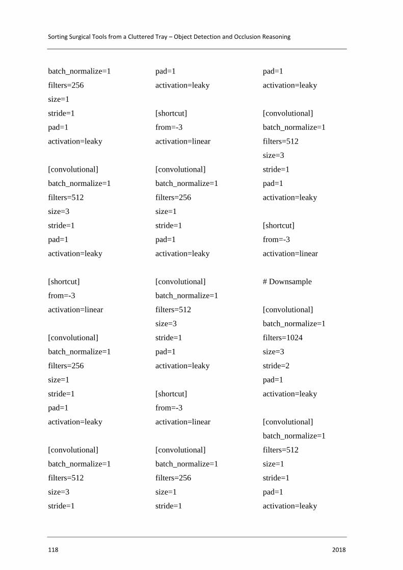
Sorting Surgical Tools from a Cluttered Tray – Object Detection and Occlusion Reasoning
118 2018
batch_normalize=1
filters=256
size=1
stride=1
pad=1
activation=leaky
[convolutional]
batch_normalize=1
filters=512
size=3
stride=1
pad=1
activation=leaky
[shortcut]
from=-3
activation=linear
[convolutional]
batch_normalize=1
filters=256
size=1
stride=1
pad=1
activation=leaky
[convolutional]
batch_normalize=1
filters=512
size=3
stride=1
pad=1
activation=leaky
[shortcut]
from=-3
activation=linear
[convolutional]
batch_normalize=1
filters=256
size=1
stride=1
pad=1
activation=leaky
[convolutional]
batch_normalize=1
filters=512
size=3
stride=1
pad=1
activation=leaky
[shortcut]
from=-3
activation=linear
[convolutional]
batch_normalize=1
filters=256
size=1
stride=1
pad=1
activation=leaky
[convolutional]
batch_normalize=1
filters=512
size=3
stride=1
pad=1
activation=leaky
[shortcut]
from=-3
activation=linear
# Downsample
[convolutional]
batch_normalize=1
filters=1024
size=3
stride=2
pad=1
activation=leaky
[convolutional]
batch_normalize=1
filters=512
size=1
stride=1
pad=1
activation=leaky

ANNEX A
Diana Martins Lavado 119
[convolutional]
batch_normalize=1
filters=1024
size=3
stride=1
pad=1
activation=leaky
[shortcut]
from=-3
activation=linear
[convolutional]
batch_normalize=1
filters=512
size=1
stride=1
pad=1
activation=leaky
[convolutional]
batch_normalize=1
filters=1024
size=3
stride=1
pad=1
activation=leaky
[shortcut]
from=-3
activation=linear
[convolutional]
batch_normalize=1
filters=512
size=1
stride=1
pad=1
activation=leaky
[convolutional]
batch_normalize=1
filters=1024
size=3
stride=1
pad=1
activation=leaky
[shortcut]
from=-3
activation=linear
[convolutional]
batch_normalize=1
filters=512
size=1
stride=1
pad=1
activation=leaky
[convolutional]
batch_normalize=1
filters=1024
size=3
stride=1
pad=1
activation=leaky
[shortcut]
from=-3
activation=linear
####################
##
[convolutional]
batch_normalize=1
filters=512
size=1
stride=1
pad=1
activation=leaky
[convolutional]
batch_normalize=1
size=3
stride=1
pad=1
filters=1024
activation=leaky
[convolutional]
batch_normalize=1
filters=512
size=1
stride=1

Sorting Surgical Tools from a Cluttered Tray – Object Detection and Occlusion Reasoning
120 2018
pad=1
activation=leaky
[convolutional]
batch_normalize=1
size=3
stride=1
pad=1
filters=1024
activation=leaky
[convolutional]
batch_normalize=1
filters=512
size=1
stride=1
pad=1
activation=leaky
[convolutional]
batch_normalize=1
size=3
stride=1
pad=1
filters=1024
activation=leaky
[convolutional]
size=1
stride=1
pad=1
filters=27
activation=linear
[yolo]
mask = 6,7,8
anchors = 10,13, 16,30,
33,23, 30,61, 62,45,
59,119, 116,90,
156,198, 373,326
classes=4
num=9
jitter=.3
ignore_thresh = .5
truth_thresh = 1
random=1
[route]
layers = -4
[convolutional]
batch_normalize=1
filters=256
size=1
stride=1
pad=1
activation=leaky
[upsample]
stride=2
[route]
layers = -1, 61
[convolutional]
batch_normalize=1
filters=256
size=1
stride=1
pad=1
activation=leaky
[convolutional]
batch_normalize=1
size=3
stride=1
pad=1
filters=512
activation=leaky
[convolutional]
batch_normalize=1
filters=256
size=1
stride=1
pad=1
activation=leaky
[convolutional]
batch_normalize=1
size=3
stride=1
pad=1
filters=512
activation=leaky

ANNEX A
Diana Martins Lavado 121
[convolutional]
batch_normalize=1
filters=256
size=1
stride=1
pad=1
activation=leaky
[convolutional]
batch_normalize=1
size=3
stride=1
pad=1
filters=512
activation=leaky
[convolutional]
size=1
stride=1
pad=1
filters=27
activation=linear
[yolo]
mask = 3,4,5
anchors = 10,13, 16,30,
33,23, 30,61, 62,45,
59,119, 116,90,
156,198, 373,326
classes=4
num=9
jitter=.3
ignore_thresh = .5
truth_thresh = 1
random=1
[route]
layers = -4
[convolutional]
batch_normalize=1
filters=128
size=1
stride=1
pad=1
activation=leaky
[upsample]
stride=2
[route]
layers = -1, 36
[convolutional]
batch_normalize=1
filters=128
size=1
stride=1
pad=1
activation=leaky
[convolutional]
batch_normalize=1
size=3
stride=1
pad=1
filters=256
activation=leaky
[convolutional]
batch_normalize=1
filters=128
size=1
stride=1
pad=1
activation=leaky
[convolutional]
batch_normalize=1
size=3
stride=1
pad=1
filters=256
activation=leaky
[convolutional]
batch_normalize=1
filters=128
size=1
stride=1
pad=1
activation=leaky
[convolutional]
batch_normalize=1
size=3
stride=1
pad=1

Sorting Surgical Tools from a Cluttered Tray – Object Detection and Occlusion Reasoning
122 2018
filters=256
activation=leaky
[convolutional]
size=1
stride=1
pad=1
filters=27
activation=linear
[yolo]
mask = 0,1,2
anchors = 10,13, 16,30,
33,23, 30,61, 62,45,
59,119, 116,90,
156,198, 373,326
classes=4
num=9
jitter=.3
ignore_thresh = .5
truth_thresh = 1
random=1

Erro! A origem da referência não foi encontrada.
Diana Martins Lavado 123
ANNEX C
Code adapted from AlexeyAB darknet repository to obtain the data for precision-
recall curve.
void validate_detector_PRcurve(char *datacfg, char *cfgfile, char *weightfile) { list *options = read_data_cfg(datacfg); char *valid_images = option_find_str(options, "valid", "Dataset-top-scalpel/test.txt"); network *net = load_network(cfgfile, weightfile, 0); set_batch_network(&net, 1); fprintf(stderr, "Learning Rate: %g, Momentum: %g, Decay: %g\n", net->learning_rate, net->momentum, net->decay); srand(time(0)); list *plist = get_paths(valid_images); char **paths = (char **)list_to_array(plist); layer l = net->layers[net->n-1]; int classes = l.classes; int j, k; box *boxes = calloc(l.w*l.h*l.n, sizeof(box)); float **probs = calloc(l.w*l.h*l.n, sizeof(float *)); for(j = 0; j < l.w*l.h*l.n; ++j) probs[j] = calloc(classes+1, sizeof(float *)); int m = plist->size; int i=0; float iou_thresh = .5; float nms = .4; for(float thresh = 0; thresh < 1; thresh = thresh + 0.01){ int total = 0; int TP = 0, FP = 0; int proposals = 0; float avg_iou = 0; for(i = 0; i < m; ++i){ char *path = paths[i]; image orig = load_image_color(path, 0, 0); image sized = resize_image(orig, net->w, net->h); char *id = basecfg(path); network_predict(net, sized.data); get_region_boxes(l, sized.w, sized.h, net->w, net->h, thresh, probs, boxes, 1, 0, .5, 1); if (nms) do_nms(boxes, probs, l.w*l.h*l.n, 1, nms); char labelpath[4096];

Sorting Surgical Tools from a Cluttered Tray – Object Detection and Occlusion Reasoning
124 2018
find_replace(path, "images", "labels", labelpath); find_replace(labelpath, "JPEGImages", "labels", labelpath); find_replace(labelpath, ".png", ".txt", labelpath); find_replace(labelpath, ".jpg", ".txt", labelpath); find_replace(labelpath, ".JPEG", ".txt", labelpath); int num_labels = 0; box_label *truth = read_boxes(labelpath, &num_labels); for(k = 0; k < l.w*l.h*l.n; ++k){ if(probs[k][0] > thresh){ ++proposals; } } for (j = 0; j < num_labels; ++j) { ++total; box t = {truth[j].x, truth[j].y, truth[j].w, truth[j].h}; float best_iou = 0; for(k = 0; k < l.w*l.h*l.n; ++k){ float iou = box_iou(boxes[k], t); if(probs[k][0] > thresh && iou > best_iou){ best_iou = iou; } } avg_iou += best_iou; if(best_iou > iou_thresh){ ++TP; } } FP = proposals - TP; free(id); free_image(orig); free_image(sized); } fprintf(stderr, "Thresh:%.4f\tRecall:%.2f%%\tPrecision:%.2f%%\n", thresh, 100.*TP/total, 100.*TP/(TP+FP)); } }