sound and ultrasound source direction …ecasp.ece.iit.edu/publications/thesis/vitaliy kunin...
TRANSCRIPT

SOUND AND ULTRASOUND SOURCE DIRECTION OF ARRIVAL ESTIMATION
AND LOCALIZATION
BY
VITALIY KUNIN
DEPARTMENT OF ELECTRICAL AND COMPUTER ENGINEERING
Submitted in partial fulfillment of the requirements for the degree of
Master of Science in Electrical Engineering in the Graduate College of the Illinois Institute of Technology
Approved _________________________ Adviser
Chicago, Illinois December 2010


iii
ACKNOWLEDGEMENT
I would like to express my gratitude to my thesis advisor Dr. Jafar Saniie for
encouraging and challenging me and for providing a great learning experience over the
course of my undergraduate and graduate education. I would also like to thank my
research lab colleagues and friends, Marcos, Alireza, Richard, and Vijay, for all the
technical advice they have given me throughout my graduate work.
I would like to express my gratitude to my family for all the support they provided
over the many years of education. I would like to thank my father, Vladimir, whose
technical expertise and assistance was a great help in many parts of this work. I would
like to thank my mother, Svetlana for her support and encouragement during all of my
education. I would also like to thank my sister, Alina, and brother in-law, Dmitriy, for
their support and encouragement.
iv
TABLE OF CONTENTS
Page
ACKNOWLEDGEMENT ....................................................................................... iii
LIST OF TABLES ................................................................................................... vi
LIST OF FIGURES ................................................................................................. vii
ABSTRACT ............................................................................................................. ix
CHAPTER
1. INTRODUCTION .................................................................................. 1
1.1 Motivation ................................................................................. 1 1.2 Objectives and Contributions .................................................... 3
2. THEORETICAL BACKGROUND ....................................................... 4
2.1 2D DOAE .................................................................................. 6 2.2 3D DOAE .................................................................................. 10 2.3 2D Localization ......................................................................... 13 2.4 3D Localization ......................................................................... 17 2.5 Ultrasound DOAE and Localization ......................................... 23 2.6 DOAE and Localization Restrictions and Considerations ........ 24 2.7 Matched Filters ......................................................................... 27
3. MICROPHONE ARRAY DATA ACQUISITION SYSTEM .............. 30
3.1 Introduction ............................................................................... 30 3.2 CAPTAN Architecture ............................................................. 32 3.3 Node Processing and Control Board (NPCB) ........................... 39 3.4 Gigabit Ethernet Link (GEL) Board ......................................... 42 3.5 Acoustic MEMS Array (AMA) ................................................ 44 3.6 Restrictions and Considerations ................................................ 49 3.7 Advantages ................................................................................ 51
4. GENERAL DATA ACQUISITION AND GENERATION .................. 53
4.1 Oscilloscope Based Data Acquisition ....................................... 53 4.2 Arbitrary Waveform Based Data Generation ........................... 59
v
5. ACOUSTIC CHAMBER, MEASUREMENT MOUNT AND SENSOR ARRAY TEST STAND ........................................................ 64
5.1 Acoustic Chamber ..................................................................... 64 5.2 Measurement Mount ................................................................. 72 5.3 Sensor Array Test Stand ........................................................... 74
6. AUXILIARY CIRCUITS AND SENSORS .......................................... 78
6.1 Auxiliary Circuits ..................................................................... 78 6.2 Sensors ...................................................................................... 80
7. EXPERIMENTS .................................................................................... 83
7.1 Sound Source Direction of Arrival Estimation (DOAE) .......... 83 7.2 Ultrasound Matched Filter ......................................................... 94 7.3 Ultrasound Object Imaging in Air .............................................. 105 7.4 Ultrasound Localization .............................................................. 108
8. CONCLUSION AND FUTURE WORK ................................................ 115
8.1 Conclusion ............................................................................. 115 8.2 Future Work ........................................................................... 118
BIBLIOGRAPHY .................................................................................................... 120
vi
LIST OF TABLES
Table Page
7.1 Sound Source DOAE Experiment Set 1, Outer Microphones Results ............ 87 7.2 Sound Source DOAE Experiment Set 1, Inner Microphones Results ............. 87 7.3 Sound Source DOAE Experiment Set 2, Outer Microphones Results ............ 88 7.4 Sound Source DOAE Experiment Set 2, Inner Microphones Results ............. 89 7.5 Sound Source DOAE Experiment Set 3 Results .............................................. 91 7.6 Sound Source DOAE Experiment Set 4 Results .............................................. 93 7.7 Volleyball Image Shadow Power Levels .......................................................... 107 7.8 Distances between the Receivers and the Transmitter for the 2D Setup ......... 110 7.9 Distances Corresponding to the TDOA Information for the 2D Setup ........... 110 7.10 Transmitter Coordinates Based on Distances for the 2D Setup ..................... 111 7.11 Transmitter Coordinates Based on TDOA for the 2D Setup ......................... 111 7.12 Distances between the Receivers and the Transmitter for the 3D Setup ....... 113 7.13 Distances Corresponding to the TDOA Information for the 3D Setup ......... 113 7.14 Transmitter Coordinates Based on Distances for the 3D Setup ..................... 114 7.15 Transmitter Coordinates Based on TDOA for the 3D Setup .......................... 114

vii
LIST OF FIGURES
Figure Page
2.1 DOA Geometry Top View ............................................................................... 6 2.2 DOA Far-Field Model ...................................................................................... 7 2.3 DOA Near-Field Model ................................................................................... 9 2.4 DOA Geometry Isometric View ...................................................................... 11 2.5 3D DOA Using 3 Receivers ............................................................................. 12 2.6 3D DOA Using 4 Receivers ............................................................................. 13 2.7 2D Localization Geometry Type 1 .................................................................. 14 2.8 2D Localization Geometry Type 2 .................................................................. 16 2.9 3D Localization Using Three Receivers Type 1 ............................................... 18 2.10 3D Localization Using Three Receivers Type 2 ............................................. 20 2.11 3D Localization Using Four Receivers .......................................................... 20 2.12 3D Localization Using Five Receivers .......................................................... 22 2.13 Spatial Aliasing Illustration ........................................................................... 25 2.14 Closed Form Solution Example ..................................................................... 27 2.15 No Closed Form Solution Examples .............................................................. 27 2.16 Matched Filter Template Sample ................................................................... 28 2.17 Matched Filter Template Sample with AWGN ............................................. 29 3.1 Picture of the Microphone Array Data Acquisition System ............................ 31 3.2 Functional Block Diagram of the Microphone Array Data Acquisition System ....................................................................... 31 3.3 CAPTAN Electrical Vertical Bus Connector .................................................. 32 3.4 CAPTAN System Board Top Layout View ..................................................... 36
viii
3.5 Top View Picture of the NPCB ....................................................................... 42 3.6 GEL Board Transfer Rate Graph ..................................................................... 43 3.7 Top View Picture of the GEL Board ............................................................... 44 3.8 Top View Picture of the AMA Board .............................................................. 45 3.9 SPM0208HE5 Frequency Response ................................................................ 46 3.10 SPM0204UD5 Frequency Response .............................................................. 47 3.11 MEMS Amplification and Filtering Circuit ................................................... 48 5.1 Outside of View of the Acoustic Chamber from the Top ................................ 65 5.2 Outside of View of the Acoustic Chamber from the Side ............................... 65 5.3 Inside of View of the Acoustic Chamber from the Top ................................... 66 5.4 Inside of View of the Acoustic Chamber from the Side .................................. 66 5.5 Acoustic Chamber Floor Cushion .................................................................... 69 5.6 Acoustic Chamber Ceiling Tiles Front and Back ............................................ 69 5.7 Acoustic Chamber Side Tiles Front and Back ................................................. 70 5.8 Acoustic Foam Absorption VS. Frequency ..................................................... 71 5.9 Measurement Mount Front View ..................................................................... 73 5.10 Measurement Mount Side View .................................................................... 73 5.11 Sensor Array Test Stand Front View ............................................................. 74 5.12 Sensor Directionality ..................................................................................... 76 5.13 Sensor Array Test Stand Rear View .............................................................. 77 6.1 Auxiliary Microphone Circuit .......................................................................... 79 6.2 Auxiliary Ultrasound Sensor Circuit ............................................................... 80 6.3 125KHF25 Beam Angle versus Attenuation ................................................... 81
ix
6.4 125KHF25 Frequency Response ..................................................................... 81 6.5 US40KT-01 Beam Angle versus Attenuation .................................................. 82 6.6 US40KT-01 Frequency Response .................................................................... 82 7.1 Sound Source DOAE Setup ............................................................................. 84 7.2 Sample Data Collected by MEMs Microphone Array ..................................... 85 7.3 Zoomed in Data Collected by Two MEMs Microphones ................................ 85 7.4 Microphones Used ........................................................................................... 86 7.5 Reflections from Microphone Array ................................................................ 90 7.6 Sound Source DOAE Experiment Set 4 Sample Results ................................. 92 7.7 Original Matlab Signal for the First Modulation Scheme ............................... 96 7.8 Measured Output of the Transmitter for the First Modulation Scheme ............................................................................................................. 96 7.9 Measured Received Signal for the First Modulation Scheme ......................... 97 7.10 Autocorrelation of the Transmitted Signal for the First Modulation Scheme ............................................................................................................ 97 7.11 Cross-Correlation between the Transmitted and Received Signal for the Modulation Scheme ........................................................................................ 98 7.12 Original Matlab Signal for the Second Modulation Scheme ......................... 99 7.13 Measured Output of the Transmitter for the Second Modulation Scheme .... 99 7.14 Measured Received Signal for the Second Modulation Scheme ................... 100 7.15 Autocorrelation of the Transmitted Signal for the Second Modulation Scheme ........................................................................................................... 100 7.16 Cross-Correlation between the Transmitted and Received Signal for the the Second Modulation Scheme ..................................................................... 101 7.17 Cross-Correlations between the Transmitted Signals of the Two Schemes ... 103
x
7.18 Cross-Correlation between the Transmitted Signal of the First Scheme and the Received Signal of the Second Scheme ............................................ 103 7.19 Cross-Correlation between the Transmitted Signal of the Second Scheme and the Received Signal of the First Scheme ................................................. 104 7.20 Cross-Correlation between the Transmitted Second Scheme and a Received Combination of the First and Second Schemes .............................. 104 7.21 Volleyball Imaging Setup .............................................................................. 106 7.22 Volleyball Imaging Shadow Raw Data .......................................................... 107 7.23 Volleyball Imaging Shadow Interpolated Data .............................................. 107 7.24 2D Ultrasound Localization Setup ................................................................. 109 7.25 3D Ultrasound Localization Setup ................................................................. 112
xi
ABSTRACT
Localization of sources and the detection of objects using ultrasound has been the
topic of a great deal of research as there are numerous applications for these techniques.
Some of the prominent applications of sound source localization are the enhancement of
human speech recognition for hands free man machine interface, the separation of
multiple sound sources for teleconferencing and the detection and localization of
mechanical or structural failures in vehicles and building or bridges. Ultrasound source
detection can also be used for the above described applications as well as for a wide
variety of security systems and for robotic vision.
This work explores the fundamentals of sound and ultrasound source localization
as well as ultrasound object imaging and matched filtering. The main parts of this work
are the design of an acoustic chamber, measurement mound, and sensor arrays, the
exploration of various sound and ultrasound acquisition systems, and the analysis of how
the acquired data could be used for sound source and object detection. The acoustic
chamber is used to create a clean environment which isolates the experiment from
external noises and reduces reverberation. The measurement mount is used to accurately
position the source. The sensor arrays are used to experiment with different geometries
and with different numbers of sensors. The acquisition systems explored include a novel
standalone field-programmable gate array (FPGA) micro-electro mechanical
microphones (MEMS) array system and various acquisition systems consisting of
independent circuits, components, and test equipment. The circuits considered are the
microphone and ultrasound transducer amplification and filtering circuit. Pertinent
modern test equipment, such as digital oscilloscopes and arbitrary waveform generators,

xii
and their features which are related to acquisition and generation of data are also
explained. This work concludes by discussing how several sound and ultrasound
localization, matched filtering, and ultrasound imaging experiments were conducted and
what the results of those experiments were.
1
CHAPTER 1
INTRODUCTION
1.1 Motivation
There is currently an enormous amount of research and applications which use
sound and ultrasound detection and analysis. Some of the research topics of sound
detection and analysis are sound source localization, sound source tracking, identification
of multiply sound sources, separation of multiple sound sources, acoustic scene analysis
and sensor network technology [Ben08, Bra01, Hyv00, Hyv01 Ran03, Tur10]. These
techniques have a wide variety of applications such as teleconferencing, multi-party
telecommunications, hands-free acoustic human-machine interfaces, computer games,
dictation systems, hearing-aids, and many more [Alg08, Ben08, Bra01, Tur10, Wan96].
Similarly there is myriad of research concerning the use of ultrasound detection and
analysis. Some of the prominent topics which use ultrasound are material analysis both
organic and non organic, air and water security and surveillance systems, and air and
water robotic vision systems. The applications of ultrasound material analysis include
medical diagnostics, structural failure analysis of buildings or bridges, and mechanical
failure analysis of machines such as vehicles or aircrafts. Robotic vision has applications
in robotic automation, these could be for home use systems such as an automated
appliances, industrial use such as assembly lines, and military use such as automated
aiming and guidance systems [Har08, Li06, Lla01, Nel08, Wel06].
While all of the above topics and applications may seem straightforward from a
theoretical and mathematical perspective in practice there are a large number of issues
encountered in a real environment which make realistic application of the theory
2
significantly more difficult [Ben08, Bra01, Gri02]. The most obvious problem when
working with sound and ultrasound is noise. Noise can either be ambient sound e.g.
computer fans, background discussions, ambient ultrasound noise e.g. lights, or electrical
noise of the sound/ultrasound acquisition system. Another difficulty when working with a
variety of sources like human speech is that speech is a wideband non-stationary signal,
i.e. it contains a broad range of frequencies and that range changes with time. Yet another
difficulty with both sound and ultrasound is reverberation or echoes. This is a significant
issue since echoes have the same spectral content as the original signal of interest. When
using highly directional ultrasound this issue is somewhat less significant since the type
signal does not scatter as much as sound, however this issues is still present when using
omni-directional ultrasound transmitters. Another issue encounter when using ultrasound
is its high frequency which requires higher speed systems and prevents the use of some
algorithms which could be used for sound this happens because the error due to sound
propagation becomes significant when compared to the frequency and phase of
ultrasound.
3
1.2 Objectives and Contributions
The objectives and contributions of this work are the following:
The exploration of the basic geometry and mathematics behind source
direction of arrival estimation and localization.
The exploration of ultrasound based matched filtering.
The exploration of ultrasound based object imaging.
The exploration of different sound and ultrasound acquisition methods
including a novel self-sufficient FPGA, MEMS based system and a
general oscilloscope based acquisition system with its associated circuitry.
The design of an anechoic chamber and measurement mount which would
allow for a controlled experimental setup for the exploration of the various
sound and ultrasound topics while accurately varying parameters such as
noise reverberation, distance, and angles.
Design of adjustable sensor arrays which would allow source localization
to be explored with a variety of sensor geometries and a variety of sound
and ultrasound sensors.
The exploration of source localization and object detection techniques
which could be applied to the acquired sound and ultrasound data.
4
CHAPTER 2
THEORETICAL BACKGROUND
Sound and ultrasound source localization is the process of determining the
position of an acoustic source, such as a human speaker, a stereo system speaker, or an
ultrasound transducer using two or more receivers or microphones. A similar but separate
topic is direction of arrival estimation (DOAE) which only determines the direction of the
sound source but not the distance to it [Ben08, Tel07]. Both localization and DOAE can
be broken down into several types. One distinction that can be made is whether 2
dimensional (2D) source localization and DOAE or 3 dimensional (3D) localization and
DOA is being performed. This simply refers to only looking for a sound source in a
plane, i.e. only horizontally or vertically, or in full 3D space. Yet another consideration of
source localization is whether near-field or far-field modeling is being used [Ben08,
McC01, Zio00]. Additionally source localization can be categorized by the type of
information used to perform the localization namely delays between the source’s transmit
time and receivers’ pickup times, delays between only the receivers’ pickup times called
time difference of arrival (TDOA), or power based localization. In this work the first two
sets of information are used as the power based methods are not sensitive enough for
accurate estimations when using a passive system.
Localization and DOAE approaches can also be separated by the type of source
signal being used, which could be continuous or pulse based, single amplitude or multiple
amplitude, and single frequency or multiple frequency (in this work only single
amplitude and single frequency source signals are used). Lastly localization and DOAE
can be separated by the type of TDOA and power based algorithms being used. For pulse
5
based signals the TDOA algorithm could be a threshold value detector which determines
at which point a signal was transmitted or received. For continuous signals where phase
is used the TDOA algorithm could be standard cross correlation, phase transform general
cross correlation, or other algorithms [Ben08, Bra01, Gri02. Mun03, Tel07].
Independent of the type of approached used both localization and DOAE can be
divided into three general steps: collecting data across multiple receivers and/or
transmitters, finding the phase difference and/or time difference of arrival, and
calculating the direction and possibly distance to the sound source. The two more
complex steps are finding the phase difference/TDOA and determining the
angle/distance. As stated earlier finding the difference/TDOA depends on the type of
algorithm used leading to a large number of approaches. Determining the angle and
distance from the phase information depends on the interpretation of the collected data
and depends on a large number of factors, discussed in detail later in the chapter, such as
source signal type, the model being used, the number of receivers that are used, whether
2D or 3D estimation is being performed, and whether DOAE or localization is being
performed.
All of the above considerations also apply to ultrasound source DOA estimation
and localization. However due to the high frequency of the source signal phase based
estimations cannot be directly used due to aliasing and pulse based ranging techniques
have to be used instead. Nonetheless methods have been developed to use a combination
of pulse based ranging techniques with phased based techniques for highly accurate
ultrasonic measurements [Que06].
6
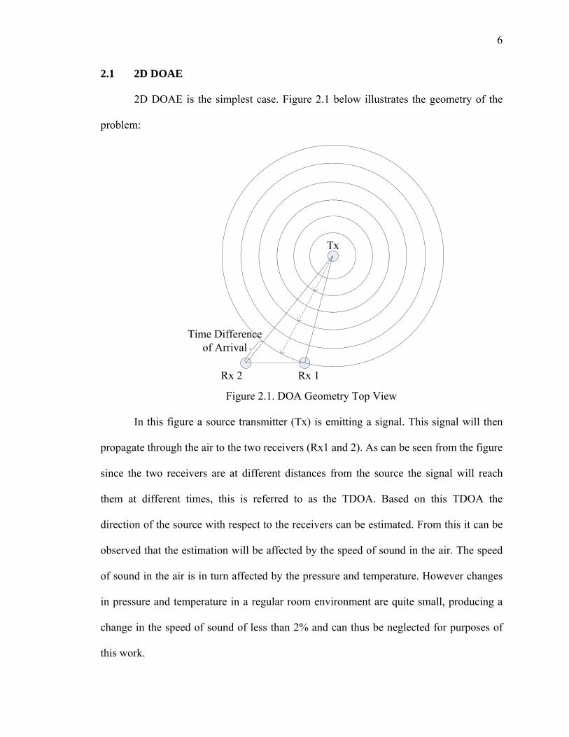
2.1 2D DOAE
2D DOAE is the simplest case. Figure 2.1 below illustrates the geometry of the
problem:
Tx
Rx 1Rx 2
Time Difference of Arrival
Figure 2.1. DOA Geometry Top View
In this figure a source transmitter (Tx) is emitting a signal. This signal will then
propagate through the air to the two receivers (Rx1 and 2). As can be seen from the figure
since the two receivers are at different distances from the source the signal will reach
them at different times, this is referred to as the TDOA. Based on this TDOA the
direction of the source with respect to the receivers can be estimated. From this it can be
observed that the estimation will be affected by the speed of sound in the air. The speed
of sound in the air is in turn affected by the pressure and temperature. However changes
in pressure and temperature in a regular room environment are quite small, producing a
change in the speed of sound of less than 2% and can thus be neglected for purposes of
this work.

7
The estimation of the direction can then be obtained through two models. The first
is the simplified far-field model [Ben08]. The far-field model assumes that the receivers
are far enough away from the source as to allow the spherical wave propagation shown in
figure 2.1 to be approximated by planes. This is similar to seeing the Earth as flat, thus if
the distance between the receivers is small compared to the distance between the
receivers and the transmitter the sound wave can be approximated to be a propagating
plane. This model is shown below in figure 2.2:
Figure 2.2. DOA Far-Field Model
In this model the angle that the source makes to the plane connecting the two
receivers is given by a, the distance between the receivers is d, and the distance
corresponding to the TDOA is T. At this point it should be noted that the TDOA is the
information that is directly obtained from the receivers and T is given by equation (2.1)
below:
T TDOA c (2.1)
Where c is the speed of sound, approximately 344m/s, and the TDOA is the delay
in seconds between the two received the signal. The inter-receiver distance is typically
8
known since it can be set or measured by the designer or user. From this model it can be
seen that the angle of the direction of the source to the receivers can be related to T and d
by equation 2.2 given below:
T cos a d (2.2)
Thus equation 2.3 below is the final equation which gives the direction of the
source:
angle acos T/d acos TDOA c/d (2.3)
A general model without approximations is called the near-field model, even
though it is correct for both sources that are close and far away from the receivers. This
model corresponds to using the real spherical wave propagation as shown in figure 2.1.
DOA estimation with this model however cannot be obtained from only the TDOA of
two receivers, instead this model requires the distances (or equivalently the time delays
between when the signal was transmitted and when it was received) from the source to
each of the receivers. If the distance to each receiver cannot be obtained the alternative is
to use three receivers which would allow DOA estimation using the near-field model and
only the TDOA information. This model is not very useful for DOAE since the
information or number of receivers used for this model allows localization to be
performed which is superior to DOA estimation as will be discuss later in section 2.3.
The mathematics behind DOA estimation using two receivers and the near-field model is
shown in figure 2.3 below:
9
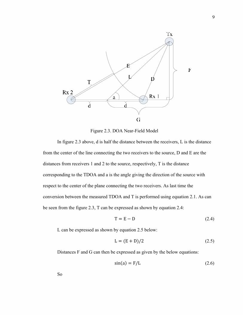
Figure 2.3. DOA Near-Field Model
In figure 2.3 above, d is half the distance between the receivers, L is the distance
from the center of the line connecting the two receivers to the source, D and E are the
distances from receivers 1 and 2 to the source, respectively, T is the distance
corresponding to the TDOA and a is the angle giving the direction of the source with
respect to the center of the plane connecting the two receivers. As last time the
conversion between the measured TDOA and T is performed using equation 2.1. As can
be seen from the figure 2.3, T can be expressed as shown by equation 2.4:
T E D (2.4)
L can be expressed as shown by equation 2.5 below:
L E D /2 (2.5)
Distances F and G can then be expressed as given by the below equations:
sin a F/L (2.6)
So
10
F sin a L (2.7)
And
cos a G/L (2.8)
So
G cos a L (2.9)
Now using the Pythagorean Theorem distance D can be expressed by equation
2.10 shown below:
D L cos a d L sin a (2.10)
Similarly distance E can be expressed by equation 2.11 shown below:
E L cos a d L sin a (2.11)
Plugging equations 2.1, 2.10 and 2.11 into equation 2.4 leads equation 2.12 which
is the final result, giving the relationship between the TDOA and the source angle:
TDOA c T E D
L cos a d L sin a L cos a d L sin a (2.12)
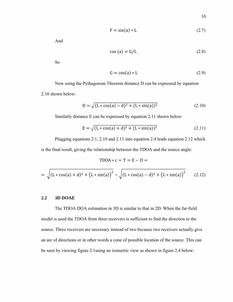
2.2 3D DOAE
The TDOA DOA estimation in 3D is similar to that in 2D. When the far-field
model is used the TDOA from three receivers is sufficient to find the direction to the
source. Three receivers are necessary instead of two because two receivers actually give
an arc of directions or in other words a cone of possible location of the source. This can
be seen by viewing figure 2.1using an isometric view as shown in figure 2.4 below:

11
Figure 2.4. DOA Geometry Isometric View
When performing 2D DOA estimation one of the planes is assumed to be fixed
thus the possible locations of the source is reduced to one which is in the plane of
interest.
In 3D DOA estimation any two pairs of the three receivers could be used to
determine two cones of possible points where the source could be. The location of where
these two cones intersect forms a line which gives the direction of the source.
Geometrically the three receivers being used have to be positioned in a plane i.e. not on a
line. This is because any two pairs of receivers on a line will give the same arc of
possible transmitter directions. One possible geometric arrangement of a three receiver
system for 3D DOA estimation is shown in figure 2.5 below:

12
Figure 2.5. 3D DOA Using 3 Receivers
In this figure the four angles shown in each diagram are equal and represent one
of the angles to the source in one of the three planes. Thus the mathematics used to
determine the 3D DOA is the same as that for 2D DOA estimation, only here the
operation needs to be performed twice for the two pairs of receivers and the results are
interpreted as giving the two angles of spherical coordinate system. As can be seen from
figure 2.5 when three receivers are used the two angles are centered on different points.
This however is negligible when the distance between the receivers is significantly
smaller then the distance to the source. Mathematically the result of using two different
center points is that the intersection of the two cones will form a parabola instead of a
line, however recalculating to compensate for the two different center points will again
give a line (i.e. direction) instead of a parabola. To avoid the issues associated with
having different center points a four receiver arrangement, with each pair being centered
on the same point as shown in figure 2.6 below, can be used:
13
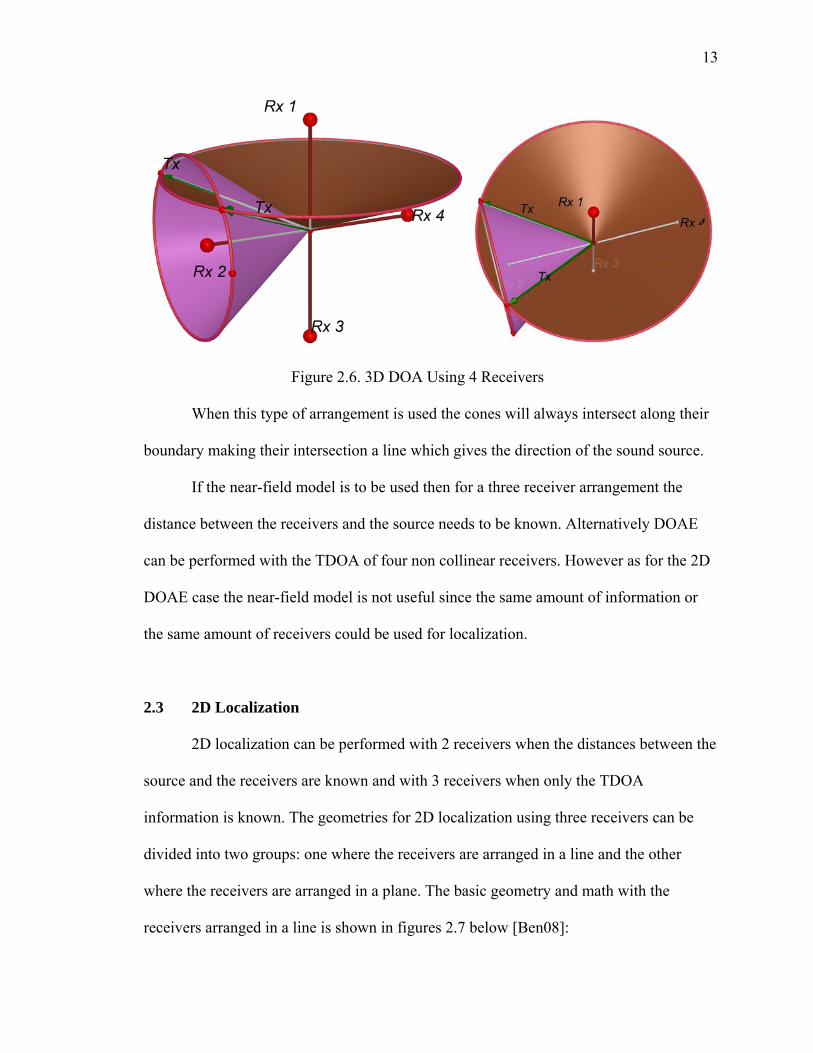
Figure 2.6. 3D DOA Using 4 Receivers
When this type of arrangement is used the cones will always intersect along their
boundary making their intersection a line which gives the direction of the sound source.
If the near-field model is to be used then for a three receiver arrangement the
distance between the receivers and the source needs to be known. Alternatively DOAE
can be performed with the TDOA of four non collinear receivers. However as for the 2D
DOAE case the near-field model is not useful since the same amount of information or
the same amount of receivers could be used for localization.
2.3 2D Localization
2D localization can be performed with 2 receivers when the distances between the
source and the receivers are known and with 3 receivers when only the TDOA
information is known. The geometries for 2D localization using three receivers can be
divided into two groups: one where the receivers are arranged in a line and the other
where the receivers are arranged in a plane. The basic geometry and math with the
receivers arranged in a line is shown in figures 2.7 below [Ben08]:
14
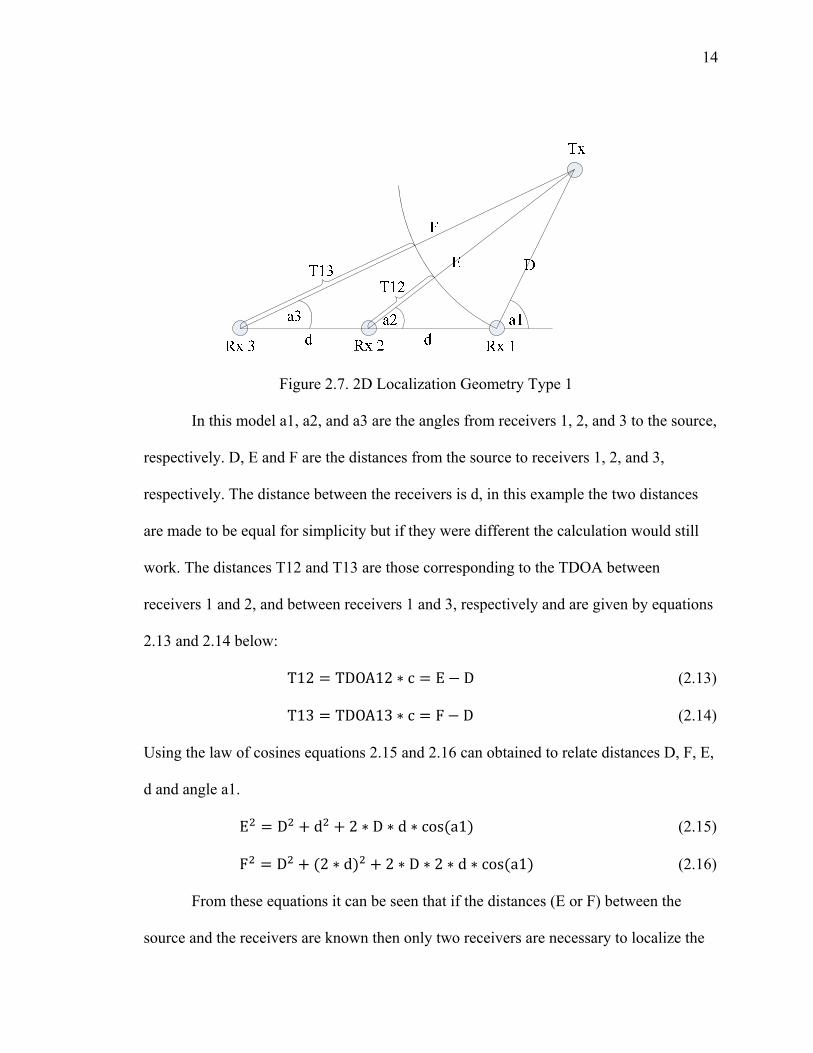
Figure 2.7. 2D Localization Geometry Type 1
In this model a1, a2, and a3 are the angles from receivers 1, 2, and 3 to the source,
respectively. D, E and F are the distances from the source to receivers 1, 2, and 3,
respectively. The distance between the receivers is d, in this example the two distances
are made to be equal for simplicity but if they were different the calculation would still
work. The distances T12 and T13 are those corresponding to the TDOA between
receivers 1 and 2, and between receivers 1 and 3, respectively and are given by equations
2.13 and 2.14 below:
T12 TDOA12 c E D (2.13)
T13 TDOA13 c F D (2.14)
Using the law of cosines equations 2.15 and 2.16 can obtained to relate distances D, F, E,
d and angle a1.
E D d 2 D d cos a1 (2.15)
F D 2 d 2 D 2 d cos a1 (2.16)
From these equations it can be seen that if the distances (E or F) between the
source and the receivers are known then only two receivers are necessary to localize the
15
source directly from one of the above equations. However if only the TDOA information
is given equations 2.13 and 1.14 need to be substituted into equations 2.15 and 2.16
leading to equation 2.17 and 2.18 below:
TDOA12 c D D d 2 D d cos a1 (2.17)
TDOA13 c D D 2 d 2 D 2 d cos a1 (2.18)
Equations 2.17 and 2.18 are two equations in two unknowns since the TDOA12
and the TDOA13 will be the collected data and d as well as c are known quantities. Using
equations 2.17 and 2.18 the variables D and a1 can be solved for. Next equations 2.13
and 2.14 can be used to solve for E and F. Now applying the cosine rule to triangle D, d,
E gives angle a2 and applying the cosine rule to triangle E, d, F gives angles a3. Thus as
can be seen the distance and angle from each receiver can be obtained. Solving equations
2.17 and 2.18 can be done through the use of a computer program but from this
derivation it can be observed that finding the distance and angle is computationally more
complex then only finding the direction. Alternatively to the above derivation, which uses
the law of cosines, two and three circle equations can be used for localization for the two
and three receivers on a line geometry similarly to how they are used in the next section
for receivers on a plane geometry.
The basic geometry and math with receivers arranged on a plane is shown in
figures 2.8 below, here the receivers are arranged in an equilateral triangle however this
is only to simplify the math and any triangle geometry would work. In this geometry it is
assumed that the source is located in-between the receivers.
16
d
d d
xy
r1 r2
r3
Tx
Rx 3
Rx 1 Rx 2
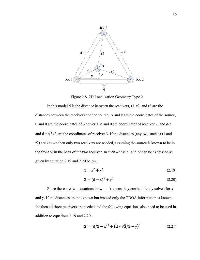
Figure 2.8. 2D Localization Geometry Type 2
In this model d is the distance between the receivers, r1, r2, and r3 are the
distances between the receivers and the source, x and y are the coordinates of the source,
0 and 0 are the coordinates of receiver 1, d and 0 are coordinates of receiver 2, and d/2
and d √3/2 are the coordinates of receiver 3. If the distances (any two such as r1 and
r2) are known then only two receivers are needed, assuming the source is known to be in
the front or in the back of the two receiver. In such a case r1 and r2 can be expressed as
given by equation 2.19 and 2.20 below:
r1 x y (2.19)
r2 d x y (2.20)
Since these are two equations in two unknowns they can be directly solved for x
and y. If the distances are not known but instead only the TDOA information is known
the then all three receivers are needed and the following equations also need to be used in
addition to equations 2.19 and 2.20.
r3 d/2 x d √3/2 y (2.21)
17
r3 r1 a (2.22)
r3 r2 b (2.23)
Here a and b the distances which correspond to the collected TDOA between the
three receivers. These are then five equations in five unknowns which could be solved to
obtain the x and y coordinates of the source as well as the distances between the receivers
and the transmitter.
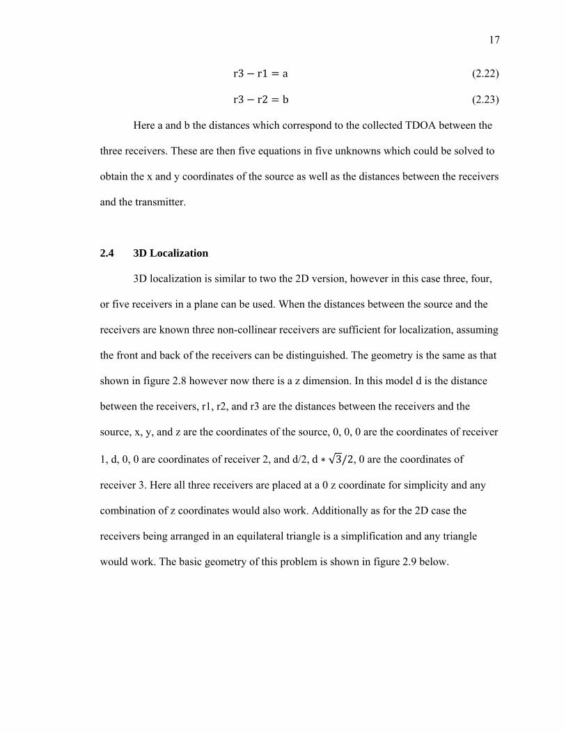
2.4 3D Localization
3D localization is similar to two the 2D version, however in this case three, four,
or five receivers in a plane can be used. When the distances between the source and the
receivers are known three non-collinear receivers are sufficient for localization, assuming
the front and back of the receivers can be distinguished. The geometry is the same as that
shown in figure 2.8 however now there is a z dimension. In this model d is the distance
between the receivers, r1, r2, and r3 are the distances between the receivers and the
source, x, y, and z are the coordinates of the source, 0, 0, 0 are the coordinates of receiver
1, d, 0, 0 are coordinates of receiver 2, and d/2, d √3/2, 0 are the coordinates of
receiver 3. Here all three receivers are placed at a 0 z coordinate for simplicity and any
combination of z coordinates would also work. Additionally as for the 2D case the
receivers being arranged in an equilateral triangle is a simplification and any triangle
would work. The basic geometry of this problem is shown in figure 2.9 below.
18
Figure 2.9. 3D Localization Using Three Receivers Type 1

19
The equations used for localization are three sphere equations where each sphere
is centered at the location of a receiver and has a radius equal to the distance between the
receiver and transmitter. These equations are given below:
r1 x y z (2.24)
r2 d x y z (2.25)
r3 d/2 x d √3/2 y z (2.26)
These are three equations in three unknowns thus allowing the x, y, and z
coordinates of the source to be determined. The reason that the three receivers must be
non-collinear is because three collinear spheres intersect in one circle instead of a point.
When the three receivers are non-collinear the three spheres intersect in two circles and
the two circles intersect at a point.
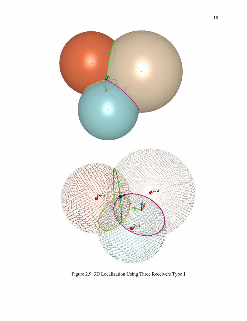
Alternatively if only the TDOA information is known and the distances between
the source and receivers are not known localization can be performed using the far-field
model estimation with three non-collinear receivers. This approach has the advantage of
using a small number of receivers however it is the most computationally and
conceptually complex, and is also a rougher estimation. In this case when three receivers
are used each pair of the receivers creates a cone giving the possible direction of the
source, the location of where these three cones intersect is then the location of source.
Since each pair of receivers does not center on the same point some recalculation is
required to get the distance and direction from a common center point. The three receiver
geometry is illustrated by figure 2.10 below:
20
Figure 2.10. 3D Localization Using Three Receivers Type 2
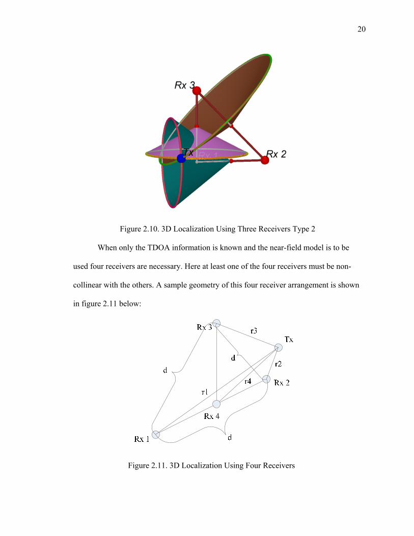
When only the TDOA information is known and the near-field model is to be
used four receivers are necessary. Here at least one of the four receivers must be non-
collinear with the others. A sample geometry of this four receiver arrangement is shown
in figure 2.11 below:
Figure 2.11. 3D Localization Using Four Receivers
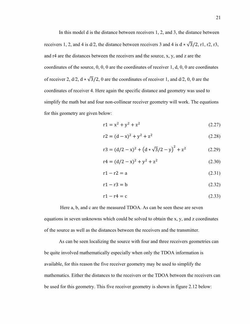
21
In this model d is the distance between receivers 1, 2, and 3, the distance between
receivers 1, 2, and 4 is d/2, the distance between receivers 3 and 4 is d √3/2, r1, r2, r3,
and r4 are the distances between the receivers and the source, x, y, and z are the
coordinates of the source, 0, 0, 0 are the coordinates of receiver 1, d, 0, 0 are coordinates
of receiver 2, d/2, d √3/2, 0 are the coordinates of receiver 1, and d/2, 0, 0 are the
coordinates of receiver 4. Here again the specific distance and geometry was used to
simplify the math but and four non-collinear receiver geometry will work. The equations
for this geometry are given below:
r1 x y z (2.27)
r2 d x y z (2.28)
r3 d/2 x d √3/2 y z (2.29)
r4 d/2 x y z (2.30)
r1 r2 a (2.31)
r1 r3 b (2.32)
r1 r4 c (2.33)
Here a, b, and c are the measured TDOA. As can be seen these are seven
equations in seven unknowns which could be solved to obtain the x, y, and z coordinates
of the source as well as the distances between the receivers and the transmitter.
As can be seen localizing the source with four and three receivers geometries can
be quite involved mathematically especially when only the TDOA information is
available, for this reason the five receiver geometry may be used to simplify the
mathematics. Either the distances to the receivers or the TDOA between the receivers can
be used for this geometry. This five receiver geometry is shown in figure 2.12 below:

22
Figure 2.12. 3D Localization Using Five Receivers
The way in which this five receiver geometry helps is by reducing one three
dimensional problem into several two dimensional problems. For the case in which only
the TDOA information is available, three receivers in each plane are used in the same
way that they were used for 2D localization type 1 shown in figure 2.7, with both results
using the same coordinate system centered at receiver 5. Since two planes are used all
information about the source is obtained. Geometrically this is the same as finding two
circles, or semi-circles, the intersection of which is the location of the sound source.
When the distances between the receivers and transmitter are known this
geometry again allows the three dimensional problem to be broken down into several two
dimensional problems. It should be noted however that the basis for this simplification in
this case is that the microphones form an L shape, the five receiver plus shape simply has

23
four L shapes providing redundancy and reducing error. Here again equations 2.15 and
2.16 are used to obtain the simplified solution.
2.5 Ultrasound DOAE and Localization
The main difference between sound and ultrasound source localization and DOA
estimation is that the frequency of ultrasound is too high to get the TDOA from the phase
information of the signals received by the ultrasound microphones. This occurs because
as frequency of the source signal gets higher its wavelength becomes smaller and the
required spatial distance between the microphones becomes shorter, as explained in
section 2.6. For example a 40 kHz ultrasound signal has a wavelength of 0.0086 meters
requiring a distance between the ultrasound microphones to be less than 4.3 millimeters.
This is physically challenging as most microphones will be too large to be placed this
close together and clearly any ultrasound frequency above 40 kHz will make the problem
worse. Additionally even if the ultrasound microphones could be placed this close
together the total maximum TDOA between them would be very small making the
system very prone to noise errors.
To avoid the above described issues ultrasound DOA estimation and localization
is based on using a train of pulses and then simply measuring the time difference between
when this train of pulses begins or ends at each microphone. This removes the
requirement of a maximum inter-microphone distance allowing more accurate
measurements to be made. Furthermore in this type of arrangement the further the
microphones are from each other the more accurate the localization and DOA estimation
will be.
24
2.6 DOAE and Localization Restrictions and Considerations
There are several restrictions present when dealing with the above described DOA
and distance estimation. When dealing with phase based experiments the most well
known is the temporal sampling theorem which states that the sampling rate of the
acquisition system must be at least double that of the highest frequency component of the
sound source signal [Pro07]. It should also be noted that while this is the minimum
requirement a sampling frequency of several times that of the maximum frequency
component of the source signal is desirable so that the collected data could be understood
from a visual inspection.
Another similar requirement for phase based experiments is the minimum spatial
sampling theorem [Ben08, McC01]. This is basically the same issue as the temporal
sampling theorem. This theorem states that for a given maximum temporal frequency in
the source signal there is a minimum spatial sampling, i.e. there is a maximum distance
between the receivers used in the acquisition system. Specifically this maximum distance
is given by equations 2.34 below:
d c 2 fmax⁄ λmin/2 (2.34)
Where d is the maximum distance between the receivers, c is the speed of sound,
fmax is the maximum frequency of the source signal, and λmin is minimum wavelength
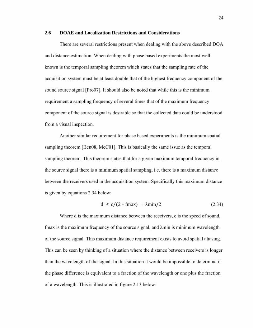
of the source signal. This maximum distance requirement exists to avoid spatial aliasing.
This can be seen by thinking of a situation where the distance between receivers is longer
than the wavelength of the signal. In this situation it would be impossible to determine if
the phase difference is equivalent to a fraction of the wavelength or one plus the fraction
of a wavelength. This is illustrated in figure 2.13 below:
25
Figure 2.13. Spatial Aliasing Illustration
Yet another issue with all of the above described estimations is that they actually
give two possible results one for the front of the systems of receivers and one for the
back. This is not a serious concern as we typically know which way our system is looking
and which general direction the source is. If these assumptions cannot be made another
receiver is needed for all of the above described configurations to determine whether the
source is in the back or the front of the system.
A key consideration is when localization can be performed and when the general
near-field model can be used [Ben08, McC01, Zio00]. While in a theoretically perfect
environment direction and distance estimation can be performed at any distance this does
not work in reality. In practice the source has to be sufficiently close to the receivers, i.e.
in the near-field. This occurs because the above described calculation depends on the
sound wave emanating from the source having a spherical nature when it reaches the
receivers. If the source is very far away the received sound wave will look like a plane,
shown in figure 2.2. When this occurs the angles from each receiver to the source will be
almost the same and the electronic noise error of the acquisition system, the error due to
26
acoustic noise, air temperature, and pressure variations will become large compared to
the actual difference between the angles, leading to incorrect estimations.
Another important matter that must be considered is that when DOAE and
localization are performed based on the receivers to transmitter distances the measured
distances will not be the same as the theoretically expected values. This is obvious,
however this results not only in measurement error but also in the lack of analytical
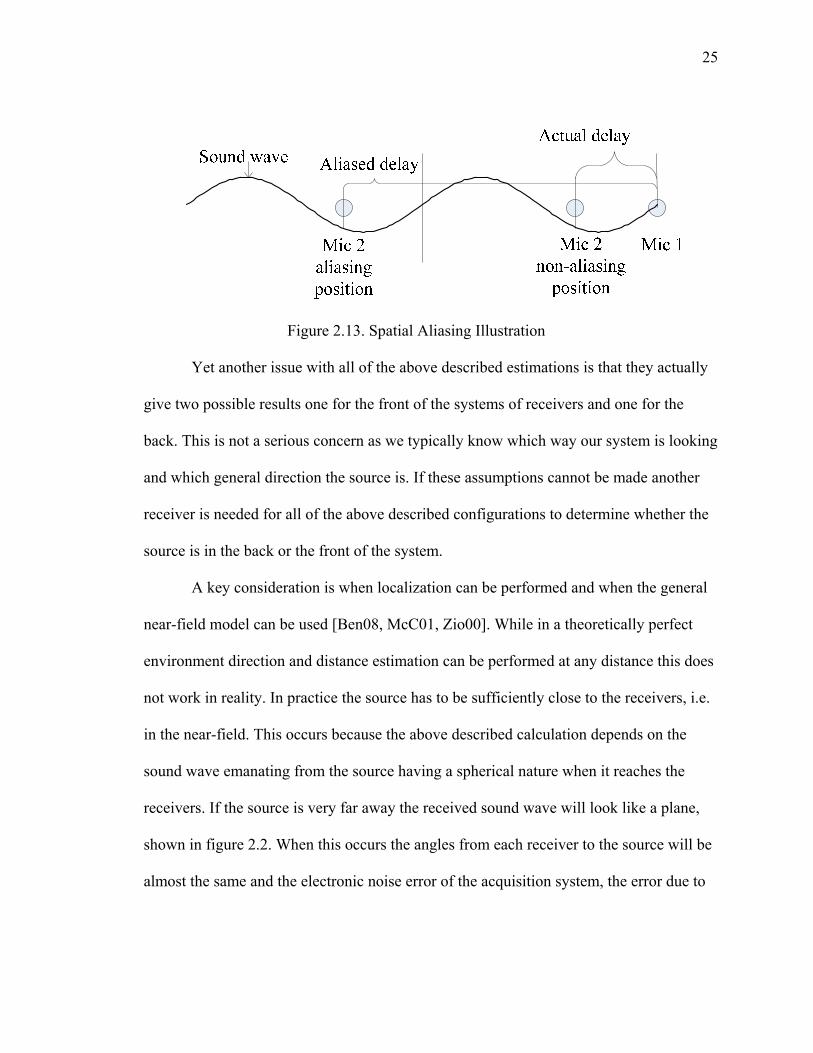
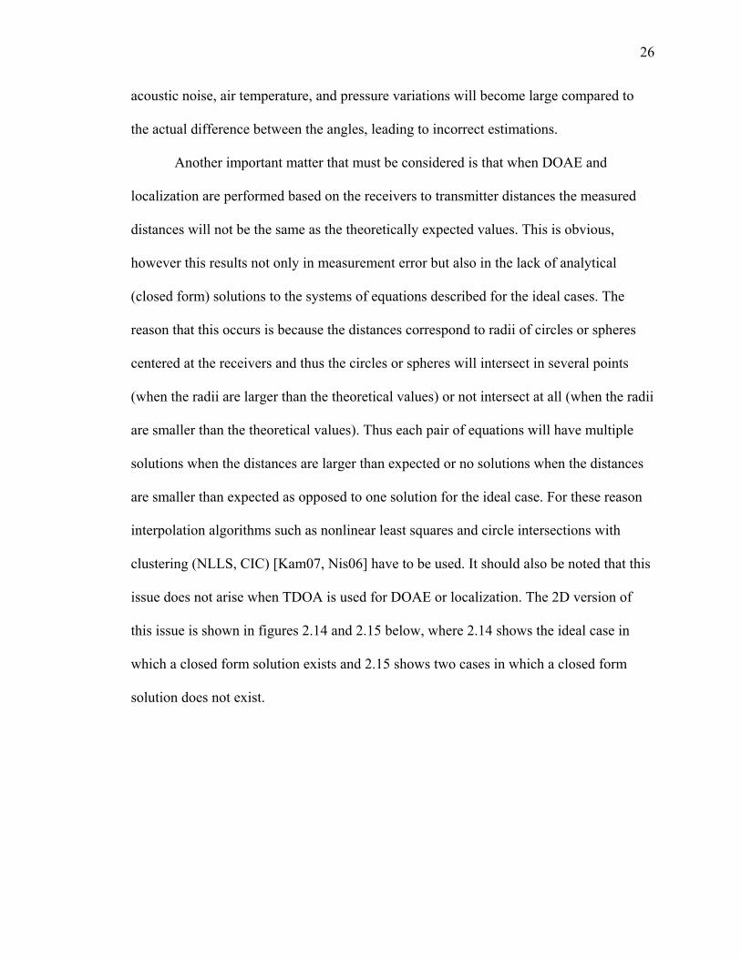
(closed form) solutions to the systems of equations described for the ideal cases. The
reason that this occurs is because the distances correspond to radii of circles or spheres
centered at the receivers and thus the circles or spheres will intersect in several points
(when the radii are larger than the theoretical values) or not intersect at all (when the radii
are smaller than the theoretical values). Thus each pair of equations will have multiple
solutions when the distances are larger than expected or no solutions when the distances
are smaller than expected as opposed to one solution for the ideal case. For these reason
interpolation algorithms such as nonlinear least squares and circle intersections with
clustering (NLLS, CIC) [Kam07, Nis06] have to be used. It should also be noted that this
issue does not arise when TDOA is used for DOAE or localization. The 2D version of
this issue is shown in figures 2.14 and 2.15 below, where 2.14 shows the ideal case in
which a closed form solution exists and 2.15 shows two cases in which a closed form
solution does not exist.
27
Figure 2.14. Closed Form Solution Example
Figure 2.15. No Closed Form Solution Examples
2.7 Matched Filters
Matched filtering is considered in this work as it is a technique which has two
main advantages for DOAE, localization, and ranging. The first advantage that matched
filtering provides is an improved accuracy of DOAE, localization, and ranging
estimations [Que06B]. Specifically matched filtering is used to increase the signal to
28
noise ratio (SNR) and thus increase reliability for transmitting and receiving information
in the presence of additive white Gaussian noise (AWGN). The second advantage that
matched filtering provides is the ability to transmit and receive several signals at the same
time over the same medium thus allowing the localization of multiple source at the same
time.
The technique works by using a known signal template for transmission and then
looking for this template at the receiving side of the communications. A key advantage of
the matched filter technique is that even if the original templates are mixed with noise or
with each other they can still be recovered and their position determined. Typically for
matched filtering a range of parameters such as frequency, individual segment duration,
overall duration for the template, amplitude, individual segment shape, and overall
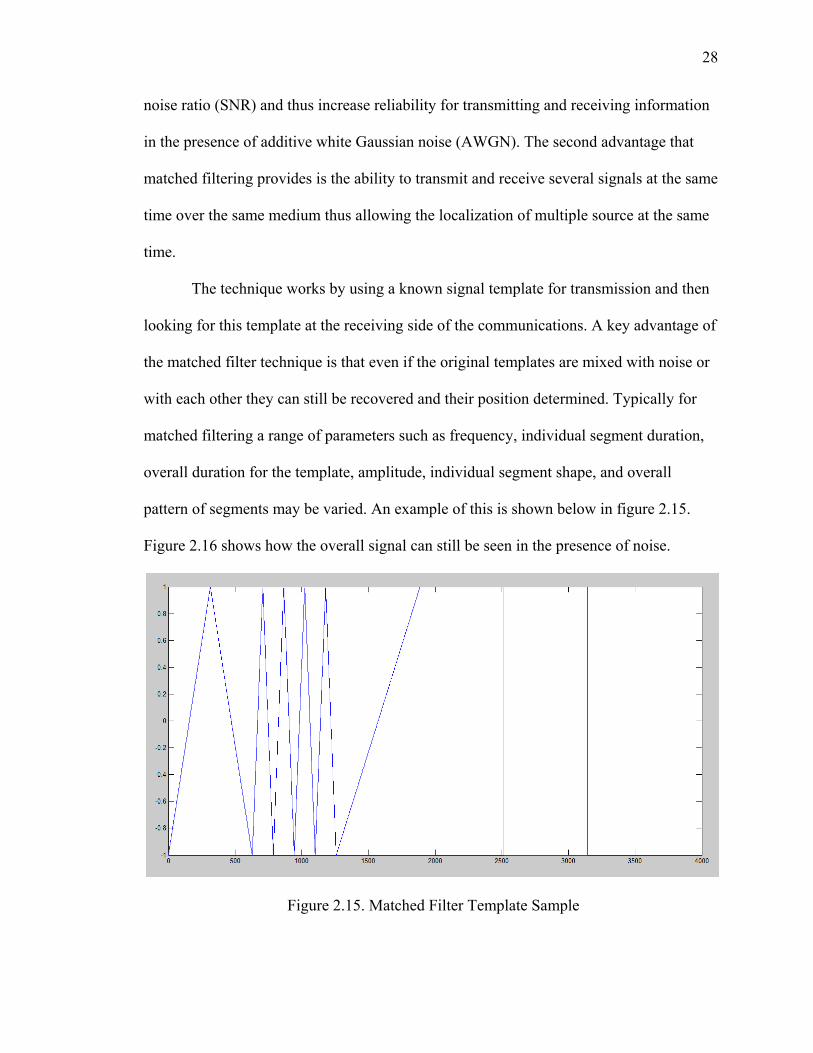
pattern of segments may be varied. An example of this is shown below in figure 2.15.
Figure 2.16 shows how the overall signal can still be seen in the presence of noise.
Figure 2.15. Matched Filter Template Sample

29
Figure 2.16. Matched Filter Template Sample with AWGN
30
CHAPTER 3
MICROPHONE ARRAY DATA ACQUISITION SYSTEM
3.1 Introduction
The microphone array data acquisition system (MADAS) used in this work is a
novel PC/FPGA based data acquisition system with an embedded MEMS based
microphone array. The data acquisition system is flexible, expandable, scalable, and has
both logging and real-time signal processing capability. More specifically the system can
collect data from 52 microphones simultaneously at sampling rates up to 300 Ksps
[Nat10, Tur10]. This data can be processed in real-time using the FPGA and then sent to
a PC or alternatively the raw unprocessed data can be sent to a PC. The system to PC
communications is performed through a gigabit Ethernet connection allowing high rates
of transfer for the massive amount of data. Multiply systems can be interconnected and
work in tandem through the use of standard hardware such as routers, making the system
highly expandable. Each system in a network of systems can be connected to a different
PC and different pieces of software of the system can run on different cores of a
processor making the system highly scalable [Tur10].
The system’s flexibility comes from the use of a central architecture called the
Compact And Programmable daTa Acquisition Node (CAPTAN). This architecture was
designed to be generally applicable to a variety of data acquisition problems and thus
uses standardized and modular hardware, configware, and software [Tur08].
Physically the system can be separated into three parts namely the Node
Processing and Control Board (NPCB), the Gigabit Ethernet Board (GEL), and the
Acoustic MEMS Array (AMA). The NPCB is the backbone board that contains the

31
FPGA which contains the system’s configware. The GEL board controls Ethernet
communications. The MEMS board is the hardware which contains the microphones,
amplifiers and analog to digital converters (ADC). Figure 3.1 below illustrates the three
hardware components that make up the system [Tur10].
Figure 3.1. Picture of the Microphone Array Data Acquisition System
Microphone Array Board
Microphones
Amplifiers and Filters
Analog to Digital
Converters
Node Processing and Control Board
FPGA
Gigabit Ethernet Board
PC
Gigabit Ethernet
Card
E2PROM
Figure 3.2. Functional Block Diagram of the Microphone Array Data Acquisition System

32
3.2 CAPTAN Architecture
The CAPTAN architecture is designed to support a distributed system which is
based on standalone pieces called nodes. Each node is made up of several interconnected
boards which have the capability of communicating with each other. An overall system
can in turn be made up of a single or multiple nodes which can also communicate with
each other. The CAPTAN architecture can be conceptually separated into three parts or
layers: the node layer, the network layer, and the application interface layer [Tur10].
The Node Layer. This layer can be subdivided into three main parts the vertical bus, the
horizontal bus, and the hardware boards. The vertical bus is a high speed, large bit width
bus responsible for the intra-node communications, i.e. board to board communication
within the same node. The vertical bus itself can also be subdivided into three parts: the
electrical vertical data transfer bus, electrical vertical system bus, and the optical vertical
data bus. The electrical vertical data bus is responsible for transferring data between the
node boards. The optical vertical data bus is also responsible for data transfer between the
boards in a node but allows even higher speeds. The electrical vertical system bus is
responsible for transferring control data between the boards in a node.
Physically the electrical vertical data and system bus share four connectors on the
top and bottom of each board. Using these connectors each board in a node is then
connected in a stack format. Alternately individual pins of the connectors could be used
for interfacing external circuits to the node. Each of the four connectors of the electrical
vertical bus consists of 64 pin data bus, a 16 pin data bus, and a 10 pin data bus for a total
of 12 data buses. Each of the vertical bus connectors also contains a 48 pin system
33
control bus and a 16 pin Serial Peripheral Interface (SPI) system control bus for a total of
8 system buses. Lastly the system power is also distributed through these vertical bus
connectors, providing unregulated voltages of 3.3V, 5.0V, 12V and -12V.
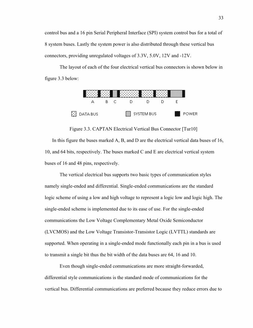
The layout of each of the four electrical vertical bus connectors is shown below in
figure 3.3 below:
Figure 3.3. CAPTAN Electrical Vertical Bus Connector [Tur10]
In this figure the buses marked A, B, and D are the electrical vertical data buses of 16,
10, and 64 bits, respectively. The buses marked C and E are electrical vertical system
buses of 16 and 48 pins, respectively.
The vertical electrical bus supports two basic types of communication styles
namely single-ended and differential. Single-ended communications are the standard
logic scheme of using a low and high voltage to represent a logic low and logic high. The
single-ended scheme is implemented due to its ease of use. For the single-ended
communications the Low Voltage Complementary Metal Oxide Semiconductor
(LVCMOS) and the Low Voltage Transistor-Transistor Logic (LVTTL) standards are
supported. When operating in a single-ended mode functionally each pin in a bus is used
to transmit a single bit thus the bit width of the data buses are 64, 16 and 10.
Even though single-ended communications are more straight-forwarded,
differential style communications is the standard mode of communications for the
vertical bus. Differential communications are preferred because they reduce errors due to

34
noise and electromagnetic coupling effects and allow a faster rate of transmission. The
standard used for differential communications is Low-Voltage Differential Signaling
(LVDS). It should also be noted that when operating in differential mode functionally the
bit width of each bus reduces to 32, 8, and 5 bits.
The optical vertical bus is another method of board to board data transfer in a
node. The optical interface uses lasers to serially transfer data at rates of up to 1 Gbps.
This transfer can be between any two boards in a node stack using the interface
independent of the distance between the boards and number of boards being used.
The physical location of the optical transmitters is in the corner of the board in
between the electrical vertical bus connectors. For this bus to be used each board in the
node stack must either have an optical transceiver in this position or a window. Of course
if a certain board uses a window this is only to allow other boards in the stack to use the
optical bus as the board with the window will not be able to use it.
The system bus can be divided into two parts the system control bus and the
system SPI bus. The system control bus is used by the system arbitration configware of
each node to make sure that critical control information, such as the status of the data
buses, gets transmitted without being blocked by lower priority signals. The system SPI
bus is used to transfer the configware to various programmable components on a
CAPTAN node. The system control bus also contains a 33MHz reference clock, the node
hardware reset signal, and spare pins for future expansion of CAPTAN system.
Together the system bus arbitration configware and the SPI configware are called
the system bus controller which is located on an NPCB board. For this reason each node
must have at least one NPCB board. If a node has several NPCBs any one of them could
35
be used for the system bus controller however only one system bus controller may be
used at a time.
The horizontal bus has two main responsibilities which are the inter-node
communications, i.e. node to node communications, and the support for communications
with secondary boards. The horizontal bus is not directly connected to the vertical bus
and thus cannot transfer data between the boards in one node unless additional interfacing
is added. The secondary boards connected to the horizontal bus can be systems like the
GEL board, which provides an Ethernet interface to PCs and in-between nodes, or other
systems that collect and process data. Similarly to the vertically bus the horizontal bus is
divided into a data and control segment. The data portion of the horizontal bus uses 32
pins and the control segment, which includes clock and power pins, uses 12 pins. Again
similarly to the vertical bus the horizontal bus can operate in single-ended or differential
modes.
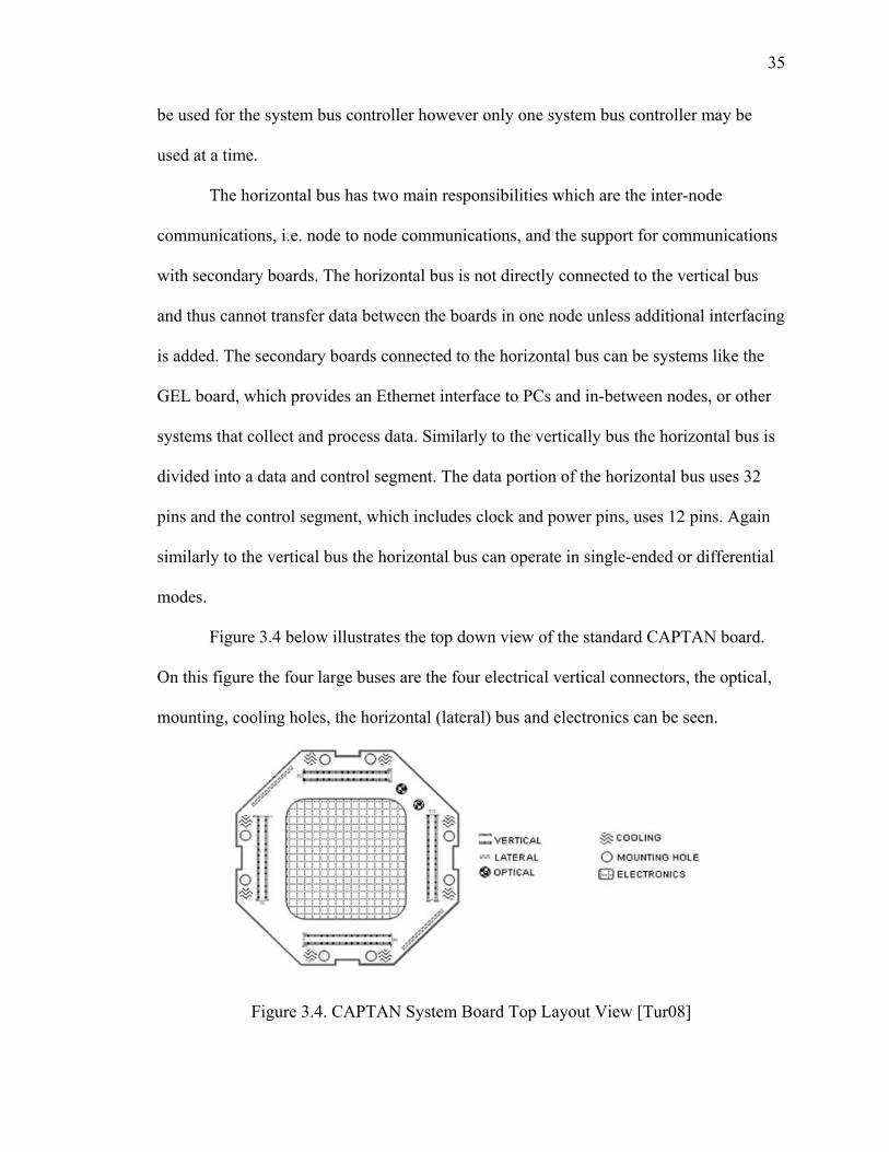
Figure 3.4 below illustrates the top down view of the standard CAPTAN board.
On this figure the four large buses are the four electrical vertical connectors, the optical,
mounting, cooling holes, the horizontal (lateral) bus and electronics can be seen.
Figure 3.4. CAPTAN System Board Top Layout View [Tur08]
36
As can be seen from figure 3.4 the four vertical bus connecters are symmetrical
around the center of the board. This was done so that the boards could be stacked in four
different orientations with respect to each other. This allows for more physical flexibility
of connecting external systems to the horizontal buses, since if they all lined up there
would be significant size restrictions on the external systems.
The hardware boards which in this work included the NPCB, GEL, and AMA
boards are also part of the node layer. The types of boards support by the CAPTAN
architecture can be divided into two categories: the primary boards and secondary. The
primary boards have three main features. They have direct access and are able to support
communications on the vertical bus, they cannot consume more than 12W of power, and
they must have the same physical characteristics such as size, shape, location of main
buses and location of mounting and cooling holes. Existing types of CAPTAN primary
boards are the Node Processing and Control Board (NPCB), the Data Conversion Board
(DCB), the Power Electronics Board (PEB), the Mass Memory Board (MMB), and the
Acoustic MEMS Array board (AMA).
The secondary boards connect with a CAPTAN node through the horizontal bus
and thus must support the horizontal bus interface. They may not have direct access to the
vertical bus. They don’t have any physical constrains besides having the ability to be
connected to the horizontal bus. The other constraints for the secondary boards are that
they must not use more than 3W of power. An existing secondary board is the Gigabit
Ethernet Link (GEL) board. As the CAPTAN architecture is designed to be expandable
either primary or secondary boards with specific functions can be designed as necessary
as long as they follow the requirements [Tur08, Tur10].
37
The Network Layer. This layer of the CAPTAN architecture supports node to node and
node to PC communications. On the node side the GEL board is responsible for this
communication. On the PC side a standard Gigabit Ethernet card is used. Routers and
switches for communication distribution are also supported. To increase speed for real
time applications the network layer uses the Universal Datagram Protocol (UDP). For the
transport layer the Internet Protocol (IP) is used. The number of nodes in a system is only
limited by the maximum transfer rate of the GEL router, and network card of the system.
A single node can support up to ten GEL boards allowing for a maximum of 10
simultaneous gigabit rate transfers to one node.
The Application Layer. This layer consists of the various PC software used for user
interface and PC to node interface. It was designed to be as modular, scalable and
expandable as possible. These features are needed since each CAPTAN node can be
made up of different types and number of boards. It is also likely that new types of boards
will be used in the future. The expendability is necessary since the number of nodes
needed is unknown. Lastly modularity is key since each system requires significant PC
processing power thus distributing the processing demand among multiple PCs or
multiple cores of a single PC is also desirable.
The application layer can be divided into the CAPTAN Global Master (GM), the
CAPTAN Controller (CC), and the CAPTAN Data Acquisition User Interface (DAUC).
The GM is the top most module of the application layer and must be lunched
before all others. Only one GM is required for a CAPTAN network and only one may be
present at a time. The function of the GM is to manage the other applications in the

38
network. This consists of adding and removing devices and applications to and from the
network, determining the master/slave relationship of various applications, prioritizing
controls, and maintaining information about the entire network.
The addition of devices and modules is performed by listening to a specific socket
for a TCP/IP connection requests. When a device such as CAPTAN node or module such
as DAUC requests a connection the GM performs handshaking to verify that the request
is correct and to determine who is requesting the connection. After this a new socket is
opened for future communications with the requesting device.
Maintaining the information about the network such as socket numbers, types of
devices, and types of applications allows the GM to control the communication between
all parties. Additionally the information about the network can be sent to a user if
requested.
The CC is the module that is responsible for managing and interfacing a
CAPTAN node with the rest of the system. Each CAPTAN node must have one and only
one CC module associated with it. The functions performed by the CC are the
transmission of commands from the GM to its CAPTAN node and the transmission of
data from its CAPTAN node to the GM and to a PC hard disk. Due to the high
throughput of the gigabit Ethernet connection the CAPTAN architecture requires some
PC memory and uses three threads. One thread is used to receive the gigabit rate data
from a CAPTAN node and store it into memory, another is used to receive commands
from the GM, and the last one is used to transmit the data stored in the memory to the
hard disk. This three thread configuration allows the software to take advantage of multi-
39
core PC which can run each thread separately thus preventing higher priority command
communications from being delayed by data transfers.
The DAUC is the main user interface through which a PC user communicates
with the CAPTAN nodes in the network. There can be multiple DAUC running on
multiple PC but only one of these may have control. This interface can be used to start
and stop data transmission to a PC from the various CAPTAN nodes in the network, to
view the data, and to configure any CC. Those DUACs that do not have control can only
view the data recorded by the nodes [Riv08, Tur10].
3.3 Node Processing and Control Board (NPCB)
The NPCB is the central board in the CAPTAN architecture with a large number
of functions. The two main functions of the board are the control and arbitration of the
buses and devices on all boards in a node through the use of the system control bus and
the programming of the various devices in a node through the use of the system SPI bus.
The board also performs the buffering and processing of information collected by the
various boards in a node. Lastly this board serves as the gateway for all information
collected in its node which is to be sent to other nodes in the network or a PC. As this
board is the central controller of a node at least one of these boards must be present in
every node, however more than one can also be used in which case only one of them has
master control of the system bus.
The central part of the NPCB is the VIRTEX-4 XC4CFX12 FPGA [Xil08]. This
is the unit that performs the processing for the functions provided by the NPCB. Another
important component of the NPCB is the 32MB E2PROM. This E2PROM is connected to
40
the FPGA and is used to store permanent configware which is required to run on the
FPGA when the node powers on. The configware stored in the E2PROM include the
System Bus Controller, and for the microphone array data acquisition system the
configware also includes the Acquisition Control Module, the Signal Processing Module,
and the Ethernet Communications Module.
As its name suggests the acquisition control configware is responsible for getting
data from the microphone array. This involves setting up the analog to digital converters
with parameters such as sampling rate and bit resolution, receiving data from the analog
to digital converters and formatting the data to be used by the signal processing
configware.
The signal processing block is the next part in the configware chain and receives
its data from the data acquisition module. The function of this module is to process the
data collected by the microphones. The simplest and default processing performed by this
configware is buffering and transmission of the microphone data in a binary format to the
Ethernet communication configware. This configware is the one that would typically be
modified by the user of the microphone acquisition system to perform some other
processing such as filtering, averaging or other more advance processing algorithms. It
should also be noted that since this processing is performed on the FPGA it significantly
improves performance possibly allowing real-time functionality.
The Ethernet communications configware is the last in the chain and receives its
data from the signal processing module. This module is responsible for formatting the
data received from the signal processing module to a UDP format and transmitting it to
the GEL board at a gigabit rate. This configware is also responsible for receiving data
41
through from the GEL board at a gigabit rate and converting it from a UDP format to the
format necessary by the other parts of the system.
Physically the NPCB follows the guidelines of a standard CAPTAN board. It has
four connecters for the electrical vertical bus, two horizontal buses, and an optical
vertical bus for laser communications. In the microphone array data acquisition system
the GEL board is connected the NPCB through one of the two horizontal buses. There is
also one JTAG connecter on the NPCB board for programming the FPGA and EPROM.
Another important issue with the NPCB boards is that the vertical bus clock speed
and in turn the maximum bus transfer rate is related to the number of boards present in a
node. The maximum vertical bus clock speed is achieved when only two boards are used.
This speed for a single-ended and differential mode of operation of the vertical bus is 200
MHz and 340 MHz, respectively. The largest number of boards that can be used without
introducing errors to the vertical bus on both modes of operations is seven. For seven
boards the maximum the speed for a single-ended and differential mode of operation of
the vertical bus is 33 MHz and 125MHz, respectively.
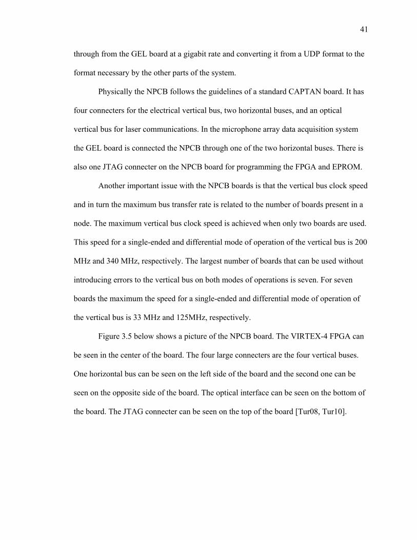
Figure 3.5 below shows a picture of the NPCB board. The VIRTEX-4 FPGA can
be seen in the center of the board. The four large connecters are the four vertical buses.
One horizontal bus can be seen on the left side of the board and the second one can be
seen on the opposite side of the board. The optical interface can be seen on the bottom of
the board. The JTAG connecter can be seen on the top of the board [Tur08, Tur10].

42
Figure 3.5. Top View Picture of the NPCB
3.4 Gigabit Ethernet Link (GEL) Board
The GEL board is the main network interface device for the CAPTAN nodes. It
can be used for node to node and node to PC communications. The main function of this
board is to format the information leaving a CAPTAN node into an Ethernet physical and
data link layer format and to convert received data from an Ethernet physical and data
link layer format. For the network layer the board uses the IP protocol and for the
transport layer the board uses the UDP protocol. The physical layer of the GEL board
uses the optic fiber 1000BASE-X standard [Tur08, Tur10].
The GEL board also supports the 10, 100, and 1000 Mbps speeds however the
default setting and the one used for the microphone array data acquisition system is 1000
Mbps. Due to the various layer framings being used the user data transfer rate is lower

43
than the overall transfer rate, this relationship and the overall maximum reliable transfer
rate are shown in the figure 3.6 below.
Figure 3.6. GEL Board Transfer Rate Graph [Tur08]
In this graph the top curve shows the data transferred and the bottom shows the
data lost. The vertical axis shows the rate at which useful user data is being transferred
and the horizontal axis shows the overall transfer rate which includes the framing
information. From this graph it can be seen that the maximum useful transfer rate is just
under 800 Mbps.
The GEL board is not a primary CAPTAN board and so it does not have to
conform to the same standard CAPTAN board physical requirements. As such this board
does not connect to a node through the vertical bus but only through the horizontal bus of
NPCB board. Additionally for the GEL board to work the NPCB board which it is
connected to must contain the Ethernet communications configware for the IP/UDP

44
portion of the communications. As each GEL board has its own IP and MAC address
there can be as many GEL boards in a node as there are NPCB boards. However due to
the high communication speeds of the gigabit Ethernet each GEL board consumes 1.25W
of power [Tur08, Tur10].
The GEL board can be seen in figure 3.7 below:
Figure 3.7. Top View Picture of the GEL Board
3.5 Acoustic MEMS Array (AMA)
The AMA board is a custom primary type CAPTAN board for acoustic and
ultrasound acquisition. This board uses 52 MEMS microphones for its sound and
ultrasound acquisition. In support of the 52 microphones the board also contains 52
amplifiers, 52 highpass filters, 52 analog to digital converters, and 52 of the circuits
connecting and regulating the microphone, amplifier, filter, and ADC configuration
[Tur10].
The 52 microphones are arranged in eight horizontal and eight vertical rows in an
octagonal shape matching the shape of the board. The inter microphone spacing is 10mm
center to center horizontally and vertically. The spacing of 10mm allows for spatial
45
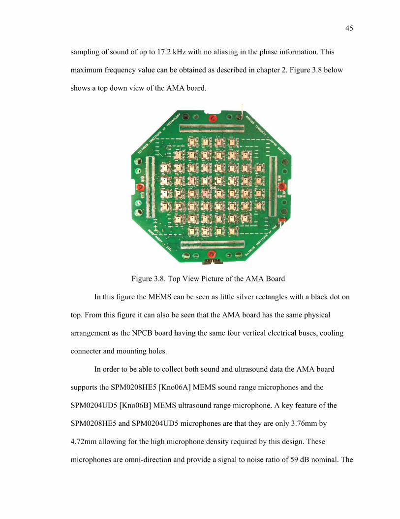
sampling of sound of up to 17.2 kHz with no aliasing in the phase information. This
maximum frequency value can be obtained as described in chapter 2. Figure 3.8 below
shows a top down view of the AMA board.
Figure 3.8. Top View Picture of the AMA Board
In this figure the MEMS can be seen as little silver rectangles with a black dot on
top. From this figure it can also be seen that the AMA board has the same physical
arrangement as the NPCB board having the same four vertical electrical buses, cooling
connecter and mounting holes.
In order to be able to collect both sound and ultrasound data the AMA board
supports the SPM0208HE5 [Kno06A] MEMS sound range microphones and the
SPM0204UD5 [Kno06B] MEMS ultrasound range microphone. A key feature of the
SPM0208HE5 and SPM0204UD5 microphones are that they are only 3.76mm by
4.72mm allowing for the high microphone density required by this design. These
microphones are omni-direction and provide a signal to noise ratio of 59 dB nominal. The
46
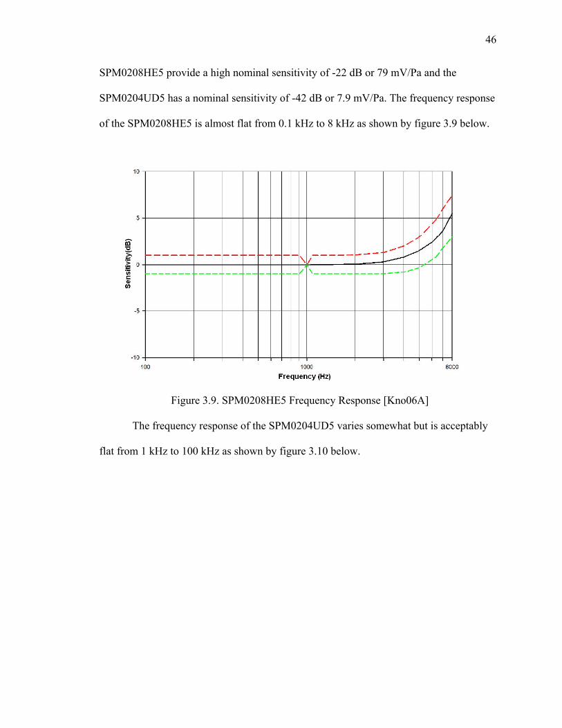
SPM0208HE5 provide a high nominal sensitivity of -22 dB or 79 mV/Pa and the
SPM0204UD5 has a nominal sensitivity of -42 dB or 7.9 mV/Pa. The frequency response
of the SPM0208HE5 is almost flat from 0.1 kHz to 8 kHz as shown by figure 3.9 below.
Figure 3.9. SPM0208HE5 Frequency Response [Kno06A]
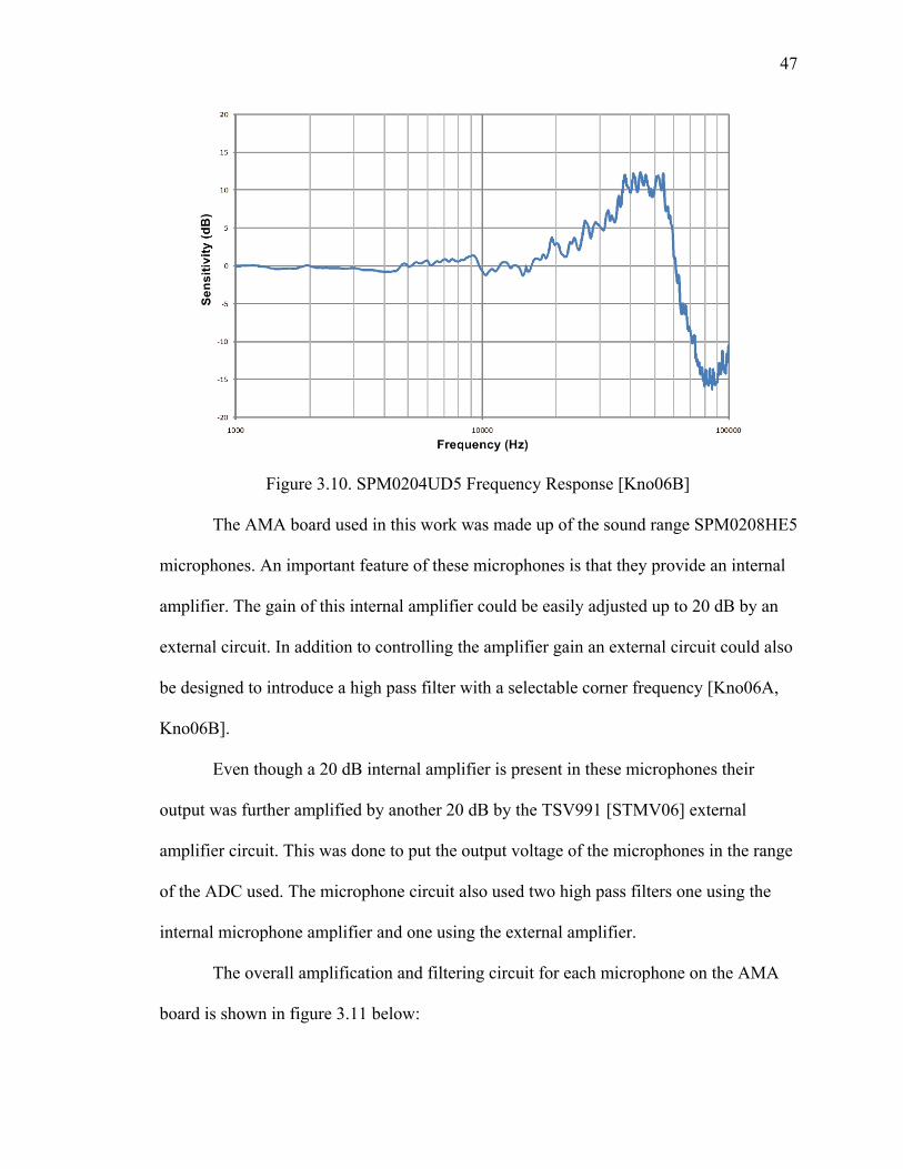
The frequency response of the SPM0204UD5 varies somewhat but is acceptably
flat from 1 kHz to 100 kHz as shown by figure 3.10 below.
47
Figure 3.10. SPM0204UD5 Frequency Response [Kno06B]
The AMA board used in this work was made up of the sound range SPM0208HE5
microphones. An important feature of these microphones is that they provide an internal
amplifier. The gain of this internal amplifier could be easily adjusted up to 20 dB by an
external circuit. In addition to controlling the amplifier gain an external circuit could also
be designed to introduce a high pass filter with a selectable corner frequency [Kno06A,
Kno06B].
Even though a 20 dB internal amplifier is present in these microphones their
output was further amplified by another 20 dB by the TSV991 [STMV06] external
amplifier circuit. This was done to put the output voltage of the microphones in the range
of the ADC used. The microphone circuit also used two high pass filters one using the
internal microphone amplifier and one using the external amplifier.
The overall amplification and filtering circuit for each microphone on the AMA
board is shown in figure 3.11 below:
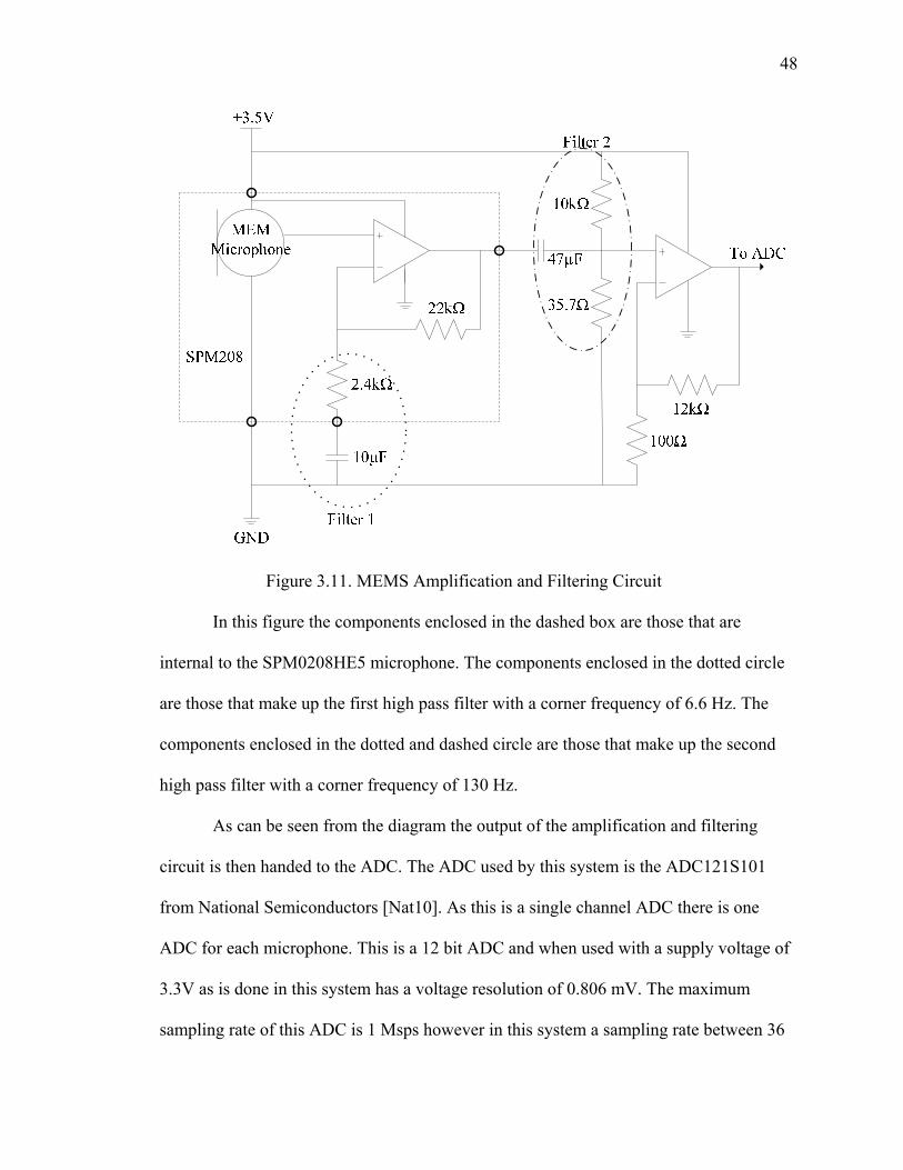
48
Figure 3.11. MEMS Amplification and Filtering Circuit
In this figure the components enclosed in the dashed box are those that are
internal to the SPM0208HE5 microphone. The components enclosed in the dotted circle
are those that make up the first high pass filter with a corner frequency of 6.6 Hz. The
components enclosed in the dotted and dashed circle are those that make up the second
high pass filter with a corner frequency of 130 Hz.
As can be seen from the diagram the output of the amplification and filtering
circuit is then handed to the ADC. The ADC used by this system is the ADC121S101
from National Semiconductors [Nat10]. As this is a single channel ADC there is one
ADC for each microphone. This is a 12 bit ADC and when used with a supply voltage of
3.3V as is done in this system has a voltage resolution of 0.806 mV. The maximum
sampling rate of this ADC is 1 Msps however in this system a sampling rate between 36
49
Ksps and 300 Ksps is used. When used at the higher sampling rate of 300 Ksps the output
of each ADC is 3.6 Mbps. The 52 microphones together generate 187 Mbps which is then
transferred through the four vertical bus connecters to the FPGA on the NPCB board.
From this it can be seen that the high speed of the four vertical buses and the gigabit
Ethernet rate connections are necessary for real-time applications of this system.
It is also important to mention that the AMA board used in this work is the AMA
II board which is the second generation of the CAPTAN acoustic array acquisition
boards. The AMA I board was used for testing and exploration purposes. The AMA II
board was then designed based on the observations obtained from the AMA I board. The
main differences between the two boards are that the AMA I board had 48 microphones,
the spacing between the microphones was 12 mm center to center, and the first board also
contained a central ultrasound transmitter for calibration and range testing [Tur08,
Tur10].
3.6 Restrictions and Requirements
This section summarizes the restrictions of the microphone array data acquisition
system. The main restriction of this system is that it must be connected to a computer to
work. Thus the system does not have its own interface and multiple nodes cannot connect
to one another without at least one central PC. However since the system has a central
FPGA it is possible to modify the system to have its own display, interface and node to
node networking capability.
An important point to mentions is that the PC software for this system uses high
speed transmission and requires a high speed processor and a significant amount of

50
RAM. Specifically the processor should have at least 2 cores at 2 GHz each and there
should be at least 2 Gigabytes of fast RAM. The hard-drive storage requirements for this
system are also high since as was shown earlier the system transmits approximately 187
Mbps to the PC. From this it can also be seen that even if a large hard drive is used either
the recorded data has to be used in real time and the earlier records must be erased to
make space for new ones or only a few seconds of data may be recorded.
Another restriction on the system is that the microphones are in fixed positions
allowing only one geometrical arrangement. One way to bypassed this limitation is to use
multiple systems in a network, however when only several microphones are required this
would be an inefficient use of resources. Another way to bypass this problem is to
disconnect the microphones from the board place them in required remote locations and
then run wiring to the array board.
As stated earlier due to the inter microphone distance the limitation on the
frequency of which the phase information can be used without aliasing is 17.2 kHz. The
overall limit on the maximum frequency of a signal this system can sampling is 150 kHz
since the maximum sampling of the ADC is 300 Ksps and by the Nyquist–Shannon
theorem the maximum frequency is half of the maximum sampling rate. Since this system
works with sound and ultrasound this is not a large problem as the sound range is
significantly lower and most ultrasound applications can also be done at significantly
lower frequencies.
51
3.7 Advantages
The microphone array data acquisition system and the CAPTAN architecture are
very versatile, computationally powerful, possess high speed communications, and are
designed with a broad range of applications in mind [Tur08, Tur10]. Due to these features
this system has a large number of advantages over other data acquisition systems.
One significant advantage of this system is its utility for prototyping. Specifically
various algorithms can be tested using a computer with high level programming, such as
MATLAB, as opposed to immediately working with a hardware description language.
Further due to the gigabit rate of communications algorithm testing can be extend to real-
time as the transfer of the data to the PC does not form a bottleneck.
Another important feature of the system is the large processing power provided by
the embedded Virtex-4 FPGA. This power can be seen from the system’s ability to
simultaneously process the data coming in from the 52 ADC of which each is generating
3.6Mbps. In addition to the basic processing being performed on this data the system also
has the capability of running more advanced algorithms as required. As the Virtex-4
FPGA is used there is also an option to use the hardcore power PC processer for
algorithm implementation [Xil08]. Thus this system allows several approaches for
algorithm implementation ranging from the easy to implement but slow performing
computer based implementation to the more difficult to implement but faster performing
hardware description language implementation.
The large number of input channels of the array is also a key feature. Standard
data acquisition systems such as oscilloscopes only use two and less frequently four
channels [Agi10B]. Having access to only two or four channels poses several problems.
52
One is that some applications may simply need more channels of information to function.
An example of this is triangulation which requires at least three channels for three sensor
inputs, other applications may be distributed sensing or security which may have to
collect data from dozens of places and then combine or compare it for an overall picture.
An additional issue with using a smaller number of sensors is that it may increase
the computational complexity of the algorithms used to get a certain result from the
collected data, that is, it may be easier to extract certain information when a larger
number of sensors are used. An example of this is 3D source localization, where it is
possible to get the position of a sound source using three microphones, however this
would involve solving three 3D conic equations, however if five sensors are used only
four 2D triangle equations have to be solved.
Another advantage of using a large number of sensors is that it allows for an
increase in the confidence of your results and for a reduction of errors due to various
interferences. For example suppose that the same data is being collected by twelve
sensors and one or two are giving different readings than the other ten sensors. Since
twelve sensors are being used it is possible to discard the data from the two mismatching
sensors and still be confident of the result obtained from the other ten sensors.
An advantage of the CAPTAN architecture as a whole is that it was designed to
be expandable and scalable. As stated earlier each node can have any mixture of boards
as required by the application. Physically the octagonal shape of the primary boards
allows for tiling with a corner slot for running cables or wires. Lastly the networking
capabilities of the architecture allow a large number of systems to work together in either
a distributed or tiled configuration.
53
CHAPTER 4
GENERAL DATA ACQUISITION AND GENERATION
4.1 Oscilloscope Based Data Acquisition
As a comparison to the custom designed microphone array data acquisition
system, the capabilities of the Agilent MSO6032A standard mixed signal oscilloscope are
explored. Specifically the various techniques of capturing and transmitting data to a PC
are presented. Several different styles of programmatic control and data acquisition are
also investigated. Lastly various interfaces and networking capabilities of the
oscilloscope are examined.
The simplest and quickest way to obtain data from the MSO6032A oscilloscope is
through the use of a USB external storage device. This simply involves connecting the
USB storage device to the scope and using the front panel to configure the scope to save
to the device under a specific name and in a specific format. The possible formats in
which the data can be saved are a graphical image of the display and an XY coordinate
data set file. Each one of the formats can be of several types such as BMP, PNG, ASCII-
XY, BIN-XY, and others. The ASCI-XY and BIN-XY formats can then be loaded to a
PC from the USB storage device. Programs such as Excel and Matlab can then use these
files for algorithm application and graphical display.
In addition to saving the waveform data the overall configuration, such as
triggering, time scale, and voltage scale of the oscilloscope could also be saved and later
recalled to avoid readjusting the settings of the oscilloscope every time it is turned on and
off. The trace of a waveform can also be saved and recalled. This somewhat mitigates the
limitation of having only two or four channels since many traces can be saved and then
54
recalled for comparison. Another set of information that can be saved is the measurement
information of the waveform on the oscilloscope. These measurements can be things like
voltage, frequency, duty cycle and many others. The limitation on this type of acquisition
is that it involves several transfers one from the oscilloscope to a USB storage device,
one from the storage device to a PC, and one from a file on the PC to a program like
Matlab. [Agi10B].
The second option for transferring data from the oscilloscope to a PC is to use the
Agilent IntuiLink Data Capture software. This is a Graphic User Interface (GUI) software
which features all the capabilities described for the USB external storage device but with
several advantages. First it directly connects the PC to the scope removing the need for an
intermediate storage. This connection can be made using either a USB port and LAN
interface, or GPIB interface. The second advantage is that it allows for a convenient PC
interface to be used, otherwise the two techniques are the same [Agi09A].
The oscilloscope can also be accessed remotely through the internet using the
oscilloscope’s built in web server. The functions of this interface can be divided into four
groups. First this interface allows you to view, and in some cases modify, information
about the oscilloscope like its model number, serial number, host name, IP address, VISA
(address), installed options, firmware versions, calibration status, network configuration
and status information. Second this interface allows you to get screen images of the
oscilloscope’s display. This remote interface also allows the oscilloscope to be
programmatically controlled using the oscilloscope’s Standard Commands for
Programmable Instruments (SCPI). The details of how SCPI programming works will be
discussed next. Lastly the web server interface allows the users to see and control the

55
oscilloscope through a GUI of the front panel and screen of the oscilloscope. This is a
Java based GUI which is a virtual equivalent of the physical oscilloscope, i.e. the virtual
GUI has a screen display which looks like the real physical oscilloscope display and it
also has the functionality of all the physical front panel buttons and knobs [Agi10B]. The
limitation on this interface is that only the image can be transferred to a remote user and
not the actual XY data points. This may be modified later as, in general, it is possible to
read the data points using the SCPI commands however there needs to be a way to save
this information into a file on the remote PC [Agi10A].
The most complex method but also the one that gives the most control for
interfacing with the oscilloscope is through the use of its programming capabilities. This
method allows the user to both control the oscilloscope and acquire data from the
oscilloscope. In general programming of the oscilloscope can be divided into two groups,
direct programming and driver based programming. Each of these approaches can be
performed through the use of several different high level programming languages such as
C, C++, Visual Basic, LabVIEW, Matlab and many others, the high level programming
language used in this work was Matlab.
Direct programming of the oscilloscope is performed by using the instrument
specific SCPI instructions or commands. All the functionality of the instrument, in this
case an oscilloscope, can be accessed through the use of these commands. However even
though these commands are somewhat standardized they still differ from oscilloscope to
oscilloscope as each one has different capabilities and accordingly has a different design
and different functionality [IVI09]. The commands for this approach are at a low level
thus several commands might be required to perform one conceptual operation such as

56
getting the time scale or reading in a waveform. Additionally programming at this level
requires basic knowledge of the oscilloscope’s architecture as reading and writing to
various status registers is involved at this level of programming. These issues make
directly programming the oscilloscope somewhat difficult.
It is however not extremely difficult to program the oscilloscope at this level as
the commands are somewhat standardized and are organized in to conceptually easily
manageable groups. Also most of the commands correspond to oscilloscope settings and
features and thus can be intuitively understood by anyone who uses the standard front
panel interface of the oscilloscope. As stated earlier this approach is the most powerful as
it gives access to all the features of the oscilloscope. In addition to this using the SCPI
commands and a high level programming language, a variety of scripts and programs can
be written for the oscilloscope to perform more complex and more controlled data
acquisition. These programs can then be run as necessary by people that are not familiar
with SCPI command programming.
To send the SCPI commands to the oscilloscope Matlab or another high level
programming language needs to be used. This consists of establishing an interface with
the oscilloscope and then sending commends or queries and receiving responses. Some of
the types of interfaces that can be used are VISA, USB, Serial, GPIB, TCP/IP and UDP.
This allows both local and remote control and data acquisition using the oscilloscope.
The need to use a high level language on top of the SCPI commands also adds some
complexity as both the high level language commands and syntax and the SCPI
command and syntax need to be learned. However there are relatively few high level
commands used for this purpose [Mat10].
57
The second programming based approach is to use drivers. Drivers are basically a
mapping of SCPI commands to higher level functions and oscilloscope properties. The
types of driver can be broadly divided into two groups: instrument specific and
instrument type drivers. Instrument specific drivers are designed for a particular
instrument such as a specific oscilloscope and thus offer access to all of the instrument’s
functionality. The advantage of using an instrument specific driver as compared to using
SCPI command programming is that instrument specific drivers have easy to understand
high level functions or methods instead of a combination of low level commands. For
example functions may be as simple as run() to run the oscilloscope or channel1.range(2)
to set the voltage range on channel 1 to 2 volts.
However the high level functions used by one instrument specific driver may not
be the same as that of another. For example two different instrument specific drivers for
two different oscilloscopes may use the following two function to read the voltage scale:
agilent.channel1.range() versus teck.chn1.rng(). Additionally different high level
functions must exist for different instrument specific drivers since each instrument may
have different features such as one being able to calculate cross correlation between two
channels and another being able to calculate the Fast Fourier Transform of a channel
[IVI09].
The second category of drivers is the instrument type driver. Instrument type
drivers address the limitation of the non-interchangeability of the instrument specific
drivers. These drivers also have the advantage of using easy to understand high level
functions or methods instead of a combination of low level SCPI commands. However
the high level functions for instrument type drivers are always the same for a specific
58
instrument type like an oscilloscope. This is done by having high level functions only for
the functionality that is common to all instruments of a specific type. Some drivers like
IVI drivers further divide this into base functionality functions and extension
functionality functions. Here the base functionality is the absolute least common
denominator functionality for an instrument type and has to be supported for all its
instrument type drivers using the same functions. The extension functionality is pretty
common for an instrument type so it does not have to be supported but if it is, it also uses
the same high level functions [IVI09].
Using instrument type drivers for ease of interchangeability of course comes at
the price of giving up a certain level of control over the instrument and losing the ability
to use all the instrument functionality and features. However the main advantage of using
interchangeable drivers is that when a program is written using the functions of an
interchangeable driver it can be run for any instrument of that type. The only thing that
needs to be changed is the instrument driver that will perform the mapping from the
instrument specific SCPI commands to the common high level functions.
Using driver is similar to using SCPI commands in that both use a high level
programming language such as Matlab or others as an interface. For drivers this consists
of loading the driver and establishing an interface with the oscilloscope. There is a
number of ways in which this can be done depending on the driver type and on the high
level language used. For example in Matlab this can be done through the command line
or through a GUI and for IVI drivers either an instance of the driver or a configuration
store and a session factory can be used [IVI09, Mat10]. The same type of interfaces are
available for both SCPI command programming and driver programming, specifically the

59
types of interfaces that can be used are VISA, USB, Serial, GPIB, TCP/IP and UDP.
Thus drivers based programming control and data acquisition can also be done remotely
or locally [Mat10].
4.2 Arbitrary Waveform Based Data Generation
For the sound and ultrasound experiments performed in this work a variety of
different waveforms were needed. Generation of these waveforms was accomplished
through the use of the Agilent 33220A function/arbitrary waveform generator [Agi07]. A
typical function generator can easily generate common waveforms such as a sin, square,
and ramp however sometimes these basic waveforms are not sufficient. For example for
basic ultrasound experiments a pulse or a train of pulses waveform is necessary.
Although this is not a basic waveform some function generators, such as the Agilent
33220A, have a build in interface to allow these types of signals to be generated.
However sometimes even more complex waveforms such as several different length
pulse trains, random shape waves, combinational waves, prerecorded real signals or
prerecorded and modified real signals are needed. These types of signals can only be
obtained by using an arbitrary waveform generator such as the Agilent 33220A.
There are three ways in which arbitrary waveforms can be generated using the
Agilent 33220A [Agi09C]. The simples but least effective way to generate arbitrary
waveforms is through the use of the front panel interface of the arbitrary waveform
generator. This involves inputting the waveform point by point specifying the amplitude
and interval between successive points. This waveform can then be saved to the
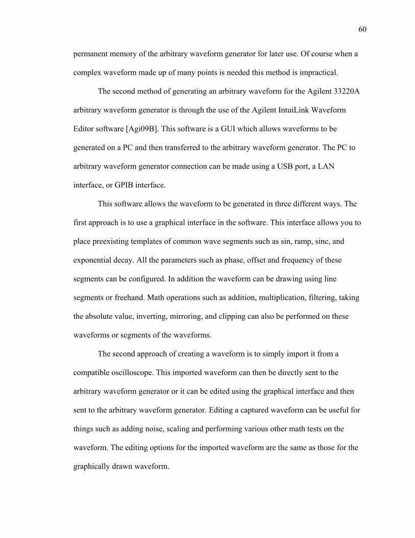
60
permanent memory of the arbitrary waveform generator for later use. Of course when a
complex waveform made up of many points is needed this method is impractical.
The second method of generating an arbitrary waveform for the Agilent 33220A
arbitrary waveform generator is through the use of the Agilent IntuiLink Waveform
Editor software [Agi09B]. This software is a GUI which allows waveforms to be
generated on a PC and then transferred to the arbitrary waveform generator. The PC to
arbitrary waveform generator connection can be made using a USB port, a LAN
interface, or GPIB interface.
This software allows the waveform to be generated in three different ways. The
first approach is to use a graphical interface in the software. This interface allows you to
place preexisting templates of common wave segments such as sin, ramp, sinc, and
exponential decay. All the parameters such as phase, offset and frequency of these
segments can be configured. In addition the waveform can be drawing using line
segments or freehand. Math operations such as addition, multiplication, filtering, taking
the absolute value, inverting, mirroring, and clipping can also be performed on these
waveforms or segments of the waveforms.
The second approach of creating a waveform is to simply import it from a
compatible oscilloscope. This imported waveform can then be directly sent to the
arbitrary waveform generator or it can be edited using the graphical interface and then
sent to the arbitrary waveform generator. Editing a captured waveform can be useful for
things such as adding noise, scaling and performing various other math tests on the
waveform. The editing options for the imported waveform are the same as those for the
graphically drawn waveform.
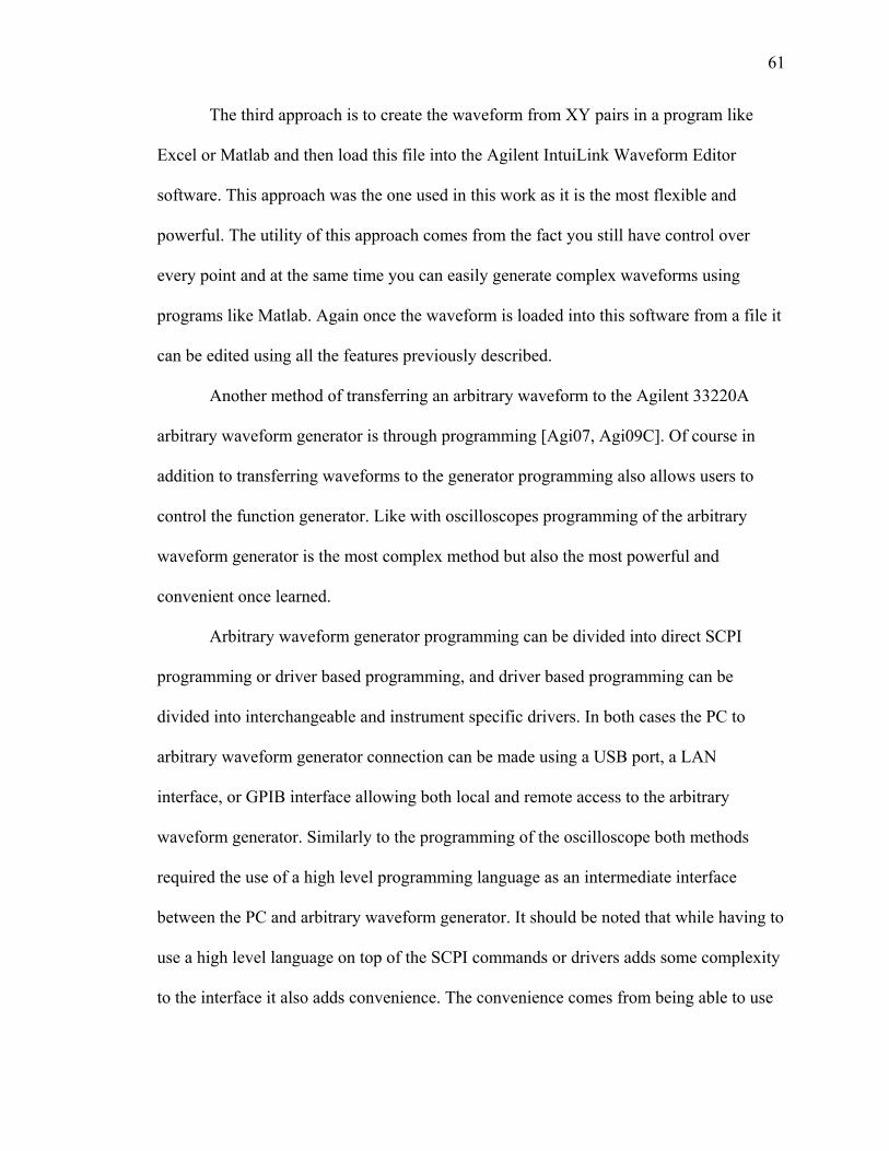
61
The third approach is to create the waveform from XY pairs in a program like
Excel or Matlab and then load this file into the Agilent IntuiLink Waveform Editor
software. This approach was the one used in this work as it is the most flexible and
powerful. The utility of this approach comes from the fact you still have control over
every point and at the same time you can easily generate complex waveforms using
programs like Matlab. Again once the waveform is loaded into this software from a file it
can be edited using all the features previously described.
Another method of transferring an arbitrary waveform to the Agilent 33220A
arbitrary waveform generator is through programming [Agi07, Agi09C]. Of course in
addition to transferring waveforms to the generator programming also allows users to
control the function generator. Like with oscilloscopes programming of the arbitrary
waveform generator is the most complex method but also the most powerful and
convenient once learned.
Arbitrary waveform generator programming can be divided into direct SCPI
programming or driver based programming, and driver based programming can be
divided into interchangeable and instrument specific drivers. In both cases the PC to
arbitrary waveform generator connection can be made using a USB port, a LAN
interface, or GPIB interface allowing both local and remote access to the arbitrary
waveform generator. Similarly to the programming of the oscilloscope both methods
required the use of a high level programming language as an intermediate interface
between the PC and arbitrary waveform generator. It should be noted that while having to
use a high level language on top of the SCPI commands or drivers adds some complexity
to the interface it also adds convenience. The convenience comes from being able to use
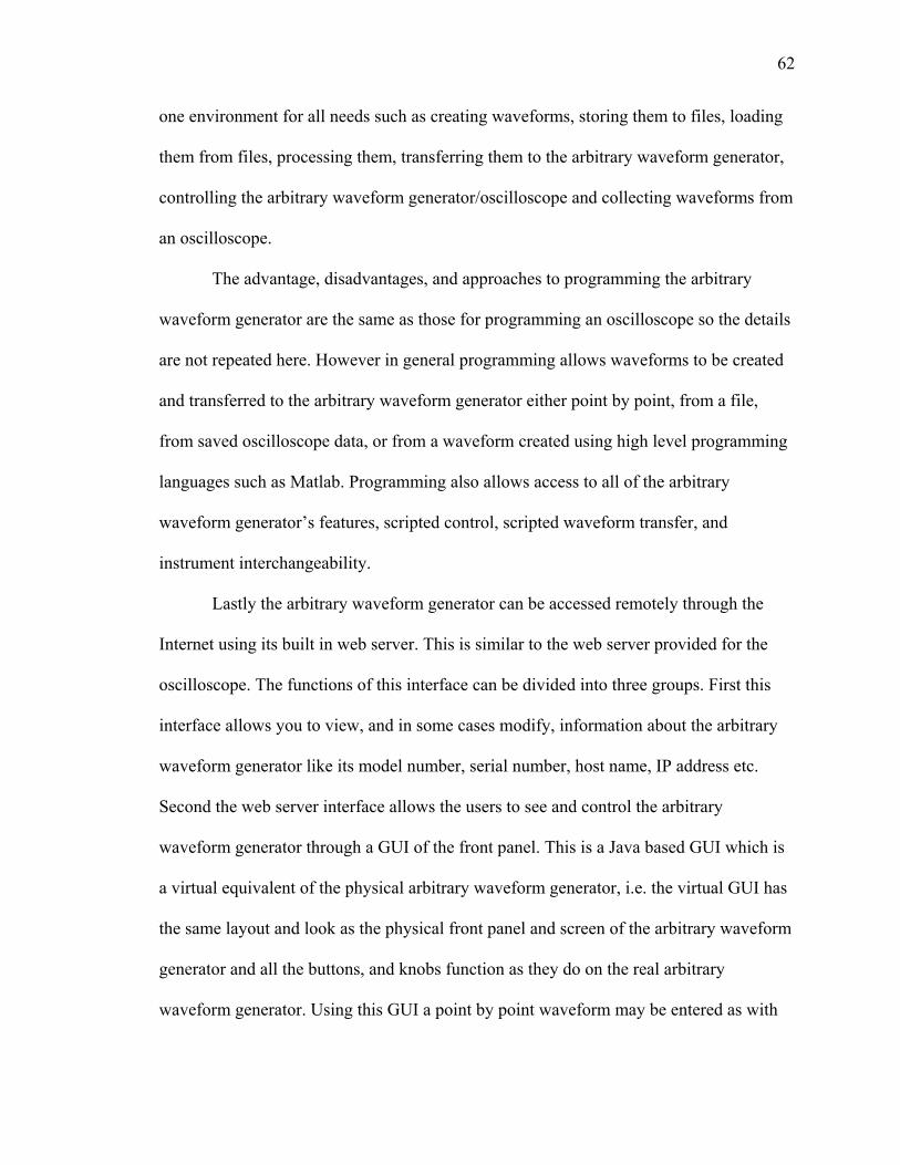
62
one environment for all needs such as creating waveforms, storing them to files, loading
them from files, processing them, transferring them to the arbitrary waveform generator,
controlling the arbitrary waveform generator/oscilloscope and collecting waveforms from
an oscilloscope.
The advantage, disadvantages, and approaches to programming the arbitrary
waveform generator are the same as those for programming an oscilloscope so the details
are not repeated here. However in general programming allows waveforms to be created
and transferred to the arbitrary waveform generator either point by point, from a file,
from saved oscilloscope data, or from a waveform created using high level programming
languages such as Matlab. Programming also allows access to all of the arbitrary
waveform generator’s features, scripted control, scripted waveform transfer, and
instrument interchangeability.
Lastly the arbitrary waveform generator can be accessed remotely through the
Internet using its built in web server. This is similar to the web server provided for the
oscilloscope. The functions of this interface can be divided into three groups. First this
interface allows you to view, and in some cases modify, information about the arbitrary
waveform generator like its model number, serial number, host name, IP address etc.
Second the web server interface allows the users to see and control the arbitrary
waveform generator through a GUI of the front panel. This is a Java based GUI which is
a virtual equivalent of the physical arbitrary waveform generator, i.e. the virtual GUI has
the same layout and look as the physical front panel and screen of the arbitrary waveform
generator and all the buttons, and knobs function as they do on the real arbitrary
waveform generator. Using this GUI a point by point waveform may be entered as with

63
the real arbitrary waveform generator. The last function of the web server interface is to
allow SCPI programming of the arbitrary waveform generator. Using the SCPI
commands of this interface also allows waveforms to be entered into the arbitrary
waveform generator.

64
CHAPTER 5
ACOUSTIC CHAMBER, MEASUREMENT MOUNT AND SENSOR ARRAY TEST STAND
5.1 Acoustic Chamber
To create a controlled environment for acoustic experimentation an acoustic
chamber was designed and built. The key features of the chamber are its ability to isolate
the experiment inside the chamber from outside noise and to absorb sound inside the
chamber to prevent reverberation and reflections. It should be noted that while the noise
from outside of the chamber could be either reflected back outside or absorbed by the
chamber, sound inside the chamber has to be absorbed by the surfaces of the chamber to
prevent reflections. The material used for sound absorption was foam, however the
chamber was designed in such a way that other materials with different acoustic
absorption properties could be attached to the same chamber structure. For ease of
portability the chamber is also disassemble into small and light pieces. Since the size and
setup of the experiments which are to be performed are not known beforehand the
chamber is designed to be modular allowing its size to be adjusted as necessary for a
wide variety of experiments. Lastly the chamber is designed to be easily opened and
closed allowing the experimental setup to be quickly and effortlessly modified as
necessary.
Figures 5.1 and 5.2 below shows the outside view of the assembled acoustic
chamber from the top and side, respectively. Figures 5.3 and 5.4 below show the inside
view of the assembled acoustic chamber from the top and side, respectively.
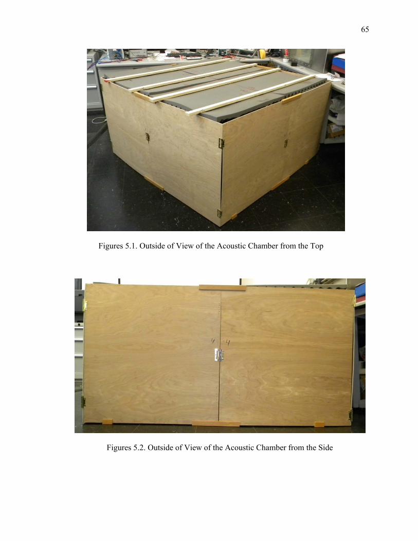
65
Figures 5.1. Outside of View of the Acoustic Chamber from the Top
Figures 5.2. Outside of View of the Acoustic Chamber from the Side
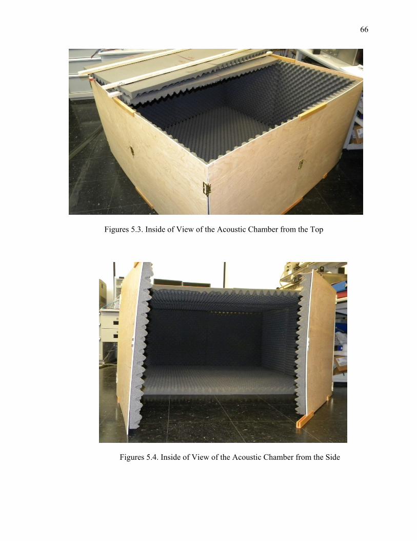
66
Figures 5.3. Inside of View of the Acoustic Chamber from the Top
Figures 5.4. Inside of View of the Acoustic Chamber from the Side
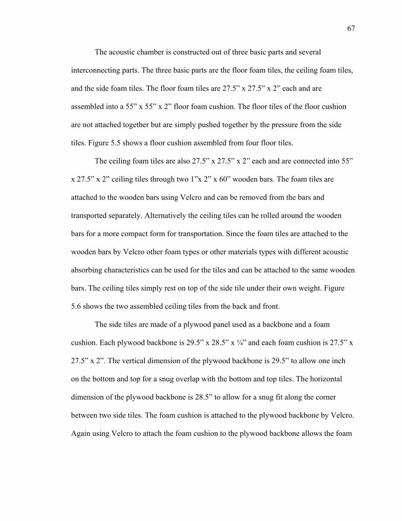
67
The acoustic chamber is constructed out of three basic parts and several
interconnecting parts. The three basic parts are the floor foam tiles, the ceiling foam tiles,
and the side foam tiles. The floor foam tiles are 27.5” x 27.5” x 2” each and are
assembled into a 55” x 55” x 2” floor foam cushion. The floor tiles of the floor cushion
are not attached together but are simply pushed together by the pressure from the side
tiles. Figure 5.5 shows a floor cushion assembled from four floor tiles.
The ceiling foam tiles are also 27.5” x 27.5” x 2” each and are connected into 55”
x 27.5” x 2” ceiling tiles through two 1”x 2” x 60” wooden bars. The foam tiles are
attached to the wooden bars using Velcro and can be removed from the bars and
transported separately. Alternatively the ceiling tiles can be rolled around the wooden
bars for a more compact form for transportation. Since the foam tiles are attached to the
wooden bars by Velcro other foam types or other materials types with different acoustic
absorbing characteristics can be used for the tiles and can be attached to the same wooden
bars. The ceiling tiles simply rest on top of the side tile under their own weight. Figure
5.6 shows the two assembled ceiling tiles from the back and front.
The side tiles are made of a plywood panel used as a backbone and a foam
cushion. Each plywood backbone is 29.5” x 28.5” x ¼” and each foam cushion is 27.5” x
27.5” x 2”. The vertical dimension of the plywood backbone is 29.5” to allow one inch
on the bottom and top for a snug overlap with the bottom and top tiles. The horizontal
dimension of the plywood backbone is 28.5” to allow for a snug fit along the corner
between two side tiles. The foam cushion is attached to the plywood backbone by Velcro.
Again using Velcro to attach the foam cushion to the plywood backbone allows the foam
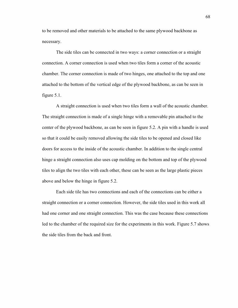
68
to be removed and other materials to be attached to the same plywood backbone as
necessary.
The side tiles can be connected in two ways: a corner connection or a straight
connection. A corner connection is used when two tiles form a corner of the acoustic
chamber. The corner connection is made of two hinges, one attached to the top and one
attached to the bottom of the vertical edge of the plywood backbone, as can be seen in
figure 5.1.
A straight connection is used when two tiles form a wall of the acoustic chamber.
The straight connection is made of a single hinge with a removable pin attached to the
center of the plywood backbone, as can be seen in figure 5.2. A pin with a handle is used
so that it could be easily removed allowing the side tiles to be opened and closed like
doors for access to the inside of the acoustic chamber. In addition to the single central
hinge a straight connection also uses cap molding on the bottom and top of the plywood
tiles to align the two tiles with each other, these can be seen as the large plastic pieces
above and below the hinge in figure 5.2.
Each side tile has two connections and each of the connections can be either a
straight connection or a corner connection. However, the side tiles used in this work all
had one corner and one straight connection. This was the case because these connections
led to the chamber of the required size for the experiments in this work. Figure 5.7 shows
the side tiles from the back and front.
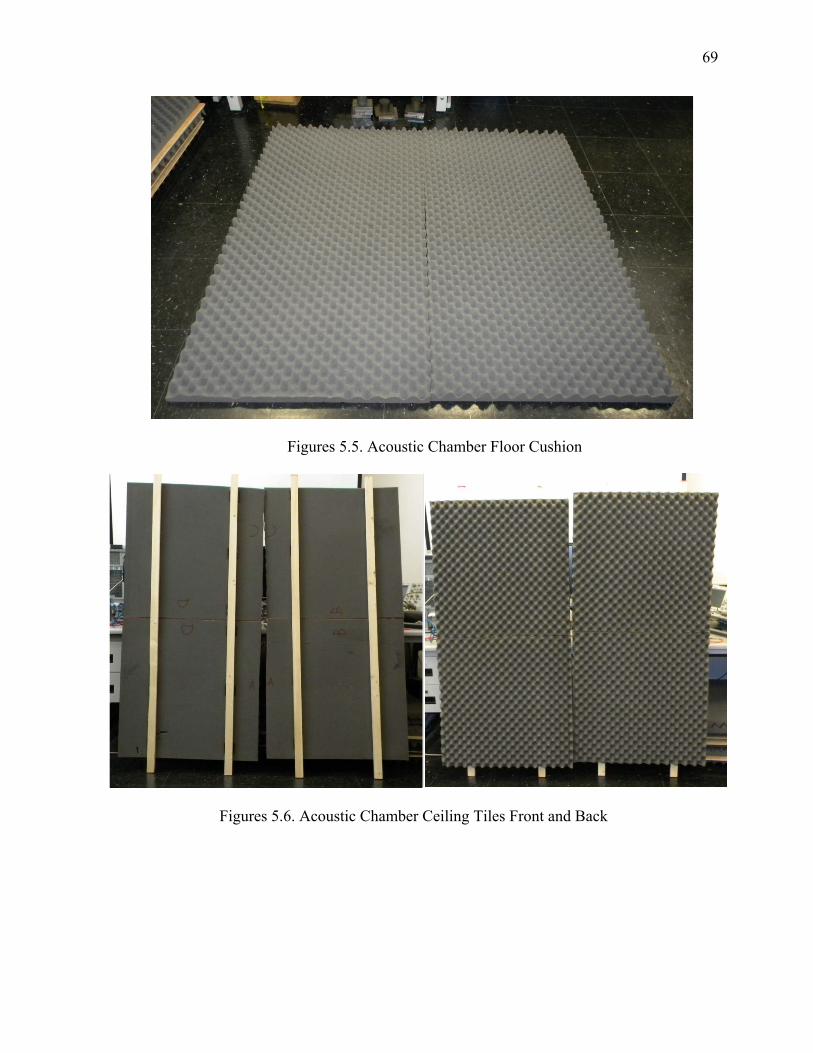
69
Figures 5.5. Acoustic Chamber Floor Cushion
Figures 5.6. Acoustic Chamber Ceiling Tiles Front and Back

70
Figures 5.7. Acoustic Chamber Side Tiles Front and Back
The size of the chamber can be easily changed although its shape must remain
rectangular. The size of the floor cushion can be simply changed by increasing or
decreasing the number of floor tiles used. The size of the ceiling can be changed in both
width and length. To increase the length of the ceiling more of the same ceiling tiles can
be used and can again rest on the side tiles. To increase the width of the ceiling, wooden
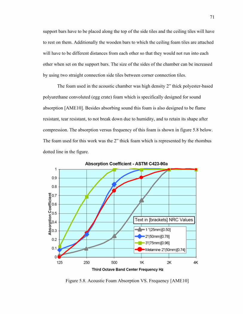
71
support bars have to be placed along the top of the side tiles and the ceiling tiles will have
to rest on them. Additionally the wooden bars to which the ceiling foam tiles are attached
will have to be different distances from each other so that they would not run into each
other when set on the support bars. The size of the sides of the chamber can be increased
by using two straight connection side tiles between corner connection tiles.
The foam used in the acoustic chamber was high density 2” thick polyester-based
polyurethane convoluted (egg crate) foam which is specifically designed for sound
absorption [AME10]. Besides absorbing sound this foam is also designed to be flame
resistant, tear resistant, to not break down due to humidity, and to retain its shape after
compression. The absorption versus frequency of this foam is shown in figure 5.8 below.
The foam used for this work was the 2” thick foam which is represented by the rhombus
dotted line in the figure.
Figure 5.8. Acoustic Foam Absorption VS. Frequency [AME10]

72
5.2 Measurement Mount
To accurately measure the angle and distance for sound source localization
experiments a special microphone mount was designed. The mount was based on the
Panavise 333 circuit board vise [PAN10]. This vise was used as it can be rotated around
all three axes and the distance and orientation of the vise arms, which hold the
microphones, can be easily adjusted. This vise is also based on a heavy yet small steel
plate for easy placement.
The main modification to the vise was the addition of a laser based angle
indicator. The indicator was constructed out of steel strips, a protractor, a laser pointer
and cable ties. The steel strip was bent around the central bar of the vise in such a way as
to be perpendicular to it. The strip was then attached to the bar using a screw. A
protractor and a second steel strip with a laser pointer attached to it using cable ties, was
then screwed on to the first steel strip.
Angle measurements are performed by rotating the second steel strip with the
laser pointer along the protractor to the desired angle, any object that is then aligned with
the dot created by the laser pointer is at the desired angle. In addition, to accurately
measure distances a rope with distance markers was tied around the steel strip. Figures
5.9 and 5.10 below show the front and side views of the measurement mount. It should
also be noted that while the figures show two microphones attached to the vise through
foam, these pieces could be removed and other systems such as the microphone array
data acquisition system could be mounted using the vise clamp arms.
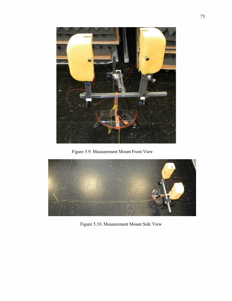
73
Figure 5.9. Measurement Mount Front View
Figure 5.10. Measurement Mount Side View
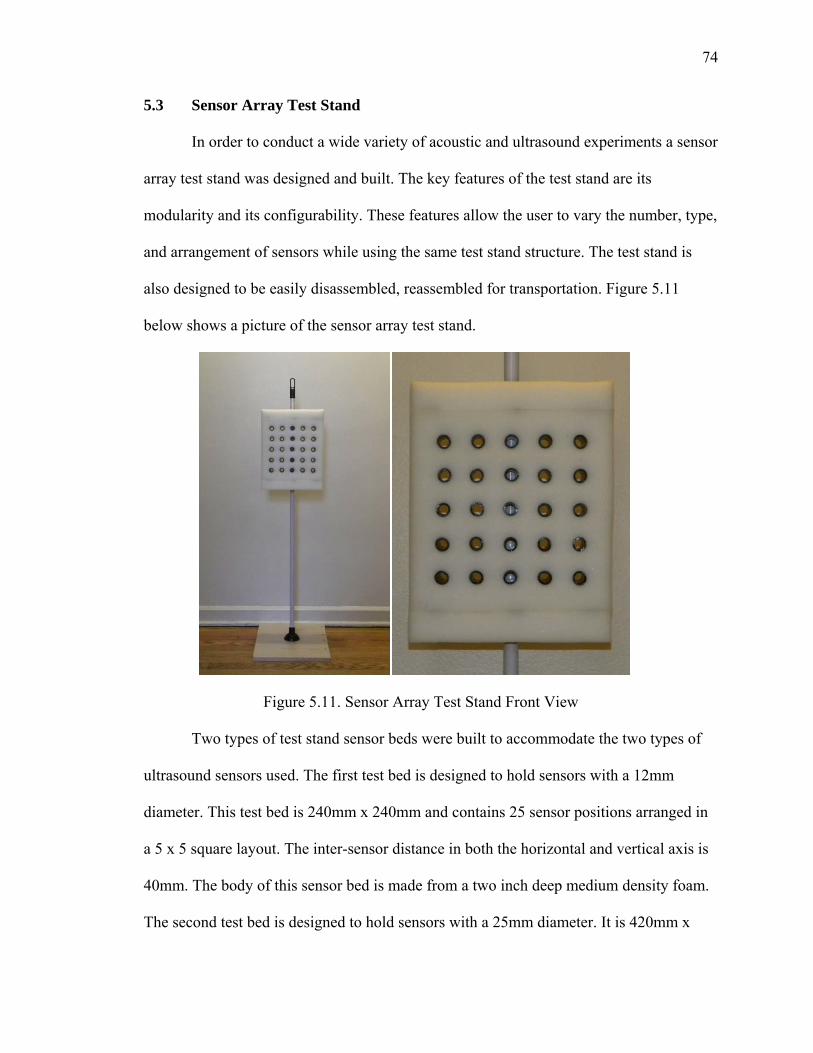
74
5.3 Sensor Array Test Stand
In order to conduct a wide variety of acoustic and ultrasound experiments a sensor
array test stand was designed and built. The key features of the test stand are its
modularity and its configurability. These features allow the user to vary the number, type,
and arrangement of sensors while using the same test stand structure. The test stand is
also designed to be easily disassembled, reassembled for transportation. Figure 5.11
below shows a picture of the sensor array test stand.
Figure 5.11. Sensor Array Test Stand Front View
Two types of test stand sensor beds were built to accommodate the two types of
ultrasound sensors used. The first test bed is designed to hold sensors with a 12mm
diameter. This test bed is 240mm x 240mm and contains 25 sensor positions arranged in
a 5 x 5 square layout. The inter-sensor distance in both the horizontal and vertical axis is
40mm. The body of this sensor bed is made from a two inch deep medium density foam.
The second test bed is designed to hold sensors with a 25mm diameter. It is 420mm x
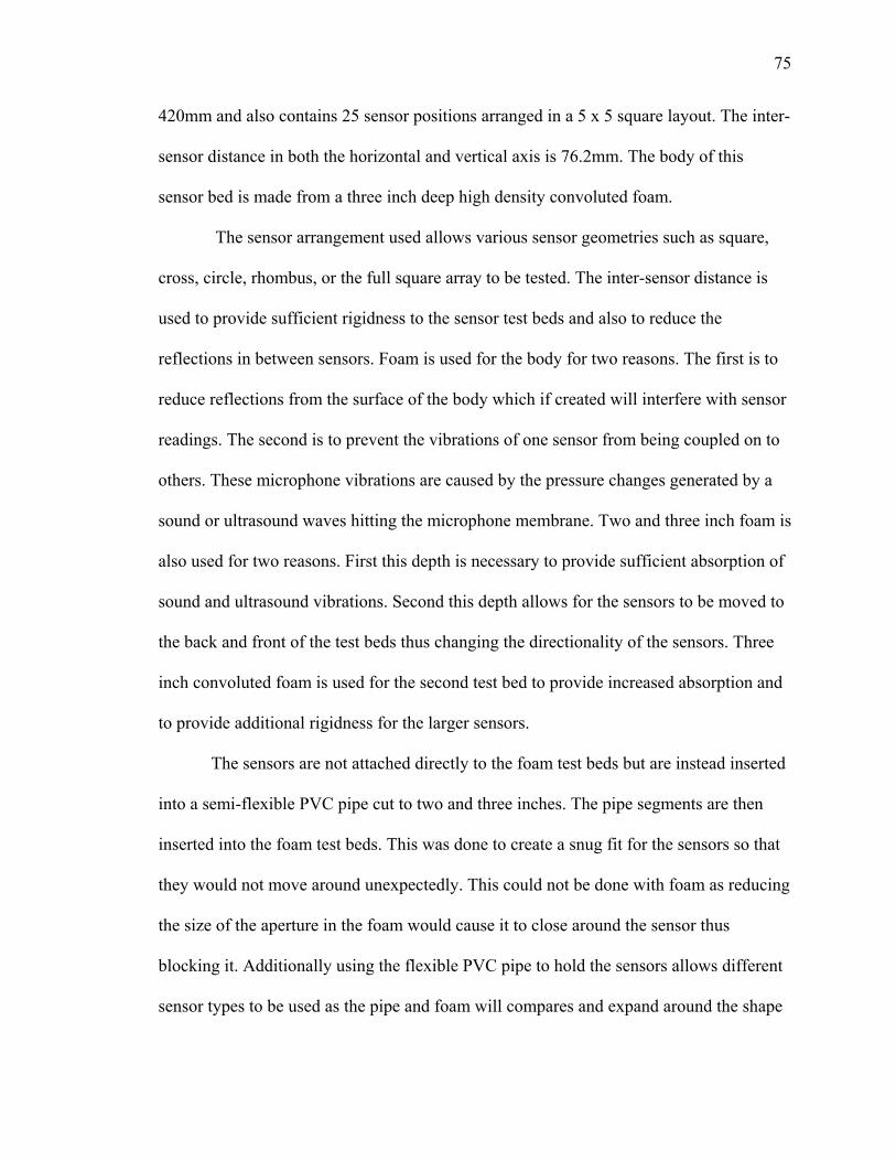
75
420mm and also contains 25 sensor positions arranged in a 5 x 5 square layout. The inter-
sensor distance in both the horizontal and vertical axis is 76.2mm. The body of this
sensor bed is made from a three inch deep high density convoluted foam.
The sensor arrangement used allows various sensor geometries such as square,
cross, circle, rhombus, or the full square array to be tested. The inter-sensor distance is
used to provide sufficient rigidness to the sensor test beds and also to reduce the
reflections in between sensors. Foam is used for the body for two reasons. The first is to
reduce reflections from the surface of the body which if created will interfere with sensor
readings. The second is to prevent the vibrations of one sensor from being coupled on to
others. These microphone vibrations are caused by the pressure changes generated by a
sound or ultrasound waves hitting the microphone membrane. Two and three inch foam is
also used for two reasons. First this depth is necessary to provide sufficient absorption of
sound and ultrasound vibrations. Second this depth allows for the sensors to be moved to
the back and front of the test beds thus changing the directionality of the sensors. Three
inch convoluted foam is used for the second test bed to provide increased absorption and
to provide additional rigidness for the larger sensors.
The sensors are not attached directly to the foam test beds but are instead inserted
into a semi-flexible PVC pipe cut to two and three inches. The pipe segments are then
inserted into the foam test beds. This was done to create a snug fit for the sensors so that
they would not move around unexpectedly. This could not be done with foam as reducing
the size of the aperture in the foam would cause it to close around the sensor thus
blocking it. Additionally using the flexible PVC pipe to hold the sensors allows different
sensor types to be used as the pipe and foam will compares and expand around the shape

76
and size of different sensors. As stated earlier the sensors can be moved within the PVC
pipes to change the directionality of the sensor. The directionality of the sensors in the
PVC pipe can be calculated from figure 5.12 below.
Figure 5.12. Sensor Directionality
Here R is the radius of the sensor, L is the distance between the surface of the
sensor and the front of the test bed, and A is the directionality of the sensor. From this
figure it can be seen that the directionality is given by equation 5.1 below.
A tan R/L (5.1)
This directionality calculation is based on the received signal power falling to
half of its full value. It should also be noted that when sensor directionality is created
using this approach the received signal could be distorted due to the reflection that may
be created within the test bed aperture.
Since the foam test beds are not rigid they are attached to a backbone made from a
¼” plywood sheet. To provide access to the back of the sensors 1” and 2” holes were cut
in the plywood at the location of each sensor for the first and second test beds
respectively, this can be seen in figure 5.13 below. The foam test beds are attached to the
plywood using Velcro allowing them to be easily taken off and allowing for different
kinds of test beds to be attached to the same backbone.
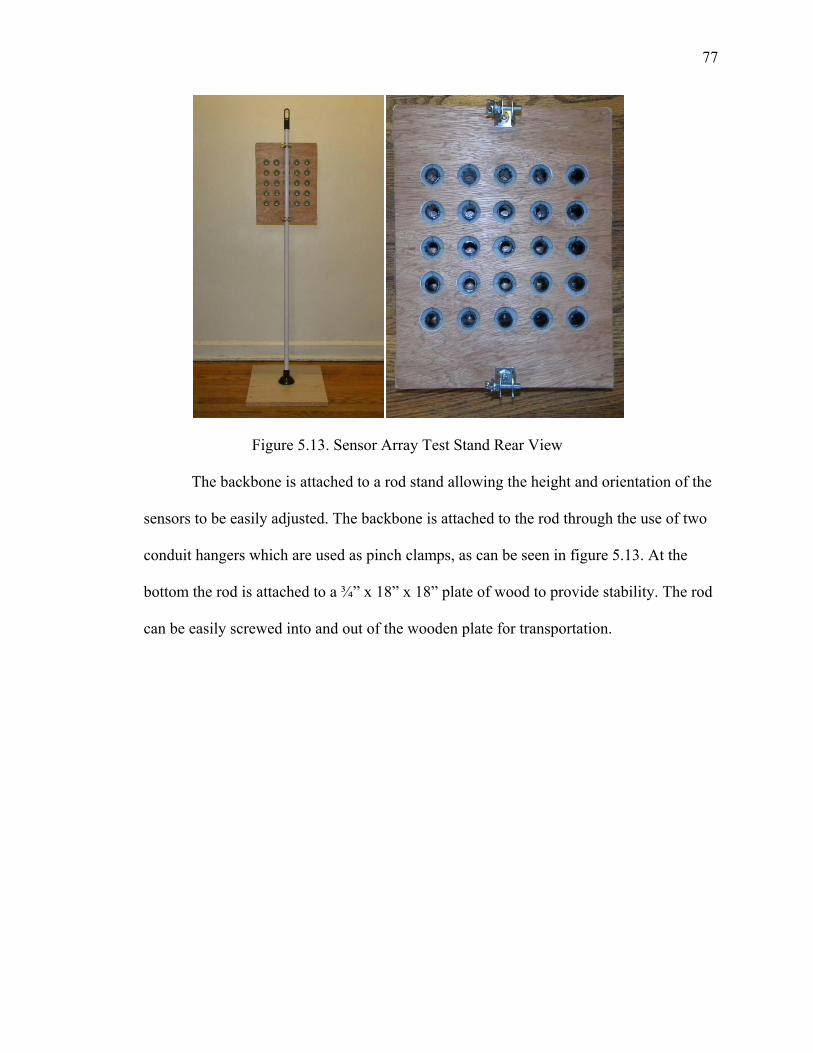
77
Figure 5.13. Sensor Array Test Stand Rear View
The backbone is attached to a rod stand allowing the height and orientation of the
sensors to be easily adjusted. The backbone is attached to the rod through the use of two
conduit hangers which are used as pinch clamps, as can be seen in figure 5.13. At the
bottom the rod is attached to a ¾” x 18” x 18” plate of wood to provide stability. The rod
can be easily screwed into and out of the wooden plate for transportation.
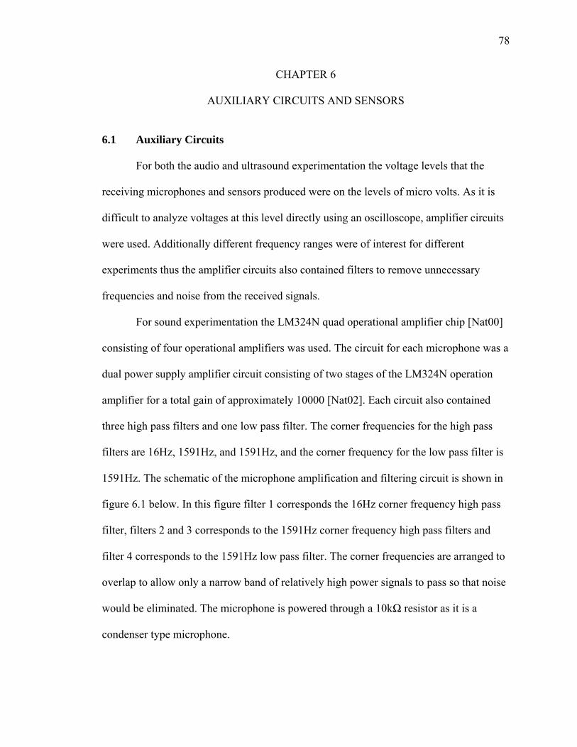
78
CHAPTER 6
AUXILIARY CIRCUITS AND SENSORS
6.1 Auxiliary Circuits
For both the audio and ultrasound experimentation the voltage levels that the
receiving microphones and sensors produced were on the levels of micro volts. As it is
difficult to analyze voltages at this level directly using an oscilloscope, amplifier circuits
were used. Additionally different frequency ranges were of interest for different
experiments thus the amplifier circuits also contained filters to remove unnecessary
frequencies and noise from the received signals.
For sound experimentation the LM324N quad operational amplifier chip [Nat00]
consisting of four operational amplifiers was used. The circuit for each microphone was a
dual power supply amplifier circuit consisting of two stages of the LM324N operation
amplifier for a total gain of approximately 10000 [Nat02]. Each circuit also contained
three high pass filters and one low pass filter. The corner frequencies for the high pass
filters are 16Hz, 1591Hz, and 1591Hz, and the corner frequency for the low pass filter is
1591Hz. The schematic of the microphone amplification and filtering circuit is shown in
figure 6.1 below. In this figure filter 1 corresponds the 16Hz corner frequency high pass
filter, filters 2 and 3 corresponds to the 1591Hz corner frequency high pass filters and
filter 4 corresponds to the 1591Hz low pass filter. The corner frequencies are arranged to
overlap to allow only a narrow band of relatively high power signals to pass so that noise
would be eliminated. The microphone is powered through a 10kΩ resistor as it is a
condenser type microphone.
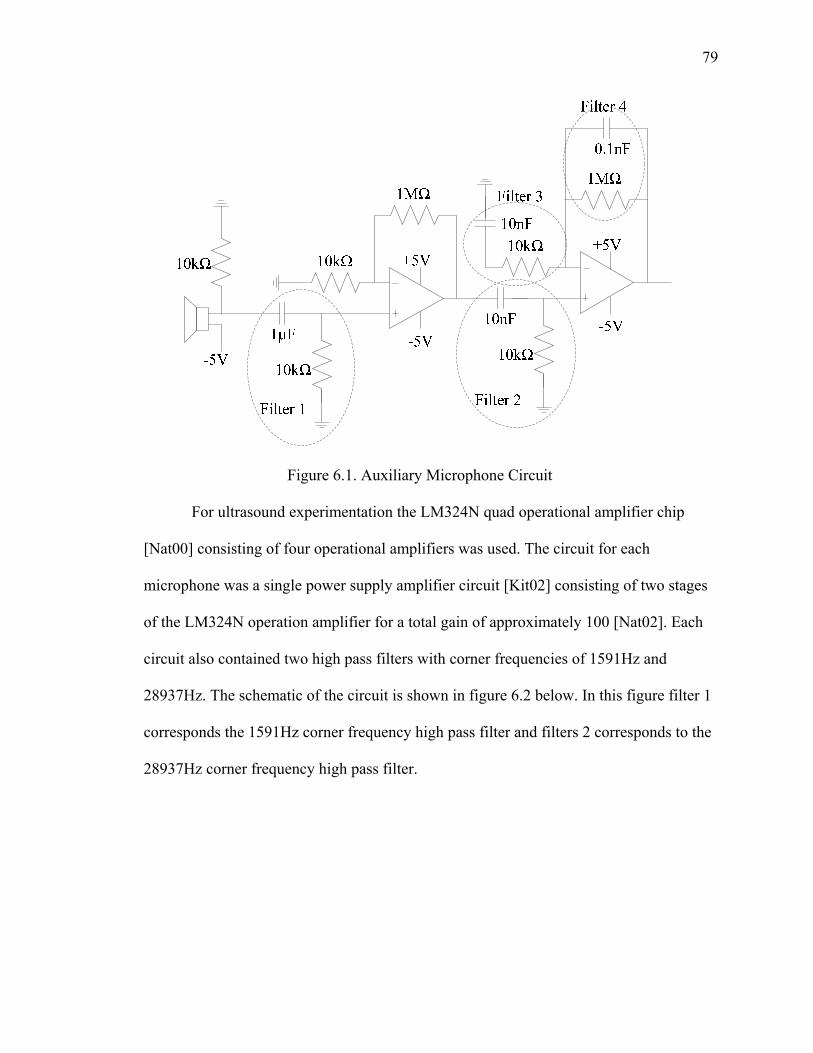
79
Figure 6.1. Auxiliary Microphone Circuit
For ultrasound experimentation the LM324N quad operational amplifier chip
[Nat00] consisting of four operational amplifiers was used. The circuit for each
microphone was a single power supply amplifier circuit [Kit02] consisting of two stages
of the LM324N operation amplifier for a total gain of approximately 100 [Nat02]. Each
circuit also contained two high pass filters with corner frequencies of 1591Hz and
28937Hz. The schematic of the circuit is shown in figure 6.2 below. In this figure filter 1
corresponds the 1591Hz corner frequency high pass filter and filters 2 corresponds to the
28937Hz corner frequency high pass filter.
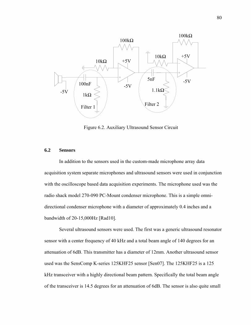
80
100nF
1kΩ
+5V
-5V
100kΩ
10kΩ+5V
-5V
100kΩ
10kΩ
5nF
1.1kΩ-5V
Filter 1Filter 2
Figure 6.2. Auxiliary Ultrasound Sensor Circuit
6.2 Sensors
In addition to the sensors used in the custom-made microphone array data
acquisition system separate microphones and ultrasound sensors were used in conjunction
with the oscilloscope based data acquisition experiments. The microphone used was the
radio shack model 270-090 PC-Mount condenser microphone. This is a simple omni-
directional condenser microphone with a diameter of approximately 0.4 inches and a
bandwidth of 20-15,000Hz [Rad10].
Several ultrasound sensors were used. The first was a generic ultrasound resonator
sensor with a center frequency of 40 kHz and a total beam angle of 140 degrees for an
attenuation of 6dB. This transmitter has a diameter of 12mm. Another ultrasound sensor
used was the SensComp K-series 125KHF25 sensor [Sen07]. The 125KHF25 is a 125
kHz transceiver with a highly directional beam pattern. Specifically the total beam angle
of the transceiver is 14.5 degrees for an attenuation of 6dB. The sensor is also quite small
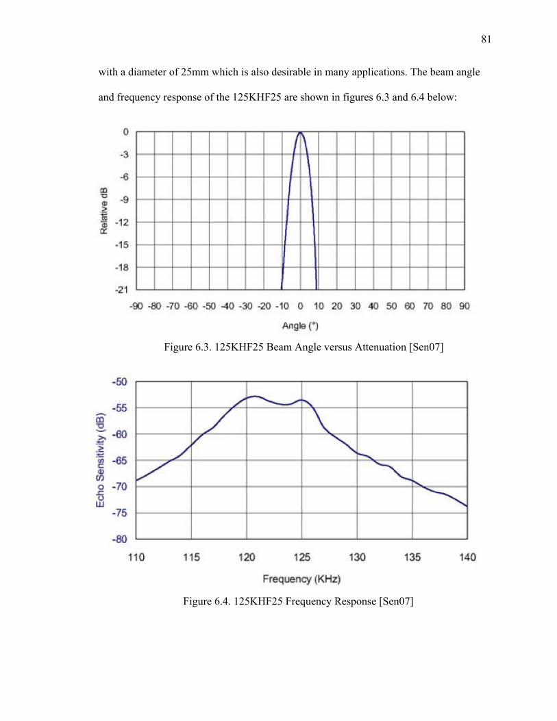
81
with a diameter of 25mm which is also desirable in many applications. The beam angle
and frequency response of the 125KHF25 are shown in figures 6.3 and 6.4 below:
Figure 6.3. 125KHF25 Beam Angle versus Attenuation [Sen07]
Figure 6.4. 125KHF25 Frequency Response [Sen07]
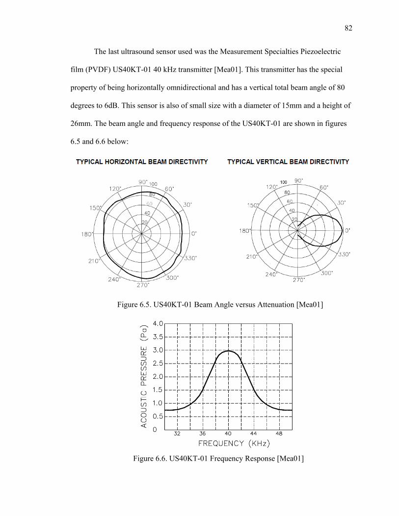
82
The last ultrasound sensor used was the Measurement Specialties Piezoelectric
film (PVDF) US40KT-01 40 kHz transmitter [Mea01]. This transmitter has the special
property of being horizontally omnidirectional and has a vertical total beam angle of 80
degrees to 6dB. This sensor is also of small size with a diameter of 15mm and a height of
26mm. The beam angle and frequency response of the US40KT-01 are shown in figures
6.5 and 6.6 below:
Figure 6.5. US40KT-01 Beam Angle versus Attenuation [Mea01]
Figure 6.6. US40KT-01 Frequency Response [Mea01]
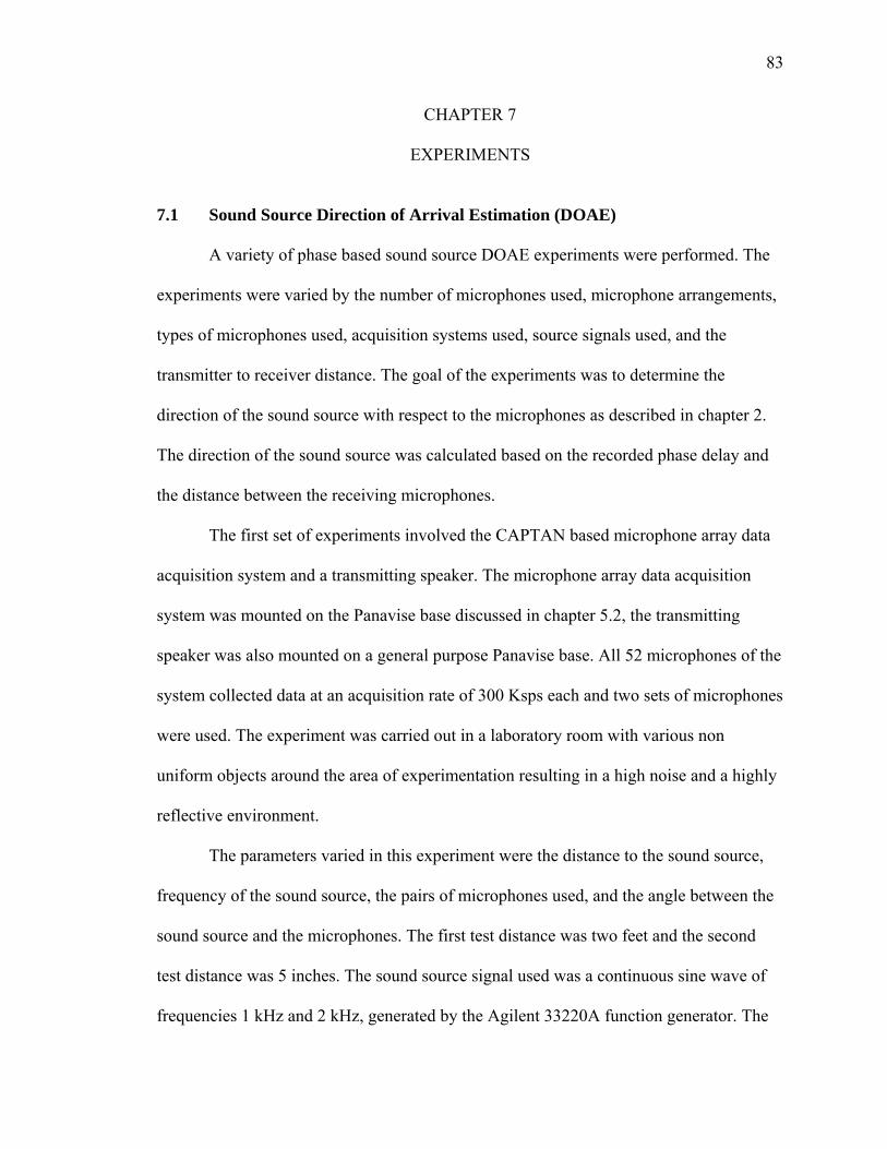
83
CHAPTER 7
EXPERIMENTS
7.1 Sound Source Direction of Arrival Estimation (DOAE)
A variety of phase based sound source DOAE experiments were performed. The
experiments were varied by the number of microphones used, microphone arrangements,
types of microphones used, acquisition systems used, source signals used, and the
transmitter to receiver distance. The goal of the experiments was to determine the
direction of the sound source with respect to the microphones as described in chapter 2.
The direction of the sound source was calculated based on the recorded phase delay and
the distance between the receiving microphones.
The first set of experiments involved the CAPTAN based microphone array data
acquisition system and a transmitting speaker. The microphone array data acquisition
system was mounted on the Panavise base discussed in chapter 5.2, the transmitting
speaker was also mounted on a general purpose Panavise base. All 52 microphones of the
system collected data at an acquisition rate of 300 Ksps each and two sets of microphones
were used. The experiment was carried out in a laboratory room with various non
uniform objects around the area of experimentation resulting in a high noise and a highly
reflective environment.
The parameters varied in this experiment were the distance to the sound source,
frequency of the sound source, the pairs of microphones used, and the angle between the
sound source and the microphones. The first test distance was two feet and the second
test distance was 5 inches. The sound source signal used was a continuous sine wave of
frequencies 1 kHz and 2 kHz, generated by the Agilent 33220A function generator. The
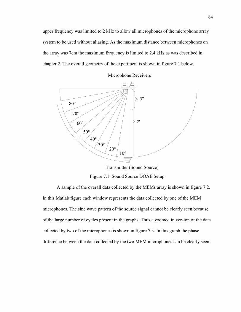
84
upper frequency was limited to 2 kHz to allow all microphones of the microphone array
system to be used without aliasing. As the maximum distance between microphones on
the array was 7cm the maximum frequency is limited to 2.4 kHz as was described in
chapter 2. The overall geometry of the experiment is shown in figure 7.1 below.
10°20°
30°40°
50°
60°
70°
80°
Microphone Receivers
Transmitter (Sound Source)
5"
2'
Figure 7.1. Sound Source DOAE Setup
A sample of the overall data collected by the MEMs array is shown in figure 7.2.
In this Matlab figure each window represents the data collected by one of the MEM
microphones. The sine wave pattern of the source signal cannot be clearly seen because
of the large number of cycles present in the graphs. Thus a zoomed in version of the data
collected by two of the microphones is shown in figure 7.3. In this graph the phase
difference between the data collected by the two MEM microphones can be clearly seen.
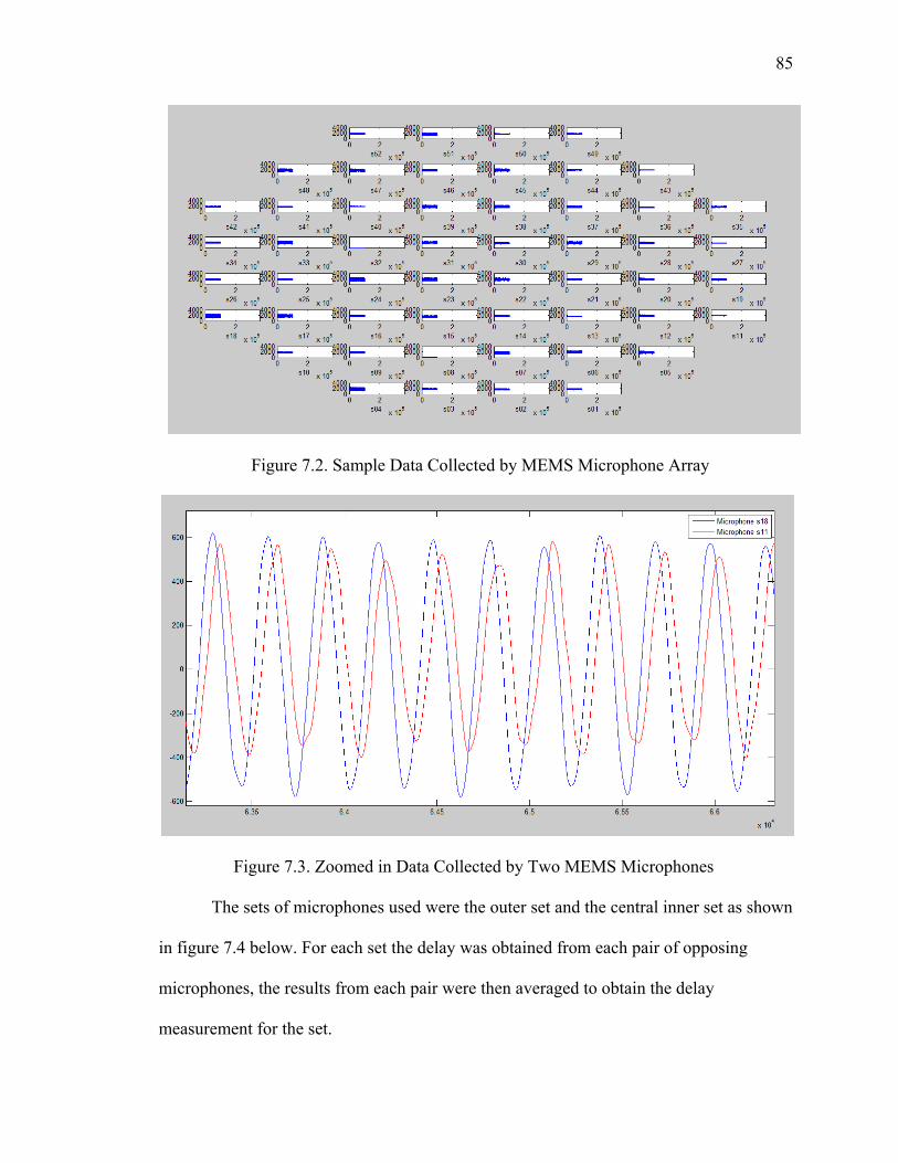
85
Figure 7.2. Sample Data Collected by MEMS Microphone Array
Figure 7.3. Zoomed in Data Collected by Two MEMS Microphones
The sets of microphones used were the outer set and the central inner set as shown
in figure 7.4 below. For each set the delay was obtained from each pair of opposing
microphones, the results from each pair were then averaged to obtain the delay
measurement for the set.
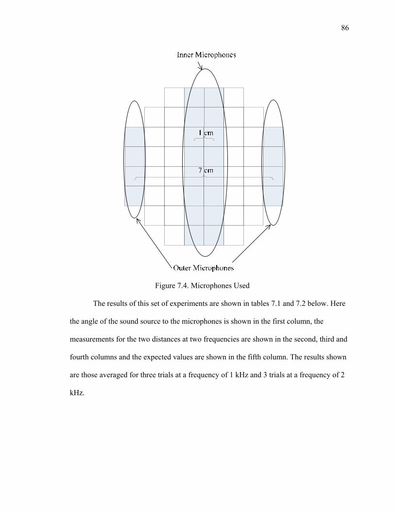
86
Figure 7.4. Microphones Used
The results of this set of experiments are shown in tables 7.1 and 7.2 below. Here
the angle of the sound source to the microphones is shown in the first column, the
measurements for the two distances at two frequencies are shown in the second, third and
fourth columns and the expected values are shown in the fifth column. The results shown
are those averaged for three trials at a frequency of 1 kHz and 3 trials at a frequency of 2
kHz.

87
Table 7.1. Sound Source DOAE Experiment Set 1, Outer Microphones Results
Outer Microphones Obtained Delay (ms) Theoretical
(Expected) Delay (ms) Angle (°)
2' Distance 5" Distance 1 kHz 2 kHz 1 kHz 2 kHz
0 -0.007 0.011 0 0.005 0 10 0.020 0.087 0.036 0.032 0.035 20 0.120 0.062 0.065 0.063 0.070 30 0.065 0.087 0.099 0.109 0.101 40 0.113 0.163 0.124 0.119 0.130 50 0.182 0.054 0.144 0.128 0.156 60 0.146 0.123 0.179 0.145 0.176 70 0.187 0.183 0.185 0.188 0.191 80 0.192 0.188 0.202 0.197 0.200
Table 7.2. Sound Source DOAE Experiment Set 1, Inner Microphones Results
Inner Microphones Obtained Delay (ms) Theoretical
(Expected) Delay (ms) Angle (°)
2' Distance 5" Distance 1 kHz 2 kHz 1 kHz 2 kHz
0 0.002 -0.03 0 0 0 10 0.000 0.003 0.004 0.004 0.005 20 0.016 0.018 0.011 0.010 0.010 30 0.018 0.013 0.015 0.012 0.014 40 0.016 00.15 0.019 0.016 0.018 50 0.021 0.018 0.020 0.024 0.022 60 0.021 0.019 0.024 0.026 0.025 70 0.029 0.0.29 0.026 0.028 0.027 80 0.027 0.030 0.027 0.028 0.028
It can be seen from these results that phase based DOAE in a highly noisy and
reverberant environment does not produce reliable results at larger distances independent
of the frequency of the source signal or the distance between the receiving microphones.
This can be seen from the mismatch between the collected data and the expected results,

88
and also from the fact that the time delays increase and decrease instead of just increasing
when the angle between the sound source and receiving microphones increases. It can
also be seen that phase based DOAE works better at close distances where the power of
the original signal is high compared to the power of the reflection based noise.
In order to reduce the effect of reflection and ambient noise the second set of
experiments were carried out inside the acoustic chamber discussed in chapter 5. These
experiment also used the CAPTAN based microphone array data acquisition system and a
transmitting speaker. The experimental setup and the parameters varied were also the
same as in the first set of experiments except for the use of the acoustic chamber.
The results of this set of experiments are shown in tables 7.3 and 7.4 below. Here
the angle of the sound source to the microphones is shown in the first column, the
measurements for the two distances at two frequencies are shown in the second, third and
fourth columns and the expected values are shown in the fifth column. The results shown
are those averaged for three trials at a frequency of 1 kHz and 3 trials at a frequency of 2
kHz.
Table 7.3. Sound Source DOAE Experiment Set 2, Outer Microphones Results
Outer Microphones Obtained Delay (ms) Theoretical
(Expected) Delay (ms) Angle (°)
2' Distance 5" Distance 1 kHz 2 kHz 1 kHz 2 kHz
0 0.003 -0.005 0 0 0 10 0.015 0.012 0.034 0.035 0.035 20 0.045 0.040 0.068 0.069 0.070 30 0.064 0.077 0.102 0.101 0.101 40 0.060 0.064 0.131 0.132 0.130 50 0.067 0.071 0.153 0.157 0.156 60 0.130 0.121 0.176 0.178 0.176 70 0.180 0.176 0.193 0.189 0.191 80 0.190 0.193 0.199 0.201 0.200
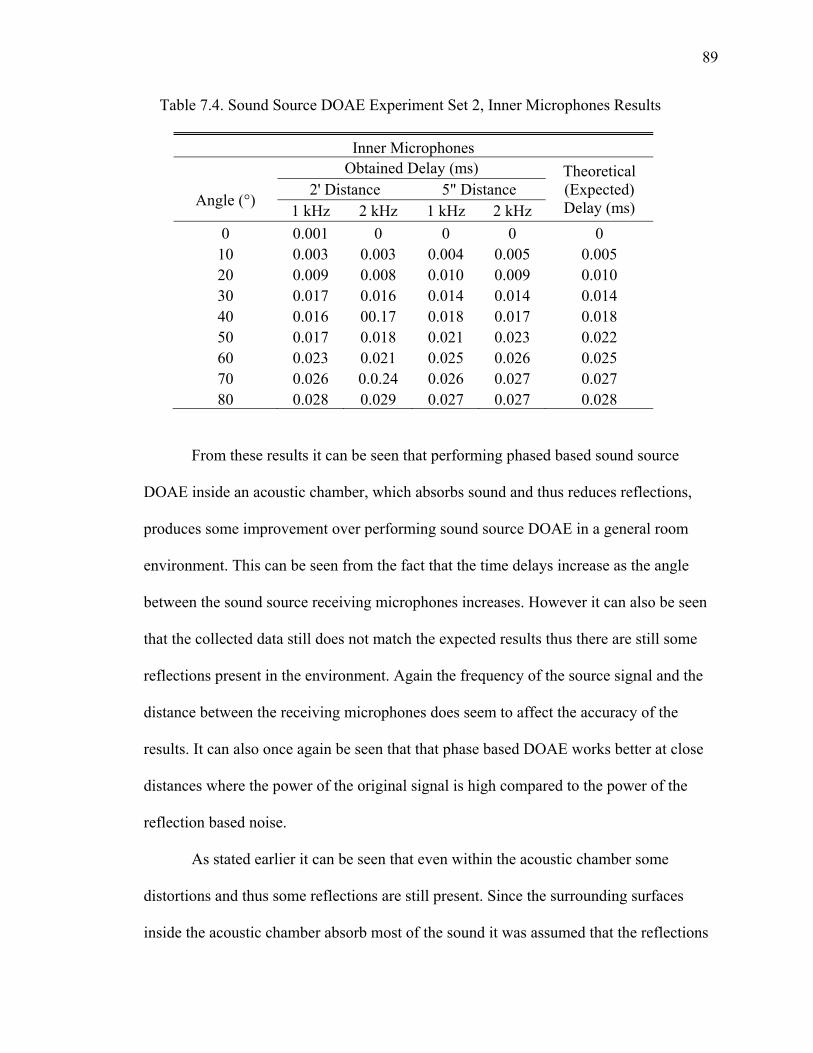
89
Table 7.4. Sound Source DOAE Experiment Set 2, Inner Microphones Results
Inner Microphones Obtained Delay (ms) Theoretical
(Expected) Delay (ms) Angle (°)
2' Distance 5" Distance 1 kHz 2 kHz 1 kHz 2 kHz
0 0.001 0 0 0 0 10 0.003 0.003 0.004 0.005 0.005 20 0.009 0.008 0.010 0.009 0.010 30 0.017 0.016 0.014 0.014 0.014 40 0.016 00.17 0.018 0.017 0.018 50 0.017 0.018 0.021 0.023 0.022 60 0.023 0.021 0.025 0.026 0.025 70 0.026 0.0.24 0.026 0.027 0.027 80 0.028 0.029 0.027 0.027 0.028
From these results it can be seen that performing phased based sound source
DOAE inside an acoustic chamber, which absorbs sound and thus reduces reflections,
produces some improvement over performing sound source DOAE in a general room
environment. This can be seen from the fact that the time delays increase as the angle
between the sound source receiving microphones increases. However it can also be seen
that the collected data still does not match the expected results thus there are still some
reflections present in the environment. Again the frequency of the source signal and the
distance between the receiving microphones does seem to affect the accuracy of the
results. It can also once again be seen that that phase based DOAE works better at close
distances where the power of the original signal is high compared to the power of the
reflection based noise.
As stated earlier it can be seen that even within the acoustic chamber some
distortions and thus some reflections are still present. Since the surrounding surfaces
inside the acoustic chamber absorb most of the sound it was assumed that the reflections

90
causing the distortions in this set of experiments came from the microphone array itself.
This is shown in figure 7.5 below.
Microphone Array
Original Sound Wave Sound Wave Reflections
Figure 7.5. Reflections from Microphone Array
In order to reduce the effect of the reflection coming from the microphone array
itself an alternate physical setup and acquisition system was used for the third set of
experiments. The physical setup consisted of the Panavise vise with a radio shack
microphone, described in chapter 6 section 2, attached to each of the two arms of the vise
through foam and with nothing in between the vise arms. This setup is shown figures 5.9
and 5.10. Foam was used to hold the microphones to further suppress the reflections from
one side of the mount to another and to prevent vibration coupling between the two
microphones. In this setup the distance between the microphones was 16 cm. Since there
was nothing between the microphones there was nothing to create reflections waves
except the foam wrapped arms of the vise itself.
The acquisition system used for this series of experiments was the Agilent
MSO6032A oscilloscope. Since a clear signal could not be obtained directly from the
microphones an amplification and filtering circuit as discussed in chapter 6 section 1 was
used for each microphone. The sound source signal was once again a continuous sine
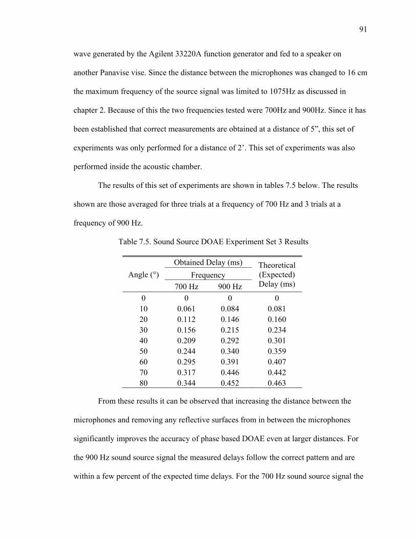
91
wave generated by the Agilent 33220A function generator and fed to a speaker on
another Panavise vise. Since the distance between the microphones was changed to 16 cm
the maximum frequency of the source signal was limited to 1075Hz as discussed in
chapter 2. Because of this the two frequencies tested were 700Hz and 900Hz. Since it has
been established that correct measurements are obtained at a distance of 5”, this set of
experiments was only performed for a distance of 2’. This set of experiments was also
performed inside the acoustic chamber.
The results of this set of experiments are shown in tables 7.5 below. The results
shown are those averaged for three trials at a frequency of 700 Hz and 3 trials at a
frequency of 900 Hz.
Table 7.5. Sound Source DOAE Experiment Set 3 Results
Angle (°)
Obtained Delay (ms) Theoretical (Expected) Delay (ms)
Frequency
700 Hz 900 Hz
0 0 0 0 10 0.061 0.084 0.081 20 0.112 0.146 0.160 30 0.156 0.215 0.234 40 0.209 0.292 0.301 50 0.244 0.340 0.359 60 0.295 0.391 0.407 70 0.317 0.446 0.442 80 0.344 0.452 0.463
From these results it can be observed that increasing the distance between the
microphones and removing any reflective surfaces from in between the microphones
significantly improves the accuracy of phase based DOAE even at larger distances. For
the 900 Hz sound source signal the measured delays follow the correct pattern and are
within a few percent of the expected time delays. For the 700 Hz sound source signal the

92
measured delays also follow the correct pattern but the delays are a reduced version of
the expected values, i.e. each measured delay is approximately 75% of the expected
value. Thus the frequency of the sound source signal now has some effects on the
measured time delay. This is again attributed to the remaining reflection in the
environment.
To further reduce the effects of reflection on the DOAE another set of
experiments was performed. Here the physical setup and the parameters varied were the
same as for the third set of experiments except for the type of source signal used. This
time instead of using a continuous sine wave for the source signal only 20 cycles of a sine
wave were transmitted. Then when this sine pulse train wave was received only the first
pulse was used for phase comparison. This was expected to further reduce errors due to
reflections since the first pulse should arrive before all reflections and thus its phase
information should not be distorted. A sample of the data collected for this set of
experiments is shown in figure 7.6.
Figure 7.6. Sound Source DOAE Experiment Set 4 Sample Results
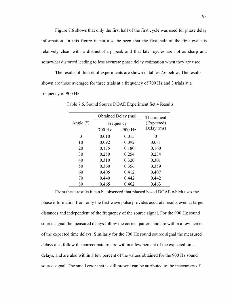
93
Figure 7.6 shows that only the first half of the first cycle was used for phase delay
information. In this figure it can also be seen that the first half of the first cycle is
relatively clean with a distinct sharp peak and that later cycles are not as sharp and
somewhat distorted leading to less accurate phase delay estimation when they are used.
The results of this set of experiments are shown in tables 7.6 below. The results
shown are those averaged for three trials at a frequency of 700 Hz and 3 trials at a
frequency of 900 Hz.
Table 7.6. Sound Source DOAE Experiment Set 4 Results
Angle (°)
Obtained Delay (ms) Theoretical (Expected) Delay (ms)
Frequency
700 Hz 900 Hz
0 0.010 0.015 0 10 0.092 0.092 0.081 20 0.175 0.180 0.160 30 0.250 0.254 0.234 40 0.310 0.320 0.301 50 0.360 0.356 0.359 60 0.405 0.412 0.407 70 0.440 0.442 0.442 80 0.465 0.462 0.463
From these results it can be observed that phased based DOAE which uses the
phase information from only the first wave pulse provides accurate results even at larger
distances and independent of the frequency of the source signal. For the 900 Hz sound
source signal the measured delays follow the correct pattern and are within a few percent
of the expected time delays. Similarly for the 700 Hz sound source signal the measured
delays also follow the correct pattern, are within a few percent of the expected time
delays, and are also within a few percent of the values obtained for the 900 Hz sound
source signal. The small error that is still present can be attributed to the inaccuracy of

94
the positioning of the sound source with respect to the receiving microphones, i.e. the
sound source is not placed exactly at 10° but possibly at 9.5° or 12°. This hypothesis
agrees with the data as the error gets smaller when then angle between the sound source
and microphones gets larger and thus the resultant distance between the sound source and
the speakers becomes less sensitive to positioning inaccuracies.
7.2 Ultrasound Matched Filter
Several ultrasound matched filter based experiments were performed. The
experiments were aimed at showing how using matched filtering could improve the
reliability for ultrasound ranging and how several signals may be localized at the same
time. The experiments consisted of creating different types of random signals,
transmitting them, capturing them, and then performing cross-correlation between the
transmitted and captured signals to determine either the distance to an object or to detect
the presence of a specific signal. The ultrasound transducers used were the SensComp
125KHF25 125 kHz transducers. The signals were generated in Matlab and transferred to
the Agilent 33220A function generator using the methods described in chapter 4. The
acquisition system used consisted of the Agilent MSO6032 oscilloscope and the
ultrasound sensor amplification circuit described in chapter 6.
Since most ultrasound transducers are resonators designed to only work in a very
narrow band of frequencies and having the optimum performance at their one central
frequency not all of the parameter typically used to create a matched filter template can
be used for ultrasound matched filtering. The frequency cannot be varied for typical
ultrasound transducer matched filtering for the reasons described above. The shape of
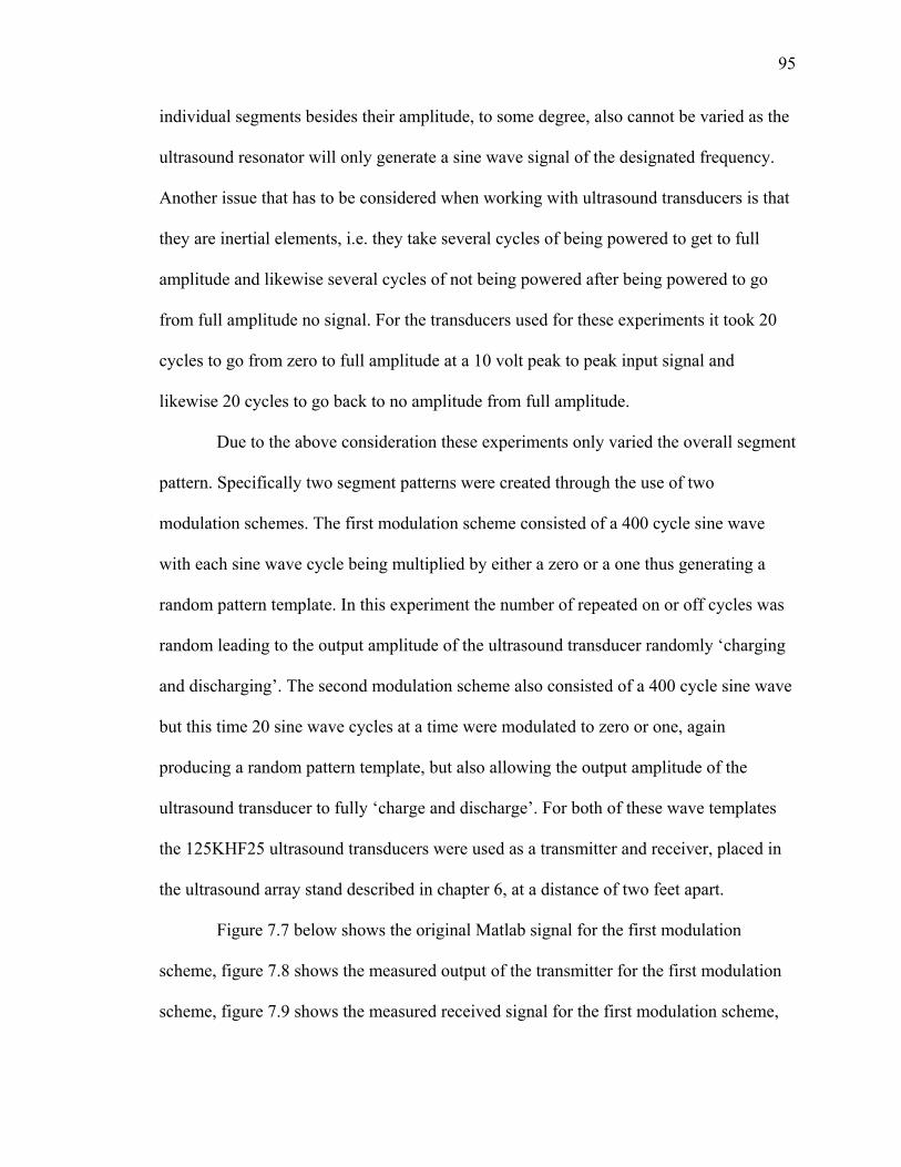
95
individual segments besides their amplitude, to some degree, also cannot be varied as the
ultrasound resonator will only generate a sine wave signal of the designated frequency.
Another issue that has to be considered when working with ultrasound transducers is that
they are inertial elements, i.e. they take several cycles of being powered to get to full
amplitude and likewise several cycles of not being powered after being powered to go
from full amplitude no signal. For the transducers used for these experiments it took 20
cycles to go from zero to full amplitude at a 10 volt peak to peak input signal and
likewise 20 cycles to go back to no amplitude from full amplitude.
Due to the above consideration these experiments only varied the overall segment
pattern. Specifically two segment patterns were created through the use of two
modulation schemes. The first modulation scheme consisted of a 400 cycle sine wave
with each sine wave cycle being multiplied by either a zero or a one thus generating a
random pattern template. In this experiment the number of repeated on or off cycles was
random leading to the output amplitude of the ultrasound transducer randomly ‘charging
and discharging’. The second modulation scheme also consisted of a 400 cycle sine wave
but this time 20 sine wave cycles at a time were modulated to zero or one, again
producing a random pattern template, but also allowing the output amplitude of the
ultrasound transducer to fully ‘charge and discharge’. For both of these wave templates
the 125KHF25 ultrasound transducers were used as a transmitter and receiver, placed in
the ultrasound array stand described in chapter 6, at a distance of two feet apart.
Figure 7.7 below shows the original Matlab signal for the first modulation
scheme, figure 7.8 shows the measured output of the transmitter for the first modulation
scheme, figure 7.9 shows the measured received signal for the first modulation scheme,
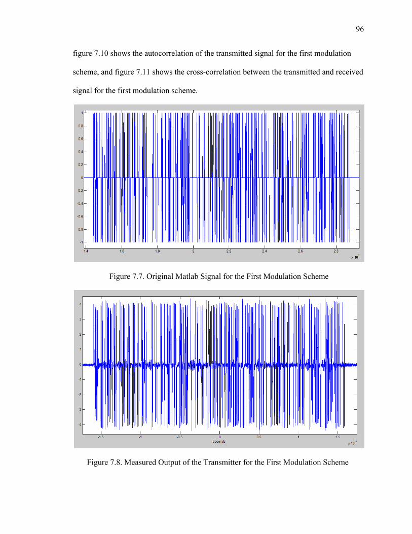
96
figure 7.10 shows the autocorrelation of the transmitted signal for the first modulation
scheme, and figure 7.11 shows the cross-correlation between the transmitted and received
signal for the first modulation scheme.
Figure 7.7. Original Matlab Signal for the First Modulation Scheme
Figure 7.8. Measured Output of the Transmitter for the First Modulation Scheme
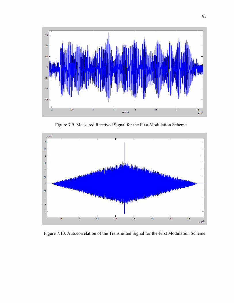
97
Figure 7.9. Measured Received Signal for the First Modulation Scheme
Figure 7.10. Autocorrelation of the Transmitted Signal for the First Modulation Scheme
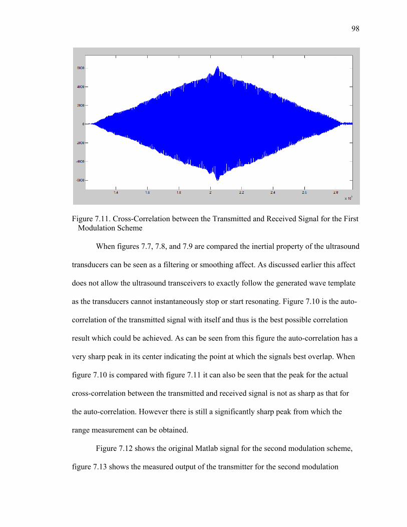
98
Figure 7.11. Cross-Correlation between the Transmitted and Received Signal for the First Modulation Scheme
When figures 7.7, 7.8, and 7.9 are compared the inertial property of the ultrasound
transducers can be seen as a filtering or smoothing affect. As discussed earlier this affect
does not allow the ultrasound transceivers to exactly follow the generated wave template
as the transducers cannot instantaneously stop or start resonating. Figure 7.10 is the auto-
correlation of the transmitted signal with itself and thus is the best possible correlation
result which could be achieved. As can be seen from this figure the auto-correlation has a
very sharp peak in its center indicating the point at which the signals best overlap. When
figure 7.10 is compared with figure 7.11 it can also be seen that the peak for the actual
cross-correlation between the transmitted and received signal is not as sharp as that for
the auto-correlation. However there is still a significantly sharp peak from which the
range measurement can be obtained.
Figure 7.12 shows the original Matlab signal for the second modulation scheme,
figure 7.13 shows the measured output of the transmitter for the second modulation
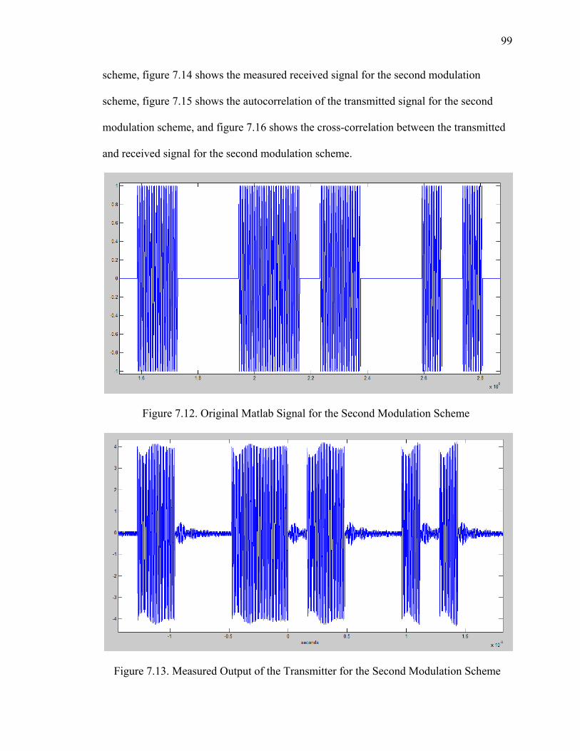
99
scheme, figure 7.14 shows the measured received signal for the second modulation
scheme, figure 7.15 shows the autocorrelation of the transmitted signal for the second
modulation scheme, and figure 7.16 shows the cross-correlation between the transmitted
and received signal for the second modulation scheme.
Figure 7.12. Original Matlab Signal for the Second Modulation Scheme
Figure 7.13. Measured Output of the Transmitter for the Second Modulation Scheme
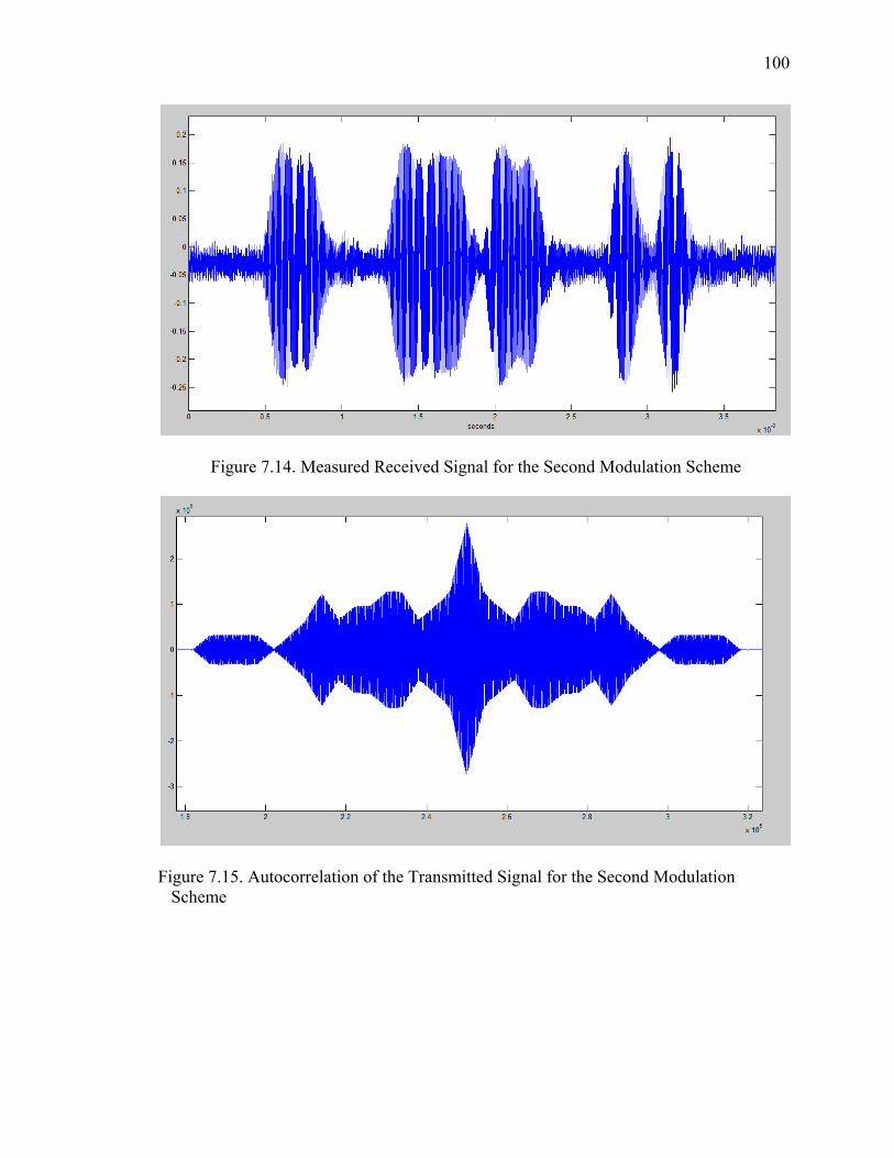
100
Figure 7.14. Measured Received Signal for the Second Modulation Scheme
Figure 7.15. Autocorrelation of the Transmitted Signal for the Second Modulation Scheme
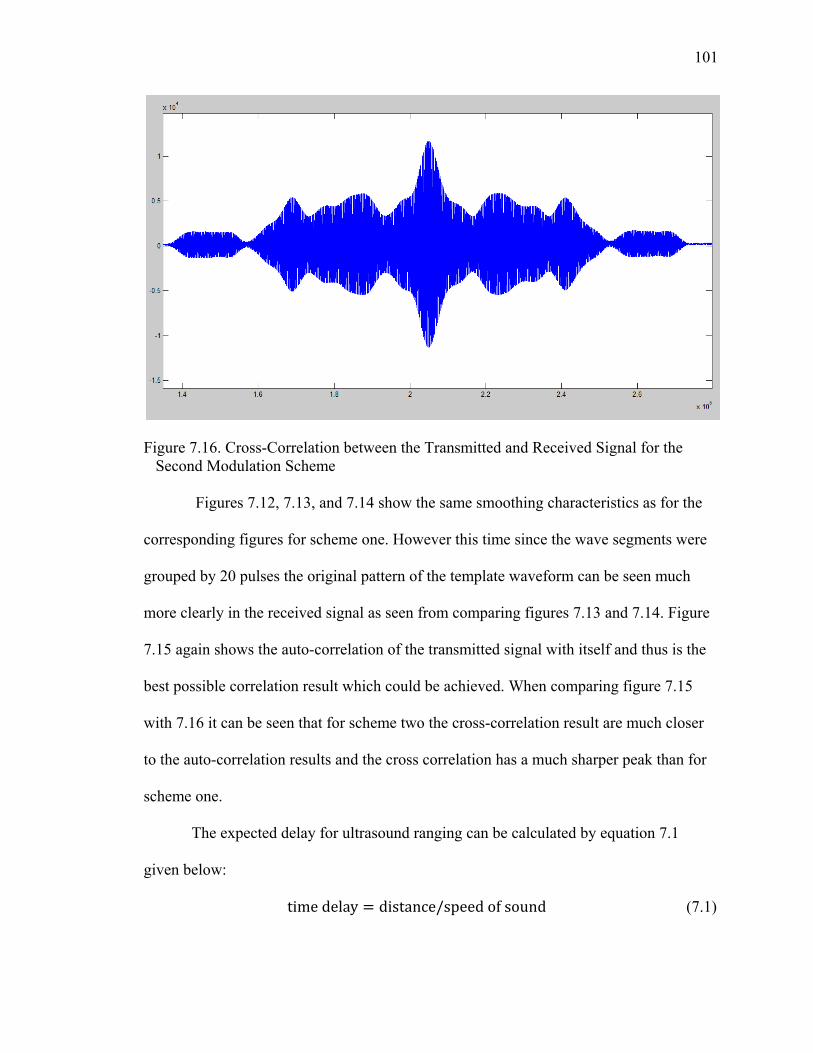
101
Figure 7.16. Cross-Correlation between the Transmitted and Received Signal for the Second Modulation Scheme
Figures 7.12, 7.13, and 7.14 show the same smoothing characteristics as for the
corresponding figures for scheme one. However this time since the wave segments were
grouped by 20 pulses the original pattern of the template waveform can be seen much
more clearly in the received signal as seen from comparing figures 7.13 and 7.14. Figure
7.15 again shows the auto-correlation of the transmitted signal with itself and thus is the
best possible correlation result which could be achieved. When comparing figure 7.15
with 7.16 it can be seen that for scheme two the cross-correlation result are much closer
to the auto-correlation results and the cross correlation has a much sharper peak than for
scheme one.
The expected delay for ultrasound ranging can be calculated by equation 7.1
given below:
time delay distance/speed of sound (7.1)

102
For the two feet distance used for this experiment the expected delay is given by
equation 7.2 below:
0.0018sec 0.6096/344 (7.2)
The collected time delays can be calculated from the cross-correlation results as
given by equation 7.3 below:
time delay = (size of signal array – index of peak point)*
*captured signal time length/size of signal array (7.3)
For both of the above used modulation schemes the results for this calculation
yielded 0.0018 seconds, exactly matching the expected delay. Thus the accuracy of both
of the match filters used is quite good. However as the second scheme produced a sharper
cross-correlation peak it may be more reliable in the presence of additional noise as the
higher and more separated peak will require more noise to make it indistinguishable from
surrounding peaks.
Figures 7.17 shows the cross-correlation between the transmitted signals of the
two schemes, figure 7.18 shows cross-correlation between the transmitted signal of the
first scheme and the received signal of the second scheme, figure 7.19 shows cross-
correlation between the transmitted signal of the second scheme and the received signal
of the first scheme, figure 7.20 shows cross-correlation between the transmitted second
scheme and a received combination of the first and second schemes.

103
Figure 7.17. Cross-Correlations between the Transmitted Signals of the Two Schemes
Figure 7.18. Cross-Correlation between the Transmitted Signal of the First Scheme and the Received Signal of the Second Scheme
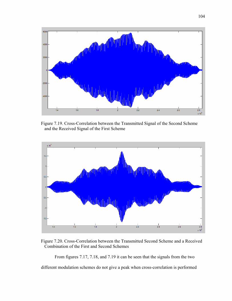
104
Figure 7.19. Cross-Correlation between the Transmitted Signal of the Second Scheme and the Received Signal of the First Scheme
Figure 7.20. Cross-Correlation between the Transmitted Second Scheme and a Received Combination of the First and Second Schemes
From figures 7.17, 7.18, and 7.19 it can be seen that the signals from the two
different modulation schemes do not give a peak when cross-correlation is performed
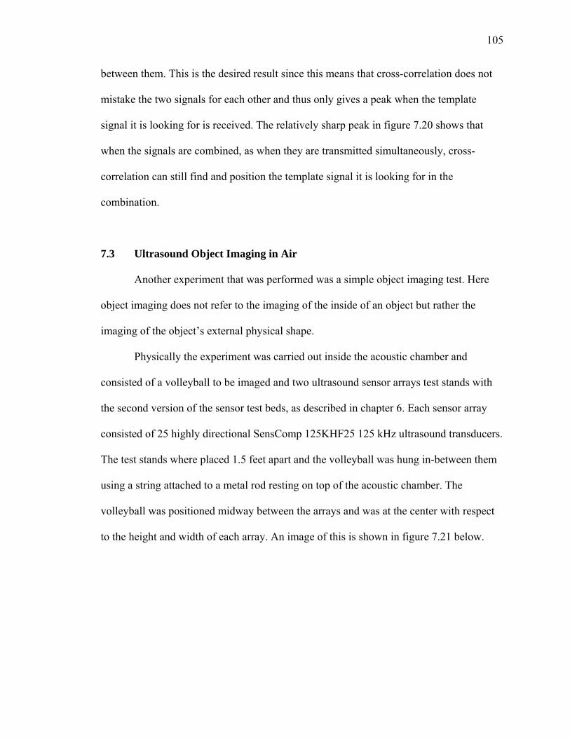
105
between them. This is the desired result since this means that cross-correlation does not
mistake the two signals for each other and thus only gives a peak when the template
signal it is looking for is received. The relatively sharp peak in figure 7.20 shows that
when the signals are combined, as when they are transmitted simultaneously, cross-
correlation can still find and position the template signal it is looking for in the
combination.
7.3 Ultrasound Object Imaging in Air
Another experiment that was performed was a simple object imaging test. Here
object imaging does not refer to the imaging of the inside of an object but rather the
imaging of the object’s external physical shape.
Physically the experiment was carried out inside the acoustic chamber and
consisted of a volleyball to be imaged and two ultrasound sensor arrays test stands with
the second version of the sensor test beds, as described in chapter 6. Each sensor array
consisted of 25 highly directional SensComp 125KHF25 125 kHz ultrasound transducers.
The test stands where placed 1.5 feet apart and the volleyball was hung in-between them
using a string attached to a metal rod resting on top of the acoustic chamber. The
volleyball was positioned midway between the arrays and was at the center with respect
to the height and width of each array. An image of this is shown in figure 7.21 below.
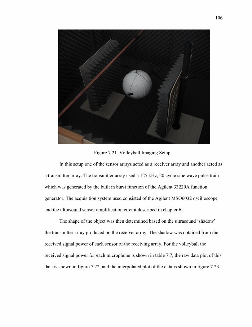
106
Figure 7.21. Volleyball Imaging Setup
In this setup one of the sensor arrays acted as a receiver array and another acted as
a transmitter array. The transmitter array used a 125 kHz, 20 cycle sine wave pulse train
which was generated by the built in burst function of the Agilent 33220A function
generator. The acquisition system used consisted of the Agilent MSO6032 oscilloscope
and the ultrasound sensor amplification circuit described in chapter 6.
The shape of the object was then determined based on the ultrasound ‘shadow’
the transmitter array produced on the receiver array. The shadow was obtained from the
received signal power of each sensor of the receiving array. For the volleyball the
received signal power for each microphone is shown in table 7.7, the raw data plot of this
data is shown in figure 7.22, and the interpolated plot of the data is shown in figure 7.23.
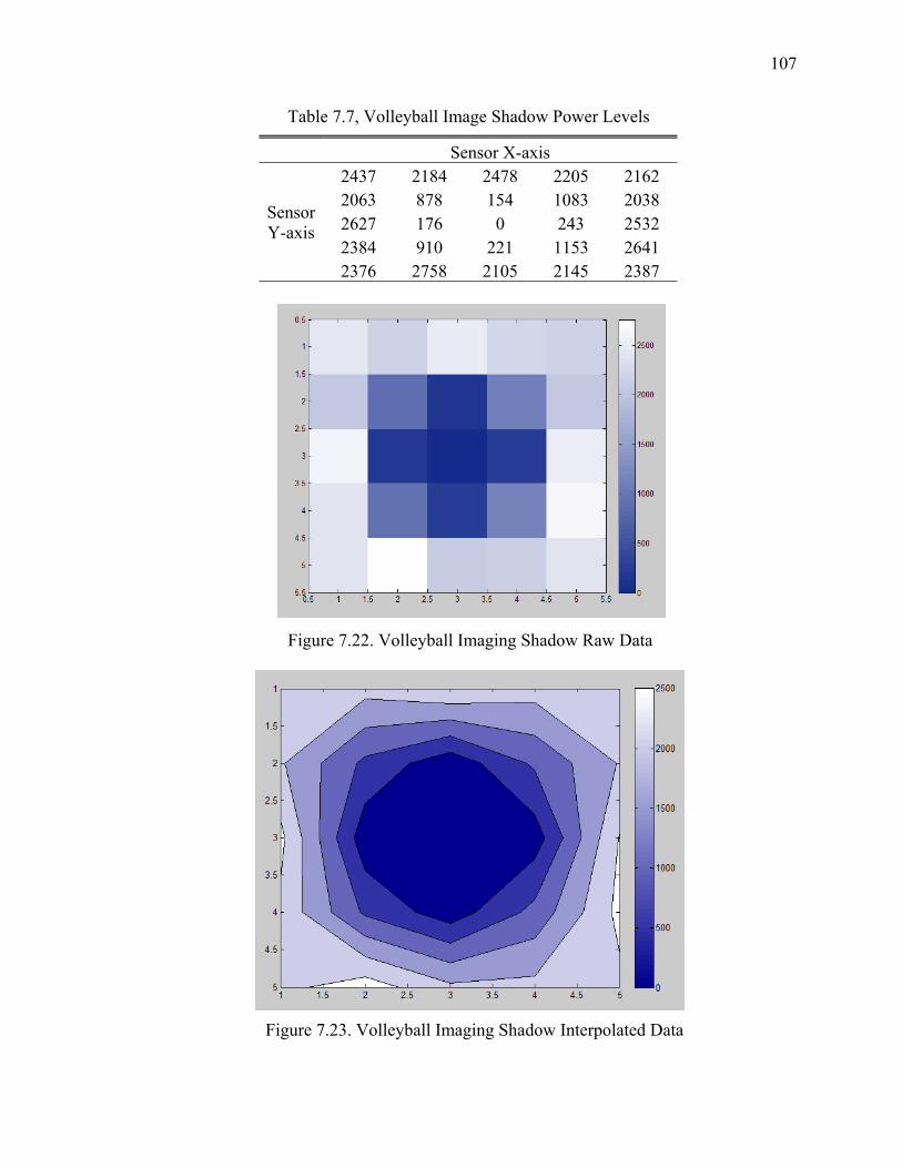
107
Table 7.7, Volleyball Image Shadow Power Levels
Sensor X-axis
Sensor Y-axis
2437 2184 2478 2205 2162 2063 878 154 1083 2038 2627 176 0 243 2532 2384 910 221 1153 2641 2376 2758 2105 2145 2387
Figure 7.22. Volleyball Imaging Shadow Raw Data
Figure 7.23. Volleyball Imaging Shadow Interpolated Data
108
From these results it can be seen that the overall shape of the object could be
extrapolated to some degree from the obtained power levels. The limitations of this
technique are that it only shows the projection of the object in one plane however this
could easily be expanded to a three plane projection using two more pairs of sensor
arrays. Another limitation is the resolution as can be seen from the poor approximation of
the ball in figure 7.23. This however could be improved by using more closely spaced
sensors, in which case only the size and directivity of the sensors will be the limiting
factor. Since ultrasonic sensors in the MHz range have both high directionality and small
sizes this is not an issue. The only other issue is that the projection of an object only
shows its outline and not necessarily its overall shape. Ranging with the sensor arrays
could be used to obtain the shape of an object to some degree however this could be
extremely complex as the surface of an object could be at various angles and could
scatter the ultrasound in several directions.
7.4 Ultrasound Localization
Two types of ultrasound source localization experiments were performed, the first
was a 2D ultrasound source localization experiment and the second was a 3D ultrasound
source localization experiment. For both types of experiments localization was performed
based on the delays corresponding to the receiver to transmitter distances and based on
the TDOA information between the receivers. As stated in chapter 2 the reason that both
the delay between transmission and reception and the TDOA between the receivers is
considered is because the delays between the transmission and reception may not always
be available since the time of transmission is not always known. However the time at
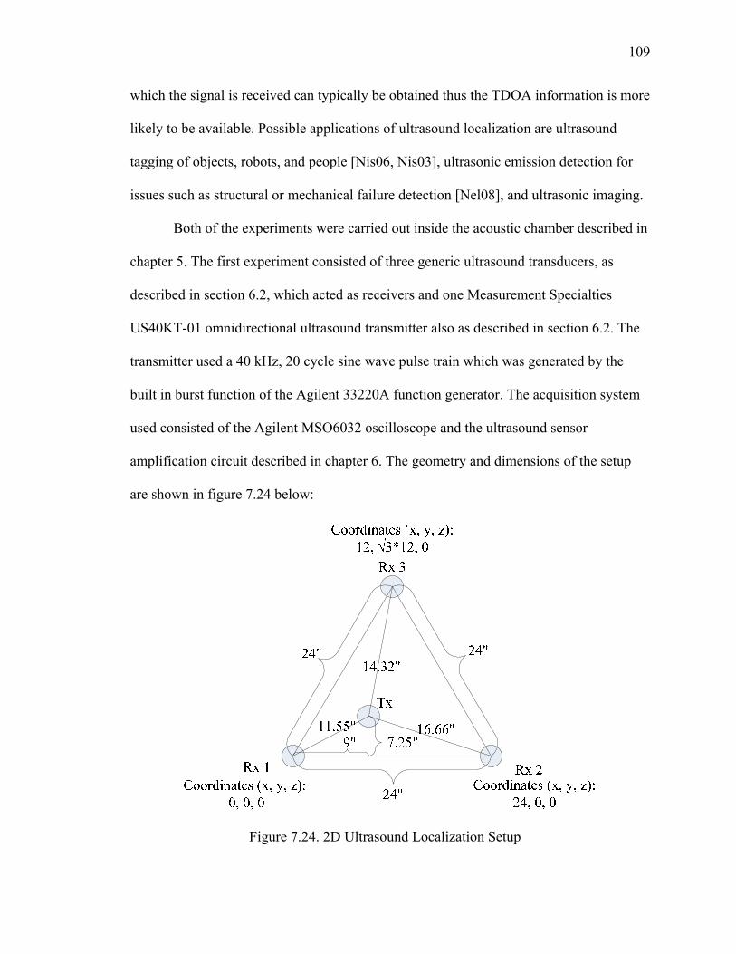
109
which the signal is received can typically be obtained thus the TDOA information is more
likely to be available. Possible applications of ultrasound localization are ultrasound
tagging of objects, robots, and people [Nis06, Nis03], ultrasonic emission detection for
issues such as structural or mechanical failure detection [Nel08], and ultrasonic imaging.
Both of the experiments were carried out inside the acoustic chamber described in
chapter 5. The first experiment consisted of three generic ultrasound transducers, as
described in section 6.2, which acted as receivers and one Measurement Specialties
US40KT-01 omnidirectional ultrasound transmitter also as described in section 6.2. The
transmitter used a 40 kHz, 20 cycle sine wave pulse train which was generated by the
built in burst function of the Agilent 33220A function generator. The acquisition system
used consisted of the Agilent MSO6032 oscilloscope and the ultrasound sensor
amplification circuit described in chapter 6. The geometry and dimensions of the setup
are shown in figure 7.24 below:
Figure 7.24. 2D Ultrasound Localization Setup
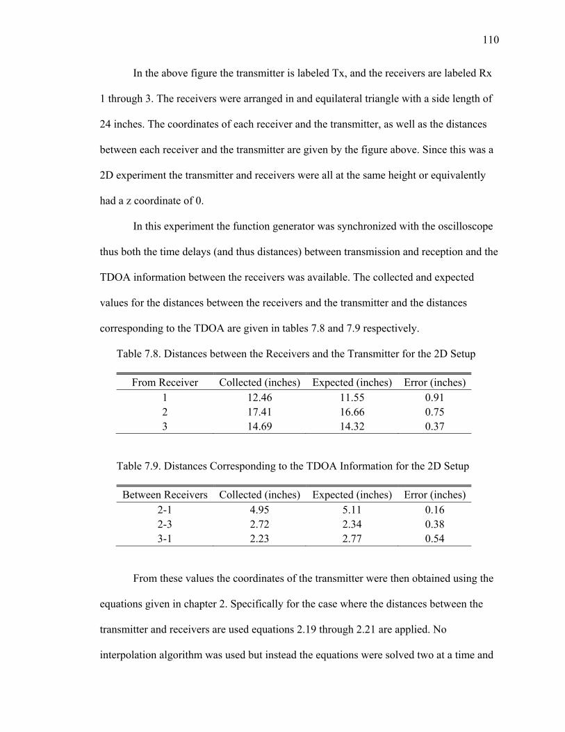
110
In the above figure the transmitter is labeled Tx, and the receivers are labeled Rx
1 through 3. The receivers were arranged in and equilateral triangle with a side length of
24 inches. The coordinates of each receiver and the transmitter, as well as the distances
between each receiver and the transmitter are given by the figure above. Since this was a
2D experiment the transmitter and receivers were all at the same height or equivalently
had a z coordinate of 0.
In this experiment the function generator was synchronized with the oscilloscope
thus both the time delays (and thus distances) between transmission and reception and the
TDOA information between the receivers was available. The collected and expected
values for the distances between the receivers and the transmitter and the distances
corresponding to the TDOA are given in tables 7.8 and 7.9 respectively.
Table 7.8. Distances between the Receivers and the Transmitter for the 2D Setup
From Receiver Collected (inches) Expected (inches) Error (inches) 1 12.46 11.55 0.91 2 17.41 16.66 0.75 3 14.69 14.32 0.37
Table 7.9. Distances Corresponding to the TDOA Information for the 2D Setup
Between Receivers Collected (inches) Expected (inches) Error (inches) 2-1 4.95 5.11 0.16 2-3 2.72 2.34 0.38 3-1 2.23 2.77 0.54
From these values the coordinates of the transmitter were then obtained using the
equations given in chapter 2. Specifically for the case where the distances between the
transmitter and receivers are used equations 2.19 through 2.21 are applied. No
interpolation algorithm was used but instead the equations were solved two at a time and
111
then the three pairs of results were averaged. For the case in which only the TDOA
information is used equations 2.19 through 2.23 are directly applied. The collected and
expected values for the coordinates of the transmitter based on the transmitter to receiver
distances and based on the TDOA information are given in tables 7.10 and 7.11
respectively.
Table 7.10. Transmitter Coordinates Based on Distances for the 2D Setup
Coordinate Collected (inches) Expected (inches) Error (inches) x 9.22 9 0.22 y 7.76 7.25 0.51
Table 7.11. Transmitter Coordinates Based on TDOA for the 2D Setup
Coordinate Collected (inches) Expected (inches) Error (inches) x 9.09 9 0.09 y 7.24 7.25 0.01
When interpreting the accuracy of these results it should also be considered that
the expected results themselves have an approximate error of +/- ½ inches due to
positioning errors. Thus from these results it can be seen that both methods give
relatively accurate approximations of the ultrasound transmitter’s coordinates, with the
TDOA based results being slightly more accurate.
The second experiment consisted of six generic ultrasound transducers as
described in section 6.2, five of which acted as receivers and one of which acted as a
transmitter. The transmitter used a 40 kHz, 20 cycle sine wave pulse train which was
generated by the built in burst function of the Agilent 33220A function generator. The
acquisition system used consisted of the Agilent MSO6032 oscilloscope and the
ultrasound sensor amplification circuit described in chapter 6. The first version of the
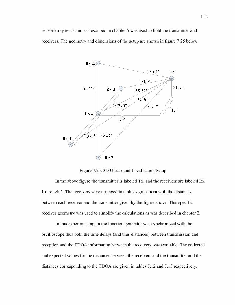
112
sensor array test stand as described in chapter 5 was used to hold the transmitter and
receivers. The geometry and dimensions of the setup are shown in figure 7.25 below:
Figure 7.25. 3D Ultrasound Localization Setup
In the above figure the transmitter is labeled Tx, and the receivers are labeled Rx
1 through 5. The receivers were arranged in a plus sign pattern with the distances
between each receiver and the transmitter given by the figure above. This specific
receiver geometry was used to simplify the calculations as was described in chapter 2.
In this experiment again the function generator was synchronized with the
oscilloscope thus both the time delays (and thus distances) between transmission and
reception and the TDOA information between the receivers was available. The collected
and expected values for the distances between the receivers and the transmitter and the
distances corresponding to the TDOA are given in tables 7.12 and 7.13 respectively.

113
Table 7.12. Distances between the Receivers and the Transmitter for the 3D Setup
From Receiver Collected (inches) Expected (inches) Error (inches) 1 37.921 37.26 0.661 2 37.378 36.71 0.668 3 34.807 34.04 0.767 4 35.213 34.61 0.603 5 36.567 35.53 1.037
Table 7.13. Distances Corresponding to the TDOA Information for the 3D Setup
Between Receivers Collected (inches) Expected (inches) Error (inches) 1-2 0.543 0.55 0.007 1-3 3.114 3.22 0.106 1-4 2.708 2.65 0.058 1-5 1.354 1.73 -0.376
From these values the coordinates of the transmitter were then obtained using the
equations given in chapter 2. Specifically for the case where the distances between the
transmitter and receivers are used the law of cosines was applied like shown with
equations 2.15 through 2.16. No interpolation algorithm was used but instead the two
equations were solved for each axis and the pairs of results were averaged. For the case in
which only the TDOA information is used equations 2.15 through 2.16 are directly
applied. The collected and expected values for the coordinates of the transmitter based on
the transmitter to receiver distances and based on the TDOA information are given in
tables 7.14 and 7.15 respectively.
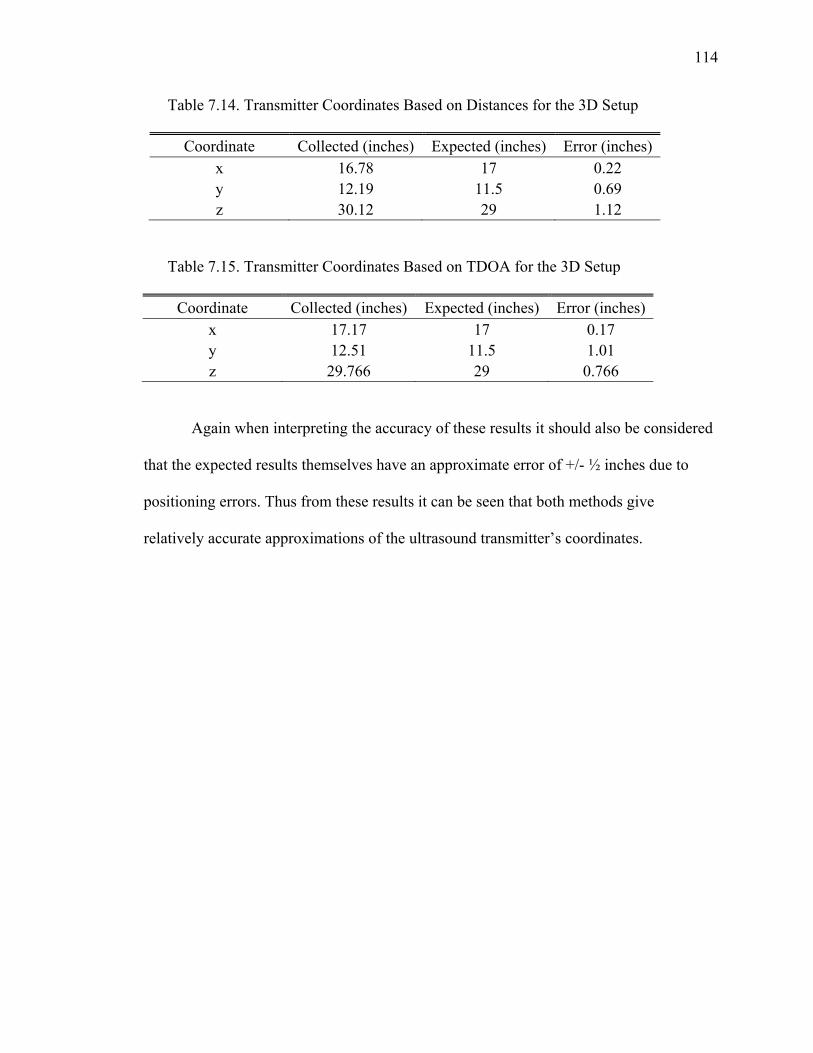
114
Table 7.14. Transmitter Coordinates Based on Distances for the 3D Setup
Coordinate Collected (inches) Expected (inches) Error (inches) x 16.78 17 0.22 y 12.19 11.5 0.69 z 30.12 29 1.12
Table 7.15. Transmitter Coordinates Based on TDOA for the 3D Setup
Coordinate Collected (inches) Expected (inches) Error (inches) x 17.17 17 0.17 y 12.51 11.5 1.01 z 29.766 29 0.766
Again when interpreting the accuracy of these results it should also be considered
that the expected results themselves have an approximate error of +/- ½ inches due to
positioning errors. Thus from these results it can be seen that both methods give
relatively accurate approximations of the ultrasound transmitter’s coordinates.
115
CHAPTER 8
CONCLUSION AND FUTURE WORK
8.1 Conclusion
In this work the fundamentals of 2D and 3D sound and ultrasound source
localization are presented. The topics of matched filtering, object imaging and how they
relate to ultrasound are also explored. A novel FPGA/MEMS based data acquisition and
microphone array system is presented and its utilization for the above described topics is
compared to standard test equipment and standard sensor based data acquisition systems.
In addition to this the capabilities of a generic data generation system (arbitrary
waveform generator) are also explored and its applications to signal generation for
DOAE, localization, matched filtering, and ranger are presented. The design of an
anechoic chamber, precision measurement mount, and several sensor array stands and
their utilization for the above described topics are described. Lastly several DOAE,
localization, matched filter, and ranging/imaging experiments are conducted using
various combinations of these concepts, designs, and equipment.
The fundamentals and variations of the DOAE and localization problem are
described to allow for a more complete understanding of the experiments and their
results. Specifically the difference between DOAE and localization were explained, the
differences between 2D and 3D scenarios were also explained and various parameters
such as the geometries, numbers of receivers, signal types, applicable algorithms, types of
information used and the minimum amount of information was considered. The types of
models used and the mathematics associated with them were derived and explained. The
steps used to perform DOAE and localization were presented and the differences between
116
ultrasound and sound methods were discussed. General considerations and limitations
such as the frequency and spatial sampling theorem, limitations on the types of models
which can be used, and the mathematical limitations were presented. The basics of
matched filtering and the improvements which could be obtained for DOAE, localization,
and ranging based on matched filtering were explained.
The FPGA/MEMS acquisition and microphone array system was described. This
consisted of the presentation of the three main physical boards (NPCB, GEL, and AMA)
and the core architecture (CAPTAN) behind the system. Specifically the three main parts
of the CAPTAN system, namely the node layer, the network layer, and the application
interface layer, were described. The design, features, and limitations of the system and
the architecture were explored. This included discussions of the CAPTAN based system’s
acquisition capabilities, networkability, high communication rates, modularity within
nodes and between nodes, modularity in configeware and software, ease of hardware and
software expandability, high processing power and the ability to perform PC based
processing.
In contrast to the custom FPGA/MEMS system, the capabilities and features of a
generic oscilloscope (MSO6032A) based data acquisition system were presented. The
main issues explored were the necessary auxiliary circuits for amplification and filtering,
techniques of interfacing with the oscilloscope, capturing and transferring data from the
oscilloscope to the PC and programming of the scope. The techniques explored included
front panel interface, data capture, and portable storage based transfer, built in
web/network interface, existing software, direct USB link based interface, data capture
and transfer, SCPI programming based interface, data capture and transfer, and driver
117
programming based interface, data capture and transfer. The advantages, such as speed
of use, ease of interface, and interchangeability, and the disadvantages, such as limited
number of channels and lack of real-time processing, were also presented. In addition to
this the generic data generation system (A33220A) was discussed and the various
techniques of interfacing with the waveform generator, creating arbitrary waveforms and
transferring arbitrary waveforms from the PC to the waveform generator were explored.
The acoustic chamber, measurement mount, and sensor array test stands were
created to allow the various experiments to be conducted in a more controlled manner.
The design and features of the acoustic chamber such as its modularity, expandability,
and acoustic absorption properties were described. The design and usage of the
measurement mount as it relates to the accuracy of source positioning for the localization
experiments was discuss. Lastly the design and features of the sensor array test stands
such as its adjustability, modularity, and its ability to allow for a large number of sensor
geometries to be experimented with were presented.
Four general types of experiments were conducted, specifically the types were
sound DOAE, ultrasound matched filtering, ultrasound object imaging, and ultrasound
source localization. The sound direction of arrival experiments showed how phased based
estimation can be performed, how the CAPTAN based system and generic acquisition
and generation systems can be utilized for these types of experiments. The results show
how the accuracy of the estimation is affected by various parameters such as the acoustic
chamber, the receiver geometries, frequencies used, distances between the transmitter and
receiver, and type of interpretation of the received signal.

118
The matched filter experiments demonstrated how matched filters could be
applied to ultrasound and how a generic data generation system could be used to create a
variety of useful waveforms. Specifically the matched filter experiment show how
different types of filters operate with ultrasound transducers, how these techniques could
be used to increase the accuracy of ranging, and how they can be used to simultaneously
send multiple transmission on the same medium.
The ultrasound object imaging experiment simply showed how ultrasound
ranging could be used for basic object shape/outline detection.
The ultrasound localization set of experiments demonstrate how 2D and 3D
localization can be performed based either the TDOA information or the receiver to
transmitter distance information. Several applications such as acoustic emission detection
and ultrasound tagging are discussed. The results demonstrate that the approaches used
give quite accurate positions of the sources for both 2D and 3D cases using either type of
information as inputs.
8.2 Future Work
Several steps can be taken in the future to improve this work. The
FPGA/CAPTAN based system may be modified to perform general data acquisition
across multiple sensors instead of data acquisition for specific types of microphones. This
modification would be relatively easy as it would simply involve modifying the AMA
board to have general input connectors instead of specific types of attached microphones.
Another direction that could be taken is the development of standardized
oscilloscope based data acquisition system through the use of interchangeable instrument
119
drivers. This would involve the creation of either a command line or GUI style software
which would use interchangeable instrument drivers to allow common commands to be
used to interface with the various oscilloscopes on the market.
The ultrasound object imaging series of experiments can also be significantly
expanded. Specifically ranging/sensor array based techniques could be explored for the
possibility of determining the objects shape as oppose to its outline as was done in this
work. This would probably involved issues such as determination of surface orientation
and a further exploration of matched filtering techniques which allow more accurate
ranging measurements to be obtained.
Since this work only considered single frequency sound and ultrasound sources
another issued which could be studied is the effect of multiple frequency sources on
DOAE and localization. Additionally a variety of DOAE and localization algorithms
could also be explored such pulse based TDOA estimation algorithms, phased based
TDOA algorithms like GCC-PHAT or interpolation algorithms like NLLS and CIC. All
these algorithms could also be tested for their resilience against noise and reflections by
using the acoustic chamber. This could be done by gradually increasing the amount of
noisy and reflective objects within the chamber and by removing several of the absorbing
panels from the chamber. Once these algorithms are tested in an environment like Matlab
they could then be implemented in a real-time platform such as the FPGA/CAPTAN
system. After this it would be possible to test them for several applications such as person
localization, enhanced man machine interface, acoustic emission localization, and object
tagging systems.
120
BIBLIOGRAPHY
[Agi07] Agilent Technologies, 33220A 20 MHz Function /arbitrary waveform generator user's guide. (2007). Retrieved from http://www. home.agilent.com/agilent/techSupport.jspx?cc=US&lc=eng&nid=- 536902257.536883183&pid=127539&pageMode= MN
[Agi09A] Agilent Intuilink, Data capture. (2009). Retrieved from http://www.home.
agilent.com/agilent/editorial.jspx?cc=US&lc=en g&ckey=1662999&nid=-536902766.536905496&id=1662999
[Agi09B] Agilent IntuiLink, Waveform editor for function/arbitrary waveform
generators. (2009). Retrieved from http://www.home.agilent. com/agilent/editorial.jspx?cc=US&lc=eng&ckey=1000000918:eps g:sud&nid=-536902257.536883183&id=1000000918:epsg:sud
[Agi09C] Agilent, Transferring arbitrary waveform data to the 33200A family of
function/arbitrary waveform generators. (2009). Retrieved from http://www.home.agilent.com/agilent/techSupport.jspx?pid=12753 9&pageMode=OV&cc=US&lc=eng
[Agi10A] Agilent, InfiniiVision 6000 series oscilloscopes programmer’s guide.
(2010). Retrieved from http://www.home.agilent.com/agilent/ techSupport.jspx?cc=US&lc=eng&nid=-536902766.536905496& pid=563883&pageMode= MN
[Agi10B] Agilent Technologies, InfiniiVision 5000/6000/7000 series oscilloscopes
user’s guide. (2010). Retrieved from http://www.home.agilent. com/agilent/techSupport.jspx?cc=US&lc=eng&nid=-536902766. 536905496&pid=563883&pageMode= MN
[Alg08] Alghassi, H. (2008). Eye array sound source localization (Doctoral
dissertation). Retrieved from https://circle.ubc.ca/bitstream/ handle/2429/5114/ubc_2008_spring_alghassi_hedayat.pdf? sequence=1
[AME10] American Acoustical Products, Hushcloth convoluted foams datasheet.
Retrieved from http://www.aapusa.com/hushcloth_convoluted. html
[Ben08] Benesty, J., Chen, J., & Huang, Y. (2008). Microphone array signal
processing. Berlin Heidelberg: Spring-Verlag.
121
[Bra01] Brandstein, M., & Ward, D. (Eds.). (2001). Microphone arrays Signal processing techniques and applications. Berlin Heidelberg: Spring-Verlag.
[Gri02] Griebel, S. M. (2002). A microphone array system for speech source
localization, denoising and dereverberation (Doctoral dissertation). Retrieved from http://citeseerx.ist.psu.edu/ viewdoc/summary?doi=10.1.1.153.492
[Har08] Harput, S, & Buzkurt, A. (2008). Ultrasonic Phased Array Device for
Acoustic Imaging in Air. IEEE sensors journal, 8(11), 1755-1762. [Hyv00] Hyvärinen, A., & Oja, E. (2000). Independent Component Analysis:
Algorithms and Applications. Neural Networks, 13(4-5), 411-430. [Hyv01] Hyvärinen, A., Karhunen, J., & Oja, E. (2001). Independent component
analysis. New York, NY: John Wiley & Sons. [IVI09] IVI Foundation, Getting started guide: Your guide to getting started
with IVI drivers. (2009). Retrieved from http://www.ivifoundation .org/ downloads/IVI_GSG v1.01.pdf
[Kit02] Charles Kitchin (2002), Demystifying single-supply op-amp design.
Analog Devices Inc. [Kn06A] Knowles Acoustics, SPM0208HE5 Surface mount MEMS microphones
datasheet. (2006). Retrieved from http://www.knowles.com/search/product.htm?x_sub_cat_id=3
[Kn06B] Knowles Acoustics, SPM0204UD5 Surface mount MEMS microphones
datasheet. (2006). Retrieved from http://www.knowles.com/search/product.htm?x_sub_cat_id=14
[Li06] Li, Y., Yang, J., Li, X., & Tian, J. (2006). Ultrasonic intruder detection
system for home security. Berlin Heidelberg: Spring-Verlag. [Lla01] Llata, J. R., Sarabia, E. G., & Oria, J. P. (2002). Three-Dimensional
Robotic Vision Using Ultrasonic Sensors. Journal of Intelligent and Robotic Systems, 33, 267-284. Berlin Heidelberg: Spring- Verlag.
[Mat10] Mathworks Matlab, Instrument control toolbox – documentation (2010). Retrieved from http://www.mathworks.com/help/toolbox/
instrument/instrument_product_page.html

122
[Mea01] Measurement Specialties, US40KT-01 Piezoelectric film transmitter. (2001). Retrieved from http://www.meas- spec.com/product/t_product.aspx?id=2490
[McC01] McCowan, I. (2001). Microphone arrays: a tutorial (Doctoral
dissertation). Retrieved from http://idiap.ch/~mccowan/arrays/ tutorial.pdf
[Mun03] Mungamuru, B. (2003). Enhanced sound localization (Master’s. thesis).
Retrieved fromhttp://hammerhead.stanford.edu/papers/thesis_ 060403.pdf
[Nat00] National Semiconductor, LM124/LM224/LM324/LM2902 Low power
quad operational amplifiers. (2000). Retrieved from http://www.national.com/ds/LM/LM124.pdf
[Nat02] National Semiconductor, Application note 31 op amp circuit collection.
(2002). Retrieved from http://www.national.com/an/AN/AN- 31.pdf
[Nat10] National Semiconductor, ADC121S101 Datasheet. (2010). Retrieved from
http://www.national.com/ds/DC/ADC121S101.pdf [Nel08] Nelligan, T. (2008). Ultrasonic Material Analysis. Retrieved from
http://www.ndtmag.com/Articles/Feature_Article/BNP_GUID_9- 5-2006_A_10000000000000249031
[Nis03] Nishitani, A., Nishida, Y., & Mizoguch, H. (2003). Omnidirectional
Ultrasonic Location Sensor. In IEEE Conference on Sensors, Irvine, CA.
[Nis06] Nishida, Y., Aizawa, H. & Hori, T. (2006). 3D Ultrasonic Tagging System
for Observing Human Activity. In IEEE/RSJ Intl. Conference on Intelligent Robots and Systems, Las Vegas. Nevada
[Pan10] Panavise, Model 333 circuit board vise webpage. (2010). Retrieved from
http://www.panavise.com/index.html?pageID=1&page=full&-- eqskudatarq=26
[Que06] Queiros, R., Girao, P. S., & Cruz Serra, A. (2006). Cross-Correlation and
Sine-Fitting Techniques for High Resolution Ultrasonic Ranging. In IMTC Instrumentation and Measurement Technology Conference, Sorrento, Italy 24(27).
123
[Que06B] Queiros, R., Martins, R. C., Girao, P. S., & Cruz Serra, A. (2006). A New Method For High Resolution Ultrasonic Ranging In Air. In XVIII IMEKO World Congress Metrology for a Sustainable Development Conference, 17( 22), Rio de Janeiro, Brazil.
[Pro07] Proakis, J. G., & Manolakis, D. G. (2007). Digital signal processing
Principles, algorithms, and applications (4th ed.). Upper Saddle River, New Jersey: Pearson Education.
[Rad10] Radioshack, Model: 270-090 PC-mount condenser microphone element.
(2010). Retrieved from http://www.radioshack.com/product/ index.jsp?productId=2062215#tabsetBasic
[Ran03] Rangarajan, V. S. (2003). Interfacing speech recognition and vision
guided microphone array technologies (Master's thesis). Retrieved from http://mit.dspace.org/bitstream/handle/1721.1/29687/ 53867213.pdf ?sequence=1
[Riv08] Rivera, R., Turqueti, M., & Prosser, A. (2008). A software solution for
the control, acquisition, and storage of CAPTAN network topologies. In 2008 IEEE Nuclear science symposium conference record: October 2008, Dresden, Germany (pp. 805-808). Piscataway, N.J.: IEEE.
[Sen07] SensComp, 125KHF25 Piezoelectric transducer. (2007). Retrieved from
http://www.senscomp.com/kseries.htm [STMV06] STMicroElectronics, TSV99 Operational amplifier datasheet. (2010).
Retrieved from http://www.st.com/stonline/products/literature/ds/ 12833/tsv991.htm
[Tel07] Tellakula, K. A. (2007). Acoustic source localization using time delay
estimation (Master’s thesis). Retrieved from http://brentkirkwood .com/science/documents/BCK_MS_Thesis_Final_20030811.pdf
[Kit02] Charles K. (2002). Demystifying single-supply op-amp design. Analog
Devices Inc. Retrieved from www.ednmag.com. [Tur08] Turqueti, M., Rivera, R., Prosser, A., Andresen, J., & Chramowicz, J.
(2008). CAPTAN: A hardware architecture for integrated data acquisition, control and analysis for detector development. 2008 IEEE Nuclear science symposium conference record: October 2008, Dresden, Germany (pp. 3546-3552).
124
[Tur10] Turqueti, M., Saniie, J. & Oruklu,E. Scalable Acoustic Imaging Platform Using MEMS Array. In EIT Electro/Information Technology conference, May 2010, Normal, IL.
[Wan96] Wang, A., Yao, K., Hudson, R. E., Korompis, D., Lorenzelli, F., Soli, S.
F., & Gao, S. (1996). A High Performance Microphone Array System For Hearing Aid Applications. University of Los Angeles, Los Angeles, California.
[Wel06] Wells, P. N. T. (2006). Ultrasound Imaging. UK, Institute of Physical
Publishing. [Xil08] Xilinx Inc. Virtex-4 FPGA User guides, UG070. (2008, December 1).
FPGA and CPLD Solutions from Xilinx, Inc. Retrieved from http://www.xilinx.com/support/documentation/virtex- 4_user_guides.htm
[Zio00] Ziomek, J. L. (1995). Acoustic field theory and space-time signal
processing. Boca Raton, Florida: CRC Press Inc.