SOUND TEXTURE SYNTHESIS WITH HIDDEN MARKOV TREEMODELS IN THE WAVELET DOMAIN

Stefan Kersten, Hendrik PurwinsMusic Technology Group, Universitat Pompeu Fabra, Barcelona, Spain

{stefan.kersten,hendrik.purwins}@upf.edu

ABSTRACT

In this paper we describe a new parametric model for syn-thesizing environmental sound textures, such as runningwater, rain, and fire. Sound texture analysis is cast in theframework of wavelet decomposition and multiresolutionstatistical models, that have previously found applicationin image texture analysis and synthesis. We stochasticallysample from a model that exploits sparsity of wavelet co-efficients and their dependencies across scales. By recon-structing a time-domain signal from the sampled wavelettrees, we can synthesize distinct but perceptually similarversions of a sound. In informal listening comparisons ourmodels are shown to capture key features of certain classesof texture sounds, while offering the flexibility of a para-metric framework for sound texture synthesis.

1. INTRODUCTION

Many sounds in our surroundings have textural properties—yet sound texture is a term difficult to define, because thesesounds are often perceived subconsciously and in a context-dependent way. Sound textures exhibit some of the statis-tical properties that are normally attributed to noise, butthey arguably do convey information; not so much in aninformation theoretic sense, but rather as a carrier of emo-tional and situational percepts [1]. Indeed, sound texture—often denoted atmosphere—forms an important part of thesound scene in real life, in movies, games and virtual envi-ronments.

In this work our goal is to synthesize environmentalsounds with textural properties, such as running water, waves,fire, crowd noises, etc. Eventually, we intend to provide abuilding block for an application that automatically gen-erates soundscapes for virtual environments. Our work isin the context of stochastic sound synthesis: given a tex-tural analysis or target sound with statistical characteris-tics sufficiently close to stationarity, we want to synthe-size stochastic variations that are perceptually close in theircharacteristics to the original but are not mere reproduc-tions. In a data-driven approach we build a model bystatistical signal analysis. The distributions captured bythe model are then used to synthesize perceptually similarsounds by stochastic sampling.

Copyright: c©2010 Stefan Kersten et al. This is an open-access article distributed

under the terms of the Creative Commons Attribution License 3.0 Unported, which

permits unrestricted use, distribution, and reproduction in any medium, provided

the original author and source are credited.

Previous research suggests that textural sounds are per-ceived by human listeners in terms of the statistical proper-ties of constituent features, rather than by individual acous-tic events [2, 3]. The ability to model texture in a statisticalsense, without detailed knowledge or assumptions aboutthe structure of the source material, leads to several desir-able properties that a texture model should possess:

• Compactness of representation: The model shouldrequire significantly less parameters than the origi-nal coded audio.

• Statistical properties: The signal statistics shouldbe discoverable using a limited amount of trainingdata.

In general a texture model for synthesis can be split inan analysis part and the actual synthesis part. The goal ofthe analysis phase is to estimate the joint statistics of sig-nal coefficients in some decomposition space and combinethem in a parametric or non-parametric model by statisti-cal analysis. For audio signals, we typically need to es-timate not only the vertical coefficient relationships, i.e.their interdependencies across the frequency axis, but alsotheir horizontal dependencies across time. During the syn-thesis phase, a new time series of decomposition coeffi-cients is generated by stochastic sampling from the model.If our model sufficiently captured the structural coefficientdependencies, then after transforming the sampled coeffi-cients to the time domain, we obtain a signal that percep-tually resembles the original but is not exactly the same.

Multiresolution (MR) signal analysis methods, and inparticular the discrete wavelet transform, have been shownto be well suited for modeling the dynamics of sound tex-tures, where important perceptual details are present in var-ious frequency bands and on different time scales [4, 5, 6].Even though the wavelet transform can be considered al-most sparse for many natural signals [8], the coefficientsretain inter- and intra-scale dependencies that have to betaken into account in a statistical decomposition and syn-thesis model. It has been shown that for natural signalslike 2D images, the wavelet coefficients themselves arenon-Gaussian, but approximately Gaussian conditioned ontheir context, i.e. neighboring coefficients in scale and lo-cation [7]. The hidden Markov tree (HMT) model [8] isa parametric statistical model, that captures inter-scale de-pendencies and is particularly suited to be applied to treestructured data like wavelet transform coefficients.

While previous approaches to sound texture synthesishave mostly been based on non-parametric density estima-

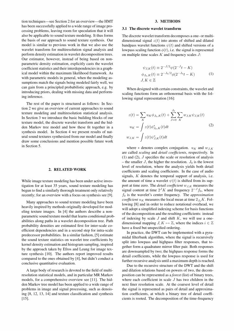
tion techniques—see Section 2 for an overview—the HMThas been successfully applied to a wide range of image pro-cessing problems, leaving room for speculation that it willalso be applicable to sound texture modeling. It thus formsthe basis of our approach to sound texture synthesis. Ourmodel is similar to previous work in that we also use thewavelet transform for multiresolution signal analysis andperform density estimation in wavelet decomposition trees.Our estimator, however, instead of being based on non-parametric density estimation, explicitly casts the waveletcoefficient statistics and their interdependencies in a graph-ical model within the maximum likelihood framework. Aswith parametric models in general, when the modeling as-sumptions match the signals being modeled fairly well, wecan gain from a principled probabilistic approach, e.g. byintroducing priors, dealing with missing data and perform-ing inference.

The rest of the paper is structured as follows: In Sec-tion 2 we give an overview of current approaches to soundtexture modeling and multiresolution statistical analysis.In Section 3 we introduce the basic building blocks of ourtexture model, the discrete wavelet transform and the hid-den Markov tree model and how these fit together in asynthesis model. In Section 4 we present results of nat-ural sound textures synthesized from our model and finallydraw some conclusions and mention possible future workin Section 5.

2. RELATED WORK

While image texture modeling has been under active inves-tigation for at least 35 years, sound texture modeling hasbegun to find a similarly thorough treatment only relativelyrecently; for an overview with a focus on synthesis see [9].

Many approaches to sound texture modeling have beenheavily inspired by methods originally developed for mod-eling texture images. In [4] the authors describe a non-parametric sound texture model that learns conditional prob-abilities along paths in a wavelet decomposition tree. Pathprobability densities are estimated first for inter-scale co-efficient dependencies and in a second step for intra-scalepredecessor probabilities. In a similar fashion, [5] estimatethe sound texture statistics on wavelet tree coefficients bykernel density estimation and histogram sampling, inspiredby the approach taken by Efros and Leung for image tex-ture synthesis [10]. The authors report improved resultscompared to the ones obtained by [4], but didn’t conduct aconclusive quantitative evaluation.

A large body of research is devoted to the field of multi-resolution statistical models, and in particular MR Markovmodels, for a comprehensive overview see [11]. The hid-den Markov tree model has been applied to a wide range ofproblems in image and signal processing, such as denois-ing [8, 12, 13, 14] and texture classification and synthesis[15].

3. METHODS

3.1 The discrete wavelet transform

The discrete wavelet transform decomposes a one- or multi-dimensional signal z(t) into atoms of shifted and dilatedbandpass wavelet functions ψ(t) and shifted versions of alowpass scaling function φ(t), i.e. the signal is representedon multiple time scales K and frequency scales J :

ψJ,K(t) ≡ 2−J/2ψ(2−J t−K)

φJ0,K(t) ≡ 2−J0/2φ(2−J0t−K)J,K ∈ Z

(1)

When designed with certain constraints, the wavelet andscaling functions form an orthonormal basis with the fol-lowing signal representation [16]:

z(t) =∑K

uKφJ0,K(t) +J0∑

J=0

∑K

wJ,KψJ,K(t)

uK =∫z(t)φ∗J0,K(t)dt

wJ,K =∫z(t)ψ∗J,K(t)dt

(2)

where ∗ denotes complex conjugation. uK and wJ,K

are called scaling and detail coefficients, respectively. In(1) and (2), J specifies the scale or resolution of analysis– the smaller J , the higher the resolution. J0 is the lowestlevel of resolution, where the analysis yields both detailcoefficients and scaling coefficients. In the case of audiosignals, K denotes the temporal support of analysis, i.e.the amount of time a wavelet ψ(t) is shifted from its sup-port at time zero. The detail coefficient wJ,K measures thesignal content at time 2JK and frequency 2−Jf0, wheref0 is the wavelet’s center frequency. The approximationcoefficient uK measures the local mean at time 2J0K. Fol-lowing [8] and in order to reduce notational overhead, wewill adopt a simplified indexing scheme for basis functionsof the decomposition and the resulting coefficients: insteadof indexing by scale J and shift K, we will use a one-dimensional mapping J,K 7→ Z, where the indices i ∈ Zhave a fixed but unspecified ordering.

In practice, the DWT can be implemented with a pyra-midal filterbank algorithm, where the signal is recursivelysplit into lowpass and highpass filter responses, that to-gether form a quadrature mirror filter pair. Both responsesare downsampled by two; the highpass response forms thedetail coefficients, while the lowpass response is used forfurther recursive analysis until a maximum depth is reached.

Due to the recursive structure of the DWT and the shiftand dilation relations based on powers of two, the decom-position can be represented as a forest (list) of binary trees,where each coefficient in scale J has two children in thenext finer resolution scale. At the coarsest level of detailthe signal is represented as pairs of detail and approxima-tion coefficients, at which a binary tree of detail coeffi-cients is rooted. The decomposition of the time-frequency

w1

w2

w3

w4

w5

w6

w7

w8

w9

w10

w11

w12

w13

w14

w15

u1Approximation

Detail 1

Detail 2

Detail 3

Detail 4

f

t

Tree 1 Tree 2

Figure 1: Four level wavelet time-frequency decomposition. Shown are two consecutive trees with frequency runningdownward and time to the right.

plane into multiple wavelet trees is shown graphically inFig. 1.

The recursive shifting and dilation performed by theDWT is also the reason for some desirable properties forthe analysis of natural sounds [8]: Locality, i.e. each band-pass atomψi is localized in both time and frequency, whichimplies multi-resolution, i.e. a nested set of scales in timeand frequency is analyzed and compression, i.e. the wave-let coefficient matrices of many real-world signals are near-ly sparse. These properties are desirable for the goal of es-timating the statistics of a wavelet decomposition, as willbecome evident in the next paragraph.

3.2 Hidden Markov Tree Models

In general, a hidden Markov model introduces hidden statevariables that are linked in a graphical model with Markovdependencies between the states, as is the case for the wide-ly used hidden Markov model (HMM). Often the hiddenstates can be viewed as encoding a hidden physical causethat is not directly observable in the signal itself or itstransformation in feature space.

In our research we focus on MR Markov processes thatare defined on pyramidally organized binary trees, in par-ticular the hidden Markov tree model. In this model, eachnode in a wavelet decomposition tree is identified with amixture model, i.e. a hidden, discrete valued state variablewith M possible values and an equal number of paramet-ric distributions (usually Gaussians) corresponding to theindividual values of the hidden state (Fig. 2).

Instead of assuming a Markov dependency on the wave-let coefficients as in parametric estimation methods (seeSection 2), the HMT model introduces a first order Markovdependency between a given hidden state and its children.In other words and for the example tree in Fig. 2, giventheir parent state variable s1, the subtrees rooted at the chil-dren s2 and s3 are conditionally independent. Similarly,since the wavelet coefficients are modeled by a distribu-

s1

s2

s3

s4

s5

s6

s7

s8

w4

w5

w6

w7

w3

w2

w1

w8

s9

w9

s10

w10

s11

w11

s12

w12

s13

w13

s14

w14

s15

w15

State variableWavelet coefficient

Figure 2: Hidden Markov tree model. Associated witheach wavelet coefficient at a certain position in the treestructure (black node) is a hidden state variable (whitenode), that indexes into a family of parametric distribu-tions.

tion that is only dependent on the node’s state, w2 and w3

are also independent of the rest of the tree given their par-ent state s1. Given enough data for parameter estimationand by increasing the number of states M , we can approx-imate the marginal distributions of wavelet coefficients toarbitrary precision. This allows us to model marginal dis-tributions that are highly non-Gaussian, but are Gaussianconditioned on the parent state variable.

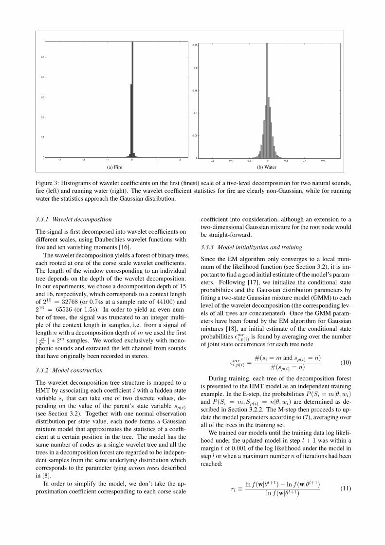
Even though the wavelet transform can be considereda de-correlator and the decomposition is sparse, the wave-let coefficients of real-world signals can not be consideredindependent, and there remain inter-coefficient dependen-cies that need to be taken into account in a statistical model.Fig. 3 shows histograms of wavelet coefficients for a par-ticular scale in natural sound signals. These distributions

are sharply peaked around zero with long symmetric tails,corresponding to the sparsity property of the wavelet trans-form: there’s a large number of small and only a few largecoefficients.

For modeling the non-Gaussian wavelet coefficient mar-ginal statistics, we use a two-state Gaussian mixture model,where one state encodes the peaked distribution of smallcoefficients and the other state encodes the tailed distribu-tion of high-valued coefficients. For wavelet coefficientsw = (w1, . . . , wN ) and hidden states s = (s1, . . . , sN ),the HMT is defined by the parameters

θ = {ps1(m), εmri,p(i), µi,m, σ

2i,m}

m, r ∈ {0, 1}, 1 ≤ i ≤ N(3)

with:

• ps1(m) = P (s1 = m), the probability of the rootnode s1 being in state m,

• εmri,p(i) = P (si = m|sp(i) = r), the conditional

probability of child si being in state m ∈ {0, 1}given the parent sp(i) is in state r ∈ {0, 1},

• µi,m, the mean of the wavelet coefficient wi given si

is in in state m (1 ≤ i ≤ N) and

• σ2i,m, the variance of the wavelet coefficientwi givensi is in state m (1 ≤ i ≤ N).

3.2.1 Training of the HMT

In order to find the best parameters fitting a given sourcesound, we update the model parameters θ given the train-ing data w = {wi} (a forest of binary wavelet trees, seeSection 3.1) using a maximum likelihood (ML) approach.The expectation maximization (EM) framework providesa solid foundation for estimating the model parameters θand the probabilities of the hidden states s and has beenformulated for wavelet-based HMM’s in [8]. The objec-tive function to be optimized is the log-likelihood functionln f(w|θ) of the wavelet coefficients given the parameters.The EM algorithm iteratively updates the parameters untilconverging to a local maximum of the log likelihood.

In the following we provide a schematic description ofthe algorithm. More information on how we initialized ourmodels and on the convergence criterion can be found inSection 3.3.

1. Initialization

(a) Select an initial model estimate θ0,

(b) Set iteration counter l = 0.

2. E step: Calculate P (s|w, θl), the probability of thehidden state variables S, yielding the expectation

Q(θ|θl) =∑

s∈{0,1}N

P (s|w, θl) ln f(w,s|θ). (4)

3. M step: Update parameters θ, in order to maximizeQ(θ|θl):

θl+1 = arg maxθQ(θ|θl). (5)

4. Convergence: Set l = l+1. If converged, then stop;else, return to E step.

3.2.2 E Step

The formulas for solving the hidden Markov tree E steppresented in [8] are susceptible to underflow due to themultiplication of a large number of probabilities smallerthan one. In [13] the authors develop an algorithm that isimmune to underflow and computes the probabilities p(si =m|w, θ) directly, instead of deriving them from p(si =m,w = w). The probabilities p(si = m, sρ(i) = n|w, θ),needed for computing the conditional state probabilities,can also be extracted directly from their algorithm. Similarto the original algorithm in [8], the above-mentioned prob-abilities are computed in separate upward and downwardrecursions, comparable to the computation of forward andbackward variables in conventional hidden markov mod-els. The algorithm has a slightly higher computationalcomplexity than the one in [8], although it is still linearin the number of observation trees. For a more thoroughtreatment of the computations involved see [13].

3.2.3 M Step

After having calculated P (s|w, θl) in the E step, the Mstep consists in straight-forward closed-form updates of theconditional state probabilities and the parameters of the ob-servation distributions.

First we calculate the probability of node i being in statem

psi(m) =1K

K∑k=1

P (ski = m|wk, θl) (6)

Then we update the model parameters by averaging overthe quantities computed in the E-step for each of the Ktraining examples:

εmri,p(i) =

∑Kk=1 P (sk

i = m, skp(i) = r|wk, θl)

Kpsp(i)(r)(7)

µi,m =∑K

k=1 wki p(s

ki = m|w, θl)

Kpsi(m)(8)

σ2i,m =

∑Kk=1(w

ki − µi,m)2P (sk

i = m|wk, θl)Kpsi(m)

(9)

3.3 Application to Sound Texture Synthesis

In this section we describe how the hidden Markov Treemodel is adapted to a sound texture synthesis application. 1

1 All of the algorithms used in this work were implemented in thefunctional programming language Haskell and a link for download-ing the package can be found at http://mtg.upf.edu/people/skersten?p=Sound%20Texture%20Modeling

!3 !2 !1 0 1 2

0

0.1

0.2

0.3

0.4

0.5

d5

(a) Fire!0.6 !0.4 !0.2 0 0.2 0.4 0.6

0

0.05

0.1

0.15

0.2

0.25

d1

(b) Water

Figure 3: Histograms of wavelet coefficients on the first (finest) scale of a five-level decomposition for two natural sounds,fire (left) and running water (right). The wavelet coefficient statistics for fire are clearly non-Gaussian, while for runningwater the statistics approach the Gaussian distribution.

3.3.1 Wavelet decomposition

The signal is first decomposed into wavelet coefficients ondifferent scales, using Daubechies wavelet functions withfive and ten vanishing moments [16].

The wavelet decomposition yields a forest of binary trees,each rooted at one of the corse scale wavelet coefficients.The length of the window corresponding to an individualtree depends on the depth of the wavelet decomposition.In our experiments, we chose a decomposition depth of 15and 16, respectively, which corresponds to a context lengthof 215 = 32768 (or 0.74s at a sample rate of 44100) and216 = 65536 (or 1.5s). In order to yield an even num-ber of trees, the signal was truncated to an integer multi-ple of the context length in samples, i.e. from a signal oflength n with a decomposition depth ofm we used the firstb n

2m c ∗ 2m samples. We worked exclusively with mono-phonic sounds and extracted the left channel from soundsthat have originally been recorded in stereo.

3.3.2 Model construction

The wavelet decomposition tree structure is mapped to aHMT by associating each coefficient i with a hidden statevariable si that can take one of two discrete values, de-pending on the value of the parent’s state variable sρ(i)

(see Section 3.2). Together with one normal observationdistribution per state value, each node forms a Gaussianmixture model that approximates the statistics of a coeffi-cient at a certain position in the tree. The model has thesame number of nodes as a single wavelet tree and all thetrees in a decomposition forest are regarded to be indepen-dent samples from the same underlying distribution whichcorresponds to the parameter tying across trees describedin [8].

In order to simplify the model, we don’t take the ap-proximation coefficient corresponding to each corse scale

coefficient into consideration, although an extension to atwo-dimensional Gaussian mixture for the root node wouldbe straight-forward.

3.3.3 Model initialization and training

Since the EM algorithm only converges to a local mini-mum of the likelihood function (see Section 3.2), it is im-portant to find a good initial estimate of the model’s param-eters. Following [17], we initialize the conditional stateprobabilities and the Gaussian distribution parameters byfitting a two-state Gaussian mixture model (GMM) to eachlevel of the wavelet decomposition (the corresponding lev-els of all trees are concatenated). Once the GMM param-eters have been found by the EM algorithm for Gaussianmixtures [18], an initial estimate of the conditional stateprobabilities εmr

i,p(i) is found by averaging over the numberof joint state occurrences for each tree node

εmri,p(i) =

#(si = m and sρ(i) = n)#(sρ(i) = n)

(10)

During training, each tree of the decomposition forestis presented to the HMT model as an independent trainingexample. In the E-step, the probabilities P (Si = m|θ, wi)and P (Si = m,Sρ(i) = n|θ, wi) are determined as de-scribed in Section 3.2.2. The M-step then proceeds to up-date the model parameters according to (7), averaging overall of the trees in the training set.

We trained our models until the training data log likeli-hood under the updated model in step l + 1 was within amargin t of 0.001 of the log likelihood under the model instep l or when a maximum number n of iterations had beenreached:

rl ≡ln f(w|θl+1)− ln f(w|θl+1)

ln f(w|θl+1)(11)

terminate when 0 ≤ t ≤ rl ∨ l ≥ n.

3.3.4 Synthesis

Sampling from the model begins by choosing an initialstate for the root of the tree based on the estimated prob-ability mass function (pmf) and sampling a wavelet coef-ficient from the gaussian probability distribution function(pdf) associated with the node and the sampled state. Thealgorithm proceeds by recursively sampling state pmfs andobservation pdfs at each node given the state of its imme-diate parent. After having sampled a number of trees fromthe model independently from each other—without any ex-plicit tree sequence model—the resulting forest of binarywavelet coefficient trees is transformed to the time domainby the inverse wavelet transform.

4. RESULTS

For a first qualitative evaluation we selected two texturalsounds, fire and running water, from a commercial collec-tion of environmental sound effects 2 .

Fig. 4 shows the spectrograms of the fire and the watersound, respectively (left column). The fire texture is com-posed of little micro-onsets stemming from explosions ofgas enclosed in the firewood. Inter-onset intervals are inthe range of a few milliseconds. The background is filledwith hisses, little pops and some low frequency noise. Thesound of a water stream on the other hand is characterizedby its overall frequency envelope with a broad peak below5 kHz and a narrow peak around 12 kHz, while the finestructure is not clearly discernible in the spectrogram.

Informally evaluating the synthesis results by listening 3

shows that the HMT model is able to capture key depen-dencies between wavelet coefficients of the textural sounds.In the case of fire, the model built from an analysis with thelonger wavelet function with ten vanishing moments is notable to reproduce the extremely sharp transients present inthe signal. All three fire reproductions capture the over-all perceptual quality of the original. This coherence isensured by the HMT model by capturing the across scalecoefficient dependencies. The temporal fine structure how-ever can deviate significantly from the original: In all threecases the onset patterns are denser than in the source soundand lack sequential coherence. This can be explained withthe fact that our model doesn’t capture temporal, i.e. within-scale dependencies of wavelet coefficients explicitly. Thismissing feature roughly corresponds to the autocorrelationfeature found to be important for the perception of texturesin both image and sound [15, 3].

Similar to the sounds of fire, the synthesis of the watersound shows an overall similar spectral shape to the origi-nal, although an important spectral peak is missing fromaround 12 kHz and the high frequency content is morenoisy in general (Fig. 4). In this sound, clearly noticeablebubbles form an important part of the temporal fine struc-ture, and this feature is missing from the synthesis. We

2 Blue Box SFX, http://www.eastwestsamples.com/details.php?cd index=36, accessed 2010-04-27.

3 The synthesis results of our experiments are available on theweb for reference, http://mtg.upf.edu/people/skersten?p=Sound%20Texture%20Modeling, accessed 2010-06-14

attribute this, as in the case of fire, to the missing autocor-relation feature in our synthesis model.

All of the synthesis examples show a repeating patternwith a length close to the wavelet tree size, i.e. directlyrelated to the decomposition depth, although there is someminor within-loop variation. This result is an indicationthat the model is overfitted to the source material and canbe explained with the relatively low number of training ex-amples per tree model (around 7 wavelet trees per 10 sec-onds of source material). We could alleviate the overfittingeffect in two ways: firstly, by using a significantly largertraining set, and secondly, by tying parameters of corre-lated wavelet coefficients and thereby reducing the numberof states and the number of mixture components. Simplytying parameters within one level of the wavelet decompo-sition however was found to be inadequate, because tem-poral fine structure gets lost and the synthesis result resem-bles a noisy excitation with roughly the spectral envelopeof the original.

In order to quantitatively assess the synthesis quality,we conducted a small listening experiment with eleven sub-jects. We selected three sound examples for each of the fivetexture classes applause, crowd chatter, fire, rain and run-ning water from the Freesound database 4 . We trimmedthe sounds to the first 20 seconds, selected the left chan-nel and downsampled this sound portion to a uniform sam-ple rate of 22.5kHz. We then trained a model for each ofthe sounds using a wavelet tree decomposition of a depthof 16, i.e. an analysis frame length of 1.5s, and stoppingtraining after 40 iterations. By sampling from the modelswe synthesized an eight second audio clip for each originalsound file and presented the examples in random order. Ina forced choice test, the subjects had to assign each syn-thesized sound to one of the five texture classes.

Table 1 shows the confusion matrix of the listening ex-periment and Table 2 lists the per-class accuracy. Appar-ently our model adequately captures the key perceptualproperties of the respective sound classes except in thecase of water and rain. The rain/water confusion can beexplained with the missing “larger-scale” fine structure inthe water examples (bubbling, whirling) that draws themcloser to the noisy nature of the synthesized rain. Whileapplause gets confused with rain on a surface because ofthe perceptual similarity between the micro-onsets that com-prise those texture sounds, the vocal quality of the crowdchatter is a clearly distinguishing feature, even if poorlysynthesized.

5. CONCLUSIONS

In this work we approached the problem of sound tex-ture synthesis by application of a multi-resolution statis-tical model. Our contribution is a model that is able tocapture key dependencies between wavelet coefficients forcertain classes of textural sounds. While the synthesis re-sults highlight some deficiencies that need to be addressedin future work, a parametric probabilistic approach to soundtexture modeling has important advantages:

4 http://freesound.org

Figure 4: Spectrograms of a fire sound (top left), its synthesis (top right) a water stream sound (bottom left) and its synthesis(bottom right). Both sounds were recorded at a sample rate of 44100 kHz. The spectrum analysis was performed with awindow size of 1024 and a hop size of 256.

Predictedapplause crowd fire rain water

Act

ual

applause 13 1 0 7 1crowd 0 24 1 5 2fire 0 0 30 0 3rain 1 1 2 17 12water 6 0 2 19 6

Table 1: Confusion matrix for the listening experiment’sresults with five sound classes of three examples each andeleven subjects. Due to an error during the model buildingprocess, the applause class contains only two examples.One user classification for the crowd class was not submit-ted.

Classapplause crowd fire rain water

Accuracy 0.59 0.75 0.91 0.52 0.18

Table 2: Class accuracies obtained in the listening experi-ment.

• Probabilistic priors can be used to deal with insuffi-cient training data or to expose expressive synthesiscontrol parameters.

• The model can be applied to inference tasks like clas-sification, segmentation and clustering.

When comparing the synthesized sounds to their origi-nal source sounds it becomes evident that the model fails tocapture some features that are crucial for auditory percep-tion of texture, most notably the intra-scale autocorrelationfeature. Another major limitation is the inadequate repre-sentation of infinite time series, because our model dividesthe signal into blocks of a size determined by the modeltree depth, thereby introducing artifacts caused by the po-sition of the signal relative to the beginning and the end ofthe block.

The most intuitive approach to overcome these limita-tions is to modify the graphical tree model itself, by allow-ing additional conditional dependencies between nodes onthe same hierarchy level. Because graphs that satisfy cer-tain conditions on their structure, and in particular on thecycles formed by their edges, still allow for efficient pa-rameter estimation in the EM framework—see [19] for athorough treatment—it is possible to model within-scalecoefficient dependencies without resorting to Markov-chainMonte-Carlo or other simulation methods. The significantincrease in the number of parameters needs to be addressedby aggressive tying, i.e. by using the same parameters for

a set of variables in the model that exhibit the same statis-tics. While tying within tree levels yields unsatisfactoryresults for the model described in this paper, a modifiedmodel might be able to capture just enough temporal cor-relations to make this tying scheme feasible. By explicitlymodeling dependencies across time, the wavelet decompo-sition depth wouldn’t be the only way to capture temporalcontext any longer and could be decreased significantly,resulting in a vastly reduced set of parameters.

6. ACKNOWLEDGMENTS

Many thanks to Jordi Janer, Ferdinand Fuhrmann and theanonymous reviewers for their valuable suggestions and tothose who kindly participated in our listening test. Thiswork was partially supported by the ITEA2 Metaverse1Project 5 . The first author is supported by the FI-DGR2010 scholarship of the Generalitat de Catalunya, the sec-ond author holds a Juan de la Cierva scholarship of theSpanish Ministry of Science and Innovation.

7. REFERENCES

[1] R. M. Schafer, The Soundscape: Our Sonic Environ-ment and the Tuning of the World. Destiny Books,1994.

[2] N. Saint-Arnaud, Classification of Sound Textures.Master thesis, Massachusetts Institute of Technology,1995.

[3] J. H. McDermott, A. J. Oxenham, and E. P. Simon-celli, “Sound texture synthesis via filter statistics,” inProceedings IEEE Workshop on Applications of SignalProcessing to Audio and Acoustics, (New Paltz, NY),Oct. 2009.

[4] S. Dubnov, Z. Bar-Joseph, R. El-Yaniv, D. Lischinski,and M. Werman, “Synthesizing sound textures throughwavelet tree learning,” Computer Graphics and Appli-cations, IEEE, vol. 22, pp. 38–48, July 2002.

[5] D. ORegan and A. Kokaram, “Multi-Resolution soundtexture synthesis using the Dual-Tree complex wavelettransform,” in Proc. 2007 European Signal ProcessingConference (EUSIPCO), 2007.

[6] A. Kokaram and D. O’Regan, “Wavelet based high res-olution sound texture synthesis,” in Proc. 31st Interna-tional Conference: New Directions in High ResolutionAudio, June 2007.

[7] D. D. Po and M. N. Do, “Directional multiscale mod-eling of images using the contourlet transform,” IEEETransactions on Image Processing, vol. 15, no. 6,p. 16101620, 2006.

[8] M. Crouse, R. Nowak, and R. Baraniuk, “Wavelet-based statistical signal processing using hidden markovmodels,” Signal Processing, IEEE Transactions on,vol. 46, no. 4, pp. 886–902, 1998.

5 http://www.metaverse1.org

[9] G. Strobl, G. Eckel, D. Rocchesso, and S. le Grazie,“Sound texture modeling: A survey,” 2006.

[10] A. A. Efros and T. K. Leung, “Texture synthesis byNon-Parametric sampling,” in Proceedings of the In-ternational Conference on Computer Vision-Volume 2- Volume 2, p. 1033, IEEE Computer Society, 1999.

[11] A. Willsky, “Multiresolution markov models for sig-nal and image processing,” Proceedings of the IEEE,vol. 90, no. 8, pp. 1396–1458, 2002.

[12] H. Choi, J. Romberg, R. Baraniuk, and N. Kingsbury,“Hidden markov tree modeling of complex wavelettransforms,” in Acoustics, Speech, and Signal Process-ing, 2000. ICASSP ’00. Proceedings. 2000 IEEE In-ternational Conference on, vol. 1, pp. 133–136 vol.1,2000.

[13] J. Durand, P. Goncalves, and Y. Guedon, “Computa-tional methods for hidden markov tree models-an ap-plication to wavelet trees,” Signal Processing, IEEETransactions on, vol. 52, no. 9, pp. 2551–2560, 2004.

[14] D. H. Milone, L. E. D. Persia, and M. E. Torres, “De-noising and recognition using hidden markov mod-els with observation distributions modeled by hid-den markov trees,” Pattern Recogn., vol. 43, no. 4,pp. 1577–1589, 2010.

[15] G. Fan and X. G. Xia, “Wavelet-based texture analy-sis and synthesis using hidden markov models,” IEEETransactions on Circuits and Systems I: FundamentalTheory and Applications, vol. 50, no. 1, p. 106120,2003.

[16] I. Daubechies, “Orthonormal bases of compactly sup-ported wavelets,” Communications on Pure and Ap-plied Mathematics, vol. 41, no. 7, pp. 909–996, 1988.

[17] G. Fan and X. G. Xia, “Improved hidden markovmodels in the wavelet-domain,” IEEE TRANS SIGNALPROCESS, vol. 49, no. 1, p. 115120, 2001.

[18] C. M. Bishop, Pattern Recognition and MachineLearning. Information Science and Statistics, NewYork, NY, USA: Springer, 2006.

[19] H. Lucke, “Which stochastic models allow Baum-Welch training?,” Signal Processing, IEEE Transac-tions on, vol. 44, no. 11, pp. 2746–2756, 1996.