13th World Conference on Earthquake Engineering Vancouver, B.C., Canada

August 1-6, 2004 Paper No. 1572

SOURCE CHARACTERIZATION OF MEXICAN SUBDUCTION EARTHQUAKES FOR THE PREDICTION OF STRONG GOUND

MOTIONS

Jorge AGUIRRE1 and Kojiro Irikura2

SUMMARY The empirical Green’s function method allows to simulate records of big earthquakes using records of small ones. The great advantage of this method is that the information of the path and site effects are included in the small records which allows to simplify the calculations in the absence of nonlinear effects at the sites. However to carry out simulations of future earthquakes it is necessary to construct source model consisting on the outer parameters (i.e. focal mechanism, total area of rupture) and the inner ones (size, number and position of the roughness). This study uses data of Mexican subduction earthquakes with the objective of proving the different relationships presented previously, with the objective of validating them or in its case to propose some other of regional validity. Using records of the Guerrero Accelerograph Array from earthquakes occurring during the last 15 years we found that the relationships proposed by Dan et al. (2001) works appropiately for the Mexican subduction earthquakes. We also found that the fault areas obtained with data of this regional array, gave a good estimation of the size of the biggest asperity. These sizes are well predicted by the relationship for subduction earthquakes given by Somerville et al. (2002).

INTRODUCTION The evaluation of the seismic risk has become a topic of relevance especially in countries that have great seismic activity. With that purpose many methods have been developed that focus on the evaluation of the risk from different perspectives. One of these focuses is the called seismic scenario that consists of carrying out the evaluation of the risk being based on simulations of

1 Instituto de Ingeniería, Universidad Nacional Autónoma de México. Ciudad Universitaria. Apartado postal 70-472, Coyoacán, 04510 México D.F 2 Disaster Prevention Research Institute, Kyoto University. Gokasho, Uji, Kyoto 611-0011, Japan..

seismic movements of well-known active faults that constitute a potential seismic source in the near future. Inside this focus several methods are used for the simulation of the movements generated by the potential seismic source. The methods based on simulating the propagation by means of finite elements or finite differences are commonly used for this purpose. Although the computation capacity no longer constitutes an obstacle for these techniques, the distribution of S and P wave velocities in the different strata in one, two or three dimensions are not known accurately enough as to carry out simulations to high frequencies. Another method that allows the evaluation of seismic motions is the empirical Green’s function method. It has the great advantage of being able to reach frequencies beyond 10 Hz in the simulations. Recently, some seismologists have been carrying out several studies to understand the relationships between some inner and outer parameters in order to be able to make more accurate predictions of strong motions for future earthquakes. They have been studying those parameters that are responsible for the generation of strong motions especially. These relationships in general, and for each region in particular, allows to carry out evaluation of the seismic hazard following a series of steps first proposed by Irikura (2002) like recipe to estimate the strong movements of earthquakes taken place in active faults. A lot of work has been done in the case of inland earthquakes. Somerville et al. (1999), using results of many kinematic inversions obtained some relationships that synthesize the main characteristics of the earthquakes. Especially they are focused in those that are the main strong ground motions generators. It was found that the area of the asperities represented 22% of the total rupture area. Likewise they presented the relationships between the seismic moment and the rupture area, the slip average, the combined area of asperities, the area of the biggest asperity, among others. These relationships are of great utility for the prediction of seismic movements limiting the values that can be considered in particular for the simulation of an active fault. The same relationships for subduction earthquakes with inverse focal mechanism have been obtained, although they are not equally convincing. It is needed to continue collecting data for the earthquakes of this type which occurred in subduction areas. Somerville et al. (2002) using heterogeneous rupture slip models of big subduction earthquakes, studied the scale relationships systematically with the seismic moment, and they compared them with those obtained for inland earthquakes. They found that the main differences between the models of subduction slip and inland earthquakes were in the total rupture area. They concluded that the areas of the subduction earthquakes were, on the average, two to three times larger that those of the inland earthquakes having the same seismic moment. Consequently this produced smaller stress drops for the subduccion earthquakes than the inland ones. On the other hand, Dan et al. (2001), studied the quantity of effective stress and slip taken place in an asperity and in the rest of the rupture area based on models of rupture of variable slip and their relationship with the flat levels of acceleration spectra. The present study uses data of some Mexican subduction earthquakes with the objective of proving the different relationships presented previously, with the objective of validating them or

in its case to propose some other one of regional validity.

DATA This section has the purpose of validating the relationship proposed by Dan et al. (2001) among the plane level of acceleration in high frequencies and the seismic moment. The relationship proposed by Dan et al. (2001) is

3

1

017

21046.2][ xMx

s

cmdinaA =−

(1),

where A it is the flat level of the source acceleration spectrum and 0M is the seismic

moment.

In order to find these spectra based on observed data we considered the stations Atoyac (ATYC), Coyuca (COYC), Filo de Caballo (FIC2), Los Magueyes (MAGY), Ocotillo (OCLL), San Marcos (SMR2), Súchil (SUCH), Tonalapa (TNLP), and Zihuatanejo (AZIH), that according to Humphrey and Anderson (1994), present a flat site response in the band from 0.3 to 30 Hz. All these stations belong to the Guerrero Accelerographic Array. The selected earthquakes were recorded in some of the above mentioned stations, and all of them had reverse focal mechanism (reported by Harvard-CMT in the period from the January 1st of 1990 to December 31st of 1999). The epicenters were located between 15 and 20 degrees latitude, and -107 and -95 degrees of longitude. Additionally, five very well-known earthquakes September 19th of 1985 (09-19-85), February 8th of 1988, March 10th of 1989, April 25th of 1989, and May 2nd 1989; were included. In total 31 earthquakes were considered, 24 of them registered in two or more stations. The epicentres of the considered earthquakes appear in the Figure 1.

Figure 1. Epicentral localization of the 32 earthquakes used in this study.

FLAT LEVEL OF ACCELERATION SPECTRA The acceleration records of the horizontal components were corrected as is indicated by the following equation:

βπ

πρβ )(30 85.0

4*)( fQ

fR

eR

fAA = (2),

where 66.0273)( ffQ = (3),

R is the hipocentral distance, β is the S wave velocity (here considered as 3.61 km/s like in Humphrey and Anderson (1994) and Valdez et al. (1986) appropriate for the region), ρ is the

density (2.83 3/ cmg ), the constant 0.85 is used to consider the average S waves radiation pattern and the partition of the energy in two horizontal components. The equation (3) is taken from Ordaz and Singh (1992). The epicentral distances have been calculated with the hipocentral localizations of the Instituto of Ingeniería (I. de I.) and of the Servicio Sismológico National (SSN), except for the earthquakes of 09-19-85 and 10-09-95 whose hipocentral localizations were taken of the Harvard CMT. Some examples of the spectra already corrected of the 31 earthquakes appear in the Figures 2.

Figure 2. Spectra of acceleration corrected for the earthquakes of the 04-25-89 (left side) and 10-24-93 (right side). The component EW is in the upper part and the NS in the bottom

To characterize the flat level of frequency in the acceleration spectra we proceeded as follows. First, based on the graphs of the spectra for all the 31 earthquakes (as those in Figure 2), we determined the band width for the frequencies inside which the flat levels would be estimated. Taking into account that band width, the flat level was obtained for each spectrum averaging the spectral amplitudes logarithmically in that interval. For each event with records in more than one station it was obtained the logarithmic average and the standard deviations of the flat levels. This procedure is exemplified for the case of the earthquake of the 09-19-85 in the Figure 3. In these graphs the horizontal lines show: the average flat level and their standard deviations in the band width where they were calculated. Table 1 shows the dates of the used earthquakes, the stations that recorded them, the seismic moment, the epicentral localizations, as well as the used ranges of frequency and the values of the flat levels. Note that the Harvard CMT's epicentral localizations as well as the epicentral locations determined from the local array data (I. de I. and SSN) are also shown.

Figure 3. Example of the determination of levels planes their averages and standard deviations for the case of the earthquake of 09-19-85, the NS component is in top and EW component in bottom, the horizontal lines show: the level plane average and their logarithmic deviations standard in the interval where they are calculated.

TABLE 1

• These values were calculated using the distance calculated with Harvard CMT'S epicentral localization.

DATE Stations Moment

[dyne-cm] CMT Epicenter

(IdeI SSN) CMT Depth (IdeI SSN)

Frequency Range for Flat

(ew)

][2s

cmdyne −

(ns)

][2s

cmdyne −

1985/09/19 ATYC COYC FIC2

SUCH 1.10e+28

17.91,101.99 (18.081,102.942)

21.3 (15)

0.63-7.59 1.37697e+27 * 3.27458e+27

1.47918e+27 * 3.45341e+27

1988/02/08 ATYC COYC MAGY

SUCH TNLP 7.37e+24

17.03,100.35 (17.494,101.157)

47.8 (19)

2.29-15.14 9.98472e+25 9.89133e+25

1989/04/25 ATYC COYC FIC2

OCLL SMR2 2.39e+26

16.83,99.12 (16.603,99.400)

15.0 (19)

0.52-8.71 1.0641e+26 1.08935e+26

1989/05/02 COYC FIC2 OCLL

SMR2 1.91e+24

16.82,99.35 (16.637,99.513)

47.9 (13)

1.00-10.00 3.01895e+25 2.94489e+25

1989/03/10 ATYC MAGY SUCH

TNLP 1.35e+24

16.91,100.44 (17.446,101.089)

46.8 (18)

1.90-15.85 2.54377e+25 2.55001e+25

1990/01/13 FIC2 OCLL SMR2

TNLP 1.00e+24

16.33,99.67 (16.820,99.629)

34.2 (12)

2.75-12.02 2.39457e+25 2.40409e+25

1990/05/11 ATYC FIC2 MAGY

SUCH 2.48e+24

17.24,100.56 (17.134,100.304)

15.0 (18)

1.15-9.12 1.49803e+25 1.51555e+25

1990/05/31 ATYC AZIH FIC2

MAGY SUCH 7.49e+24

16.77,100.12 (17.106,100.893)

26.0 (16)

0.91-8.32 4.51428e+25 4.31058e+25

1991/01/14 AZIH FIC2 TNLP 1.89e+24 18.39,101.37

(17.838,101.854) 67.8 (25)

1.66-9.12 5.61566e+25 5.53798e+25

1991/04/01 TNLP 6.25e+24 16.70,97.68

(16.044,98.387) 39.8 (26)

1.20-10.00 0.74365e+26 0.78978e+26

1992/02/12 AZIH 7.03e+23 17.78,101.14

(17.733,101.058) 33.9 (<5)

0.91-22.91 0.17764e+26 0.12840e+26

1992/03/31 ATYC FIC2 MAGY

TNLP 1.55e+24

16.99,100.65 (17.233,101.302)

15.0 (11)

1.15-13.18 3.49965e+25 3.81667e+25

1992/04/01 AZIH TNLP 7.33e+23 17.10,100.51

(17.333,101.266) 60.0 (18)

2.51-10.00 2.52916e+25 2.46588e+25

1992/06/07 TNLP 1.19e+24 16.40,98.28

(16.222,98.870) 15.4 (5)

0.76-7.60 0.25466e+26 0.24343e+26

1993/03/31 ATYC FIC2 MAGY

TNLP 1.95e+24

17.29,100.89 (17.180,101.020)

26.2 (8)

0.72-18.20 2.21248e+25 2.10620e+25

1993/05/15 COYC SMR2 TNLP 1.41e+25 16.45,97.92

(16.430,98.740) 38.5 (20)

1.00-8.71 8.80735e+25 1.07528e+26

1993/10/24 ATYC COYC FIC2 OCLL SMR2 TNLP

1.01e+26 16.77,98.61

(16.54,98.98) 21.8 (19)

0.69-10.00 1.18195e+26 1.261195e+26

1995/04/27 AZIH 7.29e+23 18.04,101.66

(17.880,101.64) 41.6 (61)

1.00-10.00 0.24292e+26 0.23018e+26

1995/09/14 ATYC COYC OCLL

TNLP 1.31e+27

16.73,98.54 (16.31,98.88)

21.8 (22)

0.51-8.32 1.96679e+26 2.17228e+26

1995/10/09 TNLP 1.15e+28 19.34,104.80

(18.74,104.67) 15.0 (5)

0.275-1.74 0.12812e+28 * 0.11331e+28

0.13424e+28 * 0.11872e+28

1996/02/25 TNLP 5.51e+26 15.88,97.98

(15.83,98.25) 15.0 (3)

0.07-1.99 0.66472e+26 0.64340e+26

1996/03/13 SMR2 TNLP 6.37e+23 16.93,98.86

(16.52,99.08) 29.4 (18)

1.20-12.00 2.98936e+25 2.70708e+25

1996/04/23 ATYC AZIH 2.42e+24 17.13,101.84

(17.11,101.60) 36.8 (17)

0.66-13.18 1.90404e+25 1.78913e+25

1996/07/15 ATYC AZIH OCLL

TNLP 9.95e+25

17.50,101.12 (17.45,101.16)

22.4 (20)

1.00-10.00 1.15609e+26 1.16396e+26

1996/07/18 ATYC AZIH TNLP 1.59e+24 17.35,101.02

(17.54,101.20) 26.2 (20)

1.10-12.02 3.34649e+25 2.97328e+25

1997/01/21 SMR2 2.09e+24 16.49,97.99

(16.44,98.15) 39.7 (18)

1.00-8.32 0.25734e+26 0.36306e+26

1998/05/09 ATYC AZIH COYC

SUCH 8.44e+23

17.31,101.00 (17.34,101.41)

36.2 (18)

2.00-13.80 2.69882e+25 2.73504e+25

1998/05/16 ATYC SUCH 6.85e+23 17.56,101.54

(17.25,101.35) 33.0 (14)

1.00-7.94 1.39468e+25 1.55086e+25

1998/07/05 ATYC COYC OCLL

SMR2 TNLP 1.07e+24

16.92,99.73 (16.83,100.12)

37.6 (5)

1.90-13.18 1.56746e+25 1.43779e+25

1998/07/11 ATYC SUCH TNLP 1.83e+24 17.28,101.17

(17.25,101.54) 24.1 (5)

0.72-11.50 2.81928e+25 3.03071e+25

1998/07/12 ATYC COYC OCLL

SUCH TNLP 1.93e+24

16.78,99.91 (16.83,100.44)

15.0 (4)

0.9-8.3 1.19396e+25 1.13429e+25

Figure 4. Relationship between the flat level of acceleration spectrum and the seismic moment of Mexican subduction earthquakes. The points represent individual events, the line is the relationship proposed by Dan et al. (2001), for subduction earthquakes. Here the results are shown for the component EW.

Figure 5. Relationship between the flat level acceleration spectrum and the seismic moment of Mexican subduction earthquakes. The points represent individual events, the line is the relationship proposed by Dan et al. (2001), for subduction earthquakes. Here the results are shown for the component NS.

The averages of the flat levels of the acceleration spectra were obtained independently for each component. In the Figures 4 and 5 the graphs of the averages of these plane levels are shown versus seismic moment as well as the standard deviation when it has been calculated for the component EW and NS respectively. The straight line that appears in the Figures is calculated with the equation (1) proposed by Dan et al. (2001). We can observe that the relationship proposed by Dan et al. (2001) predicts the flat levels of acceleration appropriately for the Mexican subduction earthquakes. The Michoacán earthquake of 09-19-85 is included in the earthquakes reported by Dan et al. (2001) with a flat level smaller than the values obtained in this study for both components. The difference resides in the way that Dan et al. (2001) use to determine it. They extrapolated the low frequency spectra based on heterogeneous slip displacements from kinematic inversions. They did not use any records as is the case in the present study. RELATIONSHIP BETWEEN THE AREA OF THE BIGGEST ASPERITY AND THE SEISMIC

MOMENT FOR MEXICAN EARTHQUAKES. To examine the relationship among the area of the larger asperity and the seismic moment lets consider the results shown by Humphrey and Anderson (1994). They obtained the source spectrum of 82 earthquakes after removing the site and path effects. We selected 8 earthquakes from those, with reverse focal mechanism. We took the radius of the source that they obtained using the average corner frequency and the relationship by Brune (1970):

cc f

rπ

β2

34.2= (4).

With the radii we calculate the equivalent area and then ploted it against the seismic moment, in Figure 6. In the same Figure the relationship proposed by Somerville et al. (2002) between the seismic Moment and the area of the large asperity for subduction earthquakes is plotted. That relationship is

3/20

1621 104)( xMxCkmA −= (5),

where 0M is the seismic moment in dyne-cm, and C4 for subduction earthquakes takes the

value of 8.87. In Figure 6 it can be observed that the predicted area based on the relationship fits appropriately the area that is considered as the source area in Humphrey and Anderson. Considering that the data used by Humphrey and Anderson are acceleration records it is probable that indeed the estimates that they carried out are on the area of the largest asperity instead of the total area of the source. Using our data set, we also estimated the seismic moment and corner frequencies for all the 31 earthquakes from the displacement spectra (after integrating the corrected acceleration spectra). In Figure 7, we ploted the estimated areas versus the seismic moment, resulting from our corner frequencies in the equation 4.

Figure 6. Relationship between the area of the large asperity and the seismic moment. The points represent the area of the source reported by Humphrey and Anderson (1994). The line represents the relationship reported by Somerville et al. (2002) for subduction earthquakes.

Figure 7. Relationship between the area of the large asperity and the seismic moment. The points represent the area of the source obtained in the present study. The line represents the relationship reported by Somerville et al. (2002) for subduction earthquakes. The three graphs, in Figures 6 and 7, show the same tendency. For one side this allows us to validate the relationship of Somerville et al. (2002) for the Mexican subduction earthquakes, especially for those that have moments larger than 24102x dyne-cm, for those that the relationship seems to work better. From the Figure 6, the area of the largest asperity seems to be overestimated by the Somerville et al. (2002) relationship for seismic moments smaller than

24102x dyne-cm. On the other hand if we consider the seismic moments obtained with the

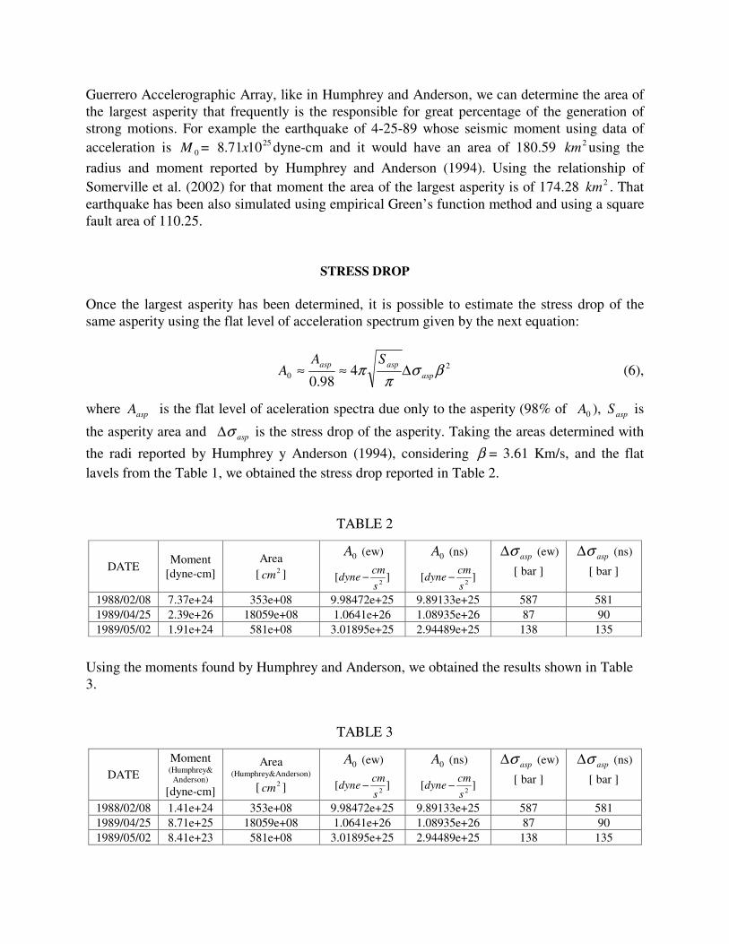
Guerrero Accelerographic Array, like in Humphrey and Anderson, we can determine the area of the largest asperity that frequently is the responsible for great percentage of the generation of strong motions. For example the earthquake of 4-25-89 whose seismic moment using data of acceleration is 0M = 251071.8 x dyne-cm and it would have an area of 180.59 2km using the

radius and moment reported by Humphrey and Anderson (1994). Using the relationship of Somerville et al. (2002) for that moment the area of the largest asperity is of 174.28 2km . That earthquake has been also simulated using empirical Green’s function method and using a square fault area of 110.25.

STRESS DROP Once the largest asperity has been determined, it is possible to estimate the stress drop of the same asperity using the flat level of acceleration spectrum given by the next equation:

20 4

98.0βσ

ππ asp

aspasp SAA ∆≈≈ (6),

where aspA is the flat level of aceleration spectra due only to the asperity (98% of 0A ), aspS is

the asperity area and aspσ∆ is the stress drop of the asperity. Taking the areas determined with

the radi reported by Humphrey y Anderson (1994), considering β = 3.61 Km/s, and the flat lavels from the Table 1, we obtained the stress drop reported in Table 2.

TABLE 2

DATE Moment

[dyne-cm] Area

[ 2cm ]

0A (ew)

][2s

cmdyne −

0A (ns)

][2s

cmdyne −

aspσ∆ (ew)

[ bar ] aspσ∆ (ns)

[ bar ]

1988/02/08 7.37e+24 353e+08 9.98472e+25 9.89133e+25 587 581 1989/04/25 2.39e+26 18059e+08 1.0641e+26 1.08935e+26 87 90 1989/05/02 1.91e+24 581e+08 3.01895e+25 2.94489e+25 138 135

Using the moments found by Humphrey and Anderson, we obtained the results shown in Table 3.

TABLE 3

DATE Moment (Humphrey&

Anderson)

[dyne-cm]

Area (Humphrey&Anderson)

[ 2cm ]

0A (ew)

][2s

cmdyne −

0A (ns)

][2s

cmdyne −

aspσ∆ (ew)

[ bar ] aspσ∆ (ns)

[ bar ]

1988/02/08 1.41e+24 353e+08 9.98472e+25 9.89133e+25 587 581 1989/04/25 8.71e+25 18059e+08 1.0641e+26 1.08935e+26 87 90 1989/05/02 8.41e+23 581e+08 3.01895e+25 2.94489e+25 138 135

Now, if we consider the areas given by the relation in Somerville et al. (2002) for subduction earthquakes (equation 5), we obtained the results shown in Table 4.

TABLE 4

DATE Moment (Humphrey&

Anderson)

[dyne-cm]

Area (Somerville et al (2002))

[ 2cm ]

0A (ew)

][2s

cmdyne −

0A (ns)

][2s

cmdyne −

aspσ∆ (ew)

[ bar ] aspσ∆ (ns)

[ bar ]

1988/02/08 1.41e+24 1117e+08 9.98472e+25 9.89133e+25 330 327 1989/04/25 8.71e+25 17428e+08 1.0641e+26 1.08935e+26 89 91 1989/05/02 8.41e+23 821e+08 3.01895e+25 2.94489e+25 116 113

If we consider the areas given by the relationship in Somerville et al. (2002) for subduction earthquakes (equation 5) and the flat level of acceleration spectra given by the relationship in Dan et al. (2001) in equation 1, we always get an stress drop of aspσ∆ = 91 bars. Using data

from the Guerrero Acelerographic Array Ordaz et al. (1995) found stress drop of 150 and 200 bars for the 1998/04/25 and 1998/05/02 earthquakes respectively. In Humphrey and Anderson (1994) the stress drop reported for the three earthquakes are 525, 89, and155 (for 1988/02/08, 1989/04/25, and 1989/05/02 earthquakes respectively).

THE FLAT LEVEL OF ACCELERATION SPECTRA FOR TOKACHI-OKI, JAPAN EARTHQUAKE OF SEPTEMBER 26, 2004 AND AFTERSHOCKS

On September 26 2003, the Tokachi-oki earthquake (Mw = 7.9) occurred off Tokachi, Hokkaido Island, Norhern Japan. Two people were missing and more than 800 people were injured. In this region the Pacific plate subducts toward N60 o W beneath the Hokkaido region (Yagi, 2004). In this fault zone large interplate earthquakes occurred in 1952 (Ms 8.2), 1958 (Ms 8.1), 1969 ( Ms 7.8), and 1975 (Ms 7.4). We used the records of 17 events recorded in the 29 stations. The epicenter locations of the events used in this study were plotted in Figure 8. The moment magnitude of the earthquakes ranging form Mw = 4.7 to Mw = 7.9, been the largest one the magnitude of the mainshock of the Tokachi-oki earthquake. Most of the events are aftershocks of Tokachi-oki earthquake. We corrected the data using the corrections of the equation (2) using the following value for the quality factor

0.13.83)( ffQ = (7) obtained by Yamamoto et al. (1995). That value is similar to the one obtained by Morikawa and Sasatani (2000) that is 0.19.120)( ffQ = . Even though the stations are in borehole at depths

more than 100 m and can be regarded as rock sites; we believe that the destructive interference of the reflected waves can affect the flat level of acceleration spectra. Then we obtained and corrected the site effect.

Figure 8. Location of the KiK-net stations (left site) and epicentral localization of the earthquakes used in this study for the Tokachi-oki earthquake, Hokkaido, Japan.

Figure 9. Relationship between the flat level acceleration spectrum and the seismic moment for Tokachi-oki earthquake (green dot), after shocks, and other subduction earthquakes occurred in 2003. The points represent individual events, the line is the relationship proposed by Dan et al. (2001), for subduction earthquakes. Here the results are shown for the component EW.

This earthquake was recorded in many stations of the KiK-net. The KiK-net had instruments at borehole and surface sites. We selected borehole acceleration records from 29 KiK-net stations for this study. The stations are located at depths more than 100 m and their locations are shown in Figure 8. The averages of the flat levels of the acceleration spectra are plotted in the Figures 9 and 10 versus seismic moment as well as the standard deviation for the component EW and NS. The straight line that appears in the figures is calculated with the equation (1) proposed by Dan et al. (2001).

Figure 10. Relationship between the flat level acceleration spectrum and the seismic moment for Tokachi-oki earthquake (green dot), after shocks, and other subduction earthquakes occurred in 2003. The points represent individual events, the line is the relationship proposed by Dan et al. (2001), for subduction earthquakes. Here the results are shown for the component NS.

DISCUSION AND CONCLUSIONS In the present study, acceleration records of Mexican subduction earthquakes were used to validating previously obtained scaling relationships and to propose some other relationships for regional validity. Using records of the Guerrero Accelerograph Array from earthquakes occurring during the last 15 years we found that the relationships proposed by Dan et al. (2001) for estimating the flat level of acceleration spectra works appropriately for the Mexican subduction earthquakes. The largest earthquake that we consider (09-19-85), shows a higher level than the value that Dan et al. (2001) relationship predicts. We also found that the fault areas obtained with data of this regional array, gave a good estimation of the size of the biggest asperity. These sizes were well predicted by the relationship for subduction earthquakes given by Somerville et al. (2002).

Also we used a set of 19 earthquakes recorded in 29 borehole stations that occurred during 2003 close to Hokaido Island in the north of Japan. After correcting the data for path and site effect the high frequency level of acceleration spectra was determined. The results showed an alignment parallel to the Dan et al. (2001) relationship for those earthquakes with a moment smaller than 26101x dyne-cm but systematically within larger values. There are two earthquakes that have large acceleration level that departs substantially from the general tendency. One of them, the May 5, 2003 Miyagiken-oki earthquake exhibits the largest acceleration level. The flat level of acceleration spectra of this earthquake has been obtained by Satoh (2004). She concluded that this earthquake has a higher level than the Dan et al. (2001) relationship. So this earthquake is a special case. The other earthquake that showed large flat acceleration spectra is the July 27, 2003 earthquake occurring in the northern part of the Japan Sea with a depth of about 500 km. These kinds of earthquakes exhibit an anomalous intensity pattern. Furumura (2003) suggested that for these deep earthquakes the waves were traveling as guided waves through the plate producing larger intensities in places far from the epicenter and smaller intensities in places closer to the epicenter. Then it is possible that this mechanism produces the high flat level of acceleration that we obtained. So these two earthquakes should be discussed separately. Finally, the acceleration spectra for the 2003 Tokachi-oki earthquake obtained in this study shows a higher flat level than the expected based on the Dan et al. (2001) relationship.

ACKNOLEDGMENTS This work has been done during the visits of the first author to DPRI, Kyoto University in 2003 and 2004. The Mexican waveform data used was obtained from the “Base Nacional de Datos de Sismos Fuertes”. The Japanese waveform data used was provided by the KiK-net, which belong to the National Research Institute for Earth Science and Disaster Prevention (NIED). Most of the graphs shown in this article were done using Generic Mapping Tools (Wessel and Smith, 1998). Part of data processing was done using SAC2000 (Goldstein et al., 1999).

REFERENCES 1. Brune, J.N. (1970), “Tectonic stress and the spectra of seismic shear waves from earthquakes”, J. Geophys. Res., 75, 4997-5009.

2. Dan, K., M. Watanabe, T. Sato and T. Ishii (2001),”Short-Period Source Spectra Inferred from Variable-Slip Rupture Models and Modeling of Earthquake Faults for Strong Motion Prediction by Semi-empirical Method”, J. Struct. Constr. Eng., AIJ, No. 545, 51-62. (in Japanese).

3. Furumura, T. (2003). “Large Scale Parallel 3D Simulation of Regional Wave Propagation Using the Earth Simulator”, Eos Trans. AGU, 84(46), Fall Meet. Suppl., Abstract S42J-02.

4. Goldstein, P., D. Dodge, and M. Firpo (1999). SAC2000: Signal processing and analysis tools for seismologists and engineers, UCRL-JC_135963, invited contribution to the IASPEI International Handbook of Earthquake and Engineering Seismology.

5.Humphrey, J. R. Jr and J. Anderson (1994). “Seismic Source Parameters from the Guerrero Subduction Zone”, Bull. Seism. Soc. Am., 84, 1754-1769.

6. Morikawa, N., and T. Sasatani (2000), “The 1994 Hokkaido Toho-oki earthquake sequence: the complex activity of intra-slab and plate boundary earthquakes”, Phys. Earth Planet Inter, 121, 39-58. 7.Ordaz, M., J. Arboleda, and S. K. Singh (1995). “A scheme of random summation o an empirical Green’s function to estimate ground motions from future large earthquakes”, Bull. Seism. Soc. Am., 85, 1635-1647. 8. Satoh, T. (2004), “Short-period spectral level of intraplate and interplate earthquakes occurring off Miyagi prefecture”, Journal of Japan Association for Earthquake Engineering , Vol.4. No.1, pp.1-4 (in Japanese with English abstract). 9. Somerville, P. G., T. Sato, T. Ishii, N. F. Collins, K. Dan, H. Fujiwara (2002) “Characterizing heterogeneous slip models for large subduction earthquakes for strong ground motion prediction”, Memories of the Eleven Symposium of Seismic Engineering, 163-166. (in Japanese). 10. Somerville, P. G., K. Irikura, R. Graves, S. Sawada, D. Wald, N. Abrahamson, Y. Iwasaki, T. Kagawa, N. Smith, A. Kowada (1999). “Characterizing crustal earthquake slip models for the prediction of strong ground motion”, Seism. Res. Lett., 70, 59-80. 11. Yagi, Y. (2004). “Source rupture process of the 2003 Tokachi-oki earthquake determined by joint inversion of telesismic body wave and strong ground motion data”, Submitted to Earth Planet and Space. 12. Yamamoto, M., T. Iwata and K. Irikura (1995). “Estimation of the site effects for strong and weak motions at Kushiro local meteorological observatory”, J. Seismol. Soc. Japan, 48, 341-351 (in Japanese with English abstract) 13. Wessel, P., and W. H. F. Smith (1998). “New, improved version of the Generic Mapping Tools released”, EOS, 79, 579.