source-level debugging framework design for fpga … · source-level debugging framework design for...
TRANSCRIPT
Source-Level Debugging Framework Design for FPGAHigh-Level Synthesis
by
Nazanin Calagar Darounkola
A thesis submitted in conformity with the requirementsfor the degree of Master of Applied Science
Department of Electrical and Computer EngineeringUniversity of Toronto
c© Copyright by Nazanin Calagar Darounkola 2014

Source-Level Debugging Framework Design for FPGA High-LevelSynthesis
Nazanin Calagar Darounkola
Master of Applied Science, 2014
Graduate Department of Electrical and Computer Engineering
University of Toronto
Abstract
High-Level Synthesis tools have become more attractive in recent years. However, in order
to be fully utilized for large-scale applications, HLS tools need to address more challenges in
different areas of development. This thesis focuses on one of the most crucial aspects of the
normal design process which is sorely lacking in HLS tools: debugging methodologies; and
presents a new source-level debugger called “Inspect” for the LegUp HLS tool. The Inspect
framework offers the user a software perspective to debug HLS-generated hardware and provides
software-like debugging features such as stepping, watching variables, and breakpoints. Inspect
is also capable of comparing variables/signals values between different execution modes and
finding the first point of discrepancy between the executions. Debugging several bug-injected
benchmarks demonstrates that Inspect is capable of finding bugs and presenting them from a
software perspective by showing the problematic line numbers in the input C code to the user.
ii

Acknowledgments
I am using this opportunity to express my gratitude to everyone who supported me throughout
the completion of this thesis. First and foremost, I would like to express my deepest appreciation
to my research supervisors Professor Jason Anderson and Professor Stephen Brown. Professor
Anderson’s untiring dedication to research, his patience and inspirations made me believe that
I can accomplish this work. Getting through my thesis required more than academic support,
and I would like to thank Professor Anderson for listening to and, at times, having to tolerate
me over the past two years. Likewise, I would like to thank Professor Brown for his great ideas
and feedback through my research. Thanks to him, I got the opportunity to study at University
of Toronto and be a part of the fantastic LegUp group. It’s an honor for me to have supervisors
like Professor Brown and Professor Anderson.
Besides my supervisors, I would like to thank the rest of my thesis committee: Professor
Vaughn Betz and Professor Paul Chow for their insightful comments.
I would also like to thank members of the LegUp project, Andrew, James, Lanny and Blair
for their guidance and help throughout this work. I also would like to thank Bain and Steven
for helping me with grammar checking and the thesis writing.
I am also thankful for the financial support provided by my supervisors and the University
of Toronto.
I cannot adequately express my thanks to my parents and four elder sisters. They were
always supporting me and encouraging me with their best wishes.
Finally, my warmest thanks go to my dearest, my husband Iman. He was always there
supporting me and stood by me all through the good times and bad.
iii
Contents
Acknowledgments iii
List of Figures viii
List of Tables x
1 Introduction 1
1.1 Motivation . . . . . . . . . . . . . . . . . . . . . . . . . . . . . . . . . . . . . . . 1
1.2 Contributions . . . . . . . . . . . . . . . . . . . . . . . . . . . . . . . . . . . . . . 3
1.3 Thesis Organization . . . . . . . . . . . . . . . . . . . . . . . . . . . . . . . . . . 4
2 Background and Related Work 6
2.1 Introduction . . . . . . . . . . . . . . . . . . . . . . . . . . . . . . . . . . . . . . . 6
2.2 Field-Programmable Gate Arrays . . . . . . . . . . . . . . . . . . . . . . . . . . . 6
2.3 High-Level Synthesis . . . . . . . . . . . . . . . . . . . . . . . . . . . . . . . . . . 7
2.4 LegUp High-Level Synthesis . . . . . . . . . . . . . . . . . . . . . . . . . . . . . . 8
2.5 LLVM . . . . . . . . . . . . . . . . . . . . . . . . . . . . . . . . . . . . . . . . . . 10
2.6 Related Work . . . . . . . . . . . . . . . . . . . . . . . . . . . . . . . . . . . . . . 11
2.6.1 High-Level Synthesis Debugging . . . . . . . . . . . . . . . . . . . . . . . 12
2.6.2 On-Chip Debugging for FPGAs . . . . . . . . . . . . . . . . . . . . . . . . 15
2.7 Summary . . . . . . . . . . . . . . . . . . . . . . . . . . . . . . . . . . . . . . . . 16
3 Source-Level Debugging Framework Design 17
3.1 Debug Database . . . . . . . . . . . . . . . . . . . . . . . . . . . . . . . . . . . . 19
3.2 Hardware-Level View . . . . . . . . . . . . . . . . . . . . . . . . . . . . . . . . . . 23
3.3 IR-Level View . . . . . . . . . . . . . . . . . . . . . . . . . . . . . . . . . . . . . . 25
3.4 Source-Level View . . . . . . . . . . . . . . . . . . . . . . . . . . . . . . . . . . . 31
3.5 Debug Engine . . . . . . . . . . . . . . . . . . . . . . . . . . . . . . . . . . . . . . 32
3.5.1 Simulation-Based Debug . . . . . . . . . . . . . . . . . . . . . . . . . . . . 32
iv

Contents
3.5.2 Silicon Debug . . . . . . . . . . . . . . . . . . . . . . . . . . . . . . . . . . 33
3.6 Debugger Features . . . . . . . . . . . . . . . . . . . . . . . . . . . . . . . . . . . 38
3.6.1 Stepping . . . . . . . . . . . . . . . . . . . . . . . . . . . . . . . . . . . . . 38
3.6.2 Breakpoints . . . . . . . . . . . . . . . . . . . . . . . . . . . . . . . . . . . 41
3.6.3 Inspecting Variables and Signals . . . . . . . . . . . . . . . . . . . . . . . 41
3.6.4 HW/SW Discrepancy Detection . . . . . . . . . . . . . . . . . . . . . . . 43
3.6.5 RTL/Silicon Discrepancy Detection . . . . . . . . . . . . . . . . . . . . . 46
3.7 Summary . . . . . . . . . . . . . . . . . . . . . . . . . . . . . . . . . . . . . . . . 46
4 Case Studies 47
4.1 ModelSim Simulation Debug Mode . . . . . . . . . . . . . . . . . . . . . . . . . . 49
4.1.1 Case Study . . . . . . . . . . . . . . . . . . . . . . . . . . . . . . . . . . . 49
4.2 Silicon Debug Mode . . . . . . . . . . . . . . . . . . . . . . . . . . . . . . . . . . 51
4.3 gdb Software Debug Mode . . . . . . . . . . . . . . . . . . . . . . . . . . . . . . . 54
4.3.1 Case Study . . . . . . . . . . . . . . . . . . . . . . . . . . . . . . . . . . . 55
4.4 Automatic Bug Detection Mode . . . . . . . . . . . . . . . . . . . . . . . . . . . . 55
4.4.1 Case Study . . . . . . . . . . . . . . . . . . . . . . . . . . . . . . . . . . . 55
4.5 Summary . . . . . . . . . . . . . . . . . . . . . . . . . . . . . . . . . . . . . . . . 56
5 Implementation 58
5.1 Inspect Debug Data Collector . . . . . . . . . . . . . . . . . . . . . . . . . . . . . 58
5.2 Inspect Debugger . . . . . . . . . . . . . . . . . . . . . . . . . . . . . . . . . . . . 60
5.3 Inspect UI . . . . . . . . . . . . . . . . . . . . . . . . . . . . . . . . . . . . . . . . 61
5.4 Inspect Service Component . . . . . . . . . . . . . . . . . . . . . . . . . . . . . . 61
5.4.1 ModelSim Integration . . . . . . . . . . . . . . . . . . . . . . . . . . . . . 61
5.4.2 SignalTap Integration . . . . . . . . . . . . . . . . . . . . . . . . . . . . . 62
5.4.3 gdb Integration . . . . . . . . . . . . . . . . . . . . . . . . . . . . . . . . . 62
5.5 Database Access . . . . . . . . . . . . . . . . . . . . . . . . . . . . . . . . . . . . 63
5.6 Common Entities . . . . . . . . . . . . . . . . . . . . . . . . . . . . . . . . . . . . 64
5.7 Summary . . . . . . . . . . . . . . . . . . . . . . . . . . . . . . . . . . . . . . . . 65
6 Experimental Results 66
6.1 Benchmarks . . . . . . . . . . . . . . . . . . . . . . . . . . . . . . . . . . . . . . . 67
6.1.1 MIPS . . . . . . . . . . . . . . . . . . . . . . . . . . . . . . . . . . . . . . 67
6.1.2 GSM . . . . . . . . . . . . . . . . . . . . . . . . . . . . . . . . . . . . . . . 68
v
Contents
6.1.3 MOTION . . . . . . . . . . . . . . . . . . . . . . . . . . . . . . . . . . . . 69
6.1.4 DFMUL . . . . . . . . . . . . . . . . . . . . . . . . . . . . . . . . . . . . . 70
6.1.5 DFADD . . . . . . . . . . . . . . . . . . . . . . . . . . . . . . . . . . . . . 71
6.1.6 DFDIV . . . . . . . . . . . . . . . . . . . . . . . . . . . . . . . . . . . . . 72
6.2 Software Versus Simulation Discrepancy Detection . . . . . . . . . . . . . . . . . 73
6.3 RTL Simulation Versus Silicon Run Discrepancy Detection . . . . . . . . . . . . 75
6.3.1 MIPS Benchmark Bugs . . . . . . . . . . . . . . . . . . . . . . . . . . . . 75
6.3.2 MOTION Benchmark Bugs . . . . . . . . . . . . . . . . . . . . . . . . . . 75
6.3.3 DFMUL Benchmark Bugs . . . . . . . . . . . . . . . . . . . . . . . . . . . 75
6.3.4 DFADD Benchmark Bugs . . . . . . . . . . . . . . . . . . . . . . . . . . . 76
6.4 Summary . . . . . . . . . . . . . . . . . . . . . . . . . . . . . . . . . . . . . . . . 77
7 Conclusion and Future Work 79
7.1 Conclusion . . . . . . . . . . . . . . . . . . . . . . . . . . . . . . . . . . . . . . . 79
7.2 Future Work . . . . . . . . . . . . . . . . . . . . . . . . . . . . . . . . . . . . . . 80
7.2.1 Debugging Optimized Code . . . . . . . . . . . . . . . . . . . . . . . . . . 80
7.2.2 LLDB support . . . . . . . . . . . . . . . . . . . . . . . . . . . . . . . . . 81
7.2.3 Hybrid Flow Debugging . . . . . . . . . . . . . . . . . . . . . . . . . . . . 81
7.2.4 Supporting LegUp-Specific Optimizations . . . . . . . . . . . . . . . . . . 81
7.2.5 Debugging Multiple Clock Domain Designs . . . . . . . . . . . . . . . . . 82
7.2.6 Bug Fixing . . . . . . . . . . . . . . . . . . . . . . . . . . . . . . . . . . . 82
A Inspect Debug Database SQL Script 83
B LLVM Framework Instructions Reference 93
B.1 Terminator Instructions . . . . . . . . . . . . . . . . . . . . . . . . . . . . . . . . 93
B.1.1 ‘ret’ Instruction . . . . . . . . . . . . . . . . . . . . . . . . . . . . . . . . . 93
B.1.2 ‘br’ Instruction . . . . . . . . . . . . . . . . . . . . . . . . . . . . . . . . . 93
B.2 Binary Instructions . . . . . . . . . . . . . . . . . . . . . . . . . . . . . . . . . . . 94
B.2.1 ‘add’ Instruction . . . . . . . . . . . . . . . . . . . . . . . . . . . . . . . . 94
B.2.2 ‘sub’ Instruction . . . . . . . . . . . . . . . . . . . . . . . . . . . . . . . . 94
B.2.3 ‘mul’ Instruction . . . . . . . . . . . . . . . . . . . . . . . . . . . . . . . . 94
B.2.4 ‘udiv’ Instruction . . . . . . . . . . . . . . . . . . . . . . . . . . . . . . . . 94
B.2.5 ’sdiv’ Instruction . . . . . . . . . . . . . . . . . . . . . . . . . . . . . . . . 95
B.3 Bitwise Binary Instructions . . . . . . . . . . . . . . . . . . . . . . . . . . . . . . 95
vi
Contents
B.3.1 ‘shl’ Instruction . . . . . . . . . . . . . . . . . . . . . . . . . . . . . . . . . 95
B.3.2 ‘ashr’ Instruction . . . . . . . . . . . . . . . . . . . . . . . . . . . . . . . . 95
B.3.3 ‘and’ Instruction . . . . . . . . . . . . . . . . . . . . . . . . . . . . . . . . 95
B.3.4 ‘or’ Instruction . . . . . . . . . . . . . . . . . . . . . . . . . . . . . . . . . 96
B.4 Memory Accessing and Addressing Instructions . . . . . . . . . . . . . . . . . . . 96
B.4.1 ‘alloca’ Instruction . . . . . . . . . . . . . . . . . . . . . . . . . . . . . . . 96
B.4.2 ‘load’ Instruction . . . . . . . . . . . . . . . . . . . . . . . . . . . . . . . . 96
B.4.3 ‘store’ Instruction . . . . . . . . . . . . . . . . . . . . . . . . . . . . . . . 96
B.4.4 ‘getelementptr’ Instruction . . . . . . . . . . . . . . . . . . . . . . . . . . 97
B.5 Conversion Instructions . . . . . . . . . . . . . . . . . . . . . . . . . . . . . . . . 97
B.5.1 ‘zext’ Instruction . . . . . . . . . . . . . . . . . . . . . . . . . . . . . . . . 97
B.5.2 ‘sext’ Instruction . . . . . . . . . . . . . . . . . . . . . . . . . . . . . . . . 97
B.6 Other Instructions . . . . . . . . . . . . . . . . . . . . . . . . . . . . . . . . . . . 98
B.6.1 ‘call’ Instruction . . . . . . . . . . . . . . . . . . . . . . . . . . . . . . . . 98
References 99
vii

List of Figures
1.1 Inspect System Architecture . . . . . . . . . . . . . . . . . . . . . . . . . . . . . . 4
2.1 A simple schematic of an FPGA architecture. . . . . . . . . . . . . . . . . . . . . 7
2.2 LegUp design flow. . . . . . . . . . . . . . . . . . . . . . . . . . . . . . . . . . . . 9
2.3 LLVM debug metadata. . . . . . . . . . . . . . . . . . . . . . . . . . . . . . . . . 11
2.4 In-circuit timing assertion. . . . . . . . . . . . . . . . . . . . . . . . . . . . . . . . 13
3.1 A software debugging scenario. . . . . . . . . . . . . . . . . . . . . . . . . . . . . 18
3.2 An HLS debugging scenario. . . . . . . . . . . . . . . . . . . . . . . . . . . . . . . 20
3.3 Simplified schema of Inspect’s debug database. . . . . . . . . . . . . . . . . . . . 21
3.4 Verilog code blocks for a load instruction. . . . . . . . . . . . . . . . . . . . . . . 24
3.5 Inspect’s hardware watch table. . . . . . . . . . . . . . . . . . . . . . . . . . . . . 25
3.6 A sample C function calculating the sum of elements in an array of integers. . . . 26
3.7 A part of the LLVM IR and LegUp scheduler output for the given example in
Figure 3.6. . . . . . . . . . . . . . . . . . . . . . . . . . . . . . . . . . . . . . . . . 27
3.8 LegUp FSM for the given example in Figure 3.6. . . . . . . . . . . . . . . . . . . 29
3.9 LegUp FSM function call example. . . . . . . . . . . . . . . . . . . . . . . . . . . 30
3.10 Source-view and IR-view panel of the Inspect debugger. . . . . . . . . . . . . . . 31
3.11 Inspect window-based debug. . . . . . . . . . . . . . . . . . . . . . . . . . . . . . 34
3.12 An example C program. . . . . . . . . . . . . . . . . . . . . . . . . . . . . . . . . 36
3.13 A chart showing the clock cycles in which every signal is accessed. . . . . . . . . 36
3.14 Cycle step algorithm. . . . . . . . . . . . . . . . . . . . . . . . . . . . . . . . . . . 39
3.15 Statement step algorithm. . . . . . . . . . . . . . . . . . . . . . . . . . . . . . . . 40
3.16 Algorithm for run/continue until reaching a breakpoint. . . . . . . . . . . . . . . 42
3.17 Variable watch table. . . . . . . . . . . . . . . . . . . . . . . . . . . . . . . . . . . 43
3.18 HW/SW discrepancy check algorithm. . . . . . . . . . . . . . . . . . . . . . . . . 45
4.1 C code for case studies – finding the prime numbers in a 3D array. . . . . . . . . 48
4.2 Inspect GUI during ModelSim simulation debug. . . . . . . . . . . . . . . . . . . 50
viii
List of Figures
4.3 Automatic signal selection. . . . . . . . . . . . . . . . . . . . . . . . . . . . . . . 52
4.4 Manual signal selection. . . . . . . . . . . . . . . . . . . . . . . . . . . . . . . . . 53
4.5 Inspect GUI during gdb debug mode. . . . . . . . . . . . . . . . . . . . . . . . . 54
4.6 The changed part of the Verilog file with the injected bug. . . . . . . . . . . . . . 55
4.7 Inspect discrepancy log window. . . . . . . . . . . . . . . . . . . . . . . . . . . . 56
5.1 Inspect debugging framework architecture. . . . . . . . . . . . . . . . . . . . . . . 59
ix
List of Tables
3.1 Simulation run-time comparison. . . . . . . . . . . . . . . . . . . . . . . . . . . . 38
6.1 MIPS benchmark characteristics. . . . . . . . . . . . . . . . . . . . . . . . . . . . 67
6.2 GSM benchmark characteristics. . . . . . . . . . . . . . . . . . . . . . . . . . . . 68
6.3 Motion benchmark characteristics. . . . . . . . . . . . . . . . . . . . . . . . . . . 69
6.4 DFMUL benchmark characteristics. . . . . . . . . . . . . . . . . . . . . . . . . . 70
6.5 DFADD benchmark characteristics. . . . . . . . . . . . . . . . . . . . . . . . . . . 71
6.6 DFDIV benchmark characteristics. . . . . . . . . . . . . . . . . . . . . . . . . . . 72
6.7 Automated hardware/software discrepancy detection results. . . . . . . . . . . . 73
6.8 Silicon debug results. . . . . . . . . . . . . . . . . . . . . . . . . . . . . . . . . . . 77
x

1 Introduction
1.1 Motivation
Field-programmable gate arrays (FPGAs) provide advantages such as speed and energy effi-
ciency in computations compared to CPUs [35, 11]. For example it is shown in [35] that an
FPGA-based Monte Carlo computation of light absorption for photodynamic cancer therapy
gains 28-fold speedup and 716-fold lower power-delay compared to pure software implementa-
tion. Today’s largest FPGAs have billions of transistors and are capable of implementing large
digital systems that operate at speeds in the hundreds of megahertz.
However, in order to use FPGAs and realize their speed and power benefits versus software,
one has historically required hardware design skills and in particular, knowledge of hardware
description languages (HDLs), the most popular being VHDL and Verilog. Such hardware
knowledge is rare compared to software skills and in fact, the number of software engineers
outnumber hardware engineers in the USA by factor of 10 [40].
High-level synthesis (HLS) is a technology that raises the level of abstraction for hardware
design by allowing software methodologies to be used, thereby taking a step towards enabling
software engineers to develop applications that run on FPGAs. HLS tools accept a program
written in a high-level language as input (e.g. C or C++) and automatically generate a hardware
design that is functionally identical to the given software program. The generated design is
represented in an HDL which can be synthesized into an FPGA implementation. HLS tools
aim to: 1) increase engineering productivity for hardware engineers by reducing the amount of
time and effort needed to design hardware systems, and 2) enable software engineers with limited
(or no) knowledge of hardware design to develop FPGA circuits in high-level languages. HLS
1
1 Introduction
bridges the gap between software and hardware engineering by providing automatic translation
from software to hardware. In terms of performance, HLS tools are shown to produce faster
and more power-efficient solutions compared to software processors [33, 8]. In [33] it is shown
that for popular embedded benchmark kernels, the designs produced by HLS achieve 4 to 126
fold speedup over the software implementation.
While tremendous strides have been made in the capabilities of HLS tools to generate a
functionally correct circuit for a given software program (e.g. [42, 12, 8, 30, 25]), a crucial aspect
of the normal design process has been sorely lacking in HLS flows: debugging methodologies.
This includes both the ability to better understand the auto-generated design, as well as the
ability to debug the synthesized hardware design and its integration within a larger surrounding
system.
Solely testing the software execution of the program passed to an HLS tool is inadequate, as
certain types of bugs can occur only in the hardware implementation. Bugs may arise because
of defects in HLS algorithms, errors in the place and route algorithms of FPGA vendor tools,
or from the integration of the HLS-generated design with other modules in a larger system.
Given a bug in the HLS-generated hardware or its integration with a surrounding system, the
user is forced to use HW-debugging methodologies – logic simulation and manual inspection of
waveforms. Thus, debugging HLS hardware is virtually impossible for users without hardware
skills. Moreover, we argue that even for HW design experts, debugging tens of thousands of lines
of auto-generated RTL is undoubtedly a daunting task. A software-like debugging framework
is therefore needed for HLS tools to gain broader uptake by both the hardware and software
communities.
This thesis focuses on design and implementation of a debugging framework for HLS. The
framework is implemented as part of the open-source LegUp HLS tool [8] being developed
at the University of Toronto. LegUp itself is built within the LLVM open-source compiler
framework [27]. We believe that the debugging framework will be useful in three contexts:
1) to debug HLS hardware from a software-like perspective, 2) to visualize the auto-generated
2

1 Introduction
hardware execution in the context of the software program input to the tool, and 3) for HLS and
other CAD algorithm developers to discover and debug issues within the HLS tools themselves.
1.2 Contributions
The debugging framework introduced in this thesis is called Inspect and it provides a software
perspective for debugging LegUp-generated hardware designs. Inspect offers features such as
stepping through the C code, hardware cycle stepping, software variable watching, hardware
signal observation, breakpoints. To debug the HLS-generated hardware, Inspect supports two
modes of operation: 1) simulation of the RTL produced by LegUp, and 2) execution of the
actual hardware design on an FPGA – silicon debug. For the former, Inspect connects to and
uses the ModelSim logic simulator and for the latter, it connects with Altera’s Quartus CAD
tools and the SignalTap II Logic Analyzer [6].
Aside from software-style hardware debugging facilities, Inspect also provides additional de-
bugging features that are unique to the HLS context:
• First is the ability to view the relations between three HLS abstraction levels: C code
(software), LLVM IR (low-level software) and Verilog (hardware). With Inspect, stepping
through the C statements highlights the relevant executing IR instructions, and selecting
any IR instruction shows the relevant parts of the Verilog code to the user. The level of
parallelism in the HLS-generated hardware is also demonstrated by this feature, via the
highlighting of all C statements and IR instructions that are active in one clock cycle.
• A second feature is automated HW/SW discrepancy detection, wherein Inspect tries to
find the first point in the program that the software execution differs from the hardware
execution. This task is accomplished by integrating with concurrently running gdb [26]
and ModelSim processes and controlling the execution of the program in both software
and hardware to identify the first point at which any logic signal in the hardware differs
from its corresponding variable in software. The feature permits quick pinpointing of
3
1 Introduction
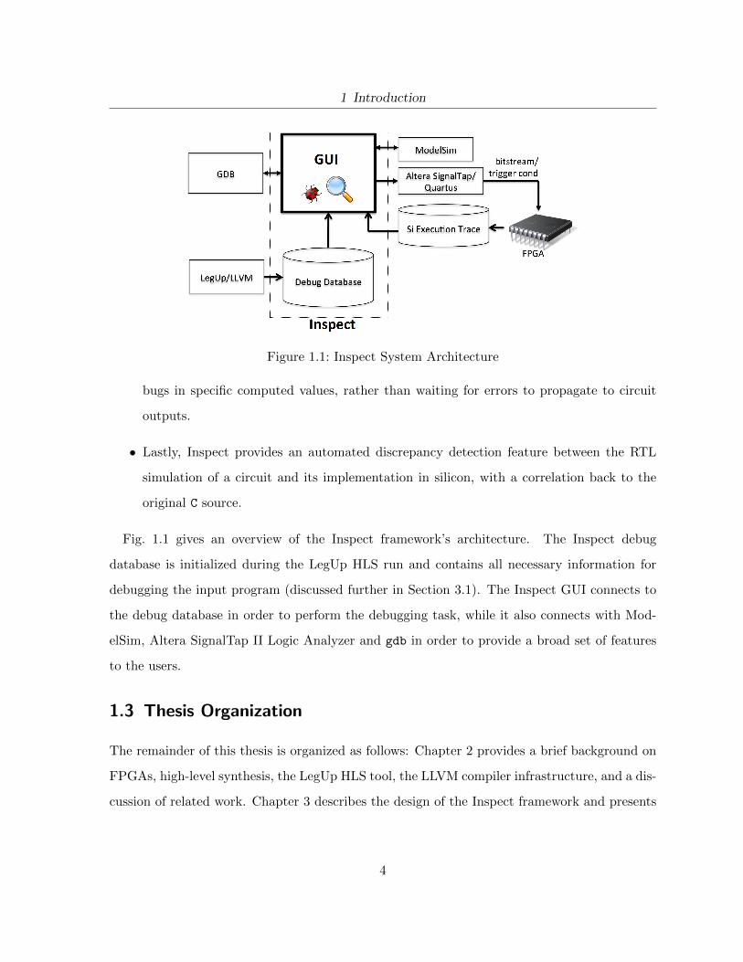
Figure 1.1: Inspect System Architecture
bugs in specific computed values, rather than waiting for errors to propagate to circuit
outputs.
• Lastly, Inspect provides an automated discrepancy detection feature between the RTL
simulation of a circuit and its implementation in silicon, with a correlation back to the
original C source.
Fig. 1.1 gives an overview of the Inspect framework’s architecture. The Inspect debug
database is initialized during the LegUp HLS run and contains all necessary information for
debugging the input program (discussed further in Section 3.1). The Inspect GUI connects to
the debug database in order to perform the debugging task, while it also connects with Mod-
elSim, Altera SignalTap II Logic Analyzer and gdb in order to provide a broad set of features
to the users.
1.3 Thesis Organization
The remainder of this thesis is organized as follows: Chapter 2 provides a brief background on
FPGAs, high-level synthesis, the LegUp HLS tool, the LLVM compiler infrastructure, and a dis-
cussion of related work. Chapter 3 describes the design of the Inspect framework and presents
4

1 Introduction
Inspect’s “debug database” and the framework’s features, as well as its integration with other
systems. Several case studies for different debugging scenarios are presented in Chapter 4 to
demonstrate how the Inspect debugger works. Chapter 5 discusses the framework’s imple-
mentation and provides information about the framework’s architecture. Chapter 6 presents
experimental results and demonstrates the effectiveness of the debugging framework to detect
bugs that are manually injected into the RTL produced by LegUp HLS. Finally, conclusions
and suggestions for future work are offered in Chapter 7.
5

2 Background and Related Work
2.1 Introduction
This chapter presents the background material forming the basis for the research. Section 2.2
gives an overview of field-programmable gate arrays (FPGAs). Section 2.3 reviews high-level
synthesis (HLS). Section 2.4 describes the LegUp HLS tool. Section 2.5 provides relevant
background on the LLVM framework and Section 2.6 surveys recent work on HLS debugging.
The chapter concludes with a summary in Section 2.7.
2.2 Field-Programmable Gate Arrays
An FPGA is an integrated circuit which can be programmed by the end user to implement
any digital circuit. Today, the most commonly used CAD flow for FPGAs requires the user to
specify the functionality of the desired circuit using a hardware description language (HDL),
such as VHDL or Verilog. FPGA vendors provide the tools to compile, synthesize, and place and
route the HDL design on an FPGA chip. FPGAs have several advantages over custom chips: 1)
they can be programmed in seconds, rather than requiring months of time for manufacturing;
2) they are cheaper than custom chips for all but the highest-volume applications; and 3) they
are re-configurable, which reduces the testing burden and allows designs to be verified on-chip.
The costs of IC manufacturing grow drastically with each technology node, and now stands
at tens of millions of dollars [28]. With custom chips, that cost must be borne by a single
application, whereas in FPGAs, that cost is amortized across all users of the device.
Modern FPGAs comprise an array of programmable logic blocks, I/Os, embedded SRAMs
and hard IP blocks, all of which may be connected to one another by way of a programmable in-
6

2 Background and Related Work
Figure 2.1: A simple schematic of an FPGA architecture.
terconnection (routing) network. The logic blocks consist mainly of look-up-tables and flip-flops,
with local routing. The hard IP blocks are more varied, and include DSP-oriented multiply/ac-
cumulate blocks, PCIe cores, and even entire processors. The purpose of the hard IP blocks
is to deliver higher speed and lower power for specific functions that FPGA vendors deem to
occur commonly in user designs.
Researchers around the world have been actively working on FPGA CAD algorithms, ar-
chitectures and circuits to reduce the gap between FPGAs and custom ASICs in terms of
area-efficiency, execution speed and power (e.g. [34, 37, 9]). Today, FPGAs are widely used for
many designs having requirements that used to be only met by ASICs. An abstract view of an
FPGA architecture is shown in Figure 2.1.
2.3 High-Level Synthesis
HLS raises the level of abstraction for hardware design by allowing software methodologies to
be used. HLS tools typically execute several tasks during the compilation of an input program
7
2 Background and Related Work
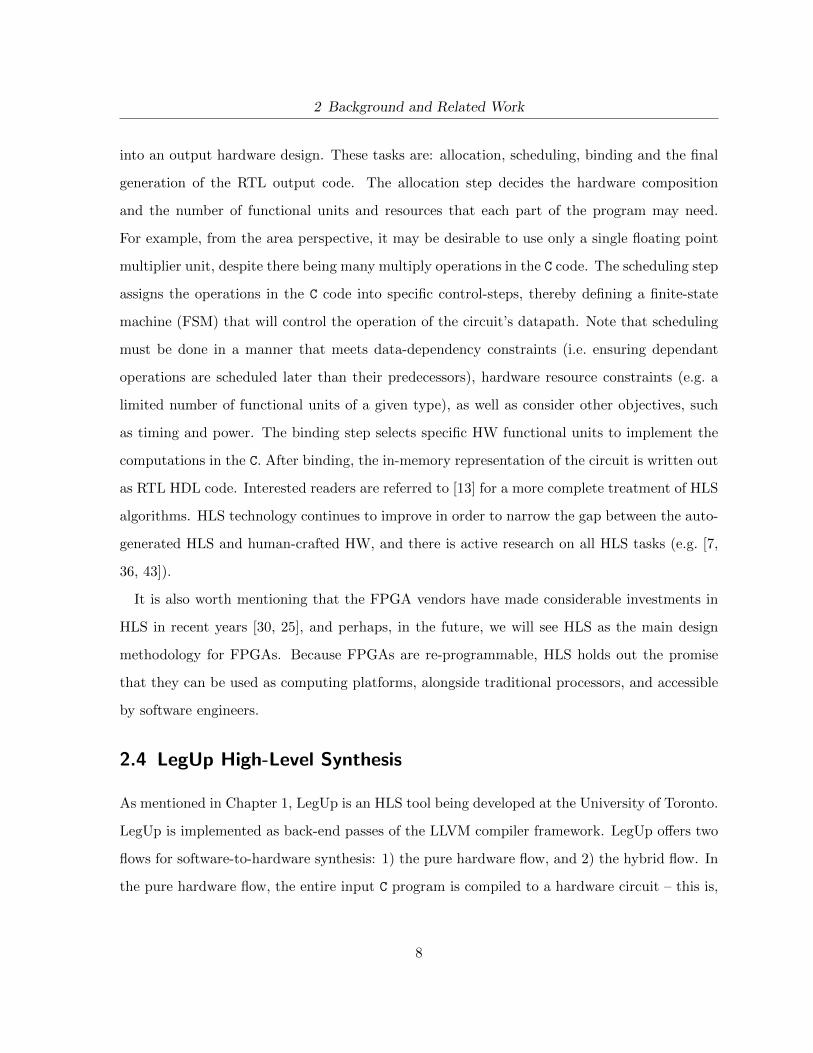
into an output hardware design. These tasks are: allocation, scheduling, binding and the final
generation of the RTL output code. The allocation step decides the hardware composition
and the number of functional units and resources that each part of the program may need.
For example, from the area perspective, it may be desirable to use only a single floating point
multiplier unit, despite there being many multiply operations in the C code. The scheduling step
assigns the operations in the C code into specific control-steps, thereby defining a finite-state
machine (FSM) that will control the operation of the circuit’s datapath. Note that scheduling
must be done in a manner that meets data-dependency constraints (i.e. ensuring dependant
operations are scheduled later than their predecessors), hardware resource constraints (e.g. a
limited number of functional units of a given type), as well as consider other objectives, such
as timing and power. The binding step selects specific HW functional units to implement the
computations in the C. After binding, the in-memory representation of the circuit is written out
as RTL HDL code. Interested readers are referred to [13] for a more complete treatment of HLS
algorithms. HLS technology continues to improve in order to narrow the gap between the auto-
generated HLS and human-crafted HW, and there is active research on all HLS tasks (e.g. [7,
36, 43]).
It is also worth mentioning that the FPGA vendors have made considerable investments in
HLS in recent years [30, 25], and perhaps, in the future, we will see HLS as the main design
methodology for FPGAs. Because FPGAs are re-programmable, HLS holds out the promise
that they can be used as computing platforms, alongside traditional processors, and accessible
by software engineers.
2.4 LegUp High-Level Synthesis
As mentioned in Chapter 1, LegUp is an HLS tool being developed at the University of Toronto.
LegUp is implemented as back-end passes of the LLVM compiler framework. LegUp offers two
flows for software-to-hardware synthesis: 1) the pure hardware flow, and 2) the hybrid flow. In
the pure hardware flow, the entire input C program is compiled to a hardware circuit – this is,
8
2 Background and Related Work
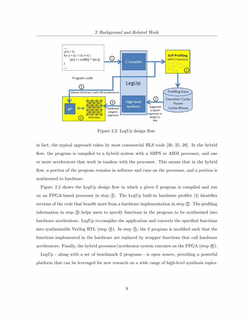
Figure 2.2: LegUp design flow.
in fact, the typical approach taken by most commercial HLS tools [30, 25, 20]. In the hybrid
flow, the program is compiled to a hybrid system with a MIPS or ARM processor, and one
or more accelerators that work in tandem with the processor. This means that in the hybrid
flow, a portion of the program remains in software and runs on the processor, and a portion is
synthesized to hardware.
Figure 2.2 shows the LegUp design flow in which a given C program is compiled and run
on an FPGA-based processor in step 1©. The LegUp built-in hardware profiler [4] identifies
sections of the code that benefit more from a hardware implementation in step 2©. The profiling
information in step 3© helps users to specify functions in the program to be synthesized into
hardware accelerators. LegUp re-compiles the application and converts the specified functions
into synthesizable Verilog RTL (step 4©). In step 5©, the C program is modified such that the
functions implemented in the hardware are replaced by wrapper functions that call hardware
accelerators. Finally, the hybrid processor/accelerator system executes on the FPGA (step 6©).
LegUp - along with a set of benchmark C programs - is open source, providing a powerful
platform that can be leveraged for new research on a wide range of high-level synthesis topics.
9

2 Background and Related Work
For more details, the reader is referred to [8].
While the LegUp system provides both the pure hardware flow and the hybrid flow, in this
thesis, we centre on debugging methodologies for the pure hardware flow. Debugging approaches
for the hybrid flow, with a processor concurrently operating with accelerators, is left to future
work.
2.5 LLVM
LLVM is an open-source compiler framework widely used in industry and academia [27].
LLVM’s front-end, clang, parses and converts a C or C++ program into LLVM’s intermedi-
ate representation (IR)1. The IR closely resembles assembly code, wherein the computations
and control flow of the program are represented as simple instructions (e.g. shift, multiply, add,
branch, and so on). Following conversion to the IR, the program is optimized using a wide
variety of optimization passes. Finally, LLVM’s back-end is invoked to generate machine code
for a target processor.
When LLVM converts an input program into its IR and then optimizes the IR, it generates
what is called debug metadata. Debug metadata is “side information” that allows one to link
the instructions in the IR with the original lines of C source code. It contains, for example,
for each IR instruction, the line number in the original source code, the function, and so on.
Such information is also (partially) retained after passes of IR optimization. In this work, we
leverage the LLVM metadata to link the C with the IR, and then with the Verilog produced by
LegUp.
Figure 2.3 shows a sample C code, the corresponding generated LLVM IR code and the
associated LLVM debug metadata. The C program defines three local variables (x, y, and z).
The decimal values of 5 and 10 are stored in variables x and y respectively and the value of the
x + y statement is kept in the variable z and is returned as the output. The LLVM IR code
resembles the C program in the IR level and the LLVM debug metadata defines the mapping
1LLVM also provides front ends for other languages, such as Java.
10

2 Background and Related Work
Figure 2.3: LLVM debug metadata.
between LLVM program objects and source-level objects. The “subprogram descriptor” in the
debug metadata contains information such as line number, column number, name, file location.
for the func A function in the C code. LLVM instructions are attached with location information
descriptors specifying their corresponding line and column number in the C code. For example,
the add instruction in LLVM IR code is related to line 4 in the C code. For further information
about LLVM debug data and a full list of the LLVM debug descriptors, interested readers are
referred to [27].
2.6 Related Work
Debugging for HLS is a relatively new area of research, as HLS has recently received widespread
attention and use. Moreover, the first users of HLS have been engineers with HW design skills,
making hardware debugging methods possible to use for them, but difficult to be applied on
auto-generated HLS designs. As adoption of HLS spreads to those without hardware skills,
11
2 Background and Related Work
having HLS-specific debugging strategies is increasingly necessary.
This section will discuss the previous work in the field of hardware and HLS debugging.
2.6.1 High-Level Synthesis Debugging
Academic Research
The work of Hemmert et al. on the Sea Cucumber HLS Debugger (SC Debugger) most closely
resembles our own [18, 39]. It provides source-level debugging capabilities for hardware designs
in the context of an original Java source. The Sea Cucumber (SC) is an HLS tool that uses a
VLIW-like2 compilation flow to generate an optimized hardware design for the input program.
It accepts Java class files - which are the results of compiling the Java source codes - as in-
puts and generates JHDL circuits as outputs. JHDL is a structural HDL implemented with
Java [32]. The SC Debugger works on top of the SC HLS tool and provides a feature set similar
to a typical software debugger including: single-stepping, setting/watching variables values,
and breakpoints. Like Inspect, it also offers two debugging approaches (“hardware-centric”
and “software-centric”) to give an illusion of different HW/SW execution. The SC Debugger
supports debugging in the presence of optimizations such as predictions and block merging, and
similar to Inspect offers two modes for debugging: simulation and silicon debugging.
Key differences between Inspect and SC Debugger are as follows:
1) The Inspect framework is built as part of the LegUp HLS tool which enables debugging for
designs originally written in C, while the SC Debugger is built on top of the Sea Cucumber
HLS tool, which translates Java source code to JHDL.
2) Function calls are not supported in the SC Debugger, while Inspect handles function calls
and provides two different modes, including step-over and step-in, for such calls.
3) Inspect has an automated HW/SW discrepancy detection feature that allows users to find
bugs in the design as soon as they occur.
2Very Long Instruction Word
12
2 Background and Related Work
...
start = clock();
...
//lines of code to be verified
...
end = clock();
time = end - start;
assert (time > 10 );
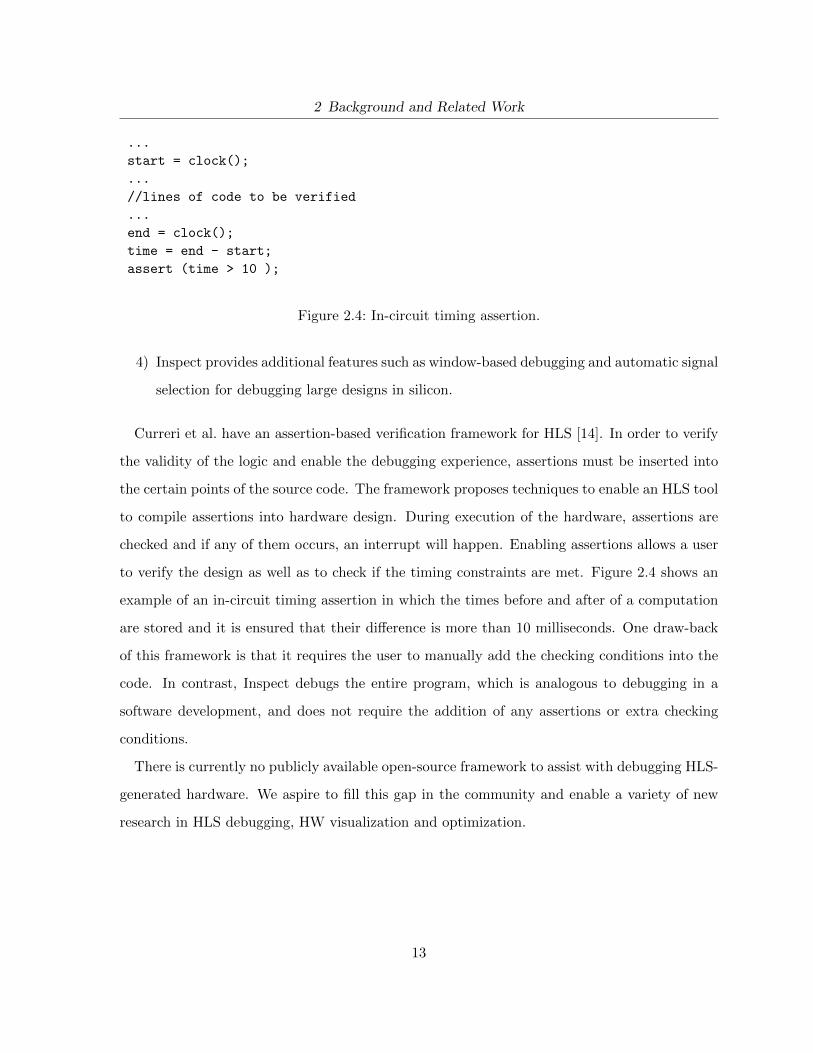
Figure 2.4: In-circuit timing assertion.
4) Inspect provides additional features such as window-based debugging and automatic signal
selection for debugging large designs in silicon.
Curreri et al. have an assertion-based verification framework for HLS [14]. In order to verify
the validity of the logic and enable the debugging experience, assertions must be inserted into
the certain points of the source code. The framework proposes techniques to enable an HLS tool
to compile assertions into hardware design. During execution of the hardware, assertions are
checked and if any of them occurs, an interrupt will happen. Enabling assertions allows a user
to verify the design as well as to check if the timing constraints are met. Figure 2.4 shows an
example of an in-circuit timing assertion in which the times before and after of a computation
are stored and it is ensured that their difference is more than 10 milliseconds. One draw-back
of this framework is that it requires the user to manually add the checking conditions into the
code. In contrast, Inspect debugs the entire program, which is analogous to debugging in a
software development, and does not require the addition of any assertions or extra checking
conditions.
There is currently no publicly available open-source framework to assist with debugging HLS-
generated hardware. We aspire to fill this gap in the community and enable a variety of new
research in HLS debugging, HW visualization and optimization.
13
2 Background and Related Work
Commercial Tools
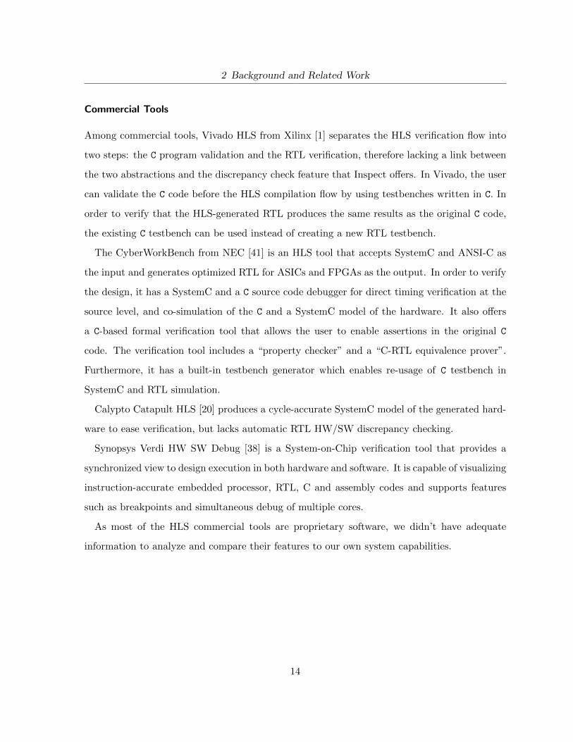
Among commercial tools, Vivado HLS from Xilinx [1] separates the HLS verification flow into
two steps: the C program validation and the RTL verification, therefore lacking a link between
the two abstractions and the discrepancy check feature that Inspect offers. In Vivado, the user
can validate the C code before the HLS compilation flow by using testbenches written in C. In
order to verify that the HLS-generated RTL produces the same results as the original C code,
the existing C testbench can be used instead of creating a new RTL testbench.
The CyberWorkBench from NEC [41] is an HLS tool that accepts SystemC and ANSI-C as
the input and generates optimized RTL for ASICs and FPGAs as the output. In order to verify
the design, it has a SystemC and a C source code debugger for direct timing verification at the
source level, and co-simulation of the C and a SystemC model of the hardware. It also offers
a C-based formal verification tool that allows the user to enable assertions in the original C
code. The verification tool includes a “property checker” and a “C-RTL equivalence prover”.
Furthermore, it has a built-in testbench generator which enables re-usage of C testbench in
SystemC and RTL simulation.
Calypto Catapult HLS [20] produces a cycle-accurate SystemC model of the generated hard-
ware to ease verification, but lacks automatic RTL HW/SW discrepancy checking.
Synopsys Verdi HW SW Debug [38] is a System-on-Chip verification tool that provides a
synchronized view to design execution in both hardware and software. It is capable of visualizing
instruction-accurate embedded processor, RTL, C and assembly codes and supports features
such as breakpoints and simultaneous debug of multiple cores.
As most of the HLS commercial tools are proprietary software, we didn’t have adequate
information to analyze and compare their features to our own system capabilities.
14

2 Background and Related Work
2.6.2 On-Chip Debugging for FPGAs
Academic Research
There are several works on circuit debugging using trace buffers, which are on-chip memories
that “record” the values of selected signals during circuit run, usually for a specific window
of time or when specific events happen within the circuit. “Triggers” are sub-circuits that are
added to the circuit that control when signal values should be stored in trace buffers. The
work of Hung et al. [31] on speculative debug insertion for FPGAs, automatically inserts trace
buffers and “observation circuits” for signals before compilation and tries to detect the most
valuable signals to be probed. Determining the most important signals to be probed is very
crucial for debugging large designs, as memory and I/O limitations make it impossible to track
all signals.
The work of Graham on Logical Hardware Debugger for FPGA-Based Systems [16] is among
the first works that enables software-like debugging capabilities for designs generated at a low
level of abstraction. It offers a logical hardware debugger for FPGA systems which provides an
insight into debugging circuits at the structural level by creating a logical to physical mapping.
This work is done in JHDL CAD tool - a Java based design environment - [32] and used as a
basis for the Sea Cucumber debugger.
Commercial Tools
For debugging in silicon, Xilinx ChipScope Pro [3] and Altera SignalTap II [6] automatically
insert trace buffers and trigger circuitry to allow a pre-selected set of signals to be visible in
the silicon run. Though these tools offer useful silicon debugging capabilities, they need to
be manually configured by the user. Moreover, debugging information is displayed in their
framework’s environment and does not provide a strong insight into the original HDL source
code. Certus from Mentor Graphics [2] also offers similar silicon debug functionality, with the
ability to observe a greater number of signals.
15

2 Background and Related Work
2.7 Summary
This chapter introduced the topics relevant to the proposed debugging research: FPGAs, high-
level synthesis, the LegUp framework and its underlying LLVM compiler infrastructure. We
also discussed related work on debugging for HLS, both in the academia and industrial contexts,
as well as an overview of on-chip debugging approaches.
16

3 Source-Level Debugging Framework Design
Software debuggers usually work with two abstraction levels: source-level and assembly-level.
Software debuggers execute the low-level assembly and through debug metadata link the low-
level execution with the high-level source code. The execution of the assembly is controlled
by the user via the source code, allowing the user to step, continue, set breakpoints, and so
on. The user can also view the values of variables as execution proceeds, set watchpoints,
and see the program’s call stack. In essence, from the user’s perspective, the execution and
debugging appears to be happening at the source level, while underneath, it is in fact happening
at a lower level. Our debugging approach for HLS mirrors this behaviour – the user interacts
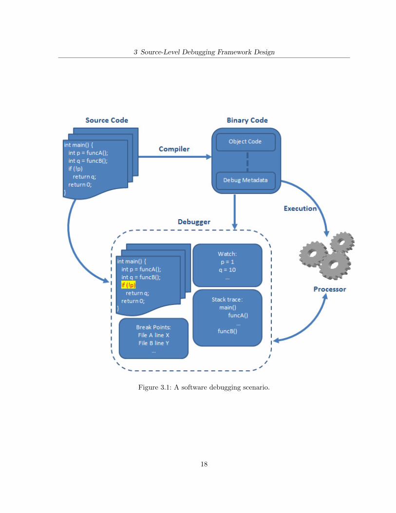
at the source level, while execution is actually happening at the hardware level. Figure 3.1
illustrates a software debugger’s interactions with other tools in a software-debug scenario. A
program written in a high-level language is compiled to binary code by a compiler. The binary
code is executed on a processor. The debugger reads the program’s debug metadata from the
binary code and controls the execution of the program on the processor, while showing relevant
source-level information to the user.
Designing a debugger for HLS differs considerably from designing a software debugger, with
a key difference being there are now three levels of abstraction that must be linked together
instead of two. In HLS, the source code is first compiled and optimized at the compiler’s
IR level (similar to assembly). Subsequently, the IR is input to HLS to produce the HW.
HLS debuggers must therefore map between the source code and the IR on one side, and also
between the IR and HW on the other side. The former is straightforward, as the mapping is
similar to typical software debugger design. However, the latter is more complicated, not only
17
3 Source-Level Debugging Framework Design
Figure 3.1: A software debugging scenario.
18
3 Source-Level Debugging Framework Design
because the mapping is specific to HLS and has not been addressed before, but also because
there are inherent differences between the two sides of the mapping. The IR code is low-
level software code that still has the sequential structure of the original source code and runs
sequentially on a processor. On the other hand, the hardware design is inherently parallel with
a completely different structure. The HW parallelism results in more than one IR instruction
being executed at one time. The HW may also have functional units that are shared between
different IR operations, as long as those operations are scheduled in different HW clock cycles.
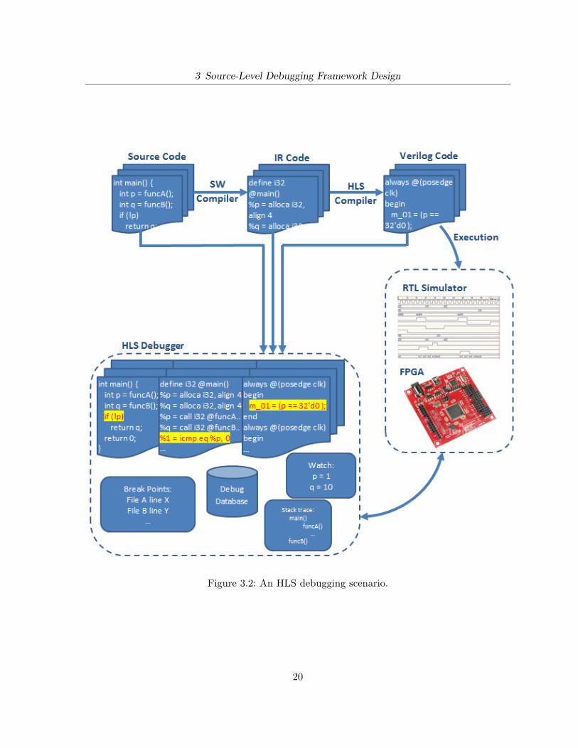
Such differences are critical to the design of an HLS debugger. Figure 3.2 shows the HLS debug
scenario and demonstrates an HLS debugger’s interactions with the environment. A program
written in a high-level language goes through a software compiler and an HLS flow, generating
low-level software code (IR) and a hardware design. The hardware design either runs on an
FPGA or an RTL simulator. An HLS debugger is tightly coupled with the HLS tool and uses the
HLS data in order to create a debug database (containing all necessary relationships between
different compilation stages) and provide visibility at all abstraction levels (C, IR, Hardware).
In this chapter, we first introduce Inspect’s debug database, which we generate to link between
the three abstraction levels. The three abstraction levels in HLS are discussed in detail in
Sections 3.2, 3.3 and 3.4. Inspect’s “debug engine” that provides the core functionality for
the simulation and silicon debug modes is presented in Section 3.5. Lastly, the features of the
Inspect framework are discussed in Section 3.6.
3.1 Debug Database
Inspect extracts the debug metadata from the LLVM IR instructions and keeps all data and
relationships between the source-level, IR-level and hardware-level abstractions in the debug
database. For example, using the debug database, LLVM IR instructions for each line of C code,
as well as the corresponding Verilog code and HW signal names for each LLVM IR instruction
can be found. A simplified view of the debug database is shown in Figure 3.31. Each box
1Figure is auto-generated by the MySQL Workbench tool.
19
3 Source-Level Debugging Framework Design
Figure 3.2: An HLS debugging scenario.
20

3 Source-Level Debugging Framework Design
Figure 3.3: Simplified schema of Inspect’s debug database.
represents a data record (some internal fields are not shown for clarity), and edges represent
relationships between corresponding records. Note that edge ends have labels that convey 0-
to-many relationships. For example, the edge between “HW signal” and “variable” boxes, has
a “1” on one end of the edge and “0..1” on the other end of the edge. These labels indicate
that every hardware signal is associated with 0 or 1 variables in the C code - There are many
signals in the HW that have no corresponding C variable, hence the possibility of 0. Also,
solid lines represent identifying relationship between the entities meaning that the existence of
a row in the child table depends on a row in the parent table, while the dotted lines represent
non-identifying relationships which express the relation between the entities that do not depend
on each other. For instance, the records in the IRState table are only meaningful when they
are linked to a parent record in both IRInstr and State tables, hence defining an identifying
relationship.
The key pieces of information in the debug database are:
1. High-Level C statements: Inspect tracks each statement’s line and column number in
the C file. With this information, Inspect can operate with statements rather than lines.
21

3 Source-Level Debugging Framework Design
This is useful in situations when either one source line contains more than one statement,
such as in for loops, or if the input source file is not well formatted.
2. IR instructions: contains all information about the LLVM IR instructions, including
the function containing each instruction, the instruction’s text and its position (order)
in the function. The relationships among the IR instructions, functions and high-level
statements are also preserved in the debug database. However, there are some IR in-
structions that do not have any link to a high-level statement, due to either compiler
optimizations or a lack of debug metadata. A high-level statement can link to more than
one IR instruction creating a one-to-many relationship.
3. States: state records are the most important piece of information that Inspect uses to
control the execution of the program. State records contain information about LegUp’s
FSM, including the IR instructions scheduled in each state and the sets of signals whose
values may be affected. LegUp’s FSM is discussed further in Section 3.3. In LegUp, IR
instructions may take one or more cycles to execute (i.e. there may exist multi-cycle op-
erations), therefore, each IR instruction has links to an IRState record defining its start
and end states (startStateId and endStateId fields). LegUp states that handle store in-
structions have more information to preserve: 1) the HW signal that corresponds to the
variable being updated and its byte offset, and 2) the memory port in which the value is
being read/written from/to. Currently there can be up to two store instructions sched-
uled in each state in LegUp designs. This information is preserved in “StateStoreInfo”
records.
4. Functions: LegUp generates a Verilog module for each function in the C program. Inspect
tracks the names and file line numbers of all C functions compiled to hardware. Most of the
Inspect database entities including variables, IR instructions and HW signals are linked
to a function record, implying the function they belong to. High-level statements are also
linked to functions through their relationship to IR instructions. Each state has links to a
22
3 Source-Level Debugging Framework Design
function record, specifying the function in which the state is defined (belongingFunctionId)
and the function that the state may call, if it is a call state (calledFunctionId). By tracking
the function calls, Inspect is capable of providing call stack information to users.
5. HW signals: stores information about the hardware design signals. This includes the
signal name, bit-width, the C function it belongs to (equivalent to the signal’s Verilog
module), and so on. LegUp generates one or more signals for each IR instruction, reflected
in “InstructionSignal” records.
6. Variables: contains all necessary information about RAM modules instantiated by
LegUp, as well as LLVM IR variables. Address width, data width, tag number2, size
(number of elements), and variable data types, are stored for each variable record. Com-
plex variable types such as array, struct and combinations of them are also supported
by Inspect. Variables have three types of relationships with other entities: 1) a link to a
function record representing the function in which the variable is declared, 2) a link to a
HW signal record representing the signal that provides the value for the variable, and 3)
a link to an IR instruction record representing the allocation instruction (LLVM alloca)
for the variable. More information on the variables can be found in Section 3.3.
Inspect’s debug database is built within the MySQL database management system [29].
3.2 Hardware-Level View
As discussed in Section 2.4, LegUp HLS works with three different abstraction levels of the
program. The lowest level of abstraction is the hardware design, as specified in the Verilog file
automatically generated by LegUp. The design file is usually very large with tens of thousands
of lines and thus, it is not easy to understand or debug.
2LegUp handles memory by instantiating RAMs in the HDL for arrays, structures and other data, and instan-tiating a memory controller to steer data to/from the correct RAM instance. 32-bit memory addresses arepartitioned by LegUp into a 9-bit tag, and a 23-bit address. The memory controller uses the 9-bit tag touniquely specify the RAM instance to access. The assigning of tags to data is done automatically duringHLS.
23

3 Source-Level Debugging Framework Design
Figure 3.4: Verilog code blocks for a load instruction.
24

3 Source-Level Debugging Framework Design
Figure 3.5: Inspect’s hardware watch table.
Inspect’s GUI dedicates a panel to the hardware-level view of the program. There is frequently
more than one code block in the Verilog related to a specific IR instruction. For example,
Figure 3.4 shows five “always blocks” in different locations of the Verilog file that are related
to one LLVM load instruction.
During the debugging session, the user can click on any IR instruction and see the related
Verilog code blocks in the hardware-view panel.
Besides the ability to show Verilog code blocks, Inspect also provides a watch table for
hardware signals. The “hardware watch table” shows the updated values for all hardware
signals related to the current state of execution. Signals in the hardware watch table are usually
related to concepts from higher abstraction levels (e.g. IR instructions and C statements). The
hardware watch table displays the values in hexadecimal format. Figure 3.5 displays Inspect’s
hardware watch table for all hardware signals and their values grouped by their corresponding
IR instructions in one specific cycle.
3.3 IR-Level View
LegUp HLS accepts optimized LLVM IR code as its input. While IR instructions execute in
a sequential manner, the hardware design that they are compiled into is inherently parallel.
25
3 Source-Level Debugging Framework Design
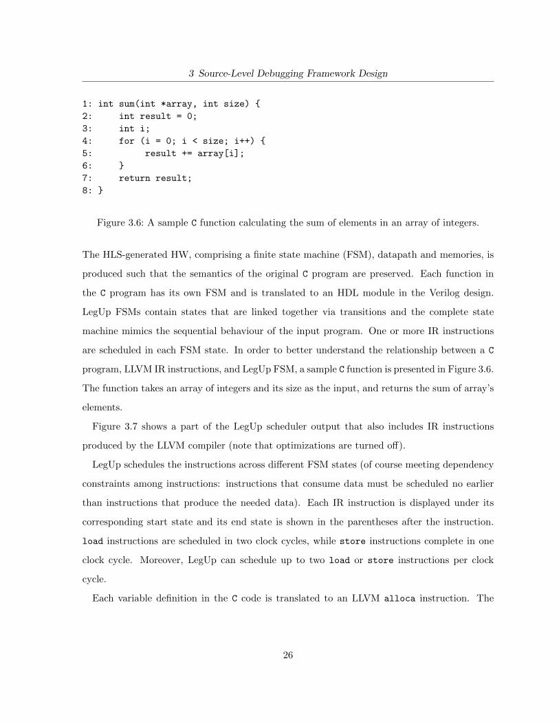
1: int sum(int *array, int size) {
2: int result = 0;
3: int i;
4: for (i = 0; i < size; i++) {
5: result += array[i];
6: }
7: return result;
8: }
Figure 3.6: A sample C function calculating the sum of elements in an array of integers.
The HLS-generated HW, comprising a finite state machine (FSM), datapath and memories, is
produced such that the semantics of the original C program are preserved. Each function in
the C program has its own FSM and is translated to an HDL module in the Verilog design.
LegUp FSMs contain states that are linked together via transitions and the complete state
machine mimics the sequential behaviour of the input program. One or more IR instructions
are scheduled in each FSM state. In order to better understand the relationship between a C
program, LLVM IR instructions, and LegUp FSM, a sample C function is presented in Figure 3.6.
The function takes an array of integers and its size as the input, and returns the sum of array’s
elements.
Figure 3.7 shows a part of the LegUp scheduler output that also includes IR instructions
produced by the LLVM compiler (note that optimizations are turned off).
LegUp schedules the instructions across different FSM states (of course meeting dependency
constraints among instructions: instructions that consume data must be scheduled no earlier
than instructions that produce the needed data). Each IR instruction is displayed under its
corresponding start state and its end state is shown in the parentheses after the instruction.
load instructions are scheduled in two clock cycles, while store instructions complete in one
clock cycle. Moreover, LegUp can schedule up to two load or store instructions per clock
cycle.
Each variable definition in the C code is translated to an LLVM alloca instruction. The
26

3 Source-Level Debugging Framework Design
1 : state: LEGUP_0
2 : Transition: if (start): LEGUP_F_sum_BB_0_1 default: LEGUP_0
3 : state: LEGUP_F_sum_BB_0_1
4 : %1 = alloca i32*, align 4 (endState: LEGUP_F_sum_BB_0_1)
5 : %2 = alloca i32, align 4 (endState: LEGUP_F_sum_BB_0_1)
6 : %result = alloca i32, align 4 (endState: LEGUP_F_sum_BB_0_1)
7 : %i = alloca i32, align 4 (endState: LEGUP_F_sum_BB_0_1)
8 : store i32* %array, i32** %1, align 4 (endState: LEGUP_F_sum_BB_0_2)
9 : store i32 %size, i32* %2, align 4 (endState: LEGUP_F_sum_BB_0_2)
10: Transition: default: LEGUP_F_sum_BB_0_2
11: state: LEGUP_F_sum_BB_0_2
12: store i32 0, i32* %result, align 4, !dbg !20 (endState: LEGUP_F_sum_BB_0_3)
13: store i32 0, i32* %i, align 4, !dbg !23 (endState: LEGUP_F_sum_BB_0_3)
14: Transition: default: LEGUP_F_sum_BB_0_3
15: state: LEGUP_F_sum_BB_0_3
16: br label %3, !dbg !23
17: Transition: default: LEGUP_F_sum_BB_3_4
18: state: LEGUP_F_sum_BB_3_4
19: %4 = load i32* %i, align 4, !dbg !23 (endState: LEGUP_F_sum_BB_3_6)
20: %5 = load i32* %2, align 4, !dbg !23 (endState: LEGUP_F_sum_BB_3_6)
21: Transition: default: LEGUP_F_sum_BB_3_5
22: state: LEGUP_F_sum_BB_3_5
23: Transition: default: LEGUP_F_sum_BB_3_6
24: state: LEGUP_F_sum_BB_3_6
25: %6 = icmp slt i32 %4, %5, !dbg !23 (endState: LEGUP_F_sum_BB_3_6)
26: br i1 %6, label %7, label %17, !dbg !23
27: Transition: if (%6): LEGUP_F_sum_BB_7_7 default: LEGUP_F_sum_BB_17_17
28: state: LEGUP_F_sum_BB_7_7
29: %8 = load i32* %i, align 4, !dbg !24 (endState: LEGUP_F_sum_BB_7_9)
30: %9 = load i32** %1, align 4, !dbg !24 (endState: LEGUP_F_sum_BB_7_9)
31: Transition: default: LEGUP_F_sum_BB_7_8
32: state: LEGUP_F_sum_BB_7_8
33: %12 = load i32* %result, align 4, !dbg !24 (endState: LEGUP_F_sum_BB_7_10)
34: Transition: default: LEGUP_F_sum_BB_7_9
35: state: LEGUP_F_sum_BB_7_9
36: %10 = getelementptr inbounds i32* %9, i32 %8, !dbg !24 (endState: LEGUP_F_sum_BB_7_9)
37: %11 = load i32* %10, !dbg !24 (endState: LEGUP_F_sum_BB_7_11)
38: Transition: default: LEGUP_F_sum_BB_7_10
39: state: LEGUP_F_sum_BB_7_10
40: Transition: default: LEGUP_F_sum_BB_7_11
41: state: LEGUP_F_sum_BB_7_11
42: %13 = add nsw i32 %12, %11, !dbg !24 (endState: LEGUP_F_sum_BB_7_11)
43: store i32 %13, i32* %result, align 4, !dbg !24 (endState: LEGUP_F_sum_BB_7_12)
44: Transition: default: LEGUP_F_sum_BB_7_12
45: ...
46: ...
Figure 3.7: A part of the LLVM IR and LegUp scheduler output for the given example inFigure 3.6.
27

3 Source-Level Debugging Framework Design
alloca instruction allocates specified bytes of memory on the runtime stack frame to the
variable. For the given example, there are four variables defined in the C code: array and size
that are input arguments to the function and result and i which are local variables. Lines 4 -
7 of the scheduler output show the allocation instructions for these variables. Inspect recognizes
C variables and their name by tracking these alloca instructions.
The load instruction is used when a variable value is required. For example in line 4 of the
C code, variables i and size are needed to perform the i < size comparison. Lines 19 and 20
in the scheduler output show the corresponding required load instructions.
The getelementptr instruction is used to compute the address of the accessing index in
composite type (array and struct) variables. For example, lines 29 - 43 of the scheduler
output show the instructions to perform the result += array[i] statement in line 5 of the
C code: first a load instruction in line 30 is used to get the starting address of the array
variable. Then a getelementptr instruction in line 36 is used to calculate the address for the
i’th index of the variable. The getelementptr instruction accepts the index value (%8) and
the base address (%9) and returns the address for the i’th index (%10). Finally, another load
instruction is used to obtain the actual value of the i’th index by having the calculated address
(line 37).
The store instruction is used when there is an assignment updating the variable. For ex-
ample, line 5 of the C code stores the value of result + array[i] statement into the result
variable. This translates to the store instruction in line 43 of the scheduler output.
For more detailed information about LLVM instructions, interested readers are referred to
Appendix B.
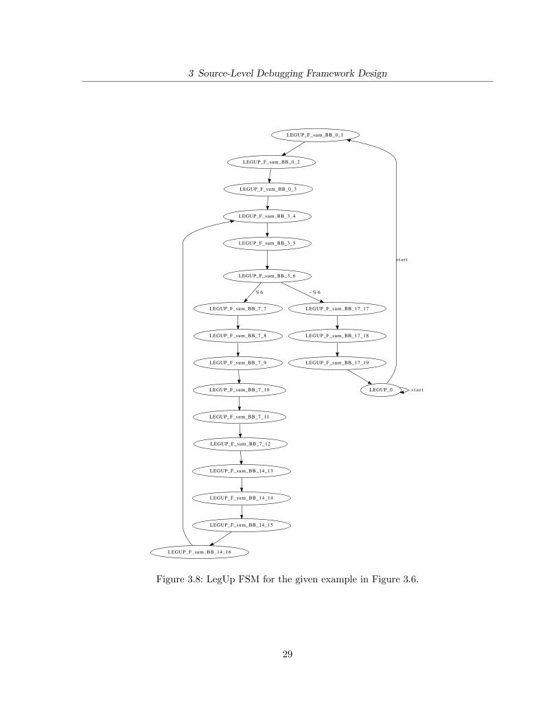
Figure 3.8 shows the FSM for the given example. LegUp starts from the initial state of
the FSM and traverses the state machine, executing corresponding IR instructions in each
state. Branch instructions create conditional transitions in the FSM. For example in the Fig-
ure 3.8, the state labelled LEGUP F sum BB 3 6 is a conditional state that proceeds to either
LEGUP F sum BB 7 7 or LEGUP F sum BB 17 17 depending on the value of variable %6. This
28
3 Source-Level Debugging Framework Design
LEGUP_F_sum_BB_0_1
LEGUP_F_sum_BB_0_2
LEGUP_0
s t a r t
~ s t a r t
LEGUP_F_sum_BB_0_3
LEGUP_F_sum_BB_3_4
LEGUP_F_sum_BB_3_5
LEGUP_F_sum_BB_3_6
LEGUP_F_sum_BB_7_7
%6
LEGUP_F_sum_BB_17_17
~ % 6
LEGUP_F_sum_BB_7_8 LEGUP_F_sum_BB_17_18
LEGUP_F_sum_BB_7_9
LEGUP_F_sum_BB_7_10
LEGUP_F_sum_BB_7_11
LEGUP_F_sum_BB_7_12
LEGUP_F_sum_BB_14_13
LEGUP_F_sum_BB_14_14
LEGUP_F_sum_BB_14_15
LEGUP_F_sum_BB_14_16
LEGUP_F_sum_BB_17_19
Figure 3.8: LegUp FSM for the given example in Figure 3.6.
29

3 Source-Level Debugging Framework Design
Figure 3.9: LegUp FSM function call example.
conditional state transition is related to the LLVM br (branch) instruction in line 26 of the
Figure 3.7 and C statement i < size in line 4 of the Figure 3.6. LegUp returns to the initial
state where the execution was started from, when all computations are completed.
Function calls translate into a special case of FSM conditional states in which the function
call state in the “calling” function branches to itself (does not proceed) until a signal indi-
cating the return from the “called” function becomes true. Figure 3.9 shows a portion of the
FSM for a main function that calls the sum function in Figure 3.6. The FSM stays in the
LEGUP function call 41 state until the sum finish final signal becomes true, indicating the
completion of the sum function. Inspect keeps track of all state transitions and builds a “call
stack” using the FSM call states. This enables Inspect to handle multi-function programs.
Inspect’s variable/signal watching feature uses the call stack information in order to display
the values of variables/signals that are in the program/circuit’s active scope. This feature is
discussed further in Section 3.6.3.
The IR-view panel of the debugger is shown in the right side of Figure 3.10. IR instructions
are grouped by their corresponding FSM state. Based on the FSM’s active state, there is a
list of executing IR instructions and corresponding C statements. Inspect highlights all parallel
executing C statements: the currently focused statement is highlighted yellow (line 10), while
the other executing statements are highlighted green (line 8). By issuing “step” commands,
Inspect navigates the user through the current active statements in order to better visualize the
program/circuit’s execution. Clicking on any active C statement highlights its corresponding
IR instructions across all states. Figure 3.10 shows the corresponding IR instructions for the C
30

3 Source-Level Debugging Framework Design
Figure 3.10: Source-view and IR-view panel of the Inspect debugger.
statement on line 10. Operations in line 10 span through 5 different FSM states because of the
dependencies and the limitations on parallel memory operations in LegUp. The current active
state in the figure is State #2 and its related IR instructions are highlighted in yellow. While
the rest of IR instructions that are set to execute in next clock cycles but are still related to
the current line number (line 10) are highlighted in faded yellow (States 3, 4, 5 and 6).
3.4 Source-Level View
The actual C program – the highest abstraction level – is shown in the source-level panel. Some C
source characteristics, such as the location of statements, functions, and variables, are detected
by Inspect. This information is used to infer the relationship between the IR instructions and
the C code as it is discussed in Section 3.3. The information is extracted from LLVM debug
metadata and could be corrupted or completely lost if compiler optimizations are enabled.
Figure 3.10 shows Inspect’s source-level panel in the left side.
31
3 Source-Level Debugging Framework Design
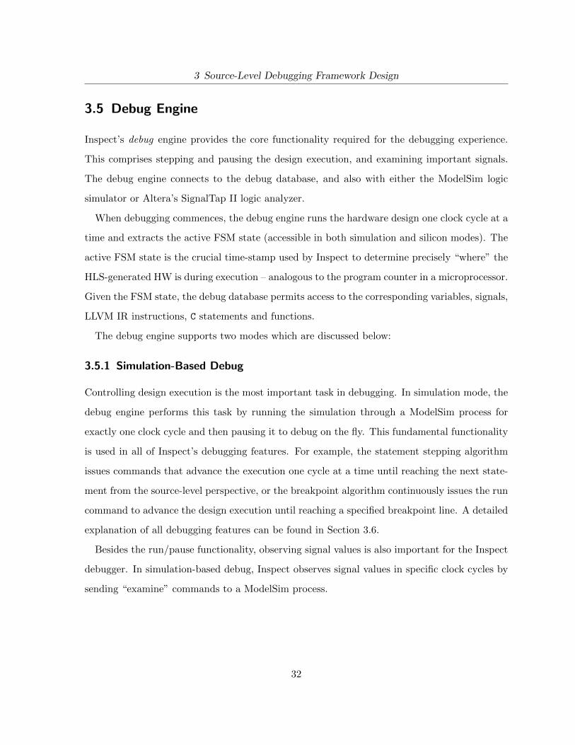
3.5 Debug Engine
Inspect’s debug engine provides the core functionality required for the debugging experience.
This comprises stepping and pausing the design execution, and examining important signals.
The debug engine connects to the debug database, and also with either the ModelSim logic
simulator or Altera’s SignalTap II logic analyzer.
When debugging commences, the debug engine runs the hardware design one clock cycle at a
time and extracts the active FSM state (accessible in both simulation and silicon modes). The
active FSM state is the crucial time-stamp used by Inspect to determine precisely “where” the
HLS-generated HW is during execution – analogous to the program counter in a microprocessor.
Given the FSM state, the debug database permits access to the corresponding variables, signals,
LLVM IR instructions, C statements and functions.
The debug engine supports two modes which are discussed below:
3.5.1 Simulation-Based Debug
Controlling design execution is the most important task in debugging. In simulation mode, the
debug engine performs this task by running the simulation through a ModelSim process for
exactly one clock cycle and then pausing it to debug on the fly. This fundamental functionality
is used in all of Inspect’s debugging features. For example, the statement stepping algorithm
issues commands that advance the execution one cycle at a time until reaching the next state-
ment from the source-level perspective, or the breakpoint algorithm continuously issues the run
command to advance the design execution until reaching a specified breakpoint line. A detailed
explanation of all debugging features can be found in Section 3.6.
Besides the run/pause functionality, observing signal values is also important for the Inspect
debugger. In simulation-based debug, Inspect observes signal values in specific clock cycles by
sending “examine” commands to a ModelSim process.
32
3 Source-Level Debugging Framework Design
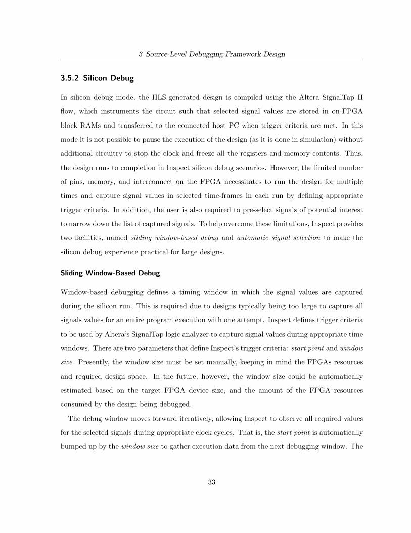
3.5.2 Silicon Debug
In silicon debug mode, the HLS-generated design is compiled using the Altera SignalTap II
flow, which instruments the circuit such that selected signal values are stored in on-FPGA
block RAMs and transferred to the connected host PC when trigger criteria are met. In this
mode it is not possible to pause the execution of the design (as it is done in simulation) without
additional circuitry to stop the clock and freeze all the registers and memory contents. Thus,
the design runs to completion in Inspect silicon debug scenarios. However, the limited number
of pins, memory, and interconnect on the FPGA necessitates to run the design for multiple
times and capture signal values in selected time-frames in each run by defining appropriate
trigger criteria. In addition, the user is also required to pre-select signals of potential interest
to narrow down the list of captured signals. To help overcome these limitations, Inspect provides
two facilities, named sliding window-based debug and automatic signal selection to make the
silicon debug experience practical for large designs.
Sliding Window-Based Debug
Window-based debugging defines a timing window in which the signal values are captured
during the silicon run. This is required due to designs typically being too large to capture all
signals values for an entire program execution with one attempt. Inspect defines trigger criteria
to be used by Altera’s SignalTap logic analyzer to capture signal values during appropriate time
windows. There are two parameters that define Inspect’s trigger criteria: start point and window
size. Presently, the window size must be set manually, keeping in mind the FPGAs resources
and required design space. In the future, however, the window size could be automatically
estimated based on the target FPGA device size, and the amount of the FPGA resources
consumed by the design being debugged.
The debug window moves forward iteratively, allowing Inspect to observe all required values
for the selected signals during appropriate clock cycles. That is, the start point is automatically
bumped up by the window size to gather execution data from the next debugging window. The
33

3 Source-Level Debugging Framework Design
Figure 3.11: Inspect window-based debug.
process of window-based debugging is automated and is performed by Inspect in the background.
Figure 3.11 shows how the window-based debugging technique works. A sliding time window
moves forward iteratively and signal values are captured and stored in each iteration. In each
iteration, SiganlTap configuration files are created with respect to the timing window, and
then the design runs again. If the list of observed signals does not change between two runs,
SignalTap is able to apply new trigger criteria without re-compiling the whole design. However,
if the user wishes to change the set of signals to be monitored, a new Signal Tap configuration
file must be generated, and the design must be resynthesized by the Quartus II SignalTap flow.
Automatic Signal Selection
Despite the benefits that the window-based debugging technique provides, it still can be difficult
and time consuming to debug large designs containing many signals. Also, there are normally
many more logic signals in the hardware than there are variables in the software, and it is not
necessary to expose all hardware signals to the user. For example, consider a statement such as
z = a + b;. In the hardware, the value of z is registered and as such, for the signal variable z,
34
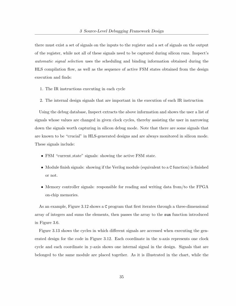
3 Source-Level Debugging Framework Design
there must exist a set of signals on the inputs to the register and a set of signals on the output
of the register, while not all of these signals need to be captured during silicon runs. Inspect’s
automatic signal selection uses the scheduling and binding information obtained during the
HLS compilation flow, as well as the sequence of active FSM states obtained from the design
execution and finds:
1. The IR instructions executing in each cycle
2. The internal design signals that are important in the execution of each IR instruction
Using the debug database, Inspect extracts the above information and shows the user a list of
signals whose values are changed in given clock cycles, thereby assisting the user in narrowing
down the signals worth capturing in silicon debug mode. Note that there are some signals that
are known to be “crucial” in HLS-generated designs and are always monitored in silicon mode.
These signals include:
• FSM “current state” signals: showing the active FSM state.
• Module finish signals: showing if the Verilog module (equivalent to a C function) is finished
or not.
• Memory controller signals: responsible for reading and writing data from/to the FPGA
on-chip memories.
As an example, Figure 3.12 shows a C program that first iterates through a three-dimensional
array of integers and sums the elements, then passes the array to the sum function introduced
in Figure 3.6.
Figure 3.13 shows the cycles in which different signals are accessed when executing the gen-
erated design for the code in Figure 3.12. Each coordinate in the x-axis represents one clock
cycle and each coordinate in y-axis shows one internal signal in the design. Signals that are
belonged to the same module are placed together. As it is illustrated in the chart, while the
35

3 Source-Level Debugging Framework Design
1: int array[2][2][3] = { { {1, 2, 3}, {4, 5, 6} } ,
{ {7, 8, 9}, {10, 11, 12} } };
2: int main() {
3: int result = 0;
4: int a, b, c;
5: for (a = 0; a < 2; a++)
6: for (b = 0; b < 2; b++)
7: for (c = 0; c < 3; c++)
8: result += array[a][b][c];
9: result += sum((int*)array, 12);
10: return result;
11: }
Figure 3.12: An example C program.
Figure 3.13: A chart showing the clock cycles in which every signal is accessed.
36

3 Source-Level Debugging Framework Design
crucial signals are accessed during the entire execution, groups of signals that are local to each
Verilog module (C function) are only accessed when that specific module is executed. This no-
tion is the basis for the automatic signal selection component of the Inspect debugger. Further
explanation on how this information can be extracted is discussed in section 4.2. Having this
information, the automatic signal selection only captures the signals that are changing during
each time window. Finally, after all iterations, all design signals are captured in all of the right
clock cycles. However, changing the list of signals in SignalTap II Logic Analyzer requires a
recompilation of the design which can be time consuming for large designs. The other challenge
in this mode is if the number of capturing signals exceeds the available memory on the FPGA,
causing the process to fail.
When all signal values are captured in the on-chip run mode, the on-chip debug engine
provides the similar feature set that is implemented in the simulation engine using the on-chip
data, meaning the design can be advanced by one clock cycle at a time and any available signal
value in any clock cycle can be obtained. By providing the same interface for both simulation
and on-chip engines, Inspect debugging features implementations remain unchanged in different
debug modes.
It is worth highlighting a key difference in the visibility of data between the simulation and
silicon modes again: In simulation mode, the user can inspect the value of any variable in the
HLS-generated circuit. This is possible as the RTL is being executed in ModelSim and Inspect
can query the simulator to return the value of any logic signal in any particular simulation
cycle. Conversely, in the silicon mode, the user must pre-select signals of interest, subject to
the constraints of limited on-chip block RAM. Only the values of pre-selected signals can be
viewed as the user debugs with Inspect.
To underscore the need for silicon debugging and to explain the reason why functional RTL
simulation is used instead of timing simulation in Inspect, Table 3.1 shows the run-time needed
for functional RTL simulation (zero delay) in comparison to a post-routing timing simulation
for 4 CHStone benchmarks [17]. The CHStone benchmarks are discussed further in Section 6.1.
37

3 Source-Level Debugging Framework Design
Table 3.1: Simulation run-time comparison.
Benchmark RTL Sim (s) Timing Sim (s) Increase (×)
MIPS 0.9 76 84
MOTION 1 118 118
DFMULL 1.6 248 155
DFADD 0.8 37 46
Column 2 shows the run-time, in seconds, for RTL simulation with ModelSim-SE; column 3
shows the run-time for timing simulation; column 4 shows the increase in run-time between RTL
and timing simulation. As illustrated, timing simulation takes roughly 2 orders of magnitude
longer than RTL simulation, and as such, is plainly impractical for large designs with lengthy
vector sets. Furthermore, there are undoubtedly bugs which cannot be discovered even with
a timing simulation, such as timing issues arising from process variations, transient functional
bugs from SEUs, and others. Hence, we feel there is a strong need for HLS debugging strategies
that leverage actual silicon execution, such as those available with Inspect.
3.6 Debugger Features
This section details all the features provided by Inspect. Inspect offers stepping and breakpoints
capabilities that are similar to those found in software debuggers, as well as the ability to watch
variable/signal values and discrepancy detection tools.
3.6.1 Stepping
Two flavours of stepped execution are available to the user, which we call “statement step” and
“cycle step”. Statement step mimics software-like stepping, where the execution is advanced one
C statement at a time. With each statement step, the hardware execution is advanced by one or
more clock cycles until the statement is completed. Cycle step, on the other hand, advances the
hardware execution by a single clock cycle, which is expected to be useful to hardware engineers
38
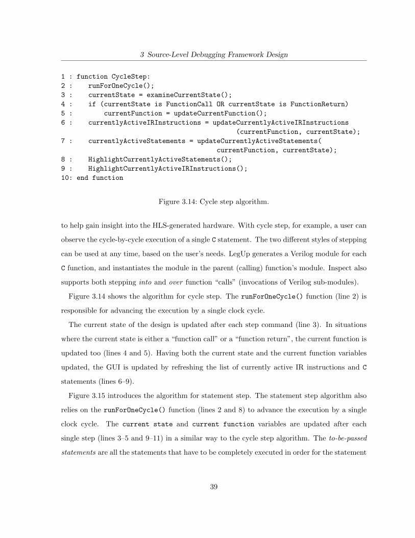
3 Source-Level Debugging Framework Design
1 : function CycleStep:
2 : runForOneCycle();
3 : currentState = examineCurrentState();
4 : if (currentState is FunctionCall OR currentState is FunctionReturn)
5 : currentFunction = updateCurrentFunction();
6 : currentlyActiveIRInstructions = updateCurrentlyActiveIRInstructions
(currentFunction, currentState);
7 : currentlyActiveStatements = updateCurrentlyActiveStatements(
currentFunction, currentState);
8 : HighlightCurrentlyActiveStatements();
9 : HighlightCurrentlyActiveIRInstructions();
10: end function
Figure 3.14: Cycle step algorithm.
to help gain insight into the HLS-generated hardware. With cycle step, for example, a user can
observe the cycle-by-cycle execution of a single C statement. The two different styles of stepping
can be used at any time, based on the user’s needs. LegUp generates a Verilog module for each
C function, and instantiates the module in the parent (calling) function’s module. Inspect also
supports both stepping into and over function “calls” (invocations of Verilog sub-modules).
Figure 3.14 shows the algorithm for cycle step. The runForOneCycle() function (line 2) is
responsible for advancing the execution by a single clock cycle.
The current state of the design is updated after each step command (line 3). In situations
where the current state is either a “function call” or a “function return”, the current function is
updated too (lines 4 and 5). Having both the current state and the current function variables
updated, the GUI is updated by refreshing the list of currently active IR instructions and C
statements (lines 6–9).
Figure 3.15 introduces the algorithm for statement step. The statement step algorithm also
relies on the runForOneCycle() function (lines 2 and 8) to advance the execution by a single
clock cycle. The current state and current function variables are updated after each
single step (lines 3–5 and 9–11) in a similar way to the cycle step algorithm. The to-be-passed
statements are all the statements that have to be completely executed in order for the statement
39
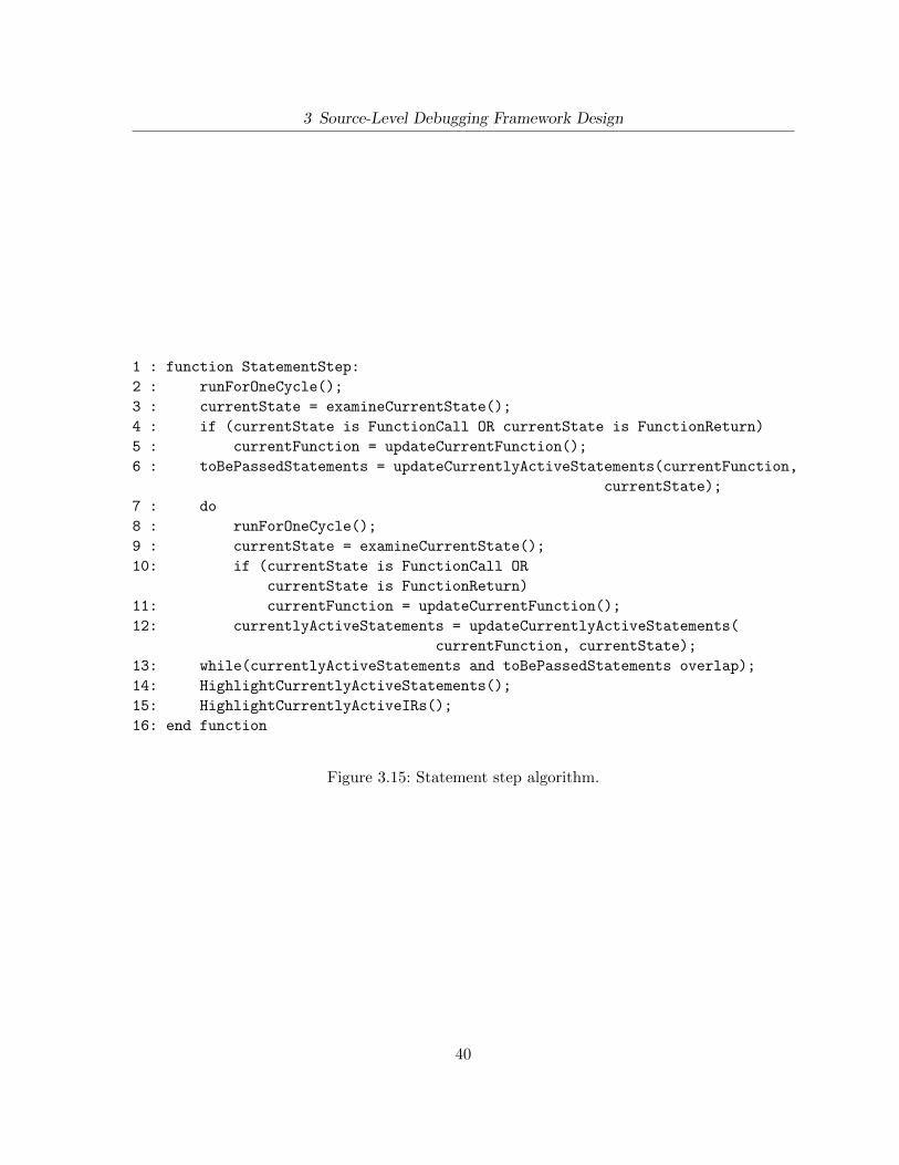
3 Source-Level Debugging Framework Design
1 : function StatementStep:
2 : runForOneCycle();
3 : currentState = examineCurrentState();
4 : if (currentState is FunctionCall OR currentState is FunctionReturn)
5 : currentFunction = updateCurrentFunction();
6 : toBePassedStatements = updateCurrentlyActiveStatements(currentFunction,
currentState);
7 : do
8 : runForOneCycle();
9 : currentState = examineCurrentState();
10: if (currentState is FunctionCall OR
currentState is FunctionReturn)
11: currentFunction = updateCurrentFunction();
12: currentlyActiveStatements = updateCurrentlyActiveStatements(
currentFunction, currentState);
13: while(currentlyActiveStatements and toBePassedStatements overlap);
14: HighlightCurrentlyActiveStatements();
15: HighlightCurrentlyActiveIRs();
16: end function
Figure 3.15: Statement step algorithm.
40
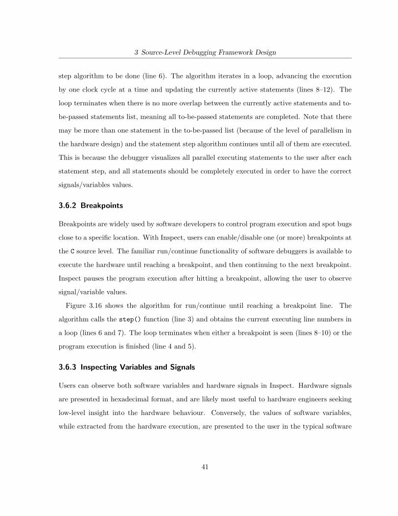
3 Source-Level Debugging Framework Design
step algorithm to be done (line 6). The algorithm iterates in a loop, advancing the execution
by one clock cycle at a time and updating the currently active statements (lines 8–12). The
loop terminates when there is no more overlap between the currently active statements and to-
be-passed statements list, meaning all to-be-passed statements are completed. Note that there
may be more than one statement in the to-be-passed list (because of the level of parallelism in
the hardware design) and the statement step algorithm continues until all of them are executed.
This is because the debugger visualizes all parallel executing statements to the user after each
statement step, and all statements should be completely executed in order to have the correct
signals/variables values.
3.6.2 Breakpoints
Breakpoints are widely used by software developers to control program execution and spot bugs
close to a specific location. With Inspect, users can enable/disable one (or more) breakpoints at
the C source level. The familiar run/continue functionality of software debuggers is available to
execute the hardware until reaching a breakpoint, and then continuing to the next breakpoint.
Inspect pauses the program execution after hitting a breakpoint, allowing the user to observe
signal/variable values.
Figure 3.16 shows the algorithm for run/continue until reaching a breakpoint line. The
algorithm calls the step() function (line 3) and obtains the current executing line numbers in
a loop (lines 6 and 7). The loop terminates when either a breakpoint is seen (lines 8–10) or the
program execution is finished (line 4 and 5).
3.6.3 Inspecting Variables and Signals
Users can observe both software variables and hardware signals in Inspect. Hardware signals
are presented in hexadecimal format, and are likely most useful to hardware engineers seeking
low-level insight into the hardware behaviour. Conversely, the values of software variables,
while extracted from the hardware execution, are presented to the user in the typical software
41
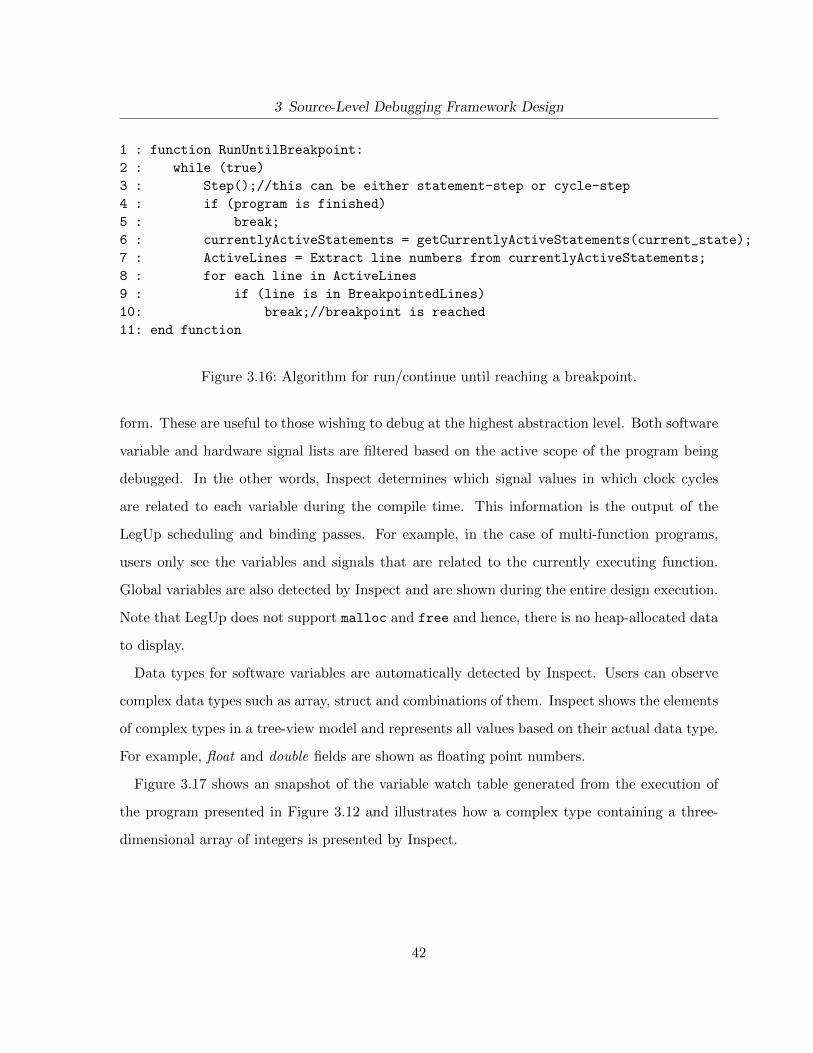
3 Source-Level Debugging Framework Design
1 : function RunUntilBreakpoint:
2 : while (true)
3 : Step();//this can be either statement-step or cycle-step
4 : if (program is finished)
5 : break;
6 : currentlyActiveStatements = getCurrentlyActiveStatements(current_state);
7 : ActiveLines = Extract line numbers from currentlyActiveStatements;
8 : for each line in ActiveLines
9 : if (line is in BreakpointedLines)
10: break;//breakpoint is reached
11: end function
Figure 3.16: Algorithm for run/continue until reaching a breakpoint.
form. These are useful to those wishing to debug at the highest abstraction level. Both software
variable and hardware signal lists are filtered based on the active scope of the program being
debugged. In the other words, Inspect determines which signal values in which clock cycles
are related to each variable during the compile time. This information is the output of the
LegUp scheduling and binding passes. For example, in the case of multi-function programs,
users only see the variables and signals that are related to the currently executing function.
Global variables are also detected by Inspect and are shown during the entire design execution.
Note that LegUp does not support malloc and free and hence, there is no heap-allocated data
to display.
Data types for software variables are automatically detected by Inspect. Users can observe
complex data types such as array, struct and combinations of them. Inspect shows the elements
of complex types in a tree-view model and represents all values based on their actual data type.
For example, float and double fields are shown as floating point numbers.
Figure 3.17 shows an snapshot of the variable watch table generated from the execution of
the program presented in Figure 3.12 and illustrates how a complex type containing a three-
dimensional array of integers is presented by Inspect.
42
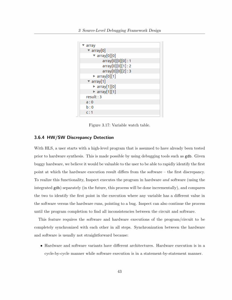
3 Source-Level Debugging Framework Design
Figure 3.17: Variable watch table.
3.6.4 HW/SW Discrepancy Detection
With HLS, a user starts with a high-level program that is assumed to have already been tested
prior to hardware synthesis. This is made possible by using debugging tools such as gdb. Given
buggy hardware, we believe it would be valuable to the user to be able to rapidly identify the first
point at which the hardware execution result differs from the software – the first discrepancy.
To realize this functionality, Inspect executes the program in hardware and software (using the
integrated gdb) separately (in the future, this process will be done incrementally), and compares
the two to identify the first point in the execution where any variable has a different value in
the software versus the hardware runs, pointing to a bug. Inspect can also continue the process
until the program completion to find all inconsistencies between the circuit and software.
This feature requires the software and hardware executions of the program/circuit to be
completely synchronized with each other in all steps. Synchronization between the hardware
and software is usually not straightforward because:
• Hardware and software variants have different architectures. Hardware execution is in a
cycle-by-cycle manner while software execution is in a statement-by-statement manner.
43
3 Source-Level Debugging Framework Design
• Generated hardware designs benefit from parallelism that may completely change the
order of instructions, while keeping the program behaviour correct.
Figure 3.18 introduces the algorithm used by Inspect to synchronize program/circuit execu-
tion and identify the discrepancies. The algorithm works by assuming that debug metadata
information is preserved during the compilation flow and after optimization passes. Therefore,
even though IR instructions execute in parallel during the hardware execution, they will point
to the correct lines in the C code. The algorithm first completes the software and hardware
executions separately and stores variable values in separate containers (lines 5–16). Containers
keep the list of line number and value pairs for each variable (lines 1–3). Each pair includes
the C line number where the value is assigned to the variable, as well as the actual value. The
list of hardware and software values are populated in somewhat different ways. An entry is
added to the hardware list only when the execution reaches an assignment that updates that
specific variable. The UpdatingVariables() function in line 13 accepts the current state of the
design and returns all variables that are updating on that specific state. Conversely, entries are
added to the software list for all live variables after each step command. This creates repetitive
entries in the list of software values which will be handled in the detectBugs() routine. In
fact, this behaviour is because gdb detects the list of program variables but does not provide
any information on “where” in the program the variables may be updated.
The detectBugs() routine finds all discrepancies for each variable between the hardware and
software executions by comparing the list of values obtained from the two different runs. For
each entry in the hardware list, the algorithm attempts to find the first entry in the software
list that has the same line number, and then checks the values (lines 22–28). If values vary, a
bug is found (line 29). In addition, if the end of software list is reached without resolving the
entry in the hardware list, a bug is reported too (lines 32 and 33).
44
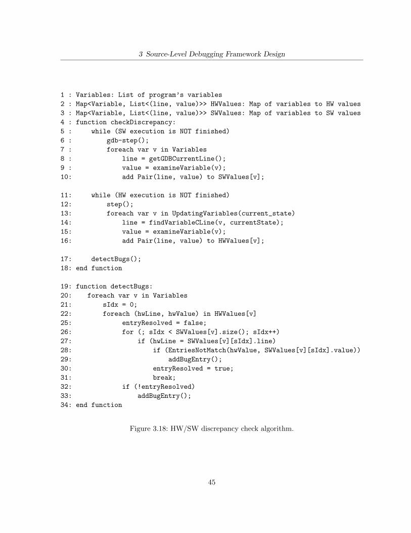
3 Source-Level Debugging Framework Design
1 : Variables: List of program’s variables
2 : Map<Variable, List<(line, value)>> HWValues: Map of variables to HW values
3 : Map<Variable, List<(line, value)>> SWValues: Map of variables to SW values
4 : function checkDiscrepancy:
5 : while (SW execution is NOT finished)
6 : gdb-step();
7 : foreach var v in Variables
8 : line = getGDBCurrentLine();
9 : value = examineVariable(v);
10: add Pair(line, value) to SWValues[v];
11: while (HW execution is NOT finished)
12: step();
13: foreach var v in UpdatingVariables(current_state)
14: line = findVariableCLine(v, currentState);
15: value = examineVariable(v);
16: add Pair(line, value) to HWValues[v];
17: detectBugs();
18: end function
19: function detectBugs:
20: foreach var v in Variables
21: sIdx = 0;
22: foreach (hwLine, hwValue) in HWValues[v]
25: entryResolved = false;
26: for (; sIdx < SWValues[v].size(); sIdx++)
27: if (hwLine = SWValues[v][sIdx].line)
28: if (EntriesNotMatch(hwValue, SWValues[v][sIdx].value))
29: addBugEntry();
30: entryResolved = true;
31: break;
32: if (!entryResolved)
33: addBugEntry();
34: end function
Figure 3.18: HW/SW discrepancy check algorithm.
45

3 Source-Level Debugging Framework Design
3.6.5 RTL/Silicon Discrepancy Detection
In addition to the ability to compare the software execution to RTL simulation described
in Section 3.6.4, Inspect is also capable of comparing the results from a silicon run to RTL
simulation. In this flow, ModelSim and the Signal Tap-instrumented hardware run in tandem,
and the first mismatch between the two is identified. This is useful for cases where bugs occur
only in silicon runs and not in the RTL simulation (e.g. timing related bugs or SEUs). Since the
FSM state is always tracked in silicon mode, Inspect is able to show the user the corresponding
C code at the root of the mismatch.
3.7 Summary
In this chapter, design issues for HLS source-level debugging tools were discussed and the
Inspect debugger framework was introduced. The three levels of abstraction needed for HLS
debugging were described: the C source, the LLVM IR, and the HLS-generated hardware. A
debug database is used to correlate between the related structures in the three abstraction levels.
The Inspect source-level debugger features including stepping, breakpointing, variable/signal
probing, and discrepancy detection tools, were also introduced in this chapter.
46

4 Case Studies
To demonstrate how the Inspect HLS debugger works, this chapter illustrates different Inspect
features using several debugging scenarios that arise in case studies. The C program presented
in Figure 4.1 is used for all case studies throughout this chapter. The program counts the
number of primes in a 3-dimensional array of int. Line 3 declares and initializes the 3D array
as a global variable. Lines 4-16 contain a function, isPrime, that determines if an int type
parameter num is a prime, returning 0 or 1 accordingly. The main function in lines 17-onwards
walks through each element of the array and calls the isPrime function for each, accumulating
the returned values into result, which is ultimately returned by the program.
Inspect offers software-engineer-friendly debugging capabilities for HLS-generated hardware,
as well as offering additional capabilities for those with hardware expertise. Regarding the first
set of capabilities, with Inspect, the user is able to step and execute a program’s C source code,
while behind the scenes (and transparent to the user), the program’s hardware implementation
is executed. Recapping the content from the previous chapter, Inspect offers the following
debugging modes:
• ModelSim simulation debug mode
• Silicon debug mode
• gdb software debug mode
• Automatic bug detection mode
47
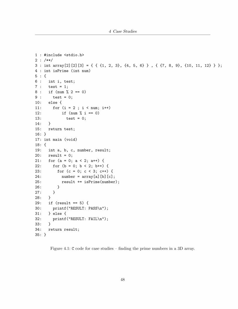
4 Case Studies
1 : #include <stdio.h>
2 : /**/
3 : int array[2][2][3] = { { {1, 2, 3}, {4, 5, 6} } , { {7, 8, 9}, {10, 11, 12} } };
4 : int isPrime (int num)
5 : {
6 : int i, test;
7 : test = 1;
8 : if (num % 2 == 0)
9 : test = 0;
10: else {
11: for (i = 2 ; i < num; i++)
12: if (num % i == 0)
13: test = 0;
14: }
15: return test;
16: }
17: int main (void)
18: {
19: int a, b, c, number, result;
20: result = 0;
21: for (a = 0; a < 2; a++) {
22: for (b = 0; b < 2; b++) {
23: for (c = 0; c < 3; c++) {
24: number = array[a][b][c];
25: result += isPrime(number);
26: }
27: }
28: }
29: if (result == 5) {
30: printf("RESULT: PASS\n");
31: } else {
32: printf("RESULT: FAIL\n");
33: }
34: return result;
35: }
Figure 4.1: C code for case studies – finding the prime numbers in a 3D array.
48
4 Case Studies
4.1 ModelSim Simulation Debug Mode
The auto-generated Verilog design of the input C program is simulated by ModelSim in this
mode. Users are able to see the three basic view panels (source-code, IR, Verilog) as well as
the watch table for hardware signals and software variables. The following actions should be
taken to start ModelSim simulation debug:
1. Open the TCP connection to the ModelSim process by clicking File → Open Connec-
tion menu item.
2. Load the Verilog design file and all required libraries in ModelSim by clicking File →
Load Design menu item.
3. Set the desired stepping mode by selecting the Cycle Step or Statement Step option
and start the debug process by clicking on Step button on top of the main window.
4.1.1 Case Study
In this case study, the Verilog design is first generated for the given C program presented in
Figure 4.1. By following the instructions to start the debug process, users are able to advance
the circuit/program execution, observe the program execution and watch variable/signal values
from both software and hardware perspectives. Figure 4.2 shows the Inspect GUI during the
debug session for the given example. Labels 1©, 2©, and 3© illustrate the C source, IR, and
Verilog views respectively. Code highlighting shows actively executing C statements and IR
instructions. Observe that, since LegUp directly synthesizes the LLVM IR, the FSM state for
each IR instruction is displayed in the IR window, giving insight into the hardware, specifically
the scheduling results of HLS. In the debug session, the hardware is in FSM state #13 (also
displayed at label 4©). By clicking on any IR instruction, the related Verilog code parts are
shown to the user. Observe in the panel labeled 3© that the hardware is currently performing
an integer comparison – the corresponding line of Verilog is shown. Highlighting in the panels
49

4 Case Studies
Figure 4.2: Inspect GUI during ModelSim simulation debug.
labeled 1© and 2© illustrate that presently, the hardware is computing the comparison in the
inner-most loop.
C variables and their most recent values are shown in panel labeled 6© and hardware signal
values that are updated in the current state of the design are shown in panel labeled 7©.
Users can select from the two available flavours of stepping in this mode as discussed in
Section 3.6 (label 5©). By selecting the Statement Step radio button, the design advances to
the next statement from the C code perspective, anytime the stepping command is issued. The
Cycle Step radio button changes this behaviour and only advances the program by one clock
cycle from the hardware perspective.
By default, cycle step mode behaves as Step-In with respect to function calls, meaning that
the debugger enters the called function. Users can change this behaviour to Step-Over by
50
4 Case Studies
selecting statement step mode when a call statement is reached.
Breakpoints can be set at any line that contains executable statement by clicking on the line
number in left side of the C code panel. The Run/Continue button can be used to run the
program until a breakpointed line is reached.
4.2 Silicon Debug Mode
Inspect’s silicon debug mode executes the design in silicon on the FPGA. The Inspect debugger
presently supports the Altera Cyclone IV FPGA family [5]. The debugging process for this
mode starts by clicking on the File → Run Silicon menu item. The following parameters
should be set by users when this mode is used:
• Silicon debug window size: defines the number of cycles for which Inspect attempts to
capture signal values. This window-based debug procedure was discussed in Section 3.5.2.
It should be noted that a small window size causes Inspect to take much more time to finish
debugging the design, while a large window size may result in an execution failure, due
to limited on-chip memory on FPGAs. This parameter should be set with consideration
for design size and the FPGA available memory.
• Automatic signal selection: enabling this option allows Inspect to change the list of
observed signals after each silicon run iteration. This is performed using the algorithm
discussed in Section 3.5.2.
Figure 4.3 shows the automatic signal selection window of Inspect for the example in
Figure 4.2. Signals are presented in the left side of the window, and green cells show the
clock cycles where each signal is read from or written to. An estimation of the number
of unique LegUp FSM states and the total number of clock cycles for which each signal
is accessed through the entire run, is shown in the parentheses after each signal name.
These two numbers can be different. For example, the signal main 10 12 is accessed in one
LegUp FSM state, but in sixteen different clock cycles (the FSM state is inside a nested
51
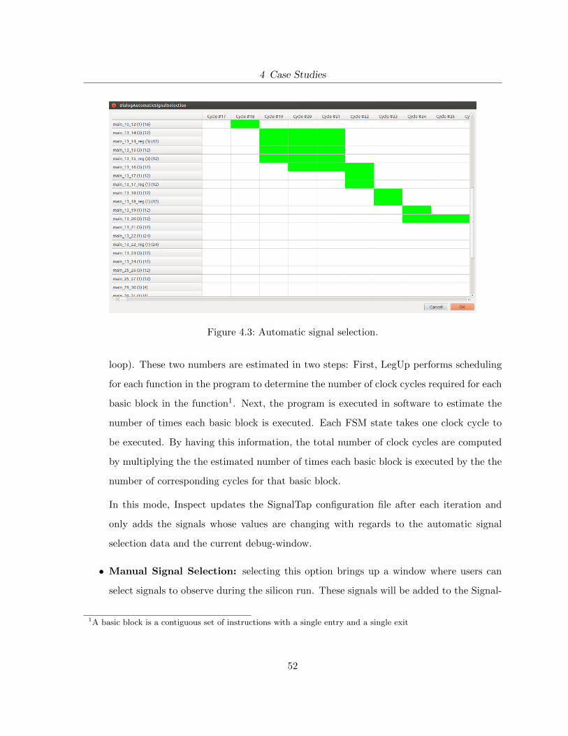
4 Case Studies
Figure 4.3: Automatic signal selection.
loop). These two numbers are estimated in two steps: First, LegUp performs scheduling
for each function in the program to determine the number of clock cycles required for each
basic block in the function1. Next, the program is executed in software to estimate the
number of times each basic block is executed. Each FSM state takes one clock cycle to
be executed. By having this information, the total number of clock cycles are computed
by multiplying the the estimated number of times each basic block is executed by the the
number of corresponding cycles for that basic block.
In this mode, Inspect updates the SignalTap configuration file after each iteration and
only adds the signals whose values are changing with regards to the automatic signal
selection data and the current debug-window.
• Manual Signal Selection: selecting this option brings up a window where users can
select signals to observe during the silicon run. These signals will be added to the Signal-
1A basic block is a contiguous set of instructions with a single entry and a single exit
52
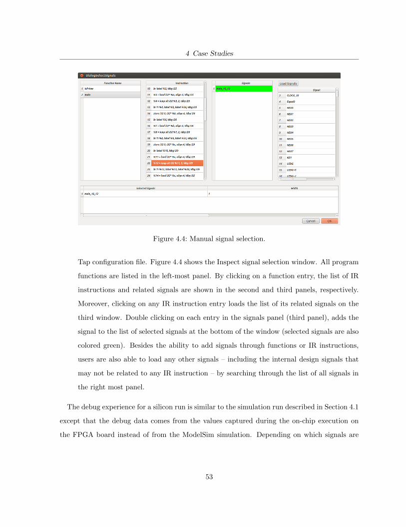
4 Case Studies
Figure 4.4: Manual signal selection.
Tap configuration file. Figure 4.4 shows the Inspect signal selection window. All program
functions are listed in the left-most panel. By clicking on a function entry, the list of IR
instructions and related signals are shown in the second and third panels, respectively.
Moreover, clicking on any IR instruction entry loads the list of its related signals on the
third window. Double clicking on each entry in the signals panel (third panel), adds the
signal to the list of selected signals at the bottom of the window (selected signals are also
colored green). Besides the ability to add signals through functions or IR instructions,
users are also able to load any other signals – including the internal design signals that
may not be related to any IR instruction – by searching through the list of all signals in
the right most panel.
The debug experience for a silicon run is similar to the simulation run described in Section 4.1
except that the debug data comes from the values captured during the on-chip execution on
the FPGA board instead of from the ModelSim simulation. Depending on which signals are
53
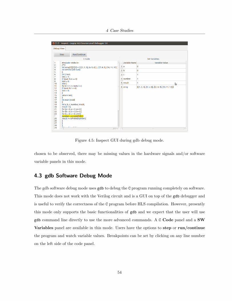
4 Case Studies
Figure 4.5: Inspect GUI during gdb debug mode.
chosen to be observed, there may be missing values in the hardware signals and/or software
variable panels in this mode.
4.3 gdb Software Debug Mode
The gdb software debug mode uses gdb to debug the C program running completely on software.
This mode does not work with the Verilog circuit and is a GUI on top of the gdb debugger and
is useful to verify the correctness of the C program before HLS compilation. However, presently
this mode only supports the basic functionalities of gdb and we expect that the user will use
gdb command line directly to use the more advanced commands. A C Code panel and a SW
Variables panel are available in this mode. Users have the options to step or run/continue
the program and watch variable values. Breakpoints can be set by clicking on any line number
on the left side of the code panel.
54

4 Case Studies
Figure 4.6: The changed part of the Verilog file with the injected bug.
4.3.1 Case Study
Figure 4.5 shows a snapshot from the debug process in this mode. The current executing C
statement is highlighted and variable values are shown in the watch panel. A breakpoint is also
set at line 24.
The default behaviour of the debugger in this mode is to step-in through all function calls.
When the program is complete, the returned value is shown in the watch panel.
4.4 Automatic Bug Detection Mode
This mode is dedicated to detect discrepancies between the hardware and software executions
of the program/circuit. Bug detection is automatic, meaning it is performed without user’s
interaction. The detected discrepancies can be observed by navigating to the Discrepancy
Log panel in the main window. Each discrepancy record contains the variable name as well as
the software value, related line number in the C code and hardware value fields. The number
of discrepancies is also shown in the status bar, at the bottom of the main window.
4.4.1 Case Study
To illustrate this mode, we inserted a bug into the Verilog generated by LegUp. Figure 4.6
shows the altered part of the Verilog code. An integer value of 3 is changed to 2 in a Verilog
comparison. The change is related to the statement c < 3 at line number 23 of the C code and
it causes the program to iterate two times (instead of three times) in the inner most loop.
Figure 4.7 shows the number of discrepancies that are found after the proposed bug is injected.
55
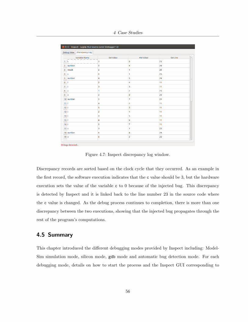
4 Case Studies
Figure 4.7: Inspect discrepancy log window.
Discrepancy records are sorted based on the clock cycle that they occurred. As an example in
the first record, the software execution indicates that the c value should be 3, but the hardware
execution sets the value of the variable c to 0 because of the injected bug. This discrepancy
is detected by Inspect and it is linked back to the line number 23 in the source code where
the c value is changed. As the debug process continues to completion, there is more than one
discrepancy between the two executions, showing that the injected bug propagates through the
rest of the program’s computations.
4.5 Summary
This chapter introduced the different debugging modes provided by Inspect including: Model-
Sim simulation mode, silicon mode, gdb mode and automatic bug detection mode. For each
debugging mode, details on how to start the process and the Inspect GUI corresponding to
56

4 Case Studies
each mode were described. Case studies were also presented to show Inspect’s behaviour in the
different modes.
57
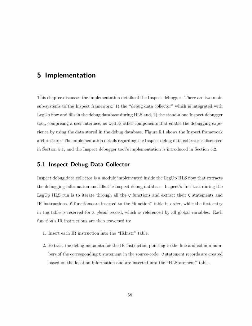
5 Implementation
This chapter discusses the implementation details of the Inspect debugger. There are two main
sub-systems to the Inspect framework: 1) the “debug data collector” which is integrated with
LegUp flow and fills in the debug database during HLS and, 2) the stand-alone Inspect debugger
tool, comprising a user interface, as well as other components that enable the debugging expe-
rience by using the data stored in the debug database. Figure 5.1 shows the Inspect framework
architecture. The implementation details regarding the Inspect debug data collector is discussed
in Section 5.1, and the Inspect debugger tool’s implementation is introduced in Section 5.2.
5.1 Inspect Debug Data Collector
Inspect debug data collector is a module implemented inside the LegUp HLS flow that extracts
the debugging information and fills the Inspect debug database. Inspect’s first task during the
LegUp HLS run is to iterate through all the C functions and extract their C statements and
IR instructions. C functions are inserted to the “function” table in order, while the first entry
in the table is reserved for a global record, which is referenced by all global variables. Each
function’s IR instructions are then traversed to:
1. Insert each IR instruction into the “IRInstr” table.
2. Extract the debug metadata for the IR instruction pointing to the line and column num-
bers of the corresponding C statement in the source-code. C statement records are created
based on the location information and are inserted into the “HLStatement” table.
58
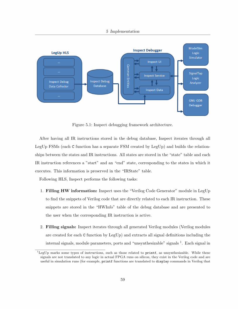
5 Implementation
Figure 5.1: Inspect debugging framework architecture.
After having all IR instructions stored in the debug database, Inspect iterates through all
LegUp FSMs (each C function has a separate FSM created by LegUp) and builds the relation-
ships between the states and IR instructions. All states are stored in the “state” table and each
IR instruction references a ”start” and an “end” state, corresponding to the states in which it
executes. This information is preserved in the “IRState” table.
Following HLS, Inspect performs the following tasks:
1. Filling HW information: Inspect uses the “Verilog Code Generator” module in LegUp
to find the snippets of Verilog code that are directly related to each IR instruction. These
snippets are stored in the “HWInfo” table of the debug database and are presented to
the user when the corresponding IR instruction is active.
2. Filling signals: Inspect iterates through all generated Verilog modules (Verilog modules
are created for each C function by LegUp) and extracts all signal definitions including the
internal signals, module parameters, ports and “unsynthesizable” signals 1. Each signal in
1LegUp marks some types of instructions, such as those related to printf, as unsynthesizable. While thesesignals are not translated to any logic in actual FPGA runs on silicon, they exist in the Verilog code and areuseful in simulation runs (for example, printf functions are translated to display commands in Verilog that
59

5 Implementation
the LegUp-generated design is related to an IR instruction. This relationship is captured
by Inspect and is stored in the “InstructionSignal” table of the debug database.
3. Filling variables: LegUp creates dual-port RAM module instances for all variables in
the code. Each RAM instance has a unique tag number (which is used for addressing
purposes) and a pre-defined size in bytes. It should be noted that presently LegUp does
not support dynamic allocation and therefore, all C variable have a deterministic size
at compile time. Inspect iterates through all the LegUp-generated RAM instances and
creates records in the “variable” table of the debug database, storing the tag number and
variable name for each RAM instance, as well as other information regarding the type of
the variables. Variable types are stored in a hierarchical way, with each hierarchy having
its own size and element numbers. For example, a three-dimensional array of integers with
dimensions being 2, 3 and 2 (int[2][3][2]) is represented by a top hierarchy having two
entries, were each is two-dimensional array of 3 and 2. The hierarchy goes down until
reaching the primitive data types (int, float and double) which have only one element
and a pre-defined size in bytes. Inspect also extracts the initialization values for global
variables (if any exists) and stores them in the “variable data” table of the debug database.
The Inspect debug data collector does not interfere with LegUp HLS algorithms and only
collects information when it is enabled. The Inspect debug data collector requires some LegUp
compilation flags (NO OPT2, NO INLINE3), as well as LLVM debugging flag (-g parameter4) to
be turned on in order to work properly.
5.2 Inspect Debugger
The Inspect debugger tool is a stand-alone application that enables the debugging experience
by accessing the information in the debug database. Inspect debugger tool’s components are:
actually display the values in ModelSim simulation runs).2NO OPT sets the compiler to compile the program with all optimizations turned off (-O0).3NO INLINE sets the compiler to not apply inlining for functions that are defined as inline.4-g parameter sets the compiler to generate source-level debug metadata during the compilation.
60

5 Implementation
• Inspect UI component
• Inspect service component
• Database component
• Common entities (data model)
5.3 Inspect UI
The Inspect UI component includes all routines and definitions to present the user interface and
visualize the behaviour of the debugger. The UI component is built in the Qt framework [24]
and it connects to the Inspect service component in order to obtain the information to show
the user. All forms, windows and interfaces of the UI component were presented via the case
studies in Chapter 4.
5.4 Inspect Service Component
The Inspect service component contains all routines and procedures required to implement the
debugging features. All of the algorithms introduced in Chapter 3, as well as the integration
with external systems (ModelSim, SignalTap and gdb) are implemented in this component. The
most important modules of the Inspect service component are described below.
5.4.1 ModelSim Integration
ModelSim integration is accomplished by running a tcl script in a live ModelSim process.
The script listens on a TCP port for specific commands to pass to the ModelSim process. The
Inspect debugger establishes a TCP connection to ModelSim and sends commands to control the
design’s simulation progress. By default, the tcl script is set to listen for incoming connections
on TCP port 2000.
List of ModelSim commands that are presently used by Inspect are as follows:
61
5 Implementation
• vlib, vlog and vsim: used to create the design library and the working directory, compile
the Verilog source code, and invoke the ModelSim simulator.
• run: used to advance the simulation by a specific amount of time (usually one clock
cycle).
• examine: used to examine the design’s signal values.
The current framework can be extended to support the feature of setting variables/signals
values during the simulation debug in the future.
5.4.2 SignalTap Integration
Inspect uses the Altera SignalTap II Logic Analyzer in order to perform on-chip debug and
capture signal values during the silicon run. The list of signals to be examined, as well as
the capturing window information and other necessary debugging parameters are passed to the
SignalTap process in the form of SignalTap STP files. The Inspect service component accepts
the list of signals from the UI component and automatically creates the STP files and includes
it in the Quartus project file initially created by LegUp for on-chip debug purposes.
By attaching the STP files to the Quartus project file and performing the required compilation
flows in Quartus, SignalTap captures the signal values for the specified time-window and stores
the data in output CSV files. The Inspect service component also includes a CSV parser module
that parses the SignalTap-generated CSV files and extracts all signals and their corresponding
values in different clock cycles.
5.4.3 gdb Integration
Inspect’s gdb module is designed to bring gdb functionality to the framework. It connects to
the gdb debugger through the gdb/MI interface by using the libmigdb library [21]. The current
usage of gdb within Inspect is capable of:
• Stepping the program’s execution.
62

5 Implementation
• Examining variables including all local and global variables in the program.
• Keeping track of the program’s stack frame to find the current active scope of the program.
• Changing stack frames.
The gdb module is used in different parts of the framework, such as the discrepancy detection
tool and Inspect’s pure gdb debug mode.
5.5 Database Access
The Inspect debug database is implemented using the MySQL database management sys-
tem [29]. The debug database is filled by the Inspect debug data collector module during
the LegUp HLS run. Filling out the debug database may cause time overheads during the
HLS compilation flow, but by using the database management system Inspect is able to build
the debug data for the given program at the first compilation and preserve it for further uses.
Moreover, the database solution provides a better scalability and management compared to
other in-memory or file-based solutions. The database component of the Inspect debugger tool
provides the extensive set of functions to load any form of information from the debug database.
The database component is the only part of the debugger tool that has direct access to the
debug database and all components pass their data-related requests to this component. All
entities in the debug database are given a unique auto-incremented identification number by
the debug data module during the HLS run. These IDs can be fetched by the Inspect service
component and used to obtain more information about each entity by passing the suitable
ID as the parameter. The following is a list of all routines provided by the Inspect database
component:
• IR instruction routines: Contains methods to load IR instructions by: 1) a source-level
C line number, 2) LegUp FSM state number, 3) a unique identification number (ID).
63

5 Implementation
• High-level statement routines: Contains methods to load individual or all high-level
statements.
• HW signal routines: Contains methods to load HW signal entities by their name or
ID.
• LegUp FSM routines: Contains methods to load FSM states, as well as finding the
corresponding start and end states for IR instruction records.
• Function routines: Contains methods to load all function entities from the database.
• Variable routines: Contains methods to load all variable entities from the database as
well as the information about variable data types and initial data.
The SQL script used to generate the schema for Inspect debug database is presented in
Appendix A.
5.6 Common Entities
The common entities component of the Inspect debugger tool contains all classes and definitions
that are used throughout the application. Entities in this layer include class definitions for
functions, high-level statements, IR instructions, FSM states, variables, variable types and HW
signals, as well as some common utility functions. These entity definitions have a one-to-one
correspondence with data records in the SQL database and are used to represent the debug
database information at run-time. All necessary containers and a list of entities that are used
by all system components are created in a global scope. The database component fills in the
containers with the information from the database when the application starts and all other
components use the information in order to perform their tasks.
64

5 Implementation
5.7 Summary
Implementation details for the Inspect debugger’s main components were discussed in this
chapter. First, the Inspect debug data collector module that fills the debug database during
the HLS run was discussed. Next, the Inspect debugger tool and all of its components including
its integration to external tools (ModelSim, SignalTap and gdb) were discussed.
65

6 Experimental Results
As with any research on debugging, it is difficult to numerically quantify the productivity im-
provements arising from new methodologies, such as those enabled by Inspect. In this chapter,
an experimental study of the automated bug discrepancy detection is presented. To achieve
this, the automated discrepancy detection algorithm is applied on several buggy designs and the
number of cycles that it takes for the tool to detect discrepancies are reported. This chapter’s
experiments are:
• Software versus RTL simulation discrepancy detection
• Circuit RTL simulation versus silicon discrepancy detection
As the first experiment, 6 of the CHStone benchmarks [17] are selected. The benchmarks
characteristics are discussed further in Section 6.1. The selected benchmarks were synthesized
using the LegUp 3.0 HLS flow and 6 functionally correct solutions were created. Three buggy
variants for each benchmark were then created, producing 18 buggy Verilog implementations
in total to test the system with. All bugs are injected to the generated Verilog file for each
benchmark. Bugs are tried to be diverse and cover many aspects of the benchmarks, including:
changing variable values, operations, control flow and function calls. More details about the
injected bugs for each benchmark are described in the subsequent sections. Note that the CH-
Stone circuits have built-in input vectors and incorporate correctness checking of the computed
results versus golden outputs. Thus, we can “execute” the circuits and their correctness is
assessed as part of the circuit itself.
66
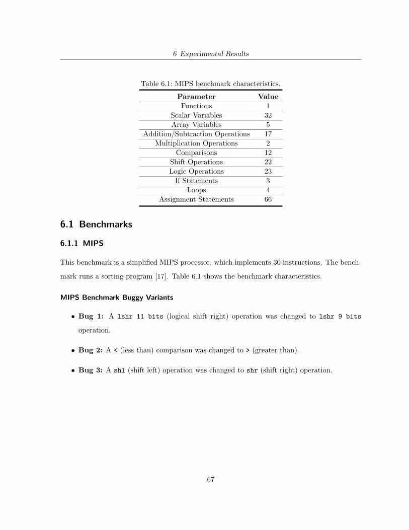
6 Experimental Results
Table 6.1: MIPS benchmark characteristics.
Parameter Value
Functions 1
Scalar Variables 32
Array Variables 5
Addition/Subtraction Operations 17
Multiplication Operations 2
Comparisons 12
Shift Operations 22
Logic Operations 23
If Statements 3
Loops 4
Assignment Statements 66
6.1 Benchmarks
6.1.1 MIPS
This benchmark is a simplified MIPS processor, which implements 30 instructions. The bench-
mark runs a sorting program [17]. Table 6.1 shows the benchmark characteristics.
MIPS Benchmark Buggy Variants
• Bug 1: A lshr 11 bits (logical shift right) operation was changed to lshr 9 bits
operation.
• Bug 2: A < (less than) comparison was changed to > (greater than).
• Bug 3: A shl (shift left) operation was changed to shr (shift right) operation.
67
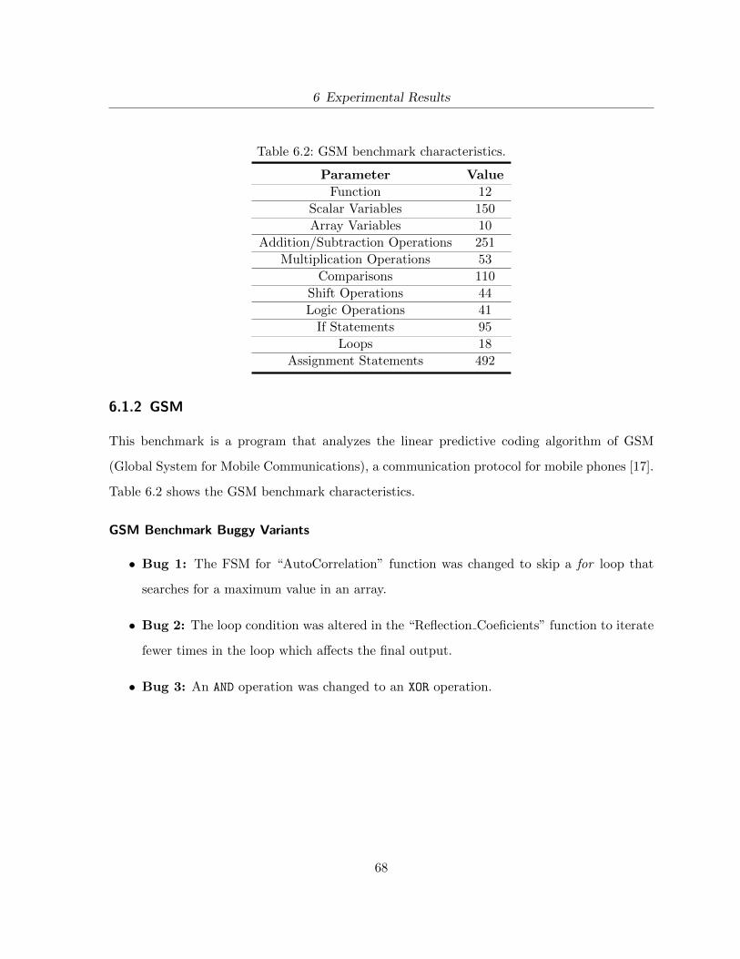
6 Experimental Results
Table 6.2: GSM benchmark characteristics.
Parameter Value
Function 12
Scalar Variables 150
Array Variables 10
Addition/Subtraction Operations 251
Multiplication Operations 53
Comparisons 110
Shift Operations 44
Logic Operations 41
If Statements 95
Loops 18
Assignment Statements 492
6.1.2 GSM
This benchmark is a program that analyzes the linear predictive coding algorithm of GSM
(Global System for Mobile Communications), a communication protocol for mobile phones [17].
Table 6.2 shows the GSM benchmark characteristics.
GSM Benchmark Buggy Variants
• Bug 1: The FSM for “AutoCorrelation” function was changed to skip a for loop that
searches for a maximum value in an array.
• Bug 2: The loop condition was altered in the “Reflection Coeficients” function to iterate
fewer times in the loop which affects the final output.
• Bug 3: An AND operation was changed to an XOR operation.
68

6 Experimental Results
Table 6.3: Motion benchmark characteristics.
Parameter Value
Function 13
Scalar Variables 146
Array Variables 12
Addition/Subtraction Operations 299
Multiplication Operations -
Comparisons 155
Shift Operations 127
Logic Operations 55
If Statements 115
Loops 71
Assignment Statements 1100
6.1.3 MOTION
This is a benchmark that decodes a motion vector in MPEG-2 format, an audio/video decom-
pression method [17]. Table 6.3 shows the characteristics of the Motion benchmark.
MOTION Benchmark Buggy Variants
• Bug 1: The FSM was changed in the “motion vectors” function to skip the if block of
an if-else block such that the else block is always executed.
• Bug 2: The constant value of 32′d1 was changed to 32′d10 in the “decode motion vector”
function.
• Bug 3: The >>> (arithmetic shift right) operation was changed to <<< (arithmetic shift
left) operation in “get motion code” function.
69

6 Experimental Results
Table 6.4: DFMUL benchmark characteristics.
Parameter Value
Function 16
Scalar Variables 92
Array Variables 4
Addition/Subtraction Operations 28
Multiplication Operations 4
Comparisons 34
Shift Operations 41
Logic Operations 61
If Statements 38
Loops 1
Assignment Statements 159
6.1.4 DFMUL
This benchmark is a program that implements IEC/IEEE-standard double-precision floating
point multiplication. The program uses 64-bit integer numbers [17]. Table 6.4 shows the
DFMUL’s characteristics.
DFMUL Benchmark Buggy Variants
• Bug 1: The memory controller input signal was changed in the “float64 is nan” function.
The changed value is passed to another function as an argument.
• Bug 2: The FSM transition was changed in order to reverse the effect of an if-else
condition block.
• Bug 3: A bitwise OR operation was changed to a bitwise AND operation in the “float64 mul”
function.
70
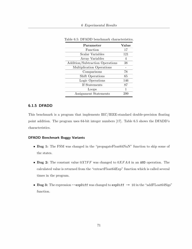
6 Experimental Results
Table 6.5: DFADD benchmark characteristics.
Parameter Value
Function 17
Scalar Variables 121
Array Variables 4
Addition/Subtraction Operations 38
Multiplication Operations -
Comparisons 78
Shift Operations 65
Logic Operations 146
If Statements 87
Loops 1
Assignment Statements 299
6.1.5 DFADD
This benchmark is a program that implements IEC/IEEE-standard double-precision floating
point addition. The program uses 64-bit integer numbers [17]. Table 6.5 shows the DFADD’s
characteristics.
DFADD Benchmark Buggy Variants
• Bug 1: The FSM was changed in the “propagateFloat64NaN” function to skip some of
the states.
• Bug 2: The constant value 0X7FF was changed to 0XFAA in an AND operation. The
calculated value is returned from the “extractFloat64Exp” function which is called several
times in the program.
• Bug 3: The expression --expDiff was changed to expDiff -= 10 in the “addFLoat64Sigs”
function.
71
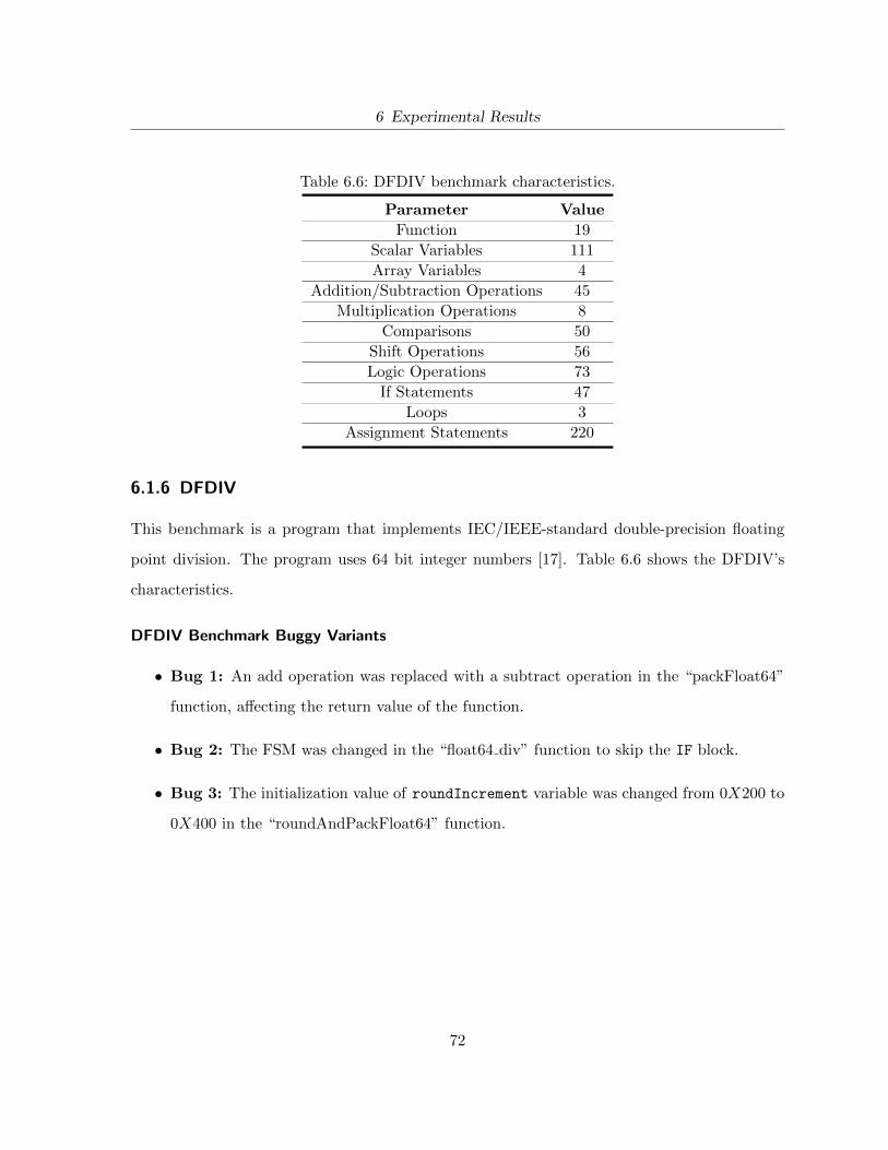
6 Experimental Results
Table 6.6: DFDIV benchmark characteristics.
Parameter Value
Function 19
Scalar Variables 111
Array Variables 4
Addition/Subtraction Operations 45
Multiplication Operations 8
Comparisons 50
Shift Operations 56
Logic Operations 73
If Statements 47
Loops 3
Assignment Statements 220
6.1.6 DFDIV
This benchmark is a program that implements IEC/IEEE-standard double-precision floating
point division. The program uses 64 bit integer numbers [17]. Table 6.6 shows the DFDIV’s
characteristics.
DFDIV Benchmark Buggy Variants
• Bug 1: An add operation was replaced with a subtract operation in the “packFloat64”
function, affecting the return value of the function.
• Bug 2: The FSM was changed in the “float64 div” function to skip the IF block.
• Bug 3: The initialization value of roundIncrement variable was changed from 0X200 to
0X400 in the “roundAndPackFloat64” function.
72
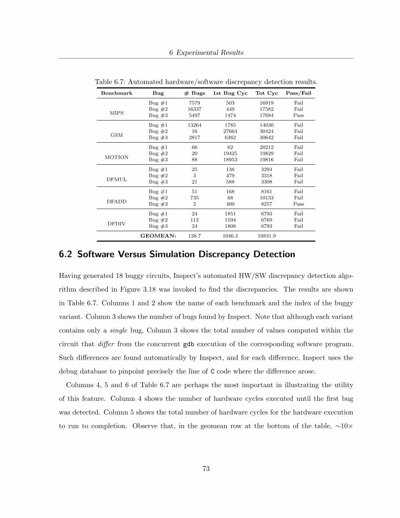
6 Experimental Results
Table 6.7: Automated hardware/software discrepancy detection results.
Benchmark Bug # Bugs 1st Bug Cyc Tot Cyc Pass/Fail
MIPS
Bug #1 7579 503 16919 FailBug #2 16337 449 17582 FailBug #3 5497 1474 17684 Pass
GSM
Bug #1 13264 1785 14030 FailBug #2 16 27664 30424 FailBug #3 2817 6362 30642 Fail
MOTION
Bug #1 66 62 20212 FailBug #2 20 19425 19829 FailBug #3 88 18953 19816 Fail
DFMUL
Bug #1 25 138 3294 FailBug #2 3 479 3318 FailBug #3 21 588 3308 Fail
DFADD
Bug #1 51 168 8161 FailBug #2 735 68 10133 FailBug #3 2 400 8257 Pass
DFDIV
Bug #1 24 1851 6793 FailBug #2 112 1594 6769 FailBug #3 24 1808 6793 Fail
GEOMEAN: 138.7 1046.4 10831.9
6.2 Software Versus Simulation Discrepancy Detection
Having generated 18 buggy circuits, Inspect’s automated HW/SW discrepancy detection algo-
rithm described in Figure 3.18 was invoked to find the discrepancies. The results are shown
in Table 6.7. Columns 1 and 2 show the name of each benchmark and the index of the buggy
variant. Column 3 shows the number of bugs found by Inspect. Note that although each variant
contains only a single bug, Column 3 shows the total number of values computed within the
circuit that differ from the concurrent gdb execution of the corresponding software program.
Such differences are found automatically by Inspect, and for each difference, Inspect uses the
debug database to pinpoint precisely the line of C code where the difference arose.
Columns 4, 5 and 6 of Table 6.7 are perhaps the most important in illustrating the utility
of this feature. Column 4 shows the number of hardware cycles executed until the first bug
was detected. Column 5 shows the total number of hardware cycles for the hardware execution
to run to completion. Observe that, in the geomean row at the bottom of the table, ∼10×
73
6 Experimental Results
fewer cycles (on average) are executed to detect the first bug vs. completing the execution.
For each bug, the user is shown the precise line of C code where the mismatch occurred. By
knowing the C line where the problem arises, users can put a breakpoint on the line and closely
follow the hardware execution (observing signal values and relating them to IR and source-level
concepts) in order to fix the problem. However, currently this may need some hardware skills.
A future work direction for the Inspect framework is to extend this functionality to propose
bug fix suggestions to users with no hardware design skills.
It is expected that, without Inspect, a traditional debugging cycle would operate as follows:
1. First, the user would execute the design to completion and check for an error in the overall
circuit outputs.
2. Finding such an error, the user would begin backtracking to narrow down the source of
the error, likely by adding $display statements into the Verilog code.
3. Multiple tedious manual modifications of the HLS-generated Verilog would be needed,
along with associated hardware executions until the precise location of the bug was found.
4. Once the line of Verilog code where the bug originated is found, the user would need to
understand the HLS-generated Verilog in order to locate the bug from the C perspective.
Column 6 shows that for 16 of 18 cases, the bug did indeed propagate to overall circuit
outputs – such cases failed correctness checking. However, for 2 of the cases, the bug caused
incorrect intermediate values, but those values did not propagate to overall outputs, likely
because the built-in test vectors for CHStone did not exercise certain portions of the circuit.
Thus, the user would most likely presume (incorrectly) that such circuits were bug free. Such
bugs were nevertheless uncovered with Inspect, which is believed as a significant advantage of
Inspect vs. manual methods.
74

6 Experimental Results
6.3 RTL Simulation Versus Silicon Run Discrepancy Detection
In the second experiment, Inspect’s silicon debug mode is evaluated. Three different bugs
are injected into the LegUp-generated FSM of 4 benchmarks, creating total of 12 buggy pro-
grams. Each bug consists of changing one or more transitions in the FSM state diagram.
Sections 6.3.1, 6.3.2, 6.3.3 and 6.3.4 introduce the buggy circuits for this experiment.
6.3.1 MIPS Benchmark Bugs
• Bug 1: Changed the destination state of a transition.
• Bug 2: Reversed the state destinations corresponding to an if-else block.
• Bug 3: Skipped over a state that impacted a return value computed by a Verilog module.
6.3.2 MOTION Benchmark Bugs
• Bug 1: Changed a transition of the FSM in the “motion vectors” function to skip the
if block of an if-else block and always execute the else block.
• Bug 2: Removed a function call (“initialize Buffer”) and jumped to the next state.
• Bug 3: Reversed the state destinations corresponding to an if-else block in the “mo-
tion vectors” function.
6.3.3 DFMUL Benchmark Bugs
• Bug 1: Changed the destination state of a transition in the “float64 mul” function.
• Bug 2: Changed the destination state of a transition which caused a halt in a function
call.
• Bug 3: Changed a transition of the FSM in the ‘float64 mul” function to skip the if
block of an if-else block and always execute the else block.
75
6 Experimental Results
6.3.4 DFADD Benchmark Bugs
• Bug 1: Changed the destination state of a transition in the “packFloat64” function. This
introduced an infinite loop in the program.
• Bug 2: Changed the destination state of a transition.
• Bug 3: Changed the destination state of a jump branch transition in the “addFloat64Sigs”
function.
Inspect’s silicon mode was used to find the bug in the FSM for all the buggy circuits. This
experiment reflects the scenario where Quartus II introduced bugs during synthesis/place/route,
or where the bugs are within the silicon itself. The current FSM state (in all FSMs) is specified
as being among the hardware signals to observe in Signal Tap. For this experiment, Inspect is
set to trace in windows of 2000 cycles, meaning that, the Cyclone IV device [5] is configured to
capture the FSM state for 2000 cycles (via Signal Tap), adjust the Signal Tap trigger condition,
reconfigure the Cyclone IV device, capture the FSM state for the next 2000 cycles, and so
on. For each window, Inspect automatically compares the sequence of FSM states extracted
from the silicon, with those extracted from the circuit’s RTL simulation in ModelSim. When
a discrepancy is found, Inspect uses the debug database to point the user to the line of C code
related to the faulty state.
The results for the silicon debugging experiment are shown in Table 6.8. Column 3 shows the
cycle number at which the first bug was detected; column 4 shows the total number of cycles for
hardware execution to complete. Column 5 indicates whether the design passed or failed the
built-in correctness checking. The time required for debugging is closely tied with the number
of device reconfigurations required – this is shown in parentheses in columns 3 and 4. Observe
that for 7/12 cases, Inspect found the first bug in fewer device configurations than required
to run the design to completion. For two cases, the buggy design actually passed correctness
checking, though in both of these cases, Inspect found the bug in the first trace window. For
two different cases, the total number of hardware cycles is shown as ∞, as in these cases, the
76
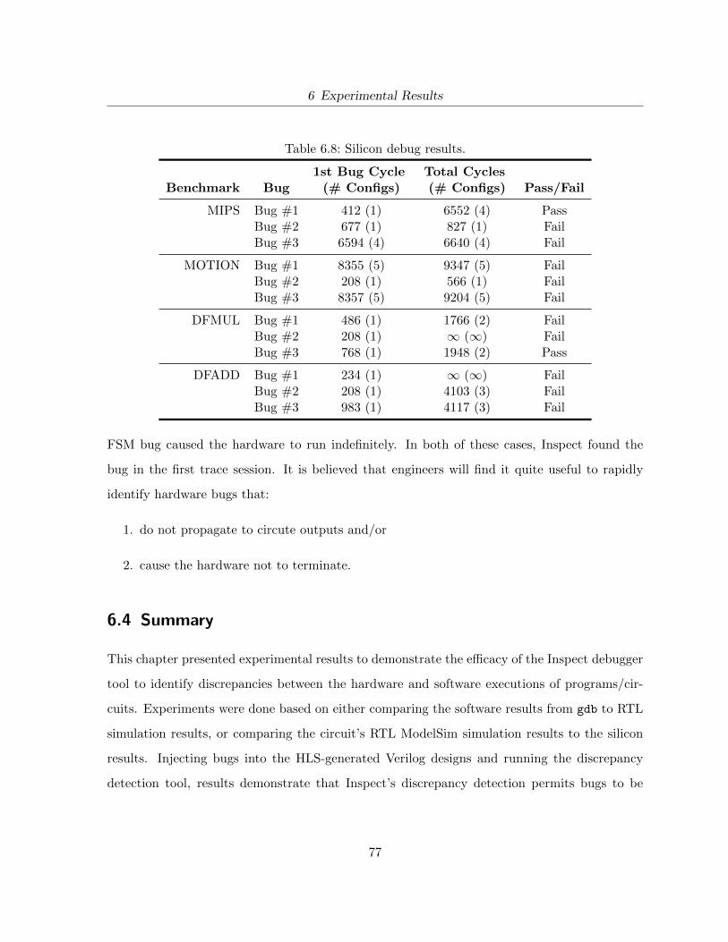
6 Experimental Results
Table 6.8: Silicon debug results.
1st Bug Cycle Total CyclesBenchmark Bug (# Configs) (# Configs) Pass/Fail
MIPS Bug #1 412 (1) 6552 (4) PassBug #2 677 (1) 827 (1) FailBug #3 6594 (4) 6640 (4) Fail
MOTION Bug #1 8355 (5) 9347 (5) FailBug #2 208 (1) 566 (1) FailBug #3 8357 (5) 9204 (5) Fail
DFMUL Bug #1 486 (1) 1766 (2) FailBug #2 208 (1) ∞ (∞) FailBug #3 768 (1) 1948 (2) Pass
DFADD Bug #1 234 (1) ∞ (∞) FailBug #2 208 (1) 4103 (3) FailBug #3 983 (1) 4117 (3) Fail
FSM bug caused the hardware to run indefinitely. In both of these cases, Inspect found the
bug in the first trace session. It is believed that engineers will find it quite useful to rapidly
identify hardware bugs that:
1. do not propagate to circute outputs and/or
2. cause the hardware not to terminate.
6.4 Summary
This chapter presented experimental results to demonstrate the efficacy of the Inspect debugger
tool to identify discrepancies between the hardware and software executions of programs/cir-
cuits. Experiments were done based on either comparing the software results from gdb to RTL
simulation results, or comparing the circuit’s RTL ModelSim simulation results to the silicon
results. Injecting bugs into the HLS-generated Verilog designs and running the discrepancy
detection tool, results demonstrate that Inspect’s discrepancy detection permits bugs to be
77
6 Experimental Results
discovered in significantly fewer cycles than if they must propagate to circuit outputs. It was
also shown that Inspect is capable of detecting bugs that affect internal signals and may not
change the circuit outputs for the given test vectors, and also bugs that cause the hardware to
continue to execute indefinitely.
78

7 Conclusion and Future Work
7.1 Conclusion
Long-term vision for high-level synthesis is to make the speed and energy benefits of hardware
accessible to software engineers, and significant progress has been made in recent years in
the quality of circuits produced by HLS. What is needed to realize that vision, however, are
debugging tools that offer a software engineer’s perspective into the auto-generated hardware.
This is accomplished through the creation of the Inspect debugger that provides a software
perspective for debugging LegUp-generated hardware designs.
The Inspect framework list of features are:
• C source-level debugging for HLS-generated hardware, that gives the user familiar step,
run and break features, and the ability to watch variables, where the values are drawn
from the hardware: either RTL simulation or execution in silicon. For the RTL simulation,
Inspect connects to and uses the ModelSim logic simulator and for the silicon execution,
it connects with Altera’s Quartus CAD tools and the SignalTap II Logic Analyzer.
• Ability to view the relations between three levels of program/circuit abstraction: C, LLVM
IR, and Verilog. With Inspect, stepping through the C statements highlights the relevant
executing IR instructions, and selecting any IR instruction shows the relevant parts of
the Verilog code to the user.
• Beyond the traditional gdb-like functionality, Inspect provides automated discrepancy
detection between hardware and software for quick pinpointing of HW/SW differences.
79
7 Conclusion and Future Work
7.2 Future Work
Since debugging for HLS is a relatively new area of research, there are many topics that can be
explored in future research. Some of them are discussed below:
7.2.1 Debugging Optimized Code
Presently, Inspect works best with an unoptimized version of the program. One future research
direction is to improve the correlation between software and hardware, when the hardware is
generated with compiler optimizations turned on. This could be challenging, because:
• Currently, Inspect framework tracks the load and store instructions to find when the
memories/variables are changed. In presence of optimizations, many load and store
instructions would be removed by the LLVM compiler, making it impossible for Inspect
framework to track value changes for all source-level variables.
• Instructions ordering may change when the optimizations are turned on, that can cause
the IR and C codes to be very different in structure. By having a different instruction
ordering in the IR level, the active statement from the source-level perspective, may jump
around without any meaningful pattern to the user, unless the debugging framework
handles the reordering.
While Inspect presents the best debugging experience with the optimizations turned off, it
is capable of debugging optimized code as well with some limitations such as jumping around
statements and not providing values for the variables that are removed due to optimizations. It
is worth mentioning that most debuggers (including gdb) also have limitations when working
with optimized binaries. Currently, LegUp HLS tool works with the LLVM version 2.9 and
we expect to have more accurate debugging information during the optimized code debug, by
using the most recent LLVM framework.
80
7 Conclusion and Future Work
7.2.2 LLDB support
Presently, Inspect uses the combination of clang and gdb in order to compile and debug the
program in software mode during the discrepancy detection. It is observed that gdb function-
ality is not guaranteed when using the clang binaries. In order to provide full support for
debugging clang binaries, replacing the gdb debugger with the LLVM debugging framework –
LLDB [22] is required. However, LLDB is only supported in the most recent versions of the
LLVM framework which are not still supported by the LegUp HLS tool.
7.2.3 Hybrid Flow Debugging
The current work focused on debugging designs that are entirely compiled to Verilog. A direc-
tion for future work is enabling the debug for hybrid systems, in which the program is compiled
to hybrid hardware/software system comprising a processor along with one or more accelerators.
7.2.4 Supporting LegUp-Specific Optimizations
There are some LegUp optimization directives that are not supported in the current version
of the Inspect debugger. These include loop-pipelining and pthread-openMP features, where
parallel software threads are automatically translated into parallel hardware accelerators [10].
To support pthread-openMP feature in the Inspect debugger, one idea is to equip Inspect
with similar features to GPU debuggers to identify different threads in the program/design and
provide visibility among all running threads. The idea is presented in [19] which automatically
instruments recording code to the input GPU stream program. The instrumented code keeps
all information about GPU memory operations. There is also a dataflow visualizer allowing the
user to examine the memory operation values in all streams. Using the recorded dataflow, the
user can discover errors by tracing through relevant threads and streams. We also would like
to investigate using partial orders techniques for parallel debugging [15] to be able to have the
pthread-openMP optimization enabled while performing discrepancy detection algorithm.
81

7 Conclusion and Future Work
7.2.5 Debugging Multiple Clock Domain Designs
Another direction for future research is debugging designs with multiple clock domains. There
are several issues to address while debugging these designs such as updating/representing sig-
nals/variables values with regards to their own clock domain and being able to proceed the
design and capture signal values in multiple clock domains simultaneously. For the silicon-
debug, we will investigate creating different SignalTap configuration files for each clock domain
and capture each domain’s data separately, while finally organizing them all in one location.
7.2.6 Bug Fixing
We recognize that in Inspect’s current form, it may be difficult for a software engineer to fix a
bug detected by one of the discrepancy detection flows – such corrections may require hardware
skills. The software engineer may, for example, consider re-writing the C in a different style in
the hope that the resulting HLS-generated hardware would be changed. A direction for future
work is a “wizard-like” functionality within the debugger to suggest code fixes to the user for
each bug detected.
82

A Inspect Debug Database SQL Script
Below is the SQL script that is used by Inspect to create the debug database.
SET @OLD UNIQUE CHECKS=@@UNIQUE CHECKS, UNIQUE CHECKS=0;
SET @OLD FOREIGN KEY CHECKS=@@FOREIGN KEY CHECKS, FOREIGN KEY CHECKS=0;
SET @OLD SQL MODE=@@SQL MODE, SQL MODE=’TRADITIONAL,ALLOW INVALID DATES ’ ;
CREATE SCHEMA IF NOT EXISTS ‘ in spect db ‘ DEFAULT CHARACTER SET l a t i n 1 ;
USE ‘ inspect db ‘ ;
−− −−−−−−−−−−−−−−−−−−−−−−−−−−−−−−−−−−−−−−−−−−−−−−−−−−−−−−− Table ‘ i n s p e c t d b ‘ . ‘ Function ‘
−− −−−−−−−−−−−−−−−−−−−−−−−−−−−−−−−−−−−−−−−−−−−−−−−−−−−−−CREATE TABLE IF NOT EXISTS ‘ in spect db ‘ . ‘ Function ‘ (
‘ id ‘ INT(11) NOT NULL AUTO INCREMENT ,
‘name ‘ VARCHAR(100) NULL DEFAULT NULL ,
‘ startLineNumber ‘ INT(11) NULL ,
PRIMARY KEY ( ‘ id ‘ ) )
ENGINE = InnoDB
DEFAULT CHARACTER SET = l a t i n 1
COLLATE = l a t i n 1 s w e d i s h c i ;
−− −−−−−−−−−−−−−−−−−−−−−−−−−−−−−−−−−−−−−−−−−−−−−−−−−−−−−−− Table ‘ i n s p e c t d b ‘ . ‘ HLStatement ‘
−− −−−−−−−−−−−−−−−−−−−−−−−−−−−−−−−−−−−−−−−−−−−−−−−−−−−−−CREATE TABLE IF NOT EXISTS ‘ in spect db ‘ . ‘ HLStatement ‘ (
‘ id ‘ INT(11) NOT NULL AUTO INCREMENT ,
‘ l ine number ‘ INT(11) NULL DEFAULT NULL ,
83

A Inspect Debug Database SQL Script
‘ column number ‘ INT(11) NULL ,
‘ f i l e name ‘ VARCHAR(100) NULL DEFAULT NULL ,
PRIMARY KEY ( ‘ id ‘ ) )
ENGINE = InnoDB
DEFAULT CHARACTER SET = l a t i n 1 ;
−− −−−−−−−−−−−−−−−−−−−−−−−−−−−−−−−−−−−−−−−−−−−−−−−−−−−−−−− Table ‘ i n s p e c t d b ‘ . ‘ IRInstr ‘
−− −−−−−−−−−−−−−−−−−−−−−−−−−−−−−−−−−−−−−−−−−−−−−−−−−−−−−CREATE TABLE IF NOT EXISTS ‘ in spect db ‘ . ‘ IRInstr ‘ (
‘ id ‘ INT NOT NULL AUTO INCREMENT ,
‘ number in funct ion ‘ INT(11) NOT NULL ,
‘ f u n c t i o n i d ‘ INT(11) NOT NULL ,
‘ HLStatement id ‘ INT(11) NULL ,
‘dump‘ VARCHAR(2000) NULL ,
INDEX ‘ f k IRIn s t r HLIns t r i dx ‘ ( ‘ HLStatement id ‘ ASC) ,
INDEX ‘ f k IRIns t r Func t i on1 idx ‘ ( ‘ f u n c t i o n i d ‘ ASC) ,
PRIMARY KEY ( ‘ id ‘ ) ,
CONSTRAINT ‘ f k IRIns t r HLIns t r ‘
FOREIGN KEY ( ‘ HLStatement id ‘ )
REFERENCES ‘ inspect db ‘ . ‘ HLStatement ‘ ( ‘ id ‘ )
ON DELETE CASCADE
ON UPDATE CASCADE,
CONSTRAINT ‘ f k IRIns t r Funct ion1 ‘
FOREIGN KEY ( ‘ f u n c t i o n i d ‘ )
REFERENCES ‘ inspect db ‘ . ‘ Function ‘ ( ‘ id ‘ )
ON DELETE CASCADE
ON UPDATE CASCADE)
ENGINE = InnoDB
DEFAULT CHARACTER SET = l a t i n 1 ;
−− −−−−−−−−−−−−−−−−−−−−−−−−−−−−−−−−−−−−−−−−−−−−−−−−−−−−−
84
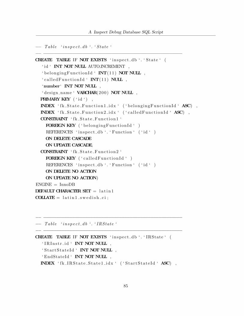
A Inspect Debug Database SQL Script
−− Table ‘ i n s p e c t d b ‘ . ‘ State ‘
−− −−−−−−−−−−−−−−−−−−−−−−−−−−−−−−−−−−−−−−−−−−−−−−−−−−−−−CREATE TABLE IF NOT EXISTS ‘ in spect db ‘ . ‘ State ‘ (
‘ id ‘ INT NOT NULL AUTO INCREMENT ,
‘ be longingFunct ionId ‘ INT(11) NOT NULL ,
‘ ca l l edFunct ionId ‘ INT(11) NULL ,
‘number ‘ INT NOT NULL ,
‘ design name ‘ VARCHAR(200) NOT NULL ,
PRIMARY KEY ( ‘ id ‘ ) ,
INDEX ‘ f k S ta t e Func t i on1 idx ‘ ( ‘ be longingFunct ionId ‘ ASC) ,
INDEX ‘ f k S ta t e Func t i on2 idx ‘ ( ‘ ca l l edFunct ionId ‘ ASC) ,
CONSTRAINT ‘ f k State Funct ion1 ‘
FOREIGN KEY ( ‘ be longingFunct ionId ‘ )
REFERENCES ‘ inspect db ‘ . ‘ Function ‘ ( ‘ id ‘ )
ON DELETE CASCADE
ON UPDATE CASCADE,
CONSTRAINT ‘ f k State Funct ion2 ‘
FOREIGN KEY ( ‘ ca l l edFunct ionId ‘ )
REFERENCES ‘ inspect db ‘ . ‘ Function ‘ ( ‘ id ‘ )
ON DELETE NO ACTION
ON UPDATE NO ACTION)
ENGINE = InnoDB
DEFAULT CHARACTER SET = l a t i n 1
COLLATE = l a t i n 1 s w e d i s h c i ;
−− −−−−−−−−−−−−−−−−−−−−−−−−−−−−−−−−−−−−−−−−−−−−−−−−−−−−−−− Table ‘ i n s p e c t d b ‘ . ‘ IRState ‘
−− −−−−−−−−−−−−−−−−−−−−−−−−−−−−−−−−−−−−−−−−−−−−−−−−−−−−−CREATE TABLE IF NOT EXISTS ‘ in spect db ‘ . ‘ IRState ‘ (
‘ IRIns t r i d ‘ INT NOT NULL ,
‘ S ta r tState Id ‘ INT NOT NULL ,
‘ EndStateId ‘ INT NOT NULL ,
INDEX ‘ f k IRSta t e S ta t e1 idx ‘ ( ‘ S tar tState Id ‘ ASC) ,
85
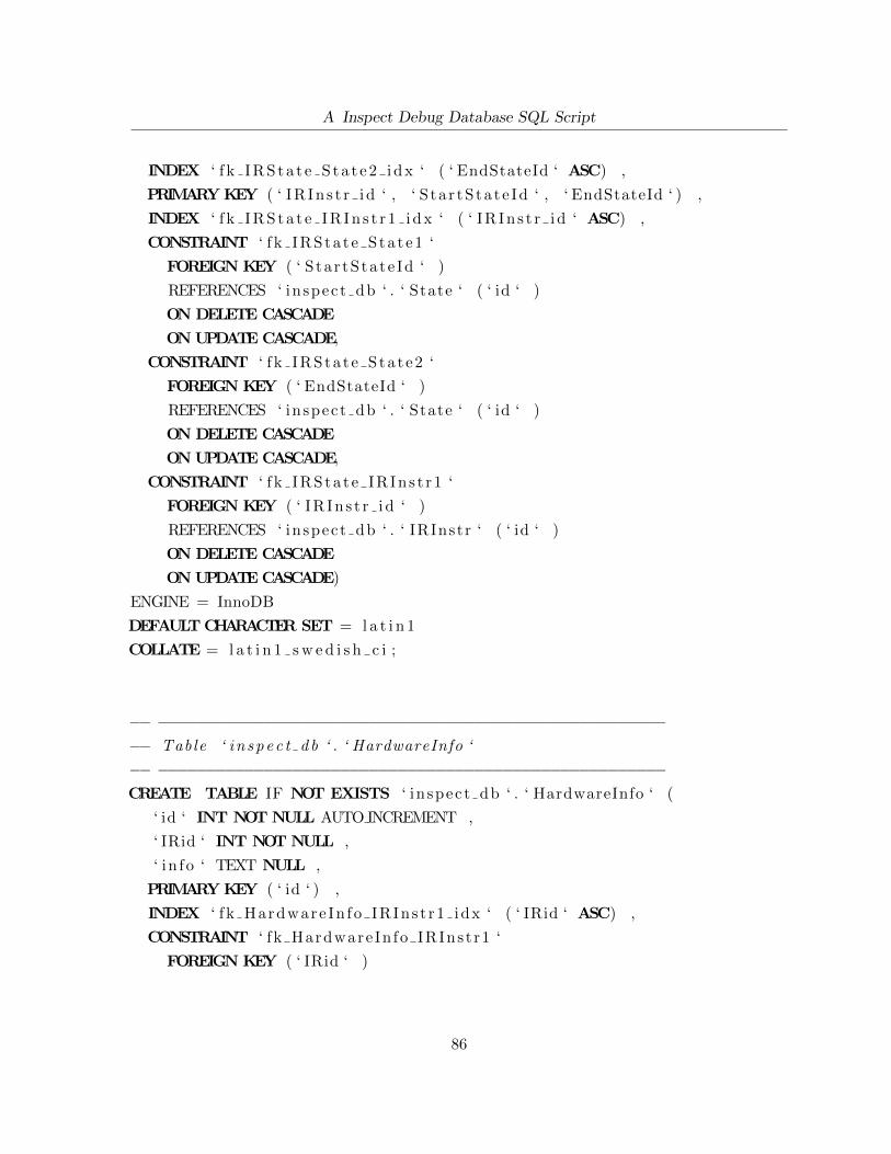
A Inspect Debug Database SQL Script
INDEX ‘ f k IRSta t e S ta t e2 idx ‘ ( ‘ EndStateId ‘ ASC) ,
PRIMARY KEY ( ‘ IRIn s t r i d ‘ , ‘ S ta r tState Id ‘ , ‘ EndStateId ‘ ) ,
INDEX ‘ f k I RSt a t e IR In s t r 1 id x ‘ ( ‘ IRIns t r i d ‘ ASC) ,
CONSTRAINT ‘ f k IRState Sta te1 ‘
FOREIGN KEY ( ‘ S ta r tState Id ‘ )
REFERENCES ‘ inspect db ‘ . ‘ State ‘ ( ‘ id ‘ )
ON DELETE CASCADE
ON UPDATE CASCADE,
CONSTRAINT ‘ f k IRState Sta te2 ‘
FOREIGN KEY ( ‘ EndStateId ‘ )
REFERENCES ‘ inspect db ‘ . ‘ State ‘ ( ‘ id ‘ )
ON DELETE CASCADE
ON UPDATE CASCADE,
CONSTRAINT ‘ f k IRSta te IRIns t r1 ‘
FOREIGN KEY ( ‘ IRIn s t r i d ‘ )
REFERENCES ‘ inspect db ‘ . ‘ IRInstr ‘ ( ‘ id ‘ )
ON DELETE CASCADE
ON UPDATE CASCADE)
ENGINE = InnoDB
DEFAULT CHARACTER SET = l a t i n 1
COLLATE = l a t i n 1 s w e d i s h c i ;
−− −−−−−−−−−−−−−−−−−−−−−−−−−−−−−−−−−−−−−−−−−−−−−−−−−−−−−−− Table ‘ i n s p e c t d b ‘ . ‘ HardwareInfo ‘
−− −−−−−−−−−−−−−−−−−−−−−−−−−−−−−−−−−−−−−−−−−−−−−−−−−−−−−CREATE TABLE IF NOT EXISTS ‘ in spect db ‘ . ‘ HardwareInfo ‘ (
‘ id ‘ INT NOT NULL AUTO INCREMENT ,
‘ IRid ‘ INT NOT NULL ,
‘ i n fo ‘ TEXT NULL ,
PRIMARY KEY ( ‘ id ‘ ) ,
INDEX ‘ f k Hardware In fo IRIns t r1 idx ‘ ( ‘ IRid ‘ ASC) ,
CONSTRAINT ‘ fk HardwareIn fo IRInst r1 ‘
FOREIGN KEY ( ‘ IRid ‘ )
86
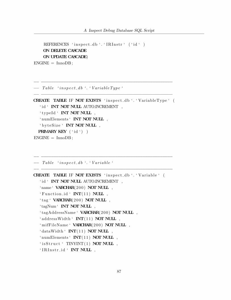
A Inspect Debug Database SQL Script
REFERENCES ‘ inspect db ‘ . ‘ IRInstr ‘ ( ‘ id ‘ )
ON DELETE CASCADE
ON UPDATE CASCADE)
ENGINE = InnoDB ;
−− −−−−−−−−−−−−−−−−−−−−−−−−−−−−−−−−−−−−−−−−−−−−−−−−−−−−−−− Table ‘ i n s p e c t d b ‘ . ‘ VariableType ‘
−− −−−−−−−−−−−−−−−−−−−−−−−−−−−−−−−−−−−−−−−−−−−−−−−−−−−−−CREATE TABLE IF NOT EXISTS ‘ in spect db ‘ . ‘ VariableType ‘ (
‘ id ‘ INT NOT NULL AUTO INCREMENT ,
‘ typeId ‘ INT NOT NULL ,
‘ numElements ‘ INT NOT NULL ,
‘ byteSize ‘ INT NOT NULL ,
PRIMARY KEY ( ‘ id ‘ ) )
ENGINE = InnoDB ;
−− −−−−−−−−−−−−−−−−−−−−−−−−−−−−−−−−−−−−−−−−−−−−−−−−−−−−−−− Table ‘ i n s p e c t d b ‘ . ‘ Variab le ‘
−− −−−−−−−−−−−−−−−−−−−−−−−−−−−−−−−−−−−−−−−−−−−−−−−−−−−−−CREATE TABLE IF NOT EXISTS ‘ in spect db ‘ . ‘ Var iable ‘ (
‘ id ‘ INT NOT NULL AUTO INCREMENT ,
‘name ‘ VARCHAR(200) NOT NULL ,
‘ Funct ion id ‘ INT(11) NULL ,
‘ tag ‘ VARCHAR(200) NOT NULL ,
‘ tagNum ‘ INT NOT NULL ,
‘ tagAddressName ‘ VARCHAR(200) NOT NULL ,
‘ addressWidth ‘ INT(11) NOT NULL ,
‘ mifFileName ‘ VARCHAR(200) NOT NULL ,
‘ dataWidth ‘ INT(11) NOT NULL ,
‘ numElements ‘ INT(11) NOT NULL ,
‘ i s S t r u c t ‘ TINYINT(1) NOT NULL ,
‘ IR Ins t r i d ‘ INT NULL ,
87

A Inspect Debug Database SQL Script
‘ type ‘ VARCHAR(45) NOT NULL ,
‘ debugTypeId ‘ INT NOT NULL ,
PRIMARY KEY ( ‘ id ‘ ) ,
INDEX ‘ f k Var i ab l e Func t i on1 idx ‘ ( ‘ Funct ion id ‘ ASC) ,
INDEX ‘ f k V a r i a b l e I R I n s t r 1 i d x ‘ ( ‘ IRIn s t r i d ‘ ASC) ,
INDEX ‘ f k Var iab l e Var iab l eType1 idx ‘ ( ‘ debugTypeId ‘ ASC) ,
CONSTRAINT ‘ f k Var iab l e Funct ion1 ‘
FOREIGN KEY ( ‘ Funct ion id ‘ )
REFERENCES ‘ inspect db ‘ . ‘ Function ‘ ( ‘ id ‘ )
ON DELETE CASCADE
ON UPDATE CASCADE,
CONSTRAINT ‘ f k V a r i a b l e I R I n s t r 1 ‘
FOREIGN KEY ( ‘ IRIn s t r i d ‘ )
REFERENCES ‘ inspect db ‘ . ‘ IRInstr ‘ ( ‘ id ‘ )
ON DELETE CASCADE
ON UPDATE CASCADE,
CONSTRAINT ‘ fk Var iab le Var iab leType1 ‘
FOREIGN KEY ( ‘ debugTypeId ‘ )
REFERENCES ‘ inspect db ‘ . ‘ VariableType ‘ ( ‘ id ‘ )
ON DELETE CASCADE
ON UPDATE CASCADE)
ENGINE = InnoDB ;
−− −−−−−−−−−−−−−−−−−−−−−−−−−−−−−−−−−−−−−−−−−−−−−−−−−−−−−−− Table ‘ i n s p e c t d b ‘ . ‘ HWSignal ‘
−− −−−−−−−−−−−−−−−−−−−−−−−−−−−−−−−−−−−−−−−−−−−−−−−−−−−−−CREATE TABLE IF NOT EXISTS ‘ in spect db ‘ . ‘ HWSignal ‘ (
‘ id ‘ INT NOT NULL AUTO INCREMENT ,
‘name ‘ VARCHAR(100) NULL ,
‘ width ‘ INT(11) NULL ,
‘ f u n c t i o n i d ‘ INT(11) NOT NULL ,
‘ i sConst ‘ TINYINT(1) NOT NULL ,
‘ Var i ab l e id ‘ INT NULL ,
88

A Inspect Debug Database SQL Script
PRIMARY KEY ( ‘ id ‘ ) ,
INDEX ‘ f k S i gna l Func t i on1 idx ‘ ( ‘ f u n c t i o n i d ‘ ASC) ,
INDEX ‘ fk HWSignal Var iable1 idx ‘ ( ‘ Var i ab l e id ‘ ASC) ,
CONSTRAINT ‘ f k S igna l Funct i on1 ‘
FOREIGN KEY ( ‘ f u n c t i o n i d ‘ )
REFERENCES ‘ inspect db ‘ . ‘ Function ‘ ( ‘ id ‘ )
ON DELETE CASCADE
ON UPDATE CASCADE,
CONSTRAINT ‘ fk HWSignal Variable1 ‘
FOREIGN KEY ( ‘ Var i ab l e id ‘ )
REFERENCES ‘ inspect db ‘ . ‘ Var iable ‘ ( ‘ id ‘ )
ON DELETE CASCADE
ON UPDATE CASCADE)
ENGINE = InnoDB ;
−− −−−−−−−−−−−−−−−−−−−−−−−−−−−−−−−−−−−−−−−−−−−−−−−−−−−−−−− Table ‘ i n s p e c t d b ‘ . ‘ I n s t r u c t i o n S i g n a l ‘
−− −−−−−−−−−−−−−−−−−−−−−−−−−−−−−−−−−−−−−−−−−−−−−−−−−−−−−CREATE TABLE IF NOT EXISTS ‘ in spect db ‘ . ‘ I n s t r u c t i o n S i g n a l ‘ (
‘ HWSignal id ‘ INT NOT NULL ,
‘ IR Ins t r i d ‘ INT NOT NULL ,
INDEX ‘ f k In s t ruc t i onS igna l HWSigna l1 idx ‘ ( ‘ HWSignal id ‘ ASC) ,
INDEX ‘ f k I n s t r u c t i o n S i g n a l I R I n s t r 1 i d x ‘ ( ‘ IRIn s t r i d ‘ ASC) ,
CONSTRAINT ‘ f k Ins t ruct ionS igna l HWSigna l1 ‘
FOREIGN KEY ( ‘ HWSignal id ‘ )
REFERENCES ‘ inspect db ‘ . ‘ HWSignal ‘ ( ‘ id ‘ )
ON DELETE NO ACTION
ON UPDATE NO ACTION,
CONSTRAINT ‘ f k I n s t r u c t i o n S i g n a l I R I n s t r 1 ‘
FOREIGN KEY ( ‘ IRIn s t r i d ‘ )
REFERENCES ‘ inspect db ‘ . ‘ IRInstr ‘ ( ‘ id ‘ )
ON DELETE NO ACTION
ON UPDATE NO ACTION)
89
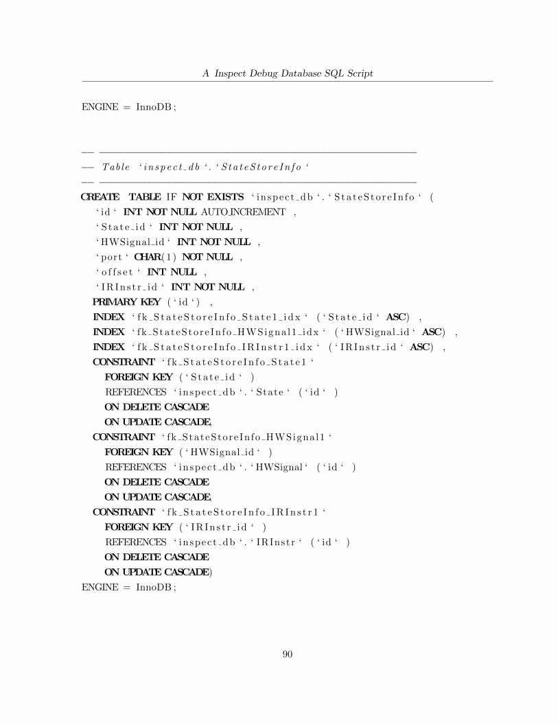
A Inspect Debug Database SQL Script
ENGINE = InnoDB ;
−− −−−−−−−−−−−−−−−−−−−−−−−−−−−−−−−−−−−−−−−−−−−−−−−−−−−−−−− Table ‘ i n s p e c t d b ‘ . ‘ S t a t e S t o r e I n f o ‘
−− −−−−−−−−−−−−−−−−−−−−−−−−−−−−−−−−−−−−−−−−−−−−−−−−−−−−−CREATE TABLE IF NOT EXISTS ‘ in spect db ‘ . ‘ S ta t eS to r e In fo ‘ (
‘ id ‘ INT NOT NULL AUTO INCREMENT ,
‘ S ta t e id ‘ INT NOT NULL ,
‘ HWSignal id ‘ INT NOT NULL ,
‘ port ‘ CHAR(1 ) NOT NULL ,
‘ o f f s e t ‘ INT NULL ,
‘ IR Ins t r i d ‘ INT NOT NULL ,
PRIMARY KEY ( ‘ id ‘ ) ,
INDEX ‘ f k S t a t e S t o r e I n f o S t a t e 1 i d x ‘ ( ‘ S ta t e id ‘ ASC) ,
INDEX ‘ f k StateStore In fo HWSigna l1 idx ‘ ( ‘ HWSignal id ‘ ASC) ,
INDEX ‘ f k S t a t e S t o r e I n f o I R I n s t r 1 i d x ‘ ( ‘ IRIn s t r i d ‘ ASC) ,
CONSTRAINT ‘ f k S t a t e S t o r e I n f o S t a t e 1 ‘
FOREIGN KEY ( ‘ S ta t e id ‘ )
REFERENCES ‘ inspect db ‘ . ‘ State ‘ ( ‘ id ‘ )
ON DELETE CASCADE
ON UPDATE CASCADE,
CONSTRAINT ‘ fk StateStoreIn fo HWSignal1 ‘
FOREIGN KEY ( ‘ HWSignal id ‘ )
REFERENCES ‘ inspect db ‘ . ‘ HWSignal ‘ ( ‘ id ‘ )
ON DELETE CASCADE
ON UPDATE CASCADE,
CONSTRAINT ‘ f k S t a t e S t o r e I n f o I R I n s t r 1 ‘
FOREIGN KEY ( ‘ IRIn s t r i d ‘ )
REFERENCES ‘ inspect db ‘ . ‘ IRInstr ‘ ( ‘ id ‘ )
ON DELETE CASCADE
ON UPDATE CASCADE)
ENGINE = InnoDB ;
90
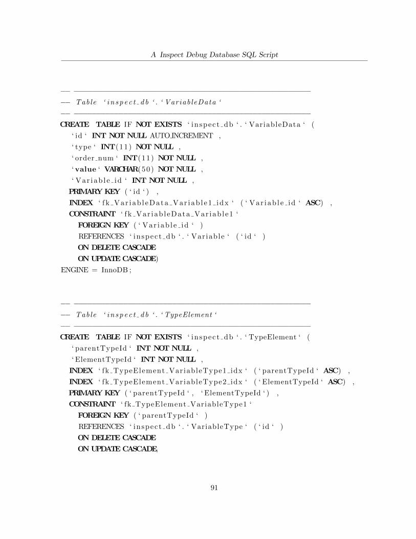
A Inspect Debug Database SQL Script
−− −−−−−−−−−−−−−−−−−−−−−−−−−−−−−−−−−−−−−−−−−−−−−−−−−−−−−−− Table ‘ i n s p e c t d b ‘ . ‘ VariableData ‘
−− −−−−−−−−−−−−−−−−−−−−−−−−−−−−−−−−−−−−−−−−−−−−−−−−−−−−−CREATE TABLE IF NOT EXISTS ‘ in spect db ‘ . ‘ VariableData ‘ (
‘ id ‘ INT NOT NULL AUTO INCREMENT ,
‘ type ‘ INT(11) NOT NULL ,
‘ order num ‘ INT(11) NOT NULL ,
‘ value ‘ VARCHAR(50) NOT NULL ,
‘ Var i ab l e id ‘ INT NOT NULL ,
PRIMARY KEY ( ‘ id ‘ ) ,
INDEX ‘ f k Var i ab l eData Var iab l e1 idx ‘ ( ‘ Var i ab l e id ‘ ASC) ,
CONSTRAINT ‘ f k Var iab l eData Var iab l e1 ‘
FOREIGN KEY ( ‘ Var i ab l e id ‘ )
REFERENCES ‘ inspect db ‘ . ‘ Var iable ‘ ( ‘ id ‘ )
ON DELETE CASCADE
ON UPDATE CASCADE)
ENGINE = InnoDB ;
−− −−−−−−−−−−−−−−−−−−−−−−−−−−−−−−−−−−−−−−−−−−−−−−−−−−−−−−− Table ‘ i n s p e c t d b ‘ . ‘ TypeElement ‘
−− −−−−−−−−−−−−−−−−−−−−−−−−−−−−−−−−−−−−−−−−−−−−−−−−−−−−−CREATE TABLE IF NOT EXISTS ‘ in spect db ‘ . ‘ TypeElement ‘ (
‘ parentTypeId ‘ INT NOT NULL ,
‘ ElementTypeId ‘ INT NOT NULL ,
INDEX ‘ fk TypeElement VariableType1 idx ‘ ( ‘ parentTypeId ‘ ASC) ,
INDEX ‘ fk TypeElement VariableType2 idx ‘ ( ‘ ElementTypeId ‘ ASC) ,
PRIMARY KEY ( ‘ parentTypeId ‘ , ‘ ElementTypeId ‘ ) ,
CONSTRAINT ‘ fk TypeElement VariableType1 ‘
FOREIGN KEY ( ‘ parentTypeId ‘ )
REFERENCES ‘ inspect db ‘ . ‘ VariableType ‘ ( ‘ id ‘ )
ON DELETE CASCADE
ON UPDATE CASCADE,
91

A Inspect Debug Database SQL Script
CONSTRAINT ‘ fk TypeElement VariableType2 ‘
FOREIGN KEY ( ‘ ElementTypeId ‘ )
REFERENCES ‘ inspect db ‘ . ‘ VariableType ‘ ( ‘ id ‘ )
ON DELETE CASCADE
ON UPDATE CASCADE)
ENGINE = InnoDB ;
USE ‘ inspect db ‘ ;
SET SQL MODE=@OLD SQL MODE;
SET FOREIGN KEY CHECKS=@OLD FOREIGN KEY CHECKS;
SET UNIQUE CHECKS=@OLD UNIQUE CHECKS;
92

B LLVM Framework Instructions Reference
Below is the list of most important LLVM instructions obtained from LLVM language reference
manual [23]. For the complete list, interested readers are referred to [23].
B.1 Terminator Instructions
B.1.1 ‘ret’ Instruction
The ‘ret’ instruction is used to return control flow (and optionally a value) from a function
back to the caller. There are two forms of the ‘ret’ instruction: one that returns a value
and then causes control flow, and one that just causes control flow to occur. When the ‘ret’
instruction is executed, control flow returns back to the calling functions context. If the caller
is a “call” instruction, execution continues at the instruction after the call. If the caller was an
invoke instruction, execution continues at the beginning of the normal destination block. If the
instruction returns a value, that value shall set the call or invoke instructions return value.
B.1.2 ‘br’ Instruction
The ‘br’ instruction is used to cause control flow to transfer to a different basic block in the
current function. There are two forms of this instruction, corresponding to a conditional branch
and an unconditional branch. Upon execution of a conditional ‘br’ instruction, the condition is
evaluated. If the value is true, control flows to the first label, otherwise to the other one.
93

B LLVM Framework Instructions Reference
B.2 Binary Instructions
B.2.1 ‘add’ Instruction
The ‘add’ instruction returns the sum of its two operands. The value produced is the integer
sum of the two operands. If the sum has unsigned overflow, the result returned is the mathe-
matical result modulo 2n, where n is the bit width of the result. Because LLVM integers use a
twos complement representation, this instruction is appropriate for both signed and unsigned
integers.
B.2.2 ‘sub’ Instruction
The ‘sub’ instruction returns the difference of its two operands. Note that the ‘sub’ instruction
is used to represent the ‘neg’ instruction present in most other intermediate representations.
The value produced is the integer difference of the two operands. If the difference has unsigned
overflow, the result returned is the mathematical result modulo 2n, where n is the bit width of
the result. Because LLVM integers use a twos complement representation, this instruction is
appropriate for both signed and unsigned integers.
B.2.3 ‘mul’ Instruction
The ‘mul’ instruction returns the product of its two operands. The value produced is the integer
product of the two operands. If the result of the multiplication has unsigned overflow, the result
returned is the mathematical result modulo 2n, where n is the bit width of the result. Because
LLVM integers use a two’s complement representation, and the result is the same width as the
operands, this instruction returns the correct result for both signed and unsigned integers.
B.2.4 ‘udiv’ Instruction
The ‘udiv’ instruction returns the quotient of its two operands. The value produced is the
unsigned integer quotient of the two operands. Since unsigned integer division and signed integer
94
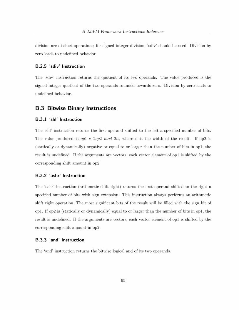
B LLVM Framework Instructions Reference
division are distinct operations; for signed integer division, ‘sdiv’ should be used. Division by
zero leads to undefined behavior.
B.2.5 ’sdiv’ Instruction
The ‘sdiv’ instruction returns the quotient of its two operands. The value produced is the
signed integer quotient of the two operands rounded towards zero. Division by zero leads to
undefined behavior.
B.3 Bitwise Binary Instructions
B.3.1 ‘shl’ Instruction
The ‘shl’ instruction returns the first operand shifted to the left a specified number of bits.
The value produced is op1 ∗ 2op2 mod 2n, where n is the width of the result. If op2 is
(statically or dynamically) negative or equal to or larger than the number of bits in op1, the
result is undefined. If the arguments are vectors, each vector element of op1 is shifted by the
corresponding shift amount in op2.
B.3.2 ‘ashr’ Instruction
The ‘ashr’ instruction (arithmetic shift right) returns the first operand shifted to the right a
specified number of bits with sign extension. This instruction always performs an arithmetic
shift right operation, The most significant bits of the result will be filled with the sign bit of
op1. If op2 is (statically or dynamically) equal to or larger than the number of bits in op1, the
result is undefined. If the arguments are vectors, each vector element of op1 is shifted by the
corresponding shift amount in op2.
B.3.3 ‘and’ Instruction
The ‘and’ instruction returns the bitwise logical and of its two operands.
95

B LLVM Framework Instructions Reference
B.3.4 ‘or’ Instruction
The ‘or’ instruction returns the bitwise logical inclusive or of its two operands.
B.4 Memory Accessing and Addressing Instructions
B.4.1 ‘alloca’ Instruction
The ‘alloca’ instruction allocates memory on the stack frame of the currently executing function,
to be automatically released when this function returns to its caller. The object is always
allocated in the generic address space (address space zero). Memory is allocated; a pointer
is returned. The operation is undefined if there is insufficient stack space for the allocation.
‘alloca’d memory is automatically released when the function returns. The ‘alloca’ instruction
is commonly used to represent automatic variables that must have an address available. When
the function returns (either with the ret or resume instructions), the memory is reclaimed.
Allocating zero bytes is legal, but the result is undefined. The order in which memory is
allocated (ie., which way the stack grows) is not specified.
B.4.2 ‘load’ Instruction
The ‘load’ instruction is used to read from memory. The location of memory pointed to is
loaded. If the value being loaded is of scalar type then the number of bytes read does not
exceed the minimum number of bytes needed to hold all bits of the type. For example, loading
an i24 reads at most three bytes.
B.4.3 ‘store’ Instruction
The ‘store’ instruction is used to write to memory. The contents of memory are updated to
contain < value > at the location specified by the < pointer > operand. If < value > is of
scalar type then the number of bytes written does not exceed the minimum number of bytes
needed to hold all bits of the type. For example, storing an i24 writes at most three bytes.
96
B LLVM Framework Instructions Reference
B.4.4 ‘getelementptr’ Instruction
The ‘getelementptr’ instruction is used to get the address of a subelement of an aggregate data
structure. It performs address calculation only and does not access memory.
The first argument is always a pointer or a vector of pointers, and forms the basis of the
calculation. The remaining arguments are indices that indicate which of the elements of the
aggregate object are indexed. The interpretation of each index is dependent on the type being
indexed into. The first index always indexes the pointer value given as the first argument,
the second index indexes a value of the type pointed to (not necessarily the value directly
pointed to, since the first index can be non-zero), etc. The first type indexed into must be a
pointer value, subsequent types can be arrays, vectors, and structs. Note that subsequent types
being indexed into can never be pointers, since that would require loading the pointer before
continuing calculation.
The type of each index argument depends on the type it is indexing into. When indexing
into a (optionally packed) structure, only i32 integer constants are allowed. When indexing
into an array, pointer or vector, integers of any width are allowed, and they are not required to
be constant. These integers are treated as signed values where relevant.
B.5 Conversion Instructions
B.5.1 ‘zext’ Instruction
The ‘zext’ instruction zero extends its operand to the destination type. The zext fills the high
order bits of the value with zero bits until it reaches the size of the destination type. When
zero extending from i1, the result will always be either 0 or 1.
B.5.2 ‘sext’ Instruction
The ‘sext’ sign extends value to the destination type. The ‘sext’ instruction performs a sign
extension by copying the sign bit (highest order bit) of the value until it reaches the bit size of
97

B LLVM Framework Instructions Reference
the destination type. When sign extending from i1, the extension always results in -1 or 0.
B.6 Other Instructions
B.6.1 ‘call’ Instruction
The ‘call’ instruction represents a simple function call. The call instruction is used to cause
control flow to transfer to a specified function, with its incoming arguments bound to the
specified values. Upon a ‘ret’ instruction in the called function, control flow continues with the
instruction after the function call, and the return value of the function is bound to the result
argument.
98
References
[1] C-based design: High-level synthesis with the Vivado HLS tool. Technical report, Xilinx
Incorporated, 2013.
[2] Certus ASIC prototyping debug solution. Technical report, Mentor Graphics Corp., 2014.
[3] Chipscope pro and the serial I/O toolkit. Technical report, Xilinx Incorporated, 2014.
[4] M. Aldham, J. Anderson, S. Brown, and A. Canis. Low-cost hardware profiling of run-time
and energy in FPGA embedded processors. In Application-Specific Systems, Architectures
and Processors (ASAP), 2011 IEEE International Conference on, pages 61–68. IEEE,
2011.
[5] Altera, Corp., San Jose, CA. Cyclone-IV Data Sheet, 2010.
[6] Altera, Corp., San Jose, CA. SignalTap II Logic Analyzer User Guide, 2013.
[7] A. Canis, J. H. Anderson, and S. D. Brown. Multi-pumping for resource reduction in
FPGA high-level synthesis. In Proceedings of the Conference on Design, Automation and
Test in Europe, pages 194–197. EDA Consortium, 2013.
[8] A. Canis, J. Choi, M. Aldham, V. Zhang, A. Kammoona, T. Czajkowski, S. D. Brown, and
J. H. Anderson. LegUp: An open source high-level synthesis tool for FPGA-based proces-
sor/accelerator systems. ACM Tranasactions on Embedded Computing Systems, 2013.
[9] D. Chen, J. Cong, Y. Fan, and Z. Zhang. High-level power estimation and low-power design
space exploration for FPGAs. In Asia and South Pacific Design Automation Conference,
pages 529–534, 2007.
99

B References
[10] J. Choi, S. Brown, and J. Anderson. From software threads to parallel hardware in high-
level synthesis for FPGAs. In Field-Programmable Technology (FPT), 2013 International
Conference on, pages 270–277. IEEE, 2013.
[11] J. Cong and Y. Zou. FPGA-based hardware acceleration of lithographic aerial image simu-
lation. ACM Transactions on Reconfigurable Technology and Systems (TRETS), 2(3):1–29,
2009.
[12] P. Coussy, G. Lhairech-Lebreton, D. Heller, and E. Martin. GAUT a free and open source
high-level synthesis tool. In IEEE DATE, 2010.
[13] P. Coussy and A. Morawiec. High-level synthesis. Springer, 2010.
[14] J. Curreri, G. Stitt, and A. D. George. High-level synthesis of in-circuit assertions for
verification, debugging, and timing analysis. International Journal of Reconfigurable Com-
puting, 2011.
[15] C. J. Fidge. Partial orders for parallel debugging. In ACM Sigplan Notices, volume 24,
pages 183–194. ACM, 1988.
[16] P. S. Graham. Logical hardware debuggers for FPGA-based systems. In Doctoral disser-
tation. Department of Electrical and Computer Engineering, Brigham Young University,
2001.
[17] Y. Hara, H. Tomiyama, S. Honda, and H. Takada. Proposal and quantitative analysis of
the CHStone benchmark program suite for practical C-based high-level synthesis. Journal
of Information Processing, 17:242–254, 2009.
[18] K. S. Hemmert, J. L. Tripp, B. L. Hutchings, and P. A. Jackson. Source level debugger
for the Sea Cucumber synthesizing compiler. IEEE FCCM, pages 228–237, 2003.
[19] Q. Hou, K. Zhou, and B. Guo. Debugging GPU stream programs through automatic
100

B References
dataflow recording and visualization. In ACM Transactions on Graphics (TOG), vol-
ume 28, page 153. ACM, 2009.
[20] http://calypto.com/en/products/catapult/overview. Calypto Catapult, 2013.
[21] http://libmigdb.sourceforge.net/. GDB/Machine Interface library, 2014.
[22] http://lldb.llvm.org/. The LLDB Debugger, 2014.
[23] http://llvm.org/docs/LangRef.html. LLVM Language Reference Manual, 2014.
[24] https://qt-project.org/. Qt Project Cross-platform Framework, 2014.
[25] http://www.altera.com/products/software/ opencl/opencl-index.html. OpenCL for Altera
FPGAs, 2013.
[26] http://www.gnu.org/software/gdb/. GDB The GNU Project Debugger, 2014.
[27] http://www.llvm.org. LLVM Compiler Infrastructure Project, 2014.
[28] http://www.monolithic3d.com/blog/. 28 nm - The Last Node of Moore’s Law, 2014.
[29] http://www.mysql.com. MySQL Open Source Database, 2014.
[30] http://www.xilinx.com/products/design tools/vivado/vivado-webpack.htm. Xilinx: Vi-
vado Design Suite, 2013.
[31] E. Hung and S. J. Wilton. Speculative debug insertion for FPGAs. Field Programmable
Logic and Applications (FPL), pages 524–531, 2011.
[32] B. Hutchings, P. Bellows, J. Hawkins, S. Hemmert, B. Nelson, and M. Rytting. A CAD
suite for high-performance FPGA design. In Field-Programmable Custom Computing Ma-
chines, 1999. FCCM’99. Proceedings. Seventh Annual IEEE Symposium on, pages 12–24.
IEEE, 1999.
101
B References
[33] Y. Liang, K. Rupnow, Y. Li, D. Min, M. N. Do, and D. Chen. High-level synthesis:
productivity, performance, and software constraints. Journal of Electrical and Computer
Engineering, 2012:1, 2012.
[34] J. Luu, I. Kuon, P. Jamieson, T. Campbell, A. Ye, W. M. Fang, K. Kent, and J. Rose. VPR
5.0: FPGA CAD and architecture exploration tools with single-driver routing, heterogene-
ity and process scaling. ACM Transactions on Reconfigurable Technology and Systems
(TRETS), 4(4):32, 2011.
[35] J. Luu, K. Redmond, W. Lo, P. Chow, L. Lilge, and J. Rose. FPGA-based monte carlo
computation of light absorption for photodynamic cancer therapy. In IEEE FCCM, pages
157–164, 2009.
[36] A. Sengupta and R. Sedaghat. Integrated scheduling, allocation and binding in high level
synthesis using multi structure genetic algorithm based design space exploration. In Quality
Electronic Design (ISQED), 2011 12th International Symposium on, pages 1–9. IEEE,
2011.
[37] W. Shum and J. H. Anderson. Analyzing and predicting the impact of CAD algorithm noise
on FPGA speed performance and power. In Proceedings of the ACM/SIGDA international
symposium on Field Programmable Gate Arrays, pages 107–110. ACM, 2012.
[38] Synopsys, Inc. Verdi HW SW Debug Data Sheet, 2014.
[39] J. L. Tripp, P. A. Jackson, and B. L. Hutchings. Sea Cucumber: a synthesizing compiler
for FPGAs. Field Programmable Logic and Applications (FPL), pages 875–885, 2002.
[40] United States Bureau of Labor Statistics. Occupational Outlook Handbook 2010-2011 Edi-
tion, 2010.
[41] K. Wakabayashi and B. Schafer. All-in-C behavioral synthesis and verification with Cyber-
102

B References
WorkBench. In P. Coussy and A. Morawiec, editors, High-Level Synthesis, pages 113–127.
2008.
[42] H. Zheng, S. T. Gurumani, L. Yang, D. Chen, and K. Rupnow. High-level synthesis with
behavioral level multi-cycle path analysis. In IEEE FPL, 2013.
[43] W. Zuo, Y. Liang, P. Li, K. Rupnow, D. Chen, and J. Cong. Improving high level syn-
thesis optimization opportunity through polyhedral transformations. In Proceedings of the
ACM/SIGDA international symposium on Field programmable gate arrays, pages 9–18.
ACM, 2013.
103