source localization and beamforming d - computer...

Source Localizationand Beamforming

Distributed sensor networks have been pro-posed for a wide range of applications. Themain purpose of a sensor network is to moni-tor an area, including detecting, identifying,

localizing, and tracking one or more objects of interest.These networks may be used by the military in surveil-lance, reconnaissance, and combat scenarios or around theperimeter of a manufacturing plant forintrusion detection. In other applica-tions such as hearing aids and multime-dia, microphone networks are capableof enhancing audio signals under noisy conditions for im-proved intelligibility, recognition, and cuing for cameraaiming. Recent developments in integrated circuit tech-nology have allowed the construction of low-cost minia-ture sensor nodes with signal processing and wirelesscommunication capabilities. These technological ad-vances not only open up many possibilities but also intro-duce challenging issues for the collaborative processing ofwideband acoustic and seismic signals for source localiza-tion and beamforming in an energy-constrained distrib-uted sensor network. The purpose of this article is to

provide an overview of these issues. Some prior systemsinclude: WINS at RSC/UCLA [1], AWAIRS atUCLA/RSC [2]-[4], Smart Dust at UC Berkeley [5],USC-ISI network [6], MIT network [7], SensIT sys-tems/networks [8], and ARL Federated Laboratory Ad-vanced Sensor Program systems/networks [9].

In the first section, we consider the physical features ofthe sources and their propagation prop-erties and discuss the system features ofthe sensor network. The next section in-troduces some early works in source lo-

calization, DOA estimation, and beamforming. Othertopics discussed include the closed-form least-squaressource localization problem, iterative ML source localiza-tion, and DOA estimation.

Microsensor NetworksPhysical FeaturesWe first characterize the basic physical characteristics andfeatures of the sources and their propagation properties asshown in Table 1. These features are outside the control of

30 IEEE SIGNAL PROCESSING MAGAZINE MARCH 20021053-5888/02/$17.00©2002IEEE

BA

RC

LAY

SH

AW

Joe C. Chen, Kung Yao,and Ralph E. Hudson

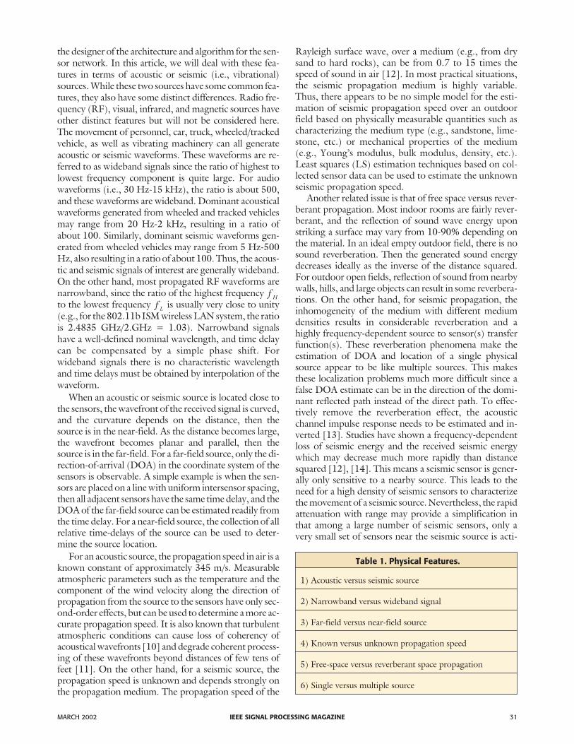
the designer of the architecture and algorithm for the sen-sor network. In this article, we will deal with these fea-tures in terms of acoustic or seismic (i.e., vibrational)sources. While these two sources have some common fea-tures, they also have some distinct differences. Radio fre-quency (RF), visual, infrared, and magnetic sources haveother distinct features but will not be considered here.The movement of personnel, car, truck, wheeled/trackedvehicle, as well as vibrating machinery can all generateacoustic or seismic waveforms. These waveforms are re-ferred to as wideband signals since the ratio of highest tolowest frequency component is quite large. For audiowaveforms (i.e., 30 Hz-15 kHz), the ratio is about 500,and these waveforms are wideband. Dominant acousticalwaveforms generated from wheeled and tracked vehiclesmay range from 20 Hz-2 kHz, resulting in a ratio ofabout 100. Similarly, dominant seismic waveforms gen-erated from wheeled vehicles may range from 5 Hz-500Hz, also resulting in a ratio of about 100. Thus, the acous-tic and seismic signals of interest are generally wideband.On the other hand, most propagated RF waveforms arenarrowband, since the ratio of the highest frequency f Hto the lowest frequency f L is usually very close to unity(e.g., for the 802.11b ISM wireless LAN system, the ratiois 2.4835 GHz/2.GHz = 1.03). Narrowband signalshave a well-defined nominal wavelength, and time delaycan be compensated by a simple phase shift. Forwideband signals there is no characteristic wavelengthand time delays must be obtained by interpolation of thewaveform.

When an acoustic or seismic source is located close tothe sensors, the wavefront of the received signal is curved,and the curvature depends on the distance, then thesource is in the near-field. As the distance becomes large,the wavefront becomes planar and parallel, then thesource is in the far-field. For a far-field source, only the di-rection-of-arrival (DOA) in the coordinate system of thesensors is observable. A simple example is when the sen-sors are placed on a line with uniform intersensor spacing,then all adjacent sensors have the same time delay, and theDOA of the far-field source can be estimated readily fromthe time delay. For a near-field source, the collection of allrelative time-delays of the source can be used to deter-mine the source location.

For an acoustic source, the propagation speed in air is aknown constant of approximately 345 m/s. Measurableatmospheric parameters such as the temperature and thecomponent of the wind velocity along the direction ofpropagation from the source to the sensors have only sec-ond-order effects, but can be used to determine a more ac-curate propagation speed. It is also known that turbulentatmospheric conditions can cause loss of coherency ofacoustical wavefronts [10] and degrade coherent process-ing of these wavefronts beyond distances of few tens offeet [11]. On the other hand, for a seismic source, thepropagation speed is unknown and depends strongly onthe propagation medium. The propagation speed of the

Rayleigh surface wave, over a medium (e.g., from drysand to hard rocks), can be from 0.7 to 15 times thespeed of sound in air [12]. In most practical situations,the seismic propagation medium is highly variable.Thus, there appears to be no simple model for the esti-mation of seismic propagation speed over an outdoorfield based on physically measurable quantities such ascharacterizing the medium type (e.g., sandstone, lime-stone, etc.) or mechanical properties of the medium(e.g., Young’s modulus, bulk modulus, density, etc.).Least squares (LS) estimation techniques based on col-lected sensor data can be used to estimate the unknownseismic propagation speed.

Another related issue is that of free space versus rever-berant propagation. Most indoor rooms are fairly rever-berant, and the reflection of sound wave energy uponstriking a surface may vary from 10-90% depending onthe material. In an ideal empty outdoor field, there is nosound reverberation. Then the generated sound energydecreases ideally as the inverse of the distance squared.For outdoor open fields, reflection of sound from nearbywalls, hills, and large objects can result in some reverbera-tions. On the other hand, for seismic propagation, theinhomogeneity of the medium with different mediumdensities results in considerable reverberation and ahighly frequency-dependent source to sensor(s) transferfunction(s). These reverberation phenomena make theestimation of DOA and location of a single physicalsource appear to be like multiple sources. This makesthese localization problems much more difficult since afalse DOA estimate can be in the direction of the domi-nant reflected path instead of the direct path. To effec-tively remove the reverberation effect, the acousticchannel impulse response needs to be estimated and in-verted [13]. Studies have shown a frequency-dependentloss of seismic energy and the received seismic energywhich may decrease much more rapidly than distancesquared [12], [14]. This means a seismic sensor is gener-ally only sensitive to a nearby source. This leads to theneed for a high density of seismic sensors to characterizethe movement of a seismic source. Nevertheless, the rapidattenuation with range may provide a simplification inthat among a large number of seismic sensors, only avery small set of sensors near the seismic source is acti-

MARCH 2002 IEEE SIGNAL PROCESSING MAGAZINE 31

Table 1. Physical Features.

1) Acoustic versus seismic source

2) Narrowband versus wideband signal

3) Far-field versus near-field source

4) Known versus unknown propagation speed

5) Free-space versus reverberant space propagation

6) Single versus multiple source

vated. This small effective seismic propagated regionmay provide a simple way to tackle the multiple sourcedetection, identification, and tracking problem basedupon simple spatial separation of these propagated re-gions [14].

Basic System FeaturesGiven the physical characteristics and features of thesources and their propagation properties consideredabove, we want to discuss the various system conceptsand features under the control of the system designer.The list in Table 2 includes power source, sensing, datatransmission, processing, and decision features used toperform source localization and beamforming. In manyfixed-site sensor network scenarios, power lines and datacable interconnections are available at all the nodes. Thus,there is essentially unlimited energy for sensing, process-ing, and decision, and reliable data transmission capabil-ity is also available. In this article, however, the sensornetwork is assumed to be ad hoc and has to work in an ar-bitrary physical environment. Thus, all operations are as-sumed to be powered by batteries of limited energy, andall data communications among the nodes are providedby low-power and low-data rate wireless RF links. Forlow-cost and low-energy consumption, we assume pas-sive sensors. These sensors only operate on the receivedacoustic and seismic waveforms from the noncooperativesource. This is in contrast to a complex active radar or so-nar system in which a very sophisticated receiver is usedto find some information of interest from the reflectedtarget return.

An important system issue is whether the sensors inthe network perform collaborative sensing of the ob-served waveforms. By this we mean information collectedby one sensor is used together with information collectedby other sensors. Clearly, this approach is more effective

than each sensor working independent of others. In thisarticle, we will assume and discuss various challenges andcosts of collaborative sensing and processing. We notethere are many degrees of collaboration. Furthermore,we can also consider whether the sensors perform syn-chronous or nonsynchronous sensing. By synchronoussensing, we mean the sensor data are collected with timetags and thus some common features at a given time in-stant can be exploited. Synchronous sensing implies tim-ing errors must be controlled. Coherent processing mustbe performed with precise synchronization. For instance,a group of sensors may perform spatial (coherent) pro-cessing to provide the source location or DOA estimate.The synchronous data must be shared within the group,but may not need to be transmitted synchronously toother parts of the network. On the contrary, noncoherentprocessing techniques may not need to share data withother sensors; thus, the synchronization requirement isrelaxed. A fully synchronous sensing system imposes con-siderable precision at the network control level as well asgreat demand on the network data transmission require-ment. The use of synchronous subarray sensing withoutrequiring full synchronous sensing of all the sensors is apractical way to attack this issue.

Another issue is whether the sensor spatial gain re-sponse is known or needs to be calibrated. Still anothersensor issue is whether the sensor locations are known.There are situations in which some of the sensor locationsare known (or estimated), other unknown sensor loca-tions can be estimated from all the sensor data [15]. All ofthese issues have great practical sensor network implica-tions with respect to collaboration.

In general, not to suffer significant degradation, com-plicated wideband array processing, beamformation, andequalization algorithms must be used to process thewideband acoustic and seismic signals of interest (see Fig.6). This means the simpler one-tap equalizer andbeamformer commonly used for narrowband RF com-munication/avionic system processing is not generally ap-plicable here. Another important system issue is whetherthe processing can be distributed to each node (or at leastat some nearby nodes) or performed at a central processornode. In the model of [16], a radio transmitting 1 kb ofdata over a distance of 100 m operating at 1 GHz using abinary phase-shift keying modulation with an error prob-ability of 10−6 and fourth-power distance loss with Ray-leigh fading, requires approximately 3 joules of energy.The same energy can then perform 300 millions instruc-tions for a 100 MIPS/watt general processor. This resultsin a ratio of 30,000 processing instructions per transmis-sion bit with equal energy consumption. Other practicalsensor networks [17] have yielded ratios in the1,000-2,000 values. These results show if the applicationand the sensor architecture permit, it is much more en-ergy efficient to perform distributed local processing thento do central processing that requires extensive communi-

32 IEEE SIGNAL PROCESSING MAGAZINE MARCH 2002

Table 2. System Features.

1) Power-line versus battery power supply

2) Wired versus wireless RF links

3) Passive versus active sensor

4) Collaborative versus noncollaborative sensing

5) Coherent versus noncoherent processing

6) Synchronous versus nonsynch. sensing

7) Known versus unknown sensor response

8) Known versus unknown sensor location

9) Wideband versus narrowband processing

10) Distributed versus central processing

cations. Of course, not all algorithms can use distributedprocessing as shown in Table 2.

Self-Organization and Ad Hoc Sensor NetworkTraditional computer/communication LAN has a fixednetwork topology and number of nodes. These networksare usually designed to maximize the throughput rate ofthe data. On the other hand, the purpose of most sensornetworks as already mentioned earlier is to detect, iden-tify, localize, beamform, and track one or more stationaryor moving sources in unknown environments. Thus, tra-ditional computer/communication network design rulesare generally not applicable here. A node is defined toconsist of one or more sensor(s) of the same type or dif-ferent types (e.g., acoustic or seismic), an associated pro-cessor, and a transceiver. These nodes can be distributedin various manners. They may be placed around the per-imeter of a plant or near the intersection of several roads(as shown in Fig. 1) in some controlled manner. Theymay be rapidly deployed by the users near the paths oftheir travel, or maybe even scattered randomly out of atruck or airplane.

Clearly to use such a sensor system, we need to havethese nodes self-organize into a usable ad hoc network inminimum time and minimum energy from some initiallygiven near-arbitrary placements [18]-[19]. After properorganization, the network should be able to pass datapackets from various nodes of the network to thenext-level user. Since the transmission and reception dis-tances of these transceivers are low, energy efficientmultihop routing needs to be used [20]. As part of themultihop routing procedure, the concept of adjacentnodes must be determined [18]. Furthermore, since theenergy used by the receiver is almost as much as that usedby the transmitter, these transceivers should be off for aslong as possible. The receiver initially listens only in somelow time duty factor manner [14]. However, when anode enters into more demanding roles, the transceivermay transmit, receive, and relay information packets inmultihop stages needing higher time duty factors.

Layered Architecture for EnergyConstraint Communication and ProcessingIn many sensor networks (e.g., AWAIRS [2]), the nodeoperates in different modes to perform different tasks,and these tasks require different power consumptions.Distinct operations of the nodes that depend on theirroles result in a layered architecture for the sensor net-work [14]. Normally, the relatively low-power sensorsand the associated electronics are always on and have theirthresholds set above some nominal ambient backgroundnoise level. When a source of sufficient strength enters thesensor network, one or more of these nodes may be trig-gered. If a sensor of a different type in the node was alsoactivated, then their combined result increases the truedetection and decreases a false detection. The processor of

these nodes may also perform the source identificationtask. Furthermore, if two or more sensors of the sametype are in the same node, then we may be able to performDOA estimation of the source from that node. We shouldnote that all these operations mentioned above are doneat the individual node level. There is no need to transmitthe raw data collected by the sensor(s) in a node to an-other node or to the next-level user. Of course, the detec-tion of a source (possibly with some information on theconfidence of the detection), the possible identification ofthe source, the DOA estimation of the source, and thetime of occurrence of these events need to be transmittedfrom each active node to the next-level user. In this case,the amount of information transmitted over the sensornetwork is relatively low. In Fig. 2, these operations areshown at the lower levels of the layered architecture la-beled intranode collaboration sensing and processing.

Various higher levels of collaborations with othernodes are possible. An activated node may inform adja-cent nodes of a recent detection to possibly lower theirthresholds to investigate the disturbing event. If the origi-nal event is not a false alarm, then other nearby sensorsshould have also detected that source. The next-level usercan then have a quite crude estimation of the location ofthe source assuming some information about the loca-tions (even if approximate) of the sensors is known. Rele-vant features extracted from sensor(s) in each node maybe sent to the next-level-user for fusion purpose to en-hance detection. One simple form of fusion is to comparethe amplitude values of different sensors (of the sametype). By using the closest-point-of-approach (CPA),which is one type of noncoherent processing, one mayprovide an estimation of the source location [21]. An-


� 1. A generic scenario of sources and sensors in a sensor network.

In many sensor networks, thenode operates in different modesto perform different tasks, andthese tasks require differentpower consumptions.

other form of fusion is to use the DOA estimate fromeach subarray of sensors of similar type. Then thetriangulation process of determining the intersection ofthese cross bearing DOA angles can be used to estimatethe source location (see the generic scenario of Fig. 1).We note in both the CPA and the DOA triangulationmethods, processing is performed locally and only smallamount of information from each node needs to be trans-mitted to the next-level user for processing. On the otherhand, for full coherent processing and beamforming ap-plications, data from selected dominant frequency bandsof interest or the whole raw data from the sensors in vari-ous relevant nodes need to be sent to other nodes or to thenext-level-user. All of these collaborations among thesensors require varying amount of costly data transmis-sion in the sensor network. These operations are shown inthe upper levels of Fig. 2 labeled internode collaborativesensing, processing, and communication.

Source Localization, DOA Estimation,and BeamformingThe earliest development of space-time processing wasspatial filtering or beamforming dating back to WorldWar II. Advances in radar, sonar, and wireless communi-cations followed using arrays of sensors. In radar andwireless communications, the information signal is mod-

ulated on the RF waveform at the transmitter and thendemodulated to a complex envelope at the receiving sen-sor. This is the narrowband signal model where the DOAinformation is contained in the phase differences amongthe sensors. The conventional beamformer is merely aspatial extension of the matched filter [22]. In classicaltime-domain filtering, the time-domain signal is linearlycombined with f i l ter ing weight to achievehigh/low/bandpass filtering. A beamformer combinesthe spatially distributed sensor collected array data lin-early with the beamforming weight to achieve spatial fil-tering. Beamforming enhances the signal from thedesired spatial direction and reduces the signal(s) fromother direction(s) in addition to possible time/frequencyfiltering. The beamformer output is a coherently en-hanced estimate of the transmitted signal, with one set ofweights for each source. In many cases, the desired signaldirection may need to be estimated.

In [22], Krim and Viberg have provided an excellent re-view and comparison of many classical and advanced para-metric narrowband techniques up to 1996. Early work inDOA estimation includes the early version of maxi-mum-likelihood (ML) solution, but it did not becomepopular due to its high computational cost. Concurrently,a variety of suboptimal techniques with reduced computa-tions have dominated the field. The more well-knowntechniques include the minimum variance method of Ca-pon [23], the multiple signal classification (MUSIC)method of Schmidt [24], and the minimum norm ofReddi [25]. The MUSIC algorithm is perhaps one of themost popular suboptimal techniques. It provides superresolution DOA estimation in a spatial pseudospectral plotby utilizing the orthogonality between the signal and noisesubspaces. However, a well-known problem with some ofthese suboptimal techniques occurs when two or moresources are highly correlated. This may be caused bymultipath or intentional jamming, and most of the

suboptimal techniques have difficul-ties without reverting to advancedprocessing or constraints. Many vari-ants of the MUSIC algorithm havebeen proposed to combat signal cor-relation and to improve performance.

Closed-Form Least SquaresSource LocalizationFor various acoustic/seismic sensorarray problems, a wideband signalmodel may be more appropriate.Since acoustic and seismic signals areunmodulated and may contain awider bandwidth, the array data isreal valued and hence thebeamforming weights are also real.In many cases we are interested in lo-cating the source in the near-field. Asthe source approaches the array, both


InternodeCollaborative

Sensing,Processing, andCommunicaton

Increasing

Node Control

IntranodeCollaborativeSensing andProcessing

Internode Beamformation andTracking Using Raw Mode Data

Fusion of Internode Data forCPA, DOA, and Tracking

Fusion of Adjacent Node Data forDetection and Identification

Intranode DOA Estimation

Fusion of Intranode Data

Intranode Processing forDetection and Identification

Continuous Sensing and “Tripwire”Threshold Detection

Sensor Network Output(s)or Activate Above Layer(s)

IncreasingPerformance

andIncreasing

PowerConsumption

� 2. Layered architecture showing increasing communication, computation, and energy cost.

The purpose of a sensor networkis to monitor an area, includingdetecting, identifying, localizing,and tracking one or more objectsof interest.

the angle and range become parameters of interest. Notethat unlike the radar and communications problemswhere the signal may be a random process with knownstatistics or drawn from a known finite alphabet, theacoustic/seismic source signals are most likely to be deter-ministic but unknown (e.g., waveform generated by apassing vehicle). An additional factor that arises in thenear-field scenario is that each sensor may have a differentgain as opposed to equal gain in the far-field case. Thesensors are assumed to be omnidirectional, and the gainvariation is due to differences in the propagation paths inthe near-field geometry. For a randomly distributed arrayof R sensors, the data collected by the pth sensor at time ncan be given by

( )x n a s n t w np pm

m

Mm

pm

p( ) ( ),( ) ( ) ( )= − +=

∑1

0 (1)

for n L p R= − =0 1 1, , , , , ,K K and m M=1, ,K , where M isthe number of sources ( M R< ), a p

m( ) is the signal gainlevel of the mth source at the pth sensor (assumed to beconstant within the block of data), s m

0( ) is the source sig-

nal, t pm( ) is the fractional time-delay in samples (which is

allowed to be any real-valued number), and w p iszero-mean white Gaussian noise with variance σ2 . Thetime-delay is defined by t vp

ms pm

( ) / ,= −r r where r s mis

the mth source location, r p is the pth sensor location, andv is the speed of propagation in length unit per sample.Define the relative time-delay between the pth and the qthsensors by

( )t t t vpqm

pm

qm

s p s qm m

( ) ( ) ( ) / .= − = − − −r r r r

Note, in the wideband problem, time delays are exploitedas opposed to phase differences in thenarrowband case.

One class of near-field source localization al-gorithm is based first on using time-delay tech-niques. These algorithms provide closed-formsolutions to estimate the location of a singlesource based on spherical intersection [26], hy-perbolic intersection [27], or linear intersection[28], from the measured relative time-delays.Nevertheless, these algorithms require knownspeed of propagation. In [4] and [29], aclosed-form LS and constrained least-squares(CLS) solutions are derived for unknown speedof propagation. The CLS solution improves thelocation estimate from that of the LS solutionby forcing an equality constraint on two compo-nents of the solution. The closed-form sourcelocation estimate is given by the solution of a setof linear equations [29], expressed as

Ay b= , (2)

where the system matrix A contains the sensorlocations and relative time delays, the un-

known vector y contains the source location, sourcerange, and the speed of propagation, and the vector b is afunction of sensor locations. An overdetermined LS solu-tion can be given by evaluating the pseudoinverse A † ofthe matrix A in the case of six or more sensors (forthree-dimensional (3-D) localization) resulting iny A b= † . The earliest time-delay estimation is based onmaximizing the cross-correlation between sensor data[30]. Other phase transform (PHAT) methods [31] orsecond-order subspace methods [4] have been proposedto improve time-delay estimation under Gaussian noiseassumption. Other robust time-delay estimation meth-ods have been proposed for impulsive noise with“heavy-tailed” distribution [32], and higher-order statis-tics have even been exploited to estimate time-delays ofmultiple sources [33].

Iterative Maximum-Likelihood SourceLocalization and DOA EstimationAnother class of source localization algorithm is based onparameter estimation, where only iterative solutions areavailable. Despite the possible increase in computationalcomplexity, this class of algorithms generally offersgreater estimation accuracy. The fundamental differencebetween the parametric and closed-form solutions de-pends on the use of the optimization criterion. Theclosed-form solution is indeed optimized in two inde-pendent steps, namely, estimating relative time delays be-tween sensor data and then source location based on thetime-delay estimates. On the other hand, the parametricsolution, which is based on the maximum-likelihood cri-terion, is optimized in a single step directly from the datawithout needing time-delay estimation. The parametricML method has been shown to outperform the closed-


10

5

0

−5

X-Axis (m)(a)

X-Axis Position (m)(b)

−8

−8

−6

−6

−4

−4

−2

−2

0

0

2

2

4

4

6

6

Y-A

xis

(m)

Sensor LocationsSource True Track

MusicLSMLCRB

2

1.5

1

0.5

0

Sou

rce

Loca

lizat

ion

RM

S E

rror

(m

)

� 3. (a) A moving source scenario with five sensors; (b) source localization RMSerror comparisons.

form methods [15] for the single source case. In the caseof multiple sources, using even more advanced time-delayestimation techniques, the closed-form methods do notseem to guarantee solutions in all cases. Thus, theclosed-form methods in general cannot estimate multiplesource locations, while the parametric method can do soby expanding the parameter space.

To obtain the parametric solution, it is best to trans-form the wideband data to the frequency-domain, wherea narrowband signal model can be given for each fre-quency bin. A block of L samples is collected from eachsensor and transformed to the frequency-domain by a dis-crete Fourier transform of length N. In the frequency do-main, the array signal spectrum vector is given by X( )k ,which contains the phase-shifted (a function of source lo-cation or DOA) version of the source signal spectrumplus the noise spectrum vector, for k N= −0 1, ,K . Thenoise spectrum vector is zero-mean complex whiteGaussian distributed with variance Lσ2 . By combiningthe data spectrum vectors in the positive frequency bins,the ML solution can be given by

arg max ( , ) ( )/

ΘΘP k X k

k

N2

1

2

=∑ ,

(3)

where Θ is the unknown parameter vector which may ei-ther be the source locations or the DOAs, and P k( , )Θ is anorthogonal projection matrix [15]. An efficient alternat-ing projection (AP) procedure was proposed in [15] forthe ML method to avoid a multidimensional search by se-quentially estimating the location of one source while fix-ing the estimates of other source locations from theprevious iteration. Once the source locations are esti-mated, the ML estimate of the source signals (MLbeamformer output) can be obtained. It is interesting tonote that in the near-field case, the ML beamformer out-put is the result of forming a focused spot (or area) on thesource location rather than a beam since range is also con-sidered. Another possible parametric solution is thewideband extension of the MUSIC algorithm; however,it has been shown to be highly suboptimal in thenear-field case [15].

Cramér-Rao Bound AnalysisBesides the development of the estimation algorithms, itis useful to consider their theoretical performance limits.The Cramér-Rao bound (CRB) is a well-known statisti-cal method to obtain the theoretical lower bound of theestimation variance for the performance of any unbiasedestimator [34]. The CRBs for DOA and source localiza-tion are derived based on the time-delay model in [35],and the CRBs based on the data model of (1) are given in[15]. More physical properties of the problem can befound from the CRBs based on the data model. In partic-ular, the source localization variance, denoted as the vari-ance matrix Σ, is lower bounded by the CRB, i.e.,Σ≥G / S, which can be broken down into two separateparts, a scalar factor S that depends only on the signal anda matrix G that depends only on the array geometry. Thissuggests separate performance dependence of the signaland the geometry. Thus, for any given signal, the CRBcan provide the theoretical performance of a particulargeometry and helps the design of an array configurationfor a particular scenario of interest. The signal depend-ence part shows that theoretically the source locationRMS error is linearly proportional to the noise level andspeed of propagation and inversely proportional to thesource spectrum and frequency. Thus, better source loca-tion estimates can be obtained for high frequency signalsthan low frequency signals. In further sensitivity analysis,large range estimation error is found when the source sig-nal is unknown, but such unknown parameter does notaffect the angle estimation.

Simulation and Experimental ResultsConsider the simulation of a moving source on a straightline near a circular array of five sensors as shown in Fig.3(a). At each position, the array data is simulated using an


4.5

4

3.5

3

2.5

2

1.5

1

0.5

0

Y-A

xis

(m)

Sensor LocationsActual Source LocationSource Location Estimates

−2 −1 0 1 2 3 4X-Axis (m)

� 4. Localization of an indoor near-field source using the LSmethod.

0

Y-A

xis

(m)

−5X-Axis (m)

2

4

6

8

10

12

14

16

0 5 10

Source 1

Source 2

Sensor LocationsActual Source LocationsSource Location Estimates

� 5. Two-source localization via bearing crossing of the DOAs ob-tained by the ML alternating projection method.

acoustic waveform of a measured vehicle signature. Thespeed of propagation is assumed to be 345 m/s. In Fig.3(b), the source localization RMS errors are plotted us-ing the wideband MUSIC, LS, and ML algorithms andthe CRB. Both the LS and ML algorithms are shown toapproach the CRB asymptotically, but the ML algorithmuniformly outperforms the LS algorithm. However, thewideband MUSIC yields much worse estimates thanthose of the LS and ML methods, especially when thesource is far from the array.

To demonstrate the usefulness of the localization algo-rithms, an experiment was conducted inside asemi-anechoic chamber where six microphones simulta-neously collect the sound (prerecorded moving lightwheeled vehicle) driven by an omni-directional loudspeaker placed in the middle of the room. As depicted inFig. 4, the location of the sound source can be estimatedwith high accuracy (RMS error of 127 cm) using the LSalgorithm under 12 dB SNR. For the same data set, theML algorithm can even improve the accuracy to an RMSerror of 73 cm. Then, another experiment was conductedoutdoor with two linear arrays collecting the sound (twodistinct prerecorded moving light wheeled vehicles) si-multaneously coming from two different omni-direc-tional loud speakers placed between the two arrays. TheDOAs of the two sources are separately estimated for thetwo arrays using the ML alternating projection algo-rithm. The source locations are then estimated via the tri-angulation of bearing crossings of the DOAs. In Fig. 5,accurate location estimates (RMS error of 36 cm forsource 1 and RMS error of 45 cm for source 2) are shownfor the dataset with 11 dB SNR. In this case, the closed-form methods have difficulties separating the time-delays ofthe two sources.

Blind BeamformingDespite the existence of many calibrating tech-niques, another approach in array signal process-ing is blind beamforming. In general, blindbeamforming is an operation similar to conven-tional beamforming except without the knowl-edge of sensor responses and locations. In otherwords, blind beamforming enhances the signalby processing only the array data without muchinformation about the array. A cumulant-basedblind beamforming algorithm was proposed in[36] for the narrowband problem. Thecumulant, or the higher order statistics (HOS),of the data is utilized to estimate the steering vec-tor of the source up to a scale factor. This can beviewed as a form of online calibration usingHOS, which often requires longer data lengths.In some practical scenarios, the data length needsto be quite short for a moving source.

Another blind beamforming that uses the sec-ond-order statistic (SOS) was proposed in [4]for wideband signals. A tap delay line of weights

is applied to each sensor to perform space-time process-ing as depicted in Fig. 6. The blind maximum power(MP) beamformer in [4] obtains array weights from thedominant eigenvector (or singular vector) associatedwith the largest eigenvalue (or singular value) of thespace-time sample correlation (or data) matrix. This ap-proach not only collects the maximum power of the dom-inant source, but also provides some rejection of otherinterferences and noise. Theoretical justification of thisapproach uses a generalization of Szegö theory of the as-ymptotic distribution of eigenvalue of the Toeplitz form.The relative phase information among the weights yieldsthe relative propagation time delays from the dominantsource to the array sensors. We should also mention con-siderable blind beamforming, source localization, andtracking results from measured seismic sources requiringinternode collaboration have also been reported [37].

ConclusionsResearch in distributed sensor network requires integrat-ing multidisciplinary concepts and technologies frommany areas. In signal processing, various sensor arrayprocessing algorithms and concepts have been adopted,but must be further tailored to match the communicationand computational constraints. With advances in inte-


In many sensor networks, thenode operates in different modesto perform different tasks andthese tasks require differentpower consumptions.

Wavefrontsfrom Source 1

Wavefrontsfrom Source 2

x n1( )

x n2( )x n3( )w n* ( )10

w n* ( )11

w n* ( )1( 1)L−

w n* ( )20

w n* ( )21

w n* ( )2( 1)L−

w n* ( )30

w n* ( )31

w n* ( )3 ( 1)L−

y n( ), Filtered Output Signal

∆ ∆ ∆

∆ ∆ ∆

∆ ∆ ∆

+ + +

+

+

+ +

� 6. Block diagram of blind beamforming with two sources and three sensors.

grated cuircuit technology, the processing power of thenode constantly improves, thus allowing the use of morecomputationally demanding optimal signal processing al-gorithms. With advances in wireless radio hardware andsoftware network protocol and control, reliably move-ment of sensor data for demanding processing algorithmsbecomes feasible. However, concerns of instantaneouspower and total energy for computations and communi-cations of battery-driven sensor network are always pres-ent. These factors influence greatly the intra- andinternode collaboration and the relevant signal and arrayprocessing algorithms and architectures. Active researchproblems remain for the design of sensor array algo-rithms that are robust and adaptive to environmentalchanges and under demanding weather, wind, reverbera-tion, impulsive noise, and strong interference conditions.While analytical algorithmic development and verifica-tion by simulations are important, reliable measured sen-sor array data taken over realistic field conditions underappropriate applications are crucially needed to truly ver-ify and test these concepts and algorithms. It is onlythrough alternating series of designs, tests, and verifica-tions can the full potentials of the sensor network arraysbe realized.

AcknowledgmentsThis work is partially supported by DARPA-ITO SensITprogram under contract N66001-00-1-8937 andAROD-PSU contract S01-26.

Joe C. Chen received the B.S. (with honors) and M.S. de-grees in electrical engineering from the University of Cal-ifornia at Los Angeles (UCLA), in 1997 and 1998,respectively. He is currently a Raytheon Fellow pursuingthe Ph.D. degree in electrical engineering at UCLA.Since 1997, he has been with the Sensors and ElectronicsSystems group of Raytheon Systems Company (formerlyHughes Aircraft Company) in El Segundo, CA. He hasalso been a Research Assistant at UCLA since 1998 and aTeaching Assistant since 2001. His research interests in-clude estimation theory and statistical signal processing asapplied to sensor array processing, source localization,multichannel system identification and deconvolution,and radar systems. He is a member of Tao Beta Pi and EtaKappa Nu and a Student Member of the IEEE.

Kung Yao received the B.S.E., M.A., and Ph.D. degreesin electrical engineering from Princeton University,Princeton, NJ. He has worked at the Princeton-Penn Ac-celerator, the Brookhaven National Lab, and the BellTelephone Labs, Murray Hill, NJ. He was a NAS-NRCPost-Doctoral Research Fellow at the University of Cali-fornia, Berkeley. He was a Visiting Assistant Professor atthe Massachusetts Institute of Technology and a VisitingAssociate Professor at the Eindhoven Technical Univer-sity. In 1985-1988, he was an Assistant Dean of the

School of Engineering and Applied Science at UCLA.Presently, he is a Professor in the Electrical EngineeringDepartment at UCLA. His research interests include sen-sor array systems, digital communication theory and sys-tems, wireless radio systems, chaos communications andsystem theory, and digital and array signal and array pro-cessing. He has published more than 250 papers. He re-ceived the IEEE Signal Processing Society’s 1993 SeniorAward in VLSI Signal Processing. He is the co-editor ofHigh Performance VLSI Signal Processing (IEEE Press,1997). He was on the IEEE Information Theory Soci-ety’s Board of Governors and is a member of the SignalProcessing System Technical Committee of the IEEESignal Processing Society. He has been on the editorialboards of various IEEE Transactions, with the most re-cent being IEEE Communications Letters. He is a Fellowof the IEEE.

Ralph E. Hudson received his B.S. in electrical engineeringfrom the University of California at Berkeley in 1960 andthe Ph.D. degree from the U.S. Naval PostgraduateSchool, Monterey, CA, in 1969. In the U.S. Navy, he at-tained the rank of Lieutenant Commander and servedwith the Office of Naval Research and the Naval Air Sys-tems Command. From 1973-1993, he was with HughesAircraft Company, and since then he has been a ResearchAssociate in the Electrical Engineering Department ofthe University of California at Los Angeles. His researchinterests include signal and acoustic and seismic arrayprocessing, wireless radio, and radar systems. He receivedthe Legion of Merit and Air Medal and the Hyland PatentAward in 1992.

References[1] K. Bult, et al., “Wireless integrated microsensors,” in Proc. Tech. Dig.

Solid-State Sensor and Actuator Workshop, June 1996, pp. 205-210.

[2] J.R. Agre, L.P. Clare, G.J. Pottie, and N.P. Romanov, “Development plat-form for self-organizing wireless sensor networks,” in Proc. SPIE, vol. 3713,Mar. 1999, pp. 257-268.

[3] L.P. Clare, G.J. Pottie, and J.R. Agre, “Self-organizing distributed net-works,” in Proc. SPIE, vol. 3713, Mar. 1999, pp. 229-237.

[4] K. Yao, R.E. Hudson, C.W. Reed, D. Chen, and F. Lorenzelli, “Blindbeamforming on a randomly distributed sensor array system,” IEEE J. Se-lect. Areas Commun., vol. 16, pp. 1555-1567, Oct. 1998.

[5] J.M. Kahn, R.H. Katx, and K.S.J. Pister, “Next century challenges: Mobilenetworking for ‘Smart Dust’,” in Proc. Mobicom, 1999, pp. 483-492.

[6] D. Estrin and R. Govindan, “Next century challenges: scalable coordinationin sensor networks,” in Proc. Mobicom, 1999, pp. 263-270.

[7] A.P. Chandrakasan, et al., “Design consideration for distributedmicrosensor system,” in Proc. CICC, 1999, pp. 279-286.

[8] S. Kumar and D. Shepherd, “SensIT: sensor information technology forthe warfighter,” in Proc. ISIF, Aug. 2001, pp. TuC1: 3-9.

[9] ARL Federated Laboratory Advanced Sensor Program. Available:http://www.arl.army.mil/alliances

[10] D.K. Wilson, “Performance bounds for acoustic direction of arrival raysoperating in atmospheric turbulence,” J. Acousti. Soc. Amer., vol. 103, pp.1306-19, 1998.


[11] T. Pham, ARL Laboratory, private communication.

[12] P. Kearey and M. Brooks, An Introduction to Geophysical Exploration, 2nded. Oxford, U.K.: Blackwell, 1994, pp. 26-27.

[13] S. Affes and Y. Grenier, “A signal subspace tracking algorithm for micro-phone array processing of speech,” IEEE Trans. Speech Audio Processing, vol.5, pp. 425-437, Sept. 1997.

[14] J. Agre and L. Clare, “An integrated architecture for cooperative sensingnetworks,” Computer, vol. 33, pp. 106-8, May 2000.

[15] J.C. Chen, R.E. Hudson, and K. Yao, “Joint maximum-likelihood sourcelocalization and unknown sensor location estimation for near-fieldwideband signals,” in Proc. SPIE, vol. 4474, Jul. 2001.

[16] G.J. Pottie and W.J. Kaiser, “Wireless integrated network sensors,”Comm. ACM, vol. 43, pp. 51-58, May 2000.

[17] M. Srivastava, UCLA, private communication.

[18] K. Sohrabi, J. Gao, V. Ailawadhi, and G.J. Pottie, “Protocols forself-organization of a wireless sensor network,” IEEE Personal Commun.,vol. 7, pp. 16-27, Oct. 2000.

[19] A. Wang and A. Chandrakasan, “Energy efficient system partitioning fordistributed wireless sensor networks,” in Proc. IEEE ICASSP, vol. 2, May2001, pp. 905-908.

[20] C. Schurgers and M. Srivastava, “Energy conserving routing in sensor net-works,” in Proc. IEEE Milcom, Nov. 2001.

[21] D. Li, K. Wong, Y.H. Hu, and A. Sayeed, “Detection, classification andtracking in distributed sensor networks,” in Proc. ISIF, Aug. 2001, pp.TuC2: 3-9.

[22] J. Krim and M. Viberg, “Two decades of array signal processing research:The parametric approach,” IEEE Signal Processing Mag., vol. 13, pp. 67-94,Jul. 1996.

[23] J. Capon, “High-resolution frequency-wavenumber spectrum analysis,”Proc. IEEE, vol. 57, pp. 2408-2418, Aug. 1969.

[24] R.O. Schmidt, “Multiple emitter location and signal parameter estima-tion,” IEEE Trans. Antennas Propagat., vol. AP-34, pp. 276-280, Mar.1986.

[25] S.S. Reddi, “Multiple source location—A digital approach,” IEEE Trans.Aerospace Electronics Syst., vol. AES-15, pp. 95-105, Jan. 1979.

[26] J.O. Smith and J.S. Abel, “Closed-form least-squares source location esti-mation from range-difference measurements,” IEEE Trans. Acoustics, Speech,Signal Processing, vol. ASSP-35, pp. 1661-9, Dec. 1987.

[27] Y.T. Chan and K.C. Ho, “A simple and efficient estimator for hyperboliclocation,” IEEE Trans. Signal Processing, vol. 42, pp. 1905-1915, Aug.1994.

[28] M.S. Brandstein, J.E. Adcock, and H.F. Silverman, “A closed-form loca-tion estimator for use with room environment microphone arrays,” IEEETrans. Speech Audio Processing, vol. 5, pp. 45-50, Jan. 1997.

[29] J.C. Chen, K. Yao, R.E. Hudson, T.L. Tung, C.W. Reed, and D. Chen,“Source localization of a wideband source using a randomly distributedbeamforming sensor array,” in Proc. ISIF, Aug. 2001, pp. TuC1: 11-18.

[30] G.C. Carter, Ed., Coherence and Time Delay Estimation. New York: IEEEPress, 1993.

[31] P.A. Petropulu and C.L. Nikias, Higher Order Spectral Analysis: A Nonlin-ear Signal Processing Framework. Englewood Cliffs, NJ: Prentice Hall,1993.

[32] X. Ma and C.L. Nikias, “Joint estimation of time delay and frequency de-lay in impulsive noise,” IEEE Trans. Signal Processing, vol. 44, pp. 2669-87,Nov. 1996.

[33] B. Emile, P. Common, and J. Le Roux, “Estimation of time-delays withfewer sensors than sources,” IEEE Trans. Signal Processing, vol. 46, pp.2012-15, July 1998.

[34] S.M. Kay, Fundamentals of Statistical Signal Processing: Estimation Theory.Englewood LCiffs, NJ: Prentice-Hall, 1993.

[35] C.W. Reed, R. Hudson, and K. Yao, “Direct joint source localization andpropagation speed estimation,” in Proc. IEEE ICASSP, vol. 3, Mar. 1999,pp. 1169-1172.

[36] M.C. Dogan and J.M. Mendel, “Cumulant-based blind optimumbeamforming,” IEEE Trans. Aerospace Electronic Syst., vol. 30, pp. 722-741,Jul. 1994.

[37] K. Yao, R.E. Hudson, C.W. Reed, T.L. Tung, D. Chen, and J.C. Chen,“Estimation and tracking of an acoustic/seismic source using abeamforming array based on residual minimizing methods,” in Proc.IRIA-IRIS 1999 Meeting, Jan. 2000, pp. 153-163.


source localization and beamforming d - computer...

Documents