source location of forced oscillations using … location of forced oscillations using synchrophasor...

Source Location of Forced Oscillations

Using Synchrophasor and SCADA Data

James G O’Brien

Pacific Northwest National

Laboratory

Richland WA

[email protected]

Tianying Wu Washington State University

Pullman WA

[email protected]

Vaithianathan “Mani”

Venkatasubramanian Washington State University

Pullman WA

[email protected]

Hongming Zhang Peak Reliability

Loveland CO

[email protected]

Abstract1

Recent advances in synchrophasor based

oscillation monitoring algorithms have allowed

engineers to detect oscillation issues that may have

previously gone undetected. Although such an

oscillation can be flagged and its oscillation shape can

indicate the general vicinity of its source, low number

of synchrophasors means that a specific generator or

load that is the root cause of an oscillation cannot

easily be pinpointed. Fortunately, SCADA serves as a

much more readily available telemetered source of

data if only at a relatively low sampling rate of 1

sample every 1 to 10 seconds. This paper shows that it

is possible to combine synchrophasor and SCADA data

for effective source location of forced oscillations. For

multiple recent oscillation events, the proposed

automatic methods were successful in correct

identification of the oscillation source which was

confirmed in each case by discussion with respective

generation plant owners.

1. Introduction

Different from the natural electromechanical modal

oscillations, forced oscillations in power systems are

caused by external sources such as cyclic loads and

control failures in generator sites [1],[2]. The

identification of these forced oscillations has been a

significant problem for the industry. Because of the

increase in PMU visibility, there is significant work

being done in detecting and locating forced oscillations

using synchrophasor measurements [3]-[6]. The source

location becomes difficult especially when there is

resonance between the forced oscillation and a system

1 The author James O’Brien was with Peak Reliability while

doing the research reported in this paper.

inter-area mode [6] which will not be discussed in this

paper.

However, the observability of oscillation sources

using PMU data is less than ideal. Even though many

hundreds of PMUs have been installed across the

power grid in North America, most of these are located

for monitoring transmission corridors and do not

provide much coverage of generation facilities.

Therefore, the indication from the oscillation shapes

produced by oscillation detection software that uses

PMU data is not specific enough for source location of

problematic oscillations. In our experience, oscillation

shape from PMU data analysis typically points towards

a portion of the system with dozens of candidate

generation sites. With low PMU visibility, source

location of forced oscillations becomes difficult to

produce tangible results without exhaustive manual

analysis.

Typically, other sources of data need to be

examined for their use in this application. The most

readily available source is the SCADA data that is

received throughout the western interconnection

(commonly referred to as Western Electricity

Coordinating Council (WECC) power system) by Peak

Reliability. Currently while we only have PMU

visibility of tens of generators in the WECC system,

the SCADA visibility covers more than 2000

generators. Both real and reactive power outputs are

monitored from each generator.

Due to the low sampling rate of SCADA data and

its non-synchronized nature, it is a technical challenge

to detect forced oscillations using SCADA data.

However, once a possible forced oscillation has been

detected with PMU measurements, SCADA data can

then be used for locating the specific source. As an

example, the plot below shows the analog frequency

chart recording of an oscillation event in 1992 [7] that

lasted for about 38 minutes. Note that the difference

between normal ambient conditions versus sustained

oscillations is clearly observable in Figure 1 even

3173

Proceedings of the 50th Hawaii International Conference on System Sciences | 2017

URI: http://hdl.handle.net/10125/41541ISBN: 978-0-9981331-0-2CC-BY-NC-ND

mailto:[email protected]




though the 1 Hz oscillations were much faster than the

slow time response of the analog recorder.

The challenge then becomes how to properly

identify from the multitude of SCADA data such

distinctly different responses between when the

oscillations of interest are present versus when they are

not. This paper proposes two strategies for

automatically selecting and ranking likely generator

oscillation sources from their recorded SCADA

measurements. Synchrophasor based oscillation

monitoring is used first to estimate the onset of a

forced oscillation so that the distinction between

ambient and oscillation conditions can be made.

Oscillation shape of the forced oscillation from

synchrophasors can also be used to validate the results

of SCADA based ranking in most cases excepting

when inter-area resonance is in effect [6].

Figure 1. MW chart record of the Rush Island

event on June 12, 1992 [7]

In this paper, two slightly different methods are

proposed in order to locate the sources of forced

oscillations using SCADA data. One is denoted Pattern

Mining Algorithm (PMA), which considers the number

of high-amplitude peaks in SCADA data during the

time periods when oscillations were detected by the

PMU engines as the key factor in ranking. The second

one is called Maximal Variance Ratio Algorithm

(MVRA) which ranks the SCADA signals based on the

ratio of the average variances during oscillation and

ambient time periods. The two methods serve to cross-

check the ranking with each other.

The rest of the paper is organized as follows:

Section 2 introduces a recent oscillation event in

western interconnection power system, which

motivated this paper. The two methods of locating the

sources of forced oscillations using SCADA data are

then proposed in Section 3, and are illustrated on the

event in Section 2. In Section 4, two other oscillation

events are studied. Section 5 concludes the paper.

2. Event 1 on January 27, 2015

A recent oscillation event (denoted Event 1)

occurred on January 27, 2015 in western

interconnection power system. It has been detected

during offline studies using Fast Frequency Domain

Decomposition (FFDD) algorithm [8].

As shown in Figure 2(a), the oscillation started at

approximately 11:00 AM and lasted till about 11:40

AM according to FFDD analysis of the WECC PMU

data. Analysis window length for FFDD was 180

seconds which was updated every 10 seconds in a

moving window formulation [8]. The oscillation

frequency was at around 1.12 Hz with the damping

ratio estimated to be below 1%. Figure 2(b) shows the

average oscillation shape for the 1.12 Hz oscillation of

Figure 2(a). PMU signals with the largest oscillation

shape magnitudes were all from the same area, with

low PMU coverage consisting of more than 50

generation substations. The presence of the forced

oscillation can be clearly seen in the line current

measurement from one of the PMUs in Figure 2(c).

Although the oscillation magnitude is small, the FFDD

algorithm [8] can detect it well as shown in the

summary plot Figure 2(a).

(a) Summary plot (b) Oscillation shape

(c) Line current measured by one PMU

Figure 2. Detection of the forced oscillation using

FFDD

In order to identify the specific source of the forced

oscillation, three-hour SCADA data (9:30 AM to 12:30

PM) recorded from over 2000 generators in western

interconnection power system was used for analysis.

The discussion in this paper assumes the oscillation

source to be a generator while similar analysis can be

applied for load sources as well.

3174

Because of the vast amount of SCADA data, even

with the indication from oscillation shape results, it

took several weeks to identify the oscillation source

through the manual search process. Subsequently,

efficient methods have been developed for locating the

source of forced oscillations automatically from among

thousands of SCADA signals.

3. Use of SCADA data for source location

Unlike the high sampling rate PMU data, the

SCADA system only provides data from generators

and substations every 1 to 10 seconds. Measurement

and collection of SCADA data are not time-

synchronized. Therefore, SCADA data has been first

interpolated like a synchronized stream of data with

one sample every 10 seconds. The sampling rate then

becomes 0.1 Hz which suggests that the corresponding

Nyquist frequency is 0.05 Hz. It is a challenge to

analyze a forced oscillation at 1.12 Hz of Event 1 with

such low sampling rate data using any existing signal

processing technique.

Another challenge in using SCADA data is that the

signals are recorded with different resolutions (tenth of

MW or MVAR for some channels, and one MW or

MVAR for some channels). Moreover, the sensitivities

of the signals vary a lot in different areas of the system.

Therefore, some of the signals can be very noisy,

whereas others may remain unchanged for long

periods.

Two methods that can handle all these practical

issues are proposed in this section. Purely from the

very large number of generators in a large power

system, it is very difficult to identify the oscillation

source effectively while avoiding false alarms. For this

purpose, the two slightly different methods can be used

to reinforce the ranking of possible source locations.

The start and end time of the forced oscillation

need to be known from a PMU based oscillation

detection engine such as by using FFDD of [8] before

applying these two methods to the SCADA data. The

time window in between the start and end times of

oscillation detection will be referred to as the

oscillation window for the rest of the paper. Non-

oscillation time period is accordingly referred to as the

ambient window. The oscillation window of Event 1 in

Section II is from 11:00 AM to 11:40 AM.

In order to properly distinguish from a generator

which shows oscillating characteristics within the

oscillation window, versus another generator that has

these characteristics throughout the entire data set, an

initial ambient window is needed for baselining.

Both methods will compute the ranking index for

all the generator outputs, where n is the number of

channels.

3.1. Pattern Mining Algorithm (PMA)

To begin with, the data goes through a pre-

screening process (denoted the data sanity check) to

ensure that the generator is in use and there is some

minimum variation within the output for the set. The

channel whose maximal output is less than 10 MW or

MVAR, and the one whose maximal difference for the

entire data set is less than 1 MW or MVAR are

ignored.

Next, a 25-point median filter is applied for

detrending. The absolute values of the differences

between the raw measurements and the filtered data,

denoted the detrended data, can be used as a measure

of the oscillation activity as seen in the SCADA signal.

When an oscillation occurs, the amplitude of the

differences during the oscillation window should be

relatively higher than the amplitudes during the

ambient window. Accordingly, a threshold is needed in

order to rule out small differences. The threshold

(denoted the 3σ threshold) is set to be three times the

standard deviation of the detrended data in the ambient

window.

This method then counts the number of the high-

amplitude peaks in the raw measurements whose

detrended values are outside the 3σ threshold in the

oscillation window, denoted NUMosc, and in the

ambient window, denoted NUMamb. In this context, the

amplitude of the peaks is ignored per se. The ranking

index of each channel is then formulated as,

_ _

_ , 1, 2, , ,osc i amb i

PMA i

osc amb

NUM NUMK i n

Length Length (1)

where Lengthosc and Lengthamb represent the lengths

(total number of samples) of the oscillation and the

ambient windows, respectively.

In order to determine relative ranking between the

generators, the main steps of the pattern mining

algorithm are summarized as below.

1) Input SCADA data of generators and the oscillation

event time as detected by FFDD using PMU data.

2) Data sanity check.

3) Apply the median filter and subtract the median

filtered data from the raw data for detrending.

4) Calculate the absolute values of the differences

between the raw measurements and the filtered data.

5) Reject the channel if the maximal absolute value of

the differences is less than 1 MW or MVAR.

6) Count NUMosc_i and NUMamb_i.

7) Compute the ranking index KPMA_i based on (1).

3175

8) Apply step 2 to 7 for the rest of channels.

9) Select Top 3 channels based on the ranking index.

10) Inspect the MW outputs of the possible oscillation

sources for manual verification.

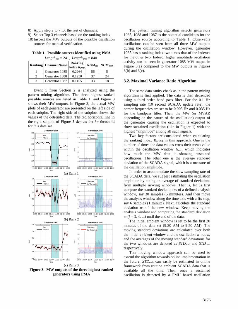
Table 1. Possible sources identified using PMA

Lengthosc = 241, Lengthamb = 840.

Ranking Channel Name Ranking

Index KPMA NUMosc NUMamb

1 Generator 1085 0.2264 56 5

2 Generator 1088 0.1250 37 24

3 Generator 1087 0.1155 33 18

Event 1 from Section 2 is analyzed using the

pattern mining algorithm. The three highest ranked

possible sources are listed in Table 1, and Figure 3

shows their MW outputs. In Figure 3, the actual MW

plots of each generator are presented on the left side of

each subplot. The right side of the subplots shows the

values of the detrended data. The red horizontal line in

the right subplot of Figure 3 depicts the 3σ threshold

for this data set. Generator 1085

Time

MW

09:30 10:00 10:30 11:00 11:30 12:00 12:30200

225

250

275

300

325

350

Raw

Filtered

Generator 1085

Time

MW

09:30 10:00 10:30 11:00 11:30 12:00 12:30-3

0

3

6

9

12

15

18

Difference

3 Threshold

(a) Rank 1

Generator 1088

Time

MW

09:30 10:00 10:30 11:00 11:30 12:00 12:30710

715

720

725

730

735

Raw

Filtered

Generator 1088

Time

MW

09:30 10:00 10:30 11:00 11:30 12:00 12:30-1

0

1

2

3

4

5

6

7

Difference

3 Threshold

(b) Rank 2 Generator 1087

Time

MW

09:30 10:00 10:30 11:00 11:30 12:00 12:30690

700

710

720

730

740

Raw

Filtered

Generator 1087

Time

MW

09:30 10:00 10:30 11:00 11:30 12:00 12:30-2

0

2

4

6

8

10

12

Difference

3 Threshold

(c) Rank 3

Figure 3. MW outputs of the three highest ranked

generators using PMA

The pattern mining algorithm selects generators

1085, 1088 and 1087 as the potential candidates for the

oscillation source according to Table 1. Observable

oscillations can be seen from all three MW outputs

during the oscillation window. However, generator

1085 has a ranking index two times that of the indexes

for the other two. Indeed, higher amplitude oscillation

activity can be seen in generator 1085 MW output in

Figure 3(a) compared to the MW outputs in Figures

3(b) and 3(c).

3.2. Maximal Variance Ratio Algorithm

The same data sanity check as in the pattern mining

algorithm is first applied. The data is then detrended

using a third order band pass filter. For the 0.1 Hz

sampling rate (10 second SCADA update rate), the

corner frequencies are set to be 0.005 Hz and 0.035 Hz

for the bandpass filter. Then, the MW (or MVAR

depending on the nature of the oscillation) output of

the generator causing the oscillation is expected to

show sustained oscillation (like in Figure 1) with the

highest “amplitude” among all such signals.

Two key factors are considered when calculating

the ranking index KMVRA in this approach. One is the

number of times the data values cross their mean value

within the oscillation window Nosc, which indicates

how much the MW data is showing sustained

oscillations. The other one is the average standard

deviation of the SCADA signal, which is a measure of

the oscillation amplitude.

In order to accommodate the slow sampling rate of

the SCADA data, we suggest estimating the oscillation

amplitude by taking an average of standard deviations

from multiple moving windows. That is, let us first

compute the standard deviation σ1 of a defined analysis

window, say 30 samples (5 minutes). And then move

the analysis window along the time axis with a fix step,

say 6 samples (1 minute). Next, calculate the standard

deviation σ2 of the new window. Keep moving the

analysis window and computing the standard deviation

σi (i = 3, 4, ...) until the end of the data.

The initial ambient window is set to be the first 20

minutes of the data set (9:30 AM to 9:50 AM). The

moving standard deviations are calculated over both

the initial ambient window and the oscillation window,

and the averages of the moving standard deviations for

the two windows are denoted as STDamb and STDosc,

respectively.

This moving window approach can be used to

extend the algorithm towards online implementation in

the future. STDamb can easily be estimated in online

framework from routine ambient SCADA data that is

available all the time. Then, once a sustained

oscillation is detected by a PMU based oscillation

3176

detection algorithm such as FFDD in [8], if the

oscillations persist long enough (say longer than 5

minutes), the corresponding SCADA data during the

oscillation time period can be used to estimate STDosc

from SCADA data.

The ranking index for each signal is defined as

_

_ _

_

, 1, 2, , .osc i

MVRA i osc i

amb i

STDK N i n

STD (2)

Generator 307

Time

MW

09:30 10:00 10:30 11:00 11:30 12:00 12:30-10

0

10

20

30

40

50

60

Raw

Generator 307

Time

MW

09:30 10:00 10:30 11:00 11:30 12:00 12:30-6

-4

-2

0

2

4

6

8

Detrended

(a) Filter 1 Generator 7

Time

MW

09:30 10:00 10:30 11:00 11:30 12:00 12:3090

91

92

93

94

Raw

Generator 7

Time

MW

09:30 10:00 10:30 11:00 11:30 12:00 12:30-1

-0.5

0

0.5

1

Detrended

(b) Filter 2 Generator 943

Time

MW

11:00 12:00 13:00 14:00 15:00 16:0050

60

70

80

90

100

110

120

130

Raw

Generator 943

Time

MW

11:00 12:00 13:00 14:00 15:00 16:00-16

-12

-8

-4

0

4

8

12

16

20

Detrended

(c) Filter 3 Generator 126

Time

MW

09:30 10:00 10:30 11:00 11:30 12:00 12:30360

370

380

390

400

410

420

Raw

Generator 126

Time

MW

09:30 10:00 10:30 11:00 11:30 12:00 12:30-6

-4

-2

0

2

4

6

8

Detrended

(d) Filter 4

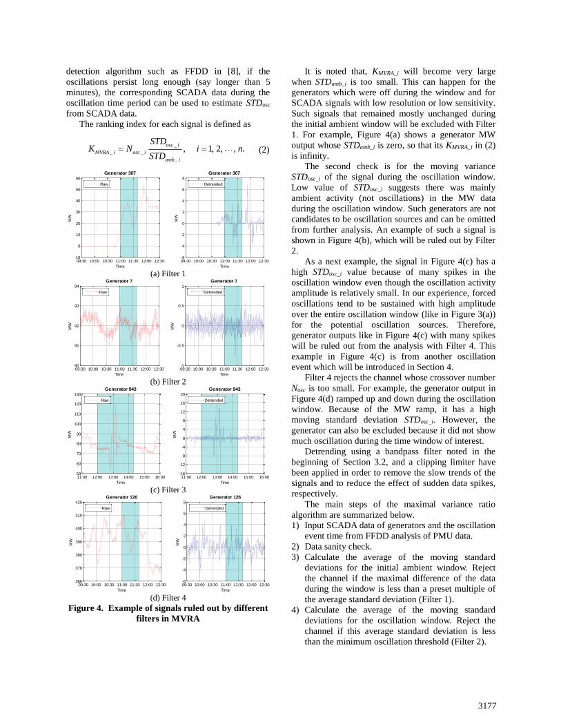
Figure 4. Example of signals ruled out by different

filters in MVRA

It is noted that, KMVRA_i will become very large

when STDamb_i is too small. This can happen for the

generators which were off during the window and for

SCADA signals with low resolution or low sensitivity.

Such signals that remained mostly unchanged during

the initial ambient window will be excluded with Filter

1. For example, Figure 4(a) shows a generator MW

output whose STDamb_i is zero, so that its KMVRA_i in (2)

is infinity.

The second check is for the moving variance

STDosc_i of the signal during the oscillation window.

Low value of STDosc_i suggests there was mainly

ambient activity (not oscillations) in the MW data

during the oscillation window. Such generators are not

candidates to be oscillation sources and can be omitted

from further analysis. An example of such a signal is

shown in Figure 4(b), which will be ruled out by Filter

2.

As a next example, the signal in Figure 4(c) has a

high STDosc_i value because of many spikes in the

oscillation window even though the oscillation activity

amplitude is relatively small. In our experience, forced

oscillations tend to be sustained with high amplitude

over the entire oscillation window (like in Figure 3(a))

for the potential oscillation sources. Therefore,

generator outputs like in Figure 4(c) with many spikes

will be ruled out from the analysis with Filter 4. This

example in Figure 4(c) is from another oscillation

event which will be introduced in Section 4.

Filter 4 rejects the channel whose crossover number

Nosc is too small. For example, the generator output in

Figure 4(d) ramped up and down during the oscillation

window. Because of the MW ramp, it has a high

moving standard deviation STDosc_i. However, the

generator can also be excluded because it did not show

much oscillation during the time window of interest.

Detrending using a bandpass filter noted in the

beginning of Section 3.2, and a clipping limiter have

been applied in order to remove the slow trends of the

signals and to reduce the effect of sudden data spikes,

respectively.

The main steps of the maximal variance ratio

algorithm are summarized below.

1) Input SCADA data of generators and the oscillation

event time from FFDD analysis of PMU data.

2) Data sanity check.

3) Calculate the average of the moving standard

deviations for the initial ambient window. Reject

the channel if the maximal difference of the data

during the window is less than a preset multiple of

the average standard deviation (Filter 1).

4) Calculate the average of the moving standard

deviations for the oscillation window. Reject the

channel if this average standard deviation is less

than the minimum oscillation threshold (Filter 2).

3177

5) Detrend using the bandpass filter.

6) Reject the channel if the number of spikes inside

the oscillation window is no less than the spike

count threshold (Filter 3).

7) Apply the clipping limiter for the oscillation

window.

8) Count the number of times the data values cross

their mean value within the oscillation window

Nosc_i.

9) Reject the channel if Nosc_i is less than a preset

factor of the number of samples inside the

oscillation window (Filter 4).

10) Recalculate the moving standard deviations over

both the initial ambient window and the oscillation

window for the filtered data, and compute the

average STDamb_i and STDosc_i for the two windows,

respectively.

11) Compute the ranking index KMVRA_i according to (2).

12) Apply step 2 to 11 for the rest of channels.

13) Select Top 3 channels based on the ranking index.

14) Inspect the MW outputs of the possible oscillation

sources for manual verification.

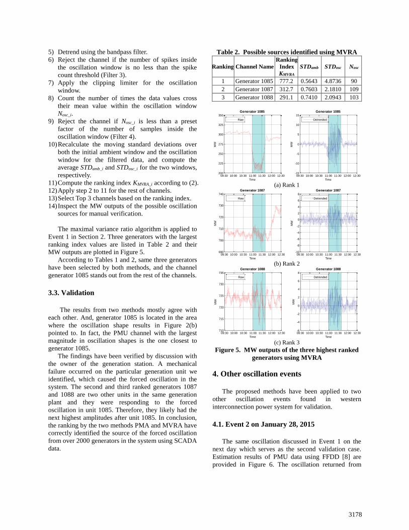
The maximal variance ratio algorithm is applied to

Event 1 in Section 2. Three generators with the largest

ranking index values are listed in Table 2 and their

MW outputs are plotted in Figure 5.

According to Tables 1 and 2, same three generators

have been selected by both methods, and the channel

generator 1085 stands out from the rest of the channels.

3.3. Validation

The results from two methods mostly agree with

each other. And, generator 1085 is located in the area

where the oscillation shape results in Figure 2(b)

pointed to. In fact, the PMU channel with the largest

magnitude in oscillation shapes is the one closest to

generator 1085.

The findings have been verified by discussion with

the owner of the generation station. A mechanical

failure occurred on the particular generation unit we

identified, which caused the forced oscillation in the

system. The second and third ranked generators 1087

and 1088 are two other units in the same generation

plant and they were responding to the forced

oscillation in unit 1085. Therefore, they likely had the

next highest amplitudes after unit 1085. In conclusion,

the ranking by the two methods PMA and MVRA have

correctly identified the source of the forced oscillation

from over 2000 generators in the system using SCADA

data.

Table 2. Possible sources identified using MVRA

Ranking Channel Name

Ranking

Index

KMVRA

STDamb STDosc Nosc

1 Generator 1085 777.2 0.5643 4.8736 90

2 Generator 1087 312.7 0.7603 2.1810 109

3 Generator 1088 291.1 0.7410 2.0943 103

Generator 1085

Time

MW

09:30 10:00 10:30 11:00 11:30 12:00 12:30200

225

250

275

300

325

350

Raw

Generator 1085

Time

MW

09:30 10:00 10:30 11:00 11:30 12:00 12:30-15

-10

-5

0

5

10

15

Detrended

(a) Rank 1 Generator 1087

Time

MW

09:30 10:00 10:30 11:00 11:30 12:00 12:30690

700

710

720

730

740

Raw

Generator 1087

Time

MW

09:30 10:00 10:30 11:00 11:30 12:00 12:30-10

-8

-6

-4

-2

0

2

4

6

8

Detrended

(b) Rank 2 Generator 1088

Time

MW

09:30 10:00 10:30 11:00 11:30 12:00 12:30710

715

720

725

730

735

Raw

Generator 1088

Time

MW

09:30 10:00 10:30 11:00 11:30 12:00 12:30-6

-4

-2

0

2

4

6

8

Detrended

(c) Rank 3


generators using MVRA

4. Other oscillation events

The proposed methods have been applied to two

other oscillation events found in western

interconnection power system for validation.

4.1. Event 2 on January 28, 2015

The same oscillation discussed in Event 1 on the

next day which serves as the second validation case.

Estimation results of PMU data using FFDD [8] are

provided in Figure 6. The oscillation returned from

3178

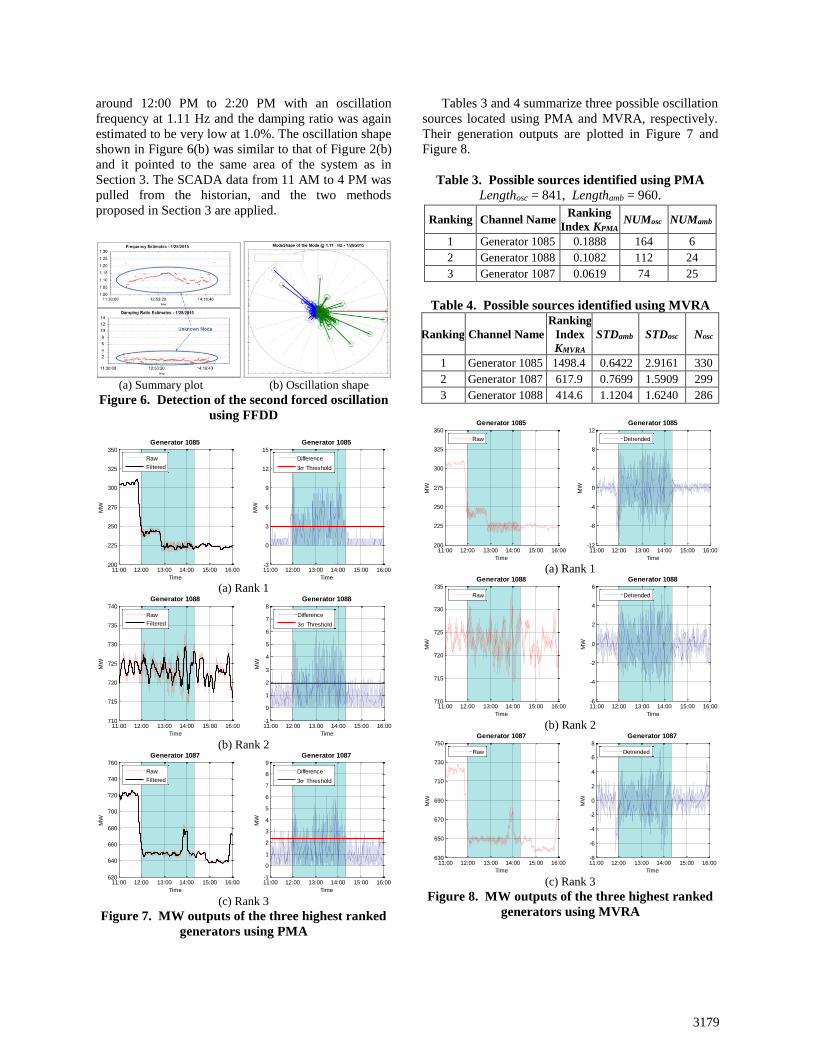
around 12:00 PM to 2:20 PM with an oscillation

frequency at 1.11 Hz and the damping ratio was again

estimated to be very low at 1.0%. The oscillation shape

shown in Figure 6(b) was similar to that of Figure 2(b)

and it pointed to the same area of the system as in

Section 3. The SCADA data from 11 AM to 4 PM was

pulled from the historian, and the two methods

proposed in Section 3 are applied.


Figure 6. Detection of the second forced oscillation

using FFDD

Generator 1085

Time

MW

11:00 12:00 13:00 14:00 15:00 16:00200

225

250

275

300

325

350

Raw

Filtered

Generator 1085

Time

MW

11:00 12:00 13:00 14:00 15:00 16:00-3

0

3

6

9

12

15

Difference

3 Threshold

(a) Rank 1

Generator 1088

Time

MW

11:00 12:00 13:00 14:00 15:00 16:00710

715

720

725

730

735

740

Raw

Filtered

Generator 1088

Time

MW

11:00 12:00 13:00 14:00 15:00 16:00-1

0

1

2

3

4

5

6

7

8

Difference

3 Threshold

(b) Rank 2

Generator 1087

Time

MW

11:00 12:00 13:00 14:00 15:00 16:00620

640

660

680

700

720

740

760

Raw

Filtered

Generator 1087

Time

MW

11:00 12:00 13:00 14:00 15:00 16:00-1

0

1

2

3

4

5

6

7

8

9

Difference

3 Threshold

(c) Rank 3



Tables 3 and 4 summarize three possible oscillation

sources located using PMA and MVRA, respectively.

Their generation outputs are plotted in Figure 7 and

Figure 8.





1 Generator 1085 0.1888 164 6

2 Generator 1088 0.1082 112 24

3 Generator 1087 0.0619 74 25



Ranking

Index

KMVRA

STDamb STDosc Nosc

1 Generator 1085 1498.4 0.6422 2.9161 330

2 Generator 1087 617.9 0.7699 1.5909 299

3 Generator 1088 414.6 1.1204 1.6240 286

Generator 1085

Time

MW

11:00 12:00 13:00 14:00 15:00 16:00200

225

250

275

300

325

350

Raw

Generator 1085

Time

MW

11:00 12:00 13:00 14:00 15:00 16:00-12

-8

-4

0

4

8

12

Detrended

(a) Rank 1

Generator 1088

Time

MW

11:00 12:00 13:00 14:00 15:00 16:00710

715

720

725

730

735

Raw

Generator 1088

Time

MW

11:00 12:00 13:00 14:00 15:00 16:00-6

-4

-2

0

2

4

6

Detrended

(b) Rank 2

Generator 1087

Time

MW

11:00 12:00 13:00 14:00 15:00 16:00630

650

670

690

710

730

750

Raw

Generator 1087

Time

MW

11:00 12:00 13:00 14:00 15:00 16:00-8

-6

-4

-2

0

2

4

6

8

Detrended

(c) Rank 3



3179

Like in the case of Event 1, generator 1085 is

ranked the most likely candidate to be the source of the

forced oscillation for Event 2 as well. Again, two other

units in the same plant, namely, generators 1087 and

1088 are ranked the next highest by both methods. As

stated earlier, a mechanical valve failure in generator

1085 did indeed cause the forced oscillation for this

event as well and the source of the oscillation being

generator 1085 was confirmed by the generation owner.

4.2. Event 3 on March 10, 2015

The third oscillation event was detected on March

10, 2015, which propagated through a major portion of

the western interconnection power system.

Figure 9 provides the estimation results of the

FFDD engine from [8]. It shows that an oscillation was

detected from around 11:02 AM to 11:07 AM. The

oscillation frequency was at 1.47 Hz and the damping

ratio was estimated to be very low as 0.34%, which

indicated that a possible forced oscillation had

occurred. In this event, since there was no PMU close

to the oscillation source, there were dozens of PMU

channels whose magnitudes were relatively large in the

oscillation shape results in Figure 9(b). The oscillation

can be clearly seen in the time plot of a line current

magnitude from a PMU shown in Figure 9(c).

Compared to the two previous oscillation events

discussed earlier in the paper, this case is more

challenging because the oscillations lasted only about 5

minutes. The 5 minute oscillation window consists of

only 30 SCADA data points at the 10 second sampling

rate.


(c) Time-plot of a line current magnitude from a PMU

Figure 9. Detection of the third forced oscillation

event using FFDD

To apply the two algorithms of Section 3, SCADA

data from 10 AM to 12 PM was extracted from the

historian and the ranking indices of Section 3 were

estimated. The three highest ranked possible oscillation

sources identified using PMA and MVRA are

summarized in Table 5 and Table 6, respectively. Their

SCADA generation outputs are shown in Figures 10

and 11.





1 Generator 1215 0.2903 9 0

2 Generator 2278 0.2186 7 5

3 Generator 945 0.1410 5 14



Ranking

Index

KMVRA

STDamb STDosc Nosc

1 Generator 1215 1031.1 0.1142 9.8159 12

2 Generator 2278 113.1 0.1397 1.5795 10

3 Generator 2280 56.3 0.7653 3.9141 11

Generator 1215

Time

MW

10:00 10:30 11:00 11:30 12:00-20

0

20

40

60

80

100

Raw

Filtered

Generator 1215

TimeM

W

10:00 10:30 11:00 11:30 12:00-5

0

5

10

15

20

25

30

35

Difference

3 Threshold

(a) Rank 1

Generator 2278

Time

MW

10:00 10:30 11:00 11:30 12:0026

27

28

29

30

31

32

33

Raw

Filtered

Generator 2278

Time

MW

10:00 10:30 11:00 11:30 12:00-1

0

1

2

3

4

Difference

3 Threshold

(b) Rank 2

Generator 945

Time

MW

10:00 10:30 11:00 11:30 12:00130

150

170

190

210

230

250

Raw

Filtered

Generator 945

Time

MW

10:00 10:30 11:00 11:30 12:00-1

0

1

2

3

4

Difference

3 Threshold

(c) Rank 3



3180

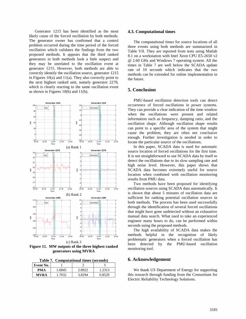
Generator 1215 has been identified as the most

likely cause of the forced oscillation by both methods.

The generator owner has confirmed that a control

problem occurred during the time period of the forced

oscillation which validates the findings from the two

proposed methods. It appears that the third ranked

generators in both methods look a little suspect and

they may be unrelated to the oscillation event at

generator 1215. However, both methods are able to

correctly identify the oscillation source, generator 1215

in Figures 10(a) and 11(a). They also correctly point to

the next highest ranked unit, namely generator 2278,

which is clearly reacting to the same oscillation event

as shown in Figures 10(b) and 11(b).

Generator 1215

Time

MW

10:00 10:30 11:00 11:30 12:00-20

0

20

40

60

80

100

Raw

Generator 1215

Time

MW

10:00 10:30 11:00 11:30 12:00-50

-40

-30

-20

-10

0

10

20

Detrended

(a) Rank 1

Generator 2278

Time

MW

10:00 10:30 11:00 11:30 12:0026

27

28

29

30

31

32

33

Raw

Generator 2278

Time

MW

10:00 10:30 11:00 11:30 12:00-4

-3

-2

-1

0

1

2

3

4

Detrended

(b) Rank 2

Generator 2280

Time

MW

10:00 10:30 11:00 11:30 12:00120

130

140

150

160

170

Raw

Generator 2280

Time

MW

10:00 10:30 11:00 11:30 12:00-8

-6

-4

-2

0

2

4

6

8

10

Detrended

(c) Rank 3



Table 7. Computational times (seconds)

Event No. 1 2 3

PMA 1.6845 2.8922 1.2313

MVRA 1.7032 3.8294 0.8529

4.3. Computational times

The computational times for source locations of all

three events using both methods are summarized in

Table VII. They are reported from tests using Matlab

8.1 on a workstation with Intel Xeon CPU E5-2650 v2

@ 2.60 GHz and Windows 7 operating system. All the

times in Table 7 are well below the SCADA update

rate of 10 seconds which indicates that the two

methods can be extended for online implementation in

the future.

5. Conclusion

PMU-based oscillation detection tools can detect

occurrence of forced oscillations in power systems.

They can provide a clear indication of the time window

when the oscillations were present and related

information such as frequency, damping ratio, and the

oscillation shape. Although oscillation shape results

can point to a specific area of the system that might

cause the problem, they are often not conclusive

enough. Further investigation is needed in order to

locate the particular source of the oscillations.

In this paper, SCADA data is used for automatic

source location of forced oscillations for the first time.

It is not straightforward to use SCADA data by itself to

detect the oscillations due to its slow sampling rate and

high noise level. However, this paper shows that

SCADA data becomes extremely useful for source

location when combined with oscillation monitoring

results from PMU data.

Two methods have been proposed for identifying

oscillation sources using SCADA data automatically. It

is shown that about 5 minutes of oscillation data are

sufficient for ranking potential oscillation sources in

both methods. The process has been used successfully

through the identification of several forced oscillations

that might have gone undetected without an exhaustive

manual data search. What used to take an experienced

engineer many hours to do, can be performed within

seconds using the proposed methods.

The high availability of SCADA data makes the

methods helpful in the recognition of likely

problematic generators when a forced oscillation has

been detected by the PMU-based oscillation

monitoring tool.

6. Acknowledgement

We thank US Department of Energy for supporting

this research through funding from the Consortium for

Electric Reliability Technology Solutions.

3181

7. References

[1] J. Van Ness, “Response of large power systems to cyclic

load variations, ” IEEE Trans. Power App. Syst.,

vol.PAS-85, no.7, pp. 723-727, Jul. 1966.

[2] C. D. Vournas, N. Krassas, and B. C. Papadias,

“Analysis of forced oscillations in a multimachine

power system, ” in Proc. Int. Conf. Contr., Edinburgh,

U.K., Mar. 1991, pp. 443-448.

[3] J. Ma, P. Zhang, H. Fu, B. Bo and Z. Dong,

“Application of Phasor Measurement Unit on Locating

Disturbance Source for Low-Frequency Oscillation,”

IEEE Trans. Smart Grid, vol.1, no.3, pp. 340-346, Dec.

2010.

[4] N. Zhou, “A cross-coherence method for detecting

oscillations, ” IEEE Trans. Power Syst., DOI:

10.1109/TPWRS.2015.2404804, to appear.

[5] J. Follum and J. W. Pierre, “Detection of periodic forced

oscillations in power systems,” IEEE Trans. Power

Syst., DOI: 10.1109/TPWRS.2015.2456919, to appear.

[6] S. A. Nezam Sarmadi and V. Venkatasubramanian,

“Inter-area resonance in power systems from forced

oscillations,” IEEE Trans. Power Syst., DOI:

10.1109/TPWRS.2015.2400133, to appear.

[7] K. Kim, et al., “Methods for calculating oscillations in

large power systems,” IEEE Trans. Power Syst., vol.

12, no. 4, pp. 1639–1648, Nov. 1997.

[8] H. Khalilinia, L. Zhang, and V. Venkatasubramanian,

“Fast frequency-domain decomposition for ambient

oscillation monitoring”, IEEE Trans. Power Del., vol.30,

no. 3, pp. 1631-1633, Jun. 2015.

3182

source location of forced oscillations using … location of forced oscillations using synchrophasor...

Documents