Note: This technical note is part of a series for bioluminescence tomography. You must first complete the steps in the previous bioluminescence tomography technical notes: Setup and Acquisition (4a) and Topography (4b) before proceeding.

1. Open DLIT 3D Reconstruction tab in Tool Palette.

2. Under the Analyze tab, choose the filters to be used for reconstruction. The filters correspond to the images acquired in your sequence in step one of this procedure.

Note: Living Image will automatically deselect a filter acquisition due to oversaturation or weak signal. For firefly luciferase 580, 600 and 620 nm are essential. Please repeat the acquisition if you do not have sufficient Signal (> 600 counts) at these wavelengths.

3. In the Properties tab, adjust the Tissue Properties to best represent the subject (mouse tissue or phantom) as well as the Source Spectrum (firefly, bacteria, etc.)

Note: If you used the Imaging Wizard for acquisition, these selections will use the input received through the Wizard automatically.

4. Once the filters and properties have been set, click the Start button under the Analyze tab to review the sequence to be used for reconstruction.

T E C H N I C A L N O T E

Pre-clinical in vivo imaging

Source Reconstruction and Analysis

Technical Note 4c

2

5. The Data Preview tab will be displayed in which you can adjust and threshold your data. Thresholds typically default below 5% so most of the signal is included in the analysis. Occasionally a small source will be excluded, you can adjust the threshold down slightly to include more signal in the analysis by checking Select All and Data Adjustment at the bottom of the window. As a general rule, do not decrease thresholds below 0.5% as DLIT artifacts may reconstruct. In most cases, default settings chosen by the software will suffice.

You can also adjust the threshold for individual images by double clicking on the image you wish to adjust. Within this window is also a masking tool that will allow you to mask in a region of the mouse for consideration and exclude other areas. See the User Guide for more information on using this tool.

6. Once the sequence has been approved and the Data Adjustment (if any) has been set, click the Reconstruct button to create the bioluminescent 3D source.

7. When the reconstruction has finished, the Results tab will display statistical data about the calculation. Check for an accurate reconstruction by opening the Photon Density Map and comparing the Measured light diffusion pattern vs. the Simulated light diffusion pattern. The % error between these two maps is illustrated on the bottom row. If the bottom row has a near-zero % difference between Measured and Simulated maps (indicated with a green color), the reconstruction was successful and the image may be used for quantification and spatial measurements.

8. Name and Save your DLIT reconstruction with the Save button on the bottom right corner of the Results tab.

% Error between Measured and Simulated diffusion patterns per image. Green means “Go”.

Masked region

3

9. Once the reconstruction has been saved, the 3D Optical Tools section of the Tool Palette will provide access to three sections of the reconstruction: Surface, Source and Registration. By default, the Subject Surface, or topographic map, will be turned on to allow 3D orientation of your source inside the subject. This Subject Surface can be altered for color, opacity and geometrical rendering using the options in the Surface tab.

Additionally, you may select to visualize the 2D light diffusion pattern, either the Simulated or Measured, for each wavelength used in the analysis by clicking the Display Photon Density Map box.

10. The Source tab contains all the tools necessary to adjust visualization of the reconstructed bioluminescent sources. Sources consist of multiple Voxels (3D pixels) representing relative intensity at that spatial location within the subject.

Two visualization choices are available: Display Source Surface and Display Voxels. Choosing Display Source Surface displays the isosurface of the reconstructed source volume. Users can adjust the color and geometric rendering of the bioluminescent source. It is useful for screenshots, movies, and other visualizations. Quantitative signal intensity and depth measurements are not possible when this option is chosen.

For quantification of your source, you must select Display Voxels. The displayed source represents a 3D diffusion pattern and it can be selected using the Voxel Selection Tool and at-source measurements can be recorded (see Step 12 – Page 4).

You can adjust the look of the reconstructed source with the Color Table drop down menu and the Color Scale slider to adjust minimum visualized values. Avoid adjusting the size of your source using the Threshold slider as this removes voxels from consideration when measuring for quantitative output.

11. The Registration tab of 3D Optical Tools allows for an overlay of your Surface/Source reconstruction with a generic Mouse Organ Atlas.

Find the appropriate sex and orientation via the dropdown menu and select one of the three Registration Tools: Manual, Linear Automatic and Non-linear Automatic.

Linear and Non-linear automatic use the Surface reconstruction to perform a best fit for the Organ Atlas.

Manual co-registration provides panning, shrink/grow and rotational position options to overlay the Organ Atlas to the Surface shape. When Manual is selected, use the ‘Tab’ button to cycle through the 3 tool sets. Once the co-registration is set, organs may be removed or selected to appear in the 3D image along with the bioluminescent source by checking/unchecking the box next to the organ name. The colors of the organs cannot be changed but the transparency of the organs can be adjusted with the provided Opacity slider bar.

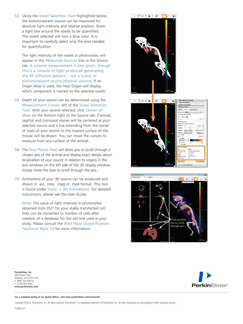
12. Using the Voxel Selection Tool highlighted below, the bioluminescent source can be measured for absolute light intensity and relative position. Draw a tight box around the voxels to be quantified. The voxels selected will turn a blue color. It is important to carefully select only the area needed for quantification.

The light intensity of the voxels in photons/sec will appear in the Measured Sources box in the Source tab. A volume measurement is also given, though this is a volume of light produced generating the 3D diffusion pattern – not a tumor or bioluminescent source physical volume. If an Organ Atlas is used, the Host Organ will display which component is nearest to the selected voxels.

13. Depth of your source can be determined using the Measurement Cursor, left of the Voxel Selection Tool. With your source selected, click Center of Mass on the bottom right of the Source tab. Coronal, sagittal and transaxial planes will be centered at your selected source and a line extending from the center of mass of your source to the nearest surface of the mouse will be drawn. You can move the cursors to measure from any surface of the animal.

14. The Slice Planes Tool will allow you to scroll through a chosen axis of the animal and display exact details about localization of your source in relation to organs in the axis windows on the left side of the 3D display window. Simply move the bars to scroll through the axis.

15. Animations of your 3D source can be produced and shown in .avi, .mov, .mpg or .mp4 format. This tool is found under Tools -> 3D Animations. For detailed instructions, please see the User Guide.

Note: The value of light intensity in photons/sec obtained from DLIT for your stably transfected cell lines can be converted to number of cells after creation of a database for the cell line used in your study. Please consult the Well Plate Quantification Technical Note 15 for more information.

For a complete listing of our global offices, visit www.perkinelmer.com/ContactUs

Copyright ©2012, PerkinElmer, Inc. All rights reserved. PerkinElmer® is a registered trademark of PerkinElmer, Inc. All other trademarks are the property of their respective owners. 010583_01

PerkinElmer, Inc. 940 Winter Street Waltham, MA 02451 USA P: (800) 762-4000 or (+1) 203-925-4602www.perkinelmer.com

Click and slide bars to scroll through axes.