southern riverine plains groundwater model calibration report · a.m. goode and b.g. barnett...

A.M. Goode and B.G. Barnett

September 2008

Southern Riverine Plains Groundwater Model Calibration ReportA report to the Australian Government from the CSIRO Murray-Darling Basin Sustainable Yields Project

Murray-Darling Basin Sustainable Yields Project acknowledgments

The Murray-Darling Basin Sustainable Yields project is being undertaken by CSIRO under the Australian Government's Raising National

Water Standards Program, administered by the National Water Commission. Important aspects of the work were undertaken by Sinclair

Knight Merz; Resource & Environmental Management Pty Ltd; Department of Water and Energy (New South Wales); Department of

Natural Resources and Water (Queensland); Murray-Darling Basin Commission; Department of Water, Land and Biodiversity

Conservation (South Australia); Bureau of Rural Sciences; Salient Solutions Australia Pty Ltd; eWater Cooperative Research Centre;

University of Melbourne; Webb, McKeown and Associates Pty Ltd; and several individual sub-contractors.

Murray-Darling Basin Sustainable Yields Project disclaimers

Derived from or contains data and/or software provided by the Organisations. The Organisations give no warranty in relation to the data

and/or software they provided (including accuracy, reliability, completeness, currency or suitability) and accept no liability (including

without limitation, liability in negligence) for any loss, damage or costs (including consequential damage) relating to any use or reliance

on that data or software including any material derived from that data and software. Data must not be used for direct marketing or be

used in breach of the privacy laws. Organisations include: Department of Water, Land and Biodiversity Conservation (South Australia),

Department of Sustainability and Environment (Victoria), Department of Water and Energy (New South Wales), Department of Natural

Resources and Water (Queensland), Murray-Darling Basin Commission.

CSIRO advises that the information contained in this publication comprises general statements based on scientific research. The reader

is advised and needs to be aware that such information may be incomplete or unable to be used in any specific situation. No reliance or

actions must therefore be made on that information without seeking prior expert professional, scientific and technical advice. To the

extent permitted by law, CSIRO (including its employees and consultants) excludes all liability to any person for any consequences,

including but not limited to all losses, damages, costs, expenses and any other compensation, arising directly or indirectly from using

this publication (in part or in whole) and any information or material contained in it. Data is assumed to be correct as received from the

Organisations.

Citation

Goode AM and Barnett BG (2008) Southern Riverine Plains Groundwater Model Calibration Report. A report to the Australian

Government from the CSIRO Murray-Darling Basin Sustainable Yields Project. CSIRO, Australia. 138pp.

Publication Details

Published by CSIRO © 2008 all rights reserved. This work is copyright. Apart from any use as permitted under the Copyright Act 1968,

no part may be reproduced by any process without prior written permission from CSIRO.

ISSN 1835-095X

Preface

This is a report to the Australian Government from CSIRO. It is an output of the Murray-Darling Basin Sustainable Yields

Project which assessed current and potential future water availability in 18 regions across the Murray-Darling Basin

(MDB) considering climate change and other risks to water resources. The project was commissioned following the

Murray-Darling Basin Water Summit convened by the Prime Minister of Australia in November 2006 to report

progressively during the latter half of 2007. The reports for each of the 18 regions and for the entire MDB are supported

by a series of technical reports detailing the modelling and assessment methods used in the project. This report is one of

the supporting technical reports of the project. Project reports can be accessed at http://www.csiro.au/mdbsy.

Project findings are expected to inform the establishment of a new sustainable diversion limit for surface and

groundwater in the MDB – one of the responsibilities of a new Murray-Darling Basin Authority in formulating a new

Murray-Darling Basin Plan, as required under the Commonwealth Water Act 2007. These reforms are a component of

the Australian Government’s new national water plan ‘Water for our Future’. Amongst other objectives, the national water

plan seeks to (i) address over-allocation in the MDB, helping to put it back on a sustainable track, significantly improving

the health of rivers and wetlands of the MDB and bringing substantial benefits to irrigators and the community; and (ii)

facilitate the modernisation of Australian irrigation, helping to put it on a more sustainable footing against the background

of declining water resources.

Executive summary

Background The Southern Riverine groundwater model has been developed for the Murray-Darling Basin Sustainable Yields Project.

Groundwater extraction across the Southern Riverine Plains of the Murray-Darling Basin (Figure A1 and Figure A2) plus

the neighbouring Murrumbidgee represents about 40% of the groundwater extraction within the Murray-Darling Basin.

While models existed for parts of this area, the nature of the groundwater system means that it is no longer appropriate

for these areas to be modelled independently. The area contains two significant environmental assets within the Living

Murray (Barmah-Millewa and Gunbower-Pericoota-Koontra), which may be dependent on groundwater. There is also

sufficient field evidence to suggest that extraction in the plain will have an impact on the streams in the region, including

the River Murray.

The Southern Riverine Plains is an area which has seen development of the groundwater resource since the early 1980s,

with extractions peaking in 2002/03 at slightly over 400 GL (currently averaging approximately 250 GL/year).The

development in the groundwater resource has seen it become an increasingly important component of water resource

management in the Murray-Darling Basin.

The groundwater model, described in this report, is designed to meet the objectives of the Murray-Darling Basin

Sustainable Yields Project. It is not the aim of this model to be able to determine the extraction limit of the area or any

sub-region thereof. However, the model is designed to assess the relative impacts of various climate scenarios and

groundwater pumping on the state of the groundwater resources.

The Southern Riverine groundwater model combines a number of existing groundwater models within the area: the New

South Wales Lower Murray model (DLWC, 2001), the Katunga WSPA groundwater model and the Campaspe WSPA

groundwater model (the Campaspe model was developed in an earlier phase of this project and later superceded by this

model). By combining these models, we attempt to minimise the controlling influence of artificial model boundary

conditions and provide an enhanced representation of intermediate and regional scale interference patterns. As

previously stated this also provides an ability to advance water accounting capabilities across state and management

area boundaries.

Model description The groundwater model was constructed within the Visual Modflow modelling framework. It spans approximately 290 km

from east to west and 250 km from north to south with a 1 km2 grid cell resolution. It incorporates the major surface

drainage features of the Murray River, Edward River, Wakool River, Neimur Creek, Loddon River, Campaspe River and

© CSIRO 2008 Southern Riverine Plains Groundwater Model Calibration Report

the Goulburn and Broken rivers. Geologically the model is divided into four layers: Upper Shepparton, Lower Shepparton,

Calivil Formation and Renmark Group layers. The Calivil and Renmark together form the major aquifer, which hold a

significant groundwater resource. These two layers are commonly referred to as the Deep Lead in Victoria, but take the

form of a broad sheet of material in New South Wales.

The model covers nine individual groundwater management units and four regions, as defined by this project. It also

includes possible groundwater-dependent ecosystems such as Gunbower Forest, Koondrook-Perricoota Forest, and the

Barmah Forest.

The groundwater model calibration was completed at an adequate level that meets the requirements of a moderate

complexity regional scale groundwater model as defined in Murray-Darling Basin Commission Groundwater Flow

Modelling Guidelines (Middlemis, 2000).

Modelling results and key messages Key messages identified from the modelling are discussed below.

Water accounting across groundwater management unit (GMU) boundaries – The results from the groundwater

modelling highlight the significant levels of interaction that occur between neighbouring GMUs and regions. In particular it

was found that there are significant fluxes of groundwater beneath the Murray River in the Deep Lead aquifers. For

example, there are high levels of groundwater extractions in the Lower Murray GWMA in New South Wales (~80

GL/year). In the model approximately 50% of this volume pumped (40 GL/year) is drawn from groundwater resources to

the north (from the Murrumbidgee Catchment) and from south of the Murray River.

Similarly pumping in the Katunga and Shepparton WSPAs draws large volumes of water from groundwater resources to

the south and causes water to flow out of the Kialla and the Mid-Goulburn GMAs. As a result, the predictive scenarios

include a net flux of groundwater out of the Kialla and Mid-Goulburn GMAs. This occurs in spite of increased extractions

from within these GMAs. A model constructed for the Kialla GMA or Mid-Goulburn GMA in isolation (i.e. not including the

neighbouring WSPAs) would have presented the opposite result. Individual isolated models predict net groundwater

influxes in response to increasing groundwater extraction. This finding highlights the importance of modelling the entire

aquifer as a whole and not splitting it up into a number of smaller groundwater models based on groundwater

management regions. It further highlights the fact that neighbouring groundwater models constructed in the same aquifer

will lead to significant accounting errors associated with groundwater fluxes across lateral model boundaries.

Surface–groundwater interactions – Current (2004/05) rates of groundwater extraction in the Southern Riverine model

are approximately 250 GL/year. Compared to without-development conditions, it was found that 42% (103 GL/year) of

the current groundwater pumping is sourced from surface waters (i.e. from reduced flow in rivers) within the model area.

However, due to limitations in modelling the without-development conditions it is believed that this figure is likely to be as

high as 60% (150 GL/year). This latter figure is supported by modelling results of future conditions (scenarios C and D)

where pumping is increased by a further 50 GL/year to ~300 GL/year. Here it was found that 58% of the additional

volume extracted was sourced from loss of river flow. The remainder of the volume extracted was obtained from

captured or reduced groundwater evapotranspiration, 37%, with 5% sourced from changes in lateral flow across model

boundaries. This small volume sourced from changes in fluxes across model boundaries suggests that the model is

correctly accounting for the regional scale impacts of groundwater pumping. These issues are discussed in detail in

Section 6.2.

The time lag associated with the impacts of groundwater pumping on streamflows varies on a scale from years to several

decades, depending on the depth and location of extraction wells. Under Scenario A the full impacts of all groundwater

extractions are observed within 25 years.

Groundwater evapotranspiration (ET) and groundwater-dependent ecosystems (GDEs) – The importance of

groundwater ET was first highlighted during the calibration process where it was discovered that groundwater ET from

forested areas, such as the Gunbower Forest, had a significant influence on the groundwater levels. From the predictive

scenario modelling results ET proved to be the groundwater discharge process that is most sensitive to climate change.

Under the dry scenarios, decreases in rainfall recharge were largely matched by decreases in groundwater ET. This is

mostly realised by losses in water availability to GDEs. In practical terms, this suggests that unless water allocations are

reduced in accordance with the reduced rainfall recharge it is possible that GDEs are likely to suffer from reduced water

availability as a result of climate change.

Southern Riverine Plains Groundwater Model Calibration Report © CSIRO 2008

All of the modelled scenarios reached dynamic equilibrium within the 222-year modelling period (111 years of warm-up

and 111 years of scenario). This suggests that current rates of groundwater extractions will eventually achieve a balance

in groundwater inflows and outflows. However, current groundwater use has already and will continue to cause

significant drawdown in groundwater levels across the Riverine Plains. As a result continued groundwater extraction at

current rates will draw heavily on surface water resources and is possibly already impacting on GDEs.

Figure A1. Map of the Southern Riverine Plains Model within the Murray-Darling Basin

Figure A2. Detailed map of the Southern Riverine Plains Model


Table of Contents

1 Introduction............................................................................................................................... 1

2 Hydrogeological conceptualisation...................................................................................... 2 2.1 Modelling area and physiography .................................................................................................................................2 2.2 Geological setting.........................................................................................................................................................3 2.3 Regions and groundwater management units...............................................................................................................5

2.3.1 Murray (NSW GWMA 016, Katunga WSPA)...................................................................................................6 2.3.2 Loddon-Avoca (Mid-Loddon GMA) .................................................................................................................7 2.3.3 Campaspe (Campaspe Deep Lead WSPA, Ellesmere GMA) .........................................................................7 2.3.4 Goulburn-Broken (Mid-Goulburn GMA, Kialla GMA, Goorambat GMA) ..........................................................8 2.3.5 Shepparton WSPA .........................................................................................................................................8

3 Model development .............................................................................................................. 10 3.1 Model domain.............................................................................................................................................................10

3.1.1 Study area....................................................................................................................................................10 3.1.2 Coordinate system .......................................................................................................................................11 3.1.3 Model layering..............................................................................................................................................11

3.2 Model input data.........................................................................................................................................................15 3.2.1 Storage parameters......................................................................................................................................15 3.2.2 Hydrogeological conductivity values .............................................................................................................15 3.2.3 Rivers and drains .........................................................................................................................................20 3.2.4 Recharge (dryland and irrigation) .................................................................................................................21 3.2.5 Evapotranspiration .......................................................................................................................................26 3.2.6 Boundary conditions.....................................................................................................................................27

4 Model calibration................................................................................................................... 29 4.1 Calibration method .....................................................................................................................................................29

4.1.1 Groundwater extraction ................................................................................................................................29 4.1.2 Calibration model observation bores ............................................................................................................34

4.2 Calibration model results ............................................................................................................................................36 4.3 Summary of hydrographs by region............................................................................................................................36

4.3.1 Murray..........................................................................................................................................................36 4.3.2 Loddon-Avoca..............................................................................................................................................40 4.3.3 Campaspe....................................................................................................................................................41 4.3.4 Goulburn-Broken..........................................................................................................................................43

4.4 Potentiometric surface maps ......................................................................................................................................45 4.4.1 Shepparton Formation..................................................................................................................................46 4.4.2 Deep Lead ...................................................................................................................................................47

4.5 Calibration statistics ...................................................................................................................................................48 4.6 Calibration model water balance.................................................................................................................................48

4.6.1 Overview......................................................................................................................................................48 4.6.2 Surface–groundwater interaction..................................................................................................................50

4.7 Groundwater management unit water balances..........................................................................................................52 4.7.1 Lower Murray (NSW GWMA 016).................................................................................................................53 4.7.2 Mid-Loddon ..................................................................................................................................................53 4.7.3 Campaspe Deep Lead .................................................................................................................................54 4.7.4 Ellesmere.....................................................................................................................................................54 4.7.5 Katunga........................................................................................................................................................54 4.7.6 Kialla ............................................................................................................................................................55 4.7.7 Mid-Goulburn ...............................................................................................................................................55 4.7.8 Goorambat ...................................................................................................................................................55 4.7.9 Shepparton ..................................................................................................................................................56

5 Scenario modelling methodology ....................................................................................... 57 5.1 Model scenarios .........................................................................................................................................................57 5.2 Alterations to the calibration model.............................................................................................................................57 5.3 Scenario model inputs ................................................................................................................................................57

5.3.1 Recharge .....................................................................................................................................................57 5.3.2 Rivers and drains .........................................................................................................................................58 5.3.3 Extractions ...................................................................................................................................................58 5.3.4 Evapotranspiration .......................................................................................................................................58 5.3.5 Boundary conditions.....................................................................................................................................58

5.4 Key indicator bores.....................................................................................................................................................59 5.5 Integration into the whole-of-MDB modelling framework .............................................................................................60 5.6 Scenario reporting structure .......................................................................................................................................62

6 Scenario modelling results .................................................................................................... 63 6.1 Groundwater levels ....................................................................................................................................................63 6.2 Surface–groundwater interactions ..............................................................................................................................65 6.3 Groundwater balance .................................................................................................................................................66

6.3.1 Overview......................................................................................................................................................66


6.3.2 Groundwater extractions ..............................................................................................................................68 6.4 Groundwater indicators ..............................................................................................................................................69

7 Results by groundwater management unit......................................................................... 71 7.1 Campaspe Deep Lead WSPA ....................................................................................................................................71

7.1.1 Groundwater resource condition indicators...................................................................................................73 7.2 Ellesmere GMA ..........................................................................................................................................................73

7.2.1 Groundwater resource condition indicators...................................................................................................74 7.3 Goorambat GMA ........................................................................................................................................................75

7.3.1 Groundwater resource condition indicators...................................................................................................76 7.4 Katunga WSPA ..........................................................................................................................................................76

7.4.1 Groundwater resource condition indicators...................................................................................................78 7.5 Kialla GMA .................................................................................................................................................................78

7.5.1 Groundwater resource condition indicators...................................................................................................80 7.6 Lower Murray (NSW GWMA 016)...............................................................................................................................80

7.6.1 Groundwater resource condition indicators...................................................................................................83 7.7 Mid-Goulburn GMA ....................................................................................................................................................83

7.7.1 Groundwater resource condition indicators...................................................................................................85 7.8 Mid-Loddon GMA .......................................................................................................................................................85

7.8.1 Groundwater resource condition indicators...................................................................................................87 7.9 Shepparton WSPA .....................................................................................................................................................87

7.9.1 Groundwater resource condition indicators...................................................................................................89

8 Results by region .................................................................................................................... 90 8.1 Campaspe..................................................................................................................................................................90 8.2 Goulburn-Broken........................................................................................................................................................91 8.3 Loddon-Avoca ............................................................................................................................................................93 8.4 Murray........................................................................................................................................................................95

9 Discussion of results................................................................................................................ 97

10 Modelling limitations and recommendations..................................................................... 99

11 References ............................................................................................................................ 101

12 Appendix A – River gauges ................................................................................................ 102

13 Appendix B – Calibration model observation bores........................................................ 104

14 Appendix C – Calibration model hydrographs ................................................................ 107 14.1 New South Wales.....................................................................................................................................................107 14.2 Gunbower Forest......................................................................................................................................................111 14.3 Loddon .....................................................................................................................................................................113 14.4 Campaspe................................................................................................................................................................116 14.5 Katunga....................................................................................................................................................................120 14.6 Goulburn-Broken......................................................................................................................................................124

15 Appendix D – Natural flows scenario results..................................................................... 131 15.1 Introduction ..............................................................................................................................................................131 15.2 Model results............................................................................................................................................................131 15.3 GMU water balances................................................................................................................................................133 15.4 Regional water balances ..........................................................................................................................................136


Tables

Table 3-1. Spatial parameters of the model coordinate system ......................................................................................................11 Table 3-2. Storage parameters defined in the model......................................................................................................................15 Table 3-3. Southern Riverine modelled recharge zones.................................................................................................................23 Table 4-1. Calibration model performance criteria (after Middlemis, 2000).....................................................................................29 Table 4-2. Estimated groundwater usage in New South Wales (supplied by the New South Wales Department of Natural Resources) ....................................................................................................................................................................................30 Table 4-3. Groundwater usage estimates in Victorian groundwater management units..................................................................32 Table 4-4. Groundwater usage estimates for Victorian unincorporated areas (grouped by catchment)...........................................32 Table 4-5. Calibration model statistics ...........................................................................................................................................48 Table 4-6. Average annual groundwater inflows and outflows for each groundwater management unit within the model area (January 1990 to December 2005).................................................................................................................................................52 Table 5-1. Summary of the scenario models..................................................................................................................................57 Table 5-2. Groundwater extraction data for the Southern Riverine scenario models ......................................................................58 Table 5-3. Groundwater monitoring sites used in the scenario modelling .......................................................................................59 Table 6-1. Median groundwater changes (m) across the Southern Riverine model under scenarios A, B, C and D........................63 Table 6-2. Impacts of groundwater pumping on net river losses.....................................................................................................66 Table 6-3. Modelled average annual groundwater balance under scenarios A, B, C and D and under the without-development scenario (second 111 years)..........................................................................................................................................................67 Table 6-4. Southern Riverine recharge compared to pumping under all scenarios.........................................................................69 Table 6-5. Definition of groundwater indicators ..............................................................................................................................69 Table 6-6. Groundwater indicators under scenarios A, B, C and D.................................................................................................70 Table 7-1. Groundwater balance for the Campaspe Deep Lead WSPA .........................................................................................71 Table 7-2. Median groundwater changes (m) in the Campaspe Deep Lead WSPA under scenarios A, B, C and D .......................73 Table 7-3. Groundwater indicators under scenarios A, B, C and D.................................................................................................73 Table 7-4. Groundwater balance for the Ellesmere GMA ...............................................................................................................73 Table 7-5. Median groundwater changes (m) in the Ellesmere GMA under scenarios A, B, C and D .............................................74 Table 7-6. Groundwater indicators under scenarios A, B, C and D.................................................................................................74 Table 7-7. Groundwater balance for the Goorambat GMA .............................................................................................................75 Table 7-8. Median groundwater changes (m) in the Goorambat GMU under scenarios A, B, C and D ...........................................76 Table 7-9. Groundwater indicators under scenarios A, B, C and D.................................................................................................76 Table 7-10. Groundwater balance for the Katunga WSPA .............................................................................................................76 Table 7-11. Median groundwater changes (m) in the Katunga WSPA under scenarios A, B, C and D............................................78 Table 7-12. Groundwater indicators under scenarios A, B, C and D...............................................................................................78 Table 7-13. Groundwater balance for the Kialla GMA ....................................................................................................................79 Table 7-14. Median groundwater changes (m) in the Kialla GMA under scenarios A, B, C and D ..................................................80 Table 7-15. Groundwater indicators under scenarios A, B, C and D...............................................................................................80 Table 7-16. Groundwater balance for the Lower Murray GWMA 016 – Calivil Formation and Renmark Group ..............................81 Table 7-17. Groundwater balance for the Lower Murray GWMA 016 – Shepparton Formation ......................................................81 Table 7-18. Median groundwater changes (m) in the Lower Murray groundwater management unit for baseline, recent and future scenarios .......................................................................................................................................................................................83 Table 7-19. Groundwater indicators for baseline, recent and future scenarios ...............................................................................83 Table 7-20. Groundwater balance for the Mid-Goulburn GMA........................................................................................................84 Table 7-21. Median groundwater changes (m) in the Mid-Goulburn GMA under scenarios A, B, C and D......................................85 Table 7-22. Groundwater indicators under scenarios A, B, C and D...............................................................................................85 Table 7-23. Groundwater balance for the Mid-Loddon GMA ..........................................................................................................86 Table 7-24. Median groundwater changes (m) in the Mid-Loddon GMU under scenarios A, B, C and D ........................................87 Table 7-25. Groundwater indicators under scenarios A, B, C and D...............................................................................................87 Table 7-26. Groundwater balance for the Shepparton WSPA ........................................................................................................88 Table 7-27. Median groundwater changes (m) in the Shepparton WSPA under scenarios A, B, C and D ......................................89 Table 7-28. Groundwater indicators under scenarios A, B, C and D...............................................................................................89 Table 8-1. Groundwater balance for the Campaspe region ............................................................................................................90 Table 8-2. Comparison of the without-development scenario and Scenario A in the Campaspe region..........................................91 Table 8-3. Groundwater balance for the Goulburn-Broken region ..................................................................................................92 Table 8-4. Comparison of the without-development scenario and Scenario A in the Goulburn-Broken region ................................93 Table 8-5. Groundwater balance for the Loddon-Avoca region ......................................................................................................93 Table 8-6. Comparison of the without-development scenario and Scenario A in the Goulburn-Broken region ................................94 Table 8-7. Groundwater balance for the Murray region ..................................................................................................................95


Table 8-8. Comparison of the without-development scenario and Scenario A in the Murray region................................................96 Table 15-1. Groundwater balance results under the natural flows scenario..................................................................................132 Table 15-2. Groundwater balance results under the natural flows scenario: Campaspe Deep Lead WSPA .................................133 Table 15-3. Groundwater balance results under the natural flows scenario: Ellesmere GMA .......................................................134 Table 15-4. Groundwater balance results under the natural flows scenario: Goorambat GMA .....................................................134 Table 15-5. Groundwater balance results under the natural flows scenario: Katunga WSPA .......................................................134 Table 15-6. Groundwater balance results under the natural flows scenario: Kialla GMA ..............................................................135 Table 15-7. Groundwater balance results under the natural flows scenario: Mid-Loddon GMA ....................................................135 Table 15-8. Groundwater balance results under the natural flows scenario: Lower Murray NSW GWMA 016 – Deep Lead.........135 Table 15-9. Groundwater balance results under the natural flows scenario: Lower Murray NSW GWMA 016 – Shepparton Formation ....................................................................................................................................................................................136 Table 15-10. Groundwater balance results under the natural flows scenario: Shepparton WSPA ................................................136 Table 15-11. Groundwater balance results under the natural flows scenario: Campaspe region ..................................................137 Table 15-12. Groundwater balance results under the natural flows scenario: Goulburn-Broken region ........................................137 Table 15-13. Groundwater balance results under the natural flows scenario: Loddon region .......................................................138 Table 15-14. Groundwater balance results under the natural flows scenario: Murray region ........................................................138

Figures

Figure 2-1. Major towns and rivers superimposed over satellite imagery of the model area .............................................................3 Figure 2-2. Southern Riverine model domain looking toward the Great Dividing Range in the south-east ........................................3 Figure 2-3. Regions within the Southern Riverine groundwater model .............................................................................................5 Figure 2-4. Groundwater management units within the Southern Riverine groundwater model ........................................................6 Figure 3-1. Southern Riverine model grid and coordinates in Lambert Conical Conformance projection ........................................10 Figure 3-2. Southern Riverine model domain including groundwater management areas and inactivated areas ............................11 Figure 3-3. East–west cross-section of the Southern Riverine model highlighting the hydrogeological layering structure of the model (vertically exaggerated by 300 times) ..................................................................................................................................12 Figure 3-4. Thickness of the Upper Shepparton Aquifer.................................................................................................................12 Figure 3-5. Thickness of the Lower Shepparton Aquifer.................................................................................................................13 Figure 3-6. Thickness of the Calivil Formation Aquifer ...................................................................................................................13 Figure 3-7. Thickness of the Renmark Group Aquifer ....................................................................................................................14 Figure 3-8. Hydraulic conductivity values in Layer 1 (Upper Shepparton Formation)......................................................................16 Figure 3-9. Hydraulic conductivity values in Layer 2 (Lower Shepparton).......................................................................................17 Figure 3-10. Hydraulic conductivity values in Layer 3 (Calivil Formation) .......................................................................................18 Figure 3-11. Hydraulic conductivity values in Layer 4 (Renmark Group) ........................................................................................19 Figure 3-12. Rivers and drains included in the Southern Riverine model........................................................................................20 Figure 3-13. All natural surface water features within the Southern Riverine model domain...........................................................21 Figure 3-14. Rainfall districts as defined by the Bureau of Meteorology (2006) ..............................................................................24 Figure 3-15. Satellite imagery highlighting irrigation areas incorporated into the Southern Riverine model.....................................24 Figure 3-16. Rainfall sites (1 to 20) input into the Waves Model to deduce dryland recharge variability across the model..............25 Figure 3-17. Southern Riverine model recharge zones ..................................................................................................................26 Figure 3-18. Groundwater evapotranspiration rates set across the Southern Riverine model.........................................................27 Figure 3-19. General head boundaries...........................................................................................................................................28 Figure 4-1. Estimated volumes of groundwater extractions in New South Wales ...........................................................................30 Figure 4-2. Distribution of groundwater pumping throughout a calendar year.................................................................................31 Figure 4-3. Estimated groundwater usage in the Victorian groundwater management units and unincorporated areas ..................33 Figure 4-4. Groundwater extraction wells included in the Southern Riverine model........................................................................33 Figure 4-5. Observation bores screening the Upper Shepparton....................................................................................................34 Figure 4-6. Observation bores screening the Lower Shepparton....................................................................................................35 Figure 4-7. Observation bores screening the Calivil Formation ......................................................................................................35 Figure 4-8. Observation bores screening the Renmark Group .......................................................................................................36 Figure 4-9. Example hydrographs from the Murray region near Deniliquin (note: this is not a nested site) .....................................37 Figure 4-10. Example hydrographs from the Murray region in the east between Corowa and Jerilderie .........................................38 Figure 4-11. Example hydrographs from the Murray region in the south near Echuca....................................................................38 Figure 4-12. Example hydrographs from the Murray region in Gunbower Forest............................................................................39 Figure 4-13. Example hydrographs from the north of the Loddon catchment in the Murray region .................................................39 Figure 4-14. Example hydrographs from the north-east of the Loddon catchment in the Murray region..........................................40 Figure 4-15. Example hydrographs from the Katunga WSPA within the Murray region ..................................................................40


Figure 4-16. Example hydrographs from the Mid-Loddon GMA......................................................................................................41 Figure 4-17. Example hydrographs from the Mid-Loddon GMA......................................................................................................41 Figure 4-18. Example hydrographs from the Campaspe region near Echuca.................................................................................42 Figure 4-19. Example hydrographs from the Campaspe region .....................................................................................................42 Figure 4-20. Example hydrographs from the Campaspe region .....................................................................................................43 Figure 4-21. Example hydrographs from the Goulburn-Broken region............................................................................................44 Figure 4-22. Example hydrographs from the Goulburn-Broken region............................................................................................44 Figure 4-23. Example hydrographs from the Goulburn-Broken region............................................................................................45 Figure 4-24. Comparison of observed and modelled watertables (Shepparton Formation) based on data from March 1995..........46 Figure 4-25. Comparison of observed and modelled watertables (Shepparton Formation) based on data from May 2003 .............46 Figure 4-26. Comparison of observed and modelled potentiometric surfaces (Deep Lead) based on data from March 1995 .........47 Figure 4-27. Comparison of observed and modelled potentiometric surfaces (Deep Lead) based on data from May 2003.............47 Figure 4-28. Calibration model normalised RMS (%) over the length of the calibration period........................................................48 Figure 4-29. Average annual groundwater recharge (GL/year) for the calibration model (January 1990 to December 2005)..........49 Figure 4-30. Average annual groundwater discharge (GL/year) for the calibration model (January 1990 to December 2005) ........49 Figure 4-31. Total groundwater extractions compared to total recharge (rainfall, irrigation, river leakage and lateral groundwater flow in) ...........................................................................................................................................................................................50 Figure 4-32. Time series of river leakage and groundwater discharges to the river ........................................................................51 Figure 4-33. Time series of net river losses compared to total pumping.........................................................................................51 Figure 4-34. Water balance for the Lower Murray GWMA (Calivil Formation and Renmark Group)................................................53 Figure 4-35. Water balance for the Lower Murray GWMA (Shepparton Formation)........................................................................53 Figure 4-36. Water balance for the Mid-Loddon GMA ....................................................................................................................53 Figure 4-37. Water balance for the Campaspe Deep Lead WSPA .................................................................................................54 Figure 4-38. Water balance for the Ellesmere GMA .......................................................................................................................54 Figure 4-39. Water balance for the Katunga WSPA .......................................................................................................................54 Figure 4-40. Water balance for the Kialla GMA ..............................................................................................................................55 Figure 4-41. Water balance for the Mid-Goulburn WSPA ...............................................................................................................55 Figure 4-42. Water balance for the Goorambat GMA .....................................................................................................................55 Figure 4-43. Water balance for the Shepparton WSPA ..................................................................................................................56 Figure 5-1. Locations of key indicator bores used in the Southern Riverine scenario modelling .....................................................60 Figure 5-2. Flow diagram summarising surface water model and groundwater model running procedure ......................................61 Figure 5-3. Map of the Murray-Darling Basin Sustainable Yield project integrated modelling framework ........................................61 Figure 6-1. Drawdown in the Shepparton Formation during the first 111-year run under Scenario A..............................................64 Figure 6-2. Drawdown in the Calivil Formation during the first 111-year run under Scenario A.......................................................64 Figure 6-3. Net river loss to groundwater under Scenario A ...........................................................................................................65 Figure 6-4. Comparison of net river loss under Scenario A and the without-development scenario ................................................66 Figure 6-5. Modelled total groundwater recharge exceedance curves............................................................................................67 Figure 6-6. Modelled groundwater recharge components ..............................................................................................................68 Figure 6-7. Modelled groundwater discharge components .............................................................................................................68 Figure 6-8. Comparison of recharge and groundwater extractions highlighting the increasing stresses on the resource ................69 Figure 7-1. Groundwater inflows into the Campaspe Deep Lead WSPA ........................................................................................72 Figure 7-2. Groundwater outflows from the Campaspe Deep Lead WSPA.....................................................................................72 Figure 7-3. Impacts of groundwater pumping in the Campaspe Deep Lead WSPA ........................................................................72 Figure 7-4. Groundwater inflows into the Ellesmere GMA ..............................................................................................................74 Figure 7-5. Groundwater outflows from the Ellesmere GMA...........................................................................................................74 Figure 7-6. Groundwater inflows into the Goorambat GMA ............................................................................................................75 Figure 7-7. Groundwater outflows from the Goorambat GMA.........................................................................................................75 Figure 7-8. Groundwater inflows into the Katunga WSPA ..............................................................................................................77 Figure 7-9. Groundwater outflows from the Katunga WSPA...........................................................................................................77 Figure 7-10. Impacts of groundwater pumping in the Katunga WSPA ............................................................................................77 Figure 7-11. Groundwater inflows into the Kialla GMA ...................................................................................................................79 Figure 7-12. Groundwater outflows from the Kialla GMA................................................................................................................79 Figure 7-13. Impacts of groundwater pumping in the Kialla GMA...................................................................................................80 Figure 7-14. Groundwater inflows into the Lower Murray GWMA 016 – Calivil Formation and Renmark Group Aquifers ...............82 Figure 7-15. Groundwater outflows from the Lower Murray GWMA 016 – Calivil Formation and Renmark Group Aquifers ............82 Figure 7-16. Impacts of groundwater pumping in the Lower Murray GWMA 016 – Calivil Formation and Renmark Group Aquifers82 Figure 7-17. Groundwater inflows into the Mid-Goulburn GMA ......................................................................................................84 Figure 7-18. Groundwater outflows from the Mid-Goulburn GMA...................................................................................................84 Figure 7-19. Impacts of groundwater pumping in the Mid-Goulburn GMA ......................................................................................85


Figure 7-20. Groundwater inflows into the Mid-Loddon GMA .........................................................................................................86 Figure 7-21. Groundwater outflows from the Mid-Loddon GMA......................................................................................................86 Figure 7-22. Groundwater inflows into the Shepparton WSPA .......................................................................................................88 Figure 7-23. Groundwater outflows from the Shepparton WSPA....................................................................................................88 Figure 8-1. Groundwater inflows into the Campaspe region...........................................................................................................90 Figure 8-2. Groundwater outflows from the Campaspe region .......................................................................................................91 Figure 8-3. Groundwater inflows into the Goulburn-Broken region .................................................................................................92 Figure 8-4. Groundwater outflows from the Goulburn-Broken region..............................................................................................92 Figure 8-5. Groundwater inflows into the Loddon-Avoca region .....................................................................................................94 Figure 8-6. Groundwater outflows from the Loddon-Avoca region..................................................................................................94 Figure 8-7. Groundwater inflows into the Murray region .................................................................................................................95 Figure 8-8. Groundwater outflows from the Murray region .............................................................................................................96 Figure 15-1. Time series of net river losses to groundwater under the natural flows scenario and Scenario A (second 111 years)....................................................................................................................................................................................................132 Figure 15-2. Time series of the Murray River elevation at Wakool Junction for the final 20 years of the model run ......................133


1 Introduction

The Southern Riverine groundwater model has been developed for the Murray-Darling Basin Sustainable Yields Project.

Within the context of the project this model represents only a small portion of the work completed, and spatially only a

small proportion of the entire Murray-Darling Basin (MDB). However, within the context of integrated water resource

management this model provides a stepping stone toward ‘closing the water balance’ and enabling ‘whole of water cycle’

management (with particular emphasis on surface–groundwater interactions and water accounting across management

area boundaries).

This model pertains specifically to a part of the MDB commonly known as the Southern Riverine Plains. The entire MDB

extends about 850 km from east to west and 750 km from north to south and covers an area of over 1,000,000 km2. In

the south of the MDB, a major geological feature, the Murray Geological Basin (MGB), can be divided into two sub-

regions on the basis of surface geomorphology and structural features: the Riverine Plain in the eastern part and the

Mallee region in the west of the MGB. The model reported here occupies a large part of the southern portions of the

Riverine Plains of the MGB (i.e. the Southern Riverine Plains).

The Southern Riverine Plains is an area which has seen heavy development of the groundwater resource since the mid-

1990s, with extractions peaking in 2002/03 at slightly over 400 GL (currently averaging approximately 250 GL/year). The

strong development in the groundwater resource has seen it become an increasingly important component of water

resource management in the MDB. In light of the current drought and surface water supply shortages, understanding of

the groundwater resource and its connectivity with surface water resources is a priority of this project, and indeed this

model.

The groundwater model, described in this report, is designed to meet the objectives of the Murray-Darling Basin

Sustainable Yield Project. It is not the aim of this model to be able to determine the extraction limit of the area or any

sub-region thereof. However, the model is designed to assess the relative impacts of various climate scenarios and

groundwater pumping on the state of the groundwater resources. Under this scope the model has been designed as a

moderate complexity model suitable for predicting the impacts of proposed developments or management policies

(Murray-Darling Basin Commission Groundwater Modelling Guidelines (Middlemis, 2000)).

Importantly, this model aims to capture ‘whole of water cycle’ processes and in particular to further the understanding of

surface–groundwater interactions. This has been aided through the model’s integration into a whole-of-MDB modelling

framework which links both surface water and groundwater models across the MDB. In doing so the combined models

are used to break down historical management shortfalls such as the double accounting of water resources.

The Southern Riverine groundwater model combines a number of existing groundwater models within the area: the New

South Wales Lower Murray model (DLWC, 2001), the Katunga WSPA groundwater model and the Campaspe WSPA

groundwater model (the Campaspe model was developed in an earlier phase of this project and later superseded by this

model). The combining of these models attempts to minimise the controlling influence of artificial model boundary

conditions and provide an enhanced representation of intermediate and regional scale interference patterns. As

previously stated this also provides an ability to advance water accounting capabilities across state and management

area boundaries.

This report forms the major documentation for the model conceptualisation, calibration and scenario modelling conducted

as part of the Murray-Darling Basin Sustainable Yield Project.

© CSIRO 2008 Southern Riverine Plains Groundwater Model Calibration Report ▪ 1

2 Hydrogeological conceptualisation

2.1 Modelling area and physiography

The Southern Riverine groundwater model covers a 292 by 250 km area within the Murray-Darling Basin, spanning

either side of the Murray River between Yarrawonga and Swan Hill (Figure 2-1). The model area encompasses the rural

townships of Swan Hill, Echuca, Deniliquin, Shepparton, Yarrawonga and Wangaratta. Hydrologically the model covers

major parts of the Loddon River, Campaspe River, Goulburn River, Broken River, Wakool River, Edward River and

Billabong Creek catchments.

Topographically the majority of the area is flat with a general slope toward the west (Figure 2-2). The Great Dividing

Range rises in the south of the model area reaching elevations near 1500 m around Mt Buffalo. However, much of the

highlands are geologically characterised by outcropping bedrock and are therefore inactivated in the groundwater model.

Surface drainage across the model is primarily controlled by the structure of the geological basement elements and the

orientation of fracture sets (Brown and Stephenson, 1991). Generally flow is in a northwesterly direction towards the

Murray-Wakool Junction. Sub-surface drainage also follows this trend. However at times in the past, the flow direction of

the main drainage channel, i.e. the Murray River, has been impeded by uplift of the Cadell Block (near Deniliquin) where

the main channel flow was turned in a northerly direction toward the present day Edward River. More recent uplift

diverted the main drainage channel to the present day Murray River (Brown and Stephenson, 1991). The down-faulted

block to the east of the Cadell Fault subsequently became subject to seasonal flooding creating the area known as

Barmah Forest (clearly visible in satellite imagery, Figure 2-1).

Numerous lakes and swamps, mostly ephemeral, dot the Southern Riverine landscape. Many of these are associated

with both active and inactive meander belts (Brown and Stephenson, 1991). A series of terminal and groundwater

discharge lakes also occur near Kerang in the lower reaches of the Loddon catchment.

The Murray River (and many of its tributaries) within the model domain is heavily regulated to increase the reliability of

water supplies. Vegetation has also been significantly altered throughout the model domain. Large areas in the southern

half of the MDB have been cleared for wheat and other grain cultivation. There are major irrigation areas adjacent to the

Murray, which have been cleared for orchards, vineyards, rice fields and other cultivation. The irrigation is supported by a

vast network of distribution canals, channels and drains, and large areas are irrigated by landholders pumping water

directly from the rivers.

2 ▪ Southern Riverine Plains Groundwater Model Calibration Report © CSIRO 2008

Figure 2-1. Major towns and rivers superimposed over satellite imagery of the model area

Figure 2-2. Southern Riverine model domain looking toward the Great Dividing Range in the south-east

2.2 Geological setting

The Southern Riverine region consists of a Tertiary to Quaternary sedimentary unit directly underlain by Palaeozoic

bedrock. Regionally the sedimentary deposits vary in thickness from 200 to 600 m. The sedimentary sequence consists

of three main packages of sediments from oldest to youngest: the Renmark Group, the Calivil Formation and the

Shepparton Formation (Brown and Stephenson, 1991).


The Eocene–Oligocene aged Renmark Group was deposited through the filling of deep channels carved into the old land

surface by an ancient river system and subsequent spilling over into broad sediment sheets. It forms the basal

depositional sequence of almost the entire Murray-Darling Basin (Brown and Stephenson, 1991). It is a thick (up to 200

m in the north) unit found consistently throughout most of the area directly overlying bedrock. This unit comprises a

sedimentary sequence of non-marine sand, silt, clays and brown coal with a flat upper surface. It can be further sub-

divided into three main parts that are not uniformly present everywhere. The older Lower Renmark section is

characterised by thick sandy layers interspersed with layers of clay. The Mid-Renmark is dominated by mid to dark grey

clay, carbonaceous clay, thick peat layers and a few sandy layers. The Upper Renmark contains mostly sand, some mid

to dark grey clay and peat interspersed with sand and gravel (DLWC, 2001).

The Miocene–Pliocene aged Calivil Formation overlies the Renmark Group and has a relatively uniform thickness

varying from 60 to 80 m. It consists of alluvial fan deposits formed where streams strayed into flat areas created by the

earlier Renmark deposits (DLWC, 2001). In the southern part of the model area (predominantly in Victoria) the Calivil

Formation has incised into the Renmark Group to form deep valleys of coarser grained materials. The upper limit of the

Calivil Formation is relatively flat. The formation consists of fine to coarse sand and gravel layers interbedded with layers

of clay and silty clay. The Calivil Formation and Renmark Group together are referred to as the Deep Lead aquifer in

Victoria.

The youngest and uppermost unit is the Shepparton Formation which varies in thickness from 70 to 100 m. It is a highly

heterogeneous unit consisting mainly of brown, red-brown and yellow-brown clay, silty clay and sandy clay, with minor

lenses of quartz-rich sand and gravel (DLWC, 2001). The Shepparton Formation is sometimes further divided into the

sandy Upper and more clay-rich Lower Shepparton formations. This separation is not consistent and variations occur

locally, with the Upper being more clay rich in some areas.


2.3 Regions and groundwater management units

Regions and groundwater management units within the model area are shown in Figure 2-3 and Figure 2-4.

Figure 2-3. Regions within the Southern Riverine groundwater model


Figure 2-4. Groundwater management units within the Southern Riverine groundwater model

2.3.1 Murray (NSW GWMA 016, Katunga WSPA) The following text draws from DLWC (2001).

The Murray region refers to a large area that spans a significant length of the Murray River. Within the Southern Riverine

model area it includes the New South Wales Lower Murray groundwater management unit (GWMA 016), located

between the Murray River and Billabong Creek in New South Wales, and also the Katunga Water Supply Protection Area

and a small area to the south of the Murray around Gunbower Forest. GWMA 016 and the Katunga WSPA refer

principally to the deeper aquifers of the Calivil Formation and Renmark Group, though GWMA 016 does include the

Shepparton Formation sediments. The Calivil Formation has a high hydraulic conductivity, especially near the MDB

margins where alluvial fan deposits are thickest. In the west this unit fines and becomes thinner, and consequently the

transmissivity decreases. The Calivil Formation outcrops in the east near Jerilderie. The Renmark Group is the dominant

aquifer as it is the thickest and most transmissive unit. It is also the deepest and does not outcrop anywhere within the

Murray region.

Recharge across the plain is conceptualised to take place via the following mechanisms: leakage from the major river

systems, dryland rainfall recharge, infiltration from irrigated areas, leakage from supply/drainage works and some runoff

from surrounding bedrock areas via small streams. Recharge through the Shepparton Formation to the deeper aquifers

is restricted due to the clay-rich nature of the Shepparton Formation. However, recharge via rainfall infiltration where the

more permeable Calivil Formation outcrops is considered significant.

Within the region, accessions to groundwater resulting from irrigated agriculture contribute to rising watertables and

waterlogging. In New South Wales the total irrigated area is estimated at 748,000 ha (MIL, 2006) representing by far the

dominant land use within the area. Permanent shallow watertables occur on a regional basis over most of the major

irrigation districts in the Murray region. Estimates based on the monitoring undertaken by Murray Irrigation Limited are

that the area with shallow watertables (0 to 2 m) reached 110,000 ha in 1997 and declined to 40,000 ha in 2000.

Previous work in irrigation districts such as Berriquin has shown that the estimated rise in watertables has averaged 0.15


m/year in recent years, with total accessions equal to about 20 percent of the water delivered to the area. As in many

other semi-arid regions, rises in groundwater levels, caused by irrigation schemes, have created problems of soil

salinisation and waterlogging.

The New South Wales (GWMA 016) area has used an average of 42,000 ML/year of groundwater during the period 1989

to 2006. Since 2000, total extractions from the aquifers have varied greatly between 50,000 and 120,000 ML/year.

Extractions from the Shepparton Formation have remained relatively static at about 33,500 ML/year (mostly as part of

sub-surface drainage schemes for the purpose of salinity control).

The Katunga WSPA has been developed extensively for irrigation and represents a significant proportion of the Victorian

usage of the Deep Lead resource. In 2002/03 extractions peaked at just over 40,000 ML but have since reduced to

approximately 21,500 ML in 2005/06.

2.3.2 Loddon-Avoca (Mid-Loddon GMA) The mid-Loddon Groundwater Management Area consists of three hydrogeological units: the Shepparton Formation,

Newer Volcanics and the Deep Lead aquifers. The sands and gravels of the Shepparton Formation can provide

significant quantities of water. However, due to its variable lithology and prevalence of fine-grained sediments it is not

considered to be reliable source of good quality groundwater. The majority of groundwater use in the GMA is extracted

from the Deep Lead aquifers. The occurrence of Newer Volcanics in the catchment can provide enhanced recharge,

particularly where it outcrops.

The main source of recharge to the Deep Lead is through leakage from the overlying Shepparton Formation. It is also

likely that there is a significant throughflow volume sourced from the smaller tributary leads, particularly at the southern

end of the GMA (URS, 2006). In the south there is direct infiltration in areas where the Calivil outcrops. River leakage

from waterways such as the Loddon River and its tributaries are considered a less important component of the water

balance. However, interaction increases where watercourses intersect basalts between Newbridge and Bridgewater

(URS, 2006).

Irrigation within the Loddon catchment is focused on the Pyramid-Boort Irrigation Area (PBIA) which covers an area of

166,215 ha. Irrigation in the lower reaches of the Loddon catchment (north of the WSPA) is mostly facilitated by water

sourced from the Waranga Western Channel and the Loddon River. It has been irrigated extensively for approximately

80 years and consequently the area has been subject to shallow watertables and associated salinity concerns. In recent

times, however, watertables across the Loddon catchment have been in steady decline. Pressures in the Calivil

Formation have also been observed to be declining, albeit at a slower rate. These trends are thought to be a result of a

combination of increased pumping in the Loddon WSPA and below average rainfall in the catchment. Drawdown levels in

the north of the Loddon catchment also suggest the possibility of regional-scale drawdown cones spreading from

elsewhere within Southern Riverine Plains area.

Salinities within the Calivil Formation range from 900 to 2000 mg/L TDS but can be as high as 9000 mg/L TDS within the

discharge zone on the lower Loddon Plain (URS, 2006).

Groundwater usage in the Mid-Loddon area has averaged 11,150 ML/year during the period from 1989 to 2006. Recently,

groundwater usage has remained relatively static at about 15,500 ML/year.

2.3.3 Campaspe (Campaspe Deep Lead WSPA, Ellesmere GMA) The Campaspe catchment contains three aquifer units: the porous Deep Lead (Calivil Formation and Renmark Group)

aquifer, the Shepparton Formation and the fractured Coliban Basalt. The Shepparton Formation is widespread across

the area except where bedrock outcrops. Hydraulic conductivities and specific yields for the Shepparton Formation are

low and thought to range between 0.5 to 8 m/day and 0.01 to 0.02, respectively. Salinity for the Shepparton is less than

1,000 mg/L TDS near the Campaspe River; 3,000 mg/L TDS near Rochester River; and greater than 13,000 mg/L TDS

elsewhere (Hyder, 2006). The main Deep Lead commences near Axedale and becomes progressively deeper to the

north. The Deep Lead has higher hydraulic conductivities which also increase towards the north, up to 100 m/day in the

south and 185 m/day in the north (Hyder, 2006). Salinity within the Deep Lead aquifer is higher in the north than the

south and tends to vary between 600 and 4200 mg/L TDS. The Coliban Basalt occurs in the south approximately from

Lake Eppalock to Ellmore following the Campaspe River valley.


Groundwater levels in the Deep Lead typically fluctuate greatly (up to 20 m) in response to seasonal pumping. However,

a steady drawdown has been observed since the mid-1990s, in response to increased extractions and below-average

rainfall in the region (Hyder, 2006). Typically drawdowns are also observed in the Shepparton Formation.

Recharge to the Shepparton Formation is typically via rainfall, irrigation or river leakage. Recharge to groundwater from

irrigation has been estimated at over 100 mm/year in intensively developed areas such as the Campaspe Irrigation

District and the Rochester Irrigation Area (Hyder, 2006). River leakage is estimated to be highly variable along the length

of the Campaspe due to the highly variable nature of the Upper Shepparton. Recharge to the Deep Lead occurs mainly

via leakage from the overlying Shepparton Formation. Further recharge may also be sourced from the river where it is

underlain by sandier material giving it a good hydraulic connection to the Calivil.

An average of 15,557 ML of groundwater from the Deep Lead aquifer is thought to be used each year. Since 2000 the

usage has ranged between 23,000 and 30,000 ML/year in the Campaspe Deep Lead WSPA. This usage is typically

focused in the south. In Ellesmere GMA, only small volumes are extracted. However, the volumes have increased from

around 500 ML/year in the 1990s to 3,200 ML/year in 2005/06.

2.3.4 Goulburn-Broken (Mid-Goulburn GMA, Kialla GMA, Goorambat GMA) The Goulburn-Broken management unit contains the Shepparton and Deep Lead aquifers (Calivil Formation and

Renmark Group). The lower Shepparton Formation aquifers are sandy and have high hydraulic conductivities. This

aquifer is thought to be thin, irregular, disconnected and partially confined by silt/clay layers, and to contain high salinity

groundwater. The Upper Shepparton Formation is more clay and silt rich and therefore has lower permeability. Aquifers

in this area have elevated salinity levels due to evapotranspiration during infiltration and directly from the watertable.

Hydraulic conductivities in the Shepparton can be as much as 30 m/day in the sandy units and salinities vary between

1,000 and 20,000 mg/L TDS.

The Calivil Formation and Renmark Group are considered together to form the Deep Lead aquifer, which has hydraulic

conductivities up to 200 m/day and salinities ranging between 300 and 2,400 mg/L TDS. The upper Deep Lead aquifer

has fresh water with low salinity, which suggests that there is little vertical mixing with the more saline Shepparton

Formation groundwater. However, the lower Deep Lead aquifer has higher salinity values (1,210 to 2,400 µS/cm)

suggesting lateral or downward flow from the Shepparton Formation.

The three main processes of recharge to the Shepparton Formation are through rainfall infiltration via the land surface,

leakage from waterways crossing through the area, and irrigation. Recharge to the Deep Lead aquifer is dominated by

leakage from the overlying Shepparton Formation. There is also considered to be significant recharge via direct rainfall

infiltration where the Calivil Formation outcrops along the southern margins of the MDB (SKM, 2006). Large volumes of

water are discharged via groundwater flow to the north, and to a lesser extent discharge to rivers and streams in times of

low flow. Evapotranspiration from the shallow watertables may also be significant, particularly in the north during wetter

climatic periods when shallow watertables are evident (SKM, 2006).

A significant number of shallow extraction bores are in operation in the north for salinity control purposes (refer to

Shepparton WSPA). Groundwater extractions from the Deep Lead are mainly located in the south around Avenel in the

Mid-Goulburn GMA with smaller volumes extracted from within the Kialla and Goorambat GMAs. In 2004/05 and 2005/06

approximately 3,500 ML/year was extracted from the Mid-Goulburn GMA. In the Kialla and Goorambat GMAs

approximately 850 ML/year and 550 ML/year were extracted respectively.

2.3.5 Shepparton WSPA The Shepparton WSPA spans the Murray, Campaspe and Goulburn-Broken regions and refers specifically to the

Shepparton Formation aquifer. In the Shepparton WSPA the sands and gravels of the Shepparton Formation are

capable of supplying large quantities of water. However, due to its irregular salinity it has not, in the past, been

considered a reliable source of water for irrigation. This situation has changed in recent drought years as many irrigators

are mixing the brackish groundwater with fresh surface water supplies to enhance irrigation water supplies.

The area is intensively irrigated and is serviced by an extensive network of surface water supply channels. As a

consequence of the intensive irrigation the area is also prone to shallow watertables and salinity problems (GMW, 2006).

To control the rising watertables, large volumes of mostly saline water are pumped from shallow spearpoint bores into

drainage channels. Shallow salinity control pumping represents a significant volume of total extractions from the

Shepparton WSPA. Groundwater usage in the Shepparton WSPA between 1989 and 2006 is estimated to have


averaged approximately 78,500 ML/year. Since 2000 groundwater extractions have varied between an estimated

62,000 and 187,000 ML/year.


3 Model development

3.1 Model domain

3.1.1 Study area The model domain covers an area of 292 by 250 km and utilises a 1 km2 grid cell resolution (Figure 3-1). In the south,

outcropping bedrock forms the boundary of the active model domain and the northern boundary is defined by Billabong

Creek (Figure 3-2). This northern boundary is inherited from the existing Lower Murray groundwater model. The aquifers

represented in the Lower Murray model are also active in the Lower Murrumbidgee groundwater management unit

located immediately to the north of this boundary. Consequently any model fluxes across this northern boundary will

potentially impact on or interact with the groundwater model to the north.

The western boundary is defined by the Murray River north of its confluence with the Loddon River. South of this point,

the western boundary is defined by a bedrock high that runs approximately north–south between the Loddon and Avoca

rivers.

Active model cell extents in each of the modelled aquifers can also be seen in Figure 3-4 through Figure 3-7.

Figure 3-1. Southern Riverine model grid and coordinates in Lambert Conical Conformance projection


Figure 3-2. Southern Riverine model domain including groundwater management areas and inactivated areas

3.1.2 Coordinate system The model utilises the Lambert Conical Conformance coordinate system (LCC). Spatial parameters are defined in Table

3-1 (see also Figure 3-1).

Table 3-1. Spatial parameters of the model coordinate system

Projection LAMBERT

Datum GDA94

Zunits NO

Units METERS

Spheroid GRS1980

South-west model boundary 751500 E, 1380000 N

North-east model boundary 1043500 E, 1630000 N

3.1.3 Model layering The groundwater model is divided into four active layers based on the hydrogeological conceptualisation of the area (

Figure 3-3):

• Upper Shepparton Formation

• Lower Shepparton Formation

• Calivil Formation

• Renmark Group.

Leakage between aquifer layers is modelled through the use of vertical hydraulic conductivities. These conductivities are

adjusted during the model calibration to achieve the observed hydraulic gradients. The distinction between the Upper

and Lower Shepparton is somewhat arbitrary as the formation is considered to be extremely variable in character.

Inclusion of two model layers to represent the Shepparton Formation allows additional flexibility in modelling vertical

fluxes from the surface to the Deep Lead aquifers and enables the inclusion of aquitards if necessary above the Calivil

Formation.

Maps of layer thickness for each of the model layers are presented in Figure 3-4 through Figure 3-7.


Figure 3-3. East–west cross-section of the Southern Riverine model highlighting the hydrogeological layering structure of the model (vertically exaggerated by 300 times)

Figure 3-4. Thickness of the Upper Shepparton Aquifer


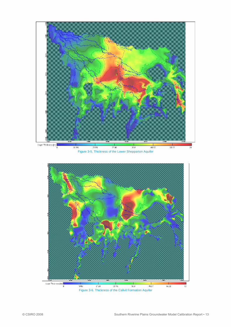
Figure 3-5. Thickness of the Lower Shepparton Aquifer

Figure 3-6. Thickness of the Calivil Formation Aquifer


Figure 3-7. Thickness of the Renmark Group Aquifer


3.2 Model input data

3.2.1 Storage parameters Table 3-2 defines the storage parameters (specific yield and specific storage) utilised in the model. The confined storage

parameter, specific storage, is defined per meter of aquifer thickness and hence the effective storage coefficient can be

obtained by multiplying the specific storage by the aquifer thickness. These values were derived through the calibration

process through which it was found that extremely small storage parameters were required to achieve the observed

levels of pumping-related drawdown in New South Wales. The issues related to matching the observed levels of

drawdown are further discussed in Section 4.2.

Table 3-2. Storage parameters defined in the model

Aquifer Aquifer type Storage parameter New South Wales Victoria

Upper Shepparton Unconfined Specific yield (Sy) 0.005 0.01

Lower Shepparton Confined Specific storage (Ss) 1 x 10-6 5 x 10-6

Calivil Confined Specific storage (Ss) 1 x 10-6 5 x 10-6

Renmark Confined Specific storage (Ss) 1 x 10-6 5 x 10-6

3.2.2 Hydrogeological conductivity values Hydraulic conductivity values are shown in Figure 3-8 through Figure 3-11.

The Shepparton Formation is characterised by variable hydraulic conductivity and this is reflected in the model

parameters. Typically horizontal conductivities range between 0.5 and 5 m/day. However, they have been modelled as

high as 75 m/day in a small pocket in the upper reaches of the Goulburn-Broken catchment. In the north of the model

area there is very little difference in vertical hydraulic conductivities between the upper and lower Shepparton Formation.

Consequently modelled layers 1 and 2 behave as one aquifer. Further south the Upper Shepparton often becomes more

hydraulically conductive and the Lower Shepparton acts as a confining layer.

The Calivil Formation and Renmark Group are both comprised of highly hydraulically conductive material. Model

horizontal hydraulic conductivities in these aquifers are typically between 50 and 100 m/day. The exception to this is in

the north-east near Jerilderie where hydraulic conductivities reduce to as low as 5 m/day.


Figure 3-8. Hydraulic conductivity values in Layer 1 (Upper Shepparton Formation)


Figure 3-9. Hydraulic conductivity values in Layer 2 (Lower Shepparton)


Figure 3-10. Hydraulic conductivity values in Layer 3 (Calivil Formation)


Figure 3-11. Hydraulic conductivity values in Layer 4 (Renmark Group)


3.2.3 Rivers and drains A large amount of river gauge data exists for all of the major rivers included within the Southern Riverine model area.

River level data was sourced from Thiess Environmental Ltd. for all Victorian gauges and Department of Water and

Energy for all New South Wales river gauges. A list of the river gauges is provided in Appendix A. Where data gaps were

present in the time series, a linear interpolation was applied from the nearest available gauge. Where previous

groundwater models were available (namely Campaspe and Lower Murray), river gauge data was sourced from these

models. The rivers included in the model are represented by the bold dark blue cells in Figure 3-12.

Only the main stems of major rivers are included in the model. As Figure 3-13 shows, this represents only a minor

percentage of all natural surface water features and an even smaller percentage when man-made drainage features are

considered. To account for tributaries and drainage channels that cannot be explicitly modelled, a number of drainage

areas were included in the model. These are represented by the shaded grey areas in Figure 3-12. Drainage cells have

only been placed in areas that are prone to shallow watertables and are designed to mimic natural or man-made

drainage features that would act to intercept rising watertables. These are particularly common in the irrigated areas of

New South Wales. In Modflow, drain cells may act only as groundwater discharge points, as opposed to river cells which

can act as both recharge and discharge sites.

The majority of surface drains (both natural and man-made) are directly hydraulically connected to the rivers. Therefore it

is recommended that when using this model to assess stream–aquifer interactions, model-predicted discharges to drains

should contribute to the total.

Figure 3-12. Rivers and drains included in the Southern Riverine model


Figure 3-13. All natural surface water features within the Southern Riverine model domain

3.2.4 Recharge (dryland and irrigation) Dryland rainfall recharge and irrigation recharge are both incorporated into the model. Of the three previous models

within the model domain, only the Campaspe model had readily replicable recharge inputs. The Katunga model utilised

constant heads across layer 1 to provide a recharge flux into the top of the model. The Lower Murray model utilised a

pilot point calibration process to define a spatially variable recharge pattern across the model. Such an approach was

deemed to be inappropriate for the current model in light of the size and resolution of the model.

Given the size of the model a methodology was developed that would provide consistency across the model domain

whilst providing a recharge input data set that could be manipulated easily in both the calibration and scenario modelling

processes. The methodology used to create the recharge data set is summarised below:

• The model domain was divided into ‘rainfall districts’ as defined by the Bureau of Meteorology (2006). These

rainfall districts define zones of similar rainfall on a resolution deemed appropriate given the model extent

(Figure 3-14).

• Areas of irrigation were identified from satellite imagery (Figure 2-1). These areas include both surface water

and groundwater derived irrigation (Figure 3-15)

• The rainfall districts and irrigation districts were superimposed onto each other creating a set of recharge zones.

• Twenty locations (rainfall sites) were identified across the model area where rainfall data was to be collated

(Figure 3-16). The rainfall sites were assigned to 24 separate recharge zones in Visual Modflow (Figure 3-17).

• Rainfall for each rainfall site was extracted from the SILO database. Rainfall was scaled to calculate dryland

rainfall recharge.

• Irrigation, where applicable, was added as a constant recharge volume between the months of November and

April inclusive. Irrigation was applied in addition to the appropriate rainfall recharge.


During calibration it became apparent that groundwater recharge was decreasing significantly in the model calibration

period (i.e. more than was occurring through the natural reduction in rainfall that has been observed throughout the

Riverine Plains). This was particularly prevalent in the northern half of the model. Thus an irrigation efficiency scaling

factor was introduced. This scaling factor accounts for the improvements in irrigation efficiency that have occurred since

the early 1990s. Significantly it is considered that the volume of irrigation water reaching the watertable has been

reduced by a number of factors including infrastructure improvements, drainage schemes and climate. As a simple

means of implementing this process, irrigation-induced groundwater recharge was assumed to decrease by 8% per year

starting in 1994 to a total reduction of 80% by 2004. This was invoked over Modflow recharge zones 2 to 7 (across the

northern half of the model).

Note: The irrigation efficiency factor was invoked in New South Wales in response to the model’s inability to match the

magnitude of observed drawdown cones, particularly in the area of Deniliquin and west toward Swan Hill. It is

acknowledged that reduced irrigation recharge may not be the only explanation for the drawdown, i.e. climate-induced

variations and inaccuracies in the metered pumping estimates may also have contributed to this. It is likely that the

drawdown is attributable to all three explanations. However, in light of available data the most acceptable calibration

scaling tool was deemed to be the irrigation accessions.

Table 3-3 displays the recharge zones, land use, irrigation intensity, rainfall scaling factors and average annual recharge

for the period 1990 to 2006.


Table 3-3. Southern Riverine modelled recharge zones

Modflow recharge zone

SILO rainfall site Land use Irrigation zone Irrigation Rainfall scaling factor

Average annual recharge

mm/y mm/y

1 - - - - - -

2 2 Medium irrigation Mulwala Canal 30 0.008 18.05

3 3 Low irrigation 15 0.008 10.58

4 4 Medium irrigation Wakool 30 0.008 18.01

5 5 High irrigation Wakool 100 0.04 62.79

6 6 Dryland 0.008 2.63

7 7 Medium irrigation Swan Hill 30 0.02 16.61

8 7 Dryland 0.02 6.61

9 8 Dryland 0.02 7.68

10 9 Medium irrigation Loddon 25 0.03 23.11

11 9 Medium irrigation Barham 30 0.02 17.08

12 10 Dryland 0.045 18.80

13 11 Dryland 0.045 16.59

14 12 Dryland 0.10 42.19

15 13 High irrigation Campaspe 45 0.01 26.56

16 14 Dryland 0.02 9.11

17 15 Dryland 0.02 8.35

18 16 High irrigation Shepparton 45 0.04 40.62

19 17 High irrigation Katunga 60 0.04 46.95

20 18 High irrigation Goulburn-Broken 60 0.02 24.36

21 19 Dryland 60 0.04 20.89

22 20 Dryland 0.02 9.90

23 1 Very low irrigation

5 0.008 6.09

24 3 Forest 0.005 1.92


Figure 3-14. Rainfall districts as defined by the Bureau of Meteorology (2006)

Figure 3-15. Satellite imagery highlighting irrigation areas incorporated into the Southern Riverine model


Figure 3-16. Rainfall sites (1 to 20) input into the Waves Model to deduce dryland recharge variability across the model


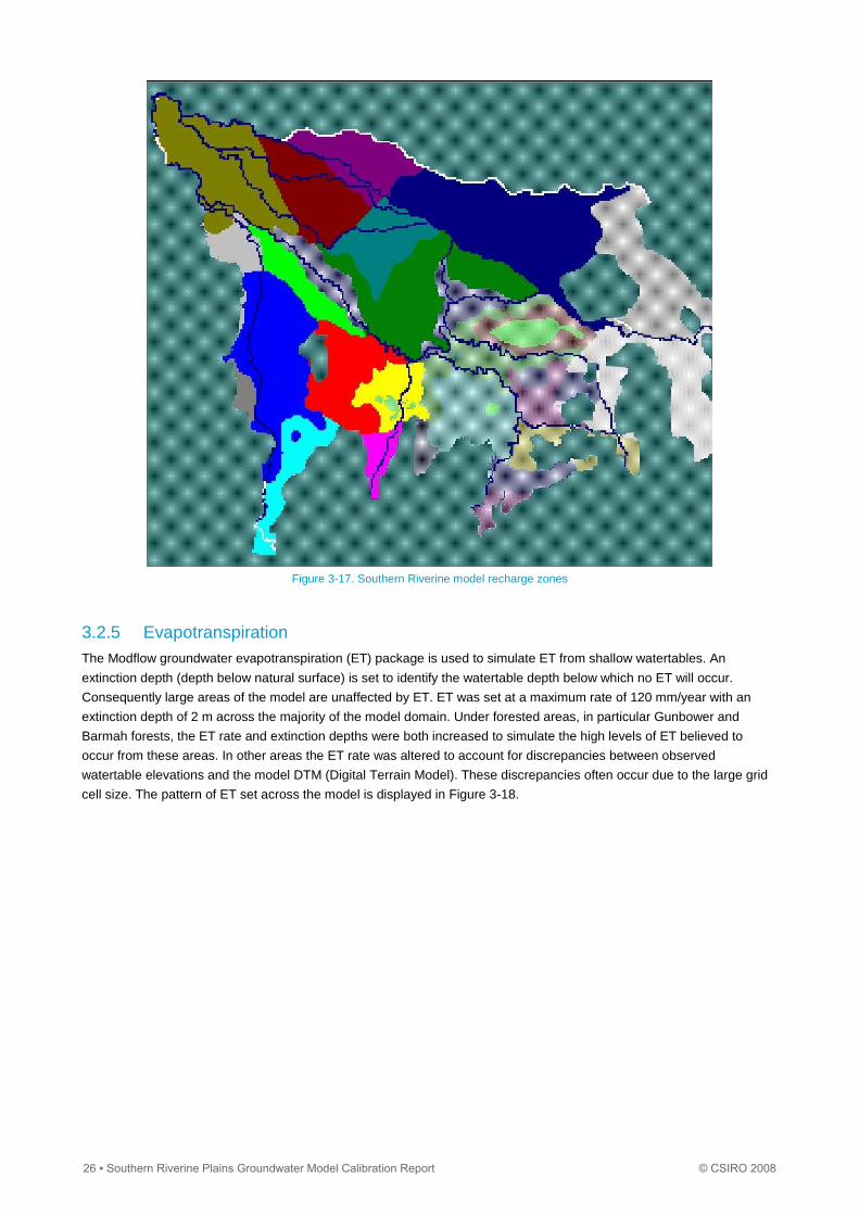
Figure 3-17. Southern Riverine model recharge zones

3.2.5 Evapotranspiration The Modflow groundwater evapotranspiration (ET) package is used to simulate ET from shallow watertables. An

extinction depth (depth below natural surface) is set to identify the watertable depth below which no ET will occur.

Consequently large areas of the model are unaffected by ET. ET was set at a maximum rate of 120 mm/year with an

extinction depth of 2 m across the majority of the model domain. Under forested areas, in particular Gunbower and

Barmah forests, the ET rate and extinction depths were both increased to simulate the high levels of ET believed to

occur from these areas. In other areas the ET rate was altered to account for discrepancies between observed

watertable elevations and the model DTM (Digital Terrain Model). These discrepancies often occur due to the large grid

cell size. The pattern of ET set across the model is displayed in Figure 3-18.


Figure 3-18. Groundwater evapotranspiration rates set across the Southern Riverine model

3.2.6 Boundary conditions Groundwater flow is typically in a northwesterly direction, approximately following the drainage path of the Murray River.

Consequently to allow for movement of groundwater out of the model domain, general head boundaries were included in

the north-west corner of the model (Figure 3-19). These boundaries were added to the model in the Lower Shepparton,

Calivil and Renmark aquifers (layers 2, 3 and 4 respectively). All other model boundaries were designated as no flow

boundaries as the majority of the area is bordered by outcropping bedrock. The one exception was in the north and

north-east where despite the lack of a physical barrier to groundwater movement a no flow boundary is still used. The

key reasons for this are as follows:

• Groundwater flow under the northern boundary is typically in a westerly direction (i.e. parallel to the boundary).

Consequently it is conceptualised that there is little flow of water across this boundary.

• The extent of interference effects from the aquifers in the neighbouring Murrumbidgee catchment is unclear.

Including a general head boundary in this part of the Southern Riverine model would predispose the model to

draw water from the neighbouring aquifer under prolonged pumping. In light of the fact that a similar

groundwater model has been developed for the Lower Murrumbidgee aquifer it is considered inappropriate that

both models can source water from across the common boundary. Given the uncertainty involved (and the

nature of the scenario modelling in this project which aims to run to dynamic equilibrium) it was deemed more

appropriate to allocate a no flow boundary. In doing so, groundwater recharge is restricted to ‘real’ processes

such as rainfall and river leakage occurring within the model domain, as opposed to recharge processes that

may occur outside the model domain.


Two additional general head boundaries were added to small sections in the Campaspe Deep Lead (not shown) and

Mid-Goulburn (shown below). These were used to simulate groundwater movement between the Deep Lead and the

bedrock.

Figure 3-19. General head boundaries


4 Model calibration

4.1 Calibration method

The model was calibrated in transient mode by matching model-predicted groundwater responses to measured

groundwater hydrographs in a series of observation bores spread across the model domain. The calibration model was

constructed using monthly stress periods from January 1990 to December 2005 (16 years, 192 months). A relatively

short calibration period was selected for the following reasons:

• Due to the size of the model, run times were a key consideration. Therefore a shorter calibration period was

preferred.

• From the mid-1990s and peaking in 2002/03 there was significant development of the groundwater resources in

the model domain which saw usage increase from under 100 GL/year to over 400 GL/year. By including this

period the model is calibrated over both low and high groundwater usage conditions.

An iterative approach was used to refine model parameters in order to optimise the match to observed water levels.

Priorities of the calibration were to achieve the following:

• reproduction of the long-term trends in observation bore hydrographs (in particular long-term drawdown trends)

• appropriate representation of vertical hydraulic gradients at nested bore sites

• accurate representation of river interactions via the matching of seasonal fluctuations in shallow watertable

bores located near the major rivers.

The calibration model was evaluated based on four criteria as specified in the Murray-Darling Basin Commission

Groundwater Flow Modelling Guidelines (Middlemis, 2000). These criteria are summarised in Table 4-1.

Table 4-1. Calibration model performance criteria (after Middlemis, 2000)

Performance measure Criteria

Water balance A value of less than 1% should be obtained for the water balance error term for each stress period and cumulatively for the entire simulation.

Iteration residual error Iteration convergence criterion should be one to two orders of magnitude smaller than the level of accuracy desired in the model head results. Commonly set in the order of millimetres or centimetres.

Qualitative measures Subjective assessment of the goodness of fit between modelled and measured groundwater level contour plans and hydrographs of bore water levels and surface flows. Justification for adopted model aquifer properties in relation to measured ranges of values and associated non-uniqueness issues.

Quantitative measures Residual head statistics criteria (specifically the Normalised Root Mean Squared, RMS). Given the intermediate model complexity a normalised RMS less than 10% is considered acceptable. Consistency between modelled head values (in contour plans and scatter plots) and spot measurements from monitoring bores. Comparison of simulated and measured components of the water budget, notably surface water flows, groundwater abstractions and evapotranspiration estimates.

4.1.1 Groundwater extraction The following section is reported by state in reference to the differing groundwater data sources.

New South Wales groundwater extraction data

Historical estimates of groundwater extractions have previously been compiled as part of the existing Lower Murray

(GWMA 016) groundwater model. This data covered the period 1985 to 2000. Metered groundwater usage data for the

period 1999/00 to 2005/06 was provided by the New South Wales Department of Natural Resources to allow the

extension of the data to cover the Southern Riverine model calibration period. Metered data has its own limitations in that

it may not represent the total volume pumped from the aquifer (i.e. it may not include all extraction sites). In recognition

of the limitations with groundwater usage data a methodology was developed to allow for extraction data to be scaled


such that the total annual usage for all extraction bores included in the model corresponds with the best estimates of

annual groundwater usage. This methodology is as follows:

• Total annual pumping at each bore is calculated based on available data from the Lower Murray model and

recent metered data.

• An initial total annual pumping volume is calculated for all bores.

• Best estimates of actual groundwater usage were provided by the New South Wales Department of Natural

Resources (Table 4-2 and Figure 4-1).

• All groundwater bores are scaled such that the modelled groundwater usage equals the best estimates of actual

groundwater usage.

• The annual total of groundwater usage at every bore was distributed into a monthly time series. This distribution

followed that utilised in the Lower Murray Groundwater Model (DLWC, 2001) as shown in Figure 4-2.

Table 4-2. Estimated groundwater usage in New South Wales (supplied by the New South Wales Department of Natural Resources)

Financial year GWMA016 (Deep Lead) Shepparton

ML/y

1989/90 8100 29000

1990/91 10800 35500

1991/92 13500 34500

1992/93 13500 35000

1993/94 13500 34500

1994/95 20250 35000

1995/96 21600 34000

1996/97 33750 33500

1997/98 43200 33500

1998/99 37777 33500

1999/00 71563 33500

2000/01 49139 33500

2001/02 66141 33500

2002/03 121433 33500

2003/04 67342 33500

2004/05 68134 33500

2005/06 54086 33500

0

20

40

60

80

100

120

140

160

180

1989/90 1991/92 1993/94 1995/96 1997/98 1999/00 2001/02 2003/04 2005/06

Gro

un

dw

ate

r U

sag

e (

GL

/yr)

. NSW - Deep Lead

NSW - Shepparton

Figure 4-1. Estimated volumes of groundwater extractions in New South Wales


0

2

4

6

8

10

12

14

16

18

Jul Aug Sep Oct Nov Dec Jan Feb Mar Apr May Jun

Percent of Groundwater Pumping

Figure 4-2. Distribution of groundwater pumping throughout a calendar year

Victorian groundwater extraction data

Groundwater extraction data for the Victorian half of the model was provided by Goulburn-Murray Water (GMW). A

summary of the data provided follows:

• all available metered groundwater usage data. This includes metered bores from Campaspe Deep Lead WSPA,

Katunga WSPA, Shepparton WSPA, Kialla GMA, Mid-Goulburn GMA and Mid-Loddon GMA. Metered data

usually covered the period from 1999/00 to 2005/06

• a list of all licensed groundwater extraction bores within the GMW area including licensed volumes

• estimated groundwater usage as a percentage of total licensed volume for each GMA (or WSPA) and for all

unincorporated areas

• lists of ‘active’ and ‘sleeper’ licences within each GMA.

As per the New South Wales data it was not possible to source accurate groundwater usage for every bore on a monthly

time step for the whole calibration period (1990 to 2006). Most records of metered data only began around 1999 and

there remains a large number of bores that are not metered, both outside and within GMA boundaries. Consequently a

methodology was suggested by GMW to estimate the actual groundwater usage from each bore. This methodology is

summarised as follows:

• Bore construction dates for all licensed extraction bores were extracted from the Victorian Groundwater

Management System database.

• The bore construction date is assumed to be the year in which the groundwater licence is issued and

groundwater pumping commenced.

• The total licensed volume for each GMA, WSPA and the unincorporated areas for each year within the

calibration period was calculated.

• Actual metered groundwater usage data was collated where available.

• In years, or areas, where metered data was not available, GMW provided estimated groundwater usage as a

percentage of total licensed volume.

• The total licensed volumes for each bore was scaled such that the total modelled volume of usage equalled the

total metered volume or the estimated total use.

Final groundwater usage estimates are provided in Table 4-3, Table 4-4 and Figure 4-3. A map of all groundwater

extraction sites is provided in Figure 4-4.


Table 4-3. Groundwater usage estimates in Victorian groundwater management units

Area Campaspe Deep Lead

Goorambat Katunga Kialla Mid-Goulburn

Mid-Loddon Ellesmere Shepparton Total (incl NSW)

ML/y

1989/90 0 379 10,432 1,281 1,091 8,222 170 39,477 96,837

1990/91 0 379 11,076 1,281 1,094 8,526 170 40,207 107,020

1991/92 0 386 11,151 1,281 1,094 8,526 170 41,451 109,346

1992/93 3,341 386 11,161 1,281 1,094 8,911 170 42,619 114,749

1993/94 11,383 386 11,500 1,286 1,188 8,931 170 43,868 123,999

1994/95 15,570 543 17,653 1,286 1,689 11,492 351 76,987 176,673

1995/96 13,261 426 14,977 1,286 1,338 9,194 251 47,456 138,975

1996/97 19,335 631 20,100 1,407 1,490 9,238 251 126,428 238,166

1997/98 18,235 568 31,122 1,424 2,304 11,789 351 83,702 216,113

1998/99 14,865 426 23,101 1,424 2,150 9,640 251 53,375 195,544

1999/00 22,103 655 28,645 1,435 2,192 9,482 351 127,880 289,312

2000/01 15,373 568 22,795 1,424 2,192 7,383 351 70,566 176,405

2001/02 26,461 781 28,873 1,424 2,923 14,274 451 126,645 293,806

2002/03 31,059 781 40,470 1,424 2,482 18,435 1,588 186,921 436,588

2003/04 23,931 568 24,285 854 4,120 14,095 2,273 62,355 225,480

2004/05 26,089 574 25,660 862 3,596 15,580 2,521 70,035 238,795

2005/06 23,456 568 21,614 854 3,491 15,832 3,188 94,932 242,206

Average 15,557 530 20,860 1,266 2,090 11,150 443 78,524 201,177

Table 4-4. Groundwater usage estimates for Victorian unincorporated areas (grouped by catchment)

Area Avoca Broken Campaspe Goulburn Loddon Ovens Total

1989/90 35 123 121 49 329 312 968

1990/91 35 123 121 49 329 324 980

1991/92 35 123 121 49 374 324 1,025

1992/93 35 128 121 52 374 324 1,033

1993/94 35 128 121 52 374 324 1,033

1994/95 49 185 349 73 523 453 1,632

1995/96 35 137 284 52 592 324 1,423

1996/97 35 137 371 52 592 338 1,525

1997/98 49 207 519 73 1,188 571 2,606

1998/99 35 151 381 71 863 508 2,009

1999/00 49 211 533 99 1,209 724 2,825

2000/01 49 227 533 113 1,209 734 2,864

2001/02 63 301 1,022 145 1,554 943 4,028

2002/03 63 303 1,022 147 2,249 1,312 5,096

2003/04 49 239 797 116 2,695 1,039 4,934

2004/05 49 244 797 117 2,723 1,039 4,968

2005/06 49 259 832 117 2,724 1,041 5,020

Average 44 190 473 84 1,170 625 2,586


0

50

100

150

200

250

300

350

1989/90 1991/92 1993/94 1995/96 1997/98 1999/00 2001/02 2003/04 2005/06

Gro

undw

ater

Usa

ge (

GL/

yr)

.UnincorporatedMurmungeeEllesmereMid-GoulburnKiallaGoorambatMid-LoddonCampaspe Deep LeadKatungaShepparton

Figure 4-3. Estimated groundwater usage in the Victorian groundwater management units and unincorporated areas

Figure 4-4. Groundwater extraction wells included in the Southern Riverine model

Note: Groundwater extraction wells in New South Wales appear to line up in rows and columns. This is an artefact of the import of the wells from the existing Lower Murray groundwater model that was constructed on a 2.5 km grid (DLWC, 2001).


4.1.2 Calibration model observation bores In total 142 monitoring wells were utilised in the calibration of the Southern Riverine model. Many of these are nested

water level observation sites where water levels from different aquifer depths are monitored at the one location.

Calibration bores cover the entire model domain in all layers (Figure 4-5 to Figure 4-8). A list of all observation bores,

including coordinates and aquifer screened, is also included in Appendix B.

Figure 4-5. Observation bores screening the Upper Shepparton


Figure 4-6. Observation bores screening the Lower Shepparton

Figure 4-7. Observation bores screening the Calivil Formation


Figure 4-8. Observation bores screening the Renmark Group

4.2 Calibration model results

All calibration model hydrographs are presented in Appendix C. Potentiometric surface comparisons and calibration

statistics are provided in Section 4.5.

4.3 Summary of hydrographs by region

4.3.1 Murray The calibration in the Murray region attempted to match the magnitude of observed drawdown that occurred during the

period from the mid-1990s to approximately 2004/05. This drawdown is considered to be a consequence of below-

average rainfall in the region combined with large increases in deep lead pumping during the period. Through

manipulation of hydraulic parameters alone it proved very difficult to achieve both the depth and breadth of the drawdown

cone (centred near Deniliquin). As previously explained in Section 3.2.4, an irrigation efficiency factor was introduced to

reduce the net recharge in the Lower Murray region and subsequently induce greater drawdown. This proved effective.

However, it is acknowledged that the rate and magnitude of observed drawdown is not completely achieved in the final

calibrated model. An example of this is provided in Figure 4-9 where the rate of observed drawdown is greater than the

rate of calculated drawdown. This example also depicts the model’s preferential calibration to the later time data which

provides a closer fit than data from the early 1990s. This outcome is consistent with general queries raised as to the

accuracy of the earlier extraction data (M. Williams, DWE, pers. comm.).

In the east near Jerilderie, there is a distinctive rising trend in water levels, particularly in the Shepparton Formation. The

model reproduces these rising trends with reasonable accuracy as shown in Figure 4-10.

An additional hydrogeological pattern that the model attempted to preserve was a significant shift in the head difference

between the Upper Shepparton and the deeper aquifers. This is observed as falling heads in the deep aquifers in


contrast to relatively stable heads in the Upper Shepparton (often restricted by drainage and shallow pumping). This

occurs at many locations throughout the Murray region, in particular in the south near Echuca (refer to example in Figure

4-11).

In the Gunbower Forest area the calibration process highlighted the importance of forest evapotranspiration. The

introduction of an increased rate of evapotranspiration and deeper extinction resulted in a good calibration across most

of the forested area (Figure 4-12). In this area observed hydrographs depict relatively stable water levels with a slight

downward trend from the mid-1990s. Calculated hydrographs generally represent this pattern well. Where inaccuracies

occurred, this was typically in the Shepparton Formation and believed to be a result of steep hydraulic gradients along

the river which makes accurate modelling at this scale difficult.

In the north of the Loddon catchment, near the Murray River, observed hydrographs depict relatively stable water levels

with a slight downward trend from the mid-1990s. This is generally well reproduced in the model. At one nested site (see

Figure 4-13) a complex relationship between the formations is observed. This site shows heads in the Lower Shepparton

consistently higher than both the Upper Shepparton and the Renmark Group aquifer. This is not observed elsewhere in

the Loddon region and may indicate a bore failure. The modelled levels indicate minimal variation in heads between

layers. Bore 76761 in the north-east of the region (toward Gunbower Forest) displays a trend after 2000 that may

suggest the impacts of groundwater pumping from further west and/or north-west.

The Katunga WSPA, representing approximately 10% of total usage in the Victorian half of the model, has some of the

largest drawdowns (both seasonal and long-term) in the region. Fortunately this area also has a large amount of reliable

data available via metering and previous studies (e.g. GMW, 2006a). Consequently a good correlation was achieved

between observed and modelled hydrographs, particularly in the Deep Lead. However, the same level of correlation was

not obtained in the watertable aquifer (Figure 4-15). This is likely to be a product of the complex variability (in time and

space) of irrigation schemes combined with extensive shallow pumping and drainage for salinity control purposes that

are difficult to replicate in the regional model.

65

70

75

80

85

90

95

1990 1993 1996 1999 2002 2005

Red

uced

Wat

er L

evel

(m

AH

D)

36744 - Layer 2 (CAL)

36744 - Layer 2 (OBS)

36743 - Layer 4 (CAL)

36743 - Layer 4 (OBS)

36742 - Layer 3 (CAL)

36742 - Layer 3 (OBS)

Figure 4-9. Example hydrographs from the Murray region near Deniliquin (note: this is not a nested site)


100

102

104

106

108

110

112

114

116

118

120

1990 1993 1996 1999 2002 2005

Red

uced

Wat

er L

evel

(m

AH

D)

36391 - Layer 1 (CAL)

36391 - Layer 1 (OBS)

36351 - Layer 1 (CAL)

36351 - Layer 1 (OBS)

36350 - Layer 1 (CAL)

36350 - Layer 1 (OBS)

Figure 4-10. Example hydrographs from the Murray region in the east between Corowa and Jerilderie

70

72

74

76

78

80

82

84

86

88

90

1990 1993 1996 1999 2002 2005

Red

uced

Wat

er L

evel

(m

AH

D)

36765 - Layer 3 (CAL)

36765 - Layer 3 (OBS)

36644 - Layer 1 (CAL)

36644 - Layer 1 (OBS)

Figure 4-11. Example hydrographs from the Murray region in the south near Echuca


60

62

64

66

68

70

72

74

76

78

80

1990 1993 1996 1999 2002 2005

Red

uced

Wat

er L

evel

(m

AH

D)

36162 - Layer 4 (CAL)

36162 - Layer 4 (OBS)

36161 - Layer 4 (CAL)

36161 - Layer 4 (OBS)

Figure 4-12. Example hydrographs from the Murray region in Gunbower Forest

60

62

64

66

68

70

72

74

76

78

80

1990 1993 1996 1999 2002 2005

Red

uced

Wat

er L

evel

(m

AH

D)

82759 - Layer 1 (CAL)

82759 - Layer 1 (OBS)

82758 - Layer 2 (CAL)

82758 - Layer 2 (OBS)

82757 - Layer 4 (CAL)

82757 - Layer 4 (OBS)

Figure 4-13. Example hydrographs from the north of the Loddon catchment in the Murray region


70

72

74

76

78

80

82

84

86

88

90

1990 1993 1996 1999 2002 2005

Red

uced

Wat

er L

evel

(m

AH

D)

76761 - Layer 1 (CAL)

76761 - Layer 1 (OBS)

Figure 4-14. Example hydrographs from the north-east of the Loddon catchment in the Murray region

70

75

80

85

90

95

100

105

110

1990 1993 1996 1999 2002 2005

Red

uced

Wat

er L

evel

(m

AH

D)

97613 - Layer 3 (CAL)

97613 - Layer 3 (OBS)

97614 - Layer 1 (CAL)

97614 - Layer 1 (OBS)

Figure 4-15. Example hydrographs from the Katunga WSPA within the Murray region

4.3.2 Loddon-Avoca With the exception of the northern end of the Mid-Loddon GMA, the Loddon-Avoca region generally has poor spatial

coverage of observation bores. This is a result of the lack of groundwater development north of the GMA due to the poor

quality groundwater in the region.

In the Mid-Loddon GMA the calibration was aimed at matching drawdowns observed since the mid-1990s, a result of

climate and increasing extractions (Figure 4-16). This was replicated at all sites except for nested site 88239 and 88214

(Figure 4-17) which was anomalous in that the observed hydrographs did not show the same level of long-term


drawdown as observed elsewhere in the GMA. It is likely that this is a result of localised conditions (possibly irrigation-

induced mounding) that could not be replicated in a regional model.

100

102

104

106

108

110

112

114

116

118

120

1990 1993 1996 1999 2002 2005

Red

uced

Wat

er L

evel

(m

AH

D)

36416 - Layer 1 (OBS)

36416 - Layer 1 (CAL)

36415 - Layer 2 (OBS)

36415 - Layer 2 (CAL)

Figure 4-16. Example hydrographs from the Mid-Loddon GMA

90

95

100

105

110

115

120

1990 1993 1996 1999 2002 2005

Red

uced

Wat

er L

evel

(m

AH

D)

88239 - Layer 1 (CAL)

88239 - Layer 1 (OBS)

88214 - Layer 3 (CAL)

88214 - Layer 3 (OBS)

Figure 4-17. Example hydrographs from the Mid-Loddon GMA

4.3.3 Campaspe The significant levels of long-term drawdown observed in the Deep Lead aquifer and the relatively static watertable levels

were the focus of calibration in the Campaspe region. A good example of this is shown in the hydrographs in Figure 4-18

(near Echuca) where the model replicates this trend well. At a number of sites the model was under estimating the level


of seasonal drawdown – however, the long-term drawdown was being reproduced (e.g. Figure 4-19). The inability to

reproduce the seasonal drawdown was considered to be of lesser importance to the long-term trend.

Accurate calibration became more difficult toward the south, where natural surface elevations and watertables change

rapidly (adjacent cells can have elevation differences of 20 m or greater). The Deep Leads in the south are also prone to

increasing interference from localised processes that are not represented in a regional model. Nevertheless, long-term

trends have generally been preserved despite the model not achieving some of the seasonal drawdown levels observed

in some of the hydrographs (e.g. Figure 4-20).

70

75

80

85

90

95

100

1990 1993 1996 1999 2002 2005

Red

uced

Wat

er L

evel

(m

AH

D)

79324 - Layer 4 (CAL)

79324 - Layer 4 (OBS)

79329 - Layer 1 (CAL)

79329 - Layer 1 (OBS)

Figure 4-18. Example hydrographs from the Campaspe region near Echuca

65

70

75

80

85

90

95

100

105

110

1990 1993 1996 1999 2002 2005

Red

uced

Wat

er L

evel

(m

AH

D)

47253 - Layer 4 (CAL)

47253 - Layer 4 (OBS)

47251 - Layer 1 (CAL)

47251 - Layer 1 (OBS)

Figure 4-19. Example hydrographs from the Campaspe region


110

112

114

116

118

120

122

124

126

128

1990 1993 1996 1999 2002 2005

Red

uced

Wat

er L

evel

(m

AH

D)

62595 - Layer 3 (CAL)

62595 - Layer 3 (OBS)

62599 - Layer 2 (CAL)

62599 - Layer 2 (OBS)

Figure 4-20. Example hydrographs from the Campaspe region

4.3.4 Goulburn-Broken The southern extents of the Goulburn-Broken region proved to be the most difficult region to calibrate, largely due to the

very steep topographic gradients (and similarly steep groundwater level gradients). The Modflow groundwater modelling

package is prone to becoming highly unstable in such terrain and particularly where there is a large groundwater gradient

between adjacent cells. In the area near Goulburn Weir this proved to be a particular problem where attempts to force

steep gradients often resulted in model convergence failures. An example of this is shown in Figure 4-21 where the steep

gradients observed between bores 79909 and 79908 were not able to be preserved due to model stability issues.

Another site particularly prone to this problem was bore 98132 which is located next to a bedrock high. Elsewhere in the

Goulburn-Broken region, particularly in the flatter areas of the north, a generally good calibration was reached with trends

similar to those seen in the Campaspe and Katunga WSPAs (Figure 4-22 and Figure 4-23).


105

107

109

111

113

115

117

119

121

123

125

1990 1993 1996 1999 2002 2005

Red

uced

Wat

er L

evel

(m

AH

D)

58268 - Layer 1 (CAL)

58268 - Layer 1 (OBS)

79908 - Layer 3 (CAL)

79908 - Layer 3 (OBS)

79909 - Layer 1 (CAL)

79909 - Layer 1 (OBS)

Figure 4-21. Example hydrographs from the Goulburn-Broken region

85

90

95

100

105

110

115

1990 1993 1996 1999 2002 2005

Red

uced

Wat

er L

evel

(m

AH

D)

61675 - Layer 3 (CAL)

61675 - Layer 3 (OBS)

61683 - Layer 1 (CAL)

61683 - Layer 1 (OBS)



100

102

104

106

108

110

112

114

116

118

120

1990 1993 1996 1999 2002 2005

Red

uced

Wat

er L

evel

(m

AH

D)

70237 - Layer 3 (CAL)

70237 - Layer 3 (OBS)

46195 - Layer 2 (CAL)

46195 - Layer 2 (OBS)

46190 - Layer 3 (CAL)

46190 - Layer 3 (OBS)


4.4 Potentiometric surface maps

Maps comparing observed versus modelled potentiometric surfaces have been used to ensure the model is adequately

representing the intermediate to regional scale flow systems. The maps are presented in Figure 4-24 through to Figure

4-27. These present potentiometric surfaces from both the Shepparton Formation and the Deep Lead at two separate

times during the calibration period:

• March 1995, five years into the calibration period. This time was selected as it is far enough from the start of the

model run such that any model instabilities at initialisation should have decayed. It is also the start of the period

when there was significant growth in the use of the groundwater resource across the model domain.

• May 2003, near the end of the calibration period. This time represents the period in which drawdown is at its

greatest during the calibration period. After this time groundwater levels typically started to flatten out (possibly

approaching equilibrium).

Note: These surfaces were created by contouring data from the model observation bores (Section 4.1.2). Areas with little

spatial coverage of observation bores (such as the Loddon catchment) will be less accurate than areas with a good

spatial coverage of bores (such as the Campaspe and Katunga WSPAs).

Overall the modelled potentiometric surfaces indicate a reasonable match to the observed levels. Importantly the

intermediate and regional scale flow processes have been reproduced in both the Shepparton Formation and the Deep

Lead aquifer. Typically the highest deviations between the observed and modelled levels occur near the model

boundaries. This is due to limitations in modelling boundary conditions, in particular the preference to avoid using non-

time varying boundary conditions.


4.4.1 Shepparton Formation

Figure 4-24. Comparison of observed and modelled watertables (Shepparton Formation) based on data from March 1995

Figure 4-25. Comparison of observed and modelled watertables (Shepparton Formation) based on data from May 2003


4.4.2 Deep Lead

Figure 4-26. Comparison of observed and modelled potentiometric surfaces (Deep Lead) based on data from March 1995

Figure 4-27. Comparison of observed and modelled potentiometric surfaces (Deep Lead) based on data from May 2003


4.5 Calibration statistics

In large models such as this, calibration statistics are typically considered to be less important than matching

hydrographs and potentiometric surfaces. This is because calibration statistics such as correlation co-efficients tend to

‘flatter’ models with large numbers of observation wells and also large variations in elevation across the model domain.

The calibration statistics for the Southern Riverine fall into this category. Therefore, during the calibration process,

attention was specifically focused on matching observed hydrographs. Nevertheless, the calibration results presented in

Table 4-5 and Figure 4-28 indicate a model that is generally well calibrated even when separated by layer or by region.

Figure 4-28 also indicates that there is no significant deviation throughout the model run (i.e. there is no particular period

during the calibration run when the model is performing particularly poorly). These statistics are well within the

performance criteria specified in Section 4.1.

Table 4-5. Calibration model statistics

Zone Number of observation wells

RMS (m) Normalised RMS (%) Correlation co-efficient

All 142 2.23 1.76 0.99

Layer

Upper Shepparton 61 2.19 1.73 0.99

Lower Shepparton 26 1.80 2.85 0.99

Calivil Formation 31 2.15 3.00 0.99

Renmark Formation 24 2.73 4.48 0.98

Region

New South Wales 35 1.65 2.36 0.99

Loddon 18 1.92 1.67 0.99

Campaspe 14 2.94 3.95 0.99

Goulburn-Broken 53 2.57 3.88 0.98

Katunga 12 2.74 5.75 0.97

0

0.5

1

1.5

2

2.5

3

1990 1993 1996 1999 2002 2005

Normalised RMS ( % )

Figure 4-28. Calibration model normalised RMS (%) over the length of the calibration period

4.6 Calibration model water balance

4.6.1 Overview The dominant groundwater recharge sources throughout the Southern Riverine Plains are low to high intensity irrigation

of large areas across the plains and rainfall infiltration recharge in the southern highlands. There is minimal lateral


groundwater flow into the model as the area is largely bordered by bedrock. However, river leakage is an important

recharge mechanism (Figure 4-29).

Across the plains groundwater evapotranspiration becomes an important discharge mechanism, particularly under

forested areas such as Gunbower and the Barmah Forest. Groundwater evapotranspiration is also important under

zones of shallow watertables which are often induced by intensive irrigation. Significant volumes of groundwater also

flow out from the model domain toward the north-west, approximately following the flow direction of the Murray River.

Refer to Figure 4-30 for a volumetric summary of groundwater discharge mechanisms.

The groundwater resource was significantly developed from the mid-1990s, particularly in relation to the deeper aquifers.

Accordingly groundwater extraction from pumping wells became an increasingly important component of the water

balance during the calibration period. As highlighted in Figure 4-31 groundwater extractions for the total area more than

tripled from the early 1990s to its maximum in 2002/03. Impacts of this trend were compounded by decreases in total

groundwater recharge1 driven mostly by climate (including decreases in high streamflow events such as bankfull and

overbank events) but also by improvements in irrigation efficiency.

0

100

200

300

400

500

600

Lateral GW Flow River Leakage Rainfall & IrrigationRecharge

Storage In

Ave

rage

Flu

x (G

L/yr

) .

Groundwater Recharge Processes

Figure 4-29. Average annual groundwater recharge (GL/year) for the calibration model (January 1990 to December 2005)

0

100

200

300

400

500

600

Lateral GW Flow Pumping Surface Drainage Discharge to River Evapotranspiration Storage Out

Ave

rage

Flu

x (G

L/yr

)

Groundwater Discharge Processes

Figure 4-30. Average annual groundwater discharge (GL/year) for the calibration model (January 1990 to December 2005)

1 Total groundwater recharge is the sum of rainfall, irrigation, river leakage and lateral groundwater flow in.


0

20

40

60

80

100

120

140

160

180

1990 1992 1994 1996 1998 2000 2002 2004

Mon

thly

Flu

x (G

L/m

onth

) .

Total Recharge

Pumping

Figure 4-31. Total groundwater extractions compared to total recharge (rainfall, irrigation, river leakage and lateral groundwater flow in)

4.6.2 Surface–groundwater interaction Figure 4-32 and Figure 4-33 present time series data of the river interactions. One of the immediately apparent features

is the significant reduction in high flow events after 1997. The high flow events in the early part of the record resulted in

significant volumes of water recharging the groundwater systems. Then in the months following the flood peak there is a

reversal in the hydraulic gradient and significant volumes of groundwater are discharged to the river systems. This

ecologically important process has all but ceased after 1997.

Whilst the major impacts of climate are obvious, the reduced levels of surface–groundwater interaction also coincide with

a period of intense groundwater development where extractions increased from approximately 150 GL in 1995/96 to

approximately 450 GL in 2002/03. The combined impact of increased pumping and a drier climate has altered the state

of stream–aquifer interactions across the region. This is observed in the slight downward trend in groundwater

discharges to rivers after 1997 and the slight upward trend in river leakage. These results are directly attributable to

reduced groundwater levels across the region.

These trends are not as severe as observed elsewhere in the Murray-Darling Basin. This is a result of intensive irrigation

causing shallow groundwater mounding in many areas within the Riverine Plains.


0

20

40

60

80

1990 1992 1994 1996 1998 2000 2002 2004

Net

Flu

x (G

L/m

onth

) .

River Leakage

Discharge to River

Figure 4-32. Time series of river leakage and groundwater discharges to the river

-50

-25

0

25

50

75

100

1990 1992 1994 1996 1998 2000 2002 2004Net

Flu

x (G

L/m

onth

) .

Net River Loss (incl. Surface Drainage)

Net River Loss

Pumping

Figure 4-33. Time series of net river losses compared to total pumping


4.7 Groundwater management unit water balances

A map locating all the GMUs within the model has previously been provided in Figure 2-4.

Table 4-6 presents average annual groundwater fluxes for each groundwater management unit within the model domain.

This data is averaged over the entire calibration period from January 1990 to December 2005. Charts showing this data

for each GMU are presented in Figure 4-34 through to Figure 4-43. Under all scenarios the difference between total

inflows and total outflows is either zero or 0.1 GL/year. This falls well within the model water balance performance criteria.

Table 4-6. Average annual groundwater inflows and outflows for each groundwater management unit within the model area

(January 1990 to December 2005)

Storage Recharge Rivers Flow across model

boundary

Flow across GMU

boundary

Leakage between aquifers

Pumping Drains EVT TOTAL

GL/y

Groundwater Inflows – Recharge

Shepparton WSPA 89.1 167.2 53.2 n/a 11.4 3.1 n/a n/a n/a 324.0

Campaspe Deep Lead

0.6 0.2 0.0 15.7 13.1 14.3 n/a n/a n/a 43.9

Mid-Goulburn 0.1 0.2 0.0 0.1 0.0 7.6 n/a n/a n/a 8.0

Kialla 0.2 0.0 0.0 n/a 5.5 12.0 n/a n/a n/a 17.6

Mid-Loddon 11.0 27.0 2.9 n/a 2.5 n/a n/a n/a n/a 43.3

Katunga 1.2 0.0 0.0 n/a 25.7 13.8 n/a n/a n/a 40.7

NSW GWMA 016 12.7 2.3 0.2 43.0 118.4 108.1 n/a n/a n/a 284.6

NSW Shepparton 71.9 197.4 86.6 0.1 6.3 46.8 n/a n/a n/a 409.0

Ellesmere 0.5 1.8 0.3 0.0 2.4 n/a n/a n/a n/a 4.9

Goorambat 0.3 1.5 1.3 n/a 0.1 n/a n/a n/a n/a 3.2

Unincorporated areas, Shepparton

34.0 111.6 42.3 3.4 29.2 n/a n/a n/a n/a 220.5

Unincorporated areas, Deep Lead

2.1 0.0 0.0 14.6 155.2 n/a n/a n/a n/a 171.9

Groundwater Outflows – Discharge

Shepparton WSPA 77.8 n/a 26.1 n/a 16.4 34.7 71.7 18.2 79.1 324.0

Campaspe Deep Lead

0.5 n/a 0.0 10.7 18.8 0.2 13.7 n/a n/a 43.9

Mid-Goulburn 0.0 n/a 0.0 0.9 1.4 4.2 1.4 n/a n/a 8.0

Kialla 0.2 n/a 0.0 n/a 16.6 0.2 0.7 n/a n/a 17.6

Mid-Loddon 6.7 n/a 3.4 n/a 15.3 n/a 8.8 n/a 9.2 43.3

Katunga 1.0 n/a 0.0 n/a 23.1 0.0 16.8 n/a n/a 40.8

NSW GWMA 016 8.2 n/a 0.0 159.6 33.6 47.1 36.1 n/a n/a 284.6

NSW Shepparton 84.3 n/a 11.4 2.6 7.9 108.3 25.7 51.5 117.2 409.0

Ellesmere 0.8 n/a 0.0 0.9 2.4 n/a 0.0 n/a 0.7 4.9

Goorambat 1.0 n/a 0.2 n/a 0.9 n/a 0.2 n/a 0.8 3.2

Unincorporated areas, Shepparton

33.0 n/a 5.5 2.0 80.0 n/a 1.7 n/a 98.4 220.5

Unincorporated areas, Deep Lead

1.5 n/a 0.0 5.7 164.3 n/a 0.3 n/a n/a 171.8


4.7.1 Lower Murray (NSW GWMA 016)

0

40

80

120

160

200

Storage Recharge Rivers Flowacrossmodel

boundary

FlowacrossGMU

boundary

Leakagebetw eenaquifers

Pumping Drains EVT

Ave

rage

Ann

ual F

lux

(GL/

yr)

Groundwater Inflows (GL/yr)

Groundwater Outflows (GL/yr)

Figure 4-34. Water balance for the Lower Murray GWMA (Calivil Formation and Renmark Group)

0

40

80

120

160

200


boundary

FlowacrossGMU

boundary


Pumping Drains EVT

Ave

rage

Ann

ual F

lux

(GL/

yr)



Figure 4-35. Water balance for the Lower Murray GWMA (Shepparton Formation)

4.7.2 Mid-Loddon

0

6

12

18

24

30


boundary

FlowacrossGMU

boundary


Pumping Drains EVT

Ave

rage

Ann

ual F

lux

(GL/

yr)



Figure 4-36. Water balance for the Mid-Loddon GMA


4.7.3 Campaspe Deep Lead

0

5

10

15

20

25


boundary

FlowacrossGMU

boundary


Pumping Drains EVT

Ave

rage

Ann

ual F

lux

(GL/

yr)



Figure 4-37. Water balance for the Campaspe Deep Lead WSPA

4.7.4 Ellesmere

0

1

2

3

4

5


boundary

FlowacrossGMU

boundary


Pumping Drains EVT

Ave

rage

Ann

ual F

lux

(GL/

yr)



Figure 4-38. Water balance for the Ellesmere GMA

4.7.5 Katunga

0

6

12

18

24

30


boundary

FlowacrossGMU

boundary


Pumping Drains EVT

Ave

rage

Ann

ual F

lux

(GL/

yr)



Figure 4-39. Water balance for the Katunga WSPA


4.7.6 Kialla

0

4

8

12

16

20


boundary

FlowacrossGMU

boundary


Pumping Drains EVT

Ave

rage

Ann

ual F

lux

(GL/

yr)



Figure 4-40. Water balance for the Kialla GMA

4.7.7 Mid-Goulburn

0

2

4

6

8

10


boundary

FlowacrossGMU

boundary


Pumping Drains EVT

Ave

rage

Ann

ual F

lux

(GL/

yr)



Figure 4-41. Water balance for the Mid-Goulburn WSPA

4.7.8 Goorambat

0

1

2

3

4

5


boundary

FlowacrossGMU

boundary


Pumping Drains EVT

Ave

rage

Ann

ual F

lux

(GL/

yr)



Figure 4-42. Water balance for the Goorambat GMA


4.7.9 Shepparton

0

40

80

120

160

200


boundary

FlowacrossGMU

boundary


Pumping Drains EVT

Ave

rage

Ann

ual F

lux

(GL/

yr)



Figure 4-43. Water balance for the Shepparton WSPA


5 Scenario modelling methodology

5.1 Model scenarios

Table 5-1 summarises the scenarios that are run as part of the Murray-Darling Basin Sustainable Yields Project. Within

this project each scenario is run for 222 years (two model runs of 111 years each). By running over the extended time

period the model approaches a ‘dynamic equilibrium’ state and hence the long-term impact of stresses can be realised.

Table 5-1. Summary of the scenario models

Scenario State of water resources Climatic conditions

A Historical climate conditions from the period July 1895 to June 2006 (111 years).

B Climatic conditions of the past ten years. For the Southern Riverine Plain region this represents drought conditions.

Cdry A future climate scenario based on climate change predictions resulting in a drier climate compared to historical conditions.

Cmid A future climate scenario based on best estimate or median levels of climate change. In the Southern Riverine Plains this results in a slightly drier climate.

Cwet

Models the current state of water resource development in the MDB. This includes current average annual surface water and groundwater diversions and current rates of irrigation.

A future climate scenario based on climate change predictions resulting in a wetter climate compared to historical conditions.

Ddry As per Cdry

Dmid As per Cmid

Dwet

Models an inferred future state of water resource development. This takes into account existing management plans for future developments in water resources.

As per Cwet

Without development

This scenario attempts to recreate conditions prior to the development of the groundwater resource.

As per scenario A

5.2 Alterations to the calibration model

The only alteration to the calibration model was the extension of all the input time series data. There were no changes

made to the model structure, model parameters or boundary conditions. All model input time series were extended from

the calibration period of January 1990 to December 2005 (16 years, 192 months) to the scenario modelling period of July

1895 to June 2006 (111 years, 1332 months).

5.3 Scenario model inputs

5.3.1 Recharge Rainfall data for the period July 1895 to June 2006 were sourced from the SILO database. Data were extracted for the

same sites presented in the calibration model (refer Section 3.2.4).

Irrigation was assumed to remain constant at rates and areas included for the calibration model in the 2004/05 irrigation

season.

Recharge reduction factors were applied to all recharge areas as follows:

• Scenario A – 1.00

• Scenario B – 0.75


• scenarios Cdry and Ddry – 0.66

• scenarios Cmid and Dmid – 0.97

• scenarios Cwet and Dwet – 1.14

• without-development scenario – 1.00

5.3.2 Rivers and drains River stage heights for the scenario modelling are obtained from two surface water models:

• MSM-BIGMOD – the model of the Murray River and its associated distribution network

• REALM-GSM – model covering the Loddon, Campaspe, Goulburn and Broken rivers and associated distribution

networks.

The majority of river gauges used in the calibration model were available through the two surface water models. However

some required interpolation. Where interpolation was required this was done using the nearest available gauge that

provided a good correlation with observed model data. The data source for the scenario model gauges is listed in the

complete gauge list provided in Appendix A.

River data for the without-development scenario was copied from Scenario A.

5.3.3 Extractions Annual groundwater extraction rates included in the scenario models are shown in Table 5-2.

Table 5-2. Groundwater extraction data for the Southern Riverine scenario models

Scenario Victorian GMUs New South Wales GMUs

A, B, C 2004/05 levels of extraction (as specified in Section 4.1.1)

As specified in the Water Sharing Plan for the Murray and Lower Darling Regulated Rivers Water Sources (DIPNR, 2004).

• 83.7 GL/year (Deep Lead)

• 36.0 GL/year (Shepparton)

D Average current use for Katunga WSPA and Campaspe Deep Lead WSPA, 60% of entitlement for all other GMUs and unincorporated areas.

• Katunga WSPA – 23,871 ML/year

• Campaspe DL – 24,367 ML/year

• Mid-Goulburn – 6,346 ML/year

• Mid-Loddon – 16,625 ML/year

• Shepparton – 136,654 ML/year

• Goorambat – 852 ML/year

• Kialla GMA – 854 ML/year

• Ellesmere – 4,000 ML/year

• Unincorporated Areas – 8,518 ML/year

No change – as above

Without development

No groundwater extractions No groundwater extractions

5.3.4 Evapotranspiration No changes were made to evapotranspiration rates. Refer to calibration model data in Section 3.2.5.

5.3.5 Boundary conditions No changes were made to model boundary conditions. Refer to calibration model data in Section 3.2.6.


5.4 Key indicator bores

Key indicator bores were selected within all GMUs included in the model. In addition bores were specifically placed in

areas of environmental significance, namely the Gunbower-Koondrook-Perricoota Forest and the Barmah Forest. The

selected bores are presented in Table 5-3 and Figure 5-1. At each of the sites indicated an observation well is placed in

each active model layer to report groundwater hydrographs under each of the scenarios.

Table 5-3. Groundwater monitoring sites used in the scenario modelling

Bore ID Region X Y Comments

36162 Murray 848673 1521145 Gunbower Forest

36083 Murray 841354 1525759 Gunbower Forest

36350 Murray 1009045 1514298 NSW GWMA 016

36585 Murray 927180 1540066 NSW GWMA 016

36718 Murray 766273 1611999 NSW GWMA 016

51001 Murray 982371 1500159 Katunga WSPA



79324 Campaspe 881166 1481212 Campaspe Deep Lead




138651 Loddon 813356 1392076 Mid-Loddon GMA




56424 Goulburn-Broken 950865 1478318 Mid-Goulburn GMA

53672 Goulburn-Broken 897604 1441871 Shepparton WSPA







86140 Campaspe 870007 1433562 Ellesmere GMA



Additional sites (not actual monitoring bores)

BMSF-1 Murray 930795 1516578 Barmah Forest



KPF-1 Murray 858335 1515918 Koondrook-Perricoota Forest




MURM-1 Goulburn-Broken 1033134 1470075 Mid-Goulburn GMA

CMP-1 Campaspe 883914 1471894 Campaspe Deep Lead

LOD-1 Loddon 821579 1432361 Mid-Loddon GMA


Figure 5-1. Locations of key indicator bores used in the Southern Riverine scenario modelling

5.5 Integration into the whole-of-MDB modelling framework

The whole-of-MDB modelling framework brings together a number of surface water and groundwater models across the

MDB, significantly enhancing the ability to account water resources across model, management zone and state

boundaries.

The Southern Riverine groundwater model acts as an integral link within the framework. It interacts directly with MSM-

BIGMOD, a surface water model that simulates the main stem of the Murray River. It also interacts directly with the

REALM-GSM, a surface water hydraulic model that simulates the Loddon, Campaspe, Goulburn and Broken rivers in

Victoria.

The whole-of-MDB modelling framework has been constructed on an automated platform whereby each model can be

run automatically, calling upon the necessary outputs from linked models. The process is depicted in its simplest form in

Figure 5-2. In the case of the Southern Riverine model, the automated process means that prior to each model run, the

groundwater model calls upon the river level data provided by MSM-BIGMOD and REALM-GSM and uses these as

inputs for the model run. The groundwater model is then automatically run twice, using the final heads from the first 111

years as input for the second 111 years. In the final stage of the process the groundwater model river fluxes are

automatically extracted and reinserted into MSM-BIGMOD and REALM-GSM prior to their final run.

This integrated process provides a means of accounting for the combined impacts of both surface water diversions and

groundwater extractions (hence reducing the risks of double accounting of water resources). The framework is depicted

in Figure 5-3.


Figure 5-2. Flow diagram summarising surface water model and groundwater model running procedure

Figure 5-3. Map of the Murray-Darling Basin Sustainable Yield project integrated modelling framework

Surface water models re-run for 111 years.

Groundwater model run for SECOND 111 years. Surface–groundwater interaction data returned to surface water model.

Groundwater model run for FIRST 111 years. Final heads passed to second model run.

Surface water models run for 111 years, river level data passed to groundwater model.


5.6 Scenario reporting structure

The following three sections describe the results of the scenario modelling undertaken as part of the Murray-Darling

Basin Sustainable Yield Project. This is comprised as follows:

• Section 6 – an overview of the results for the entire model area, including data and discussion on the water

balance, surface–groundwater interactions and groundwater levels

• Section 7 – a summary of the results for each specific GMU. This focuses on a discussion of the water balance

for each GMU. Stream–aquifer interaction is not reported on a GMU basis. This is in recognition of the inability

to attribute river losses to any particular GMU (this would be particularly problematic where GMUs overlie each

other, such as the Shepparton WSPA and Katunga WSPA)

• Section 8 – a summary of results by regions and in particular a breakdown of stream–aquifer interaction by

regions.


6 Scenario modelling results

6.1 Groundwater levels

Drawdown maps were created for the Shepparton and Calivil formations, based on the results of the first 111-year model

run under Scenario A. The drawdown was calculated as the final heads (June 2006) minus the initial heads (July 1895).

By using the winter months, the heads used are ‘recovered levels’ and hence the effects of seasonal variability are

avoided. Consequently the drawdown levels shown can be considered as estimated levels of long-term decline in

groundwater level.

Figure 6-1 presents the long-term drawdown of the watertable (i.e. the Shepparton Formation aquifer). From this map it

is clear that there is very little regional scale depletion of the shallow water resources. This is due to the high rates of

irrigation that occur over significant areas of the Riverine Plain.

Some of the areas that suggest watertable drawdown in Figure 6-1 are actually model artefacts resulting from instability

in the assigned model initial heads. This is particularly the case in the upper reaches of the Loddon catchment. However,

the drawdown shown in the Lower Murray (in the area east of Deniliquin) and Shepparton WSPA are considered to be

reasonable estimates of likely long-term drawdown, and are reflective of the large volumes of groundwater extractions in

these areas.

The drawdown map for the Calivil Formation (Figure 6-2) suggests much broader and greater long-term changes in

groundwater level as a result of current levels of extraction. This shows a large drawdown cone, centred to the east of

Deniliquin, which stretches as far as Gunbower Forest in the west. It is likely that this drawdown cone would extend

further west than this in reality. However, it has been limited here to the confines of the model boundaries.

The greatest drawdown occurs to the east of most of the pumping where the aquifer is bounded by a bedrock high. To

the east of the bedrock high the groundwater levels are actually slowly rising as a result of irrigation and minimal

groundwater development. Pumping from the Katunga WSPA merges with and enhances the drawdown cone originating

in New South Wales. As the maps show, there is a large area in the east of the model that is predicted to experience

long-term drawdown in excess of 10 m.

Although the drawdown shown in the south is skewed by boundary effects, it does indicate that there is a degree of long-

term drawdown occurring in the Campaspe WSPA and the Mid-Loddon GMA. Again there are large areas that are

predicted to experience drawdown in excess of 10 m.

Much of the drawdown occurs in the first few years of the model run suggesting that the aquifers approach equilibrium

reasonably quickly (i.e. in the first few decades).

Table 6-1 highlights that under the mid and dry future climate scenarios, the drawdown levels discussed above are

further increased. Notably, under Scenario Ddry additional drawdowns in the order of 1.3 to 2 m are predicted across the

entire model domain. As previously mentioned, due to model boundary conditions it is likely that these levels of

drawdown are actually underestimates.

Table 6-1. Median groundwater changes (m) across the Southern Riverine model under scenarios A, B, C and D

Groundwater balance A B Cdry Cmid Cwet Ddry Dmid Dwet

Layer 1 96.72 -0.67 -0.97 -0.10 0.25 -3.59 -2.16 -1.62

Layer 2 96.34 -1.10 -1.61 -0.18 0.50 -2.51 -0.96 -0.41

Layer 3 89.74 -1.03 -1.52 -0.18 0.44 -1.87 -0.54 0.11

Layer 4 85.58 -0.78 -1.09 -0.14 0.25 -1.37 -0.37 0.07

Average 92.42 -0.90 -1.32 -0.15 0.37 -2.37 -1.02 -0.47


Figure 6-1. Drawdown in the Shepparton Formation during the first 111-year run under Scenario A

Figure 6-2. Drawdown in the Calivil Formation during the first 111-year run under Scenario A


6.2 Surface–groundwater interactions

Overall the rivers included in the Southern Riverine model are net losing rivers based on the groundwater model results.

Under Scenario A, the average annual net river loss to groundwater was ~200 GL/year. Figure 6-3 presents the 222-year

time series of average annual river losses under Scenario A. This shows a number of peaks where high volumes of

surface water runoff have created an enhanced gradient between the rivers and the groundwater system, resulting in

high net river losses. Often this is immediately followed by a year of low net river losses as the surface water and

groundwater systems re-equilibrate.

Net river losses increase ~60 GL/year under Scenario A relative to the without-development scenario as a result of the

extractions under Scenario A. As a percentage of total extractions this equates to only 23%. This figure of 23% is

considered to be a gross underestimate of the net impact of groundwater extractions on surface water flows. The

reasoning behind this is explained below:

• Firstly, as shown in Table 6-2, if surface drains are included in the calculations then this percentage rises to

42%. The model drains are included to represent the effects of regional drainage systems that are aimed at

preventing watertable rise beneath irrigation areas. In reality the water entering these drains will eventually be

discharged to rivers and streams and hence will form part of the surface water resource. Given that there is a

direct hydraulic connection between the surface drains and modelled rivers it is believed that it is appropriate to

include changes in drain flows in calculations of surface water impacts.

• Secondly, the without-development case is not a true representation of without-development conditions (i.e. it

still models high levels of irrigation recharge causing elevated watertables that are outside the limits of the

model calibration). Therefore a more appropriate comparison is considered to be between the Cmid and Dmid

scenarios (as shown in Table 6-2). This comparison gives an understanding of the impacts of future

groundwater development. Under this comparison the percentage of increased groundwater extractions that is

accounted for by river losses is 58%. This figure compares well with a previous estimate of groundwater losses

induced by pumping of 60% across the Murray-Darling Basin (SKM, 2003).

• In the model 5% of the additional groundwater pumping is sourced from modelled head-dependent boundaries

suggesting that groundwater extraction in the Southern Riverine model area will be depleting water sources in

neighbouring aquifers (such as the Murrumbidgee alluvium). This issue is further discussed in the following

section.

The time lag associated with the impacts of groundwater pumping on streamflows varies on a scale from years to several

decades, depending on the depth and location of extraction wells. Under Scenario A the full impacts of all groundwater

extractions are observed within 25 years. This result is highlighted in Figure 6-4.

0

50

100

150

200

250

300

350

400

0 10 20 30 40 50 60 70 80 90 100 110 120 130 140 150 160 170 180 190 200 210 220

Net

Riv

er L

oss

(GL/

yr)

Figure 6-3. Net river loss to groundwater under Scenario A


Figure 6-4. Comparison of net river loss under Scenario A and the without-development scenario

Table 6-2. Impacts of groundwater pumping on net river losses

Volumes Rivers only Rivers + drains

Without development

A Without development

A Cmid Dmid

GL/y

Net river loss 141.0 197.2 53.6 156.6 151.9 181.5

Increase in net river loss n/a 56.2 n/a 103.0 n/a 29.6

Groundwater pumping 0.0 244.2 0.0 244.2 244.1 295.3

Increase in pumping n/a 244.2 n/a 244.2 n/a 51.2

% Surface water flow loss attributable to pumping n/a 23% n/a 42% n/a 58%

6.3 Groundwater balance

6.3.1 Overview Total diffuse recha rge, comprising both irrigation and rainfall infiltration, provides the greatest volume of aquifer recharge

across the Southern Riverine Plains (Table 6-3 and Figure 6-6). The variation in total model inflows between wet and dry

scenarios is relatively minor in terms of percentages (Figure 6-5). However, the net volumes are significant and can

cause significant stress on the groundwater resource.

Lateral groundwater flow into the model area is a significant volume at approximately 100 to 110 GL/year. A proportion of

this groundwater inflow from adjacent aquifers is likely to be a model artefact due to the nature of specified head

boundary conditions in groundwater models.

The Southern Riverine groundwater model is largely flanked by outcropping bedrock (a natural impediment to

groundwater flow). The exception to this is the northern and northwestern boundaries. Based on the current and

historical groundwater flow direction (toward the north-west), it is conceptualised that this boundary would have

significantly more groundwater flowing out of the model area. However, pumping stresses imposed on the scenario

models can create levels of regional drawdown that can reverse hydraulic gradients at the model boundaries (compared

to the calibration model), thus creating model inflows across the boundary.

Whether or not these inflows will occur in reality depends on hydrogeological conditions prevailing in the neighbouring

aquifers. If the neighbouring aquifer is also being stressed by groundwater pumping then such inflows may not be

realised in the future. Alternatively, if neighbouring aquifers are not heavily stressed and inflows do occur then

groundwater depletion and associated loss of river flow effects will simply be exported from the model to its surroundings.

It is conceptualised that the inflows at the model boundaries do not represent a true source term in the overall water

balance of the MDB and that such inflows simply represent a surrogate for increased river leakage, and to a lesser extent

decreases in groundwater evapotranspiration in the model area or its surroundings.


To the north of the model, in the Murrumbidgee catchment, there is also a level of regional drawdown occurring as a

result of groundwater extraction. Whether or not water will flow across this boundary in the future, and indeed the

direction of flow at the boundary, will depend on the groundwater levels in both aquifers.

Groundwater discharge is predominantly in the forms of pumping, evapotranspiration and lateral groundwater flow out of

the model area (Figure 6-7). Discharge to drains and rivers close the water balance but represent a small proportion of

the overall flux.

Groundwater evapotranspiration has been shown to be a very important part of the overall water balance. It has also

proved to be quite sensitive to the climate, with large decreases under both scenarios Cdry and Ddry (61 GL/year and

77 GL/year respectively, relative to Scenario A). Herein there are two key environmental impacts that need to be

considered:

• The modelled areas with the highest groundwater evapotranspiration are possibly important groundwater

dependent ecosystems (GDEs). These may include the Barmah Forest, Gunbower Forest and Koondrook-

Perricoota Forest. Consequently it is likely that a large proportion of the losses in evapotranspiration are a result

of the loss of water availability to GDEs such as vegetation in these forests.

• Lower groundwater evapotranspiration occurs due to reduced areas of shallow watertables. This can have the

benefit of decreased land and stream salinisation.

Table 6-3. Modelled average annual groundwater balance under scenarios A, B, C and D and under the without-development scenario

(second 111 years)

Groundwater balance Without development

A B Cdry Cmid Cwet Ddry Dmid Dwet

GL/y

Inflows

Total diffuse recharge 445.1 444.9 376.2 351.5 436.6 483.2 351.1 436.3 483.1

River recharge to groundwater 224.2 260.1 230.2 225.5 246.3 254.4 237.6 257.0 264.0

Lateral groundwater flow in 79.8 104.2 112.2 115.3 106.0 102.2 117.6 107.8 103.7

Total inflows 749.2 809.2 718.6 692.3 788.9 839.8 706.3 801.1 850.8

Outflows

Groundwater pumping 0.0 244.2 242.7 241.9 244.1 245.1 286.7 295.3 299.7

Lateral groundwater flow out 199.7 176.9 169.2 166.2 175.1 179.2 165.1 173.9 178.1

Groundwater evapotranspiration 368.5 277.9 232.0 216.9 268.7 296.6 201.0 249.3 275.0

Discharge to drains 87.3 40.6 29.0 24.9 38.9 46.6 13.5 23.2 29.1

Groundwater discharge to rivers 83.3 62.9 40.5 37.9 55.5 64.6 35.2 52.3 61.3

Total outflows 738.9 802.5 713.4 687.8 782.3 832.1 701.5 794.0 843.2

Total river losses to groundwater 141.0 197.2 189.7 187.6 190.8 189.8 202.4 204.7 202.7

Net surface water losses to groundwater 53.6 156.6 160.7 162.7 151.9 143.2 188.9 181.5 173.6

0

200

400

600

800

1000

1200

1400

0% 20% 40% 60% 80% 100%

% Exceedance

Tot

al R

echa

rge

(GL/

yr)

C-rangeAC-mid

0

200

400

600

800

1000

1200

1400

0% 20% 40% 60% 80% 100%

% Exceedance

Tot

al R

echa

rge

(GL/

yr) D-range

AD-mid

Figure 6-5. Modelled total groundwater recharge exceedance curves


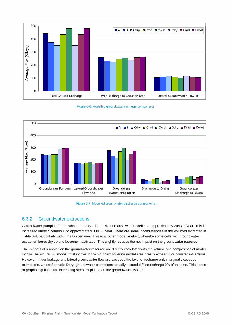
0

100

200

300

400

500

Total Diffuse Recharge River Recharge to Groundw ater Lateral Groundw ater Flow In

Ave

rage

Flu

x (G

L/yr

) .

A B Cdry Cmid Cw et Ddry Dmid Dw et

Figure 6-6. Modelled groundwater recharge components

0

100

200

300

400

500

Groundw ater Pumping Lateral Groundw aterFlow Out

Groundw aterEvapotranspiration

Discharge to Drains Groundw aterDischarge to Rivers

Ave

rage

Flu

x (G

L/yr

) .


Figure 6-7. Modelled groundwater discharge components

6.3.2 Groundwater extractions Groundwater pumping for the whole of the Southern Riverine area was modelled at approximately 245 GL/year. This is

increased under Scenario D to approximately 300 GL/year. There are some inconsistencies in the volumes extracted in

Table 6-4, particularly within the D scenarios. This is another model artefact, whereby some cells with groundwater

extraction bores dry up and become inactivated. This slightly reduces the net impact on the groundwater resource.

The impacts of pumping on the groundwater resource are directly correlated with the volume and composition of model

inflows. As Figure 6-8 shows, total inflows in the Southern Riverine model area greatly exceed groundwater extractions.

However if river leakage and lateral groundwater flow are excluded the level of recharge only marginally exceeds

extractions. Under Scenario Ddry, groundwater extractions actually exceed diffuse recharge 9% of the time. This series

of graphs highlights the increasing stresses placed on the groundwater system.


Table 6-4. Southern Riverine recharge compared to pumping under all scenarios

Volumes Without development


GL/y


River-derived recharge 224.2 260.1 230.2 225.5 246.3 254.4 237.6 257.0 264.0


percent

Time pumping exceeds total recharge 0% 0% 0% 0% 0% 9% 0% 0% 0%

Time pumping exceeds diffuse recharge 0% 0% 0% 0% 0% 9% 0% 0% 0%

0

250

500

750

1000

1250

1500

1750

1895 1905 1915 1925 1935 1945 1955 1965 1975 1985 1995 2005

Net

Flu

x (G

L/yr

)

Total Recharge - Scn A

Total Diffuse Recharge - Scn A

Total Diffuse Recharge - Scn Ddry

Groundw ater Extractions - Scn A

Figure 6-8. Comparison of recharge and groundwater extractions highlighting the increasing stresses on the resource

6.4 Groundwater indicators

Definitions of each of the groundwater resource condition indicators are provided in Table 6-5. The results of the

groundwater indicator assessment are presented in Table 6-6.

The 100% groundwater security across all scenarios suggests that from a purely resource-based perspective there is

little risk of long-term aquifer depletion. However the environmental indicator shows there is increasing risk

environmental impacts with a drier climate. This risk would be further enhanced if groundwater extractions were to

increase as under the D scenarios.

Table 6-5. Definition of groundwater indicators

Groundwater indicators

Groundwater security Percentage of years in which extraction is less than the average recharge over the previous ten-year period. Values less than 100 indicate increasing risk of sustained long-term groundwater depletion and thus a lower security of the groundwater resource.

Environmental groundwater indicator Ratio of average annual extraction to average annual recharge. Values of more than 1.00 indicate a long-term depletion of the groundwater resource and consequential long-term environmental impacts.

Groundwater drought indicator Difference in groundwater level (in metres) between the lowest level during each 111-year scenario simulation and the mean level under the baseline scenario. This is a relative indicator of the maximum drawdown under each scenario.


Table 6-6. Groundwater indicators under scenarios A, B, C and D


Groundwater security (%) 100% 100% 100% 100% 100% 100% 100% 100%

Environmental groundwater indicator (E/R) * 0.30 0.34 0.35 0.31 0.29 0.41 0.37 0.35

Groundwater drought indicator ** -1.40 -2.09 -2.46 -1.41 -0.95 -3.60 -2.42 -1.86

* E/R – Extractions / Recharge.

** Change from baseline (m) average for all bores.


7 Results by groundwater management unit


7.1 Campaspe Deep Lead WSPA

The Campaspe Deep Lead WSPA specifically applies to only the Calivil Formation and Renmark Group aquifers and

consequently river interactions are confined to very small areas where the Campaspe River bed intersects the Calivil

Formation in the south of the WSPA. The groundwater balance for the WSPA is presented in Table 7-1 and is also

supported by Figure 7-1 and Figure 7-2. Movement of water is constrained almost solely to flow across GMU boundaries,

as there is minimal direct interaction with rivers. However groundwater pumping is the largest discharge mechanism in

the water balance. Note that the inflows and outflows from ‘head-dependent boundaries’ represent interactions with the

surrounding and underlying bedrock aquifers.

Figure 7-3 highlights the direct impacts of groundwater pumping by comparing net flux under the without-development

scenario and Scenario A. These results indicate that the 26.5 GL/year of pumping is accounted for by approximately a 5

GL/year increase in leakage from the overlying Shepparton Formation and a ~21 GL/year increase in inflows from

surrounding aquifers (including the bedrock).

Table 7-1. Groundwater balance for the Campaspe Deep Lead WSPA



GL/y

Inflows (gains)


Head-dependent boundary 14.3 21.4 22.7 23.1 21.6 20.9 23.5 22.0 21.2


Leakage from overlying aquifer 13.0 17.8 16.6 16.3 17.6 18.3 14.9 16.4 17.3

Groundwater flow from adjacent zone

11.3 16.4 15.2 14.5 16.3 17.0 13.9 15.7 16.4

Total inflows 38.9 55.9 54.6 54.0 55.8 56.5 52.4 54.4 55.2

Outflows (losses)


Head-dependent boundaries 11.8 10.7 10.4 10.3 10.7 10.8 10.2 10.5 10.7

Leakage to overlying aquifer 0.1 0.7 0.8 0.8 0.7 0.7 0.8 0.7 0.6

Groundwater flow to adjacent zone

25.2 16.6 15.5 15.0 16.5 17.1 14.3 16.0 16.8

Groundwater discharge to rivers

1.8 1.3 1.5 1.4 1.3 1.3 1.4 1.3 1.3

Total outflows 38.9 55.8 54.7 54.0 55.7 56.4 52.5 54.3 55.2


0

10

20

30

40

50

Total Diffuse Recharge Head DependentBoundary

River Recharge toGroundw ater

Leakage fromOverlying Aquifer

GW Flow fromAdjacent Zone

Ave

rage

Flu

x (G

L/y

r) .


Figure 7-1. Groundwater inflows into the Campaspe Deep Lead WSPA

0

10

20

30

40

50

Groundw ater Pumping Head DependentBoundaries

Leakage to OverlyingAquifer

GW Flow to AdjacentZone

Groundw aterDischarge to Rivers

Ave

rag

e F

lux

(GL

/yr)

.


Figure 7-2. Groundwater outflows from the Campaspe Deep Lead WSPA

Figure 7-3. Impacts of groundwater pumping in the Campaspe Deep Lead WSPA


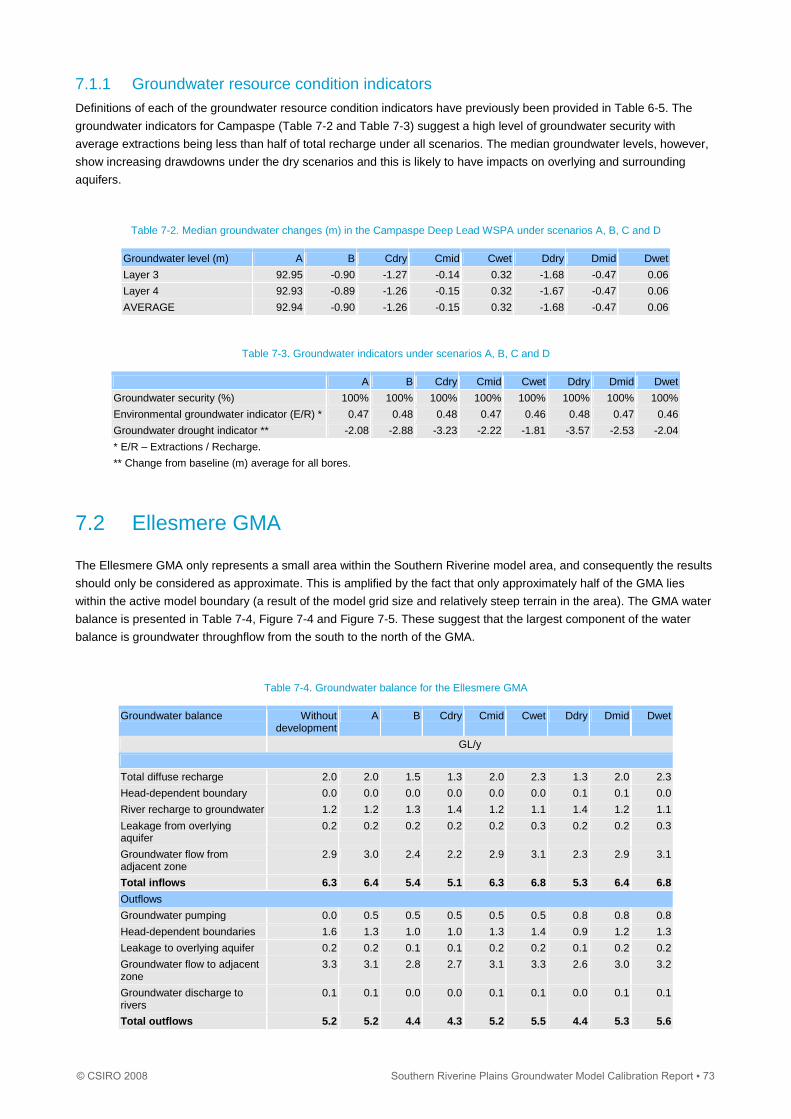
7.1.1 Groundwater resource condition indicators Definitions of each of the groundwater resource condition indicators have previously been provided in Table 6-5. The

groundwater indicators for Campaspe (Table 7-2 and Table 7-3) suggest a high level of groundwater security with

average extractions being less than half of total recharge under all scenarios. The median groundwater levels, however,

show increasing drawdowns under the dry scenarios and this is likely to have impacts on overlying and surrounding

aquifers.

Table 7-2. Median groundwater changes (m) in the Campaspe Deep Lead WSPA under scenarios A, B, C and D

Groundwater level (m) A B Cdry Cmid Cwet Ddry Dmid Dwet

Layer 3 92.95 -0.90 -1.27 -0.14 0.32 -1.68 -0.47 0.06

Layer 4 92.93 -0.89 -1.26 -0.15 0.32 -1.67 -0.47 0.06

AVERAGE 92.94 -0.90 -1.26 -0.15 0.32 -1.68 -0.47 0.06








7.2 Ellesmere GMA

The Ellesmere GMA only represents a small area within the Southern Riverine model area, and consequently the results

should only be considered as approximate. This is amplified by the fact that only approximately half of the GMA lies

within the active model boundary (a result of the model grid size and relatively steep terrain in the area). The GMA water

balance is presented in Table 7-4, Figure 7-4 and Figure 7-5. These suggest that the largest component of the water

balance is groundwater throughflow from the south to the north of the GMA.

Table 7-4. Groundwater balance for the Ellesmere GMA



GL/y




Leakage from overlying aquifer

0.2 0.2 0.2 0.2 0.2 0.3 0.2 0.2 0.3


2.9 3.0 2.4 2.2 2.9 3.1 2.3 2.9 3.1

Total inflows 6.3 6.4 5.4 5.1 6.3 6.8 5.3 6.4 6.8

Outflows





3.3 3.1 2.8 2.7 3.1 3.3 2.6 3.0 3.2


0.1 0.1 0.0 0.0 0.1 0.1 0.0 0.1 0.1

Total outflows 5.2 5.2 4.4 4.3 5.2 5.5 4.4 5.3 5.6


0

1

2

3

4

5





Ave

rage

Flu

x (G

L/yr

) .


Figure 7-4. Groundwater inflows into the Ellesmere GMA

0

1

2

3

4

5





Ave

rage

Flu

x (G

L/yr

) .


Figure 7-5. Groundwater outflows from the Ellesmere GMA


groundwater indicators for the Ellesmere GMA suggest a very high level of groundwater security (Table 7-5 and Table

7-6). However, given the coarse representation of the smaller GMUs, results may be skewed.

Table 7-5. Median groundwater changes (m) in the Ellesmere GMA under scenarios A, B, C and D


Average 133.33 -1.85 -2.51 -0.22 1.00 -2.56 -0.27 0.96

Layer 2 145.04 -4.76 -6.47 -0.57 2.63 -6.51 -0.62 2.59

Layer 3 127.58 -0.42 -0.56 -0.05 0.19 -0.61 -0.10 0.15

Layer 4 127.38 -0.38 -0.51 -0.04 0.18 -0.56 -0.08 0.14









7.3 Goorambat GMA

The Goorambat GMA represents a small area of the entire model and consequently the following water balance results

should only be considered as a guide. Within this modelling framework the impacts of climate on the water balance are

pronounced, with significant reductions in recharge under the dry scenarios and consequential increases in net river loss

(Table 7-7, Figure 7-6 and Figure 7-7).

Table 7-7. Groundwater balance for the Goorambat GMA



GL/y

Inflows





0.1 0.1 0.1 0.1 0.1 0.1 0.1 0.1 0.1

Total inflows 2.4 2.6 2.3 2.3 2.6 2.8 2.4 2.7 2.9

Outflows




0.9 0.9 0.9 0.9 0.9 1.0 0.9 0.9 1.0


0.5 0.4 0.3 0.2 0.4 0.5 0.2 0.4 0.4

Total outflows 1.4 1.6 1.5 1.4 1.6 1.8 1.5 1.7 1.8

0

1

2

3

4

5

Total Diffuse Recharge Head Dependent Boundary River Recharge toGroundw ater

GW Flow from AdjacentZone

Ave

rage

Flu

x (G

L/yr

) .


Figure 7-6. Groundwater inflows into the Goorambat GMA

0

1

2

3

4

5

Groundw ater Pumping Head Dependent Boundaries GW Flow to Adjacent Zone Groundw ater Discharge toRivers

Ave

rage

Flu

x (G

L/yr

) .


Figure 7-7. Groundwater outflows from the Goorambat GMA


7.3.1 Groundwater resource condition indicators Definitions of each of the groundwater resource condition indicators have previously been provided in Table 6-5.

Similarly to the Ellesmere GMA, the resource indicators for the Goorambat GMA may be skewed owing to the coarse

representation of the smaller GMUs.

Table 7-8. Median groundwater changes (m) in the Goorambat GMU under scenarios A, B, C and D


Layer 1 152.47 -0.14 -0.18 -0.02 0.06 -0.34 -0.17 -0.08

Layer 2 152.47 -0.15 -0.19 -0.02 0.06 -0.37 -0.19 -0.10

AVERAGE 152.47 -0.15 -0.19 -0.02 0.06 -0.35 -0.18 -0.09








7.4 Katunga WSPA

The Katunga WSPA lies within the centre of the Southern Riverine Plains model area and refers solely to the Deep Lead

aquifers. The Katunga WSPA has a simple mass balance, with the only recharge mechanism being inflows from

surrounding aquifers (including the overlying Shepparton WSPA). The only discharge mechanisms are groundwater

pumping and outflows across the GMU boundary (Table 7-10, Figure 7-8 and Figure 7-9).

Figure 7-10 highlights the impact of pumping within the WSPA, with approximate half of the volume pumped being

sourced from leakage from the overlying Shepparton Formation, and the remaining half being sourced from adjacent

aquifers. This result highlights the fact that pumping from the deep aquifer does cause drawdown of the watertable

aquifer and hence will impact on stream–aquifer interactions and may impact on GDEs.

Table 7-10. Groundwater balance for the Katunga WSPA



GL/y

Inflows



River recharge to groundwater

0.0 0.0 0.0 0.0 0.0 0.0 0.0 0.0 0.0

Leakage from overlying aquifer

8.0 18.5 18.5 18.5 18.5 18.6 17.0 16.8 16.9


20.7 35.2 35.2 35.3 35.2 35.2 34.5 34.7 34.7

Total inflows 28.7 53.7 53.7 53.8 53.7 53.8 51.5 51.5 51.6

Outflows





28.4 31.1 31.2 31.3 31.1 31.2 30.6 30.5 30.6


0.0 0.0 0.0 0.0 0.0 0.0 0.0 0.0 0.0

Total outflows 28.7 53.8 53.9 54.0 53.8 53.9 51.7 51.6 51.7


0

10

20

30

40

50

60

70





Ave

rage

Flu

x (G

L/y

r) .


Figure 7-8. Groundwater inflows into the Katunga WSPA

0

10

20

30

40

50

60

70





Ave

rage

Flu

x (G

L/yr

) .


Figure 7-9. Groundwater outflows from the Katunga WSPA

Figure 7-10. Impacts of groundwater pumping in the Katunga WSPA


7.4.1 Groundwater resource condition indicators Definitions of each of the groundwater resource condition indicators have previously been provided in Table 6-5. In

Katunga there is a slight reduction in groundwater pumping under Scenario D and consequently the environmental

indicator slightly reduces. As a result the most notable pattern in the resource condition indicators is the reduction in

median groundwater levels under the dry scenarios and Scenario B. There is also greater drawdown under the D

scenarios owing to increased extractions in surrounding GMUs and the overlying Shepparton WSPA.

Table 7-11. Median groundwater changes (m) in the Katunga WSPA under scenarios A, B, C and D


Layer 3 85.12 -1.02 -1.42 -0.18 0.30 -1.79 -0.50 0.05

Layer 4 84.81 -1.01 -1.41 -0.17 0.30 -1.73 -0.46 0.08

Average 84.98 -1.02 -1.42 -0.18 0.30 -1.76 -0.48 0.06








7.5 Kialla GMA

Despite only representing a minor component of the total model water balance the results for Kialla GMA hold some

important messages regarding interactions between GMUs. The water balance is almost entirely composed of

interactions with surrounding GMUs (Table 7-13, Figure 7-11 and Figure 7-12). When further analysed this is

predominantly composed of recharge via leakage from the overlying Shepparton WSPA and discharge to the Katunga

WSPA (to the north) and toward the Campaspe WSPA (to the west). Only very small volumes are pumped from the

Kialla GMA.

Figure 7-13 shows a comparison between the without-development scenario and Scenario A and indicates that leakage

from the Shepparton Formation increases by 8 GL/year to compensate for increased discharges through lateral

boundaries. In real terms this represents the spreading of the drawdown cones from pumping in the Katunga and

Campaspe WSPAs (and possibly further north in New South Wales).

As previously stated, in other GMUs increased leakage from the Shepparton Formation will have follow-on

consequences for stream–aquifer interactions and GDEs. This result again highlights the importance of accounting for

the impacts of groundwater pumping outside the GMU boundaries.


Table 7-13. Groundwater balance for the Kialla GMA



GL/y

Inflows





Groundwater flow from adjacent zone 6.2 6.6 6.6 6.6 6.6 6.6 6.6 6.6 6.5

Total inflows 15.5 23.0 23.0 23.1 22.9 22.9 23.1 22.9 22.8

Outflows




Groundwater flow to adjacent zone 14.5 22.5 22.5 22.7 22.5 22.5 22.7 22.4 22.3


Total outflows 15.6 23.0 23.0 23.2 23.0 23.0 23.2 22.9 22.8

0

5

10

15

20

25

30





Ave

rage

Flu

x (G

L/yr

) .


Figure 7-11. Groundwater inflows into the Kialla GMA

0

5

10

15

20

25

30





Ave

rage

Flu

x (G

L/yr

) .


Figure 7-12. Groundwater outflows from the Kialla GMA


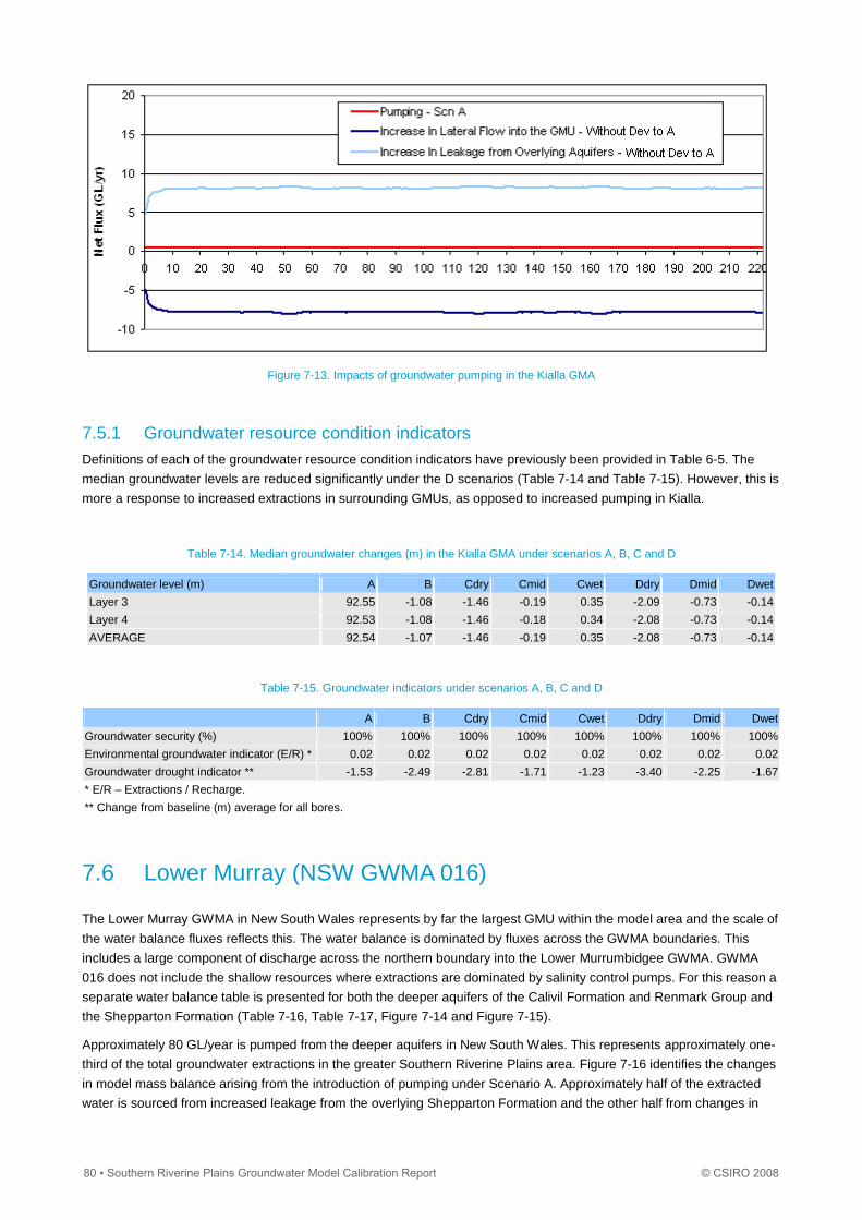
Figure 7-13. Impacts of groundwater pumping in the Kialla GMA


median groundwater levels are reduced significantly under the D scenarios (Table 7-14 and Table 7-15). However, this is

more a response to increased extractions in surrounding GMUs, as opposed to increased pumping in Kialla.

Table 7-14. Median groundwater changes (m) in the Kialla GMA under scenarios A, B, C and D


Layer 3 92.55 -1.08 -1.46 -0.19 0.35 -2.09 -0.73 -0.14

Layer 4 92.53 -1.08 -1.46 -0.18 0.34 -2.08 -0.73 -0.14

AVERAGE 92.54 -1.07 -1.46 -0.19 0.35 -2.08 -0.73 -0.14








7.6 Lower Murray (NSW GWMA 016)

The Lower Murray GWMA in New South Wales represents by far the largest GMU within the model area and the scale of

the water balance fluxes reflects this. The water balance is dominated by fluxes across the GWMA boundaries. This

includes a large component of discharge across the northern boundary into the Lower Murrumbidgee GWMA. GWMA

016 does not include the shallow resources where extractions are dominated by salinity control pumps. For this reason a

separate water balance table is presented for both the deeper aquifers of the Calivil Formation and Renmark Group and

the Shepparton Formation (Table 7-16, Table 7-17, Figure 7-14 and Figure 7-15).

Approximately 80 GL/year is pumped from the deeper aquifers in New South Wales. This represents approximately one-

third of the total groundwater extractions in the greater Southern Riverine Plains area. Figure 7-16 identifies the changes

in model mass balance arising from the introduction of pumping under Scenario A. Approximately half of the extracted

water is sourced from increased leakage from the overlying Shepparton Formation and the other half from changes in


flux across lateral boundaries. The water sourced from changes in lateral boundary fluxes is mostly through a reduced

net flow across the northern model boundary (i.e. reducing the water availability in the Lower Murrumbidgee GWMA).

The impacts of the increased leakage from the Shepparton to the Calivil Formation are also important. This causes

drawdown of the watertable and consequently increases river losses. However it is also noted that shallow watertables

caused by irrigation (and subsequent salinisation) have been a problem in this area.

Table 7-16. Groundwater balance for the Lower Murray GWMA 016 – Calivil Formation and Renmark Group



GL/y

Inflows






137.7 133.8 131.4 130.5 133.3 134.5 128.1 131.3 132.8

Total inflows 260.7 304.1 295.9 292.5 302.0 306.2 290.8 300.7 305.1

Outflows






Total outflows 260.2 303.7 295.6 292.2 301.7 305.9 290.5 300.4 304.7

Table 7-17. Groundwater balance for the Lower Murray GWMA 016 – Shepparton Formation



GL/y

Inflows




Upward leakage from underlying aquifer 44.5 40.0 38.4 37.9 39.6 40.3 37.3 39.1 39.9


Total inflows 261.6 274.1 245.2 233.9 266.8 284.2 232.8 266.2 283.7

Outflows



Leakage to underlying aquifer 74.9 108.8 100.6 96.8 106.6 110.8 97.2 107.0 111.2





Total outflows 252.0 267.6 240.4 229.2 260.7 277.2 228.4 260.1 276.7


0

50

100

150

200

250

300

Total DiffuseRecharge

Head DependentBoundary




Ave

rage

Flu

x (G

L/y

r) .


Figure 7-14. Groundwater inflows into the Lower Murray GWMA 016 – Calivil Formation and Renmark Group Aquifers

0

50

100

150

200

250

300





Ave

rage

Flu

x (G

L/yr

) .


Figure 7-15. Groundwater outflows from the Lower Murray GWMA 016 – Calivil Formation and Renmark Group Aquifers

Figure 7-16. Impacts of groundwater pumping in the Lower Murray GWMA 016 – Calivil Formation and Renmark Group Aquifers


7.6.1 Groundwater resource condition indicators Definitions of each of the groundwater resource condition indicators have previously been provided in Table 6-5. Due to

the high levels of irrigation recharge across the Lower Murray GWMA the levels of groundwater security and the median

groundwater level changes presented in Table 7-18 and Table 7-19 are relatively minor. The previous discussions on the

water balance present a greater analysis of the state of water resources in the Lower Murray GWMA.

Table 7-18. Median groundwater changes (m) in the Lower Murray groundwater management unit for baseline, recent and future

scenarios

Groundwater Level (m) A B Cdry Cmid Cwet Ddry Dmid Dwet

Layer 1 79.21 -0.80 -1.10 -0.13 0.28 -1.19 -0.20 0.23

Layer 2 78.03 -0.68 -0.95 -0.11 0.24 -1.06 -0.19 0.18

Layer 3 77.36 -0.56 -0.15 -0.09 0.20 -0.91 -0.18 0.13

Layer 4 77.35 -0.35 -0.80 -0.09 0.20 -0.91 -0.18 0.13

Average 77.99 -0.60 -0.75 -0.11 0.23 -1.02 -0.19 0.17

Table 7-19. Groundwater indicators for baseline, recent and future scenarios



Environmental Groundwater Indicator (E/R) * Shepparton Formation

0.08 0.09 0.09 0.08 0.08 0.09 0.08 0.08

Environmental Groundwater Indicator (E/R) * Deep Lead Aquifer

0.25 0.25 0.26 0.25 0.24 0.26 0.25 0.25

Groundwater Drought Indicator ** -0.80 0.88 -1.48 -0.91 -0.61 -1.74 -0.99 -0.67

* E/R – Extractions / Recharge

** Change from baseline (m) average for all bores

7.7 Mid-Goulburn GMA

Similar to the Campaspe WSPA, the Mid-Goulburn GMA refers to the Deep Lead aquifers and its water balance is

dominated by fluxes across the GMA boundaries (Table 7-20, Figure 7-17 and Figure 7-18). There are also small

volumes of direct rainfall recharge in the southern highlands where the Calivil Formation outcrops around the MDB

margins.

Given the GMA lies near the southern boundary of the MDB, and is enclosed largely by outcropping bedrock, the

majority of recharge occurs as leakage form the overlying Shepparton Formation. This is reflected in Figure 7-19 where

almost all the groundwater pumping in the GMA is accounted for by increased leakage from the Shepparton Formation.

This in turn is likely to have a strong influence on surface water flows in the Goulburn River catchment.


Table 7-20. Groundwater balance for the Mid-Goulburn GMA



GL/y

Inflows






0.0 0.0 0.0 0.0 0.0 0.0 0.0 0.0 0.0

Total inflows 7.7 8.6 8.0 8.0 8.5 8.9 8.9 9.2 9.6

Outflows





1.2 1.8 1.9 1.9 1.9 1.8 2.1 1.9 1.8


Total outflows 7.8 8.6 8.0 7.9 8.6 8.9 8.8 9.1 9.5

0

3

6

9

12

15





Ave

rage

Flu

x (G

L/y

r) .


Figure 7-17. Groundwater inflows into the Mid-Goulburn GMA

0

3

6

9

12

15





Ave

rage

Flu

x (G

L/yr

) .


Figure 7-18. Groundwater outflows from the Mid-Goulburn GMA


Figure 7-19. Impacts of groundwater pumping in the Mid-Goulburn GMA

7.7.1 Groundwater resource condition indicators Definitions of each of the groundwater resource condition indicators have previously been provided in Table 6-5. Bores in

the Mid-Goulburn GMA only screen the Calivil Formation therefore only one set of median groundwater levels is

presented in Table 7-21. These suggest quite significant drawdowns under Scenario Ddry, approximately 1.3 m across

the GMA. Table 7-22 also suggests an increase in the potential environmental stress under Scenario D.

Table 7-21. Median groundwater changes (m) in the Mid-Goulburn GMA under scenarios A, B, C and D


Average 113.18 -0.61 -0.81 -0.09 0.21 -2.09 -1.11 -0.74








7.8 Mid-Loddon GMA

The water balance presented here for the Mid-Loddon GMA, in Table 7-23 and diagrammatically in Figure 7-20 and

Figure 7-21, refers to all aquifers including the Shepparton Formation. Rainfall recharge is the dominant recharge

mechanism and consequently the impacts of climate variability are quite pronounced (~28 GL/year under the wet

scenarios and ~17 GL/year under the dry scenarios).

A comparison of the without-development scenario and Scenario A indicates that groundwater pumped from the GMA is

accounted for by increased river losses (32%), decreased groundwater evapotranspiration (34%), and decreased

groundwater flows out of the GMU (34%).


Table 7-23. Groundwater balance for the Mid-Loddon GMA



GL/y

Inflows





2.3 3.3 3.3 3.4 3.3 3.2 3.5 3.4 3.4

Total inflows 30.8 34.6 29.4 27.9 33.8 36.9 28.1 34.2 37.4

Outflows







Total outflows 30.7 34.5 29.5 27.8 33.8 37.0 28.1 34.3 37.5

0

10

20

30

40

50



Ave

rage

Flu

x (G

L/y

r) .


Figure 7-20. Groundwater inflows into the Mid-Loddon GMA

0

10

20

30

40

50

Groundw aterPumping

Head DependentBoundaries

GW Flow toAdjacent Zone


Discharge toDrains

Groundw aterDischarge to

Rivers

Ave

rage

Flu

x (G

L/yr

) .


Figure 7-21. Groundwater outflows from the Mid-Loddon GMA


7.8.1 Groundwater resource condition indicators Definitions of each of the groundwater resource condition indicators have previously been provided in Table 6-5. Given

there is very little difference in the volume of pumping between the scenarios the variations in the indicators are caused

largely by the climate (Table 7-24 and Table 7-25). In particular there are significant drawdowns in the Deep Lead

(~4.5 m) under the dry scenarios.

Table 7-24. Median groundwater changes (m) in the Mid-Loddon GMU under scenarios A, B, C and D


Layer 1 122.66 -1.26 -1.89 -0.16 0.53 -2.20 -0.39 0.31

Layer 2 120.54 -2.20 -3.54 -0.38 1.29 -3.70 -0.96 0.76

Layer 3 102.66 -2.66 -4.36 -0.46 1.64 -4.62 -1.24 0.84

Average 115.69 -2.05 -3.29 -0.34 1.16 -3.52 -0.87 0.64








7.9 Shepparton WSPA

The Shepparton WSPA refers to the shallow aquifers of the Shepparton Formation, overlying the Katunga WSPA, and

parts of the Campaspe WSPA, Kialla GMA and Mid-Goulburn GMA. The water balance of the WSPA is characterised by

large volumes of diffuse recharge (mainly from irrigation) and high levels of groundwater pumping, mostly for the control

of shallow watertables (Table 7-26, Figure 7-22 and Figure 7-23).

Despite the high levels of groundwater pumping in the WSPA, a comparison of the without-development scenario and

Scenario A shows an increase in groundwater flowing out of the WSPA when pumping is introduced. This can be

attributed to the high levels of pumping in the surrounding GMUs (most notably the Katunga WSPA, Campaspe WSPA

and Lower Murray GWMA). However it is also noted that the high levels of irrigation remain in the without-development

scenario. Hence without the extractions, large irrigation-induced groundwater mounds are likely to occur. There is also a

decrease in groundwater evapotranspiration because of groundwater pumping under Scenario A as a consequence of

the large reduction in area of shallow watertables. Reduction in evapotranspiration accounts for approximately 71% (50

GL/year) of the pumping. Such a reduction is likely to have a significant impact on GDEs such as the Barmah State

Forest.


Table 7-26. Groundwater balance for the Shepparton WSPA



GL/y

Inflows





17.4 16.2 15.4 14.9 16.0 16.5 14.8 16.1 16.6

Total inflows 258.6 268.1 237.4 228.9 261.3 277.7 240.4 271.4 286.7

Outflows







Total outflows 258.6 267.9 237.3 229.1 261.2 277.6 240.3 270.8 286.7

0

50

100

150

200

250



Ave

rage

Flu

x (G

L/y

r) .


Figure 7-22. Groundwater inflows into the Shepparton WSPA

0

50

100

150

200

250

Groundw aterPumping




Discharge toDrains


Rivers

Ave

rage

Flu

x (G

L/yr

) .


Figure 7-23. Groundwater outflows from the Shepparton WSPA


7.9.1 Groundwater resource condition indicators Definitions of each of the groundwater resource condition indicators have previously been provided in Table 6-5. There

are very large reductions in median groundwater levels under Scenario D as a result of increased extractions (Table

7-27). The increase in the environmental groundwater indicator from the A to the Cdry to the Ddry scenario highlights the

potential increasing stresses on the resource as a result of climate change and increasing extractions (Table 7-28).

Table 7-27. Median groundwater changes (m) in the Shepparton WSPA under scenarios A, B, C and D


Layer 1 102.34 -0.61 -0.87 -0.08 0.25 -7.16 -5.04 -4.28

Layer 2 96.82 -0.84 -1.19 -0.13 0.32 -3.27 -1.77 -1.74

Average 99.58 -0.12 -1.03 -0.10 0.28 -5.21 -3.40 -3.01






* E/R – Extractions / Recharge

** Change from baseline (m) average for all bores


8 Results by region


8.1 Campaspe

The model only covers a portion of the entire Campaspe region which extends well to the south beyond Bendigo. The

water balance results for the model area for the Campaspe region are presented in Table 8-1, Figure 8-1 and Figure 8-2.

The lower reaches of the region follow a thin strip along the Campaspe River and consequently lateral flows across the

region boundary represent a large portion of the water balance. The nature of the region boundary also produces an

artefact whereby the majority of pumping in the region is accounted for through increased groundwater flows across the

model boundaries (Table 8-2). These boundary fluxes significantly outweigh river interactions or changes in

evapotranspiration and represent a transfer of impacts from within the region to the surrounding areas where changes in

river exchange and evapotranspiration fluxes will occur.

Table 8-1. Groundwater balance for the Campaspe region



GL/y

Inflows





17.9 27.4 26.6 26.2 27.3 27.9 25.3 26.6 27.2

Total inflows 60.3 76.3 73.3 72.4 75.9 77.9 72.3 76.2 78.2

Outflows







Total outflows 60.3 76.4 73.4 72.3 75.9 77.9 72.4 76.2 78.2

Total river losses to groundwater -8.1 -4.7 -4.0 -3.2 -4.7 -5.7 -2.6 -3.8 -4.8

0

5

10

15

20

25

30

35

40



Ave

rage

Flu

x (G

L/y

r) .


Figure 8-1. Groundwater inflows into the Campaspe region


0

5

10

15

20

25

30

35

40

Groundw aterPumping




Discharge toDrains


Rivers

Ave

rage

Flu

x (G

L/yr

) .


Figure 8-2. Groundwater outflows from the Campaspe region

Table 8-2. Comparison of the without-development scenario and Scenario A in the Campaspe region

Groundwater balance Without development A Increase/decrease % of pumping

GL/y perecnt

Groundwater pumping 0.0 28.1 28.1 n/a

Total diffuse recharge 27.1 27.1 0.0 0%

Net flow in from head-dependent boundary

1.1 8.3 7.2 26%

Net flow in from adjacent zone -11.5 3.8 15.3 54%

Groundwater evapotranspiration -8.6 -6.5 2.1 7%

Net river loss to groundwater -8.1 -4.7 3.4 12%

Discharge to drains 0.0 0.0 0.0 0%

Net surface water losses -8.1 -4.7 3.4 12%

* Net surface water losses include both rivers and drains in the model.

8.2 Goulburn-Broken

The Southern Riverine groundwater model covers approximately the northern half of the Goulburn-Broken region. The

southern half is dominated by the outcropping bedrock formations of the Great Dividing Range and consequently have

limited groundwater availability.

The results of the Goulburn-Broken region highlight some of the complexities of regions that are not bounded by

hydrogeological boundaries. In particular Table 8-3 (supported by Figure 8-3, Figure 8-4 and Table 8-4) shows how the

lateral groundwater flow out of the region increases under scenarios with higher pumping. This results from the increases

in pumping in surrounding regions, specifically the enhanced drawdown cone centred near Deniliquin. In response to this,

there are large increases in net river loss and decreases in evapotranspiration. The result illustrates the importance of

considering the Southern River Plain as a single groundwater model and not as a number of discrete neighbouring

models. Had this area been developed as a standalone groundwater model it would have shown increased fluxes into

the model in response to long-term pumping. When considered in the correct setting of numerous productive aquifers

interacting within a continuum, the results illustrate the opposite (i.e. a reduction in fluxes into the area) due to greater

drawdown in neighbouring areas.

In this southern area the effects of climate change are pronounced, with significant reductions in rainfall recharge under

dry scenarios. This has significant follow on impacts for stream–aquifer interactions and evapotranspiration.


Table 8-3. Groundwater balance for the Goulburn-Broken region



GL/y

Inflows





36.8 32.6 32.0 31.7 32.5 32.9 30.7 31.2 31.5

Total inflows 193.4 195.4 171.6 166.3 190.0 201.9 177.3 198.3 209.2

Outflows







Total outflows 193.3 195.3 171.7 166.4 190.0 201.6 177.6 198.3 209.0


0

25

50

75

100

125



Ave

rage

Flu

x (G

L/y

r) .


Figure 8-3. Groundwater inflows into the Goulburn-Broken region

0

25

50

75

100

125

Groundw aterPumping




Discharge toDrains


Rivers

Ave

rage

Flu

x (G

L/yr

) .


Figure 8-4. Groundwater outflows from the Goulburn-Broken region


Table 8-4. Comparison of the without-development scenario and Scenario A in the Goulburn-Broken region


GL/y percent


Total diffuse recharge 111.0 110.8 -0.2 -1%


-3.1 -2.2 0.9 4%

Net flow in from adjacent zone -19.6 -37.7 -18.1 -73%


Net river loss to groundwater 14.8 29.4 14.6 59%

Discharge to drains -7.7 -4.0 3.7 15%

Net surface water losses 7.1 25.4 18.3 73%


8.3 Loddon-Avoca

Only the eastern half of the Loddon-Avoca region is covered by the groundwater model. This includes the Loddon River

but not the Avoca.

The results of the Loddon-Avoca region present a similar theme to that described in the Goulburn-Broken. In particular

Table 8-5 (supported by Figure 8-5, Figure 8-6 and Table 8-6) shows how the lateral groundwater flow out of the region

increases in scenarios with higher pumping. The increased outflows are caused by the increased pumping and greater

drawdown in surrounding regions. In response to this, there are large increases in net river loss and decreases in

evapotranspiration.

In this southern area the effects of climate change are pronounced, with significant reductions in rainfall recharge under

dry scenarios. This has significant follow-on impacts for stream–aquifer interactions and in particular evapotranspiration.

Evapotranspiration is particularly important in the Loddon due to large areas of shallow watertables, including a number

of saline lakes.

Table 8-5. Groundwater balance for the Loddon-Avoca region



GL/y

Inflows





Total inflows 126.2 131.6 116.2 111.6 129.5 139.5 112.4 130.2 140.3

Outflows







Total outflows 126.2 131.5 116.1 111.6 129.5 139.4 112.4 130.3 140.3



0

10

20

30

40

50

60

70

80

90

100



Ave

rage

Flu

x (G

L/y

r) .


Figure 8-5. Groundwater inflows into the Loddon-Avoca region

0

10

20

30

40

50

60

70

80

90

100

Groundw aterPumping




Discharge toDrains


Rivers

Ave

rage

Flu

x (G

L/yr

) .


Figure 8-6. Groundwater outflows from the Loddon-Avoca region

Table 8-6. Comparison of the without-development scenario and Scenario A in the Goulburn-Broken region


GL/y percent


Total diffuse fecharge 78.8 78.8 0.0 0%


8.4 14.5 6.1 32%

Net flow in from adjacent zone -43.6 -50.3 -6.7 -35%




Net surface water losses* 3.0 8.9 5.9 31%



8.4 Murray

The Murray region covers a large proportion of the model, including the area north of the Murray River (except in the

north-east where the model stretches into the Murrumbidgee region) and spanning some areas of Victoria including the

Katunga WSPA and the lower reaches of the Loddon River. It includes the entire length of the Murray River (within the

model domain) as well as the Wakool and Edward rivers.

The groundwater balance (presented in Table 8-7, Figure 8-7 and Figure 8-8) is comparable to that described in detail for

the entire model. A comparison of Scenario A with the without-development scenario (Table 8-8) suggests that 44% of

groundwater pumped from the region is derived from surface water sources, 30% via reduced groundwater

evapotranspiration, and the remainder (26%) from changes in lateral groundwater fluxes. These changes in lateral

groundwater fluxes are occurring across the northern boundary with the Murrumbidgee region and also across the

southern boundary where the region borders a number of Victorian regions. These results highlight the significant

potential for double accounting of water resources, with respect to both groundwater–surface water resources but also

groundwater resources in adjacent regions.

Table 8-7. Groundwater balance for the Murray region



GL/y





Total inflows 543.5 563.5 522.5 507.0 554.0 578.8 513.6 560.1 584.4







Total outflows 541.9 562.5 521.5 506.2 552.9 577.5 512.3 558.4 583.2


0

50

100

150

200

250

300



Ave

rage

Flu

x (G

L/y

r) .


Figure 8-7. Groundwater inflows into the Murray region


0

50

100

150

200

250

300

Groundw aterPumping




Discharge toDrains


Rivers

Ave

rage

Flu

x (G

L/yr

) .


Figure 8-8. Groundwater outflows from the Murray region

Table 8-8. Comparison of the without-development scenario and Scenario A in the Murray region


GL/y percent


Total diffuse recharge 197.8 197.8 0.0 0%


-75.1 -70.1 5.0 3%

Net flow in from adjacent zone 31.3 69.6 38.3 23%




Net surface water losses* 54.5 127.4 72.9 44%



9 Discussion of results

The results provided by the Southern Riverine groundwater model, within the context of the Murray-Darling Basin

Sustainable Yields Project, can be viewed as a significant stepping stone toward bridging some of the knowledge gaps in

integrated water resources management. A few of the key issues identified from the modelling are discussed below.

• Water accounting across GMU boundaries – The groundwater model is a regional model that encompasses

nine separate groundwater management areas and four regions defined in this project. This enabled some key

regional scale conclusions as follows:

o The results from the scenario modelling highlighted the significant levels of interaction that occur

between GMUs and regions. For example, the high levels of groundwater extractions in the Lower

Murray (NSW GWMA 016) were found to be drawing upon the groundwater resources from

neighbouring aquifers such as the Murrumbidgee to the north and Katunga to the south (approximately

50% of the volume pumped).

o Similarly, pumping in the Katunga and Shepparton WSPAs was found to be drawing large volumes of

water from aquifers to the south such as those found in the Kialla and Mid-Goulburn GMAs. This

occurred to the extent that in spite of increased extractions in Kialla, groundwater flow out of the GMA

increases because of pumping in neighbouring GMUs (as seen by comparing the without-development

scenario and Scenario A). A model constructed for the Kialla GMA alone would have presented the

opposite result, not reflecting the regional scale processes.

o The iterative calibration process also highlighted the extent of the drawdown cone centred near

Deniliquin. The area of influence from this drawdown cone is likely to extend as far as the Loddon

catchment in the west and into the Murrumbidgee in the north.

o Problems arose from the inability to accurately represent interactions to the north with the

Murrumbidgee. This highlights both the benefits of regional scale models, but also the limitations of

current groundwater models.

• Surface–groundwater interactions – The scale of the Southern Riverine model has the advantage of limiting

the influence of ‘artificial’ model boundaries. This results in an increased percentage of model inflows and

outflows sourced by real processes, such as changes in evapotranspiration and river leakage. This in turn

minimises the chances of large errors occurring in the water balance. By comparing scenarios with identical

climates but altered pumping regimes, the impacts of groundwater pumping on the rest of the water balance can

be understood.

o By comparing scenarios Cmid and Dmid where pumping is increased by ~50 GL/year, it was found

that 58% of this volume extracted was sourced from water that would have otherwise added to surface

water flows.

o The majority of the remainder of the water was sourced from groundwater evapotranspiration (37%)

with 5% from lateral flow across model boundaries. This very small volume sourced from model

boundaries suggests that the model is accounting for the regional scale impacts of groundwater

pumping.

The time lag associated with the impacts of groundwater pumping on streamflows varies on a scale from years

to several decades, depending on the depth and location of extraction wells. Under Scenario A the full impacts

of all groundwater extractions are observed within 25 years.

• Groundwater evapotranspiration – The importance of groundwater evapotranspiration was first highlighted

during the calibration process where it was discovered that groundwater evapotranspiration from forested areas

such as the Gunbower Forest significantly influenced the groundwater levels. Throughout the scenario

modelling process, evapotranspiration proved to be the most sensitive discharge mechanism in response to

climate change.

Under the dry scenarios, decreases in rainfall recharge were largely matched by decreases in groundwater

evapotranspiration. This is possibly realised by losses in water availability to groundwater-dependent

ecosystems. In practical terms, this suggests that unless water allocations are reduced in the future in


accordance with the reduced rainfall recharge, environmental assets are likely to incur the biggest losses as a

result of climate change.

• Without-development conditions – Under the without-development scenario the groundwater levels across

the model rise to levels above those modelled during the calibration period. Consequently it is emphasised that

the groundwater model is not calibrated for such conditions, and therefore the results should only be considered

approximate on a broad scale.

The elevated groundwater levels under the without-development scenario increase groundwater flow out of the

model region, increase discharges to surface water bodies, and increase evapotranspiration. With reference to

the current conditions, 42% of current groundwater pumping was estimated to be derived from surface water

bodies. However, this is considered to be an underestimate as 19% was sourced from lateral groundwater flow

and hence is likely to be an artefact of model boundary conditions.


10 Modelling limitations and recommendations

The large size and complexity of the Southern Riverine model provided many hurdles during the model construction,

calibration, and scenario modelling process. Some of the major hurdles and limitations are discussed below.

A 1 km grid cell resolution was built in to the model. In compliance with this resolution, the digital terrain model

approximates an average elevation across each 1 km grid cell. This resolution does not capture localised details such as

drainage lines causing a number of modelling issues.

The combination of the steep terrain in the south and the 1 km x 1 km grid cell resolution caused many modelling stability

problems. Across the great divide in the south there are many cases where elevation changes between adjacent grid

cells exceed 50 m. Such occurrences made it necessary to inactivate many areas where the steep terrain was causing

instability. Observed steep hydraulic gradients in the south also created problems for the calibration. This was particularly

the case along the upper reaches of the Goulburn River where attempts to force the model to replicate the observed

gradients lead to model non-convergence. This subsequently led to a sub-optimal calibration.

A secondary limitation was found during calibration when some observation bores were found to depict watertables

above the digital terrain model elevation. It is assumed that this arose from the digital terrain model not capturing the

necessary level of localised detail. Despite the problems caused by the grid cell resolution it is not considered that further

grid refinement would be advantageous. As explained below the computational requirements of a finer grid would more

than likely render the model unsuitable for most projects.

The computational speed of model runs was a consistent impediment throughout the project. Despite only being a

moderate complexity model, the model resolution, layering and data complexity lead to long run times. The inclusion of

over 2000 groundwater extraction wells in the model significantly slowed the model (approximately doubling the run time).

It was assumed that this was more related to the increased stresses placed on the aquifers. This, in turn, increases the

number of cells that dry out during model runs and further hinders model convergence.

The final calibration model took approximately 3 hours to complete the 16-year calibration period. This run time hinders

the ability to complete large numbers of iterations in an attempt to find an optimised solution. The use of automated

parameter estimation software (such as PEST) was deemed inappropriate given the very short time frame for this project.

Furthermore it is considered unlikely to aid any further calibration attempts due the high chance of model convergence

failures.

Each 111-year scenario required 10 to 15 hours to run to completion. The budget file generated from each run exceeded

20 GB, complicating and slowing post-processing procedures. The run times, file sizes and model complexity are a

significant limitation for potential future uses of the model.

Groundwater evapotranspiration is known to be a very important part of the water balance. In the area of Gunbower

Forest, the inclusion of evapotranspiration with a deep extinction depth and higher maximum rates proved to greatly

enhance the match of observed and simulated hydrographs within the forest. However the spatial variability of

groundwater evapotranspiration across the model domain is still poorly understood. The variability within the model has

evolved in a manner that suits model calibration as opposed to being based on scientific rationale. Further study of

evapotranspiration variability on a regional scale would reduce the level of uncertainty in the model water balance.

The majority of model boundaries coincide with hydrogeological boundaries such as the bedrock in the south. This is a

significant advantage and aids in the reduction of modelling uncertainty. However the northern boundary with the

Murrumbidgee catchment remains a potential source of error. A comparison of the fluxes across this boundary was

undertaken by interrogating both the Southern Riverine and Lower Murrumbidgee groundwater models. The comparison

showed both models were discharging water across the boundary. There are a number of possible explanations for the

apparent discrepancy:

• Firstly, it is possible that there is a component of real groundwater discharge into the Edward River and

Billabong Creek. However, it is likely that river discharge would only account for a small proportion of this flux.


• Secondly, in the Wakool Junction area to the west, there is overlap between the model areas and it is possible

that some of the modelled discharges are both to the west out of both model areas. This is supported by the

regional flow directions which approximately follow the surface water drainage lines.

• Finally there are discrepancies in the boundary conditions assigned to the common boundary between the

models. The Lower Murrumbidgee uses a constant head boundary along the entire length of Billabong Creek.

The Southern Riverine model specifies a no flow boundary in the eastern half of this boundary and a general

head boundary in the western half. The no flow boundary was specified for two reasons:

1. The direction of groundwater flow in this region is parallel to this boundary; hence minimal fluxes

occur across the boundary.

2. During calibration it was found that defining a boundary head and allowing water to cross this

boundary always induced too much flow toward the cone of depression from Deniliquin and

consequently drawdown levels were not being matched. Lowering the boundary head would

precondition the model to a stressed state and therefore was deemed inappropriate. Variable heads

are not considered appropriate for long-term scenario modelling. Consequently the most appropriate

solution was deemed to be a no flow boundary.

The grid cell size also creates problems for accurate modelling of surface–groundwater interaction. Local scale

features are hard to represent, particularly where the terrain becomes very steep such as in the southern extremes of the

Loddon, Goulburn and Broken rivers. In the upper reaches of the Goulburn and Broken many stretches of river appear to

be flanked by outcropping bedrock when considered on a 1 km grid resolution. This restricts the model’s ability to

simulate fluxes between the rivers and the surrounding aquifers.

Despite the above inaccuracies, the simulation of river–aquifer interactions on the plains is generally considered to be of

good quality. This includes the Murray River, Wakool River, Edward River and the lower reaches of the Loddon,

Campaspe, Goulburn and Broken rivers. This represents by far the bulk of the river–aquifer interactions across the model

domain. Therefore the fluxes reported are still considered to be meaningful results.

Simulation of without-development conditions has been used within this project to assess the impacts of current

groundwater usage in the model. However, it has already been acknowledged that such scenarios push the model

beyond its calibration and therefore the degree of uncertainty is increased. A factor of this is the decision to leave

irrigation recharge in the without-development scenario, which can lead to excessive recharge and irrigation-induced

groundwater mounding in shallow aquifers.

Unfortunately there is very little that can be done to reduce the uncertainty due to the lack of groundwater observations

prior to the development of the resource. However, the results of the without-development scenarios can still be

considered as a useful baseline against which the impacts of current development can be gauged.

Finally some of the greatest model improvements could be made as more accurate calibration model data becomes

available. Many of the data shortfalls have previously been mentioned throughout this report but the following points

summarise the key data requirements:

• Historical groundwater usage data proved to be unreliable. Metering has only occurred on a broad scale since

approximately 1999. However even after this time metered use does not include all production bores.

Throughout the calibration modelling there was significant evidence that current estimates of usage may be well

under actual historical usage. Further analysis and clarification of usage rates would greatly aid model

calibration.

• Surface water elevations also proved to be unreliable, with many gauge sites not having surveyed elevations,

and many others reporting different elevations from different sources. River elevations are obviously vital for

modelling of surface–groundwater interactions; therefore improvement of river elevation data should be

considered a priority.

• The digital terrain model was a further source of error where some surveyed bores suggested watertables

above the surface. An improved digital terrain model may aid any further model calibration attempts.


11 References

Bureau of Meteorology (2006) Australian Rainfall Districts Map. Australian Government – Bureau of Meteorology.

DIPNR (2004) Water Sharing Plan for the Murray and Lower Darling Regulated Rivers Water Sources. Department of Infrastructure, Planning and Natural Resources, NSW.

DLWC (2001) Groundwater Management Model for GWMA016 – Lower Murray Region. Volume 1 – Model Development and Calibration. Department of Land & water Conservation.

GMW (2006) Shepparton Irrigation Region WSPA Management Plan (Groundwater). Report for the year ended June 2006.

GMW (2006a) Groundwater Management Plan for the Katunga Water Supply Protection Area.

Hyder Consulting (2006) Campaspe Valley Conceptual Hydrogeological Model. Report for Goulburn Murray Water. May 2006.

Middlemis H (2000) Murray Darling Basin Commission Groundwater Flow Modelling Guidelines. Nov 2000.

MIL (2006) Murray Irrigation Limited Annual Report 2006. Murray Irrigation Limited. Deniliquin, NSW.

SKM (2003) Projections of Groundwater Extraction Rates and Implications for Future Demand and Competition for Surface Water. Report prepared for Murray Darling Basin Commission and CSIRO Australia. Canberra, ACT.

SKM (2006) Draft Mid-Goulburn GMA Conceptual Model. Report prepared for Goulburn Murray Water. June 2006.

URS (2006) Mid Loddon WSPA Groundwater Model – Stage 2 Conceptual Model Refinement. Report prepared for Goulburn Murray Water. June 2006.


12 Appendix A – River gauges

Gauge ID Gauge name Scenario model data source

404200 Broken River @ Goorambat (T. Gauge) REALM-GSM

404203 Broken River @ Benalla REALM-GSM

404210 Broken Creek @ Rices Weir Interpolated

404214 Broken Creek @ Katamatite Interpolated

404216 Broken River @ Goorambat (H. Gauge) REALM-GSM

404217 Broken Creek @ Casey Weir REALM-GSM

404222 Broken River @ Orrvale REALM-GSM

404224 Broken River @ Gowngardie REALM-GSM

404226 Broken River @ Lake Mokoan REALM-GSM

405200 Goulburn River @ Murchison REALM-GSM

405202 Goulburn River @ Seymour REALM-GSM

405204 Goulburn River @ Sheparton REALM-GSM

405232 Goulburn River @ McCoy Bridge REALM-GSM

405253 Goulburn River @ Goulburn Weir REALM-GSM

405259 Goulburn River @ Goulburn Weir REALM-GSM

406001 Campaspe River @ Site 1 REALM-GSM






406201 Campaspe River @ Barnadown REALM-GSM

406202 Campaspe River @ Rochester REALM-GSM

406265 Campaspe River @ Echuca MSM-BIGMOD

407200 Loddon River @ Bridgewater REALM-GSM

407203 Loddon River @ Laanecombe REALM-GSM

407205 Loddon River @ Appin South REALM-GSM

407210 Loddon River @ Cairn Curran Res REALM-GSM

407224 Loddon River @ Loddon Weir REALM-GSM

407229 Loddon River @ Serpentine Weir REALM-GSM

407240 Loddon River @ Laanecombe Res REALM-GSM

407243 Loddon River @ Loddon Weir (H. Gauge) REALM-GSM

409003 Edward River @ Deniliquin MSM-BIGMOD

409005 Murray River @ Barham MSM-BIGMOD

409008 Edward River @ Offtake MSM-BIGMOD

409013 Wakool River @ Stony Crossing MSM-BIGMOD

409014 Edward River @ Moulamein Interpolated

409019 Wakool River @ Offtake MSM-BIGMOD

409023 Edward River @ Stevens Weir MSM-BIGMOD

409025 Murray River @ D/S Yarrawonga Weir MSM-BIGMOD

409035 Edward River @ Liewah MSM-BIGMOD

409045 Wakool River @ Wakool Barham MSM-BIGMOD

409048 Neimur Creek @ Barham Rd Interpolated

409061 Wakool River @ Coonimit Bridge Interpolated

409202 Murray River @ Tocumwal MSM-BIGMOD

409204 Murray River @ Swan Hill MSM-BIGMOD

409207 Murray River @ Torrumbarry MSM-BIGMOD

409213 Murray River @ Piangil Interpolated

409215 Murray River @ Barmah MSM-BIGMOD

409216 Murray River @ Yarrawonga Weir MSM-BIGMOD

409217 Murray River @ Cobram Interpolated

409221 Murray River @ Lower Moira Interpolated

414200 Murray River @ Below Wakool Junction MSM-BIGMOD

409219 – “Gun1” Murray River @ Torrumbarry Weir MSM-BIGMOD


Gauge ID Gauge name Scenario model data source

“Gun2” Murray River @ D/S Torrumbarry Weir MSM-BIGMOD


13 Appendix B – Calibration model observation

bores

Bore ID Area LCC Easting LCC Northing Aquifer monitored

62595 Campaspe 873055 1438687 Calivil



60128 Campaspe 874329 1463189 Lower_Shep




47253 Campaspe 876761 1471737 Renmark







46190 Goul_Brok 943948 1438411 Calivil






46195 Goul_Brok 946195 1445754 Lower_Shep





56424 Goul_Brok 950865 1478318 Renmark

54409 Goul_Brok 963951 1450522 Upper_Shep








36154 Gunbower 838755 1532124 Lower_Shep

36083 Gunbower 841354 1525759 Renmark



36084 Gunbower 840824 1525229 Upper_Shep






105936 Katunga 930546 1513897 Calivil

111544 Katunga 993946 1501350 Calivil

48200 Katunga 931073 1494190 Calivil

48282 Katunga 949303 1497776 Calivil

53673 Katunga 989278 1503588 Calivil

53674 Katunga 988659 1498063 Calivil

92405 Katunga 949261 1514726 Calivil

97613 Katunga 940252 1502772 Calivil



109557 Katunga 968267 1499070 Lower_Shep

109680 Katunga 949389 1504180 Renmark

51001 Katunga 982371 1500159 Renmark

69545 Katunga 974135 1499808 Renmark

50325 Loddon 787712 1560815 Calivil

82760 Loddon 814011 1553172 Calivil

88214 Loddon 827601 1452384 Calivil

36415 Loddon 818306 1452302 Lower_Shep




50314 Loddon 790302 1547184 Renmark

82757 Loddon 813113 1542521 Renmark

82761 Loddon 813749 1553182 Renmark

138651 Loddon 813356 1392076 Upper_Shep








36102 NSW 840031 1565575 Calivil

36584 NSW 942527 1522160 Calivil

36585 NSW 927180 1540066 Calivil

36586 NSW 940435 1538353 Calivil

36588 NSW 922584 1528563 Calivil

36589 NSW 905687 1519396 Calivil

36742 NSW 917545 1556423 Calivil

36765 NSW 875299 1509772 Calivil

36772 NSW 833066 1544747 Calivil

36775 NSW 853703 1539093 Calivil

36824 NSW 799441 1595031 Calivil

36353 NSW 1026660 1502217 Lower_Shep

36356 NSW 996806 1505949 Lower_Shep

36557 NSW 834949 1572454 Lower_Shep

36744 NSW 949952 1553993 Lower_Shep

36747 NSW 877566 1536612 Lower_Shep

36823 NSW 816602 1572601 Lower_Shep

36283 NSW 950670 1528305 Renmark

36564 NSW 832399 1576094 Renmark

36587 NSW 913964 1542916 Renmark

36743 NSW 935655 1552740 Renmark

36766 NSW 879703 1556930 Renmark

36822 NSW 793101 1572753 Renmark

36871 NSW 866476 1580825 Renmark

36350 NSW 1009045 1514298 Shepparton

36351 NSW 1015555 1514002 Shepparton

36391 NSW 1014810 1520662 Shepparton

36394 NSW 1028582 1521276 Shepparton

36438 NSW 1016302 1531116 Upper_Shep

36635 NSW 984989 1567573 Upper_Shep

36636 NSW 986148 1553648 Upper_Shep

36639 NSW 994449 1555991 Upper_Shep

36644 NSW 890669 1497073 Upper_Shep

36718 NSW 766273 1611999 Upper_Shep

36821 NSW 779251 1593327 Upper_Shep

105701 Shepparton 904103 1485241 Lower_Shep







105702 Shepparton 903778 1485598 Upper_Shep





























14 Appendix C – Calibration model hydrographs

14.1 New South Wales

60

62

64

66

68

70

72

74

76

78

80

1990 1993 1996 1999 2002 2005

Red

uced

Wat

er L

evel

(m

AH

D)

36871 - Layer 4 (CAL)

36871 - Layer 4 (OBS)

36766 - Layer 4 (CAL)

36766 - Layer 4 (OBS)

80

82

84

86

88

90

92

94

96

98

100

1990 1993 1996 1999 2002 2005

Red

uced

Wat

er L

evel

(m

AH

D)

36639 - Layer 1 (CAL)36639 - Layer 1 (OBS)36636 - Layer 1 (CAL)36636 - Layer 1 (OBS)36635 - Layer 1 (CAL)36635 - Layer 1 (OBS)

95

97

99

101

103

105

107

109

111

113

115

1990 1993 1996 1999 2002 2005

Red

uced

Wat

er L

evel

(m

AH

D)

36438 - Layer 1 (CAL)

36438 - Layer 1 (OBS)

36394 - Layer 1 (CAL)

36394 - Layer 1 (OBS)


100

102

104

106

108

110

112

114

116

118

120

1990 1993 1996 1999 2002 2005

Red

uced

Wat

er L

evel

(m

AH

D)

36391 - Layer 1 (CAL)36391 - Layer 1 (OBS)36351 - Layer 1 (CAL)36351 - Layer 1 (OBS)36350 - Layer 1 (CAL)36350 - Layer 1 (OBS)

110

112

114

116

118

120

122

124

126

128

130

1990 1993 1996 1999 2002 2005

Red

uced

Wat

er L

evel

(m

AH

D)

36356 - Layer 2 (CAL)

36356 - Layer 2 (OBS)

36353 - Layer 2 (CAL)

36353 - Layer 2 (OBS)

65

70

75

80

85

90

95

1990 1993 1996 1999 2002 2005

Red

uced

Wat

er L

evel

(m

AH

D)

36744 - Layer 2 (CAL)36744 - Layer 2 (OBS)




65

70

75

80

85

90

95

1990 1993 1996 1999 2002 2005

Red

uced

Wat

er L

evel

(m

AH

D)

36587 - Layer 4 (CAL)

36587 - Layer 4 (OBS)

36586 - Layer 3 (CAL)

36586 - Layer 3 (OBS)

36585 - Layer 3 (CAL)

36585 - Layer 3 (OBS)

70

75

80

85

90

95

100

1990 1993 1996 1999 2002 2005

Red

uced

Wat

er L

evel

(m

AH

D)

36584 - Layer 3 (CAL)

36584 - Layer 3 (OBS)

36283 - Layer 4 (CAL)

36283 - Layer 4 (OBS)

70

72

74

76

78

80

82

84

86

88

90

1990 1993 1996 1999 2002 2005

Red

uced

Wat

er L

evel

(m

AH

D)

36589 - Layer 3 (CAL)

36589 - Layer 3 (OBS)

36588 - Layer 3 (CAL)

36588 - Layer 3 (OBS)


70

72

74

76

78

80

82

84

86

88

90

1990 1993 1996 1999 2002 2005

Red

uced

Wat

er L

evel

(m

AH

D)

36765 - Layer 3 (CAL)

36765 - Layer 3 (OBS)

36644 - Layer 1 (CAL)

36644 - Layer 1 (OBS)

65

67

69

71

73

75

77

79

81

83

85

1990 1993 1996 1999 2002 2005

Red

uced

Wat

er L

evel

(m

AH

D)




65

67

69

71

73

75

77

79

81

83

85

1990 1993 1996 1999 2002 2005

Red

uced

Wat

er L

evel

(m

AH

D)

36564 - Layer 4 (CAL)

36564 - Layer 4 (OBS)

36557 - Layer 2 (CAL)

36557 - Layer 2 (OBS)

36102 - Layer 3 (CAL)

36102 - Layer 3 (OBS)


55

57

59

61

63

65

67

69

71

73

75

1990 1993 1996 1999 2002 2005

Red

uced

Wat

er L

evel

(m

AH

D)

36824 - Layer 3 (CAL)

36824 - Layer 3 (OBS)

36822 - Layer 4 (CAL)

36822 - Layer 4 (OBS)

50

52

54

56

58

60

62

64

66

68

70

1990 1993 1996 1999 2002 2005

Red

uced

Wat

er L

evel

(m

AH

D)

36821 - Layer 1 (CAL)

36821 - Layer 1 (OBS)

36718 - Layer 1 (CAL)

36718 - Layer 1 (OBS)

14.2 Gunbower Forest

60

62

64

66

68

70

72

74

76

78

80

1990 1993 1996 1999 2002 2005

Red

uced

Wat

er L

evel

(m

AH

D)

36155 - Layer 1 (CAL)

36155 - Layer 1 (OBS)

36154 - Layer 2 (CAL)

36154 - Layer 2 (OBS)


60

62

64

66

68

70

72

74

76

78

80

1990 1993 1996 1999 2002 2005

Red

uced

Wat

er L

evel

(m

AH

D)




60

62

64

66

68

70

72

74

76

78

80

1990 1993 1996 1999 2002 2005

Red

uced

Wat

er L

evel

(m

AH

D)

36084 - Layer 1 (CAL)

36084 - Layer 1 (OBS)

36083 - Layer 4 (CAL)

36083 - Layer 4 (OBS)

60

62

64

66

68

70

72

74

76

78

80

1990 1993 1996 1999 2002 2005

Red

uced

Wat

er L

evel

(m

AH

D)

36162 - Layer 4 (CAL)

36162 - Layer 4 (OBS)

36161 - Layer 4 (CAL)

36161 - Layer 4 (OBS)


70

72

74

76

78

80

82

84

86

88

90

1990 1993 1996 1999 2002 2005

Red

uced

Wat

er L

evel

(m

AH

D)

36170 - Layer 1 (CAL)

36170 - Layer 1 (OBS)

70

72

74

76

78

80

82

84

86

88

90

1990 1993 1996 1999 2002 2005

Red

uced

Wat

er L

evel

(m

AH

D)

87809 - Layer 1 (CAL)

87809 - Layer 1 (OBS)

87808 - Layer 1 (CAL)

87808 - Layer 1 (OBS)

14.3 Loddon

60

62

64

66

68

70

72

74

76

78

80

1990 1993 1996 1999 2002 2005

Red

uced

Wat

er L

evel

(m

AH

D)

50328 - Layer 2 (CAL)

50328 - Layer 2 (OBS)

50325 - Layer 3 (OBS)

50325 - Layer 3 (CAL)


60

62

64

66

68

70

72

74

76

78

80

1990 1993 1996 1999 2002 2005

Red

uced

Wat

er L

evel

(m

AH

D)

50317 - Layer 1 (OBS)

50317 - Layer 1 (CAL)

50314 - Layer 4 (OBS)

50314 - Layer 4 (CAL)

60

62

64

66

68

70

72

74

76

78

80

1990 1993 1996 1999 2002 2005

Red

uced

Wat

er L

evel

(m

AH

D)

82759 - Layer 1 (CAL)

82759 - Layer 1 (OBS)

82758 - Layer 2 (CAL)

82758 - Layer 2 (OBS)

82757 - Layer 4 (CAL)

82757 - Layer 4 (OBS)

70

72

74

76

78

80

82

84

86

88

90

1990 1993 1996 1999 2002 2005

Red

uced

Wat

er L

evel

(m

AH

D)

76761 - Layer 1 (CAL)

76761 - Layer 1 (OBS)


90

92

94

96

98

100

102

104

106

108

110

1990 1993 1996 1999 2002 2005

Red

uced

Wat

er L

evel

(m

AH

D)

66868 - Layer 2 (CAL)

66868 - Layer 2 (OBS)

66867 - Layer 1 (CAL)

66867 - Layer 1 (OBS)

100

102

104

106

108

110

112

114

116

118

120

1990 1993 1996 1999 2002 2005

Red

uced

Wat

er L

evel

(m

AH

D)

67956 - Layer 1 (CAL)

67956 - Layer 1 (OBS)

100

102

104

106

108

110

112

114

116

118

120

1990 1993 1996 1999 2002 2005

Red

uced

Wat

er L

evel

(m

AH

D)

36416 - Layer 1 (OBS)

36416 - Layer 1 (CAL)

36415 - Layer 2 (OBS)

36415 - Layer 2 (CAL)


90

95

100

105

110

115

120

1990 1993 1996 1999 2002 2005

Red

uced

Wat

er L

evel

(m

AH

D)

88239 - Layer 1 (CAL)

88239 - Layer 1 (OBS)

88214 - Layer 3 (CAL)

88214 - Layer 3 (OBS)

170

172

174

176

178

180

182

184

186

188

190

1990 1993 1996 1999 2002 2005

Red

uced

Wat

er L

evel

(m

AH

D)

138651 - Layer 1 (OBS)

138651 - Layer 1 (CAL)

14.4 Campaspe

75

77

79

81

83

85

87

89

91

93

95

1990 1993 1996 1999 2002 2005

Red

uced

Wat

er L

evel

(m

AH

D)

95041 - Layer 3 (CAL)

95041 - Layer 3 (OBS)

95042 - Layer 1 (CAL)

95042 - Layer 1 (OBS)


90

92

94

96

98

100

102

104

106

108

110

1990 1993 1996 1999 2002 2005

Red

uced

Wat

er L

evel

(m

AH

D)

97120 - Layer 1 (CAL)

97120 - Layer 1 (OBS)

70

75

80

85

90

95

100

1990 1993 1996 1999 2002 2005

Red

uced

Wat

er L

evel

(m

AH

D)

79324 - Layer 4 (CAL)

79324 - Layer 4 (OBS)

79329 - Layer 1 (CAL)

79329 - Layer 1 (OBS)

75

77

79

81

83

85

87

89

91

93

95

1990 1993 1996 1999 2002 2005

Red

uced

Wat

er L

evel

(m

AH

D)

62036 - Layer 4 (CAL)

62036 - Layer 4 (OBS)

61957 - Layer 4 (CAL)

61957 - Layer 4 (OBS)


65

70

75

80

85

90

95

100

105

110

1990 1993 1996 1999 2002 2005

Red

uced

Wat

er L

evel

(m

AH

D)

47253 - Layer 4 (CAL)

47253 - Layer 4 (OBS)

47251 - Layer 1 (CAL)

47251 - Layer 1 (OBS)

70

75

80

85

90

95

100

105

110

1990 1993 1996 1999 2002 2005

Red

uced

Wat

er L

evel

(m

AH

D)

89539 - Layer 4 (CAL)

89539 - Layer 4 (OBS)

89540 - Layer 1 (CAL)

89540 - Layer 1 (OBS)

80

85

90

95

100

105

110

1990 1993 1996 1999 2002 2005

Red

uced

Wat

er L

evel

(m

AH

D)

89576 - Layer 4 (CAL)

89576 - Layer 4 (OBS)

60128 - Layer 2 (CAL)

60128 - Layer 2 (OBS)


100

102

104

106

108

110

112

114

116

1990 1993 1996 1999 2002 2005

Red

uced

Wat

er L

evel

(m

AH

D)

60125 - Layer 4 (CAL)

60125 - Layer 4 (OBS)

60181 - Layer 2 (CAL)

60181 - Layer 2 (OBS)

105

110

115

120

125

130

135

1990 1993 1996 1999 2002 2005

Red

uced

Wat

er L

evel

(m

AH

D)

62601 - Layer 3 (CAL)

62601 - Layer 3 (OBS)

86140 - Layer 2 (CAL)

86140 - Layer 2 (OBS)

110

112

114

116

118

120

122

124

126

128

1990 1993 1996 1999 2002 2005

Red

uced

Wat

er L

evel

(m

AH

D)

62595 - Layer 3 (CAL)

62595 - Layer 3 (OBS)

62599 - Layer 2 (CAL)

62599 - Layer 2 (OBS)


14.5 Katunga

75

77

79

81

83

85

87

89

91

93

95

1990 1993 1996 1999 2002 2005

Red

uced

Wat

er L

evel

(m

AH

D)

105936 - Layer 3 (CAL)

105936 - Layer 3 (OBS)

1272 - Layer 1 (CAL)

1272 - Layer 1 (OBS)

70

75

80

85

90

95

100

1990 1993 1996 1999 2002 2005

Red

uced

Wat

er L

evel

(m

AH

D)

92405 - Layer 3 (CAL)

92405 - Layer 3 (OBS)

92444 - Layer 1 (CAL)

92444 - Layer 1 (OBS)

70

75

80

85

90

95

100

105

110

1990 1993 1996 1999 2002 2005

Red

uced

Wat

er L

evel

(m

AH

D)

97613 - Layer 3 (CAL)

97613 - Layer 3 (OBS)

97614 - Layer 1 (CAL)

97614 - Layer 1 (OBS)


80

85

90

95

100

105

110

1990 1993 1996 1999 2002 2005

Red

uced

Wat

er L

evel

(m

AH

D)

48200 - Layer 3 (CAL)48200 - Layer 3 (OBS)48199 - Layer 1 (CAL)47251 - Layer 1 (CAL)

70

75

80

85

90

95

100

105

110

1990 1993 1996 1999 2002 2005

Red

uced

Wat

er L

evel

(m

AH

D)

109680 - Layer 4 (CAL)

109680 - Layer 4 (OBS)

92445 - Layer 1 (CAL)

92445 - Layer 1 (OBS)

70

75

80

85

90

95

100

105

110

1990 1993 1996 1999 2002 2005

Red

uced

Wat

er L

evel

(m

AH

D)

48282 - Layer 3 (CAL)

48282 - Layer 3 (OBS)

48292 - Layer 1 (CAL)

48292 - Layer 1 (OBS)


100

102

104

106

108

110

112

114

116

118

120

1990 1993 1996 1999 2002 2005

Red

uced

Wat

er L

evel

(m

AH

D)

108380 - Layer 1 (CAL)

108380 - Layer 1 (OBS)

80

85

90

95

100

105

110

115

120

1990 1993 1996 1999 2002 2005

Red

uced

Wat

er L

evel

(m

AH

D)

109557 - Layer 2 (CAL)

109557 - Layer 2 (OBS)

69546 - Layer 1 (CAL)

69546 - Layer 1 (OBS)

80

85

90

95

100

105

110

115

120

1990 1993 1996 1999 2002 2005

Red

uced

Wat

er L

evel

(m

AH

D)

69545 - Layer 4 (CAL)

69545 - Layer 4 (OBS)

69548 - Layer 1 (CAL)

69548 - Layer 1 (OBS)


80

85

90

95

100

105

110

115

120

1990 1993 1996 1999 2002 2005

Red

uced

Wat

er L

evel

(m

AH

D)

51001 - Layer 4 (CAL)

51001 - Layer 4 (OBS)

51003 - Layer 1 (CAL)

51003 - Layer 1 (OBS)

80

85

90

95

100

105

110

115

120

1990 1993 1996 1999 2002 2005

Red

uced

Wat

er L

evel

(m

AH

D)

53673 - Layer 3 (CAL)

53673 - Layer 3 (OBS)

53675 - Layer 1 (CAL)

53675 - Layer 1 (OBS)

100

105

110

115

120

125

130

1990 1993 1996 1999 2002 2005

Red

uced

Wat

er L

evel

(m

AH

D)

36356 - Layer 2 (CAL)

36356 - Layer 2 (OBS)

111543 - Layer 1 (CAL)

111543 - Layer 1 (OBS)


80

85

90

95

100

105

110

115

120

1990 1993 1996 1999 2002 2005

Red

uced

Wat

er L

evel

(m

AH

D)

111544 - Layer 3 (CAL)

111544 - Layer 3 (OBS)

53674 - Layer 3 (CAL)

53674 - Layer 3 (OBS)

14.6 Goulburn-Broken

80

82

84

86

88

90

92

94

96

98

100

1990 1993 1996 1999 2002 2005

Red

uced

Wat

er L

evel

(m

AH

D)

4270 - Layer 1 (CAL)

4270 - Layer 1 (OBS)

105704 - Layer 1 (CAL)

105704 - Layer 1 (OBS)

80

82

84

86

88

90

92

94

96

98

100

1990 1993 1996 1999 2002 2005

Red

uced

Wat

er L

evel

(m

AH

D)

105702 - Layer 1 (CAL)

105702 - Layer 1 (OBS)

105701 - Layer 2 (CAL)

105701 - Layer 2 (OBS)


85

87

89

91

93

95

97

99

101

103

105

1990 1993 1996 1999 2002 2005

Red

uced

Wat

er L

evel

(m

AH

D)

93571 - Layer 1 (CAL)

93571 - Layer 1 (OBS)

93566 - Layer 2 (CAL)

93566 - Layer 2 (OBS)

85

87

89

91

93

95

97

99

101

103

105

1990 1993 1996 1999 2002 2005

Red

uced

Wat

er L

evel

(m

AH

D)

97747 - Layer 2 (CAL)

97747 - Layer 2 (OBS)

97741 - Layer 1 (CAL)

97741 - Layer 1 (OBS)

90

92

94

96

98

100

102

104

106

108

110

1990 1993 1996 1999 2002 2005

Red

uced

Wat

er L

evel

(m

AH

D)

73429 - Layer 1 (CAL)

73429 - Layer 1 (OBS)

95171 - Layer 1 (CAL)

95171 - Layer 1 (OBS)


90

92

94

96

98

100

102

104

106

108

110

1990 1993 1996 1999 2002 2005

Red

uced

Wat

er L

evel

(m

AH

D)

73540 - Layer 2 (CAL)

73540 - Layer 2 (OBS)

73537 - Layer 1 (CAL)

73537 - Layer 1 (OBS)

90

92

94

96

98

100

102

104

106

108

110

1990 1993 1996 1999 2002 2005

Red

uced

Wat

er L

evel

(m

AH

D)

53672 - Layer 1 (CAL)

53672 - Layer 1 (OBS)

110943 - Layer 1 (CAL)

110943 - Layer 1 (OBS)

95

97

99

101

103

105

107

109

111

113

115

1990 1993 1996 1999 2002 2005

Red

uced

Wat

er L

evel

(m

AH

D)

81185 - Layer 1 (CAL)

81185 - Layer 1 (OBS)

81184 - Layer 2 (CAL)

81184 - Layer 2 (OBS)


80

82

84

86

88

90

92

94

96

98

100

1990 1993 1996 1999 2002 2005

Red

uced

Wat

er L

evel

(m

AH

D)

56425 - Layer 1 (CAL)

56425 - Layer 1 (OBS)

56424 - Layer 4 (CAL)

56424 - Layer 4 (OBS)

85

90

95

100

105

110

115

1990 1993 1996 1999 2002 2005

Red

uced

Wat

er L

evel

(m

AH

D)

61675 - Layer 3 (CAL)

61675 - Layer 3 (OBS)

61683 - Layer 1 (CAL)

61683 - Layer 1 (OBS)

100

105

110

115

120

125

130

1990 1993 1996 1999 2002 2005

Red

uced

Wat

er L

evel

(m

AH

D)

98132 - Layer 1 (CAL)

98132 - Layer 1 (OBS)


140

142

144

146

148

150

152

154

156

158

160

1990 1993 1996 1999 2002 2005

Red

uced

Wat

er L

evel

(m

AH

D)

65846 - Layer 1 (CAL)

65846 - Layer 1 (OBS)

115

117

119

121

123

125

127

129

131

133

135

1990 1993 1996 1999 2002 2005

Red

uced

Wat

er L

evel

(m

AH

D)

54409 - Layer 1 (CAL)

54409 - Layer 1 (OBS)

100

102

104

106

108

110

112

114

116

118

120

1990 1993 1996 1999 2002 2005

Red

uced

Wat

er L

evel

(m

AH

D)

70237 - Layer 3 (CAL)

70237 - Layer 3 (OBS)

46195 - Layer 2 (CAL)

46195 - Layer 2 (OBS)

46190 - Layer 3 (CAL)

46190 - Layer 3 (OBS)


105

107

109

111

113

115

117

119

121

123

125

1990 1993 1996 1999 2002 2005

Red

uced

Wat

er L

evel

(m

AH

D)

58268 - Layer 1 (CAL)

58268 - Layer 1 (OBS)

79908 - Layer 3 (CAL)

79908 - Layer 3 (OBS)

79909 - Layer 1 (CAL)

79909 - Layer 1 (OBS)

110

112

114

116

118

120

122

124

126

128

130

1990 1993 1996 1999 2002 2005

Red

uced

Wat

er L

evel

(m

AH

D)

98178 - Layer 2 (CAL)

98178 - Layer 2 (OBS)

79270 - Layer 2 (CAL)

79270 - Layer 2 (OBS)

115

117

119

121

123

125

127

129

131

133

135

1990 1993 1996 1999 2002 2005

Red

uced

Wat

er L

evel

(m

AH

D)

92721 - Layer 3 (CAL)

92721 - Layer 3 (OBS)

92722 - Layer 2 (CAL)

92722 - Layer 2 (OBS)


105

107

109

111

113

115

117

119

121

123

125

1990 1993 1996 1999 2002 2005

Red

uced

Wat

er L

evel

(m

AH

D)

58266 - Layer 2 (CAL)

58266 - Layer 2 (OBS)

58265 - Layer 1 (CAL)

58265 - Layer 1 (OBS)

58264 - Layer 3 (CAL)

58264 - Layer 3 (OBS)


15 Appendix D – Natural flows scenario results

15.1 Introduction

The natural flow modelling reported here attempts to characterise the state of water resources prior to the regulation of

the Murray River and prior to development of the groundwater resource. An additional scenario was run that attempts to

simulate the without-development ‘natural state’ of the catchment. The scenario is similar to the without-development

scenario reported in the body of this report with two key differences:

• River gauge inputs to the model use ‘natural’ flows as produced by MSM-BIGMOD and the REALM-GSM

surface water models.

• In accordance with the removal of all surface water and groundwater diversions, all irrigation was removed from

the model.

15.2 Model results

The water balance results for the natural flows scenario are presented in Table 15-1 alongside the results obtained under

the A, B and without-development scenarios. A significant feature of the water balance in the natural flows case is the

~170 GL/year decrease in recharge owing to the removal of irrigation. However, this is more than matched by the

removal of groundwater pumping (~240 GL/year).

The net effect of removing both irrigation and groundwater pumping is slightly elevated water levels on average relative

to Scenario A. This has a number of flow-on effects:

• Elevated groundwater levels cause an increased area of shallow watertables.

• The increased area of shallow watertables increases rates of groundwater evapotranspiration (some of which is

likely to be from wetlands and other GDEs).

• There is approximately a 17 GL/year decrease in surface water losses to groundwater (relative to Scenario A).

The impact of the natural flows on stream–aquifer interactions is more difficult to distinguish within the water balance.

Figure 15-1 displays the time series of net river losses to groundwater under both Scenario A and the natural flows

scenario. For the majority of the time series, river losses are lower in the natural flows case relative to Scenario A as

indicated by the average annual water balance. However, there are also periods of increased river losses to groundwater.

This behaviour demonstrates the increased variability of river levels in the natural flows scenario.

The increased variability is highlighted in Figure 15-2 which presents a comparison time series of river levels on the

Murray River at Wakool Junction.


Table 15-1. Groundwater balance results under the natural flows scenario

Groundwater balance A B Without development 1. Scenario A flows

2. With irrigation

Without development 1. Natural flows 2. No irrigation

GL/y

Rainfall and irrigation recharge 444.9 376.2 445.1 274.4

River recharge to groundwater 260.1 230.2 224.2 262.3

Lateral groundwater flow in 104.2 112.2 79.8 82.8

Total inflows 809.2 718.6 749.2 619.4

Groundwater pumping 244.2 242.7 0.0 0.0

Lateral groundwater flow out 176.9 169.2 199.7 196.3

Groundwater evapotranspiration 277.9 232.0 368.5 293.1

Discharge to surface drainage 40.6 29.0 87.3 41.2

Groundwater discharge to rivers 62.9 40.5 83.3 81.4

Total outflows 802.5 713.4 738.9 612.1

Total river losses to groundwater 197.2 189.7 141.0 180.9

Net surface water losses to groundwater 156.6 160.7 53.6 139.7

-100

-50

0

50

100

150

200

250

300

350

400

111 121 131 141 151 161 171 181 191 201 211 221

Net

Riv

er L

oss

(GL/

yr)

Scn A

Natural Flow s

Increase

Figure 15-1. Time series of net river losses to groundwater under the natural flows scenario and Scenario A (second 111 years)


45

47

49

51

53

55

57

59

61

63

65

1986 1988 1990 1992 1994 1996 1998 2000 2002 2004

Riv

er E

leva

tion

(mA

HD

)ScnA

Natural

Figure 15-2. Time series of the Murray River elevation at Wakool Junction for the final 20 years of the model run

15.3 GMU water balances

Groundwater balances for each of the GMUs within the model domain are presented in Table 15-2 through to Table

15-10. Note that a detailed discussion of the impacts of removing pumping for each GMU has already been completed in

the body of this report (Section 7).

A number of the deep lead GMUs show a significant decrease in leakage from overlying aquifers. This can be explained

by both the removal of pumping and the removal of irrigation, thus reducing the hydraulic gradient between the

Shepparton and the Deep Lead. This is observed as significant flux changes (under the natural flows scenario relative to

Scenario A) in the Campaspe Deep Lead, Katunga WSPA, Kialla GMA and the Lower Murray NSW GWMA.

Table 15-2. Groundwater balance results under the natural flows scenario: Campaspe Deep Lead WSPA

Groundwater balance: Campaspe Deep Lead WSPA

A B Without development 1. Scenario A flows

2. With irrigation


GL/y

Total diffuse recharge 0.2 0.1 0.2 0.2

Head-dependent boundary 21.4 22.7 14.3 16.0


Leakage from overlying aquifer 17.8 16.6 13.0 8.4

Groundwater flow from adjacent zone 16.4 15.2 11.3 11.8

Total inflows 55.9 54.6 38.9 36.6


Head-dependent boundaries 10.7 10.4 11.8 11.7

Leakage to overlying aquifer 0.7 0.8 0.1 0.1

Groundwater flow to adjacent zone 16.6 15.5 25.2 23.3


Total outflows 55.8 54.7 38.9 36.7


Table 15-3. Groundwater balance results under the natural flows scenario: Ellesmere GMA

Groundwater balance: Ellesmere GMA


2. With irrigation


GL/y






Total inflows 6.4 5.4 0.0 0.0






Total outflows 5.2 4.4 1.1 1.1

Table 15-4. Groundwater balance results under the natural flows scenario: Goorambat GMA

Groundwater balance: Goorambat GMA


2. With irrigation


GL/y





Total inflows 2.6 2.3 2.4 2.4






Table 15-5. Groundwater balance results under the natural flows scenario: Katunga WSPA

Groundwater balance: Katunga WSPA


2. With irrigation


GL/y






Total inflows 53.7 53.7 28.7 27.7






Total outflows 53.8 53.9 28.7 27.8


Table 15-6. Groundwater balance results under the natural flows scenario: Kialla GMA

Groundwater balance: Kialla GMA


2. With irrigation


GL/y






Total inflows 23.0 23.0 15.5 14.5






Total outflows 23.0 23.0 15.6 14.5

Table 15-7. Groundwater balance results under the natural flows scenario: Mid-Loddon GMA

Groundwater balance: Mid-Loddon GMA


2. With irrigation


GL/y




Total inflows 34.6 29.4 30.8 29.3






Table 15-8. Groundwater balance results under the natural flows scenario: Lower Murray NSW GWMA 016 – Deep Lead

Groundwater balance: Lower Murray NSW GWMA 016 – Deep Lead Aquifer


2. With irrigation


GL/y






Total inflows 304.1 295.9 260.7 255.1






Total outflows 303.7 295.6 260.2 254.7


Table 15-9. Groundwater balance results under the natural flows scenario: Lower Murray NSW GWMA 016 – Shepparton Formation

Groundwater balance: Lower Murray NSW GWMA 016 – Shepparton Formation Aquifer


2. With irrigation


GL/y




Upward leakage from underlying aquifer 40.0 38.4 44.5 42.9


Total inflows 274.1 245.2 261.6 223.6



Leakage to underlying aquifer 108.8 100.6 74.9 70.7



Discharge to drains 16.7 11.9 35.6 17.5

Total outflows 267.6 240.4 252.0 216.7

Table 15-10. Groundwater balance results under the natural flows scenario: Shepparton WSPA

Groundwater balance: Shepparton WSPA


2. With irrigation


GL/y




Total inflows 268.1 237.4 258.6 171.8




Groundwater discharge to drains 19.5 14.3 46.7 20.4


Total outflows 267.9 237.3 258.6 171.8

15.4 Regional water balances

The following discussion refers to the natural flows scenario. However, it is noted that a detailed discussion of the

without-development scenario was completed in Section 8, which covered many of the issues associated with the

removal of groundwater pumping.

The groundwater balance for each of the regions is presented in Table 15-11 through to Table 15-14. With reference to

the total river losses to groundwater, there are mixed results between the regions when compared to Scenario A. Both

the Loddon and Murray regions show decreases in total river losses, whereas the Campaspe and Goulburn-Broken

catchments display increases in total river losses (note that Campaspe actually has a decrease in the total river GAIN).

The varied response of river interactions can be traced to the distribution of groundwater pumping and irrigation across

the model domain. For example, the Goulburn-Broken region includes a large part of the Shepparton WSPA, much of

which is irrigated by surface water diversions. Consequently there is a large decrease in irrigation recharge (~48

GL/year) but only a comparatively small decrease in groundwater pumping (~25 GL/year). This leads to slightly lower

groundwater levels and a corresponding increase in net river losses.

The reverse of this is true for the Murray region where there was a ~166 GL/year reduction in groundwater pumping but

only a ~91 GL/year reduction in irrigation recharge.


The impacts of the natural surface water flows are more difficult to distinguish. In general the natural surface water flows

would create more elevated river levels (on average) but also would create greater variability. These features would

impact on the timing and magnitude of surface–groundwater interactions.

Table 15-11. Groundwater balance results under the natural flows scenario: Campaspe region

Groundwater balance: Campaspe region


2. With irrigation


GL/y





Total inflows 76.3 73.3 60.3 49.3







Total outflows 76.4 73.4 60.3 49.4

Total river losses to groundwater -4.7 -4.0 -8.1 -1.5

Table 15-12. Groundwater balance results under the natural flows scenario: Goulburn-Broken region

Groundwater balance: Goulburn-Broken region


2. With irrigation


GL/y





Total inflows 195.4 171.6 193.4 155.5







Total outflows 195.3 171.7 193.3 155.4



Table 15-13. Groundwater balance results under the natural flows scenario: Loddon region

Groundwater balance: Loddon region


2. With irrigation


GL/y





Total inflows 131.6 116.2 126.2 116.5







Total outflows 131.5 116.1 126.2 116.7


Table 15-14. Groundwater balance results under the natural flows scenario: Murray region

Groundwater balance: Murray region


2. With irrigation


GL/y





Total inflows 563.5 522.5 543.5 460.4







Total outflows 562.5 521.5 541.9 458.8



southern riverine plains groundwater model calibration report · a.m. goode and b.g. barnett...

Documents