space exploration via proximity search - umd

Discrete Comput Geom (2016) 56:357–376DOI 10.1007/s00454-016-9801-7

Space Exploration via Proximity Search

Sariel Har-Peled1 · Nirman Kumar2 ·David M. Mount3 · Benjamin Raichel4

Received: 13 July 2015 / Revised: 10 May 2016 / Accepted: 8 June 2016 /Published online: 8 July 2016© Springer Science+Business Media New York 2016

Abstract We investigate what computational tasks can be performed on a point setin Rd , if we are only given black-box access to it via nearest-neighbor search. This isa reasonable assumption if the underlying point set is either provided implicitly, or itis stored in a data structure that can answer such queries. In particular, we show thefollowing:

(A) One can compute an approximate bi-criteria k-center clustering of the point set,and more generally compute a greedy permutation of the point set.

(B) One can decide if a query point is (approximately) inside the convex-hull of thepoint set.

Editor in Charge: Kenneth Clarkson

Sariel [email protected]

Nirman [email protected]

David M. [email protected]

Benjamin [email protected]

1 Department of Computer Science, University of Illinois, 201 N. Goodwin Avenue, Urbana,IL 61801, USA

2 Department of Computer Science, University of California, 2120B Harold Frank Hall,Santa Barbara, CA 93106, USA

3 Department of Computer Science and Institute for Advanced Computer Studies, University ofMaryland, College Park, MD 20742, USA

4 Department of Computer Science, University of Texas at Dallas, 800W. Campbell Rd., MS EC-31,Richardson, TX 75080, USA

123

http://crossmark.crossref.org/dialog/?doi=10.1007/s00454-016-9801-7&domain=pdf

358 Discrete Comput Geom (2016) 56:357–376

We also investigate the problem of clustering the given point set, such that meaningfulproximity queries can be carried out on the centers of the clusters, instead of the wholepoint set.

Keywords Nearest neighbors · Clustering · Approximation algorithms

1 Introduction

Many problems in Computational Geometry involve sets of points in Rd . Tradition-

ally, such a point set is presented explicitly, say, as a list of coordinate vectors. Thereare, however, numerous applications in science and engineering where point sets arepresented implicitly. This may arise for various reasons: (i) the point set (which mightbe infinite) is a physical structure that is represented in terms of a finite set of sensedmeasurements such as a point cloud, (ii) the set is too large to be stored explic-itly in memory, or the set is procedurally generated from a highly compressed form.(A number of concrete examples are described below.)

Access to such an implicitly-represented point set P is performed through an oraclethat is capable of answering queries of a particular type. We can think of this oracle asa black-box data structure, which is provided to us in lieu of an explicit representation.Various types of probes have been studied (such as finger probes, line probes, andX-ray probes [24]). Most of these assume that P is connected (e.g., a convex polygon)and cannot be applied when dealingwith arbitrary point sets. In this paper, we considerproximity probes—a natural choice for probing general point sets based on computingnearest neighbors.

More formally, we assume that the point set P is a (not necessarily finite) compactsubset of Rd . The point set P is accessible only through a nearest-neighbor datastructure, which given a query point q, returns the closest point of P to q. Some ofour results assume that the data structure returns an exact nearest neighbor (NN) andothers assume that the data structure returns a (1 + ε)-approximate nearest-neighbor(ANN). (See Sect. 2 for definitions.) In any probing scenario, it is necessary to beginwith a general notion of the set’s spatial location. The point set P is contained within agiven domain, which is a compact subset D of Rd . Specifically, throughout the paperwe assume D is the unit hypercube [0, 1]d .

The oracle is given as a black-box, and no deletions or insertions are allowed fromthe data structure. Furthermore, the number of data points in P is not necessarilyknown, nor is there any assumption on continuity or smoothness. Indeed, most of ourresults apply to infinite point sets, including volumes or surfaces.

1.1 Prior Work and Applications

Implicitly-represented point sets arise in various applications. One example is that ofanalyzing a geometric shape through probing. An example of this is Atomic ForceMicroscopy (AFM) [26]. This technology can reveal the undulations of a surface atthe resolution of fractions of a nanometer. It relies on the principle that when anappropriately designed tip (the probe) is brought in the proximity of a surface to scanit, certain atomic forces minutely deflect the tip in the direction of the surface. Since

123

Discrete Comput Geom (2016) 56:357–376 359

the deflection of the tip is generally to the closest point on the surface, this mode ofacquisition is an example of proximity probing. A sufficient number of such samplescan be used to reconstruct the surface [4].

The topic of shape analysis through probing has been well studied within the fieldof computational geometry. The most commonly assumed probe is a finger probe,which determines the first point of contact of a ray and the set. Cole and Yap [8]pioneered this area by analyzing the minimum number of finger probes needed toreconstruct a convex polygon. Since then, various alternative probing methods havebeen considered. For good surveys of this area, see Skiena [24,25].

More recently, Boissonnat et al. [6] presented an algorithm for learning a smoothunknown surface S bounding an object O in R

3 through the use of finger probes.Under some reasonable assumptions, their algorithm computes a triangulated surfaceS that approximates S to a given level of accuracy. In contrast to our work, whichapplies to general point sets, all of these earlier results assume that the set in questionis a connected shape or surface.

Implicitly-represented point sets also arise in geometric modeling. Complex geo-metric sets are often generated from much smaller representations. One example arefractals sets, which are often used to model natural phenomena such as plants, clouds,and terrains [23]. Fractals are often expressed as the limit of an iterative process [18].Due to their regular, recursive structure it is often possible to answer proximity queriesabout such a set without generating the set itself.

Two other examples of infinite sets generated implicitly from finite models include(I) subdivision surfaces [1], where a smooth surface is generated by applying a recur-sive refinement process to a finite set of boundary points, and (II) metaballs [5], wherea surface is defined by a blending function applied to a collection of geometric balls. Inboth cases, it is possible to answer nearest neighbor queries for the underlying objectto arbitrarily high precision without the need to generate its boundary.

Proximity queries have been applied before. Panahi et al. [22] use proximity probeson a convex polygon in the plane to reconstruct it exactly. Goel et al. [10], reduce theapproximation versions of several problems like diameter, farthest neighbors, discretecenter, metric facility location, bottleneck matching and minimum weight match-ing to nearest neighbor queries. They sometimes require other primitives for theiralgorithms, for example computation of the minimum enclosing ball or a dynamicversion of the approximate nearest-neighbor oracle. Similarly, the computation ofthe minimum spanning tree [13] can be done using nearest-neighbor queries (but thedata structure needs to support deletions). For more details, see the survey by Indyk[16].

1.2 Our Contributions

In this paper we consider a number of problems on implicitly-represented point sets.

k-Center Clustering and the Greedy Permutation. Given a point set P , a greedy per-mutation (informally) is an ordering of the points of P: p1, . . . , pk, . . . , such that forany k, the set of points {p1, . . . , pk} is a O(1)-approximation to the optimal k-centerclustering. This sequence arises in the k-center approximation of Gonzalez [11], and

123


its properties were analyzed by Har-Peled and Mendel [15]. Specifically, if P can becovered by k balls of radius rk , then the maximum distance of any point of P to itsnearest neighbor in {p1, . . . , pk} is O(rk).

In Sect. 3, we show that under reasonable assumptions, in constant dimension, onecan compute a permutation that is a bi-criteria approximation to the optimal k centerclustering. More formally, we can compute a sequence of points from P , p1, p2, . . .,such for any k, the radius of clustering using the centers in {p1, . . . , pck} is an O(1)-approximation to the optimal k center clustering radius,where c is a constant dependingonly on the dimension. This result uses exact proximity queries, and only one queryper sequence point generated. If the oracle answers (1+ε)-ANN queries only, then forany k, the permutation generated is competitive with the optimal k-center clustering,considering the first O(k log1/ε �) points in this permutation, where � is (roughly)the spread of the point set. The hidden constant factors grow exponentially in thedimension.

Approximate Convex-Hull Membership. Given a point set P in Rd , consider the

problem of deciding whether a given query point q ∈ Rd is inside its convex-hull

C = CH (P). The answer for such a query is ε-approximately correct if the answeris correct whenever the query point’s distance from the boundary of C is at leastε · diam (C), i.e., the query point is sufficiently “inside” C, or sufficiently “outside”C. In Sect. 4, we show that, given a constant factor approximation to the diameterand an oracle for (1 + ε2/c)-ANN queries, for some sufficiently large constant c,it is possible to answer approximate convex-hull membership queries using O(1/ε2)proximity queries. Remarkably, the number of queries is independent of the dimensionof the data. Moreover, the algorithm has only 1-sided error: the output is correct if thealgorithm says the query point is outside the hull.

Our algorithm operates iteratively, by employing a gradient descent-like approach.It generates a sequence of points, all within the convex hull, that converges to thequery point. When given full access to the point set, it is well known that for anyq ∈ CH (P), such an iterative approach can be used to find a point q ′ which is aconvex combination of O(1/ε2) points of P , and which is within distance ε ·diam (C)

of q. This fact is sometimes referred to as the approximate Carathéodory theorem [2],and it follows from the analysis of the Perceptron algorithm [21]. Similar techniqueshave been used before for a variety of other problems, and are sometimes referred toas the Frank-Wolfe algorithm. Clarkson provides a survey and some new results ofthis type [7]. A recent algorithm of this type is the work by Kalantari [17]. Our mainnew contribution for the convex-hull membership problem is showing that the iterativealgorithm can be applied to implicit point sets using nearest-neighbor queries.Balanced Proximity ClusteringWe study a problem that involves summarizing a pointset in a way that preserves proximity information. Specifically, given a set P of npoints in R

d , and a parameter k, the objective is to select m centers from P , suchthat if we assign every point of P to its nearest center, no center has been selectedby more than k points. This problem is related to topic of capacitated clustering fromoperations research [20].

In Sect. 5, we show that in the plane there exists such a clustering consisting ofO(n/k) such centers, and that in higher dimensions one can select O((n/k) log(n/k))

123


centers (where the constant depends on the dimension). This result is not directlyrelated to the other results in the paper.

Paper Organization In Sect. 2 we review some relevant work on k-center clustering.In Sect. 3 we provide our algorithm to compute an approximate k-center clustering.In Sect. 4 we show how we can decide approximately if a query point is within theconvex hull of the given data points in a constant number of queries, where the constantdepends on the degree of accuracy desired. Finally, in Sect. 5 we investigate balancedVoronoi partitions, which provides a density-based clustering of the data. Here weassume that all the data is known and the goal is to come up with a useful clusteringthat can help in proximity search queries.

2 Preliminaries

2.1 Notations

We use g(n) = Od( f (n)) to denote that g(n)/ f (n) is bounded (for all n) by a constantthat depends on the dimension d (usually exponentially). This is to distinguish fromthe alternative (standard) case where g(n) = O( f (n)) implies that this constant isindependent of the dimension.

2.2 Background—k-center Clustering and the Greedy Permutation

The following is taken from [12, Chap. 4], and is provided here for the sake of com-pleteness.

In the k-center clustering problem, a set P ⊆ Rd of n points is provided together

with a parameter k. The objective is to find a set of k points, C ⊆ P , such that themaximum distance of a point in P to its closest point in C is minimized. Formally,define price (C, P) = maxp∈P minc∈C ‖p − c‖ . Let Copt denote the set of centersachieving this minimum. The k-center problem can be interpreted as the problem ofcomputing the minimum radius, called the k-center clustering radius, such that it ispossible to cover the points of P using k balls of this radius, each centered at one ofthe data points. It is known that k-center clustering is NP-Hard. Even in the plane, itis NP-Hard to approximate to within a factor of (1 + √

7)/2 ≈ 1.82 [9].

2.2.1 The Greedy Clustering Algorithm

Gonzalez [11] provided a 2-approximation algorithm for k-center clustering. Thisalgorithm, denoted by GreedyKCenter, repeatedly picks the point farthest away fromthe current set of centers and adds it to this set. Specifically, it starts by picking anarbitrary point, c1, and setting C1 = {c1}. For i > 1, in the i th iteration, the algorithmcomputes

ri−1 = price (Ci−1, P) = maxp∈P

d (p,Ci−1) (2.1)

123


and the point ci that realizes it, where d (p,Ci−1) = minc∈Ci−1 ‖p − c‖. Next, thealgorithm adds ci to Ci−1 to form the new set Ci . This process is repeated until kpoints have been collected.

If we run GreedyKCenter till it exhausts all the points of P (i.e., k = n), then thisalgorithm generates a permutation of P; that is, 〈P〉 = 〈c1, . . . , cn〉. We will referto 〈P〉 as the greedy permutation of P . There is also an associated sequence of radii〈r1, . . . , rn〉, and the key property of the greedy permutation is that for each i with1 ≤ i ≤ n, all the points of P are within a distance at most ri from the points ofCi = 〈c1, . . . , ci 〉. The greedy permutation has applications to packings, which wedescribe next.

Definition 2.1 A set S ⊆ P is an r-packing for P if the following two propertieshold:

(i) Covering property: All the points of P are within a distance at most r from thepoints of S.

(ii) Separation property: For any pair of distinct points p, x ∈ S, we have‖p − x‖ ≥ r .

(For most purposes, one can relax the separation property by requiring that the pointsof S be at distance �(r) from each other.)

Intuitively, an r -packing of a point set P is a compact representation of P at resolu-tion r . Surprisingly, the greedy permutation of P provides uswith such a representationfor all resolutions.

Lemma 2.2 [12]

(A) Let P be a set of n points in Rd , and let its greedy permutation be 〈c1, . . . , cn〉

with the associated sequence of radii 〈r1, . . . , rn〉. For any i , Ci = 〈c1, . . . , ci 〉 isan ri -packing of P. Furthermore, ri is a 2-approximation for the optimal i-centerclustering radius of P.

(B) For any k, let rkopt be the radius of the optimal k-center clustering of P. Then, for

any constant c, there is a k′ = Od(cdk) such that, rk′

opt ≤ rkopt/c.

(C) There exists an n′ = Od(k/εd) such that computing the optimal k-center cluster-ing of the first n′ points of the greedy permutation, after appropriate rescaling,results in a (1 + ε)-approximation to the optimal k-center clustering of P.

2.3 Setup

The algorithms operate on a (not necessarily finite) point set P that is contained in agiven domainD ⊆ R

d , which is a compact set (i.e., closed and bounded). Throughoutwe assume that D is the unit hypercube [0, 1]d .

Given a query point q ∈ [0, 1]d , let nn (q, P) = argminp∈P ‖q − p‖ denote thenearest neighbor (NN) of q. A point x is a (1 + ε)-approximate nearest-neighbor(ANN) for q if ‖q − x‖ ≤ (1 + ε) ‖q − nn (q, P)‖. We assume that the sole accessto P is through “black-box” data structures Tnn and Tann , which given a query pointq, return the NN and ANN, respectively, to q in P .

123


3 Using Proximity Search to Compute k-center Clustering

The Problem Our purpose is to compute (or approximately compute) a k-center clus-tering of P using the given ANN black box, where k is a parameter between 1 and n.

3.1 Greedy Permutation via NN queries: GreedyPermutNN

Let q0 be an arbitrary point in D. Let ν0 be its nearest-neighbor in P computed usingthe provided NN data structure Tnn . Let b0 = ball (q0, ‖q0 − ν0‖) be the open ball ofradius ‖q0 − ν0‖ centered at q0. Finally, let G0 = {ν0}, and let D0 = D \ b0.

In the i th iteration, for i > 0, let qi be the point in Di−1 farthest away from Gi−1.Formally, this is the point in Di−1 that maximizes d (qi ,Gi−1), where d (q, X) =minc∈X ‖c − q‖. Let νi = nn (qi , P) denote the nearest-neighbor νi to qi in P , com-puted using Tnn . Let

ri = d (qi ,Gi−1) , �i = ‖qi − νi‖ , bi = ball (qi , �i ) ,

Gi = Gi−1 ∪ {νi } , and Di = Di−1 \ bi .

Left to its own devices, this algorithm computes a sequence of not necessarilydistinct points ν0, ν1, . . . of P . If P is not finite then this sequence may also haveinfinitely many distinct points. Furthermore, D0 ⊇ D1 ⊇ . . . is a sequence of outerapproximations to P .

The execution of this algorithm is illustrated in Fig. 1, where P is shown as asquiggly curve, the points of qi are shown as small circles, and the points of Gi areshown as small squares.

3.2 Analysis

Let O = {o1, . . . , ok} be an optimal set of k centers of P . Formally, it is a set of kpoints in P that minimizes the quantity rkopt = maxq∈P d (q,O). Specifically, rkopt isthe smallest possible radius such that k closed balls of that radius centered at points inP , cover P . Our claim is that after Od(k) iterations of the algorithmGreedyPermutNN,the sequence of points provides a similar quality clustering of P .

For any given point p ∈ Rd we can cover the sphere of directions centered at p

by narrow cones of angular diameter at most π/12. We fix such a covering, denotingthe set of cones by Cp, and observe that the number of such cones is a constant cdthat depends on the dimension. Moreover, by simple translation we can transfer sucha covering to be centered at any point p′ ∈ R

d .

Lemma 3.1 For any k ≥ 1, there is a number μ (k) = Od(k) such that after μ (k)iterations, for any optimal center oi ∈ O, we have d(oi ,Gμ(k)) ≤ 3rkopt.

Proof Fix a value of k, and let ropt denote rkopt. If for any j ≤ μ (k), we have r j ≤ 3roptthen all the points of D j−1 ⊇ P are within distance at most 3ropt from G j , and theclaim trivially holds as O ⊆ P .

123


(1) (2) (3) (4)

(5) (6) (7) (8)

(9) (10) (11) (12)

(13) (14) (15) (16)

Fig. 1 An example of the execution of the algorithm GreedyPermutNN of Sect. 3.1

Let o be an optimal center and let Po be the set of points of P that are closer to othan to any other center of O, i.e., Po is the cluster of o in the optimal clustering. Fixa cone φ from Co (φ’s apex is at o). Consider the output sequence ν0, ν1, . . ., and thecorresponding query sequence q0, q1, . . . computed by the algorithm. In the following,we use the property of the algorithm that r1 ≥ r2 ≥ · · · , where ri = d (qi ,Gi−1). Apoint q j is admissible for o and φ if (i) ν j ∈ Po, and (ii) q j ∈ φ (in particular, ν j isnot necessarily in φ) (see Fig. 2).

We proceed to show that there are at most Od(1) admissible points for any fixedcone, which by a packing argument will imply the claim as every q j is admissiblefor exactly one cone of one optimal center. Consider the induced subsequence of theoutput sequence restricted to the admissible points of φ: ν′

1, ν′2, . . ., and let q

′1, q

′2, . . .

be the corresponding query points used by the algorithm. Formally, for a point ν′i in

123


o

ropt

i

qi

Fig. 2 Illustration for proof of lemma 3.1

this sequence, let iter (i) be the iteration of the algorithm it was created. Thus, for alli , we have q ′

i = qiter(i) and ν′i = νiter(i).

Observe that Po ⊆ P ∩ ball (o, ropt). This implies that

‖ν′j − o‖ ≤ ropt for all j.

Let �′i = ‖q ′

i − ν′i‖ and r ′

i = d(q ′i G iter(i)−1). Observe that for i > 1, we have

�′i ≤ r ′

i ≤ �′i+2ropt, as ν′

i−1 ∈ Po. Hence, if �′i ≤ ropt, then r ′

i ≤ 3ropt, andwe are done.Thus, for any i, j , such that 1 < i < j , we may assume that ‖q ′

i − q ′j‖ ≥ �′

i > ropt,as the algorithm carves out a ball of radius �′

i around q ′i , and q ′

j must be outside thisball.

By a standard packing argument, there can be only Od(1) points in the sequenceq ′2, q

′3, . . . that are within distance at most 10ropt from o. If there are no points beyond

this distance, we are done. Otherwise, let i > 1 be the minimum index, such that q ′i is

at distance larger than 10ropt from o. We now prove that the points of φ \ ball(q ′i , �

′i )

are of two types—those contained within ball (o, 3ropt) and those that lie at distancegreater than (4/3)�′

i from o.To see this, observe that since the angle of the cone, β, was chosen to be sufficiently

small, ball (q ′i , �

′i ) splits φ into two components, where all the points in the component

containing o are at distance less than 3ropt from o. The minimum distance to o (from apoint in the component not containing o) is realizedwhenq ′

i is on the boundary ofφ ando is on the boundary of ball (q ′

i , �′i ). Then the distance of any point of φ \ ball (q ′

i , �′i )

from o is at least 2�′i cos(β) ≥ 2�′

i

√3/4 ≥ 1.73�′

i , as the opening angle of the cone isat most π/12 (see Fig. 3). The general case is somewhat more complicated as omightbe within distance at most ropt from the boundary of ball (q ′

i , �′i ), but as �′

i ≥ 9ropt bythe triangle inequality, the claim still holds—we omit the tedious but straightforwardcalculations.

In particular, this implies that any later point q ′k in the sequence (i.e., k > i) is either

one of the Od(1) close points to o, or it must greater than (4/3)�′i from o. In the latter

case, by the triangle inequality r ′k = d (q ′

k,G iter(k)−1) ≥ ‖q ′k −o‖−ropt > 4

3�′i −ropt.

However, again by the triangle inequality �′i ≥ 9ropt, and so r ′

k > 43�

′i − ropt =

�′i + ( 13�

′i − ropt) ≥ �′

i + 2ropt. As mentioned above, �′i + 2ropt ≥ r ′

i for any i > 1,and hence r ′

k > r ′i , which is a contradiction as r2 ≥ r3 ≥ · · · (as r ′

i appears before r′k

in this sequence). ��

123


oi

Fig. 3 Splitting of cone φ

The above lemma readily implies the following.

Theorem 3.2 Let P ⊆ D be a given set of points inRd (not necessarily finite), whereD is a bounded set inRd . Furthermore, assume that P can be accessed only via a datastructure Tnn that answers exact nearest-neighbor (NN) queries on P. The algorithmGreedyPermutNN, described in Sect. 3.1, computes a permutation 〈ν0, . . .〉 of P, suchthat, for any k > 0, P ⊆ ⋃ck

i=1 ball (νi , rkopt), where c is a constant (independent of

k), and rkopt is the minimum radius of k balls (of the same radius) needed to cover P.The algorithm can be implemented, such that running it for i iterations, takes

polynomial time in i and involves i calls to Tnn.

Proof Using Lemma 2.2 (B) in Lemma 3.1 implies the result. As for the runningtime, observe that each point qi can be chosen from among the vertices of a suitablearrangement of Od(i) algebraic surfaces in R

d+1, as follows. Ignoring the balls b j

for now, the point of the domain D that maximizes the distance to the closest pointof Gi−1 is a vertex of the Voronoi diagram of this set, trimmed to the boundary of D(assuming that D is the unit hypercube). It is well known that this Voronoi diagramis combinatorially equivalent to the lower envelope of a collection of cones in R

d+1,where the apex of each cone is a point of Gi−1, and the axis of each cone is parallel tothe (d + 1)-st coordinate axis. Thinking of this coordinate axis as vertical, the highestvertex of this envelope when projected back down to R

d is the point that maximizesthe distance to its closest point in Gi−1.

Now, in order to restrict qi to lie outside of the union of balls {b0, . . . , bi−1}, we trimthe envelope by removing the union of vertical cylinders, each of whose base is one ofthese balls in R

d . The desired point qi is the vertical projection of the highest vertexof the trimmed envelope. This vertex can be found by computing the arrangementof these i − 1 cones and i − 1 cylinders in R

d+1. This can be done in time that ispolynomial in i and exponential in d through the use of standard methods, such as theCollins cylindrical algebraic decomposition [3]. ��Observation If P is finite of size n, the above theorem implies that after i ≥ μ (n)

iterations, one can recover the entire point set P (as rnopt = 0), where μ (n) = Od(n)

(see Lemma 3.1). Therefore Od(n) is an upper bound on the number of queries forany problem. Note however that in general our goal is to demonstrate when problemscan be solved using a significantly smaller amount of NN queries.

Observation 3.4 The proof of Lemma 3.1 implies that for any k ≥ 1, after i > μ(k)iterations of the algorithm, it must be the case that ri ≤ 3rkopt.

The above also implies an algorithm for approximating the diameter.

123


Lemma 3.5 Consider the setting of Theorem 3.2 using an exact nearest-neighbororacle. Suppose that the algorithm is run for m = μ (1) + 1 iterations, and letν1, . . . , νm be the set of output centers and r1, . . . , rm be the corresponding distances.Then, diam (P) /3 ≤ max(diam (ν1, . . . , νm) , rm) ≤ 3 diam (P).

Proof Since the discrete one-center clustering radius lies in the interval[

diam (P) /2, diam (P)]

, Observation 3.4 implies that rm ≤ 3ropt ≤ 3 diam (P).Moreover, each νi is in P , and so diam (ν1, . . . , νm) ≤ diam (P). Thus the upperbound follows.

For the lower bound, observe that if diam (ν1, . . . , νm) < diam (P) /3, as well asrm < diam (P) /3, then it must be true that P ⊆ Dm−1 ⊆ ⋃l

j=1 ball (ν j , rm) hasdiameter less than diam (P), a contradiction. ��

3.3 Using Approximate Nearest-Neighbor Search

If we are using an (1 + ε)-ANN black box Tann to implement the algorithm, one canno longer scoop away the ball bi = ball (qi , ‖qi − νi‖) at the i th iteration, as it mightcontain some of the points of P . Instead, one has to be more conservative, and use theball b′

i = ball (qi , (1 − ε) ‖qi − νi‖) Now, we might need to perform several queriestill the volume being scooped away is equivalent to a single exact query.

Specifically, let P be a finite set, and consider its associated spread, defined as

� = diam (D0)

minp,x∈P ‖p − x‖ .

It is no longer true, as in Lemma 3.1, that each cone would be visited only one time(or constant number of times). Instead, it is easy to verify that each query point in thecone, shrinks the diameter of the domain restricted to the cone by a factor of roughlyε. (To see why, consider a query point qi at distance �i from νi , where �i � rkopt.The removal of ball bi leaves a subcone of length roughly ε�i , from which qi+1 couldthen be chosen.) As such, at most O

(

log1/ε �)

query points would be associated witheach cone.

Corollary 3.6 Consider the setting of Theorem 3.2, with the modification that weuse a (1 + ε)-ANN data structure Tann to access P. Then, for any k, P ⊆⋃ f (k)

i=1 ball (νi , rkopt), where f (k) = Od(k log1/ε �).

4 Convex-Hull Membership Queries via Proximity Queries

Let P be a set of n points in Rd , let denote P’s diameter, and let ε > 0 be a

prespecified parameter. We assume that the value of is known, although a constantapproximation to this value is sufficient for our purposes.

Let C = CH (P) denote P’s convex hull. Given a query point q ∈ Rd , the task at

hand is to determine whether q is in C. As before, we assume that our only access toP is via an ANN data structure. There are two possible outputs:

123


(A) In: if q ∈ C, and(B) Out: if q is outside C and at distance greater than ε from the boundary of C,Either answer is acceptable if q /∈ C but lies within distance ε of ∂C.4.1 Convex Hull Membership Queries Using Exact Extremal Queries

We first solve the problem using exact extremal queries and then later show thesequeries can be answered approximately with ANN queries.

4.1.1 The Algorithm

We construct a sequence of points p0, p1, . . . each guaranteed to be in the convex hullC of P and use them to determine whether q ∈ C. The algorithm is as follows. Let p0be an arbitrary point of P . For i > 0, in the i th iteration, the algorithm checks whether‖pi−1 − q‖ ≤ ε, and if so the algorithm outputs In and stops.

Otherwise, consider the ray ψi emanating from pi−1 in the direction of q. Thealgorithm computes the point zi ∈ P that is extremal in the direction of this ray. If theprojection z′i of zi on the line supporting ψi is between pi−1 and q, then q is outsidethe convex-hull C, and the algorithm stops and returns Out. Otherwise, the algorithmsets pi to be the projection of q on the line segment pi−1zi , and continues to the nextiteration (see Figs. 4 and 5).

For a suitable constant c (see Lemma 4.2), if the algorithm does not terminate afterc/ε2 iterations, it stops and returns Out.

4.1.2 Analysis

Lemma 4.1 If the algorithm runs for more than i iterations, then di <(

1− ε2

2

)

di−1,where di = ‖q − pi‖.Proof By construction, pi , pi−1, and q form a right angle triangle. The proof nowfollows by a direct trigonometric argument. Consider Fig. 5. We have the followingproperties:

(A) The triangles �pi−1z′i zi and �pi−1 piq are similar.

pi 1

q

Ci

zipi

ziFig. 4 Construction of pi from pi−1

123


pi 1

q zipi

ziFig. 5 Illustration for the proof of Lemma 4.1

(B) Because the algorithm has not terminated in the i th iteration, ‖pi−1 − q‖ > ε.(C) The point q must be between pi−1 and z′i , as otherwise the algorithm would have

terminated. Thus, ‖pi−1 − z′i‖ ≥ ‖pi−1 − q‖ > ε.(D) We have ‖pi−1 − zi‖ ≤ , since both points are in C.

We conclude that cosβ = ‖pi−1 − z′i‖‖pi−1 − zi‖ >

ε

= ε. Now, we have

‖q − pi‖ = ‖q − pi−1‖ sin β = ‖q − pi−1‖√

1 − cos2 β <√

1 − ε2 ‖q − pi−1‖

<(

1 − ε2

2

)

‖q − pi−1‖ ,

since (1 − ε2/2)2 > 1 − ε2. ��Lemma 4.2 Either the algorithm stops within O(1/ε2) iterations with a correctanswer, or the query point is outside C and lies at distance more than ε from theboundary of the convex hull C; in the latter case, since the algorithm says Out itsoutput is correct.

Proof If the algorithm stops before it completes the maximum number of iterations,it can be verified that the output is correct as there is an easy certificate for this in eachof the possible cases.

Otherwise, suppose that the query point is either inside C, or is outside C but withinε ofC.We argue that this leads to a contradiction; thus the query pointmust be outsideC and more than ε far from C and the output of the algorithm is correct. Observethat di is a monotone decreasing quantity that starts at values ≤ (i.e, d0 ≤ ), sinceotherwise the algorithm terminates after the first iteration, as z′1 would be between qand p0 on ψ1; moreover, the output of the algorithm would be correct in this case.

Consider the j th epoch to be block of iterations of the algorithm, where 2− j <

di ≤ 2− j+1. Following the proof of Lemma 4.1, one observes that during the j thepoch one can set ε j = 1/2 j in place of ε, and using the argument it is easy to show thatthe j th epoch lasts O(1/ε2j ) iterations. By assumption, since the algorithm continuedfor the maximum number of iterations we have di > ε, and so the maximum numberof epochs is �lg(1/ε)�. As such, the total number of iterations is

∑�lg(1/ε)�j=1 O(1/ε2j ) =

O(1/ε2). Since the algorithm did not stop, this is a contradiction. ��

123


q

pi zi

pi 1

zi

( 2)

Fig. 6 Worst case if extremal queries are approximate

4.1.3 Approximate Extremal Queries

For our purposes, approximate extremal queries on P are sufficient.

Definition 4.3 A data structure provides ε -approximate extremal queries for P , if forany query unit vector v, it returns a point p, such that

∀x ∈ P, 〈v, x〉 ≤ 〈v, p〉 + ε · diam (P),

where 〈v, x〉 denotes the dot-product of v with x .

One can now modify the algorithm of Sect. 4.1.1 to use, say, ε/4-approximateextremal queries on P . Indeed, onemodifies the algorithm so it stops only if z′i is on thesegment pi−1q, and it is within distance more than ε/4 away from q. Otherwise thealgorithm continues. It is straightforward but tedious to prove that the same algorithmperforms asymptotically the same number of iterations (intuitively, all that happensis that the constants get slightly worse). The worst case as far progress in a singleiteration is depicted in Fig. 6.

Lemma 4.4 The algorithm of Sect. 4.1.1 can be modified to use ε/4-approximateextremal queries and output a correct answer after performing O(1/ε2) iterations.

4.2 Convex-Hull Membership via ANN Queries

4.2.1 Approximate Extremal Queries via ANN Queries

The basic idea is to replace the extremal empty half-space query, by an ANN query.Specifically, a (1 + δ)-ANN query performed at q returns us a point p, such that

∀x ∈ P, ‖q − p‖ ≤ (1 + δ) ‖q − x‖ .

Namely, ball(

q,‖q−p‖1+δ

)

does not contain any points of P . Locally, a ball looks like ahalfspace, and so by taking the query point to be sufficiently far and the approximationparameter to be sufficiently small, the resulting empty ball and its associated ANNcan be used as the answer to an extremal direction query.

4.2.2 The Modified Algorithm

Assume the algorithm is given a data structure Tann that can answer (1 + δ)-ANNqueries on P . Also assume that it is provided with an initial point p0 ∈ P , and a value′ that is, say, a 2-approximation to = diam (P), that is ≤ ′ ≤ 2.

123


In the i th iteration, the algorithm considers (again) the ray ψi starting from pi , inthe direction of q. Let qi be the point within distance, say,

τ = c′/ε (4.1)

from pi−1 alongψi , where c is an appropriate constant to be determined shortly. Next,let zi be the (1 + δ)-ANN returned by Tann for the query point qi , where the valueof δ would be specified shortly. The algorithm now continues as before, by settingpi to be the nearest point on pi−1zi to q. Naturally, if ‖q − pi‖ falls below ε′/2,the algorithm stops, and returns In, and otherwise the algorithm continues to the nextiteration. As before, for a suitable constant c, if the algorithm does not terminate afterc/ε2 iterations, it stops and returns Out.

4.2.3 Analysis

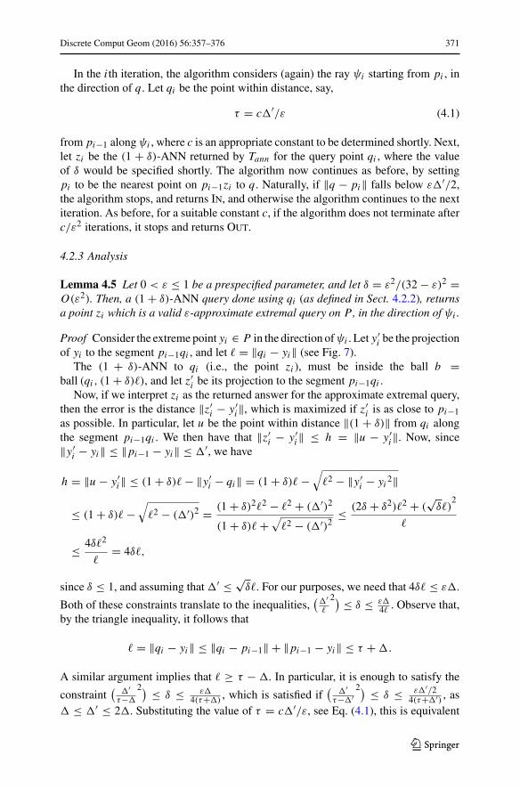
Lemma 4.5 Let 0 < ε ≤ 1 be a prespecified parameter, and let δ = ε2/(32 − ε)2 =O(ε2). Then, a (1 + δ)-ANN query done using qi (as defined in Sect. 4.2.2), returnsa point zi which is a valid ε-approximate extremal query on P, in the direction of ψi .

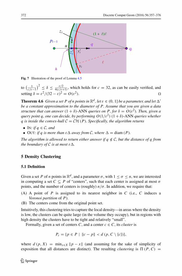
Proof Consider the extreme point yi ∈ P in the direction ofψi . Let y′i be the projection

of yi to the segment pi−1qi , and let � = ‖qi − yi‖ (see Fig. 7).The (1 + δ)-ANN to qi (i.e., the point zi ), must be inside the ball b =

ball (qi , (1 + δ)�), and let z′i be its projection to the segment pi−1qi .Now, if we interpret zi as the returned answer for the approximate extremal query,

then the error is the distance ‖z′i − y′i‖, which is maximized if z′i is as close to pi−1

as possible. In particular, let u be the point within distance ‖(1 + δ)‖ from qi alongthe segment pi−1qi . We then have that ‖z′i − y′

i‖ ≤ h = ‖u − y′i‖. Now, since‖y′

i − yi‖ ≤ ‖pi−1 − yi‖ ≤ ′, we have

h = ‖u − y′i‖ ≤ (1 + δ)� − ‖y′

i − qi‖ = (1 + δ)� −√

�2 − ‖y′i − yi 2‖

≤ (1 + δ)� −√

�2 − (′)2 = (1 + δ)2�2 − �2 + (′)2

(1 + δ)� +√

�2 − (′)2≤ (2δ + δ2)�2 + (

√δ�)

2

�

≤ 4δ�2

�= 4δ�,

since δ ≤ 1, and assuming that ′ ≤ √δ�. For our purposes, we need that 4δ� ≤ ε.

Both of these constraints translate to the inequalities,(

′�

2) ≤ δ ≤ ε4� . Observe that,

by the triangle inequality, it follows that

� = ‖qi − yi‖ ≤ ‖qi − pi−1‖ + ‖pi−1 − yi‖ ≤ τ + .

A similar argument implies that � ≥ τ − . In particular, it is enough to satisfy the

constraint(

′τ−

2) ≤ δ ≤ ε4(τ+)

, which is satisfied if(

′τ−′

2) ≤ δ ≤ ε′/24(τ+′) , as

≤ ′ ≤ 2. Substituting the value of τ = c′/ε, see Eq. (4.1), this is equivalent

123


pi 1q

yi

(1 + )

yiqi

h

zi

zi

u

Fig. 7 Illustration of the proof of Lemma 4.5

to( 1c/ε−1

)2 ≤ δ ≤ ε/24(c/ε+1) , which holds for c = 32, as can be easily verified, and

setting δ = ε2/(32 − ε)2 = O(ε2). ��Theorem 4.6 Given a set P of n points inRd , let ε ∈ (0, 1] be a parameter, and let′be a constant approximation to the diameter of P. Assume that you are given a datastructure that can answer (1 + δ)-ANN queries on P, for δ = O(ε2). Then, given aquery point q, one can decide, by performing O(1/ε2) (1+ δ)-ANN queries whetherq is inside the convex-hull C = CH (P). Specifically, the algorithm returns

• In: if q ∈ C, and• Out: if q is more than ε away from C, where = diam (P).

The algorithm is allowed to return either answer if q /∈ C, but the distance of q fromthe boundary of C is at most ε.

5 Density Clustering

5.1 Definition

Given a set P of n points inRd , and a parameter σ , with 1 ≤ σ ≤ n, we are interestedin computing a set C ⊆ P of “centers”, such that each center is assigned at most σ

points, and the number of centers is (roughly) n/σ . In addition, we require that:

(A) A point of P is assigned to its nearest neighbor in C (i.e., C induces aVoronoi partition of P).

(B) The centers come from the original point set.

Intuitively, this clustering tries to capture the local density—in areas where the densityis low, the clusters can be quite large (in the volume they occupy), but in regions withhigh density the clusters have to be tight and relatively “small”.

Formally, given a set of centers C , and a center c ∈ C , its cluster is

Pc = {p ∈ P | ‖c − p‖ < d (p,C \ {c})},

where d (p, X) = minx∈X ‖p − x‖ (and assuming for the sake of simplicity ofexposition that all distances are distinct). The resulting clustering is �(P,C) =

123


{Pc | c ∈ C }. A set of points P , and a set of centers C ⊆ P is a σ -density clusteringof P if for any c ∈ C , we have |Pc| ≤ σ . As mentioned, we want to compute abalanced partitioning, i.e., one where the number of centers is roughly n/σ . We showbelow that this is not always possible in high enough dimensions.

5.1.1 A Counterexample in High Dimension

Lemma 5.1 For any integer n > 0, there exists a set P of n points in Rn, such that

for any σ < n, a σ -density clustering of P must use at least n − σ + 1 centers.

Proof Let n be a parameter. For i = 1, . . . , n, let �i = √1 − 2−i−1, and let pi be

a point of Rn that has zero in all coordinates except the i th one, where its value

is �i . Let P = {p1, . . . , pn} ⊆ Rn . Now, di, j = ∥

∥pi − p j∥

∥ =√

�2i + �2j =√2 − 2−i−1 − 2− j−1. For i < j and i ′ < j ′, we have

di, j < di ′, j ′ ⇐⇒ 2 − 2−i−1 − 2− j−1 < 2 − 2−i ′−1 − 2− j ′−1

⇐⇒ 2−i ′ + 2− j ′ < 2−i + 2− j

⇐⇒{

i = i ′ and j < j ′, ori < i ′.

That is, the distance of the i th point to all the following points Si+1 = {pi+1, . . . , pn}is smaller than the distance between any pair of points of Si+1.

Now, consider any set of centersC ⊆ P , and let c = pi be the point with the lowestindex that belongs to C . Clearly, Pc = (P \ C) ∪ {c}; that is, all the non-center pointsof P , get assigned by the clustering to c, implying the claim. ��

5.2 Algorithms

5.2.1 Density Clustering via Nets

Lemma 5.2 For any set of n points P in Rd , and a parameter σ < n, there exists a

σ -density clustering with Od( n

σlog n

σ

)

centers.

Proof Consider the hypercube [−1, 1]d . Cover its outer faces (which are (d − 1)-dimensional hypercubes) by a grid of side length 1/3

√d. Consider a cell C

in this grid—it has diameter ≤ 1/3, and it is easy to verify that the coneφ = {tp | p ∈ C, t ≥ 0} formed by the origin and C has angular diameter < π/3.This results in a set C of N = O(dd) cones covering R

d .Fix a cone φ ∈ C. For a point p ∈ R

d , let φp denote the translation of φ such that pis its apex. Note that φ is formed by the intersection of 2(d − 1) halfspaces. As such,the range space consisting of all ranges φp, such that p ∈ R

d , has VC dimension at mostd ′ = O(d2 log d) [12, Theorem 5.22]. For a radius r and point p, let aφ-slice be the setsφ(p, r) = φp ∩ ball (p, r), i.e. the set formed by intersecting φp with a ball centeredat p and of radius r . The range space of all φ-slices, Sφ = {sφ(p, r)|p ∈ R

d , r ≥ 0},

123


Fig. 8 φ-slices are pseudo-disks

has VC dimension d ′′ = O(d +2+d ′) = O(d2 log d), since the VC dimension of ballsin R

d is d + 2, and one can combine range spaces as done above, see the book [12]for background on this.

Now, for ε = (σ/N )/n = σ/(nN ), consider an ε-net R of the point set P for

φ-slices. The size of such a net is |R| = O(

(d ′′/ε) log ε−1) = O

( nNd2 log dσ

log nNσ

) =O

(

dO(d) nσlog n

σ

) = Od( n

σlog n

σ

)

, by the ε-net theorem.Consider a point p ∈ P that is in R. Let νφ be the nearest point to p in the set

{R \ {p}} ∩ φp. The key observation is that any point in P ∩ φp that is farther awayfrom p than νφ , is closer to νφ than to p; that is, only points closer to p than νφ

might be assigned to p in the Voronoi clustering. Since R is an ε-net for φ-slices,sφ(p, ‖p − νφ‖) = φp ∩ ball (p, ‖p − νφ‖), contains at most εn = σ/N points ofP . It follows that at most σ/N points of P ∩ φp are assigned to the cluster associatedwith p. By summing over all N cones, at most (σ/N )N = σ points are assigned top, as desired. ��

5.2.2 The Planar Case

Lemma 5.3 For any set of n points P in R2, and a parameter σ with 1 ≤ σ ≤ n,

there exists a σ -density clustering with O (n/σ) centers.

Proof Consider the plane, and fix a cone φ ∈ C as used in the proof of Lemma 5.2.For a point p ∈ R

2, and a radius r , let φp denote the translated cone having p as anapex, and let sφ(p, r) = φp ∩ ball (p, r) be a φ-slice induced by this cone. Considerthe set of all possible φ-slices in the plane:

Sφ = {sφ(p, r) | p ∈ R2, r ≥ 0}.

It is easy to verify that the family Sφ behaves like a system of pseudo-disks; that is,the boundary of a pair of such regions intersects in at most two points (see Fig. 8). Assuch, the range space having P as the ground set, and Sφ as the set of possible ranges,has an ε-net of size O(1/ε) [19]. Let ε = (σ/N )/n, as in the proof of Lemma 5.2,where N = |C|. Computing such an ε-net, for every cone of C, and taking their unionresults in the desired set of cluster centers. ��Acknowledgments N.K. would like to thank Anil Gannepalli for telling him about Atomic ForceMicroscopy. The full paper is available online [14]. Work on this paper by S. Har-Peled was partially

123


supported by NSF AF Awards CCF-1421231, and CCF-1217462. Work on this paper by N. Kumar waspartially supported by a NSF AF Award CCF-1217462 while the author was a student at UIUC, and by NSFGrant CCF-1161495 and a grant from DARPA while the author has been a postdoc at UCSB. Work on thispaper by D. M. Mount was partially supported by NSF Award CCF-1117259 and ONR Award N00014-08-1-1015. Work on this paper by B. Raichel was partially supported by NSF AF Awards CCF-1421231,CCF-1217462, and the University of Illinois Graduate College Dissertation Completion Fellowship.

References

1. Andersson, L.-E., Stewart, N.F.: Introduction to the Mathematics of Subdivision Surfaces. SIAM,Philadelphia (2010)

2. Barman, S.: Approximating nash equilibria and dense bipartite subgraphs via an approximate versionof Caratheodory’s theorem. In: Proceedings of 47th Annual Symposium on the Theory of Computing(STOC), pp. 361–369 (2015)

3. Basu, S., Pollack, R., Roy,M.F.: Algorithms in Real Algebraic Geometry. Algorithms andComputationin Mathematics. Springer, Berlin (2006)

4. Binnig, G., Quate, C.F., Gerber, Ch.: Atomic force microscope. Phys. Rev. Lett. 56, 930–933 (1986)5. Blinn, J.F.: A generalization of algebraic surface drawing. ACM Trans. Graph. 1, 235–256 (1982)6. Boissonnat, J.-D., Guibas, L.J., Oudot, S.: Learning smooth shapes by probing. Comput. Geom. Theory

Appl. 37(1), 38–58 (2007)7. Clarkson, K.L.: Coresets, sparse greedy approximation, and the Frank–Wolfe algorithm. ACM Trans.

Algorithms 6(4), 63 (2010)8. Cole, R., Yap, C.K.: Shape from probing. J. Algorithms 8(1), 19–38 (1987)9. Feder, T., Greene, D. H.: Optimal algorithms for approximate clustering. In: Proceedings of 20th

Annual ACM Aymposium on Theory of computing (STOC), pp. 434–444 (1988)10. Goel, A., Indyk, P., Varadarajan, K. R.: Reductions among high dimensional proximity problems. In:

Proceedings of 12th ACM–SIAM Symposium on Discrete Algorithms (SODA), pp. 769–778, (2001)11. Gonzalez, T.: Clustering to minimize the maximum intercluster distance. Theor. Comput. Sci. 38,

293–306 (1985)12. Har-Peled, S.: Geometric Approximation Algorithms. Mathematical Surveys and Monographs, vol.

173. American Mathematical Society, Providence (2011)13. Har-Peled, S., Indyk, P., Motwani, R.: Approximate nearest neighbors: towards removing the curse of

dimensionality. Theory Comput. 8, 321–350 (2012). Special issue in honor of Rajeev Motwani14. Har-Peled, S., Kumar, N., Mount, D., Raichel, B.: Space exploration via proximity search. CoRR,

http://arxiv.org/abs/1412.1398 (2014)15. Har-Peled, S., Mendel, M.: Fast construction of nets in low dimensional metrics, and their applications.

SIAM J. Comput. 35(5), 1148–1184 (2006)16. Indyk, P.: Nearest neighbors in high-dimensional spaces. In: Goodman, J.E., O’Rourke, J. (eds.) Hand-

book of Discrete and Computational Geometry, Chapter 39, 2nd edn, pp. 877–892. CRC Press, BocaRaton (2004)

17. Kalantari, B.: A characterization theorem and an algorithm for a convex hull problem. Ann. Oper. Res.226(1), 301–349 (2015)

18. Mandelbrot, B.B.: The Fractal Geometry of Nature. Macmillan, New York (1983)19. Matoušek, J., Seidel, R., Welzl, E.: How to net a lot with little: small ε-nets for disks and halfspaces. In:

Proceedings of 6th Annual ACM Symposium on Computational Geometry (SoCG), pp. 16–22 (1990)20. Mulvey, J.M., Beck, M.P.: Solving capacitated clustering problems. Eur. J. Oper. Res. 18, 339–348

(1984)21. Novikoff, A.B.J.: On convergence proofs on perceptrons. Proc. Symp. Math. Theo. Automata 12,

615–622 (1962)22. Panahi, F., Adler, A., van der Stappen, A. F., Goldberg, K.: An efficient proximity probing algorithm for

metrology. In: Proceedings of IEEE International Conference on Automation Science and Engineering(CASE), pp. 342–349 (2013)

23. Smelik, R. M., De Kraker, K. J., Groenewegen, S. A., Tutenel, T., Bidarra, R.: A survey of proceduralmethods for terrain modelling. In: Proceedings of the CASA. Workshop on 3D Advanced Media InGaming and Simulation (2009)

24. Skiena, S.S.: Problems in geometric probing. Algorithmica 4, 599–605 (1989)

123

http://arxiv.org/abs/1412.1398


25. Skiena, S.S.: Geometric reconstruction problems. In: Goodman, J.E., O’Rourke, J. (eds.) Handbook ofDiscrete and Computational Geometry, Chapter 26, pp. 481–490. CRC Press LLC, Boca Raton (1997)

26. Wikipedia. Atomic force microscopy—Wikipedia, The Free Encyclopedia (2014)

123

space exploration via proximity search - umd

Documents