Spare Parts Requirements for Space Missionswith Reconfigurability and Commonality

Afreen Siddiqi∗ and Olivier L. de Weck†

Massachusetts Institute of Technology, Cambridge, Massachusetts 02139

DOI: 10.2514/1.21847

The logistics resources (in the form of spare parts) for future explorationmissions to the moon andMars can have

significant mass and volume requirements. In this study it is shown that reconfigurable or common parts that allow

use of the same component indifferentmission elements, canbe ameans of reducing the requirednumber of spares. A

model for determining the system availability as a function of spares level is developed for a mission that utilizes

elements with reconfigurable or common parts. An explicit consideration of the operating scenario is made that

allows the use of components from elements that are not operating at a given time. A Mars surface exploration

mission is used to illustrate the application of this model. It is shown, for the specific example studied in the analysis,

that the same level of system availability can be achievedwith 33–50% fewer spares if the parts are reconfigurable or

common across different mission elements.

Nomenclature

A�ti� = availability at ti�B�ti� = expected backorder level at ti�Bc�s; ti� = expected backorder level at ti for spares level sE = number of total elements in the missionl = failure rate (failures per day)N = total number of units among all elements and

including spares repositoryP�s� = probability of having s spares availablep�n� = probability of n failuresqe = no. of units of a component in element es = total number of sparessE = maximum number of spares available from idle

elementssI = initial number of spares in repositoryti = time instances at which operating elements change

their state�e�tk� = binary variable with value 1 if element e is

operating in interval tk��ti� = percentage of elements operating at ti� = mean number of failures

I. Introduction

F UTURE humanmissions to themoon andMars can be expectedto use several elements. Typical elements comprising a surface

mission may include ascent/descent vehicles, rovers for surfacemobility, and habitats for long duration surface stays (see Fig. 1).

In such largemissions, the required logistics resources can becomesignificant. Common or reconfigurable spare parts, which can beconfigured to function in different systems as required, canpotentially be of great benefit. The mass and volume of logisticsresources (spare parts) needed for an exploration mission can be

greatly reduced through the use of such components. Furthermore,other maintenance and operation procedures can become easier dueto commonality of components in different elements.

This paper develops a model for estimating the requirements ofreconfigurable spare parts needed for systems that may not beoperating concurrently. It then explores the amount of benefit thatcan be achieved in logistical costs through this reconfigurability. Akey consideration made in the model is that of the operationalscenario of the various elements. It is assumed that all elementsinvolved in the mission do not necessarily operate simultaneously,for example, the ascent/descent vehicle and all the rovers do not haveto operate at the same instance of time in the mission. A greater reuseof components therefore becomes possible. It should be noted,however, that the elements between which the parts are exchangedhave to be in close proximity. In such a case, a functional part from anonoperating (or idle) element can thus be borrowed or scavengedfor installation on an operating element that has experienced a

failure.

It is also assumed that there is a set of spare parts that are brought inwith themission and are utilizedfirst as failures occur. The parts fromidle elements are only reused on other operating elements if no newspares are available. The interchange of parts does not take placeroutinely, rather it is done as a last resort.

It should be noted that the case of commonality, that is, commonparts among different elements is implicitly included in this work.The difference between the reconfigurable case and the common caseis simply that in the former the parts will need to undergo areconfiguration in some fashion before being installed on anotherelement, while in the latter (i.e., in the commonality case) the partscan simply be used as is. So the samemodel applies to both cases, andthe difference canmanifest itself in the form of altered failure rates ofthe components or repair and service times. In general, it can beexpected that in the reconfigurable case the failure rates and servicetimes will be comparatively higher than the commonality case,however, this may not always be true.

Literature review: Several models have been produced foranalyzing spare parts inventory requirements. Caglar and Simchi-Levi [1] have shown how a two-echelon spares parts inventorysystem can bemodeled and optimally solved for a given service timeconstraint. Shishko [2] has modeled costs of spares and repairs inestimating operations costs for the International Space Station.Bachman and Kline [3] have developed a model for estimating spareparts requirements for space exploration missions.

The model presented in [3] is used in this work as a base case(which is referred to as the “dedicated case” in this study) in whichcomponents are assumed to be used for only particular elements. Anenhancedmodel is then formulated inwhich the parts can be assumed

Received 16 December 2005; revision received 9 March 2006; acceptedfor publication 9 March 2006. Copyright © 2006 by Olivier de Weck andAfreen Siddiqi. Published by the American Institute of Aeronautics andAstronautics, Inc., with permission. Copies of this paper may be made forpersonal or internal use, on condition that the copier pay the $10.00 per-copyfee to the Copyright Clearance Center, Inc., 222 Rosewood Drive, Danvers,MA 01923; include the code $10.00 in correspondence with the CCC.

∗Graduate Student, Department of Aeronautics & Astronautics, Room 33-409, AIAA Student Member.

†Assistant Professor of Aeronautics & Astronautics and EngineeringSystems, Department of Aeronautics & Astronautics, Engineering SystemsDivision, Room33-410, 77Massachusetts Avenue, deweck@mit.edu, AIAASenior Member.

JOURNAL OF SPACECRAFT AND ROCKETS

Vol. 44, No. 1, January–February 2007

147

to be reconfigurable (or common) and thus an interchange of partsbetween mission elements subject to their operational state ispermitted. The overall system availability is then formulated and anexplicit provision of using components from idle elements isincluded. A sensitivity analysis is also performed for some limitedcases to assess the impact of various parameters (such as componentreliability and the operational scenario) on system availability.

II. Model for Estimating Requirements ofReconfigurable Spare Parts

A total of E, colocated elements are considered to be part of themission. Although each element is composed of several subsystemsand parts, for simplicity only one type of part is considered first here(the extension for several parts is discussed at the end of the section).It is assumed that there is no resupply (which is conceivable for amission to Mars for instance), so no additional parts can be madeavailable during the course of the mission. Furthermore, no repaircapability is assumed. Thus, once a part fails it cannot be employedfor use at a later time.

Figure 2 illustrates the usage model assumed for dedicated andreconfigurable parts. It shows that if elements are using dedicatedcomponents, then only particular spares designed for a particularelement can be used from a spares repository. On the other hand,operating elements in need of reconfigurable (or common) spares canobtain the parts from either a spares repository or an idle element (asindicated with the dashed oval).

In the following sections a model for estimating spare partsrequirements for elements using dedicated components is firstdiscussed, and then a model in which reconfigurable/common spareparts are used is developed in an analogous fashion.

A. Dedicated Spare Parts

In this case the component used in each element will be for thededicated use of only that element. For simplicity, consider that thereis only one type of component installed on element j (Fig. 2a). Thequantity per application (QPA), which is the number of units of thecomponent used, will be denoted as qj. It is assumed that there is aspare parts repository which is a collection of spares for the variousmission elements. The spares level for each element’s component inthat repository is sj. The sumof all sj is sI which is the total number ofspares initially in the repository at the start of the mission.

It is considered that the components fail according to a Poissonprocess described by

pj�n� �e��j�n

j

n!(1)

�j �Z

tf

to

ljdt (2)

where pj�n� is the probability of having exactly n failures of thecomponent in element j in interval �totf � for a process that has afailure rate of lj, which is the inverse of its mean time to failure(MTTF). The mean of such a Poisson process can be shown to beequal to�j. If there areqj units, and lj is independent of time, then themean number of failures in interval �totf� is simply

�j � qjlj�tf � to� (3)

and is sometimes referred to as “outstanding orders” [1], or as the“number in the pipeline” [3]. Note that the interval �totf � is theduration the component has operated for. The expected backorder

level, �Bj, is the expected value of the difference between the actualnumber of spares that are available and the required number of spares(as driven by the number of failed components). It is thereforecomputed as [3]

�B j �X1n>sj

�n � sj�pj�n� (4)

In reality the upper bound on the summation is the total failures thatcan occur of the component.

In this case redundancy in an element is ignored, and it is assumedthat an element is operational if it does not have any outstanding

requests for replacing any failed component, that is, its �B is zero. If it

Fig. 1 Typical space exploration mission elements.

a) Dedicated spares for particular elements

b) Reconfigurable spares for any element

Fig. 2 Dedicated and reconfigurable spares usability by elements.

148 SIDDIQI AND DE WECK

is assumed that the backorders of the part are uniformly distributedacross the elements, then the probability that there is an outstanding

request for a component in a particular element is �Bj=qj. The failuresof the components in the different elements are considered to beindependent, and thus the availability (of the element that uses thiscomponent) is

Aj ��1�

�Bj

qj

�qj

(5)

It should be noted thatA is the availability that can be expected at theend of time tf since it was used for evaluating � given in Eq. (3). Thesystem availability can be defined as the probability of all of theelements that should be operating to be actually operational. Theoverall availability is then simply the product of availability of all theelements (assuming that all the elements need to be fully operationalfor the entire mission)

Asys �YEj�1

Aj (6)

Ifmore than one component needs to be considered in the analysis,this model is easily extended by using Eq. (5) for each componentand then taking the product to get element availability (assuming thatall of those components have to be operational for the element to beconsidered available). However, this can get more complex ifredundancy is also modeled.

B. Reconfigurable Spare Parts

The above approach is the traditional analysis in which it wasassumed that elements use dedicated components and hence havecorresponding dedicated spares for maintenance. A spares inventorystock level for a repository can be estimated by analyzing failure ratesand operation duration and other desired constraints (such as meandelivery times, etc.) for a mission.

Now consider the case where it is assumed that reconfigurablecomponents are used, and a particular component can be eitherreconfigured (or utilized as is) for use on a variety of differentelements in the mission (Fig. 2b). A specific instance of thecomponent installed on one element that is not operating for a periodof time during the mission can therefore be employed on a differentelement that may need it (which is also referred to as temporaryscavenging or cannibalization) when all the spares from theinventory have been depleted. In such a scenario, an element e,during its idle time, that is, the time when it is not operating, can thenbe viewed as a potential spares repository that can supply amaximumof qe spares if required (where qe is the QPA of that component inelement e). In such a situation (and assuming the elements arecolocated) there is not just one warehouse of spares, but also othertemporal repositories that can supply limited quantities of spares atcertain points over the course of the mission. It needs to beemphasized that the existence of those repositories is a function of themission time. Furthermore, the spares from these temporalrepositories are not necessarily new, rather they may have operatedfor a period of time.

The system availability will be based on the number of potentialspares that can be obtained from the initial spares repository as wellas idle mission elements and will thus be affected by the operationalscenario. The operating time profile of each element over the courseof the mission therefore has to be first considered. Using thisinformation, a set of time instances can then be defined:

T � �t1; . . . ; ti; . . . ; tn� (7)

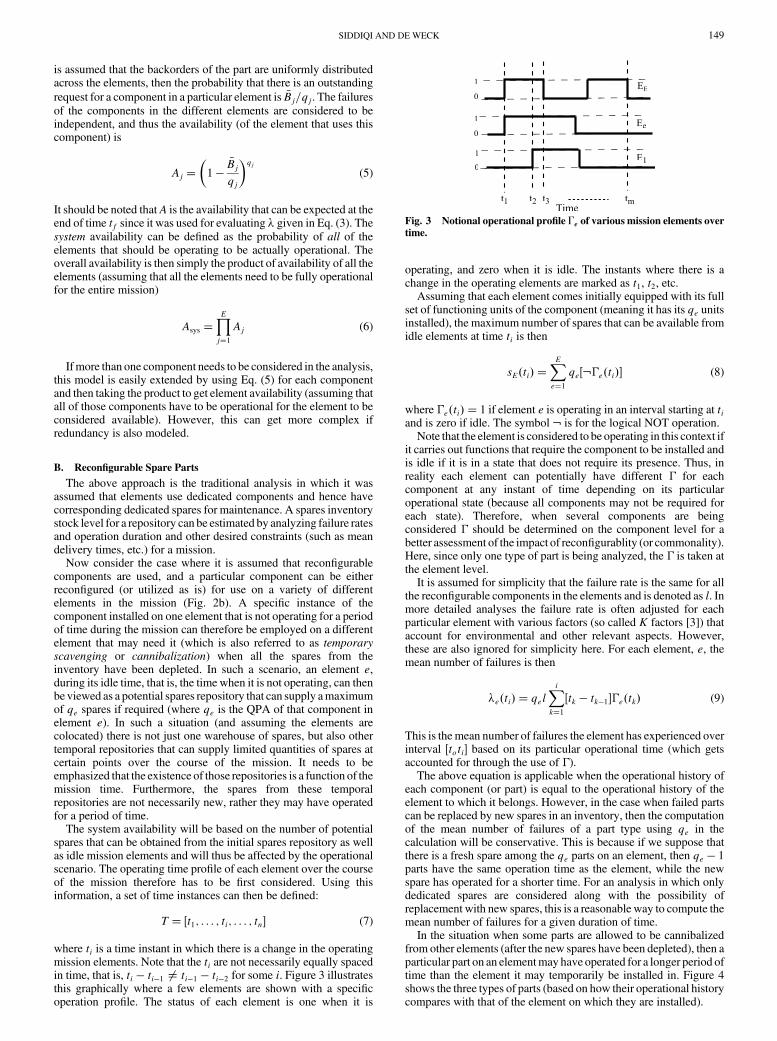
where ti is a time instant in which there is a change in the operatingmission elements. Note that the ti are not necessarily equally spacedin time, that is, ti � ti�1 ≠ ti�1 � ti�2 for some i. Figure 3 illustratesthis graphically where a few elements are shown with a specificoperation profile. The status of each element is one when it is

operating, and zero when it is idle. The instants where there is achange in the operating elements are marked as t1, t2, etc.

Assuming that each element comes initially equipped with its fullset of functioning units of the component (meaning it has its qe unitsinstalled), the maximum number of spares that can be available fromidle elements at time ti is then

sE�ti� �XEe�1

qe�:�e�ti�� (8)

where �e�ti� � 1 if element e is operating in an interval starting at tiand is zero if idle. The symbol : is for the logical NOT operation.

Note that the element is considered to be operating in this context ifit carries out functions that require the component to be installed andis idle if it is in a state that does not require its presence. Thus, inreality each element can potentially have different � for eachcomponent at any instant of time depending on its particularoperational state (because all components may not be required foreach state). Therefore, when several components are beingconsidered � should be determined on the component level for abetter assessment of the impact of reconfigurablity (or commonality).Here, since only one type of part is being analyzed, the � is taken atthe element level.

It is assumed for simplicity that the failure rate is the same for allthe reconfigurable components in the elements and is denoted as l. Inmore detailed analyses the failure rate is often adjusted for eachparticular element with various factors (so called K factors [3]) thataccount for environmental and other relevant aspects. However,these are also ignored for simplicity here. For each element, e, themean number of failures is then

�e�ti� � qelXi

k�1

�tk � tk�1��e�tk� (9)

This is the mean number of failures the element has experienced overinterval �toti� based on its particular operational time (which getsaccounted for through the use of �).

The above equation is applicable when the operational history ofeach component (or part) is equal to the operational history of theelement to which it belongs. However, in the case when failed partscan be replaced by new spares in an inventory, then the computationof the mean number of failures of a part type using qe in thecalculation will be conservative. This is because if we suppose thatthere is a fresh spare among the qe parts on an element, then qe � 1parts have the same operation time as the element, while the newspare has operated for a shorter time. For an analysis in which onlydedicated spares are considered along with the possibility ofreplacement with new spares, this is a reasonable way to compute themean number of failures for a given duration of time.

In the situation when some parts are allowed to be cannibalizedfrom other elements (after the new spares have been depleted), then aparticular part on an elementmay have operated for a longer period oftime than the element it may temporarily be installed in. Figure 4shows the three types of parts (based on how their operational historycompares with that of the element on which they are installed).

Fig. 3 Notional operational profile �e of various mission elements overtime.

SIDDIQI AND DE WECK 149

In this case, Eq. (9) is appropriate if the cannibalization wouldoccur very rarely. In that situation, the possibility of having a part onan element that has operated longer than the element it is installed onwill be very low, and Eq. (9) can still be applicable with some degreeof caution. However, if the cannibalization can happen frequently(perhaps due to a combination of high failure rates and fewer newspares, etc.), then the problem can be analyzed in two ways. It caneither be simulated (in which the operational and element installationhistory of each part will be known explicitly), or a more conservativeestimate of the mean failures is made by noting that the operationtime of any part at a time instance cannot exceed the total missiontime elapsed up to that time. In that case

�e�ti� � qelXi

k�1

�tk � tk�1� (10)

Note that this bound can give significantly conservative results if theoperation duration of an element is much less than the total missiontime. However, this simplification allows an analytical assessment(instead of simulation) when the chances of cannibalization are greatenough that the subsequent effect on the part failure rate cannot beignored.

The mean number of failed components of a particular type fromall the elements in interval �toti� is

��ti� �XEe�1

�e�ti� (11)

If the total number of failures (which is a random variable) up to agiven time instance is nF, then the number of total spares (which isalso a random variable) is

s�ti� � sI � sE�ti� � nF (12)

The term sI denotes the initial quantity of spares in an actualrepository, whereas sE�ti� as described earlier is the additional sparesthat can be provided by the various idle elements (which act aspseudorepositories). If nF > sI � sE�ti�, then s�ti� is zero.

The number of failures nF can assume integer values ranging from0 to N, where N is the total units of the component in the mission

N � sI �Q (13)

Q�XEe�1

qe (14)

The random variable s�ti� can also take integer values that areaccording to Eq. (12). For zero failures it can have a maximum valueof sI � sE�ti�, or it can have aminimum value of zero if no spares areavailable.

In the dedicated case each element has its own set of spares, andtherefore the spares level sj for each element j is used to determine itsparticular backorder level. In the augmented model withreconfigurable or common parts, because all the elements aresupplied with replacement parts from a total of s�ti� spares, thebackorder levels are computed at the mission level (across all

elements). The expected backorder level at ti, for the condition whenthe total spares level is s, is then

�B c�s; ti� �XN

nF�s�1

�nF � s�p�nF� (15)

The expected backorder level after accounting for all the possiblevalues of s is then

�B�ti� �XSs�0

�Bc�s; ti�P�s� (16)

�B�ti� �XSs�0

�P�s�

XNnF�s�1

�nF � s�p�nF��

(17)

where S is the maximum value of the total spares level at time ti(corresponding to zero failures). The probability P�s� is equal to theprobability ofnF failures occurringwhich result in a spares level s [asgiven by Eq. (12)]. For instance, if the possible values of s�ti� in aninterval are 0, 1, and 2, then the conditional backorder levels �Bc�0�,�Bc�1�, and �Bc�2� which correspond to each possible value of s arecomputed. The values are then multiplied with P�0�, P�1�, and P�2�and summed to get the overall backorder level �B�ti�.

The probability of a total of nF failures taking place up to a time tiin the mission across all the elements is computed by considering allthe possible ways in which that number of failures can occur, forinstance, if there are twomission elements andnF is 2. There are threepossible ways in which a total of two failures can occur. In the firstcase there can be two failures in the first element and none in thesecond, or in a second case there can be no failures in the first elementand two in the second, or in the third case there can be one failure eachin the two elements. In all these scenarios the total number of failuresis the same; however, each individual element has a different numberof failures. The number of failures that an element e experiences in aparticular scenario w will be denoted as nw

e . The probability of anyindividual scenariow occurring is the product of the probabilities ofthe specific failures occurring in each element in that particularscenario (assuming the failures are independent).

Pw �YEe�1

p�nwe � (18)

For instance, in the example described above, the probability of thefirst scenario taking place is the product of the probability of havingtwo failures in the first element and the probability of having nofailures in the second element. The probability of having nw

e failuresin element e is the Poisson probability

p�nwe � �

e��e�nwe

nwe !

(19)

The argument ti has been omitted from �e for simplicity here. Theprobability of having nF failures occur across all the missionelements is then the sum of probabilities of all the various ways inwhich it can happen. Therefore

p�nF� �XWw�1

Pw (20)

whereW is the number of all the combinations in which a total of nF

failures can occur from among E elements with a total of Qcomponents. It should be noted that P�s� can be computed in asimilar fashion as p�nF�.

Using Eq. (17), the overall availability at ti is then simply

Asys�ti� ��1 �

�B�ti�Q

�Q

(21)

It can be observed that now the end-of-mission availability is not

Fig. 4 Types of parts that can exist in an element.

150 SIDDIQI AND DE WECK

directly relevant (which is usually the case in traditional studies).A isno longer a monotonically decreasing function of time due to theexplicit consideration of making use of components from otherelements. The end-of-mission availability may be higher due tomorespares being potentially available if fewer elements are operating,while the availability at some intermediatemission timemaybe lowerwhen more elements are operating at that time. The availability foreach interval can be computed using the above equation. Because theworst case scenario is often of interest, the mission level availabilityfor this reconfigurable spare parts case can then be taken as theminimum system availability that occurs at any time during themission duration.

Asys �min�Asys�ti�� ti 2 T (22)

III. Monte Carlo Simulation

The validity of this model for reconfigurable or common sparescan be tested through a discrete-event simulator. Furthermore, asdiscussed previously, a simulator can serve to assess theconservativeness of the assumptions regarding part operation timesfor Eq. (10).

In the simulation, the failure of parts installed on a set of givenmission elements (Fig. 1) is simulated as a Poisson process (with thedetails as discussed in the previous section). Each part is allowed tobe in one of three different states. It can either be operating (if it is onan operating element), it can be idle (if it is either installed on an idleelement, or is in the spares repository), or it can be in a failed state.Once the part has failed, it cannot be repaired.

If a part fails, it is replaced immediately with a spare part from therepository if one is available. These spares are new and thereforehave not operated for any duration of time until they are installed onan element. Their probability of failure at any day will therefore bedifferent (and lower) than the failure probability of other parts thathave been working in the element for longer periods of time. Note,that as failures occur during the mission, the fresh spares from therepository are first used. If there are more failures and the sparesrepository is empty, only then parts from idle elements are takenaway to be installed on operating elements that need them. Thecannibalization of idle elements is thus done as a last resort when allthe new spares have been used up. In the simulation thecannibalization is done randomly from the first idle part that is found.In a more realistic case, priorities can be assigned to elements so thatrelatively less critical elements can bemore readily cannibalized thanthe more critical ones (because cannibalization can lead to newproblems and potential failures of other parts in the element).

If at any time instance, there are more spares required than areavailable, then the spares are allocated to the elements in an optimalway such that the mission level availability is maximized. Anotheralgorithm for assigning the spares can be based on the priority levelof the mission elements. The elements with higher priority (e.g.,those that are critical for crew survivability, etc.) can be assignedspares before low priority elements are given the leftover parts.

For each simulation, a uniformly distributed random number isgenerated which is then used to determine if a part fails or not at eachtime step (e.g., each day of a mission). A part is allowed to fail if itsprobability of failure is greater than the random number, otherwise itis allowed to continue operation and its operational time isincremented by one time step.

If there is a failure, the part is replaced with either new or usedspares according to the procedure described above. If there are noparts that can be installed in place of the failed one, the element onwhich the part failed is considered to be unavailable or down.

Even if a failure does not occur in a particular time step, but anelement is down (when it should be operational), the availability ofspares is checked and appropriate assignments are made if possible.Because the spare parts are a function of time due to the operationalscenario of the elements, an element may be down due to lack ofspare parts for some duration of the mission, but it may be able to

function again later on if some other element becomes idle and itsparts become available for temporary cannibalization.

Each simulation run of a specific mission (over a certain missiontime line) plays out one particular outcome that can unfold.Hundredsof such simulations therefore need to be carried out so that a statisticalanalysis can be done to assess how the availability of the elementscompares with the analytical predictions. Section V will discuss theresults of a case study, in which the model predictions and simulatedresults will be compared for a sample exploration mission.

IV. Sensitivity Analysis

It can be seen that the system availability [Eq. (22)] is a function offailure rate l, QPA, operational scenario �, and spares level, sI . For agiven value of sI (which are the number of spares brought initially atthe start of themission), it can be useful to assess how the availabilityvaries with the other parameters.

A. Availability and Quantity

For finite values of q, Eq. (5) can be used for determining how Achangeswith q. However, using the general relation (for a variable x)

limn!1

�1� x

n

�n

� ex (23)

it can be seen that if q becomes large (i.e., many units of the samecomponent are used) then the availability is simply an exponentialfunction of the backorder level.

limq!1

A� limq!1

�1�� �B

q

�q

(24)

� e� �B (25)

Thus, availability can decrease extremely rapidly if the backorderlevel makes even a modest climb.

B. Availability and Failure Rate

1. Dedicated Case

For the case of dedicated components, the availability of anelement is given by Eq. (5) which is reproduced below.

A��1 �

�B

q

�q

The subscripts i and e have been dropped becausewe are consideringonly one element and one component in that element. The derivativeof A with respect to the failure rate l can be expressed as

dA

dl� q

�1�

�B

q

�q�1�

� 1

q

d �B

dl

�(26)

� qA

�q � �B�=q

�� 1

q

d �B

dl

�(27)

� Aq

� �B � q�d �B

dl(28)

� Aq

� �B � q�

�d

dl

�Xn>s

�n � s�p�n���

(29)

Since l is the variable of interest, a constant � in this context can bedefined

�� q�t (30)

where�t is the total duration of time for which the element operated.The number in the pipeline is then

SIDDIQI AND DE WECK 151

�� �l (31)

Equation (29) can then be written as

dA

dl� Aq

� �B � q�

�Xn>s

�n � s�n!

d

dlfe��l��l�ng

�(32)

dA

dl� Aq

� �B � q�

�Xn>s

�n � s�p�n��n

l� �

��(33)

As expected, the rate of change ofAwith respect to l is negative since�B cannot be greater than q. Thus the availability decreases withincreasing failure rate.

2. Reconfigurable Case

In the reconfigurable case, a similar procedure for determining thederivative from the availability equation can be followed. In this caseit should be recalled that the number of failures and spares availablewas computed for all the elements combined at the mission level.Therefore to be able to compare the dA=dl at the element levelbetween the two cases, it is assumed for the reconfigurable case thatthe variable s denotes the spares level that a particular element canuse. Because the objective of this analysis is to simply compare thesensitivity expressions of availability with the failure rate, thisassumption is reasonable in this context. If subscript r is used for thereconfigurable case, then the following expression can be written forthe availability of a particular element at time ti:

dAr

dl� Arq

�Br � q

d �Br

dl(34)

Using Eq. (17), the above expression can be written as

dAr

dl� Arq

�Br � q

�XSs�0

�P�s�

Xn>s

�n � s� ddlp�n� � �Bc�s�

d

dlP�s�

��

(35)

Using the development of Eq. (32) for the derivative of p�n�, theabove equation becomes

dAr

dl� Arq

�Br � q

��XS

s�0

�P�s�

Xn>s

�n � s�p�n��n

l� �

�� �Bc�s�

d

dlP�s�

��

(36)

From the above equation and Eq. (33) it is sufficient to see that therate of change of Awith respect to l is different for the dedicated andreconfigurable cases. This difference in the sensitivities of A to l [asevident from Eqs. (33) and (36)] can become important in studyingthe tradeoffs between reconfigurable components and dedicatedcomponents versus different reliabilities. Section V provides anexample of such a case.

C. Availability and Operation Time

The model developed for the reconfigurable case makes thebackorder levels and thus availability dependent on the number ofidle elements at a given instance of time. The operational scenariocan greatly affect mission level availability. To assess the impact ofoperational times a quantity � can be defined such that it is thefraction of operating elements out of the total mission elements at aparticular time. Thus

�i �1

E

XEe�1

�e�ti� (37)

With this definition � varies between 0 (when no element isoperating) and 1 (when all elements are operating simultaneously). If

a simplifying assumption is made that all elements in the missionhave the same QPA of the component, that is, qe � q 8 e, then themaximum number of spares that can be obtained from the elementssE at time ti [shown in Eq. (8)] is

sE�ti� � qXEe�1

:�e�ti� (38)

The summation term is simply the number of idle elements at ti, so

sE�ti� � qE�1 � �i� (39)

From Eq. (12), it follows that the spares s�ti� available at instant ti isnow also a function of � and is

s�ti; �i� � sI � qE�1� �i� � nF (40)

The first term is the initial inventory or fresh spares, the second termrepresents the pseudoinventory of spares from idle elements, and thethird term in the sum is the total cumulative number of failed partsacross all elements up to time ti in the mission. The derivative of theavailability Ar of an element with respect to � at time ti can now beexpressed [in a similar fashion as Eq. (34) and with the sameassumptions] as

dAr

d�� Arq

�Br � q

d

d��Br (41)

The above equation can be expanded further as

dAr

d�� Arq

�Br � q

�XSs�0

P�s� d

d��Bc�s� � �Bc�s�

d

d�P�s�

�(42)

Now, in the dedicated case the availability is not dependent onwhich other elements are operating at a given instant of time.Therefore there is no dependence on � and

dA

d�� 0 (43)

To show that the variation of the availability with � is different for thededicated and reconfigurable/common case, it is sufficient to see thatEqs. (42) and (43) are not the same.

V. Example: Mars Exploration Mission

A case study of a planetary exploration mission can be developedfor assessing the spare parts requirements for reconfigurable and alsodedicated components. Furthermore, to test the validity of themodel,Monte Carlo simulations are carried out using a discrete-eventsimulation of the mission.

A surface exploration mission of Mars is considered in which themission elements are an ascent/descent vehicle (ADV), a surfacehabitat (HAB), an unpressurized all-terrain vehicle (ATV), and apressurized rover (PR). It is assumed that there is no resupply orrepair and all the spares that may be required during the course of themission have to be brought in along with other cargo. In the HubbleSpace Telescope, in addition to several rate sensors (gyros), a few ofits electronic control units (ECU) also failed [4,5]. Thus, as a realisticexample an ECU is taken to be the component under considerationhere. This ECU is assumed to be reconfigurable such that it can beemployed for use in any of the mission elements described above.The QPA of this ECU for the ADV, ATV, HAB, and PR are 1, 1, 3,and 2, respectively. The MTTF of this ECU is assumed to be100,000 h of operation (which is a realistic estimate). The failure ratel is then simply the reciprocal of this MTTF. Because this is a Marsmission, a surface stay of 600 days [6] is assumed (therefore themission time starts at day 1 on the surface and ends at day 600 whenthe crew departs).

A specific operational scenario is assumed, and the operation timeprofiles for the elements shown in Fig. 5a. At each time instant, avalue of 1 indicates that the element is operating, whereas a value of

152 SIDDIQI AND DE WECK

zero is shown when the element is idle. Based on these operationprofiles, the instances of time in which a change in the operatingelements occurs are determined.

It can be observed that the time instances in Fig. 5b vary widely induration, with some intervals being very small (a few days), whileothers are very large (hundreds of days).

As discussed earlier, in the reconfigurable case the systemavailability may not necessarily be the lowest at the end of themission because the number of available spares are derived from idlecomponents in addition to a spares repository [Eq. (12)]. This can beseen in this case alsowhere Fig. 6 shows that the availability is lowestin the fifth interval. This interval happens to be the longest and alsohas the most elements concurrently operating, thus making its se thelowest (as shown in Fig. 7). Because the potential number of sparesare the lowest in this interval, the availability is also the lowest. Theavailability could have been relatively higher, however, if thisoccurred earlier in the mission because the chances of part failurewould have been lower. As discussed in Eq. (22), this minimumvalue of availability over the mission duration is considered forcomparison with dedicated cases (in which only the end-of-missionavailability is evaluated).

In addition to applying the analytical model for this particular casestudy, a discrete-event simulator was also used to compare the resultsfor the reconfigurable case. Figure 8 shows the outcome of 5000simulations for an inventory spares level sI of 0 for the reconfigurablecase. It can be seen that in some cases, all four elements were not

available, despite their ability to use scavenged parts. Overall, theavailability was found to be 78.08% for this particular spares level.

The system availability as a function of inventory spares level sIwas then determined using the analytical model [with Eqs. (6) and

a) Operation time profile

1 2 3 4 5 6 7 80

50

100

150

200

250

300

350

400

450

Tim

e In

terv

als

[day

s]

Interval #

b) Time Intervals (t i − t i − 1)Fig. 5 Operation time profiles of the mission elements.

t1 t2 t3 t4 t5 t6 t7 t80.1

0.2

0.3

0.4

0.5

0.6

0.7

0.8

0.9

1

Ava

ilabi

lity

Time interval #

Availability at Time Intervals for Varying Spares Levels

Fig. 6 Availability in various time intervals for the reconfigurable case.

1 2 3 4 5 6 7 81

2

3

4

5

6

s e (#

of m

ax s

pare

s fr

om id

le e

lem

ents

)

Transition Times [mission days]

Fig. 7 Maximum spares from idle elements in various time intervals.

0 500 1000 1500 2000 2500 3000 3500 4000 4500 50001

2

3

4

Simulation #

# of

Ava

ilabl

e E

lem

ents

ove

r E

ntire

Mis

sion

Fig. 8 Simulated results of system availability (5000 runs, sI � 0).

SIDDIQI AND DE WECK 153

(22)] and the simulator. The system availability for thereconfigurable case was computed in two ways using both theconservative assumption [Eq. (10)], and relatively nonconservativeassumption [Eq. (9)], respectively.

In the dedicated case, the assumptionwas that each element had itsown particular ECU which cannot be used in the other elements.Furthermore, for each given spare level, the optimal sparescombination (for each element) that maximized the systemavailability was used. The optimal combination was computed bysimply doing a full-factorial analysis (because the number ofelements and the spares level were small). All the possiblecombinations for a total spares level (sI) to be distributed among theE elements were determined and the corresponding level ofavailability was computed. The combination that produced thehighest overall availability at the mission level was chosen for eachparticular value of sI . So, for instance, if a total of three spares werepart of the repository (sI � 3), the optimal combination of havingspares for the ADV, ATV, HAB, and PR was determined such thatthe system availability was highest for the total spare level of 3. Inthis case it worked out to be one spare each for the ATV, HAB, andPR, while none for the ADV. Details of the optimal combinations ofthe dedicated spares are given in Table 1.

Figure 9 shows how the reconfigurable and dedicated casescompare in terms of system availability as a function of initial spareslevel. A total of four lines, corresponding to a particular case, areshown. The first line from the top is the simulated result obtained foreach spares level for the reconfigurable case. The second line fromthe top shows the analytical result from the model using thenonconservative approach for computing �e [(Eq. (9)]. As expected,it gives a lower prediction for the availability as compared to thesimulated case. However, the third line which is the analyticalprediction using the conservative value for � [Eq. (10)], is the moststringent in the availability prediction. The fourth line is for thededicated case and is always lower in availability as compared to thereconfigurable scenario. It should be noted that for the zero spareslevel case, the reconfigurable scenario can offer significant benefitsin terms of increased system availability. It can be expected thatspares will not be carried along for all subsystems/components due tooverall cargo mass and volume capacity constraints. The advantage

from the reconfigurable case for the zero spares level thereforeindicates the benefit that can be achieved for the type of parts forwhich there will be no spares.

In the case of the Hubble Space Telescope, the mass of its ECUswas 8 kg. If several components in several mission elements arereconfigurable or common, the total mass savings can becomesignificant, or for a given spares mass the system availability can beincreased. Plots such as the one shown in Fig. 9 can thus be used toquantify the impact of reconfigurability or commonality on thesparing requirements (and subsequently mass and volume). Forinstance, in this particular example if a 90%availability target is to beachieved (dashed line), only one reconfigurable or common spare (asshown for the simulated result), or two spares (as shown for thenonconservative result) are needed versus three spares for thededicated case. There can thus be a savings of at least 33% or even50% in the number of required spares for a given system availabilitytarget.

The advantage in mass and volume can also potentially be tradedwith component reliability. Extremely stringent reliability require-ments are often a significant cost driver in both manned andunmanned missions. Figure 10 shows how the availability comparesfor different spares levels between the two cases in which thededicated case has ECUs with MTTF of 100,000 h, while thereconfigurable ECUs haveMTTF of 75,000 h. For one spare, the twocases are almost identical, and for more spares the reconfigurablecase offers an advantage. The reconfigurable case can allow for lowerreliability and therefore potentially lower cost.

The availability of the system as a function of failure rates is alsoexamined using the assumptions of this case study. It wasanalytically shown in Sec. IV that the availability for thereconfigurable and dedicated case changes at different rates with achanging failure rate l. Figure 11 shows how the availabilitydecreases with increasing failure rate (with sI set to 1), andgraphically shows the tradeoff that exists between the two cases.

Trade studies can therefore be conducted to find the crossoverfailure rates that make one case favorable over the other. It isinteresting to note that reconfigurable/common parts can actuallyperformworse because of risk poolingwhen failure rates are large. Inthat case, a low reliability common part introduces a vulnerabilitythat now affects all elements in the mission, whereas in the dedicatedcase elements are somewhat protected from such systemic problemsby virtue of their separate spare pools. However, if reliability isreasonably good (in this example if l < 0:0006) the reconfigurablecase will always be better.

The variation of the availability with � can also be explored byvarying the operational scenarios. The scenario shown in Fig. 5 wasnot used in this computation. Four different scenarios wereconsidered instead, with one, two, three, and all four elements

Table 1 Optimal spares allocation for the dedicated case and

operational scenario shown in Fig. 5.

Total spares (sI) ADV ATV HAB PR

1 0 0 1 02 0 0 1 13 0 1 1 14 0 1 2 1

0 1 2 3 40.4

0.5

0.6

0.7

0.8

0.9

1

Ava

ilabi

lity

Spare level (sI)

Reconfigurable Case (Simulated)Reconfigurable CaseReconfigurabl Case (conservative)Dedicated Case

Fig. 9 Availability vs inventory spares levels for reconfigurable/

common and dedicated cases for a simulated 600 day mission.

1 1.5 2 2.5 3 3.5 4

0.65

0.7

0.75

0.8

0.85

0.9

0.95

1

Ava

ilabi

lity

Spare level (sI)

Reconfigurable Case (MTTF: 75,000 h)Dedicated Case (MTTF: 100,000 h)

Fig. 10 Availability for reconfigurable versus dedicated spares with

different MTTF.

154 SIDDIQI AND DE WECK

operating at a given time, corresponding to a � of 0.25, 0.50, 0.75,and 1, respectively. The inventory spares level sI was set to 2.Figure 12 shows how the availability decreases with increasing �.

It is seen that the availability changes very rapidly for thereconfigurable case with increasing � because there are fewer sparesthat can be counted in the total spares pool (due to few idle elements).In the four scenarios constructed for the different �s, the totaloperational time of the individual elements is gradually increased. Inthe dedicated case, as � increases, there is thus a more gradualdecrease in the availability. If the total operational time remains thesame between the various �s, then there will be no change inavailability [as shown through Eq. (43)] for the dedicated case.

It can also be noted that the reconfigurable case has appreciablyhigher availability even in the case of � � 1. This is because althoughthere are no elements that can lend any extra spares (because allelements are operating at all times), the fact that the spares are

commonmeans that any failure in any element can be fixed if there isany spare available in the repository.Whereas in the dedicated case, afailure in a particular element can only be fixed if a spare for thatparticular element is available. Thus, even if there are no elementsthat can be temporarily cannibalized, reconfigurable (or common)components can offer advantages in terms of required spares for adesired level of system availability.

VI. Conclusions

This paper develops a model for estimating the effect of havingreconfigurability or commonality (among components of differentmission elements) on sparing requirements. It is seen from the simpleexample analyzed in the paper that the capability to cannibalize partsfrom idle elements when no other spares are available can be veryvaluable because it allows for the reduction in the total sparesrequirements. To have this capability, commonality andinterchangeability throughout system designs and across missionelements will be needed.

The tradeoff in having such a capability, however, might be thatthe increased complexity required for each reconfigurablecomponent could result in increased costs and reduced reliability.This model can thus be used in studying tradeoffs between thearchitectural qualities (of reconfigurability/commonality, etc.) withcomponent reliability and element operational scenarios.

In the present work the equations have been developed for onlyone type of component, and no in situ repair was allowed. In futurestudies, extension to themulticomponent case, that is, accounting forthe fact that each element is made up of multiple components, will bemade. The effect of redundancy within components/elements willalso be explored for evaluating the availability. Furthermore, in thereconfigurable case, the effect on crew time due to delays fromcarrying out the reconfigurations will be examined. The effect oflocal repair capability (which allows for returning parts to the sparesrepository) will also be analyzed.

The immediate application of this work is in the context ofNASA’s Vision for Space Exploration, but we expect that otherapplications such as logistics for remote outposts on Earth, oil-drilling platforms, or flexible manufacturing facilities will also be ofinterest.

References

[1] Caglar, D., Li, C. L., and Simchi-Levi, D., “Two-Echelon Spare PartsInventory System Subject to a Service Constraint,” IIE Transactions,Vol. 36, No. 7, 2004, pp. 655–666.

[2] Shishko, R., “Calculating Space Station Resource Prices,” AIAAPaper 2000-5322, 2000.

[3] Bachman, T. C., and Kline, R. C., “Model for Estimating Spare PartsRequirements for Future Missions,” AIAA Paper 2004-5978, 2004.

[4] Pizzano, F., and Kincade, R., “Hubble Space Telescope Maintenanceand Refurbishment Planning Analysis,” AIAA and NASA, Symposium

on theMaintainability of Aerospace Systems, AIAA,Washingon, D.C.,July 1989; also AIAA Paper 1989-5048, 1989.

[5] Fricke, R.W., Jr., “STS-61 Space ShuttleMission Report,”NASATM-110545, 1994, NSTS-08288; also NAS 1.15:110545.

[6] Hoffman, S. J., and Kaplan, D. I., Human Exploration of Mars: The

Reference Mission of the NASA Mars Exploration Study Team, NASASpecial Publication 6107, 1997.

J. KorteAssociate Editor

0 0.2 0.4 0.6 0.8 1

x 10−3

10−2

10−1

100

Failure Rate

Ava

ilabi

lity

Dedicated CaseReconfigurable Case

Fig. 11 Availability vs failure rates for reconfigurable and dedicated

spares, spares level sI � 1.

0.25 0.5 0.75 10.4

0.5

0.6

0.7

0.8

0.9

1

Gamma

Ava

ilabi

lity

Reconfigurable CaseDedicated Case

Fig. 12 Availability vs gamma for the reconfigurable case.

SIDDIQI AND DE WECK 155