Sparse Group Lasso: Consistency and Climate Applications

Soumyadeep Chatterjee∗ Karsten Steinhaeuser ∗ Arindam Banerjee ∗

Snigdhansu Chatterjee† Auroop Ganguly‡

AbstractThe design of statistical predictive models for climate data givesrise to some unique challenges due to the high dimensionalityand spatio-temporal nature of the datasets, which dictate thatmodels should exhibit parsimony in variable selection. Recently,a class of methods which promote structured sparsity in themodel have been developed, which is suitable for this task. Inthis paper, we prove theoretical statistical consistency of esti-mators with tree-structured norm regularizers. We consider oneparticular model, the Sparse Group Lasso (SGL), to constructpredictors of land climate using ocean climate variables. Ourexperimental results demonstrate that the SGL model providesbetter predictive performance than the current state-of-the-art,remains climatologically interpretable, and is robust in its vari-able selection.Keywords: Sparse Group Lasso, climate prediction, sta-tistical consistency

1 IntroductionThe success of data mining techniques in complement-ing and supplementing findings from several topics ofscientific research is well documented [2, 11, 9]. How-ever, climate science problems have some singular chal-lenges, which makes the issue of scientifically meaningfulprediction a complex process. Several climate variablesare observed at various location on the planet on multi-ple occasions, thus creating a very large dataset. Thesevariables are dependent between themselves, and acrossspace. However, scientific interpretability and parsimonydemands that any discovered relationship among climatevariables be simultaneously eclectic and selective. It isnot viable to work out such complex dependencies fromthe first principles of physics, and data mining discoveryof potential climate variable relations can be of immensebenefit to the climate science community.

The sparse group lasso (SGL hereafter) method isof considerable importance in this context. For a targetclimate variable in a given location, it allows the selectionof other locations that may have an influence through

∗Department of CSE, University of Minnesota, Twin Cities†School of Statistics, University of Minnesota, Twin Cities‡Department of Civil & Env. Engg., Northeastern University, Boston

one or more variables, and then allows for a choice ofvariables at that location. Inherent in this technique isthe notion of sparsity, by which only important variablesat important locations are selected, from the plethora ofpotential covariates at various spatial locations.

Recent work in statistical modeling has proved theutility of having parsimony in the inferred dependencystructure. Efforts in this direction have been successful indeveloping sparse models, which promote sparsity withinthe dependencies characterized by the model. Thesemodels have been applied successfully in a number offields, such as signal processing [4], bioinformatics [10],computer vision [26] etc. Incorporating sparsity withina statistical model provides a natural control over thecomplexity of the model achieved through training.

The classical statistical model trains from the trainingdata at hand by defining a loss function to measure the dis-crepancy between its predictions and observations of theresponse variables. Optimization routines are used to ob-tain an optimal parameter set for the model so that the lossfunction is minimized. Sparsity is induced within the op-timal parameter set by adding a sparsity-inducing regular-izer function to the loss and optimizing this combinationover the parameter set. The regularizer is usually a normfunction of the parameter vector. This construction givesrise to a family of sparse statistical models with a con-vex loss function and a convex norm regularizer [13, 23].Building on this literature, recent work has shown the util-ity of imposing structure among the dependencies throughthe use of group [27] and hierarchical norm regularizers[14, 12]. These structures can be learnt from some ex-ternal sources, such as domain experts, and are useful inobtaining more robust and interpretable predictive mod-els. Efficient optimization algorithms have been proposedto solve such estimation problems [17]. Recent results[19, 28] have proved statistical consistency guarantees fora class of sparse estimators under fairly mild conditions.

In this paper, using the analysis method developed in[19], we have proved statistical consistency guarantees forthe class of tree-structured hierarchical norm regularizedestimation problems [17]. We have applied sparse model-ing to one particular climate prediction task - predictionof land climate variables from measurements of ocean

climate variables. Assuming a linear regression model,we have used a recently proposed group-structured sparsemethod, called Sparse Group Lasso (SGL) for the predic-tion tasks. Our main contributions in this paper are asfollows:

1. We provide statistical consistency bounds for a gen-eral class of hierarchical sparsity inducing norm reg-ularized estimation problems.

2. We show that SGL provides better predictive accu-racy and a more interpretable prediction model thanthe state-of-the-art in climate science.

3. We show that SGL is robust in covariate selectionthrough an empirical analysis of its regularizationpath.

We formally describe the predictive problem from aclimate perspective in Section 2. Consistency of hierar-chical sparsity inducing norm regularized estimators isproved in Section 3. We discuss optimization methodsfor SGL in Section 4. The dataset and methodology is de-scribed in detail in Section 5. Sections 6 - 8 present ourexperimental results using SGL on climate data. Finally,we conclude with discussion in Section 9.

2 Problem StatementWe consider the task of predicting climate variables over“target” regions on land by using information from 6climate variables over oceans. In particular, we choosetemperature and precipitation as response variables on thechosen target regions. A similar task was performed by[22] using “climate clusters” in a linear regression model.The authors have also recently compared the performanceof linear predictive models with a number of nonlinearpredictive models [21] and the analysis shows that thethey typically have similar performances.

The statistical model that we use is linear and can bedefined as:

(2.1) y ∼ Xθ∗ + w,

where y ∈ Rn is the n-dimensional vector of observationsof a climate variable at a target region, θ∗ ∈ Rp is thecoefficient associated with all p variables at all locations,X ∈ Rn×p is the covariate matrix and w ∈ Rn is thenoise vector. Our goal is two-fold:

1. understand which covariates are relevant/importantfor predicting the target variable, and

2. build a suitable regressor based on these relevantvariables.

Assuming that the noise vector w follows a Gaussiandistribution, estimating the vector θ∗ amounts to solvingthe “ordinary least squares” (OLS) problem:

(2.2) θOLS = argminθ∈Rp

{1

2n‖y −Xθ‖22

}.

Clearly, when n < p, the system is unidentifiable and wewill obtain multiple solutions θOLS . Moreover, in gen-eral, all coefficients of θOLS will be non-zero, signifyingstatistical dependency of the “target” variable on all vari-ables over all oceans. As is well known in statistical litera-ture [13], the OLS estimate has large variance and hence,is not robust. Also, the estimate is not interpretable interms of climate science due to the presence of many spu-rious dependencies.

In such cases, a regularizer r(θ) is added to thesquared loss function in order to have a more robust esti-mate of θ∗ [13]. In many applications, such as climate, thedependencies are, in general, sparse, meaning that most ofthe coefficients of θ are 0 [25, 24]. To promote sparsity inthe estimate, sparsity-inducing convex norm regularizersare commonly used [23, 1]. These sparse methods offersignificant computational benefits over traditional featureselection methods and some have been proven to be sta-tistically consistent [28, 1].

As mentioned earlier, the covariates in our problemare 6 climate variables measured at ocean locations overthe globe. This spatial structure of the data indicates anatural “grouping” of the variables at each ocean location.Simple sparse regularizers, such as the LASSO penalty[23] do not respect this structure inherent in the data.Therein arises the need to have regularizers which imposestructured sparsity that respects this spatial nature. Themodel that we use incorporates such a regularizer andis called Sparse Group Lasso (SGL) [12]. The nextsubsection describes the model.

SGL and Hierarchical Norms: Our motivation in pro-moting structured sparsity is drawn from the fact that forpredicting a target variable, if a particular location onoceans is irrelevant, then coefficients of all 6 variables atthat location should be zero. Furthermore, if a particularlocation is deemed ‘relevant’, then we should be able toselect the “most important” variable(s) at that location tobe considered for prediction.

To formalize the problem, let T be the total numberof locations over oceans. Therefore, we have p = 6Tvariables as covariates in the regression problem. Then,for a penalty parameter λ, the SGL estimator is given by

(2.3) θSGL = argminθ∈Rp

{1

2N‖y −Xθ‖22 + λr(θ)

},

where r is the SGL regularizer given by

(2.4) r(θ) := r(1,G2,α) = α‖θ‖1 + (1− α)‖θ‖1,G ,

where

‖θ‖1 =

p∑i=1

|θi| ,

‖θ‖1,G =

T∑k=1

‖θGk‖2

and G = {G1, . . . , GT } are the groups of variables at theT locations considered. The mixed norm ‖θ‖1,G penalizesgroups of variables at irrelevant locations, while the L1

norm ‖θ‖1 promotes sparsity among variables chosen atselected locations.

The SGL regularizer belongs to a general classof convex norm regularizers r(·) which impose atree-structured hierarchical structure in the sparsity in-duced [17, 14]. Such norms impose a hierarchy amonggroups formed from the index set {1, . . . , p} in the fol-lowing way. Given a tree with p leaves, let the nodes ofthe tree denote groups of indices from the index set. Theroot of the tree denotes a single group containing all p in-dices, while each leaf denotes a single index. Now, theconstraint imposed is that for any node of the tree, the el-ements (indices) contained in it should be a subset of theelements (indices) contained in its parent node.

In the next section, following the analysis techniquedeveloped in [19], we prove that, under fairly generalconditions, hierarchical tree-structured norm regularizedestimation is statistically consistent in estimating the trueparameter θ∗ of the distribution from which the datasamples (X, y) were generated. We illustrate the SGLregularizer to be a special case of such norms and provideexplicit bounds for the consistency of SGL.

3 Consistency of Sparse Group Lasso3.1 Formulation: Let Zn1 := {Z1, . . . , Zn} denote nobservations drawn i.i.d. according to some distributionP, and suppose that we are interested in estimating someparameter θ of the distribution P. Let L : Rp × Zn 7→ Rbe some convex loss function that, for a given set ofobservationsZn1 , assigns a costL(θ;Zn1 ) to any parameterθ ∈ Rp. We assume that that the population riskR(θ) = EZn1 [L(θ;Zn1 )] is independent of n, and we letθ∗ ∈ argminθ∈Rp R(θ) be a minimizer of the populationrisk. As is standard in statistics, in order to estimatethe parameter vector θ∗ from the data Zn1 , we solve aconvex program that combines the loss function with aregularizer. For the regularization function r : Rp 7→ R,consider the regularized M -estimator given by

(3.5) θλn ∈ argminθ∈Rp

{L(θ;Zn1 ) + λnr(θ)} ,

where λn > 0 is a user-defined regularization penalty.For the purpose of this paper, we consider linear

models based on n observations Zi = (xi, yi) ∈ Rp × Rof covariate-response pairs as given in (2.1). We assumethat the noise vector w is zero mean and has sub-Gaussiantails, i.e., there is a constant σ > 0 such that for anyv, ‖v‖2 = 1, we have(3.6)

P(|〈v, w〉| ≥ δ) ≤ 2 exp

(− δ2

2σ2

), for all δ > 0 .

The condition holds in the special case of Gaussian noise;it also holds whenever the noise vector w consists ofindependent bounded random variables.

3.2 Assumptions on Regularizer and Loss Function:Following [19], the first key requirement for the analysisis a property of the regularizer r. The regularizer isdefined to be decomposable w.r.t. a subspace pair A ⊆B ⊆ Rp if, for any α ∈ A and β ∈ B⊥, where B⊥ is theorthogonal space of B,

(3.7) r(α+ β) = r(α) + r(β) .

Let us define the error vector ∆λn := θλn − θ∗, andthe projection operator ΠA : Rp 7→ A, such that

ΠA(u) = argminv∈A

‖u− v‖∗ ,

for some given error norm ‖ · ‖∗. Then, if the loss L isconvex, we can define the set

C(A,B; θ∗) :=

{∆ ∈ Rp|r(ΠB⊥(∆)) ≤ 3r(ΠB(∆)) + 4r(ΠA⊥(θ∗))} ,

(3.8)

which contains the error ∆ for any λn satisfying

λn ≥ 2r∗(∇L(θ∗;Zn1 )) .

A formal proof of the statement is provided in [19].The second key requirement, as stated in [19], is that

the loss function L should satisfy the Restricted StrongConvexity (RSC) property. Let us define δL(∆, θ∗) :=L(θ∗ + ∆;Zn1 ) − L(θ∗;Zn1 ) − 〈∇L(θ∗;Zn1 ),∆〉. Lsatisfies RSC with curvature κL > 0 and tolerancefunction τL if, for all ∆ ∈ C(A,B; θ∗),

(3.9) δL(∆, θ∗) ≥ κL‖∆‖2∗ − τ2L(θ∗) .

Further, [19] defines a subspace compatibility con-stant with respect to the pair (r, ‖ · ‖∗) for any subspaceB ⊆ Rp as follows:

(3.10) Ψ(B) := supu∈B\{0}

r(u)

‖u‖∗.

Based on the assumption that L is convex and differ-entiable, and the norm regularizer r is decomposable w.r.t.a subspace pair A ⊆ B, [19] presents the following keyresult:

Theorem 1 Consider the convex program in (3.5) basedon a strictly positive regularization constant

(3.11) λn ≥ 2r∗(∇L(θ∗;Zn1 )) .

Then any optimal solution θλn to (3.5) satisfies the bound(3.12)

‖θλn−θ∗‖2∗ ≤ 9λ2nκ2L

Ψ2(B)+λnκL

{2τ2L(θ∗) + 4r(ΠA⊥(θ∗)

}.

3.3 Analysis for Hierarchical Tree-Structured Norm:We now provide statistical consistency analysis of thehierarchical tree-structured norm regularizer described inSection (2). Let the height of the tree be h + 1, withthe leaves having a height 0 and the root having a heighth + 1. Let the maximum size of a group at height i bemi. Let the nodes (groups) at height i be denoted by{Gij} , j = 1, . . . , ni. Note that n0 = p and m0 = 1.The group norm at height i is computed as:

(3.13) ‖θGi‖(1,ν) :=

ni∑j=1

‖θGij‖ν

For any (α0, α1, . . . , αh) such that 1 > αi > 0 ,∀i andα0 + α1 + . . . + αh = 1, the tree-norm regularizer isformally defined as

(3.14) r(θ) := rtree(θ) :=

h∑i=0

αi‖θGi‖(1,ν) .

Our analysis consists of three key parts: (i) Showingthat the regularizer rtree is decomposable, (ii) Showingthat the loss function satisfies the RSC condition, and (iii)Choosing a λn which satisfies the prescribed lower bound.

Following [19], we assume that for each k = 1, . . . , p

(3.15)‖Xk‖2√

n≤ 1 .

Note that the assumption can be satisfied by simply rescal-ing the data, and is hence without loss of generality. Fur-ther, the above assumption implies that

(3.16)‖XGij

‖ν→2√n

≤ 1 ,

where the operator norm

‖XGt‖ν→2 := max‖θ‖ν=1

‖XGtθ‖2 .

3.3.1 Decomposability of Regularizer: We may notethat the group norm at a particular height in the tree,‖θGi‖(1,ν) is over groups which are disjoint. Hence itdecomposes over the subspace spanned by each group.Therefore, following the definitions and arguments in[19], the tree-norm is decomposable.

3.3.2 Restricted Strong Convexity: As shown in [19],RSC for the loss function L is equivalent to a restrictedeigenvalue condition on the covariate matrix X . If X isformed by sampling each row Xi ∼ N(0,Σ), referred toas the Σ-Gaussian ensemble, then with high probability Lsatisfies RSC. It has been shown [29] that the guaranteeextends to sub-Gaussian designs as well.

3.3.3 Bounds for λn: Recall from Theorem 1 that theλn needs to satisfy the following lower bound:

(3.17) λn ≥ 2r∗tree(∇L(θ∗;Zn1 )) .

A key issue with the above lower bound is that it is arandom variable depending on Zn1 . A second issue isthat the conjugate r∗tree for the mixed norm rtree(v) maynot be obtainable in closed (non-variational) form. So wefirst obtain an upper bound r∗tree on r∗tree, and choose aλn which will satisfy the lower bound in (3.17) with highprobability over choices of Zn1 .

By definition

r∗tree(v)

= supu∈Rp\{0}

〈u, v〉rtree(u)

= supu∈Rp\{0}

〈u, v〉∑hi=0 αi‖uGi‖(1,ν)

(a)

≤ supu∈Rp\{0}

[h∑i=0

αi〈u, v〉‖uGi‖(1,ν)

]

≤h∑i=0

αi supu∈Rp\{0}

〈u, v〉‖uGi‖(1,ν)

=

h∑i=0

αir∗Giν

(v) = r∗tree(v) ,

(3.18)

where (a) follows from Jensen’s inequality and r∗Giν is theconjugate norm of rGiν (v) =

∑nij=1 ‖vGij‖ν given by

(3.19) r∗Giν (v) = maxj=1,...,ni

‖vGij‖ν∗ ,

where ν∗ > 0 satisfies 1ν + 1

ν∗ = 1.By definition, we have ∇L(θ∗;Zn1 ) = XTw

n wherew = y −Xθ∗ is a zero mean sub-Gaussian random vari-

able. As a result, it is sufficient to choose λn satisfying:

(3.20) λn ≥ 2

[h∑i=0

αi

(max

j=1,...,ni

∥∥∥∥∥∥XTGijw

n

∥∥∥∥∥∥ν∗

)].

For any j ∈ {1, . . . , ni}, consider the random vari-able:

Yj = Yj(w) =

h∑i=0

αi

∥∥∥∥∥∥XTGijw

n

∥∥∥∥∥∥ν∗

.

Following exactly similar arguments as in [19], we canshow that Yj(w) is a Lipschitz function ofw with constant1√n

. It follows that

(3.21) P [Yj(w) ≥ E[Yj(w)] + δ] ≤ 2 exp(−nδ2

2σ2)

Suitably applying the Sudakov-Fernique comparison prin-ciple [15, 7] shows that:

(3.22) E

∥∥∥∥∥∥XTGijw

n

∥∥∥∥∥∥ν∗

≤ 2σm

1−1/νi√n

,

so that we have

E[Yj(w)] =

h∑i=0

αiE

∥∥∥∥∥∥XTGijw

n

∥∥∥∥∥∥ν∗

≤ 2σ

∑hi=0 αim

1−1/νi√

n.

(3.23)

Substituting everything in (3.21), we obtain

P

{h∑i=0

αi

∥∥∥∥∥∥XTGijw

n

∥∥∥∥∥∥ν∗

≥ 2σ

∑hi=0 αim

1−1/νi√

n+ δ

}

≤ 2 exp

(−nδ

2

2σ2

).

(3.24)

Applying the union bound over j = 1, . . . , ni and i =0, . . . , h we obtain

P

{h∑i=0

αi

(max

j=1,...,ni

∥∥∥∥∥∥XTGijw

n

∥∥∥∥∥∥ν∗

)

≥ 2σ

∑hi=0 αim

1−1/νi√

n+ δ

}

≤ 2 exp

(−nδ

2

2σ2+ log(

h∏i=0

ni)

).

(3.25)

For any k > 0, choosing

(3.26) δ = σ

√2(k + 1) log(

∏hi=0 ni)

n,

we get the following result:

Lemma 1 If

λn ≥ 2σ

{2∑hi=0 αim

1−1/νi√

n

+

√2(k + 1) log(

∏hi=0 ni)√

n

},

then

P [λn ≥ 2r∗(∇L(θ∗;Zn1 ))] ≥ 1− 2

(∏hi=0 ni)

k.

A Simplified Bound: We may make the observation thatbecause of the tree-structure, the max-norm of groups at ahigher level in the tree dominate the max-norm of groupsat lower levels. Specifically, for any v and i ≥ l,

(3.27) maxj=1,...,ni

‖vGij‖ν∗ ≥ maxj=1,...,nl

‖vGlj‖ν∗ .

Hence, the right hand side of (3.20) is upper bounded bythe max-norm of groups at height h. Since

∑hi=0 αi = 1,

we need to choose λn satisfying:

(3.28) λn ≥ 2 maxj=1,...,nh

∥∥∥∥∥∥XTGhjw

n

∥∥∥∥∥∥ν∗

.

Following the previous construction, we can show:

P

{max

j=1,...,nh

∥∥∥∥∥∥XTGhjw

n

∥∥∥∥∥∥ν∗

≥ 2σm

1−1/νh√n

+ δ

}

≤ 2 exp

(−nδ

2

2σ2+ log(nh)

).

(3.29)

Then, for any k > 0, choosing

(3.30) δ = σ

√2(k + 1) log(nh)

n,

we get the following simplified bound:

Lemma 2 If

λn ≥ 2σ

{2m

1−1/νh√n

+

√2(k + 1) log nh

n

},

then

P [λn ≥ 2r∗(∇L(θ∗;Zn1 ))] ≥ 1− 2

(nh)k.

3.4 Analysis of Sparse Group Lasso: The SGL reg-ularizer can be easily seen to be a special case of thetree-structured hierarchical norm regularizer, when theheight of the tree is 2. The first level of the tree con-tains nodes corresponding to the T disjoint groups G ={G1, . . . , GT }, while the second level contains the single-tons. It combines a group-structured norm with a element-wise norm (2.4). For ease of exposition, we assume thegroups Gt are of the same size, say of m indices, so wehave T groups of size m, and p = Tm.

A direct analysis for SGL using the proof method justdescribed provides the following lemma:

Lemma 3 If

λn ≥ 2σ

{2(1 +m1−1/ν)√

n

+

√2(k + 1)(2 log T + logm)√

n

},

(3.31)

then

(3.32) P [λn ≥ 2r∗(∇L(θ∗;Zn1 ))] ≥ 1− 2

(pT )k.

3.4.1 Main Result: A direct application of Theorem 1now gives the following result:

Theorem 2 Let A be any subspace of Rp of dimensionsA. Let θ∗ be the optimal (unknown) regression parame-ter, and let rA

⊥

(1,G2,α)(θ∗) be the sparse-group lasso norm of

θ∗ restricted to A⊥, the orthogonal subspace of A. Then,if λn satisfies the lower bound in Lemma 3, with probabil-ity at least (1− 2

(pT )k), we have

(3.33)

‖θλn−θ∗‖22 ≤9λ2nk2L

sA+λnkL{2τ2L(θ∗)+4rA

⊥

(1,G2,α)(θ∗)} ,

where θλn is the SGL estimator in (2.3).

Corollary 1 If the optimal parameter θ∗ is in the sub-space A, then(3.34)

‖θλn − θ∗‖22 ≤9λ2nk2L

sA +2λnkL

τ2L(θ∗) = O

(log p

n

).

4 Optimization MethodOur analysis in the previous section illustrates that SGLencodes a tree-structured hierarchy in grouping covariates

which leads to sparsity at two levels: groups and single-tons. The different sparsity structures induced by hierar-chical norms have been explored in [14] and [17]. The au-thors have independently proposed methods for optimiza-tion.

We follow the method proposed in [17] which isa sub-gradient based approach to solve the primal SGLproblem. It may be noted that (2.3) is the sum oftwo convex functions [20], where the squared loss L issmooth and the regularizer r is non-smooth. The proposedalgorithm iteratively computes the gradient update w.r.t.the loss L and minimization w.r.t. the regularizer r.

The minimization associated with the non-smoothfunction r is done as a sequential update of the coefficientvector during one pass of the nodes of the hierarchicaltree. At each node of the tree, a shrinkage operationis executed on the elements of the coefficient vectorindexed by the node. The algorithm is initialized atthe leaves of the tree and terminates at the root. Theauthors prove that at termination, the vector returned bythe algorithm is the unique solution to the regularizationupdate step. The gradient update is computed usingaccelerated gradient descent [3]. Since SGL constitutesof a depth-2 hierarchical tree, the proposed algorithm isexpected to be fast. Theoretically, it achieves a globalconvergence rate of O( 1

k ) after k iterations.The authors of [17] have done an efficient implemen-

tation of their algorithm in a MATLAB interfaced modulecalled SLEP [16]. We utilized SLEP to conduct all exper-iments in this paper.

5 Experimental Dataset and Methodology

5.1 Dataset: We used the NCEP/NCAR Reanalysis1 dataset, where we considered the monthly meansfor 1948-present [18]. The data is arranged aspoints(locations) on the globe and is available at a 2.5◦ ×2.5◦ resolution level. Our main goal is to highlight theutility of using sparse methods to model complex depen-dencies in climate. Since we trying to model dependen-cies between target variables and ocean regions, we coars-ened the data to 10◦ × 10◦ resolution. In total we havedata over N = 756 time steps. The 6 variables overoceans, considered as covariates, are (i)Temperature, (ii)Sea Level Pressure, (iii) Precipitation, (iv) Relative Hu-midity, (v) Horizontal Wind Speed and (vi)Vertical WindSpeed.

We considered 9 “target regions” on land, viz., Brazil,Peru, Western USA, Eastern USA, Western Europe, Sa-hel, South Africa, Central India and Southeast Asia, asshown in Fig. 1. Prediction was done for air tempera-ture and precipitation at each of these 9 locations. So, intotal, we had 18 response variables. These regions were

Steinhaeuser, Chawla, and Ganguly: Descriptive Analysis and Predictive Modeling in Climate Science 9

Fig. 6 Target regions for climate indices

5. PREDICTIVE MODELING

Here we consider one specific predictive task, namelythe extraction of climate indices from observed data.A climate index can be defined as a ‘diagnostic tool usedto describe the state of the climate system and monitorclimate’ [38], that is, it summarizes climatic variability atlocal or regional scale into a single time series and relatesthese values to other events. One of the most studiedindices is the southern oscillation index (SOI), which isstrongly correlated with the El Nino phenomenon [39] andis predictive of climate in many parts of the world; seeRef. 10 for other examples. Thus, ocean dynamics areknown to have strong influence over climate processes onland, but the nature of these relationships is not alwayswell understood. This motivates the solution strategy forour predictive modeling task, which lies in leveraging thedescriptive insights from the previous section for prediction.Specifically, we are able to re-use the clusters obtained inSection 4.1 as potential climate indices for predicting thebehavior of variables on land. Other researchers have alsoreported on relationships between the properties of climatenetworks and the El Nino index, albeit in slightly differentcontexts [13,34,40]. Note that there may be other variablesthat contain additional predictive value, for example,auxiliary measurements over land (see, e.g., Refs. 41, 42).However, we focus specifically on information contentin oceanic indices for land climate (teleconnections);identifying and evaluating these complimentary sourcesof additional predictive information is itself a nontrivialproblem and thus beyond the scope of this article.

5.1. Experimental Setup

The upcoming report from the Intergovernmental Panelon Climate Change (expected in 2013) calls for greater

attention to regional assessments, so we focus on pre-diction at regional scales. Accordingly, we selected ninetarget regions illustrated in Fig. 6. Some of these, likePeru and the Sahel, are known to have relationships withmajor climate indices; others were included to provide arepresentative set of regions around the world. Here weconsider two climate variables in each region, air tempera-ture and precipitation (also obtained from the NCEP/NCARReanalysis Project [8]), for a total of 18 response variables(nine regions × two variables). We chose these primar-ily for their relevance to human interests as they directlyinfluence our health, environment, infrastructures, and otherman-made systems.

Recall that we constructed a separate network for eachof seven variables over the sea and applied communitydetection to obtain clusters (Fig. 3). The number of clustersis different for each variable as it depends on networkproperties, for a total of 78 clusters altogether. In thefollowing, we outline the step-by-step procedure used toobtain our experimental results.

Step 1: For each network cluster, create a correspondingpredictor by averaging over all grid points within thecluster.

Step 2: Similarly, for each target region, create tworesponse variables by computing the average temperatureand precipitation over all grid points.

Step 3: Divide the data into 50-year training set(1948–1997) and 10-year test set (1998–2007).

Step 4: For each of the 18 response variables, build alinear regression model on the training set and generatepredictions for the test set.

While it is conceivable to use other learning algorithmsin Step 4, we opted for linear regression as it maintains theinterpretability of the model, which is important to domainscientists. Nonetheless, future work could explore alternateprediction algorithms in this context.

Statistical Analysis and Data Mining DOI:10.1002/sam

Figure 1: Land regions chosen for predictions (picture from [22]).

chosen following [22] because of their diverse geologicalproperties and their impact on human interests.

In total, the dataset contains L = 439 locations onthe oceans, so that we had p = 6 × L = 2634 covariatesin our regression model. We considered the data fromJanuary,1948 - December,1997 as the training data andfrom January,1998 - December,2007 as the test data inour experiments. So, our training set had ntrain = 600samples and the test set had ntest = 120 samples.

As mentioned earlier, we used the SLEP package [16]for MATLAB to run Sparse Group Lasso on our dataset.It may be noted that we do not take into account temporalrelationships that exist in climate data. Moreover, sincewe consider monthly means, temporal lags of less than amonth are typically not present in the data. However, thedata does allow us to capture more long-term dependen-cies present in climate.

5.2 Removing Seasonality and Trend: As illustratedin [22], seasonality and autocorrelation within climatedata at different time points often dominate the signalpresent in it. Hence, when trying to utilize such data tocapture dependency, we look at series of anomaly values,i.e., the deviation at a location from the ‘normal’ value.Firstly, we remove the seasonal component present in thedata by subtracting the monthly mean from each data-point and then normalize by dividing it by the monthlystandard deviation. At each location we calculate themonthly mean µm and standard deviation σm for eachmonth m = 1, . . . , 12 (i.e. separately for January,February,. . . etc.) for the entire time series. Finally, weobtain the anomaly series for location A as the z-scoreof the variable at location A for month m over the timeseries.

Further, we need to detrend the data to remove any

trend components in the time-series, which might alsodominate the signal present in it and bias our regressionestimate. Therefore, we fit a linear trend to the anomalyseries at each location over the entire time period 1948-2010 and take the residuals by subtracting the trend. Weuse this deseasonalized and detrended residuals as thedataset for all our subsequent experiments.

5.3 Choice of penalty parameter (λ): The choice ofthe penalty parameters plays a crucial role in the perfor-mance of the sparse regression method. Following ouranalysis in section (3), we need to have λ ≥ 1.32. To em-pirically compute the optimal choice of (λ1 = αλ, λ2 =(1−α)λ), where λ1 is the penalty for ‖θ‖1 and λ2 is thatfor ‖θ‖1,G , we ran hold-out cross-validation experimentson the training set for each response variable for choicesof 10−4 ≤ λ1, λ2 ≤ 103, in increments of 10, since theresults were insensitive to similar penalty values. Table 1shows the optimal choices obtained from cross-validation.The values for different target variables are similar, withthe exception of three, which correspond to precipitationin Africa and East USA.

6 Prediction AccuracyEvaluation of our predictions was done by computing theroot mean square errors (RMSE) on the test data and com-paring the results against those obtained in [22] and usingOLS estimates. [22] uses a correlation based approach toseparately cluster each ocean variable into regions using ak-means clustering algorithm. The regions (78 clusters intotal) for all ocean variables are used as covariates for do-ing linear regression on response variables. Their modelis referred to as the Network Clusters model. RMSE val-ues were computed, as mentioned earlier, by predictingmonthly mean anomaly for each response variable over

Table 1: Optimal Choices of (λ1, λ2) obtained through 20-foldCross-Validation.

Region Variable λ1 λ2

Brazil Temperature 1 1Precipitation 1 1

Peru Temperature 1 1Precipitation 1 1

Western USA Temperature 1 1Precipitation 1 1

Eastern USA Temperature 1 1Precipitation 10 10

Western Europe Temperature 1 1Precipitation 1 1

Sahel Temperature 1 1Precipitation 10 10

South Africa Temperature 1 1Precipitation 10 10

Central India Temperature 1 1Precipitation 1 1

SE Asia Temperature 1 1Precipitation 1 1

the test set for 10 years. The RMSE scores are summa-rized in Table 2. We observed that SGL consistently per-forms better than both the Network Clusters method andthe OLS method. The anomalies for temperature and pre-cipitation in the test set lie in the range of [−2.5,+2.5].Therefore, SGL obtained a gain of 8%− 14% in accuracyover Network Clusters and a 7% − 15% gain in accuracyover OLS.

The higher prediction accuracy might be explainedthrough the model parsimony that SGL provides. Ap-plying SGL, only the most relevant predictor variablesare given non-zero coefficients and any irrelevant vari-able is considered as noise and suppressed. Since suchparsimony will be absent in OLS, the noise contributionis large and therefore the predictions are more erroneous.We elaborate on this aspect in the next section.

7 Variable Selection by SGLThe high prediction accuracy of SGL brings to light theinherent power of the model to select appropriate vari-ables (or features) from the covariates during its trainingphase. To quantitatively elaborate on this aspect, we se-lect two scenarios: (i) Temperature prediction in Braziland (ii) Temperature prediction in India.

In order to evaluate the covariates which consistentlyget selected from the set, we repeat the hold out cross-validation experiment with the optimal choices of (λ1, λ2)determined earlier for each scenario. During the trainingphase, an ocean variable was considered selected, if it

Table 2: RMSE scores for prediction of air-temperature andprecipitation using SGL, network clusters [22] and OLS.

Variable Region SGL Network Clusters OLS

Air

Tem

pera

ture

Brazil 0.198 0.534 0.348Peru 0.247 0.468 0.387West USA 0.270 0.767 0.402East USA 0.304 0.815 0.348W Europe 0.379 0.936 0.493Sahel 0.320 0.685 0.413S Africa 0.136 0.726 0.267India 0.205 0.649 0.3SE Asia 0.298 0.541 0.383

Prec

ipita

tion

Brazil 0.261 0.509 0.413Peru 0.312 0.864 0.523West USA 0.451 0.605 0.549East USA 0.365 0.686 0.413W Europe 0.358 0.450 0.551Sahel 0.427 0.533 0.523S Africa 0.235 0.697 0.378India 0.146 0.672 0.264SE Asia 0.159 0.665 0.312

had a corresponding non-zero coefficient. So, in each runof cross-validation, some of the covariates were selected,while others were not. We illustrate our findings in thefollowing subsections.

7.1 Region: Brazil In Fig.4, we plot, in descending or-der of magnitude, the number of times each covariate wasselected during cross-validation for temperature predic-tion in Brazil.

We observe that there are ∼ 60 covariates among the2634 covariates that are selected in every single run ofcross-validation. In Fig. 2, we plot the covariates whichare given high coefficient magnitudes by SGL by trainingon the training dataset from years 1948-1997, in order toillustrate that SGL consistently selects relevant covariates.It turns out that these covariates are exactly those whichwere selected in every cross-validation run. Most of thesecovariates lie off the coast of Brazil. The influences ofhorizontal wind speed and pressure is captured, which isconsistent with the fact that the ocean currents affect landclimate typically through horizontal wind. The tropicalclimate over Brazil is expected to be influenced by theInter-tropical Convergence from the north, Polar Frontsfrom the south, and disturbances in ocean currents fromthe west, as well as the influence of Easterlies from theeast and immediate south. It is interesting to see that SGLmodel captures these influences, as well as the spatialautocorrelation present in climate data, without havingany explicit assumptions.

7.2 Region: India Similarly as before, for tempera-ture prediction in India, we construct a histogram of the

tr

t t ts

tp tprh t tv

trh tps tps tr

th tprhstrs t

r tph tp pv

v

t = Air temperature p = Precipitation r = Rel. Humidity h = Hor. Wind Speed v = Vert. Wind Speeds = Sea Level Press.

TEMP

Figure 2: Temperature prediction in Brazil: Variables chosen through cross-validation.

v t

rh r

r

hv hv

tr h p tv tv rs

v h

hv h hs ts ths tv tp tp

tp tp tphvstp tv tp tp

trv t pr pr

h

hv

tph

t = Air temperature p = Precipitation r = Rel. Humidity h = Hor. Wind Speed v = Vert. Wind Speeds = Sea Level Press.

Figure 3: Temperature prediction in India: Variables chosen through cross-validation.

0 500 1000 1500 2000 2500 26340

2

4

6

8

10

12

14

16

18

20

# of

tim

es p

icke

d

Variable #

Temperature prediction in Brazil

Figure 4: Temperature prediction in Brazil: Variables vs. No. oftimes selected.

number of times covariates get selected during cross-validation (Fig. 5).

Among the 2634 covariates considered, in this case∼ 65 covariates were chosen in every single run of cross-validation. These are plotted in Fig. 3. Again, these werethe covariates with largest coefficient magnitudes duringtraining on the entire training-set. We observe the impactof Arabian Sea and Bay of Bengal on the Indian climate.Interestingly, there are some teleconnections which are

0 500 1000 1500 2000 2500 26340

2

4

6

8

10

12

14

16

18

20

# of

tim

es p

icke

d

Variable #

Temperature Prediction in India

Figure 5: Temperature prediction in India: Variables vs. No. oftimes selected.

captured by SGL over the Pacific Ocean, which may bedue to the connections between Indian Monsoon and El-Nino [6] and SE Asian and Australian monsoons. Thismay be an interesting observation for further investigationby domain scientists.

It should be noted that the dataset is a set of discretesamples from variables which vary continuously overspace and time. This gives rise to ‘sampling noise’, whichis manifested in some variables being selected by SGL,which might not have physical interpretations. Handling

0 0.2 0.4 0.6 0.8 1 1.2 1.4 1.6 1.8 2

x 104

0.2

0.25

0.3

0.35

0.4

Distance from "target" location

RM

SE

SGL Prediction RMSE vs. Radius: Temperature in Brazil

(a) Temperature prediction in Brazil.

0 0.2 0.4 0.6 0.8 1 1.2 1.4 1.6 1.8 2

x 104

0.2

0.22

0.24

0.26

0.28

0.3

0.32

0.34

0.36

0.38

0.4

Distance from "target" location

RM

SE

SGL Prediction RMSE vs. Radius: Precipitation in Brazil

(b) Precipitation prediction in Brazil.

0 0.2 0.4 0.6 0.8 1 1.2 1.4 1.6 1.8 2

x 104

0.16

0.18

0.2

0.22

0.24

0.26

0.28

0.3

0.32

0.34

0.36

Distance from "target" location

RM

SE

SGL Prediction RMSE vs. Radius: Temperature in India

(c) Temperature prediction in India.

0 0.2 0.4 0.6 0.8 1 1.2 1.4 1.6 1.8 2

x 104

0.12

0.14

0.16

0.18

0.2

0.22

0.24

0.26

0.28

0.3

0.32

Distance from "target" location

RM

SE

SGL Prediction RMSE vs. Radius: Precipitation in India

(d) Precipitation prediction in India.

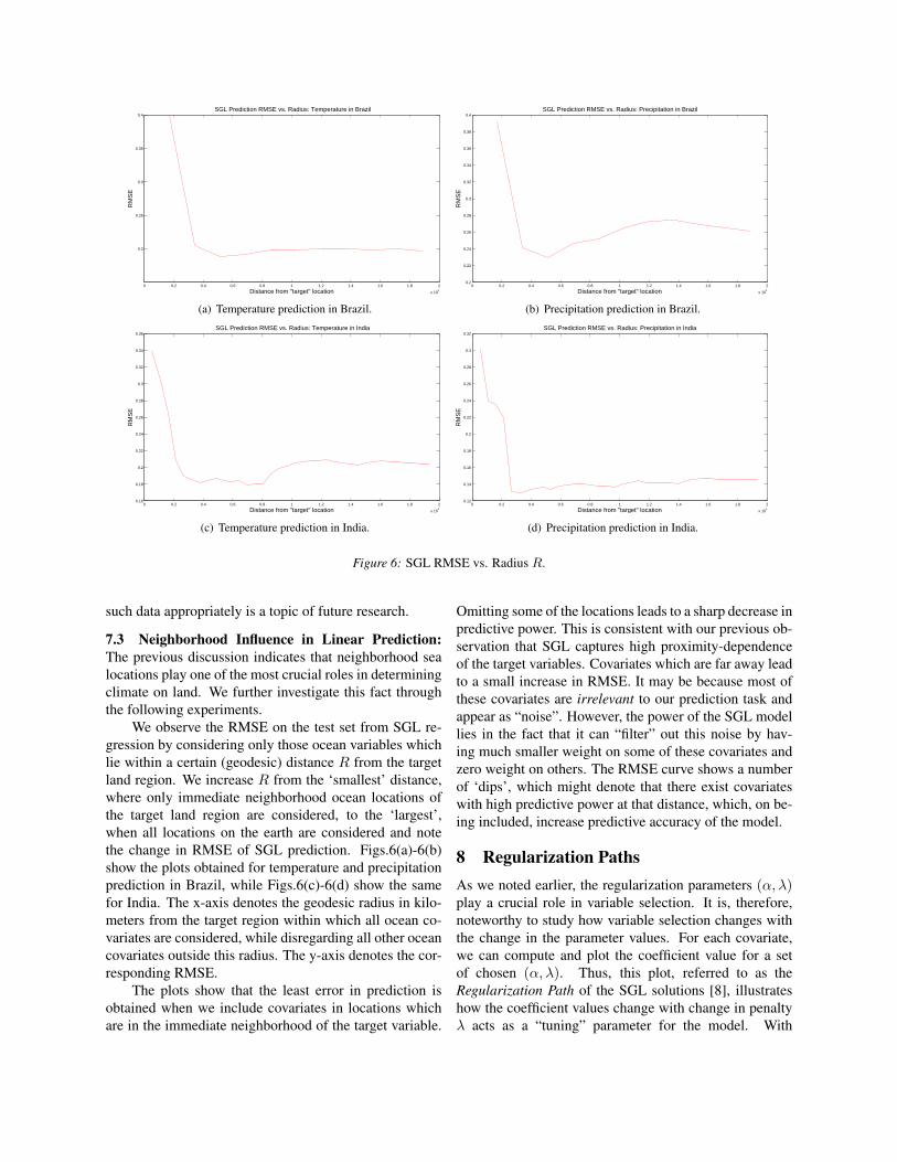
Figure 6: SGL RMSE vs. Radius R.

such data appropriately is a topic of future research.

7.3 Neighborhood Influence in Linear Prediction:The previous discussion indicates that neighborhood sealocations play one of the most crucial roles in determiningclimate on land. We further investigate this fact throughthe following experiments.

We observe the RMSE on the test set from SGL re-gression by considering only those ocean variables whichlie within a certain (geodesic) distance R from the targetland region. We increase R from the ‘smallest’ distance,where only immediate neighborhood ocean locations ofthe target land region are considered, to the ‘largest’,when all locations on the earth are considered and notethe change in RMSE of SGL prediction. Figs.6(a)-6(b)show the plots obtained for temperature and precipitationprediction in Brazil, while Figs.6(c)-6(d) show the samefor India. The x-axis denotes the geodesic radius in kilo-meters from the target region within which all ocean co-variates are considered, while disregarding all other oceancovariates outside this radius. The y-axis denotes the cor-responding RMSE.

The plots show that the least error in prediction isobtained when we include covariates in locations whichare in the immediate neighborhood of the target variable.

Omitting some of the locations leads to a sharp decrease inpredictive power. This is consistent with our previous ob-servation that SGL captures high proximity-dependenceof the target variables. Covariates which are far away leadto a small increase in RMSE. It may be because most ofthese covariates are irrelevant to our prediction task andappear as “noise”. However, the power of the SGL modellies in the fact that it can “filter” out this noise by hav-ing much smaller weight on some of these covariates andzero weight on others. The RMSE curve shows a numberof ‘dips’, which might denote that there exist covariateswith high predictive power at that distance, which, on be-ing included, increase predictive accuracy of the model.

8 Regularization PathsAs we noted earlier, the regularization parameters (α, λ)play a crucial role in variable selection. It is, therefore,noteworthy to study how variable selection changes withthe change in the parameter values. For each covariate,we can compute and plot the coefficient value for a setof chosen (α, λ). Thus, this plot, referred to as theRegularization Path of the SGL solutions [8], illustrateshow the coefficient values change with change in penaltyλ acts as a “tuning” parameter for the model. With

600 545.575 491.149 436.724 382.298 327.873 273.447 219.022 164.596 110.171 55.7455 1.32

0

0.05

0.1

0.15

0.2

0.25

0.3

0.35

0.4

λ

Coe

ffici

ent v

alue

Temperature: Brazil

Temp. off coast of Brazil

Precipitation off coast of Brazil

Figure 7: Temp. prediction in Brazil: Regularization path.

551.32 501.32 451.32 401.32 351.32 301.32 251.32 201.32 151.32 101.32 51.32 1.32

−0.05

0

0.05

0.1

0.15

0.2

0.25

0.3

0.35

λ

Coe

ffici

ent v

alue

Precipitation: Brazil

Temperature and Precipitation off coast of Brazil

Figure 8: Precip. prediction in Brazil: Regularization Path.

higher penalties, we obtain a sparser model. However, itusually corresponds to a gain in RMSE. Most importantly,though, we obtain a quantitative view of the complexity ofthe model. In particular, the covariates which persist overconsiderably large ranges of λ and α are the most robustcovariates in our regression task.

For the chosen training and test datasets, we computethe regularization path for temperature and precipitationpredictions in Brazil and India. We fix α = 0.5, so thatλ1 = λ2 = λ

2 . Figs.7 - 8 show the regularization pathsfor prediction in Brazil. The most ‘stable’ covariates,viz. temperature and precipitation in location(s) justoff the coast of Brazil, have been earlier reported asamong the most relevant covariates obtained throughcross-validation on the training set.

The regularization paths for prediction in India areplotted in Figs.9 - 10. We observe that in this casetoo, the most stable covariates are among the relevantones obtained through cross-validation. It is interestingto note that in all the plots, for low values in penalty, amild increase in penalty dramatically changes the selectedmodel. However, in higher ranges, since the only covari-ates which survive are the relevant and stable ones, thechange in model selection is more gradual.

600 545.575 491.149 436.724 382.298 327.873 273.447 219.022 164.596 110.171 55.7455 1.32

0

0.05

0.1

0.15

0.2

λ

Coe

ffici

ent v

alue

Temperature & Precipitation in Bay of Bengal

Figure 9: Temp. prediction in India: Regularization path.

600 545.575 491.149 436.724 382.298 327.873 273.447 219.022 164.596 110.171 55.7455 1.32

0

0.05

0.1

0.15

0.2

0.25

0.3

λ

Coe

ffici

ent v

alue

Temperature and Precipitation in Bay of Bengal

Figure 10: Precip. prediction in India: Regularization path.

9 ConclusionIn this paper, we have proved statistical consistency guar-antees for a general class hierarchical tree-structured normregularized estimators. It follows that SGL, which be-longs to this class, has statistical consistency of estima-tion. Application of SGL for predictive modeling of landclimate variables has shown that it inherently captures im-portant dependencies that exist between land and oceanvariables. In terms of prediction accuracy, SGL is empir-ically found to outperform the state-of-the-art models inclimate. We observe that parsimony in covariate selectionimproves predictive performance and SGL is robust in itsselection of covariates.

Hierarchical tree-structured norm regularized estima-tors provide a powerful tool for various sparse regres-sion problems in climate, such as hurricane predictionand modeling climate extremes. The results motivate usto build sparsity inducing regularizers that capture morecomplex dependency structures that are known to climatescience, e.g., ocean currents, climate cycles etc. We alsowant to incorporate temporal lags, which are known to af-fect the climate system, into our model. Our ultimate goalis to design statistical models which, when incorporatedwith the existing physical models of climate [5], can pro-vide reasonable predictions of the chaotic climate system.

Acknowledgments: This research was supported in partby NSF Grants IIS-1029711, IIS-0916750, SES-0851705,IIS-0812183, and NSF CAREER Grant IIS-0953274. Theauthors are grateful for technical support from Universityof Minnesota Supercomputing Institute (MSI).

References

[1] F. Bach, “Consistency of the group lasso and multiplekernel learning,” JMLR, vol. 9, pp. 1179–1225, 2008.

[2] P. Baldi and S. Bruna, Bioinformatics - The Machine Learn-ing Approach. MIT Press, 1998.

[3] A. Beck and M. Teboulle, “A fast iterative shrinkage-thresholding algorithm for linear inverse problems,” SIAMJournal on Imaging Sciences, vol. 2 1, pp. 183–202, 2009.

[4] E. Candes and T. Tao, “Decoding by linear programming,”IEEE Trans. on Info. Th., vol. 5112, pp. 4203–4215, 2005.

[5] CESM. Community earth system model. [Online].Available: http://www.cesm.ucar.edu/models/cesm1.0/

[6] D. P. Chambers, B. D. Tapley, and R. H. Stewart, “Anoma-lous warming in the indian ocean coincident with el nio,” J.of Geoph. Res., vol. 104, pp. 3035–3047, 1999.

[7] S. Chatterjee, “An error bound in the Sudakov-Fernique inequality,” Arxiv, Tech. Rep., 2008,http://arxiv.org/abs/math/0510424.

[8] B. Efron, T. Hastie, I. Johnstone, and R. Tibshirani, “Leastangle regression,” Ann. of Stats., vol. 32, pp. 407–499,2002.

[9] L. et. al, Ed., Intelligent Data Analysis in Medicine andPharmacology. Kluwer, 1997.

[10] L. Evers and C. Messow, “Sparse kernel methods for high-dimensional survival data,” Bioinformatics, vol. 24, no. 14,pp. 1632–1638, 2008.

[11] U. M. Fayyad, S. G. Djorgovski, and N. Weir, “Automatingthe analysis and cataloging of sky surveys,” in Advances inKnowledge Discovery and Data Mining, 1996.

[12] J. Friedman, T. Hastie, and R. Tibshirani, “A note on thegroup lasso and a sparse group lasso,” Preprint, 2010.

[13] T. Hastie, R. Tibshirani, and J. Friedman, The Elements ofStatistical Learning; Data mining, Inference and Predic-tion. Springer Verlag, New York, 2001.

[14] R. Jenatton, J. Mairal, G. Obozinski, and F. Bach, “Proxi-mal methods for sparse hierarchical dictionary learning,” inICML, June 2010, pp. 487–494.

[15] M. Ledoux and M. Talagrand, Probability in BanachSpaces: Isoperimetry and Processes. Springer, 2002.

[16] J. Liu, S. Ji, and J. Ye, SLEP: SparseLearning with Efficient Projections. [Online]. Available:http://www.public.asu.edu/∼jye02/Software/SLEP

[17] J. Liu and J. Ye, “Moreau-yosida regularization forgrouped tree structure learning,” in NIPS, 2010.

[18] NCEP/NCAR Reanalysis 1: Surface air tem-perature (0.995 sigma level). [Online]. Avail-able: http://www.esrl.noaa.gov/psd/data/gridded/data.ncep.reanalysis.surface.html

[19] S. Negahban, P. Ravikumar, M. J. Wainwright, and B. Yu,“A unified framework for high-dimensional analysis of m-

estimators with decomposable regularizers,” Arxiv, 2010,http://arxiv.org/abs/1010.2731v1.

[20] R. T. Rockafellar, Convex Analysis. Princeton UniversityPress, 1996.

[21] K. Steinhaeuser, N. Chawla, and A. Ganguly, “Comparingpredictive power in climate data: Clustering matters,” inAdvances in Spatial and Temporal Databases, vol. 6849,2011, pp. 39–55.

[22] ——, “Complex networks as a unified framework fordescriptive analysis and predictive modeling in climatescience,” Statistical Analysis and Data Mining, vol. 4, no. 5,pp. 497–511, 2011.

[23] R. Tibshirani, “Regression shrinkage and selection via thelasso,” J. Royal. Statist. Soc. B, vol. 58, pp. 267–288, 1996.

[24] A. Tsonis, G. Wang, K. Swanson, F. Rodrigues, andL. Costa, “Community structure and dynamics in climatenetworks,” Climate Dynamics, 2010.

[25] D. Watts and S. Strogatz, “Collective dynamics of small-world networks,” Nature, vol. 393, pp. 440–442, 1999.

[26] J. Wright, Y. Ma, J. Mairal, G. Sapiro, T. Huang, andS. Yan, “Sparse representation for computer vision andpattern recognition,” Proc. IEE, vol. 98, no. 6, pp. 1031–1044, 2010.

[27] M. Yuan and Y. Lin, “Model selection and estimationin regression with grouped variables,” Journal of RoyalStatistical Society Series B, vol. 68 (1), pp. 49–67, 2006.

[28] P. Zhao and B. Yu, “On model selection consistency oflasso,” JMLR, vol. 7, pp. 2541–2563, 2006.

[29] S. Zhou, J. Lafferty, and L. Wasserman, “Time varyingundirected graphs,” Machine Learning, vol. 80, pp. 295–319, 2010.