HAL Id: inria-00589204https://hal.inria.fr/inria-00589204v3

Submitted on 19 Aug 2011

HAL is a multi-disciplinary open accessarchive for the deposit and dissemination of sci-entific research documents, whether they are pub-lished or not. The documents may come fromteaching and research institutions in France orabroad, or from public or private research centers.

L’archive ouverte pluridisciplinaire HAL, estdestinée au dépôt et à la diffusion de documentsscientifiques de niveau recherche, publiés ou non,émanant des établissements d’enseignement et derecherche français ou étrangers, des laboratoirespublics ou privés.

Sparse Meshless Models of Complex Deformable SolidsFrançois Faure, Benjamin Gilles, Guillaume Bousquet, Dinesh K. Pai

To cite this version:François Faure, Benjamin Gilles, Guillaume Bousquet, Dinesh K. Pai. Sparse Meshless Models ofComplex Deformable Solids. ACM Transactions on Graphics, Association for Computing Machinery,2011, Proceedings of SIGGRAPH’2011, 30 (4), pp.Article No. 73. <10.1145/2010324.1964968>.<inria-00589204v3>

Sparse Meshless Models of Complex Deformable Solids

Francois Faure1,2,3 Benjamin Gilles4,2,3 Guillaume Bousquet1,2,3 Dinesh K. Pai51University of Grenoble 2INRIA 3LJK – CNRS 4Tecnalia 5UBC

(a) T-Bone Steak (b) Stiffness (c) Discretization (d) Compliance distance (e) Deformation

Figure 1: A taste of the method. The T-bone steak (a) has a rigid bone and softer muscle and fat, as seen in the volumetric stiffness map (b).Our method can simulate it using only three moving frames and ten integration points (c), running at 500 Hz with implicit integration on anordinary PC. The frame placement is automatically generated using a novel compliance-scaled distance (d). Observe that when one side ofthe meat is pulled (e), the bone remains rigid and the two meaty parts are correctly decoupled.

Abstract

A new method to simulate deformable objects with heterogeneousmaterial properties and complex geometries is presented. Given avolumetric map of the material properties and an arbitrary numberof control nodes, a distribution of the nodes is computed automat-ically, as well as the associated shape functions. Reference framesattached to the nodes are used to apply skeleton subspace deforma-tion across the volume of the objects. A continuum mechanics for-mulation is derived from the displacements and the material proper-ties. We introduce novel material-aware shape functions in place ofthe traditional radial basis functions used in meshless frameworks.In contrast with previous approaches, these allow coarse deforma-tion functions to efficiently resolve non-uniform stiffnesses. Com-plex models can thus be simulated at high frame rates using a smallnumber of control nodes.

CR Categories: I.3.5 [Computer Graphics]: Physically basedmodeling— [I.3.7]: Computer Graphics—Animation

Keywords: physically based animation, deformable solid, mesh-less model

Links: DL PDF

1 Introduction

Physically based deformable models have become ubiquitous incomputer graphics. So far, most of the work has focused on ob-jects made of a single, homogeneous material. However, manyreal-world objects, including biological structures such as the T-bone steak shown in Figure 1, are composed of heterogeneous ma-terial. The simulation of such complex objects using the currentlyavailable techniques requires a high resolution spatial discretiza-tion to resolve the variations of material parameters. Consequently,the realistic simulation of such complex objects has remained im-possible in interactive applications. In this paper, we address thisquestion and we propose a novel approach to the simulation of het-erogeneous, intricate materials with various stiffnesses.

The numerical simulation of continuous deformable objects isbased on a discrete number of independent degrees of freedom(DOFs) which we will call nodes in this paper. Nodes can be controlpoints, rigid frames, affine frames or any other primitive. Nodes areassociated with kernel functions or shape functions (which are sim-ilar to kernels but normalized to give a partition of unity), which arecombined to produce the displacement function of material pointsin the solid. In traditional methods, shape functions are geometri-cally designed to achieve a certain degree of locality and smooth-ness, independent of the material. The resulting deformations arerather homogeneous between the nodes. Accurately handling het-erogeneous objects requires nodes at the boundaries between thedifferent materials, and this raises well-known segmentation andmeshing issues. While a small number of smooth material discon-tinuities may be tractable, handling multiple geometrically detailedboundaries requires a dense mechanical sampling that is incompat-ible with interactive simulation. Moreover, dense sampling createsnumerical conditioning problems, especially in the case of stiff ma-terial.

In this paper, we show that it is possible to simulate complex het-erogeneous objects with sparse sampling using new, material-awareshape functions. Our approach is based on a simple observation:points connected by stiff material move more similarly than con-nected by compliant material. The limit case is the rigid body,where all points move along with one single frame. We proposea meshless framework with a moving frame attached to each node,

u

Figure 2: The displacement u of a deformable object (blue) is dis-cretized using nodes (black circles). Strain is measured based onthe deformation of local frames (black arrows) computed at inte-gration points in the material.

and we show that carefully designing the kernel functions associ-ated with the nodes allows a unification of rigid and deformablesolid mechanics. This allows the straightforward modeling of het-erogeneous objects and alleviates the meshing issues. Given a de-formable object to simulate and a number of control nodes corre-sponding to an expected computation time, optimization criteria canbe used to compute, at initialization time, a discretization of the ob-ject and the associated shape functions, in order to achieve a goodrealism.

Our specific contributions are the following: (1) a meshless simula-tion method for solids with material-aware shape functions using anovel distance function based on compliance; (2) a method to auto-matically model a complex object for this method, with an arbitrarynumber of sampling frames, based on surface meshes or volumetricdata; (3) a system that implements the above methods and showsthe ability to simulate complex deformation with a small number ofdynamic degrees of freedom.

The remainder of this paper is organized as follows. We first brieflyreview in Section 2 relevant previous work, which allows us to mo-tivate and sketch our approach with respect to the existing ones.In Section 3, we compare different types of shape functions andexplain our choice. We then study in Section 4 the problem ofmaterial-aware shape functions starting in one dimension and ex-tending to two or three dimensions, and propose a method to opti-mize the distribution of nodes. In Section 5, we derive the differen-tial equation which governs the dynamics of the object, investigateprecision issues and propose a strategy to optimize the distributionof integration points. We finally present results and discuss futurework.

2 Background and motivation

The physical simulation of deformable solids has attracted a lot ofattention in the recent decades, and a good survey can be foundin [Nealen et al. 2005]. The displacement is typically sampled ata discrete set of points, which we call nodes in this document, andit is interpolated within the object based on the nodal values, as il-lustrated in Figure 2. Elastic forces can be derived using a classicalhyperelastic scheme. Consider a material whose undeformed posi-tions p(θ) are parametrized by local, curvilinear coordinates θ (liketexture coordinates). When the material undergoes a deformation,the points are displaced to new positions p(θ) = p(θ) + u(θ), asillustrated in Figure 2. At each material point, the derivatives of theposition function p with respect to the coordinates θ are the vec-tors of a local basis, illustrated using frames in Figure 2, and theyare the columns of a 3 × 3 matrix F loosely called the deforma-tion gradient, with reference value F , typically the identity. Thelocal deformation of the material is the non-rigid part of the trans-formation F−1F between the reference and current states (like thedistortion of a checkerboard texture). The strain, ε, is a measure ofthis deformation. Different strain functions have been used, but all

of them fit in this derivation. The elastic response σ(ε) generatesthe elastic forces, and is a physical characteristic of the material. Itsproduct with the strain is homogeneous to a density of energy. Theelastic energy of a deformed object is the work done by the elas-tic forces from the undeformed state to the current state, integratedacross the whole object: W =

∫V

∫ ε0σdε. Let q be the vector of

independent DOFs of the object, responsible for the displacementsu. The associated elastic forces f are computed by differentiatingthe energy with respect to the DOFs:

fT = −∂W∂q

= −∫V

∂ε

∂qσ (1)

One additional differentiation provides us with the stiffness ∂f∂q

,used in implicit integration schemes and static solvers. Iterativelinear solvers like the conjugate gradient only address the matrixthrough its product with a vector, which amounts to computing thechange of force δ(f) corresponding to an infinitesimal change ofposition δ(q). This frees us from explicitly computing the stiffnessmatrix, and allows us to simply compute the changes of the termsin the force expression and accumulate their contributions:

δ(fT ) = −∫V∂ε∂q

∂σ∂ε

∂ε∂q

Tδ(q)

−∫V δ(

∂ε∂q

)σ(2)

The first term corresponds to the change of stress intensity. Thesecond corresponds to a change of direction due to non-linearity,and may be null or negligible, depending on the interpolation andstrain functions. Damping forces, based on velocity, can straight-forwardly be derived in this framework and added to the elasticforces.

Recently, precomputed deformation modes have been used to in-teractively deform large structures [James and Pai 2003; Barbicand James 2005; Kim and James 2009]. Using deformation modesrather than point-like nodes as DOFs allows to easily trade-off ac-curacy for speed. A layered model combining articulated bodydynamics and a reduced basis of body deformation is presentedin [Galoppo et al. 2009]. However, the deformation modes lack lo-cality and pushing on one point may deform the whole object. Ro-bustness problems such as inverted tetrahedra [Irving et al. 2006]or hourglass deformation modes in hexahedra [Nadler and Rubin2003] have been addressed. To reduce computation time, embed-ding detailed objects in coarse meshes has become popular [Mullerand Gross 2004; Sifakis et al. 2007; Nesme et al. 2009]. Discon-nected or arbitrarily-shaped elements [Kaufmann et al. 2008; Mar-tin et al. 2008] have been proposed to alleviate the meshing difficul-ties. Meshless methods, first introduced for fluid simulation, havebeen extended to solid mechanics [Muller et al. 2004; Gross andPfister 2007]. Besides continuum mechanics-based methods, fastalgorithms have been developed for video games to simulate quasi-isometry [Adams et al. 2008; Muller et al. 2005]. They are not ableto model physical properties of materials, being based on geometryonly.

Various displacement functions, strain measures and stress-strainlaws have been proposed in the literature to cope with a wide rangeof object shapes and materials, small or large displacements, andnumerical time integration methods.

In this work, we focus on the design of displacement functions.Our method is compatible with all strain measures, material param-eters and integration methods. We briefly discuss the main classesof interpolation methods previously proposed. The seminal workof Terzopoulos et al.[1987] applied finite differences in a regulargrid. In the more flexible Finite Element method [Bathe 1996], thedisplacement u is interpolated within the mesh cells (elements),as illustrated in Figure 3(a), based on cell vertices (nodes), as a

(a) (b) (c) (d)

Figure 3: Comparison of displacement functions. The black lineencloses the area where the displacement function is defined, basedon node positions (black circles) and associated functions (coloredareas). (a) Finite Element, (b) Point-based, (c) Frame-based withRBF kernels, (d) Frame-based with our material-based kernels.

weighted sum of the node displacements: p(θ) =∑i wi(θ)pi,

where the pi are the node positions, and the w are called the shapefunctions of the nodes. After years of constant progress, meshingand remeshing remains a difficult issue, see e.g. [Tournois et al.2009]. While detailed geometry can be embedded within coarsecells to reduce complexity, detailed material requires a large num-ber of cells, or complex precomputations at initialization time basedon a finer mesh [Nesme et al. 2009; Kharevych et al. 2009]. To easetopological changes, point-based (also called meshless or mesh-free) methods use radial basis functions attached to the nodes [Friesand Matthies 2003; Muller et al. 2004]. Sampling issues remain,since each interpolated point must lie in the range of at least fournon-coplanar nodes, as illustrated in Figure 3(b). A very inter-esting meshless approach using moving frames was recently pro-posed to alleviate this limitation [Martin et al. 2010], using thegeneralized moving least squares (GMLS) interpolation. In thismethod, even one single neighboring node is sufficient to com-pute a local displacement, as illustrated in Figure 3(c). Moreover,the authors introduce a new affine (first-degree) approximation ofthe strain, called elaston. In contrast with the plain (zero-degree)strain value traditionally used, this allows each integration point tocapture bending and twisting in addition to the usual stretch andshear modes. These improvements over previous methods removeall constraints on node neighborhood and allow the simulation ofobjects with arbitrary topology within a unified framework. How-ever, a dense sampling of the objects is applied, leading to highcomputation times. Modeling a T-bone steak like the one depictedin Figure 1 using the meshless methods discussed above requires alarge number of small-range nodes to prevent nodes on one side ofthe thin bone to influence the nodes on the other side. Moreover, thesimulation of the rigid part requires highly stiff interaction forceswhich may generate numerical artifacts due to poor conditioning.

Our method overcomes these limitations, while keeping the bene-fits of the frame-based meshless framework. Sparse frame-basedmodels were introduced in [Gilles et al. 2011], using skeleton sub-space deformation (SSD) across the object volume and continuummechanics to achieve physical realism. The weights are computedbased on object geometry and frame distribution, independently ofthe material parameters, but it is shown that high stiffness can besimulated using appropriate shape functions. In this article, weshow that SSD create more realistic deformations than GMLS forsparse models, and we present a new method to automatically dis-tribute the nodes and compute the shape functions based on the ma-terial property map.

3 Sparse meshless models using skinning

To model deformable objects using a small number of controlframes as discussed above, we need convenient, natural defor-mation functions. We use a generalization of the popular linear

blend skinning method or Skeleton Subspace Deformation (SSD)[Magnenat-Thalmann et al. 1988], created to embed an articulatedskeleton within a smooth deformable skin. In this section, we com-pare it with the most popular shape functions used in simulation andexplain our choice. The displacements of control nodes (i.e., theDOFs qi) are locally combined according to their shape functionwi, also called weight. The following derivations hold for differenttypes of control nodes: points, rigid frames, linearly deformable(affine) frames, and quadratic frames. Let p and p be positions inthe initial and deformed settings and u = (p− p) the correspond-ing displacement, expressed as:

u =∑i

wi(p)Aip∗ − p , (3)

where (p)∗ denotes a vector of polynomials of dimension d in thecoordinates of p and Ai(qi) is a 3× d matrix. Positions in the ref-erence, undeformed configuration are denoted using an upper bar.The matrix Ai represents the primitive transformation from its ini-tial to its current position and is straightforwardly computed basedon the independent DOFs: for instance, the 12 DOFs of an affineprimitive are directly pasted into a 3× 4 matrix, while the 6 DOFsof a rigid primitive are converted to a matrix using Rodrigues’ for-mula. For point, affine or rigid, and quadratic primitives, we re-spectively use complete polynomial bases of order n = 0, n = 1,n = 2, noted as (.)n. In 3D, we have d = (n+1)(n+2)(n+3)/6and the three first bases are: p0 = [1], p1 = [1, x, y, z]T ,p2 = [1, x, y, z, x2, y2, z2, xy, yz, zx]T . The weights constitutea partition of unity (

∑wi(p) = 1) and can be computed by nor-

malizing the kernel functions. To impose Dirichlet boundary con-ditions, it is convenient to have interpolating functions at xi, theinitial position (frame origin) of node qi in 3d space: wi(xi) = 1and wj(xi) = 0, ∀j 6= i.

Comparison with FEM and meshless methods: In finite elementmethods, the values of the shape function are typically the (gener-alized) barycentric coordinates of p within the element which con-tains the point. It is easy to show that the linear (resp. quadratic)interpolation in a tetrahedron is equivalent to linear blend skinningwith one affine (resp. quadratic) frame. Since shape functions arenot bounded by elements, linear blend skinning can achieve a moreglobal interpolation, which is more suitable with sparse DOFs.

In meshless methods, shape functions are computed based on ker-nel functions φi(‖p − xi‖). In parametric models (e.g., splines),shape functions are generally polynomial functions of material co-ordinates. However, non-linear shape functions can lead to arti-facts when modeling homogeneous materials with sparse primi-tives: in case of pure extension, a uniform deformation gradientF = dp/dp is expected, which occurs only if the shape func-tions are linear in p (i.e., dwi/dp is uniform). Contrary to lin-ear blend skinning (eq.3), the moving least squares (MLS) method[Fries and Matthies 2003] approximates the displacement by u =A(p)p∗ − p, where the 3× d blending matrix A(p) is computedat initialization time by minimizing the interpolation error at primi-tive locations. For a point p, the error is locally weighted using thekernel function: e =

∑i φi(‖p − xi‖)‖A(p)x∗i − Aix

∗i ‖2.

The least squares fit leads to the closed form solution:

u =∑i

φi(‖p− xi‖)Aix∗i x∗Ti G−1p∗ − p

G =∑i

φi(‖p− xi‖)x∗i x∗Ti (4)

Equation 4 looks very similar to the blending equation 3, except thatinitial positions p∗ are altered with a constant, non-uniform matrixused to maximize the quality of the interpolation. One drawback of

(a) (b)

(c)(d)

(e) (f)

(g)

Figure 4: Deformation modes. (a): rest shape, (b): twisting,(c),(d): compression with linear (resp. nonlinear) shape functions,(e): shear, (f): bending can be obtained using skinning, but (g): notusing GMLS with linear weights.

MLS is that G is invertible only if the point is weighted by at least dnon-coplanar nodes. To remedy this, generalized MLS has been de-veloped [Fries and Matthies 2003; Martin et al. 2010]. Contrary tolinear blend skinning, the uniformity of deformations is not ensuredin (G)MLS approaches since F is non linear in p due to the rationalfunction G−1. Moreover, using barycentric coordinates as kernelfunctions to maximize linearity, GMLS performs linear interpola-tions as illustrated in Figure 4, instead of the smooth, natural bend-ing provided by skinning. This may be sufficient with dense sam-pling, since bending can be approximated by a sequence of affinetransforms. In sparse models, the ability to simulate all the naturaldeformations between two nodes is highly desirable, which makesskinning a better choice. By combining skinning and elastons, avisually pleasing and physically sound model of a deformable solidwith stretch, shear, as well as bending and twisting, can be obtainedfrom only two frames and a single integration point.

4 Material-aware shape functions

Building sparse frame-based physical models not only requires ap-propriate deformation functions as discussed in the previous sec-tion, but also anisotropic shape functions to resolve heterogeneousmaterial as illustrated in Figure 3(d). In this section, we propose amethod to automatically compute such functions.

4.1 Compliance distance

Consider the deformation of a heterogeneous bar in one dimen-sion, as shown in Figure 5, where each point p is parameterizedby one material coordinate x. Let the endpoints p0 and p1 be thesampling points of the displacement field. At any point, the dis-placement is a weighted sum of the displacements at the samplingpoints: u(x) = w0(x)u0 + w1(x)u1. If the bar is heterogeneous,the deformation is not uniform and depends on the local stiffness,as illustrated in Figure 5(b). We call a shape function ideal if it en-codes the exact displacement within the bar given the displacementsof the endpoints, as computed by a static solution. Choosing thestatic solution as the reference is somehow arbitrary, since inertialeffects play a role in dynamics simulation. However, the computa-tion of interior positions based on boundary positions is an ill-posedproblem in dynamics, since the solution depends on the velocitiesand on the time step. Moreover, for graphics, we believe that ourperception of realism is more accurate for static scenes than whenthe object is moving. Using the static solution as a shape functionmakes sense from this point of view, and encodes more information

f

xx1

u0

u0

p1p0

u x

distance x , x10

1 0x

d c x , x10 d c x0, x1

0x 1

(a)

(b)

(c)

(d)

(e)

fu1

u1x0

Figure 5: Shape function based on compliance distance. (a): A barmade of 3 different materials, in rest state, with stiffness propor-tional to darkness. (b): The bar compressed by an external force.(c): The displacement across the bar. (d): The idealw0 shape func-tion to encode the material stiffness. (e): The same, as a functionof the compliance distance.

than a purely geometric shape function.

It is possible to derive the ideal shape functions by computing thestatic solution u(x) corresponding to a compression force f appliedto the endpoints. Note that this precomputation is exact for linearmaterials only. For simplicity, we assume that the bar has a unit sec-tion. At any point the local compression is ε = du

dx= f/E = fc,

whereE is the Young’s modulus, and its inverse c is the complianceof the material. Solving this differential equation provides us with:u(x) = u(x0) +

∫ xx0

fc dx, and since the force is constant acrossthe bar, the shape function w0 illustrated in Figure 5(d) is exactly:

w0(x) =u(x)− u(x1)

u(x0)− u(x1)=

∫ x1xc dx∫ x1

x0c dx

(5)

Let us define the compliance distance between two points a and bas: dc(a, b) =

∫ xbxac |dx|. The slope of the ideal shape function is:

dw0dx

= −c/dc(p0,p1). It is proportional to the local compliancec and to the inverse of the compliance distance between the end-points. Interestingly, the shape function is thus an affine function ofthe compliance distance, as illustrated in Figure 5(e), and it can becomputed without solving an equation.

4.2 Extension to two or three dimensions

We showed in the previous section that computing ideal shape func-tions in 1D objects, without performing compute-intensive staticanalyses as in [Nesme et al. 2009], is straightforward based on com-pliance distance. Let n be the number of points where we want tocompute exact displacements to encode in shape functions. In onedimension, both the static solution and the distance field can becomputed in linear time. In two dimensions, computing the staticsolution for n independent points requires the solution of a 2n×2nequation system. The worst case time complexity of the solution isO(n3), and direct sparse solvers can achieve it with a degree be-tween 1.5 and 2 in practice. In contrast, the computation of an

approximate distance field in a voxel grid is O(n logn), which ismuch faster, but does not allow us to expect an exact solution like inone dimension. The reason is that there is an infinity of paths fromone point to another to propagate forces across, thus the stress is notuniform and can not be factored out of the integrals and simplifiedlike in Equation 5. Another difference with the one-dimensionalcase is the number of deformation modes. Higher-dimensional ob-jects exhibit several stretching and shearing modes, and we can notexpect the ratio of displacement between two points to be the samein each mode. Since a single scalar value can not encode severaldifferent ratios, there is no ideal shape function in more than onedimension. Another limitation of this measure is that the compli-ance distance is the length (compliance) of the shortest (stiffest)path from one point to the other, independently of the other paths.Thus, two points connected by a stiff straight sliver are at the samecompliance distance as if they were embedded in a compact blockof the same material, even though they are more rigidly bound inthe latter case. Moreover, material anisotropy is not modeled usinga scalar stiffness value. Nonetheless, the compliance distance al-lows the computation of efficient shape functions, as shown in thefollowing.

4.3 Voronoi kernel functions

In meshless frameworks, each node is associated with a kernel func-tion which defines its influence in space, as presented in Section 3.A wide variety of kernel functions have been proposed in the liter-ature, most often based on spherical, ellipsoidal or parallelepipedalsupports. Our design departs from this, and is guided by a set ofproperties that we consider desirable for the simulation of sparsedeformable models. To correctly handle the example shown in Fig-ure 3d, we need to restrict kernel overlap, to prevent the influenceof the left node from unrealistically crossing the bone and reachingthe flesh on the right. We thus need to constrain the kernel values,while keeping them as smooth as possible. In particular, we favoras-linear-as possible shape functions with respect to the compli-ance distance, in order to reproduce the theoretical solution in pureextension. A kernel value should not vanish before reaching theneighboring nodes, otherwise there would be a rigid layer aroundeach node. With a sufficient number of radial basis functions, all theboundary conditions could be met [Powell 1990]. Unfortunately,shape functions computed with RBFs are generally global and canincrease with distance, producing unrealistic deformations. LocalRBFs have isotropic compact support, and are thus only approxi-mating.

Since there is no general analytical solution that can satisfy all thedesired properties, we numerically compute a discrete approximatesolution on the voxelized material property map. Solving a Laplaceor heat equation on the grid would require the solution of a largeequation system, and would compute nonlinear weight functions.

A Voronoi partition of the volume allows us to easily compute ker-nels with compact supports, imposed values and linear decrease.This can be efficiently implemented in voxelized materials usingDijkstra’s shortest path algorithm. Since a point on a Voronoi fron-tier is at equal distance from two nodes, we set the two kernel valuesto 0.5 at this point, and scale the distances accordingly inside eachcell. To extend the distance function outside a cell, we generate theisosurface of kernel value 1/4 by computing a new Voronoi sur-face between the 1/2 isosurface and the other nodes. We can thenrecursively subdivide the intervals to generate a desired number ofisosurfaces. The kernel values can straightforwardly be interpolatedbetween the isosurfaces: for instance, the value at P1 in figure 6a is( 12d3/4 + 3

4d1/2)/(d3/4 +d1/2), where di is the distance to isosur-

face of kernel value i, on Dijkstra’s shortest path the point belongsto. To compute values between the last isosurface and 0 (the neigh-

w=1/2

w=1/4

w=3/4

w=0

w=0

(a)

(b)

(c)0

1

d0d

1/4d1/2

d1

d3/4

P2

P1

Figure 6: Color map of the normalized shape function correspond-ing to the red node, computed using two Voronoi subdivisions (left),one subdivision (top right) and five subdivisions (bottom right).

boring nodes), we apply a particular scheme since points beyondthe neighbors, such as P2 in the figure, should not be influencedby the node. In this case, we linearly extrapolate the kernel func-tion: (− 1

2d1/4 + 1

4d1/2)/(d1/4 + d1/2). This technique is easily

generalized to compliance distance and all the desired propertiesare met: it correctly generates interpolating, smooth, linear and de-creasing functions between nodes. The corresponding cell shapesare not necessarily convex in Euclidean space, which allows themto resolve complex material distributions as illustrated by the com-pliance distance field in Figure 1d. Since points can be in the rangeof more than two kernels, a normalization is necessary to obtain apartition of unity and the linearity of the shape functions is not per-fectly achieved, however the functions are often close to linear asshown in the accompanying video.

When using a small number of Voronoi subdivisions, we are notguaranteed to reach all the expected regions due to inaccurate ex-trapolation (see arrow tip in Figure 6b, where d1 < 2d1/2). Increas-ing the number of isosurfaces reduces this artifact, but can lead tounrealistically large influence regions as shown in Figure 6c, wherethe right part is influenced by the red node due to the linear interpo-lation between the right and left nodes. In practice, a small numberof subdivisions are sufficient to remove noticeable artifacts whilemaintaining realistic bounds. The design of more realistic kernelsin the extreme case of a very sparse discretization, large material in-homogeneities and complex geometry, is deferred to future work.

4.4 Node distribution

The Voronoi computations provide us with a natural way to uni-formly distribute nodes in the space of compliance-scaled distances.We apply a standard farthest point sampling followed by a Lloydrelaxation (iterative repositioning of nodes in the center of theirVoronoi regions) as done in [Adams et al. 2008; Martin et al.2010]. The uniform sampling using the compliance distance re-sults in higher node density in more compliant regions, allowingmore deformation in soft regions. Since a whole rigid object cor-responds to a single point in the compliance distance metric, all itspoints in Cartesian space have the same shape function values. In-terestingly, it thus undergoes a rigid displacement, even if it is notassociated to a single node. However, due to the well-known arti-facts of linear blend skinning, it may actually undergo compressionin case of large deformations. This artifact can be easily avoided byinitializing nodes in the rigid parts, and keeping them fixed duringthe Lloyd relaxation. Another solution would be to replace linearblend skinning with dual quaternion skinning [Kavan et al. 2007],at the price of more complex mechanical computations due to nor-malization.

5 Space and time integration

This section explains how to set up the classical differential equa-tion of dynamics for our models. The simulation loop is finallysummarized in Algorithm 1.

5.1 Differential equation

We solve the classical dynamics equation

Mq− f(q, q) = fext(q, q) (6)

where M is the mass matrix, q and q are the DOF value and ratevectors, q denotes the accelerations, f the internal forces, fext theexternal and inertial forces. Without loss of generality we con-sider Implicit Euler integration (see e.g., [Baraff and Witkin 1998]),which computes velocity updates by solving the following equa-tion: (

M− hC− h2K)δq = h (fext + hKq) (7)

where h is the time step, K = ∂f∂q

is the stiffness matrix, andC = ∂f

∂qthe damping matrix, often represented using the popu-

lar Rayleigh assumption: C = αM + βK. The matrices neednot to be explicitly computed, since the popular Conjugate Gradi-ent solver addresses them only through their products with vectors.The generalized mass matrix is computed by assembling the Mij

blocks related to primitives i and j:

Mij =

∫Vρ∂u

∂qi

T ∂u

∂qj, (8)

where ρ is the mass density. For simplicity, we lump the mass ofeach primitive by neglecting the cross terms : Mij = 0, ∀i 6= j.The resulting global mass matrix is block diagonal and the Mii

are square matrices, simplifying the time integration step withoutnoticeable artifacts.

5.2 Elastic force

The computation of the elastic forces is explained in Section 2.However, we explicitly introduce the deformation gradient F in theforce computation:

fT = −∂W∂q

= −∫V

∂ε

∂qσ = −

∫V

∂ε

∂F

∂F

∂qσ (9)

This provides us with great modularity: the strain measure modulecomputes ∂ε

∂F, while the interpolation module computes ∂F

∂q, and

both can be designed and reused independently. A similar deriva-tion is used to compute the product of the stiffness matrix with avector:

δ(fT ) = −∫V∂ε∂F

∂F∂q

∂σ∂ε

∂F∂q

T ∂ε∂F

Tδ(q)

−∫V

(δ( ∂ε∂F

) ∂F∂q

+ ∂ε∂Fδ( ∂F

∂q)σ),

(10)

This modularity allows us to implement the blending of rigid, affineand quadratic primitives, and to easily combine them with a varietyof strain measures. Note that other interpolation methods, such asFEM and particle-based methods, fit in this framework. We haveimplemented the popular corotational and Green-Lagrange strains,and Hookean material laws. Incompressibility is simply handled bymeasuring the change of volume, ‖F‖ − 1, and applying a scalarresponse using the bulk modulus. Other popular models such asMooney-Rivlin and Arruda-Boyce would be easy to include.

5.3 Space integration

The quantities derived in the previous sections are numerically in-tegrated across the material using a set of function evaluations. Theaccuracy of this process, called cubature, is described by its order,meaning that polynomial functions of lower degrees can be inte-grated exactly. As discussed in section 4, linear shape functionsare desirable with sparse DOFs as they are able to generate uni-form stretching. The following table summarizes the degrees ofthe different quantities obtained with linear shape functions for dif-ferent strain measures and primitives. Classical cubature methods

Node Strain measure u M F ε, σ f

Affine/Rigid Corotational 2 4 1 1 2Affine/Rigid Green-Lagrange 2 4 1 2 4

Quadratic Corotational 3 6 2 2 4Quadratic Green-Lagrange 3 6 2 4 8

Table 1: Polynomial degrees obtained with linear shape functions.

such as the midpoint rule (order 1), the Simpson’s rule (order 3) orGauss-Legendre cubature (order 5) would require many evaluationpoints to be accurate. The most representative evaluation points canbe estimated as in [An et al. 2008], but it requires intensive staticanalysis at initialization time. Fortunately, displacements based onlinear blend skinning can be easily differentiated and all quantitiescan be integrated explicitly in regions of linear weights. In a re-gion Ve centered on p and containing points p + dp, an integratedquantity is

∫Ve v = vT

∫Ve dp

n where v is a vector containing thequantity v and its spatial derivatives up to degree n, and

∫Ve dp

n isthe integrated polynomial basis of order n over the region. This lastterm can be estimated at initialization time using the voxel maps.This integration is exact if n is the polynomial degree of v. Thisformulation generalizes the concept of elastons [Martin et al. 2010]where quantities of order n = 2 are explicitly integrated in cuboidregions. Using n = 0, the integration scheme is equivalent to themidpoint rule:

∫Ve v ≈ vVe.

The method presented in section 4 generates as-linear-as possibleshape functions. However, the gradients are discontinuous at theboundaries of the influence regions. We therefore partition the vol-ume in regions influenced by the same set of nodes, and place oneintegration sample Ve in each of them. To increase precision, werecursively subdivide the remaining regions up to the user-definednumber of integration points. Our subdivision criterion is basedon the error of a least squares fit of the voxel weights with a lin-ear function. For more precision, stiffness changes could also beconsidered.

5.4 Visual and contact surfaces

Visual and contact surfaces can be attached to the deformable ob-jects using the skinning method presented in section 3. These sur-faces can also be used to generate the voxel data, as in the exampleshown in Figure 10. The compliance distances of the vertices areinterpolated in the material volumetric map, and the shape func-tions are computed accordingly. Our framework sets no restrictionon the collision detection and response methods. Any force fp ap-plied to a point p on the contact surface can be accumulated in thecontrol nodes using the following relation, deriving from the powerconservation law:

f+ =∂p

∂q

T

fp (11)

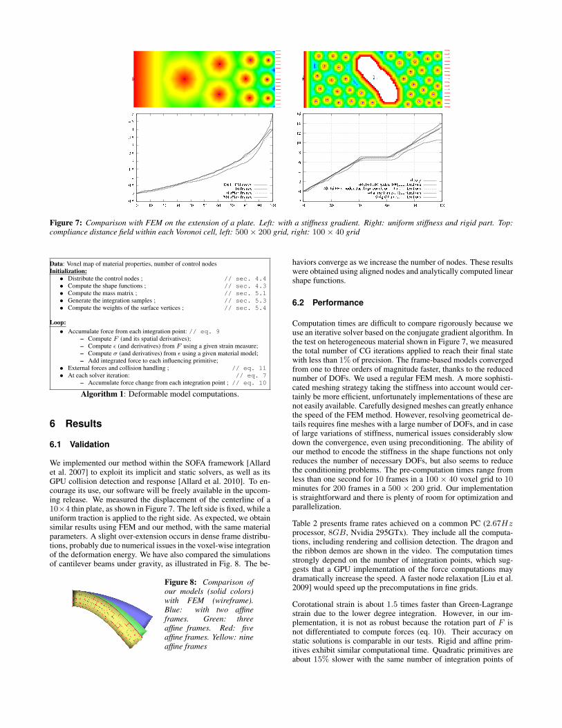
Figure 7: Comparison with FEM on the extension of a plate. Left: with a stiffness gradient. Right: uniform stiffness and rigid part. Top:compliance distance field within each Voronoi cell, left: 500× 200 grid, right: 100× 40 grid

Data: Voxel map of material properties, number of control nodesInitialization:

• Distribute the control nodes ; // sec. 4.4• Compute the shape functions ; // sec. 4.3• Compute the mass matrix ; // sec. 5.1• Generate the integration samples ; // sec. 5.3• Compute the weights of the surface vertices ; // sec. 5.4

Loop:• Accumulate force from each integration point: // eq. 9

– Compute F (and its spatial derivatives);– Compute ε (and derivatives) from F using a given strain measure;– Compute σ (and derivatives) from ε using a given material model;– Add integrated force to each influencing primitive;

• External forces and collision handling ; // eq. 11• At each solver iteration: // eq. 7

– Accumulate force change from each integration point ; // eq. 10

Algorithm 1: Deformable model computations.

6 Results

6.1 Validation

We implemented our method within the SOFA framework [Allardet al. 2007] to exploit its implicit and static solvers, as well as itsGPU collision detection and response [Allard et al. 2010]. To en-courage its use, our software will be freely available in the upcom-ing release. We measured the displacement of the centerline of a10×4 thin plate, as shown in Figure 7. The left side is fixed, while auniform traction is applied to the right side. As expected, we obtainsimilar results using FEM and our method, with the same materialparameters. A slight over-extension occurs in dense frame distribu-tions, probably due to numerical issues in the voxel-wise integrationof the deformation energy. We have also compared the simulationsof cantilever beams under gravity, as illustrated in Fig. 8. The be-

Figure 8: Comparison ofour models (solid colors)with FEM (wireframe).Blue: with two affineframes. Green: threeaffine frames. Red: fiveaffine frames. Yellow: nineaffine frames

haviors converge as we increase the number of nodes. These resultswere obtained using aligned nodes and analytically computed linearshape functions.

6.2 Performance

Computation times are difficult to compare rigorously because weuse an iterative solver based on the conjugate gradient algorithm. Inthe test on heterogeneous material shown in Figure 7, we measuredthe total number of CG iterations applied to reach their final statewith less than 1% of precision. The frame-based models convergedfrom one to three orders of magnitude faster, thanks to the reducednumber of DOFs. We used a regular FEM mesh. A more sophisti-cated meshing strategy taking the stiffness into account would cer-tainly be more efficient, unfortunately implementations of these arenot easily available. Carefully designed meshes can greatly enhancethe speed of the FEM method. However, resolving geometrical de-tails requires fine meshes with a large number of DOFs, and in caseof large variations of stiffness, numerical issues considerably slowdown the convergence, even using preconditioning. The ability ofour method to encode the stiffness in the shape functions not onlyreduces the number of necessary DOFs, but also seems to reducethe conditioning problems. The pre-computation times range fromless than one second for 10 frames in a 100 × 40 voxel grid to 10minutes for 200 frames in a 500 × 200 grid. Our implementationis straightforward and there is plenty of room for optimization andparallelization.

Table 2 presents frame rates achieved on a common PC (2.67Hzprocessor, 8GB, Nvidia 295GTx). They include all the computa-tions, including rendering and collision detection. The dragon andthe ribbon demos are shown in the video. The computation timesstrongly depend on the number of integration points, which sug-gests that a GPU implementation of the force computations maydramatically increase the speed. A faster node relaxation [Liu et al.2009] would speed up the precomputations in fine grids.

Corotational strain is about 1.5 times faster than Green-Lagrangestrain due to the lower degree integration. However, in our im-plementation, it is not as robust because the rotation part of F isnot differentiated to compute forces (eq. 10). Their accuracy onstatic solutions is comparable in our tests. Rigid and affine prim-itives exhibit similar computational time. Quadratic primitives areabout 15% slower with the same number of integration points of

Model # frames # samples # vertices # voxels tini FPSSteak 3 10 5k 67k 3s 500Steak 10 53 5k 67k 8s 100Steak 20 140 5k 67k 12s 40

Dragon 3 6 20k 7M 100s 300Dragon 10 41 20k 7M 220s 150Dragon 20 158 20k 7M 360s 27Ribbon 5 9 4k 60k 4s 200Knee 10 200 35k 500k 11s 10Rat 30 230 600k 1.5M 90s 8

Table 2: Timings.

Figure 9: The flesh and the fat, although interpolated between thesame two control frames, pulled at the black point, exhibit differentstrains due to different stiffnesses.

the same degree. We believe that the best compromise between ac-curacy and performance is achieved using affine primitives: theyhave more DOFs than rigid frames so can capture more deforma-tion modes, and they require significantly fewer integration pointsthan quadratic primitives if we limit the expansion of the defor-mation gradient to the first order, and the integration degree to 4(= 30 polynomial terms). In theory, quadratic primitives wouldneed a second order expansion of F and an 8th order integration(= 165 polynomial terms), which would be more costly. Affine andrigid frames require only one integration point per region with lin-ear shape function, providing the main deformation modes of a rodusing only two frames and one integration point (see Figure 4). Inour implementation, linear blend skinning of rigid frames is aboutfive times faster than dual quaternion skinning [Gilles et al. 2011]with the same number of integration points. Dual quaternion skin-ning is more accurate in large bending (no volume loss) but requiresmore integration points due to the non-linear blending function andis significantly more complex to implement.

We found that sampling integration points in the overlapping influ-ence regions was a suitable strategy, since it allowed a good lin-ear approximation of the fine grained shape function defined in thevoxel grid: in our test, the average difference was 0.05 (the shapefunction being defined between 0 and 1, making the approximationerror less than 5%). This result also shows that the normalization ofthe kernel function does not significantly change the linearity. Uni-formly distributed sample points unrealistically increase the stiff-ness because soft parts are assigned with a high stiffness due toaveraging in the sample region.

6.3 Simulations

Figure 9 shows a close-up of the high speed simulation presentedin Figure 1, which runs at haptic rates. The fat undergoes more de-formation than the flesh because it is more compliant, even thoughthey are interpolated between the two same control frames. Themethod of [Nesme et al. 2009] also realistically resolves hetero-geneous materials, but a rigid bone across several elements wouldresult in high stiffnesses and generate numerical problems. In con-trast, our method handles the rigid parts straightforwardly, indepen-dently of their shape.

Our method allows the interactive simulation of complex biologicalsystems such as the knee joint shown in Figure 10. In this model,

Figure 10: Interactive knee simulation using 10 nodes. Pulling thequadriceps lifts the tibia.

Figure 11: Mix of animation and simulation. Top: the completemodel. Bottom left: model subset animated using motion capture.Bottom right: result, with flesh and tail animated using physics.

we have integrated four different tissues: bones, muscles, fat andligaments. With only 10 nodes, we are able to realistically simu-late flexion and fine movements such as the motion of the patella(knee cap) at 10 frames per second, without any prior knowledgeof the kinematic skeleton. Forces are transmitted from the quadri-ceps to the tibia suggesting that accurate dynamic models of theanatomy, taking into account muscle actuation, could be built. Afew modifications in the voxelization and material modules wouldallow motion discontinuity between tissues in contact and a moreaccurate simulation of the highly anisotropic non-linear fibrous bi-ological tissues.

Our method can also be used to easily simulate physically-basedsecondary motions from skeleton-based animation or motion cap-ture, as illustrated in Figure 11. The skin and the complete skeletonof a rat were acquired from micro-CT data. We applied our methodto automatically sample the intermediate soft tissues and the tailwith additional nodes. Optical motion capture was used to cap-ture the movements of the limbs, head and three bones on the back.Real-time interaction with the soft tissues such as the belly and thetail is shown in the accompanying video.

7 Conclusion

We have introduced novel, anisotropic kernel functions using a newdefinition of distance based on compliance, which allow the encod-ing of detailed stiffness maps in coarse meshless models. Theycan be combined with the popular skinning deformation methodto straightforwardly simulate large, physically sound deformationsof complex heterogeneous objects, using small numbers of controlnodes and small computation times. In contrast with classical FEM

and with the methods using geometrical shape functions, our ap-proach decouples the resolution of the material from the resolutionof the displacement function. The ability of setting an arbitrarilylow number of frames, combined with a compliance-based distribu-tion strategy, allows fast models to capture the most relevant defor-mation modes. In future work, we plan to investigate the dynamicadaptivity of the models allowed by the low pre-processing timeof the method. Since sparse DOFs are not able to produce localdeformations contrary to dense method such as FEM and GMLS,accuracy could be improved by refining contact regions on-the-fly.

Acknowledgements

We would like to thank Laurence Boissieux and Francois Jourdesfor models, Estelle Duveau and Lionel Reveret for the rat data.This work is partly funded by European project PASSPORT forLiver Surgery (ICT-2007.5.3 223894) and French ANR project So-HuSim. Thanks to the support of the Canada Research Chairs Pro-gram, NSERC, CIHR, Human Frontier Science Program, and PeterWall Institute for Advanced Studies.

References

ADAMS, B., OVSJANIKOV, M., WAND, M., SEIDEL, H.-P., ANDGUIBAS, L. 2008. Meshless modeling of deformable shapes andtheir motion. In Symposium on Computer Animation, 77–86.

ALLARD, J., COTIN, S., FAURE, F., BENSOUSSAN, P.-J.,POYER, F., DURIEZ, C., DELINGETTE, H., AND GRISONI, L.2007. SOFA - an open source framework for medical simulation.In Medicine Meets Virtual Reality, MMVR 15, 2007, 1–6.

ALLARD, J., FAURE, F., COURTECUISSE, H., FALIPOU, F.,DURIEZ, C., AND KRY, P. 2010. Volume contact constraintsat arbitrary resolution. ACM Transactions on Graphics 29, 3.

AN, S. S., KIM, T., AND JAMES, D. L. 2008. Optimizing cubaturefor efficient integration of subspace deformations. ACM Trans.Graph. 27, 5, 1–10.

BARAFF, D., AND WITKIN, A. 1998. Large steps in cloth simula-tion. SIGGRAPH Comput. Graph. 32, 106–117.

BARBIC, J., AND JAMES, D. L. 2005. Real-time subspace integra-tion for St. Venant-Kirchhoff deformable models. ACM Trans-actions on Graphics (SIGGRAPH 2005) 24, 3 (Aug.), 982–990.

BATHE, K. 1996. Finite Element Procedures. Prentice Hall.

FRIES, T.-P., AND MATTHIES, H. 2003. Classification andoverview of meshfree methods. Tech. rep., TU Brunswick, Ger-many.

GALOPPO, N., OTADUY, M. A., MOSS, W., SEWALL, J., CUR-TIS, S., AND LIN, M. C. 2009. Controlling deformable materialwith dynamic morph targets. In Proc. of the ACM SIGGRAPHSymposium on Interactive 3D Graphics and Games.

GILLES, B., BOUSQUET, G., FAURE, F., AND PAI, D. 2011.Frame-based elastic models. ACM Transactions on Graphics.

GROSS, M., AND PFISTER, H. 2007. Point-Based Graphics. Mor-gan Kaufmann.

IRVING, G., TERAN, J., AND FEDKIW, R. 2006. Tetrahedral andhexahedral invertible finite elements. Graph. Models 68, 2.

JAMES, D. L., AND PAI, D. K. 2003. Multiresolution green’s func-tion methods for interactive simulation of large-scale elastostaticobjects. ACM Trans. Graph. 22 (January), 47–82.

KAUFMANN, P., MARTIN, S., BOTSCH, M., AND GROSS, M.2008. Flexible simulation of deformable models using discon-tinuous galerkin fem. In Symposium on Computer Animation.

KAVAN, COLLINS, ZARA, AND O’SULLIVAN. 2007. Skinningwith dual quaternions. In Symposium on Interactive 3D graphicsand games, 39–46.

KHAREVYCH, L., MULLEN, P., OWHADI, H., AND DESBRUN,M. 2009. Numerical coarsening of inhomogeneous elastic ma-terials. ACM Trans. Graph. 28 (July), 51:1–51:8.

KIM, T., AND JAMES, D. L. 2009. Skipping steps in deformablesimulation with online model reduction. ACM Trans. Graph. 28(December), 123:1–123:9.

LIU, Y., WANG, W., LEVY, B., SUN, F., YAN, D.-M., LU, L.,AND YANG, C. 2009. On Centroidal Voronoi TessellationEn-ergy Smoothness and Fast Computation. ACM Trans. Graph. 28(08).

MAGNENAT-THALMANN, N., LAPERRIERE, R., AND THAL-MANN, D. 1988. Joint dependent local deformations for handanimation and object grasping. In Graphics interface, 26–33.

MARTIN, S., KAUFMANN, P., BOTSCH, M., WICKE, M., ANDGROSS, M. 2008. Polyhedral finite elements using harmonicbasis functions. Comput. Graph. Forum 27, 5.

MARTIN, S., KAUFMANN, P., BOTSCH, M., GRINSPUN, E., ANDGROSS, M. 2010. Unified simulation of elastic rods, shells, andsolids. SIGGRAPH Comput. Graph. 29, 3.

MULLER, M., AND GROSS, M. 2004. Interactive virtual materials.In Graphics Interface.

MULLER, M., KEISER, R., NEALEN, A., PAULY, M., GROSS,M., AND ALEXA, M. 2004. Point based animation of elastic,plastic and melting objects. In Symposium on Computer Anima-tion, 141–151.

MULLER, M., HEIDELBERGER, B., TESCHNER, M., ANDGROSS, M. 2005. Meshless deformations based on shapematching. ACM Transactions on Graphics 24, 3, 471–478.

NADLER, B., AND RUBIN, M. 2003. A new 3-d finite element fornonlinear elasticity using the theory of a cosserat point. Int. J. ofSolids and Struct. 40, 4585–4614.

NEALEN, A., MULLER, M., KEISER, R., BOXERMAN, E., ANDCARLSON, M. 2005. Physically based deformable models incomputer graphics. In Comput. Graph. Forum, vol. 25 (4), 809–836.

NESME, M., KRY, P., JERABKOVA, L., AND FAURE, F. 2009.Preserving Topology and Elasticity for Embedded DeformableModels. SIGGRAPH Comput. Graph..

POWELL, M. J. D. 1990. The theory of radial basis function ap-proximation. University Numerical Analysis Report.

SIFAKIS, E., DER, K. G., AND FEDKIW, R. 2007. Arbitrarycutting of deformable tetrahedralized objects. In Symposium onComputer Animation.

TERZOPOULOS, D., PLATT, J., BARR, A., AND FLEISCHER, K.1987. Elastically deformable models. In SIGGRAPH Comput.Graph., M. C. Stone, Ed., vol. 21, 205–214.

TOURNOIS, J., WORMSER, C., ALLIEZ, P., AND DESBRUN, M.2009. Interleaving delaunay refinement and optimization forpractical isotropic tetrahedron mesh generation. ACM Trans.Graph. 28 (July), 75:1–75:9.