7

December 2016 IEEE Information Theory Society Newsletter

Sparse Regression CodesRamji Venkataramanan, University of Cambridge, ramji.v@eng.cam.ac.uk

Sekhar Tatikonda, Yale University, sekhar.tatikonda@yale.edu Andrew Barron, Yale University, andrew.barron@yale.edu

1. IntroductionDeveloping computationally-efficient codes that approach the Shannon-theoretic limits for communication and compression has long been one of the major goals of information and coding theory. There have been significant advances towards this goal in the last couple of decades, with the emergence of turbo and sparse-graph codes in the ‘90s [1, 2], and more recently polar codes and spa-tially-coupled LDPC codes [3–5]. These codes are all primarily for discrete-alphabet sources and channels.

There are many channels and sources of practical interest where the alphabet is inherently continuous, e.g., additive white Gauss-ian noise (AWGN) channels, and Gaussian sources. A promising class of codes for Gaussian models is the recently proposed Sparse Superposition Codes or Sparse Regression Codes (SPARCs). This arti-cle provides a broad overview of SPARCs, covering theory, algo-rithms, and some practical implementation aspects. At the end, we discuss some open problems and future directions for research.

This survey is based on the tutorial on sparse regression codes pre-sented at ISIT ‘161. The discussion will be relatively informal. We paraphrase some of the technical results with the aim of provid-ing intuition, and point the reader to references for an in-depth discussion.

To motivate the construction of SPARCs, let us begin with the standard AWGN channel with signal-to-noise ratio denoted by snr. The goal is to construct codes with computationally efficient encoding and decoding that provably achieve the channel capacity

( ) log1 2 1 snrC = +^ h bits/transmission. In particular, we are in-terested in codes whose encoding and decoding complexity grows no faster than a low-order polynomial in the block length n.

Though it is well known that rates approaching C can be achieved with Gaussian codebooks, this has been largely avoided in prac-tice due to the high decoding complexity of unstructured Gauss-ian codes. Instead, the popular approach has been to separate the design of the coding scheme into two steps: coding and modula-tion. State-of-the-art coding schemes for the AWGN channel such as coded modulation [6–8] use this two-step design, and combine binary error-correcting codes such as LDPC and turbo codes with standard modulation schemes such as Quadrature Amplitude Modulation (QAM). Though such schemes have good empirical performance, they have not been proven to be capacity-achieving for the AWGN channel.

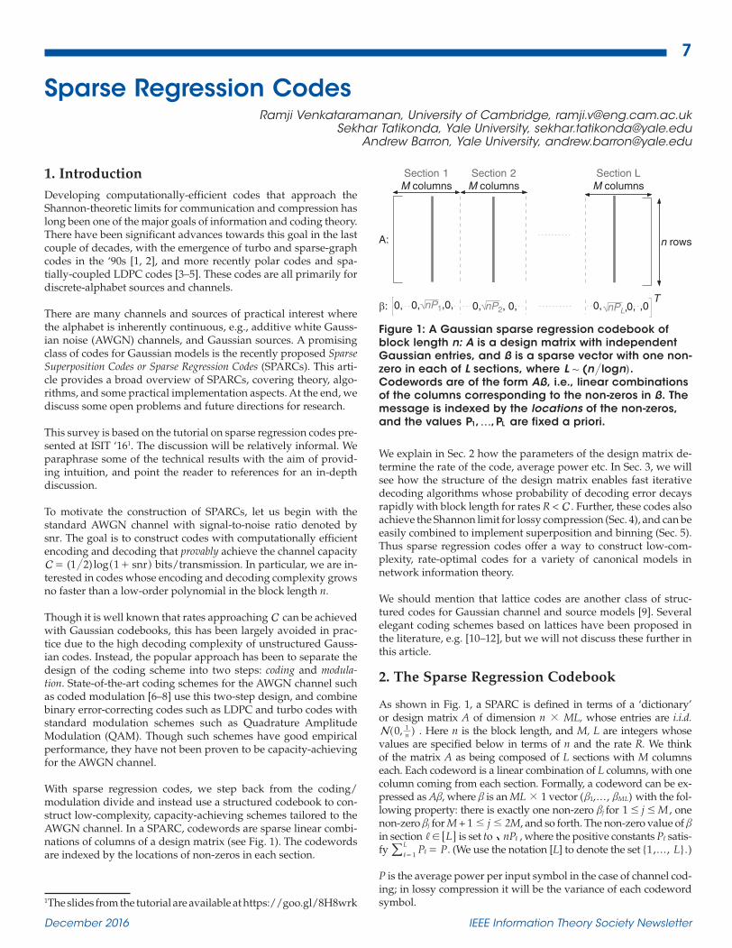
With sparse regression codes, we step back from the coding/modulation divide and instead use a structured codebook to con-struct low-complexity, capacity-achieving schemes tailored to the AWGN channel. In a SPARC, codewords are sparse linear combi-nations of columns of a design matrix (see Fig. 1). The codewords are indexed by the locations of non-zeros in each section.

1The slides from the tutorial are available at https://goo.gl/8H8wrk

We explain in Sec. 2 how the parameters of the design matrix de-termine the rate of the code, average power etc. In Sec. 3, we will see how the structure of the design matrix enables fast iterative decoding algorithms whose probability of decoding error decays rapidly with block length for rates R < C . Further, these codes also achieve the Shannon limit for lossy compression (Sec. 4), and can be easily combined to implement superposition and binning (Sec. 5). Thus sparse regression codes offer a way to construct low-com-plexity, rate-optimal codes for a variety of canonical models in network information theory.

We should mention that lattice codes are another class of struc-tured codes for Gaussian channel and source models [9]. Several elegant coding schemes based on lattices have been proposed in the literature, e.g. [10–12], but we will not discuss these further in this article.

2. The Sparse Regression Codebook

As shown in Fig. 1, a SPARC is defined in terms of a ‘dictionary’ or design matrix A of dimension n # ML, whose entries are i.i.d.

,0N n1^ h . Here n is the block length, and M, L are integers whose

values are specified below in terms of n and the rate R. We think of the matrix A as being composed of L sections with M columns each. Each codeword is a linear combination of L columns, with one column coming from each section. Formally, a codeword can be ex-pressed as Ab, where b is an ML # 1 vector (b1,..., bML) with the fol-lowing property: there is exactly one non-zero bj for j M1 # # , one non-zero bj for M + 1 # j # 2M, and so forth. The non-zero value of b in section L, ! 6 @ is set to nP, , where the positive constants Pℓ satis-fy P PL

1 =,,=/ . (We use the notation [L] to denote the set {1,..., L}.)

P is the average power per input symbol in the case of channel cod-ing; in lossy compression it will be the variance of each codeword symbol.

Figure 1: A Gaussian sparse regression codebook of block length n: A is a design matrix with independent Gaussian entries, and ß is a sparse vector with one non-zero in each of L sections, where log( nL n )+ . Codewords are of the form Aß, i.e., linear combinations of the columns corresponding to the non-zeros in ß. The message is indexed by the locations of the non-zeros, and the values , ,P P1 Lf are fixed a priori.

A:

β: 0,√nP2, 0, √nPL,0, ,00,

Section 1M columns

Section 2M columns

Section LM columns

T

n rows

0,√nP1,0, 0,

8

IEEE Information Theory Society Newsletter December 2016

Since each of the L sections contains M columns, the total number of codewords is ML. To obtain a rate R code, we need

.logM L M nR2 orL nR= = (1)

(Throughout, we use log for logarithm with base 2, and ln for base e.) There are several choices for the pair (M ,L) which satisfy (1). For example, L = 1 and M = 2nR recovers the Shannon-style random codebook in which the number of columns in A is 2nR. For our con-structions, we will choose M equal to La, for some constant a > 0. In this case, (1) becomes

a .logL L nR= (2)

Thus logL n nH= ^ h , and the size of the design matrix A (given by n # ML = n # La+1) grows polynomially in n. In our numerical simulations, typical values for L are 512 or 1024.

We note that the SPARC is a non-linear code with pairwise de-pendent codewords. Two codewords Ab and Abl are dependent whenever the underlying message vectors b,blshare one or more common non-zero entries.

Power Allocation: The coefficients P L1, ,=" , , plays an important role

in determining the performance of the code, both for channel cod-ing and for lossy compression. We will consider allocations where

LP 1l H= ^ h. Two examples are:

Flat power allocation across sections: ,PLP L, !=, 6 @.

Exponentially decaying power allocation: Fix parameter l > 0. Then ,P L2 /L ,? !,

,l- 6 @.In Section 3, we discuss computationally efficient decoders which asymptotically achieve capacity with the exponentially decay-ing allocation (with l = 2C). To improve decoding performance at practical block lengths, we explore different power allocation strategies in Section 3.3, and demonstrate that judicious power allocation can lead to dramatic improvements in decoding per-formance at finite block lengths. We also describe how decoding complexity can be reduced by replacing the Gaussian design ma-trix with a Hadamard-based design.

3. AWGN Channel Coding with SPARCs

The channel is described by the model

, , , .y x w i n1i i i f= + = (3)

The noise variables wi are i.i.d. ,0N 2+ v^ h. There is an average power constraint P on the input: the codeword : , ,x x xn1 f= ^ h should satisfy x Pn ii

1 21 #=/ . The signal-to-noise ratio P 2v is

denoted by snr.

Encoding: The encoder splits its stream of input bits into segments of log M bits each. A length ML message vector b0 is indexed by L such segments – the decimal equivalent of segment ℓ determines the position of the non-zero coefficient in section ℓ of b0. The input codeword is then computed as x A 0b= . Note that computing x simply involves adding L columns of A, weighted by the appro-priate coefficients.

Optimal Decoding: Assuming that the codewords are equally like-ly, the optimal decoder produces

,argmin y Aopt2

b b= -b

t tt

where : , ,y y yn1 f= ^ h, and the minimum is over all the message vectors in the codebook.

Probability of Error: The performance of a SPARC decoder is measured by the section error rate, which is the fraction of sec-tions decoded wrongly. The section error rate is denoted by

: 1Esec LL1

01 !b b= , ,,=t" ,/ . For a given decoder, we will aim to

bound the probability of the event Esec2 e" , for 02e . Assum-ing that the mapping determining the non-zero location for each segment of log M input bits is generated uniformly at random, a section error will, on average, lead to half the bits correspond-ing to the section being decoded wrongly. Therefore, when a large number of segments are transmitted, the bit error rate of a SPARC decoder will be close to half its section error rate.

If we want the decoding error probability of the message b0 to be small, we can use a concatenated code with the SPARC as the in-ner code and an outer Reed-Solomon (RS) code. (An RS code of rate (1 − 2e) can correct upto a fraction e of section errors in the SPARC; see [13] for details.)

We will not consider the outer RS code in the remainder of this article, and focus mostly on the section error rate (or bit error rate) of the SPARC.

Performance with Optimal Decoding: For rates R < C , the least-squares decoder was shown in [13] to have error probabili-ty decaying exponentially in the block length.

Theorem 1. [13] Consider a SPARC with rate R < C , block length n, and equal power allocation, i.e, ,P LP L, !=, ^ h 6 @. For any e > 0, the sec-tion error rate of the least-squares decoder satisfies

( ) .KeP E { ,( ) }sec

minn C R 2

2 #e l e- -

where l, K are universal positive constants.

This result was extended to SPARCs with i.i.d. binary (!1) de-sign matrices in [14, 15]. The exponent l in Theorem 1 is smaller than the Shannon-Gallager random coding exponent, but the re-sult shows that SPARCs are essentially as good as Shannon-style random codes for the AWGN channel with maximum-likelihood decoding.

3.1. Feasible SPARC Decoders

In contrast to the least-squares decoder, the feasible decoders we discuss all use a decaying power allocation across sections. Think-ing of the L sections of a SPARC as analogous to L users sharing a Gaussian multiple- access channel (MAC), leads to an exponen-tially decaying power allocation of the form ,P L2 /C L2 ,? !,

,- 6 @. Indeed, consider the equal-rate point on the capacity region of a L-user Gaussian MAC where each user gets rate C/L. It is well-known [16, 17] that this rate point can be achieved with the above power allocation via successive cancellation decoding, where user 1 is first decoded, then user 2 is decoded after subtracting the codeword of user 1, and so on.

9

December 2016 IEEE Information Theory Society Newsletter

However, successive cancellation performs poorly for SPARC de-coding. This is because L, the number of sections (“users”) in the codebook, grows as / logn n , while M, the number of codewords per user, only grows polynomially in n. An error in decoding one section affects the decoding of future sections, leading to a large number of section errors after L steps.

The first feasible SPARC decoder, proposed in [18], controls the ac-cumulation of section errors using adaptive successive decoding. The idea is to not pre-specify the order in which sections are decoded, but to look across all the undecoded sections in each step, and adap-tively decode columns which have a large inner product with the re-sidual. The main ingredients of the algorithm are as follows. In the first step, the decoder computes the inner product of each column of the design matrix with the normalized channel output sequence

/y y , and picks those columns for which this test statistic exceeds a pre-specified threshold; this gives the first estimate 1bt . In the second step, the test statistic is generated based on the residual r y A1 1b= - t

: the decoder picks the columns (from the as yet undecoded sections) whose inner product with /r r1 1 crosses the threshold; this gives

2bt . The algorithm continues in this fashion, decoding columns using the residual-based statistics in each step. The algorithm is run for a pre-specified number of steps, arranged to be of the order of log M; it terminates earlier if at least one column has been selected from each section, or the test-statistics in any step are all below the threshold.

The performance of this decoder was analyzed in [18]. With power allocation P 2 /C L2?, ,- , it was shown that the probability of message decoding error decays as ( ( ) )exp kL C RM

2- , where C C 1 log

cM M= -^ h for a constant c > 0, and R is the total rate

(SPARC combined with an outer Reed-Solomon code).

Therefore the adaptive successive threshold decoder is capacity-achieving, and the gap to capacity is of order log M1 . However, in practice, the section error rates at practically feasible block lengths are observed to be rather high for rates near capacity. The following two decoders improve the decoding performance by avoiding hard decisions about which columns to decode in each step.

3.2. Iterative Soft-decision Decoding

The key idea in the next two decoders is to iteratively update the posterior probabilities of each entry of b being the true non-zero in its section. The goal in both decoders is to iteratively generate test statistics that (in step t) have the form Zstatt t t. b x+ , where Zt is standard normal and independent of b. In words, statt is es-sentially the message vector observed in independent additive Gaussian noise with known variance t

2x . Assuming this is true, the Bayes-optimal estimate for b in the next step is

( tat ) [ | stat ] (stat ),s ZEt t tt

t t t1b b b x h= + = =+

where the conditional expectation t $h ^ h can be computed using the known prior on b (locations of non-zeros uniformly distrib-uted within each section). For indices j in section ℓ of beta, we have

:/

/, , .

expexp

secs nPnP s

nP sj Ltion,

sec

t jk tk

j t

2

2

, ,! !hx

x= ,

,

,

! ,

^ ^^h h

h 6 @/ (4)

Note that /s nP,t jh ,^ h is the posterior probability (given statt) that term j is the non-zero coefficient in section ℓ of b.

In addition to statt having the desired distributional representati-on, we also want t

2x , the variance of the noise in the test statistic, to be computable iteratively from t 1

2x - as follows. Starting with P0

2 2x v= + , we define

|

,

nZ

nZ

1

1

E E

E

t t t

t t t

2 21 1

2

21 1

2

x v b b b x

v b h b x

= + - +

= + - +

- -

- -^ h6

@@

(5)

where the expectation on the right is over b and the indepen-dent standard normal vector Zt. In other words, we want the noise in the test statistic to have two independent Gaussian components: one component with variance v2 arising from the channel noise, and the other component arising from the er-ror in the current estimate bt. The recursion to generate t

2x from t 12x - can be written as

P x1t t2 2

1x v x= + - -^ ^ hh (6)

where :x xt t 1x= -^ h is an expectation of a function of ML standard normal random variables. The exact formula for x t 1x -^ h can be found in [19, Sec. 3]. Compact asymptotic formulas for xt, t

2x are given in Lemma 1 below.

Therefore, under the assumed distribution for statt, we have ( )P x1En

tt

1 2< <b b- = - ; it can also be shown that PxE En n

T t tt

1 1 2b b b= =6 @ [19, Prop. 3.1]. Thus the scalar xt can be interpreted as the expected (power-weighted) success rate, and

( )P x1 t- as the expected interference contribution to the noise variance

t2x due to the undecoded sections. With this interpreta-

tion, for succesful decoding we want xt to be very close to 1 when the algorithm terminates. Indeed, it can be verified that for all rates less than C and P 2 /C L2?, ,- , the iteration (6) has a fixed point with t

2x close to v2, i.e., xt is close to one. A more precise version of this statement in the large system limit is given in Lemma 1 below.

Finally, the key question is: how do we iteratively generate sta-tistics statt that in each step are well-approximated as Zt tb x+ , with

t2x having the representation described above? The two de-

coders described below achieve this via seemingly very different approaches.

Adaptive Successive Soft-Decision Decoder [20–22]

The statistics for this decoder are defined using the fits : , : , , :Y A AFit Fit Fitt

t0 1

1 fb b= = = . With G0 := Y, recursively de-fine Gt to be the part of Fitt that is orthogonal to , , ,G G Gt0 1 1f - . The ingredients of statt are the vectors , ,Z Zt0 f , defined as

, .nG

A G k 0Zkk

Tk $=

The test statistic is then defined as stat Zt t k

t

k kt

0x bm= +=/ . The

weights km have to be carefully chosen in order for statt to be close enough in distribution to the desired form Zt tb x+ . The estimate bt+1 is generated as statt th ^ h, where t $h ^ h is given by (4).

Two different ways to choose the weights km , k t0 # # , are pro-posed in [21, 22]. Each of these choices is based on a technical lemma [20, Lemma 1] characterizing the distribution of Zk , k6 . The first choice of weights is deterministic, and given by

: , , , ,, , , 1 1 1 1 1t t

t t0 1

0 12

02 2

12ff x

x x x x xm mm - - - -

-

^ ch m (7)

10

IEEE Information Theory Society Newsletter December 2016

where , , t0 fx x are given by (5 ) . The analysis in [21] shows that this choice of weights makes statt close to the desired representation Zt tb x+ , leading to the following concentra-tion result.

Theorem 2. [21, Lemma 7] Consider a SPARC with rate R < C, param-eters (n, L, M) chosen according to (1), and power allocation P 2 /C L2?, ,-

. For t $ 1, let

: .nP x nP x1 1AtT t

tt

t2

,2 2f eb b b= - - h$ $. .

Then, we have

,explog

a kMnP Ak

tk k k

k

t

1 2 12

1, K e-= +

=c ^ h m" , /

where k , a 1, . . . , a t are universal constants depending on R,C.

The probability bound on the event At in Theorem 2 can be shown to imply a probability bound for the section-error rate exceeding cf, where c > 0 is a constant. Thus the probability of decoding fail-ure decays exponentially in / logn n T2 1*+^ h , where T* is the number of steps for which the algorithm is run. This is in contrast to the optimal decoder in Theorem 1 whose probability of decoding fail-ure decays exponentially in n.

As an alternative to the deterministic weights in (7), weights {m k} depending on the channel output y were also proposed in [21]. This choice is based on the Cholesky decomposition of a matrix generated from the estimates {b1, . . . , bt}. A performance guaran-tee similar to Theorem 2 can be obtained for this set of weights as well; see [21, 22] for details.

Approximate Message Passing Decoder [19, 23]

Approximate message passing (AMP) refers to a class of algo-rithms [24–30] that are Gaussian or quadratic approximations of loopy belief propagation algorithms (e.g., min-sum, sum-product) on dense factor graphs. In its basic form [24, 27], AMP gives a fast iterative algorithm to solve the LASSO, i.e., to compute

,arg min y ALASSO 22

1b b bm= - +b

t t tt

for any m > 0. Recall that the decoding problem we wish to solve is

arg min y ASPARC 22

b b= -b

t tt

over bt that are valid SPARC code-words.

One cannot directly use the LASSO-AMP of [24, 27] for SPARC decoding as it does not use the prior knowledge about b, i.e., the knowledge that b has exactly one non-zero value in each section, with the values of the non-zeros also being known.

An AMP decoder for SPARCs can be derived by writing down min-sum like updates for the SPARC decoding problem, and then approximating them using the recipe in [26]. This leads to a de-coder with the following update rules [19]. Define r0 = y, and for t $ 1 compute:

,r y A r Pn

t t

t

t t

12

1 2

bx

b= - + -

-

- c m ,A rstatt

T t tb= +

.stattt t

1b h=+ ^ h

The coefficients t2x are recursively defined by (6), starting with

P02 2x v= + . Following the terminology in [24, 26], we refer to this

recursion as state evolution (SE). Recall that the SE equations are derived under the assumption that statt is distributed as Zt tb x+ . The presence of the “Onsager” term r Pt

t n1

12 2t

x -b-

- ` j in the de-finition of the modified residual rt is crucial to ensure that the dis-tributional assumption is valid, at least asymptotically. Intuition about role of the Onsager term in the standard AMP algorithm can be found in [26, Section I-C].

We can derive a compact asymptotic formula for the SE recursion by taking the limit as L, M, n " 3 while satisfying (1). (This limit is denoted below by ‘lim’.)

Lemma 1. [19] For t $ 1, the asymptotic value of t2x , denoted by t

2x , is given by

,P x1t t2 2

1x v x= + - -r r^ ^ hh

where the function x $r ^ h is defined as follows. With :c LP=, , , we have

: .lim lim lim lnx xPP c R1 2 2

L

1

22x x x= = ,

,

,

=

r ^ ^ ^h h h" ,/

Recalling that xt+1 is the expected power-weighted fraction of cor-rectly decoded sections after step (t +1), for any power allocation {Pl}, Lemma 1 may be interpreted as follows: in the large system limit, for a section ℓ to be correctly decoded in step (t + 1), the limit of LPl must exceed a threshold equal to ln R2 2 t

2xr^ h . All sec-tions which satisfy this condition will be decodable in step (t + 1) (i.e., will have most of the posterior probability mass on the cor-rect term). Conversely, any section whose power falls below the threshold will not be decodable in this step.

Lemma 1 can be used to quickly check whether a given power al-location is good by checking whether x txr ^ h monotonically increas-es with t from 0 to 1. When applied to the exponentially decaying power allocation P 2 /C L2?, ,- , Lemma 1 gives

( snr) ,( snr) ( snr)

for ,xsnr

t11 1

0>t t2 2 1

1t

t

1

1

x v= + =+ - +p

p-

--

-

r r (8)

where : 0t 1p =- and

, .min logC R

C21 1t t 1p p= + -cc cm m m' 1

The constants t t 0p $" , have a nice interpretation in the large system limit: for R < C, at the end of step t +1, the first pt fraction of sec-tions in bt+1 will be correctly decodable with high probability. An additional log R

CC21 ^ h fraction of sections become correctly decod-

able in each step until step /logT C C R2* = ^ h^ h, when all the sec-tions are correctly decodable with high probability.

The following theorem shows that the AMP decoder achieves ca-pacity by showing that the above interpretation based on the SE equations is true in the large system limit.

Theorem 3. For any rate R < C, consider a sequence of rate R SPARCs {S n} indexed by block length n and power allocation P 2 /C L2?, ,- . Then the section error rate of the AMP decoder (run for T* steps, with the constants t

2xr given by (8 ) ) converges to zero almost surely, i.e., for any e > 0,

, .lim S n n 1P Esecn n 00

61 $f ="3^ ^ h h

11

December 2016 IEEE Information Theory Society Newsletter

In recent work, we have used the the finite-sample AMP analysis techniques of [31] to refine the asymptotic result of Theorem 3 and obtain a large-deviations bound similar to Theorem 2 for the prob-ability of the section error rate exceeding e.

Computational Complexity

With a Gaussian design matrix, the running time and memory requirement of both the adaptive successive soft-decision de-coder and the AMP decoder are of the same order: O ( n M L ) . However, in practice the AMP decoder is faster as no ortho-normalization or Cholesky decomposition is required to com-pute its test statistic in each step. Further, as described in [19], choosing the design matrix by uniformly sampling n rows of the M L # M L Hadamard matrix reduces the AMP running time to O ( M L log M). The Hadamard-based design matrix does not need to be stored, hence there is also a large saving in required memory. Finally, the partitioned structure of the SPARC could be exploited to design parallelized or pipelined implementa-tions of the above decoders.

3.3. Empirical performance at practical blocklengths

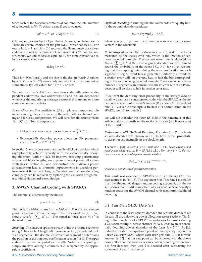
Though all three decoders theoretically have section error-rate decaying to zero with increasing block length for any fixed R < C, the soft-decision decoders have much better empirical perfor-mance [19, 22]. In the following, we illustrate the performance of the AMP decoder for block lengths of the order of a few thou-sands. All the simulation results are obtained using Hadamard-based designs.

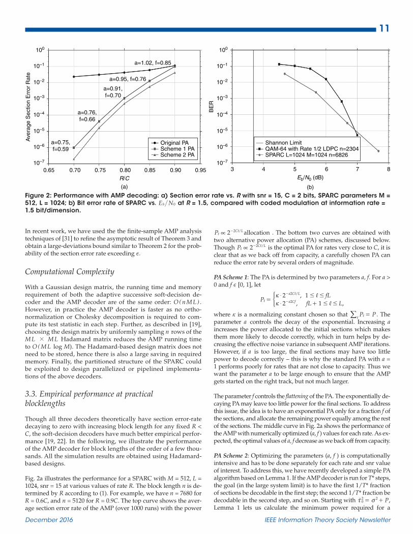
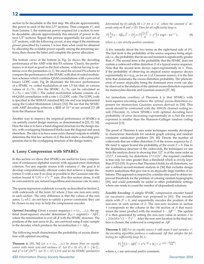
Fig. 2a illustrates the performance for a SPARC with M = 512, L = 1024, snr = 15 at various values of rate R. The block length n is de-termined by R according to (1). For example, we have n = 7680 for R = 0.6C, and n = 5120 for R = 0.9C. The top curve shows the aver-age section error rate of the AMP (over 1000 runs) with the power

P 2 /C L2?, ,- allocation . The bottom two curves are obtained with two alternative power allocation (PA) schemes, discussed below. Though P 2 /C L2?, ,- is the optimal PA for rates very close to C, it is clear that as we back off from capacity, a carefully chosen PA can reduce the error rate by several orders of magnitude.

PA Scheme 1: The PA is determined by two parameters a, f. For a > 0 and f e [0, 1], let

,

, ,P

fLfL L

22

11

/a C L

a Cf

2

2$$

,

,

# ## #

l

l=

+,

,-

-)

where l is a normalizing constant chosen so that P P=,,/ . The

parameter a controls the decay of the exponential. Increasing a increases the power allocated to the initial sections which makes them more likely to decode correctly, which in turn helps by de-creasing the effective noise variance in subsequent AMP iterations. However, if a is too large, the final sections may have too little power to decode correctly – this is why the standard PA with a = 1 performs poorly for rates that are not close to capacity. Thus we want the parameter a to be large enough to ensure that the AMP gets started on the right track, but not much larger.

The parameter f controls the flattening of the PA. The exponentially de-caying PA may leave too little power for the final sections. To address this issue, the idea is to have an exponential PA only for a fraction f of the sections, and allocate the remaining power equally among the rest of the sections. The middle curve in Fig. 2a shows the performance of the AMP with numerically optimized (a, f ) values for each rate. As ex-pected, the optimal values of a, f decrease as we back off from capacity.

PA Scheme 2: Optimizing the parameters (a, f ) is computationally intensive and has to be done separately for each rate and snr value of interest. To address this, we have recently developed a simple PA algorithm based on Lemma 1. If the AMP decoder is run for T* steps, the goal (in the large system limit) is to have the first 1/T* fraction of sections be decodable in the first step; the second 1/T* fraction be decodable in the second step, and so on. Starting with P0

2 2x v= +r , Lemma 1 lets us calculate the minimum power required for a

Figure 2: Performance with AMP decoding: a) Section error rate vs. R with snr = 15, C = 2 bits, SPARC parameters M = 512, L = 1024; b) Bit error rate of SPARC vs. E Nb 0 at R = 1.5, compared with coded modulation at information rate = 1.5 bit/dimension.

100

10–1

10–2

10–3

10–4

10–5

10–6

10–7

100

10–1

10–2

10–3

10–4

10–5

10–6

10–7

0.65

a=0.75,f=0.59

a=0.76,f=0.66

a=0.91,f=0.70

a=0.95, f=0.76

a=1.02, f=0.85

Ave

rage

Sec

tion

Err

or R

ate

BE

R

0.70 0.75 0.80R/C

0.85

(a) (b)

0.90 0.95 3 4 5 6Eb/N0 (dB)

7 8

Original PAScheme 1 PAScheme 2 PA

Shannon LimitQAM-64 with Rate 1/2 LDPC n=2304SPARC L=1024 M=1024 n=6826

12

IEEE Information Theory Society Newsletter December 2016

section to be decodable in the first step. We allocate approximately this power to each of the first L/T* sections. Then compute 1

2xr , and from Lemma 1, the minimum power required for a section to now be decodable; allocate approximately this amount of power to the next L/T* sections. Repeat this process sequentially for each set of L/T* sections, with the following caveat: at any stage if the minimum power prescribed by Lemma 1 is less than what could be obtained by allocating the available power equally among the remaining sec-tions, then choose the latter and complete the power allocation.

The bottom curve at the bottom in Fig. 2a shows the decoding performance of the AMP with this PA scheme. Clearly, the perfor-mance is at least as good as the first scheme, without having to op-timize over the parameters (a, f ). We used the second PA scheme to compare the performance of the SPARC with that of coded modula-tion schemes which combine QAM constellations with a powerful binary LDPC code. Fig 2b illustrates the bit-error performance of a SPARC vs. coded modulation at rate 1.5 bit/dim. at various values of /E Nb 0 . (For the SPARC, E Nb 0 can be calculated as

/ / .E N R2snrb 0 = ^ h h The coded modulation scheme consists of a 64-QAM constellation with a rate 1/2 LDPC code. The LDPC code is specified in the WiMAX standard 802.16e and was implemented using the Coded Modulation Library [32]. We see that the SPARC with AMP decoding achieves a BER of 10−4 at snr around 2.5 dB from the Shannon limit.

Another way to improve the empirical performance of SPARCs is via spatially coupled design matrices, as demonstrated in [23, 33, 34]. Here the idea is to have a band-diagonal structure for the design ma-trix, with overlapping Hadamard blocks near the diagonal and zeros elsewhere. The idea is to have some extra channel outputs to reliably determine the first few sections of b; this kick-starts a decoding pro-gression due to the overlapping structure of the design matrix.

4. Lossy Compression with SPARCs

In this section we show that SPARCs are useful for lossy compres-sion of continuous alphabet sources with squared-error distortion criterion. For any ergodic source with variance v2, the goal is to develop computationally efficient codes that achieve a target dis-tortion D with a rate R as close as possible to the Gaussian rate-dis-tortion bound *R D e R2 2o= -^ h nats. (For this section alone, it will be convenient to use natural logarithms and measure rate in nats.)

The sparse regression codebook is exactly as described in Section 2, with codewords of the form Ab where b has one non-zero entry in each section. The only difference is that the values of the non zeros, nP," ,, do not have to satisfy a power constraint; they can be chosen in any way to help the compression encoder.

Optimal Encoding: Given a source sequence s := (s1,...,sn), the op-timal (least-squares) encoder determines : argmin s Aopt

2b b= -t t ,

where the minimization is over all bt with the SPARC structure. The positions of the non-zeros in optbt are conveyed using R nats/sample to the decoder, which produces the reconstruction s A optb=t t .

The following result characterizes the probability of excess distor-tion with optimal encoding.

Theorem 4. [35, 36] Let : , ,s s sn1 f= ^ h be drawn from an ergodic source with mean zero and variance v2. Let D e (0, v2), lnR D2

1 2

2 v , and ,De R2 2 2! vc ^ h. Let P P L 6,=, ^ h and let the SPARC parameters

determined by (1) satisfy M = La for a a*2 , where the constant a* de-pends only on R and c 2/D. Then for all sufficiently large n,

,expn

s A Dns

n1P Poptc2

22 12 2#b lc- + - +tc c ^m m h (9)

where l, c are strictly positive constants.

A few remarks about the two terms on the right-hand side of (9). The first term is the probability of the source sequence being atypi-cal, i.e., the probability that its second moment is significantly greater than v2. The second term is the probability that the SPARC does not contain a codeword within distortion D of a typical source sequence. Note that the second term decays super-exponentially in n. Thus, if the probability of observing an atypical source sequence decays exponentially in n (e.g., as for an i.i.d. Gaussian source), it is the first term that dominates the excess distortion probability. The phenom-enon of source atypicality being the dominant error event can also be observed in the analysis of the optimal excess-distortion exponent for memoryless discrete and Gaussian sources [37, 38].

An immediate corollary of Theorem 4 is that SPARCs with least-squares encoding achieve the optimal excess-distortion ex-ponent for memoryless Gaussian sources derived in [38]. This result should be contrasted with the AWGN channel coding re-sult (Theorem 1), where SPARCs with optimal decoding have probability of error decreasing exponentially in n, but the error exponent is smaller than the Shannon-Gallager random coding exponent [13].

The proof of Theorem 4 uses some techniques recently developed to characterize thresholds for random graph coloring and random constraint satisfaction problems [39, 40]. Denote the number of codewords that are within distortion D of the source sequence by Z. We need to upper bound the probability of the event Z = 0. Due to the dependence structure of the codewords, the techniques we use boils the analysis down to showing that ZE 2 is of the same order as

ZE 2^ h . Curiously, for distortions .D 0 2 2L o , the required condition is true only for rates greater than a threshold which is strictly larger than R*(D) [35]. To prove that Theorem 4 holds for all distortions, we use a refined second-moment analysis in [36] that excludes design matrix realizations that give rise to an atypically large number of so-lutions. This approach is inspired by a similar idea used to obtain im-proved thresholds for the problem of coloring random hypergraphs [39], and could potentially be useful in other probabilistic settings where one needs to count the number of (dependent) solutions.

Feasible Encoding: A simple SPARC compression encoder based on successive cancellation was proposed in [41]. The encoder starts with b0 = 0, and sequentially encodes the position of the non-zero in each section of b. The non-zero location in section , corresponds to the column in the , th section of A that maxi-mizes the inner product with the residual S A 1b- ,- . The update bl is then generated by setting the non-zero value in section , to

ln M2 1 LR2 2 1o - ,-^ ^h h . After the non-zero location in the final sec-

tion is chosen, the codeword is computed as A Lb .

Theorem 5. [4I] For an ergodic source S with mean 0 and variance o2, the encoding algorithm produces a codeword Abt that satisfies the fol-lowing for sufficiently large M, L:

n S A e e1P lnln ln

MR n c M2 2 22 1b o D- + l D- - -t` cj m

where l, c are universal positive constants.

13

December 2016 IEEE Information Theory Society Newsletter

We can view the encoder as successively refining the source over over ( )lognL n+ stages, with each stage being a rate-distortion code of rate R/L. The first stage is an optimal code of rate R/L for an i.i.d. ,0N 2o^ h source. This implies that the residual r s A1

1b= - satisfies /r n e 1/R L

LR

12 2 2 2 2. .o o -- ^ h. The residual r1 acts as the

‘source’ sequence for the second stage, which is an optimal rate-dis-tortion code for source variance e /R L2 2o - . At the end of the second stage, we have the residual r2, which gets refined by the third stage, and so on. Each stage of refinement reduces the variance of the in-coming residual by a factor of approximately 1 R

L2-^ h. Therefore,

we expect that the final distortion /r n e1 LLR L R2 2 2 2 2. #o o- -^ h .

However, since the rate R/L is infinitesimal, the deviations from the expected distortion in each stage can be significant. The essence of the proof of Theorem 5 is in analyzing these deviations, and showing that the final distortion /r nL

2 is close to the typical value e R2 2o - . We note that such a “hard-decision” successive cancellation approach does not work well for AWGN channel decoding, i.e., the section er-ror rate would decay much slower than exponentially with block length n. One explanation for this is that in channel coding, there is a unique codeword that the decoder has to determine, whereas in lossy compression, the number of good codewords is exponential in n when the rate is larger than the rate-distortion function.

With a Gaussian design matrix, the running time and memory re-quired for the successive cancellation encoder are O(nML). As in chan-nel coding, implementing the compressor with a Hadamard-based design matrix can lead to significant speedup and memory savings.

5. Multi-terminal Source and Channel Coding with SPARCs

Coding schemes that achieve the optimal rate-regions for several multi-terminal source and channel coding models often use the following ingredients: i) rate-optimal point-to-point source and channel codes, and ii) combining or splitting these point-to-point codes via superposition or binning [17].

Superposition with SPARCs: Superposition is easy to implement with SPARCs since the structure of the code itself is motivated by the idea of superposition! Indeed, to construct a superposition codebook with rates R1 and R2, use two design matrices A1, A2 with rates R1, R2, each with block length n. Then the concatenated SPARC defined by the matrix : ,A A A1 2= 6 @ defines a superposi-tion codebook with sum-rate R1 + R2. The message vector b is [b1, b2]T, with b1 and b2 being the messages corresponding to the rate R1 and rate R2 SPARCs, respectively.

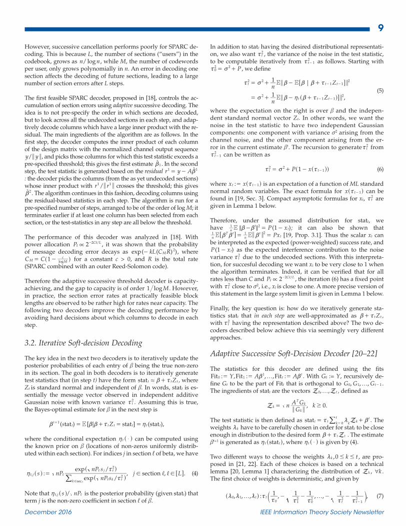
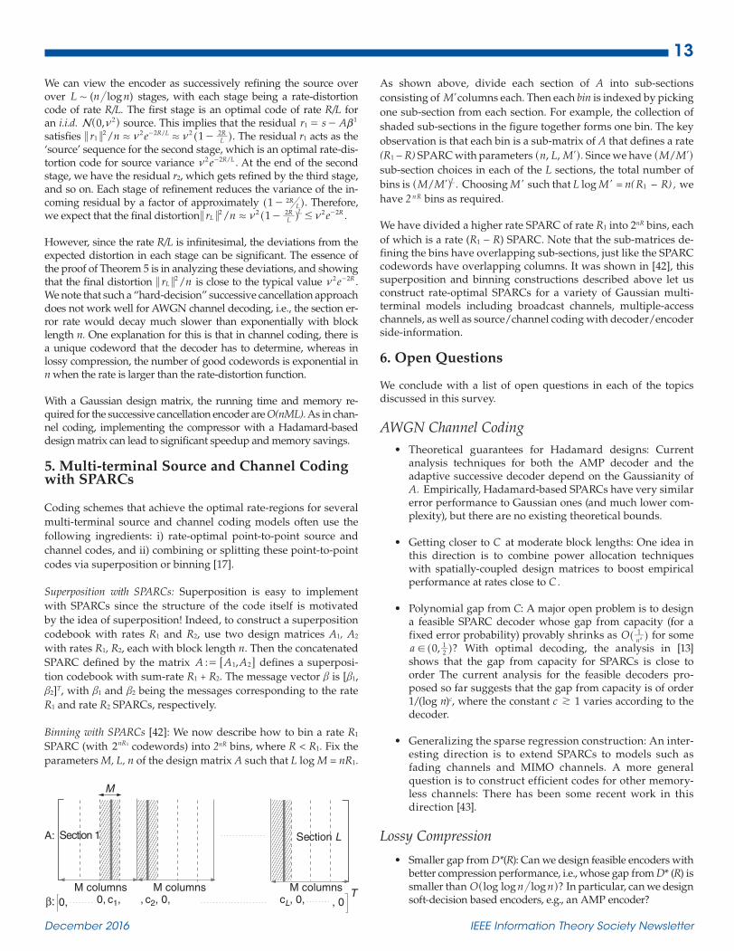
Binning with SPARCs [42]: We now describe how to bin a rate R1

SPARC (with 2nR1 codewords) into 2nR bins, where R < R1. Fix the parameters M, L, n of the design matrix A such that L log M = nR1.

A:

β:T0, c1, cL, 0, , 00,

Section L

M columns M columns M columns

Section 1

, c2, 0,

M �

As shown above, divide each section of A into sub-sections consisting of Mlcolumns each. Then each bin is indexed by picking one sub-section from each section. For example, the collection of shaded sub-sections in the figure together forms one bin. The key observation is that each bin is a sub-matrix of A that defines a rate (R1 − R) SPARC with parameters , ,n L Ml^ h. Since we have /M Ml^ h sub-section choices in each of the L sections, the total number of bins is /M M Ll^ h . Choosing M' such that L log M' = n(R1 − R) , we have 2 nR bins as required.

We have divided a higher rate SPARC of rate R1 into 2nR bins, each of which is a rate (R1 − R) SPARC. Note that the sub-matrices de-fining the bins have overlapping sub-sections, just like the SPARC codewords have overlapping columns. It was shown in [42], this superposition and binning constructions described above let us construct rate-optimal SPARCs for a variety of Gaussian multi-terminal models including broadcast channels, multiple-access channels, as well as source/channel coding with decoder/encoder side-information.

6. Open Questions

We conclude with a list of open questions in each of the topics discussed in this survey.

AWGN Channel CodingTheoretical guarantees for Hadamard designs: Current analysis techniques for both the AMP decoder and the adaptive successive decoder depend on the Gaussianity of A. Empirically, Hadamard-based SPARCs have very similar error performance to Gaussian ones (and much lower com-plexity), but there are no existing theoretical bounds.

Getting closer to C at moderate block lengths: One idea in this direction is to combine power allocation techniques with spatially-coupled design matrices to boost empirical performance at rates close to C .

Polynomial gap from C: A major open problem is to design a feasible SPARC decoder whose gap from capacity (for a fixed error probability) provably shrinks as O n

1a^ h for some

, ?a 0 21! ^ h With optimal decoding, the analysis in [13]

shows that the gap from capacity for SPARCs is close to order The current analysis for the feasible decoders pro-posed so far suggests that the gap from capacity is of order 1/(log n)c, where the constant c L 1 varies according to the decoder.

Generalizing the sparse regression construction: An inter-esting direction is to extend SPARCs to models such as fading channels and MIMO channels. A more general question is to construct efficient codes for other memory-less channels: There has been some recent work in this direction [43].

Lossy Compression

Smaller gap from D*(R): Can we design feasible encoders with better compression performance, i.e., whose gap from D* (R) is smaller than ?log log logO n n^ h In particular, can we design soft-decision based encoders, e.g., an AMP encoder?

14

IEEE Information Theory Society Newsletter December 2016

Bernoulli dictionaries: Can one extend the results for optimal encoding and successive cancellation encoding (which are proved for Gaussian dictionaries) to dictionar-ies with i.i.d. !1 entries? For AWGN channels, SPARC ML decoding with i.i.d. !1 design matrices has been analyzed in [14].

Finite-alphabet lossy compression: Can one use SPARC-like constructions to compress to finite alphabet sources, e.g., binary sources with Hamming distortion?

Multi-terminal models

Approaching the Shannon limits with feasible encoding and decoding: The construction in Sec. 5 implements bin-ning by nesting a lower-rate source/channel code inside a higher-rate channel/source code. Since the optimal power allocation for feasible encoding/decoding will depend on the rate, we may not be able to ensure that the SPARC power allocation is simultaneously optimal for both the high-rate and low-rate codes.

An open question is: how to do we design good PA schemes for problems that require binning so that both the high-rate and low-rate codes are close to their Shannon limits, thereby ensuring that the overall rate is also near-optimal? We note that PA is not an issue when we use optimal encoding and decoding, as flat power-allocation is sufficient at all rates.

Implementing SPARCs at near-optimal rates for basic mod-els with binning (such as Gaussian Wyner-Ziv and ‘writing on dirty paper’) will pave the way to construct low-com-plexity, rate-optimal codes for a variety of Gaussian multi-terminal models such as multiple descriptions, distributed lossy compression, and relay channels.

Acknowledgements

This survey is based on work done in collaboration with Sang-hee Cho, Adam Greig, Antony Joseph, Cynthia Rush, and Tuhin Sarkar. The work was supported in part by the National Science Foundation under Grant CCF-1217023, and by a Marie Curie Career Integration Grant (GA No. 631489) from the European Commission.

References

[1] C. Berrou and A. Glavieux, “Near optimum error correcting coding and decoding: turbo-codes,” IEEE Transactions on Commu-nications, vol. 44, pp. 1261–1271, Oct 1996.

[2] T. Richardson and R. Urbanke, Modern Coding Theory. Cam-bridge University Press, 2008.

[3] E. Arikan, “Channel polarization: A method for constructing capacity-achieving codes for symmetric binary-input memoryless channels,” IEEE Trans. Inf. Theory, vol. 55, pp. 3051–3073, July 2009.

[4] S. Korada and R. Urbanke, “Polar codes are optimal for lossy source coding,” IEEE Trans. Inf. Theory, vol. 56, pp. 1751–1768, April 2010.

[5] S. Kudekar, T. Richardson, and R. L. Urbanke, “Spatially cou-pled ensembles universally achieve capacity under belief propaga-tion,” IEEE Trans. Inf. Theory, vol. 59, pp. 7761–7813, December 2013.

[6] G. D. Forney and G. Ungerboeck, “Modulation and coding for linear gaussian channels,” IEEE Transactions on Information Theory, vol. 44, no. 6, pp. 2384–2415, 1998.

[7] A. Guillén i Fàbregas, A. Martinez, and G. Caire, Bit-interleaved coded modulation. Now Publishers Inc, 2008.

[8] G. Böcherer, F. Steiner, and P. Schulte, “Bandwidth efficient and rate-matched low-density parity-check coded modulation,” IEEE Transactions on Communications, vol. 63, no. 12, pp. 4651–4665, 2015.

[9] R. Zamir, Lattice Coding for Signals and Networks: A Structured Coding Approach to Quantization, Modulation, and Multiuser Informa-tion Theory. Cambridge University Press, 2014.

[10] U. Erez and R. Zamir, “Achieving 1/2 log(1 + snr) on the AWGN channel with lattice encoding and decoding,” IEEE Trans. Inf. Theory, vol. 50, no. 10, pp. 2293–2314, 2004.

[11] N. Sommer, M. Feder, and O. Shalvi, “Low-density lattice codes,” IEEE Trans. Inf. Theory, vol. 54, no. 4, pp. 1561–1585, 2008.

[12] Y. Yan, L. Liu, C. Ling, and X. Wu, “Construction of capac-ity-achieving lattice codes: Polar lattices,” arXiv preprint arX-iv:1411.0187, 2014.

[13] A. Barron and A. Joseph, “Least squares superposition codes of moderate dictionary size are reliable at rates up to capacity,” IEEE Trans. on Inf. Theory, vol. 58, pp. 2541–2557, Feb. 2012.

[14] Y. Takeishi, M. Kawakita, and J. Takeuchi, “Least squares superposition codes with Bernoulli dictionary are still reliable at rates up to capacity,” IEEE Trans. Inf. Theory, vol. 60, pp. 2737–2750, May 2014.

[15] Y. Takeishi and J. Takeuchi, “An improved upper bound on block error probability of least squares superposition codes with unbiased bernoulli dictionary,” in Proc. IEEE Int. Symp. Inf. Theory, pp. 1168–1172, 2016.

[16] T. M. Cover and J. A. Thomas, Elements of Information Theory. John Wiley and Sons, 2012.

[17] A. El Gamal and Y.-H. Kim, Network Information Theory. Cam-bridge University Press, 2011.

[18] A. Joseph and A. R. Barron, “Fast sparse superposition codes have near exponential error probability for R < C,”IEEE Trans. Inf. Theory, vol. 60, pp. 919–942, Feb. 2014.

[19] C. Rush, A. Greig, and R. Venkataramanan, “Capacity-achieving sparse superposition codes via approximate message passing decod-ing,” arXiv:1501.05892, 2015. (Shorter version appeared in ISIT ’15).

[20] A. R. Barron and S. Cho, “High-rate sparse superposition codes with iteratively optimal estimates,” in Proc. IEEE Int. Symp. Inf. Theory, 2012.

15

December 2016 IEEE Information Theory Society Newsletter

[21] S. Cho and A. Barron, “Approximate iterative bayes optimal estimates for high-rate sparse superposition codes,” in Sixth Work-shop on Information-Theoretic Methods in Science and Engineering, 2013.

[22] S. Cho, High-dimensional regression with random design, includ-ing sparse superposition codes. PhD thesis, Yale University, 2014.

[23] J. Barbier and F. Krzakala, “Approximate message-passing decoder and capacity-achieving sparse superposition codes,” arXiv:1503.08040, 2015.

[24] D. L. Donoho, A. Maleki, and A. Montanari, “Message-pass-ing algorithms for compressed sensing,” Proceedings of the National Academy of Sciences, vol. 106, no. 45, pp. 18914–18919, 2009.

[25] A. Montanari, “Graphical models concepts in compressed sensing,” in Compressed Sensing (Y. C. Eldar and G. Kutyniok, eds.), pp. 394–438, Cambridge University Press, 2012.

[26] M. Bayati and A. Montanari, “The dynamics of message pass-ing on dense graphs, with applications to compressed sensing,” IEEE Trans. Inf. Theory, pp. 764–785, 2011.

[27] M. Bayati and A. Montanari, “The LASSO risk for Gaussian matrices,” IEEE Trans. Inf. Theory, vol. 58, no. 4, pp. 1997–2017, 2012.

[28] F. Krzakala, M. Mézard, F. Sausset, Y. Sun, and L. Zdeborová, “Probabilistic reconstruction in compressed sensing: algorithms, phase diagrams, and threshold achieving matrices,” Journal of Sta-tistical Mechanics: Theory and Experiment, no. 8, 2012.

[29] S. Rangan, “Generalized approximate message passing for es-timation with random linear mixing,” in Proc. IEEE Int. Symp. Inf. Theory, pp. 2168–2172, 2011.

[30] D. L. Donoho, A. Javanmard, and A. Montanari, “Informa-tion-theoretically optimal compressed sensing via spatial cou-pling and approximate message passing,” IEEE Trans. Inf. Theory, pp. 7434–7464, Nov. 2013.

[31] C. Rush and R. Venkataramanan, “Finite sample analysis of approximate message passing,” in Proc. IEEE Int. Symp. Inf. Theory, 2016. Full version: https://arxiv.org/abs/1606.01800.

[32] “Coded modualtion library.” Online: http://www.iteratives-olutions.com/Matlab.htm.

[33] J. Barbier, C. Schülke, and F. Krzakala, “Approximate mes-sage-passing with spatially coupled structured operators, with applications to compressed sensing and sparse superposition codes,” Journal of Statistical Mechanics: Theory and Experiment, no. 5, 2015.

[34] J. Barbier, M. Dia, and N. Macris, “Proof of threshold satu-ration for spatially coupled sparse superposition codes,” in Proc. IEEE Int. Symp. Inf. Theory, 2016.

[35] R. Venkataramanan, A. Joseph, and S. Tatikonda, “Lossy compression via sparse linear regression: Performance under minimum-distance encoding,” IEEE Trans. Inf. Thy, vol. 60, pp. 3254–3264, June 2014.

[36] R. Venkataramanan and S. Tatikonda, “The rate-distortion function and error exponent of sparse regression codes with op-timal encoding,” arXiv:1401.5272, 2014. (Shorter version appeared in ISIT ’14).

[37] K. Marton, “Error exponent for source coding with a fi-delity criterion,” IEEE Trans. Inf. Theory, vol. 20, pp. 197–199, Mar 1974.

[38] S. Ihara and M. Kubo, “Error exponent for coding of memory-less Gaussian sources with a fidelity criterion,” IEICE Trans. Fun-damentals, vol. E83-A, pp. 1891–1897, Oct. 2000.

[39] A. Coja-Oghlan and L. Zdeborová, “The condensation transi-tion in random hypergraph 2-coloring,” in Proc. 23rd Annual ACM-SIAM Symp. on Discrete Algorithms (SODA), pp. 241–250, 2012.

[40] A. Coja-Oghlan and D. Vilenchik, “Chasing the k-colorability threshold,” in Proc. IEEE 54th Annual Symposium on Foundations of Computer Science (FOCS), pp. 380–389, 2013.

[41] R. Venkataramanan, T. Sarkar, and S. Tatikonda, “Lossy com-pression via sparse linear regression: Computationally efficient encoding and decoding,” IEEE Trans. Inf. Theory, vol. 60, pp. 3265–3278, June 2014.

[42] R. Venkataramanan and S. Tatikonda, “Sparse regression codes for multi-terminal source and channel coding,” in 50th Al-lerton Conf. on Commun., Control, and Computing, 2012.

[43] J. Barbier, M. Dia, and N. Macris, “Threshold saturation of spatially coupled sparse superposition codes for all memoryless channels,” in Proc. Inf. Theory Workshop, 2016.