spate: an R Package for Statistical Modeling with

SPDE Based Spatio-Temporal Gaussian Processes

Fabio Sigrist, Hans R. Kunsch, Werner A. Stahel

Seminar for Statistics, Department of Mathematics, ETH Zurich

8092 Zurich, Switzerland

January 22, 2015

Abstract

The R package spate provides tools for modeling of large space-timedata sets. A spatio-temporal Gaussian process is defined through a stochas-tic partial differential equation (SPDE) which is solved using spectralmethods. In contrast to the traditional Geostatistical way of relying onthe covariance function, the spectral SPDE approach is computationallytractable and provides a realistic space-time parametrization.

This package aims at providing tools for two different modeling ap-proaches. First, the SPDE based spatio-temporal model can be used asa component in a customized hierarchical Bayesian model (HBM) or gen-erlized linear mixed model (GLMM). The functions of the package thenprovide parametrizations of the process part of the model as well as com-putationally efficient algorithms needed for doing inference with the hierar-chical model. Alternatively, the adaptive MCMC algorithm implementedin the package can be used as an algorithm for doing inference withoutany additional modeling. The MCMC algorithm supports data that fol-low a Gaussian or a censored distribution with point mass at zero. Spatio-temporal covariates can be included in the model through a regressionterm.

1

Contents

1 Introduction 3

1.1 Notation . . . . . . . . . . . . . . . . . . . . . . . . . . . . . . . . 3

2 Summary of modeling background 4

2.1 Space-time Gaussian process defined through an SPDE . . . . . . 42.2 Spectral solution . . . . . . . . . . . . . . . . . . . . . . . . . . . 52.3 Non-Gaussian data, covariates, and missing data . . . . . . . . . 72.4 Computationally efficient frequentist and Bayesian inference . . . 82.5 Dimension reduction . . . . . . . . . . . . . . . . . . . . . . . . . 8

3 Parametrization of the dynamic space-time model 9

3.1 Innovation spectrum Q and Matern spectrum . . . . . . . . . . . 93.2 Propagator matrix G . . . . . . . . . . . . . . . . . . . . . . . . . 93.3 Two-dimensional real Fourier transform . . . . . . . . . . . . . . 11

4 Simulation and plotting 13

5 Inference: log-likelihood evaluation and sampling from the full

conditional 14

5.1 Example of use of sample.four.coef . . . . . . . . . . . . . . . 145.2 Example of use of loglike . . . . . . . . . . . . . . . . . . . . . 155.3 Maximum likelihood estimation . . . . . . . . . . . . . . . . . . . 165.4 Bayesian inference using MCMC . . . . . . . . . . . . . . . . . . 17

5.4.1 Skewed Tobit model and missing data . . . . . . . . . . . 18

6 An MCMC algorithm 18

6.1 Arguments of spate.mcmc . . . . . . . . . . . . . . . . . . . . . . 196.2 Additional fine tuning . . . . . . . . . . . . . . . . . . . . . . . . 196.3 An example of the use of spate.mcmc . . . . . . . . . . . . . . . 206.4 Making predictions with spate.predict . . . . . . . . . . . . . . 22

2

1 Introduction

Increasingly larger spatio-temporal data arise in many fields and applications.For instance, data sets are obtained from remote sensing satellites or deter-ministic physical models such as numerical weather prediction (NWP) models.Hence, there is a growing need for methodology that can cope with such largedata. See Cressie and Wikle (2011) for an introduction and an overview ofspatio-temporal statistics.

Gaussian processes are often used for modeling data in space and time. AGaussian process is defined by specifying a mean and a covariance function.However, directly working with a spatio-temporal covariance function is com-putationally infeasible if data sets are large. This is due to the fact that fordoing inference, frequentist or Bayesian, covariance matrices need to be factor-ized which is computationally expensive. Alternatively, a Gaussian process canbe specified through a stochastic partial differential equation (SPDE), whichimplicitly also gives a covariance function. The advection-diffusion SPDE is anelementary model in the spatio-temporal setting. When solving this SPDE inthe spectral space, and discretizing in time and space, a linear Gaussian statespace model is obtained which is computationally advantageous (see Sigrist et al.(2012)). Roughly speaking, the computational speed-up is due to the tempo-ral Markov property and the fact that Fourier functions are eigenfunctions ofthe differential operator, from which follows that in the spectral space most ofthe relevant matrices are diagonal. This package implements the methodologypresented in Sigrist et al. (2012).

The package spate has the following functionality. On the one hand, itprovides tools for constructing customized models such as generalized linearmixed models (GLMM) or hierarchical Bayesian models (HBM) (Wikle et al.,1998) using a spatio-temporal Gaussian process at some stage, for instance, inthe linear predictor. These tools include functions for obtaining spectral prop-agator and covariance matrices of the linear Gaussian state space model, fastcalculation of the two-dimensional real Fourier transform, reduced dimensionalapproximations, fast evaluation of the log-likelihood, and fast simulation fromthe full conditional of the Fourier coefficients using a spectral variant of theForward Filtering Backward Sampling algorithm. On the other hand, the pack-age also provides a function for Bayesian inference using a Monte Carlo Markovchain (MCMC) algorithm that is designed such that it needs as little fine tuningas possible. The MCMC algorithm can model data being normally distributedor censored data with point mass at zero following a skewed Tobit distribution.There is also a function for making probabilistic predictions. A user interestedin modeling data not following one of the above two types of data distributionscan modify the MCMC algorithm to allow for different distributions. Finally,functions for plotting and simulation of space-time processes are also provided.

1.1 Notation

Since some readers might skip the next section, we start by establishing theprincipal notation. The Gaussian process modeling structured variation in space

3

and time is denoted by ξ(ti, sl), i = 1, . . . , T , l = 1, . . . , N . In vectorized form,we write ξ(ti) = (ξ(ti, s1), . . . , ξ(ti, sN ))′ (where stacking is done first over thex-axis and then over the y-axis), and ξ = (ξ(t1)

′, . . . , ξ(tT )′)′. For each ti,

ξ(ti) = Φα(ti) is the Fourier transform of the Fourier coefficients α(ti), α =(α(t1)

′, . . . ,α(tT )′)′. The observed Gaussian process w(ti, sl) equals the latent

ξ(ti, sl) plus a measurement error. w(ti) and w are defined analogously. If theobservations are censored, i.e., if they follow a skewed Tobit distribution, theobserved data is denoted by y(ti, sl). Finally, θ = (ρ0, σ

2, ζ, ρ1, γ, α, µx, µy, τ2)′

denotes the vector of hyper-parameters.We assume that we model the process on a regular, rectangular grid of

n× n = N spatial locations s1, . . . , sN in [0, 1]2 and at equidistant time pointst1, . . . , tT with ti − ti−1 = ∆. These two assumptions can be easily relaxed,i.e., one can have irregular spatial locations and non-equidistant time points.The former can be achieved by adopting a data augmentation approach (im-plemented in spate.mcmc) or by using an incidence matrix (also implementedin spate.mcmc, see below) depending on the dimensionality of the observationprocess. The latter can be done by taking a time varying ∆i.

2 Summary of modeling background

In the following, we briefly recall the underlying model and methodology. Formore details we refer to Sigrist et al. (2012).

2.1 Space-time Gaussian process defined through an SPDE

A spatio-temporal Gaussian process ξ(t, s) is defined as the solution of thestochastic advection-diffusion equation

∂

∂tξ(t, s) = −µ · ∇ξ(t, s) +∇ ·Σ∇ξ(t, s)− ζξ(t, s) + ǫ(t, s), (1)

where t ≥ 0, s ∈ [0, 1]2 wrapped on a torus, ∇ =(

∂∂x ,

∂∂y

)′

is the gradient

operator, and ∇ · F = ∂Fx

∂x + ∂F y

∂y is the divergence operator for F = (F x, F y)′

being a vector field, µ = (µx, µy)′,

Σ−1 =1

ρ21

(cosα sinα

−γ · sinα γ · cosα

)T (cosα sinα

−γ · sinα γ · cosα

),

and where ǫ(t, s) is a Gaussian random field that is white in time and has aspatial Matern covariance function with spectral density

f(k) =σ2

(2π)2

(kk +

1

ρ20

)−(ν+1)

.

For the parameters, we have the following restrictions

ρ0, σ, ρ1, γ, ζ ≥ 0, µx, µy ∈ [−0.5, 0.5], α ∈ [0, π/2].

4

The parameters are interpreted as follows. The first term µ · ∇ξ(t, s) modelstransport effects (called advection in weather applications), µ being a driftor velocity vector. The second term, ∇ · Σ∇ξ(t, s), is a diffusion term thatcan incorporate anisotropy. ρ1 acts as a range parameter and controls theamount of diffusion. The parameters γ and α control the amount and thedirection of anisotropy. With γ = 1, isotropic diffusion is obtained. Removinga certain amount of ξ(t, s) at each time, −ζξ(t, s) accounts for damping andregulates the amount of temporal correlation. Finally, ǫ(t, s) is a source-sink orstochastic forcing term that can be interpreted as describing, amongst others,convective phenomena in precipitation modeling applications. ρ0 is a rangeparameter and σ2 determines the marginal variance. Since in many applicationsthe smoothness parameter ν is not estimable from data, we take ν = 1 bydefault, which corresponds to the Whittle covariance function.

2.2 Spectral solution

As is shown in Sigrist et al. (2012), inference can be done computationally effi-ciently when solving the SPDE in the spectral space. The latter means, roughlyspeaking, that the solution is represented a linear combination of deterministic,real Fourier basis functions

φ(c)j (s) = cos(k′

js), φ(s)j (s) = sin(k′

js),

with random coefficients αcj(t), α

sj(t) that evolve dynamically over time accord-

ing to a vector autoregression. Fourier functions have several advantages forsolving the SPDE (1). Amongst others, Fourier functions are eigenfunctionsof the spatial differential operator: differentiation in the physical space corre-sponds to multiplication in the spectral space. Furthermore, one can use theFFT for efficiently transforming from the physical to the spectral space, andvice versa.

As is customary for spatial and spatio-temporal models, we add an non-structured Gaussian term ν(t, s) ∼ N(0, τ2) that is white in time and spaceto ξ(t, s). This term accounts for small scale variation and / or measurementerrors (nugget effect). Solving the SPDE in the spectral space and discretizingin time and space, we obtain the following linear Gaussian state space model:

w(ti+1) = ξ(ti+1) + ν(ti+1),ν(ti+1) ∼ N(0, τ21), (2)

ξ(ti+1) = Φα(ti+1), (3)

α(ti+1) = Gα(ti) + ǫ(ti+1), ǫ(ti+1) ∼ N(0, Q). (4)

The observation equation (2) specifies how the observation field w(ti+1) =(w(ti, s1), . . . , w(ti, sN ))′ at time ti+1 is related to the spatio-temporal processξ(ti+1). See below on how to handle non-Gaussian data. In the second equation(3), the matrix Φ,

Φ =[φ(s1), . . . ,φ(sN )

]′

φ(sl) =(φ(c)1 (sl), . . . , φ

(c)4 (sl), φ

(c)5 (sl), φ

(s)5 (sl), . . . , φ

(c)(K−4)/2(sl), φ

(s)(K−4)/2(sl)

)′

,

5

applies the discrete, real Fourier transformation to the coefficients

α(t) =(α(c)1 (t), . . . , α

(c)4 (t), α

(c)5 (t), α

(s)5 (t), . . . , α

(c)(K−4)/2(t), α

(s)(K−4)/2(t)

)′

.

Note that the first four terms are cosine terms and, afterwards, there are cosine- sine pairs. This is a peculiarity of the real Fourier transform. It is due to thefact that for four wavenumbers kj , the sine terms equal zero on the grid (seeFigure 1). We use the real Fourier transform, instead of the complex one, inorder to avoid complex numbers in the propagator matrix G and since data isusually real. Note that due to the use of Fourier functions, we assume spatialstationarity for both the solution ξ and the innovation term ǫ.

The third equation (4) specifies how the random Fourier coefficients evolvedynamically over time. The propagator matrix G is a block diagonal matrixwith 2×2 blocks, and the innovation covariance matrix Q is a diagonal matrix.These two matrices are defined as follows:

G = e∆H ,

[H]1:4,1:4 = diag(−k′

jΣkj − ζ),

[H]5:K,5:K = diag

(−k′

jΣkj − ζ −µkj

µkj −k′

jΣkj − ζ

),

(5)

and

Q = diag

(f(kj)

1− e−2∆(k′

jΣkj+ζ)

2(k′

jΣkj + ζ)

). (6)

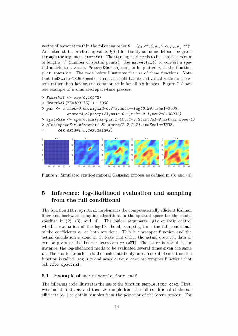
Figure 4 shows an example of a propagator matrix G.The above result is given in vector format. For the sake of understanding,

we can also write that the solution is of the form

ξ(t, sl) =4∑

l=1

α(c)j (t)φ

(c)j (sl)

+

K/2+2∑

l=5

α(c)j (t)φ

(c)j (sl) + α

(s)j (t)φ

(s)j (sl)

=φ(sl)′α(t),

(7)

whereK denotes the number of Fourier terms, i.e., K = N . K however does notnecessary need to equal N , see below for a discussion on dimension reduction.

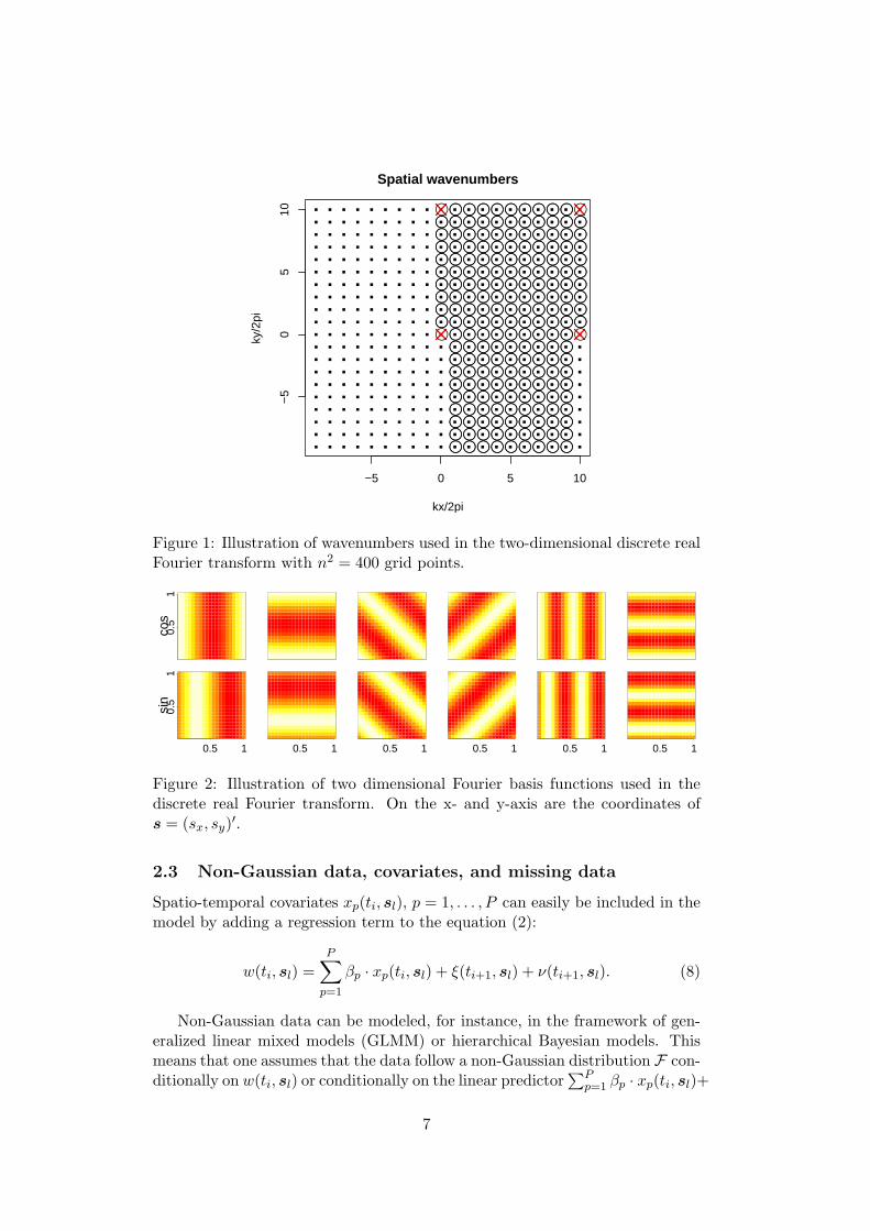
The spatial wavenumbers kj used in the real Fourier transform lie on then × n grid Dn = {2π · (i, j) : −(n/2 + 1) ≤ i, j ≤ n/2} ⊂ 2π · Z2 with n2 =N . Figure 1 illustrates the spatial wavenumbers on a 20 × 20 grid. The redcrosses mark the first four spatial wavenumbers having only a cosine term. Theremaining dots with a circle around represent the wavenumbers used by thecosine - sine pairs in the real Fourier transform.

To get an idea how the basis functions cos (k′

js) and sin (k′

js) look like, weplot in Figure 2 twelve low-frequency basis functions corresponding to the sixspatial frequencies closest to the origin 0 (see Figure 1).

6

Spatial wavenumbers

kx/2pi

ky/2

pi

−5 0 5 10

−5

05

10

● ●

● ●

●● ●● ●● ●● ●● ●● ●● ●● ●●●● ●● ●● ●● ●● ●● ●● ●● ●● ●● ●●●● ●● ●● ●● ●● ●● ●● ●● ●● ●● ●●●● ●● ●● ●● ●● ●● ●● ●● ●● ●● ●●●● ●● ●● ●● ●● ●● ●● ●● ●● ●● ●●●● ●● ●● ●● ●● ●● ●● ●● ●● ●● ●●●● ●● ●● ●● ●● ●● ●● ●● ●● ●● ●●●● ●● ●● ●● ●● ●● ●● ●● ●● ●● ●●●● ●● ●● ●● ●● ●● ●● ●● ●● ●● ●●●● ●● ●● ●● ●● ●● ●● ●● ●● ●● ●●

●● ●● ●● ●● ●● ●● ●● ●● ●●

●● ●● ●● ●● ●● ●● ●● ●● ●●●● ●● ●● ●● ●● ●● ●● ●● ●●●● ●● ●● ●● ●● ●● ●● ●● ●●●● ●● ●● ●● ●● ●● ●● ●● ●●●● ●● ●● ●● ●● ●● ●● ●● ●●●● ●● ●● ●● ●● ●● ●● ●● ●●●● ●● ●● ●● ●● ●● ●● ●● ●●●● ●● ●● ●● ●● ●● ●● ●● ●●●● ●● ●● ●● ●● ●● ●● ●● ●●

Figure 1: Illustration of wavenumbers used in the two-dimensional discrete realFourier transform with n2 = 400 grid points.

cos

0.5

1si

n0.

51

0.5 1 0.5 1 0.5 1 0.5 1 0.5 1 0.5 1

Figure 2: Illustration of two dimensional Fourier basis functions used in thediscrete real Fourier transform. On the x- and y-axis are the coordinates ofs = (sx, sy)

′.

2.3 Non-Gaussian data, covariates, and missing data

Spatio-temporal covariates xp(ti, sl), p = 1, . . . , P can easily be included in themodel by adding a regression term to the equation (2):

w(ti, sl) =

P∑

p=1

βp · xp(ti, sl) + ξ(ti+1, sl) + ν(ti+1, sl). (8)

Non-Gaussian data can be modeled, for instance, in the framework of gen-eralized linear mixed models (GLMM) or hierarchical Bayesian models. Thismeans that one assumes that the data follow a non-Gaussian distribution F con-ditionally on w(ti, sl) or conditionally on the linear predictor

∑Pp=1 βp · xp(ti, sl)+

7

ξ(ti+1, sl). Note that fitting such models is a non-trivial task and subject toongoing research.

Another approach, which avoids adding an additional stochastic level, isto assume that the data is a transformed version of w(ti, sl). For instance, ifthe observations follow a skewed Tobit model, then the we have the followingobservation relation

y(ti, sl) = max(0, w(ti, sl))λ, (9)

where now y(ti, sl) denotes the observed values and w(ti, sl) is a latent Gaussianfield. This data model is implemented in the package spate. Such a model isoften used for modeling precipitation.

Furthermore, missing values, and the censored ones in (9), can be easily dealtwith using a data augmentation approach. See, e.g., Sigrist et al. (2012) formore details. In particular, if the observations do not lie on a regular spatialgrid, the grid cells where no observations are made can be assumed to havemissing data.

2.4 Computationally efficient frequentist and Bayesian infer-

ence

When doing inference, for both data models, the Gaussian one in (2) and thetransformed Tobit model (9), the main difficulty consists in evaluating the like-lihood ℓ(θ) = P [θ|w], θ = (ρ0, σ

2, ζ, ρ1, γ, α, µx, µy, τ2)′, and in simulating from

the full conditional of the coefficients [α|w,θ], where w and α denote the fullspace-time fields. As shown in Sigrist et al. (2012), this can be done in O(TN)time in the spectral space using the Kalman filter and a backward samplingstep. The fast Fourier transform (FFT) can be used to transform between thephysical and the spectral space. Since there are T fields of dimension N (= n2),the costs for this are O(TN logN).

2.5 Dimension reduction

The total computational costs can be additionally alleviated by using a reduceddimensional Fourier basis with K << N basis functions. This means that oneincludes only certain frequencies, e.g., low ones. The spectral filtering andsampling algorithms then require O(KT ) operations. For using the FFT, thefrequencies being excluded are just set to zero.

Alternatively, when the observation process is irregular and low-dimensionalin space, one can include an incidence matrix I that relates the process on thegrid to the observation locations. Instead of (2), the observation equation isthen

w(ti+1) = IΦα(ti+1) + ν(ti+1), ν(ti+1) ∼ N(0, τ21K). (10)

The FFT cannot be used anymore, and the total computational costs areO(K3T ) due to the traditional FFBS.

8

3 Parametrization of the dynamic space-time model

3.1 Innovation spectrum Q and Matern spectrum

The function innov.spec returns the spectrum Q of the integrated stochasticinnovation field ǫ(ti+1) as specified in (6). Similarly, the function matern.spec

returns the spectrum of the Matern covariance function. Note that the Maternspectrum is renormalized, by dividing with the sum over all frequencies so thatthey sum to one. This guarantees that the parameter σ2 is the marginal varianceno matter how many wavenumbers are included, in case dimension reduction isdone and some frequencies are set to zero.

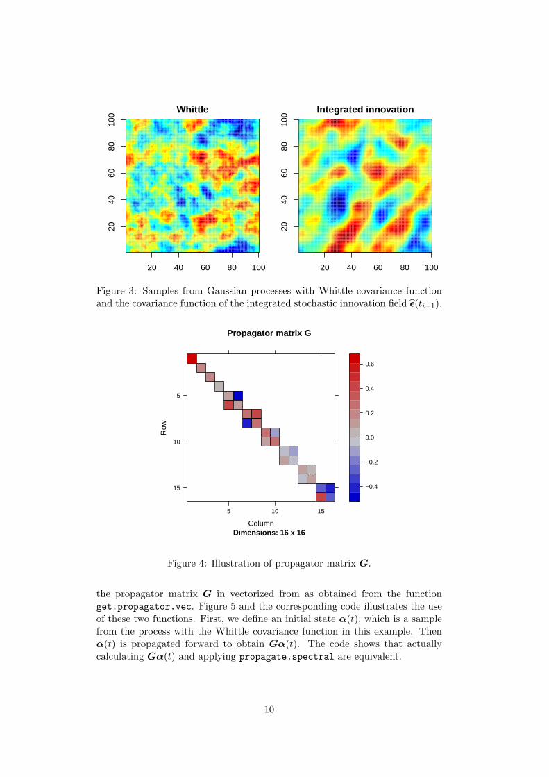
The code below illustrates how these functions are used. First a vector ofindependent Gaussian random variables with variances according to the desiredspectrum is simulated. For instance, ǫ ∼ N(0, Q). In the example, this is donefor the Whittle and the integrated innovation spectrum specified in (6). Thenits Fourier transform Φǫ is calculated to obtain a sample from the spatial fieldwith corresponding spectrum. See two sections below for more details on how tocalculate the Fourier transform. Figure 3 shows sample fields from the Whittleprocess and from the stochastic innovation process.

> n <- 100

> set.seed(1)

> ## Simulate Matern field

> matern.spec <- matern.spec(wave=spate.init(n=n,T=1)[["wave"]],

+ n=n,rho0=0.05,sigma2=1,norm=TRUE)

> matern.sim <- real.fft(sqrt(matern.spec)*rnorm(n*n),n=n,inv=FALSE)

> ## Simulate stochstic innovation field epsilon

> innov.spec <- innov.spec(wave=spate.init(n=n,T=1)[["wave"]],

+ n=n, rho0=0.05, sigma2=1, zeta=0.5,

+ rho1=0.05, alpha=pi/4, gamma=2,norm=TRUE)

> innov.sim <- real.fft(sqrt(innov.spec)*rnorm(n*n),n=n,inv=FALSE)

3.2 Propagator matrix G

The function get.propagator returns the spectral propagator matrix G asdefined in (5). Figure 4 shows an example of a propagator matrix G. The codebefore the figure illustrates how get.propagator is used.

> n <- 4

> wave <- wave.numbers(n)

> G <- get.propagator(wave=wave[["wave"]], indCos=wave[["indCos"]], zeta=0.5,

+ rho1=0.1,gamma=2, alpha=pi/4, muX=0.2, muY=-0.15)

Alternatively, the function propagate.spectral propagates a state α(t)to obtain Gα(t) in a computationally efficient way using the block-diagonalstructure of G. Note that this is a wrapper function of a C function. In general,it is preferable to use propagate.spectral instead of calculating a matrixmultiplication with G. The function propagate.spectral has as argument

9

20 40 60 80 100

2040

6080

100

Whittle

20 40 60 80 100

2040

6080

100

Integrated innovation

Figure 3: Samples from Gaussian processes with Whittle covariance functionand the covariance function of the integrated stochastic innovation field ǫ(ti+1).

Propagator matrix G

Dimensions: 16 x 16Column

Row

5

10

15

5 10 15

−0.4

−0.2

0.0

0.2

0.4

0.6

Figure 4: Illustration of propagator matrix G.

the propagator matrix G in vectorized from as obtained from the functionget.propagator.vec. Figure 5 and the corresponding code illustrates the useof these two functions. First, we define an initial state α(t), which is a samplefrom the process with the Whittle covariance function in this example. Thenα(t) is propagated forward to obtain Gα(t). The code shows that actuallycalculating Gα(t) and applying propagate.spectral are equivalent.

10

> n <- 50

> wave <- wave.numbers(n)

> spec <- matern.spec(wave=wave[["wave"]],n=n,

+ rho0=0.05,sigma2=1,norm=TRUE)

> ## Initial state

> alphat <- sqrt(spec)*rnorm(n*n)

> ## Propagate state

> G <- get.propagator(wave=wave[["wave"]],indCos=wave[["indCos"]],zeta=0.1,

+ rho1=0.02, gamma=2,alpha=pi/4,muX=0.2,muY=0.2,dt=1,ns=4)

> alphat1a <- as.vector(G%*%alphat)

> Gvec <- get.propagator.vec(wave=wave[["wave"]],indCos=wave[["indCos"]],zeta=0.1,

+ rho1=0.02, gamma=2,alpha=pi/4,muX=0.2,muY=0.2,dt=1,ns=4)

> alphat1b <- propagate.spectral(alphat,n=n,Gvec=Gvec)

> ## Both methods do the same thing:

> sum(abs(alphat1a-alphat1b))

[1] 0

10 20 30 40 50

1020

3040

50

Whittle field

10 20 30 40 50

1020

3040

50

Propagated field

Figure 5: Illustration of spectral propagation: initial and propagated field.

3.3 Two-dimensional real Fourier transform

The function real.fft calculates the fast two-dimensional real Fourier trans-form. This is a wrapper function of a C function which uses the complex FFTfunction from the fftw3 library. Furthermore, the function real.fft.TS cal-culates the two-dimensional real Fourier transform of a space-time field for alltime points at once. To be more specific, for each time point, the correspondingspatial field is transformed. In contrast to using T times the function real.FFT,R needs to communicate with C only once which saves considerable computa-tional time, depending on the data size. For an example of the use of real.fft,see two sections above.

11

The function wave.number returns the wavenumbers used in the real Fouriertransform. In contrast to the complex Fourier transform, which uses n2 differentwavenumbers kj on a square grid, the real Fourier transform uses n2/2 + 2different wavenumbers. As mentioned earlier, four of them have only a cosineterm, and the remaining n2/2 − 2 wavenumbers each have a sine and cosineterm. For technical details on the real Fourier transform, we refer to Dudgeonand Mersereau (1984), Borgman et al. (1984), Royle and Wikle (2005), andPaciorek (2007).

The function get.real.dft.mat returns the matrix Φ (see (3)) which ap-plies the two-dimensional real Fourier transform. Note that, in general, it isa lot faster to use real.fft rather than actually multiplying with Φ. Thefollowing code shows how Φ can be constructed using get.real.dft.mat.

> n <- 20

> wave <- wave.numbers(n=n)

> Phi <- get.real.dft.mat(wave=wave[["wave"]],indCos=wave[["indCos"]],n=n)

As another example of the use of the two-dimensional real Fourier transform,the following code shows how an image can be reconstructed with varying res-olution. In the code, we first define a two-dimensional image on a 50× 50 grid.We then construct three different Φis using the function get.real.dft.mat.Dimension reduction is done using the function spate.init. The argumentNF specifies the number of Fourier functions. Since the image is defined on a50× 50 grid, the total number of Fourier terms is 2500. As can be seen in thecode, we construct reduced dimensional Φis with NF=45 and NF=101. Reduceddimensional reconstructions of the image Ψ are the obtained by calculatingΦiΦ

′

iΨ. Figure 6 shows the results.

> ## Example: reduced dimensional image reconstruction

> n <- 50

> ## Define image

> image <- rep(0,n*n)

> for(i in 1:n){

+ for(j in 1:n){

+ image[(i-1)*n+j] <- cos(5*(i-n/2)/n*pi)*sin(5*(j)/n*pi)*

+ (1-abs(i/n-1/2)-abs(j/n-1/2))

+ }

+ }

> ## Low-dimensional: only 45 (of potentially 2500) Fourier functions

> spateObj <- spate.init(n=n,T=17,NF=45)

> Phi.LD <- get.real.dft.mat(wave=spateObj$wave, indCos=spateObj$indCos,

+ ns=spateObj$ns, n=n)

> ## Mid-dimensional: 545 (of potentially 2500) Fourier functions

> spateObj <- spate.init(n=n,T=17,NF=101)

> Phi.MD <- get.real.dft.mat(wave=spateObj$wave, indCos=spateObj$indCos,

+ ns=spateObj$ns, n=n)

> ## High-dimensional: all 2500 Fourier functions

> spateObj <- spate.init(n=n,T=17,NF=2500)

12

> Phi.HD <- get.real.dft.mat(wave=spateObj$wave, indCos=spateObj$indCos,

+ ns=spateObj$ns, n=n)

> ## Aply inverse Fourier transform, dimension reduction,

> ## and then Fourier transform

> image.LD <- Phi.LD %*% (t(Phi.LD) %*% image)

> image.MD <- Phi.MD %*% (t(Phi.MD) %*% image)

> image.HD <- Phi.HD %*% (t(Phi.HD) %*% image)

10 20 30 40 50

1020

3040

50

Original image

10 20 30 40 50

1020

3040

50

45 of 2500 Fourier terms

10 20 30 40 50

1020

3040

50

101 of 2500 Fourier terms

10 20 30 40 50

1020

3040

50

All 2500 Fourier terms

Figure 6: Example of use of Fourier transform: reduced dimensional imagereconstruction

4 Simulation and plotting

The function spate.sim allows for simulating from the SPDE based spatio-temporal Gaussian process model defined through (3) and (4). The function re-turns a "spateSim" object containing the sample ξ, the coefficients α, as well asthe observed w obtained by adding a nugget effect to ξ. The argument par is a

13

vector of parameters θ in the following order θ = (ρ0, σ2, ζ, ρ1, γ, α, µx, µy, τ

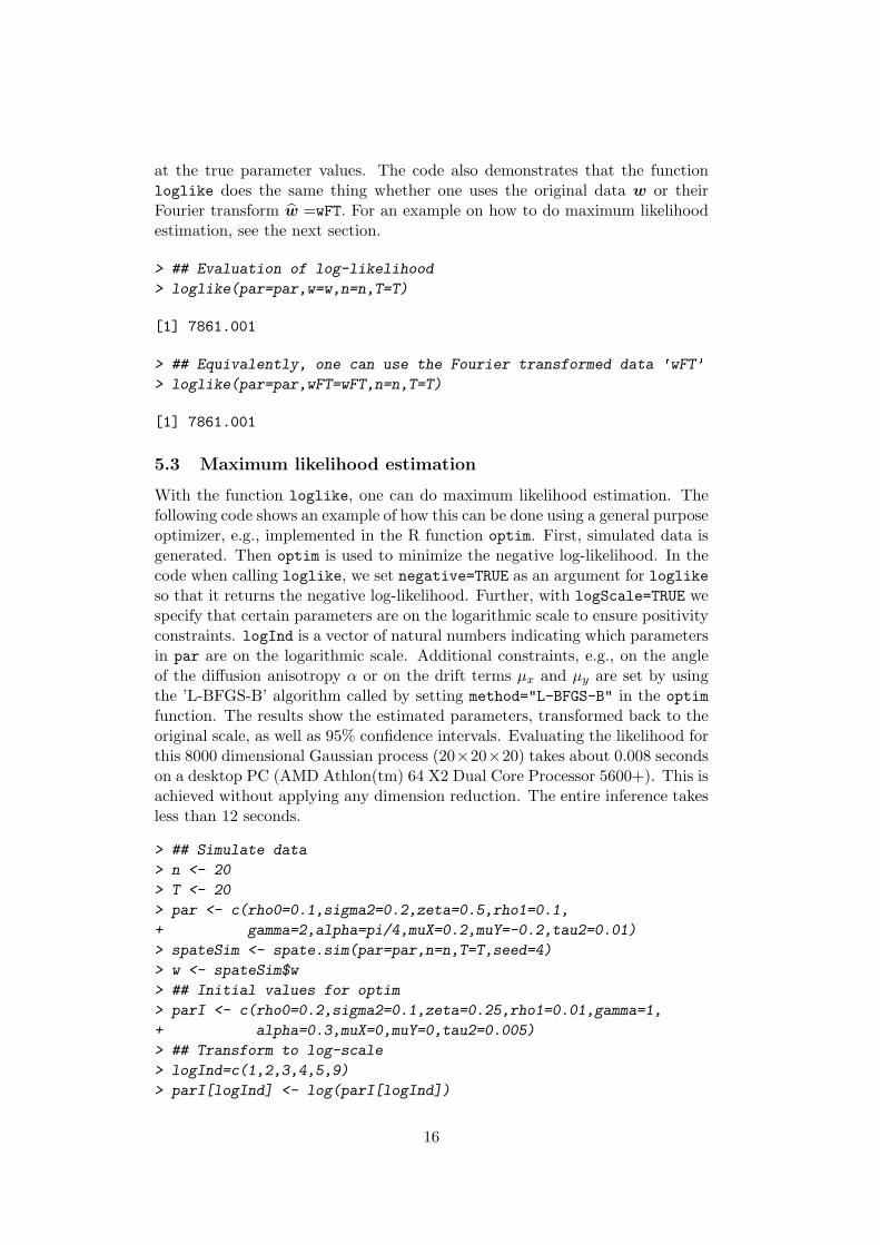
2)′.An initial state, or starting value, ξ(t1) for the dynamic model can be giventhrough the argument StartVal. The starting field needs to be a stacked vectorof lengths n2 (number of spatial points). Use as.vector() to convert a spa-tial matrix to a vector. "spateSim" objects can be plotted with the functionplot.spateSim. The code below illustrates the use of these functions. Notethat indScale=TRUE specifies that each field has its individual scale on the z-axis rather than having one common scale for all six images. Figure 7 showsone example of a simulated space-time process.

> StartVal <- rep(0,100^2)

> StartVal[75*100+75] <- 1000

> par <- c(rho0=0.05,sigma2=0.7^2,zeta=-log(0.99),rho1=0.06,

+ gamma=3,alpha=pi/4,muX=-0.1,muY=-0.1,tau2=0.00001)

> spateSim <- spate.sim(par=par,n=100,T=5,StartVal=StartVal,seed=1)

> plot(spateSim,mfrow=c(1,5),mar=c(2,2,2,2),indScale=TRUE,

+ cex.axis=1.5,cex.main=2)

20 40 60 80 100

2040

6080

100 t=1

20 40 60 80 100

2040

6080

100 t=2

20 40 60 80 100

2040

6080

100 t=3

20 40 60 80 100

2040

6080

100 t=4

20 40 60 80 100

2040

6080

100 t=5

Figure 7: Simulated spatio-temporal Gaussian process as defined in (3) and (4)

5 Inference: log-likelihood evaluation and sampling

from the full conditional

The function ffbs.spectral implements the computationally efficient Kalmanfilter and backward sampling algorithms in the spectral space for the modelspecified in (2), (3), and (4). The logical arguments lglk or BwSp controlwhether evaluation of the log-likelihood, sampling from the full conditionalof the coefficients α, or both are done. This is a wrapper function and theactual calculation is done in C. Note that either the actual observed data w

can be given or the Fourier transform w (wFT). The latter is useful if, forinstance, the log-likelihood needs to be evaluated several times given the samew. The Fourier transform is then calculated only once, instead of each time thefunction is called. loglike and sample.four.coef are wrapper functions thatcall ffbs.spectral.

5.1 Example of use of sample.four.coef

The following code illustrates the use of the function sample.four.coef. First,we simulate data w, and then we sample from the full conditional of the co-efficients [α|·] to obtain samples from the posterior of the latent process. For

14

simplicity, the parameters θ are fixed at their true values. In Figure 8, theresults are shown. In the top plot, the simulated data is displayed and in thebottom plots the mean of full conditional of the process ξ = Φα. The latteris obtained by drawing 50 samples from the full conditional [α|·], calculatingtheir mean, and applying the Fourier transform.

> ## Example of use of ✬sample.four.coef✬

> ## Simulate data

> n <- 50

> T <- 4

> par <- c(rho0=0.1,sigma2=0.2,zeta=0.5,rho1=0.1,

+ gamma=2,alpha=pi/4,muX=0.2,muY=-0.2,tau2=0.01)

> spateSim <- spate.sim(par=par,n=n,T=T,seed=4)

> w <- spateSim$w

> ## Sample from full conditional

> Nmc <- 50

> alphaS <- array(0,c(T,n*n,Nmc))

> wFT <- real.fft.TS(w,n=n,T=T)

> for(i in 1:Nmc){

+ alphaS[,,i] <- sample.four.coef(wFT=wFT,par=par,n=n,T=T,NF=n*n)

+ }

> ## Mean from full conditional

> alphaMean <- apply(alphaS,c(1,2),mean)

> xiMean <- real.fft.TS(alphaMean,n=n,T=T,inv=FALSE)

w(1) w(2) w(3) w(4)

xiPost(1) xiPost(2) xiPost(3) xiPost(4)

Figure 8: Sampling from the full conditional of the coefficients: comparison ofobserved data (top plots) and mean of full conditional of ξ (bottom plots).

5.2 Example of use of loglike

The following code provides an example of the use of loglike. We use thesame simulated data as in the previous example and evaluate the log-likelihood

15

at the true parameter values. The code also demonstrates that the functionloglike does the same thing whether one uses the original data w or theirFourier transform w =wFT. For an example on how to do maximum likelihoodestimation, see the next section.

> ## Evaluation of log-likelihood

> loglike(par=par,w=w,n=n,T=T)

[1] 7861.001

> ## Equivalently, one can use the Fourier transformed data ✬wFT✬

> loglike(par=par,wFT=wFT,n=n,T=T)

[1] 7861.001

5.3 Maximum likelihood estimation

With the function loglike, one can do maximum likelihood estimation. Thefollowing code shows an example of how this can be done using a general purposeoptimizer, e.g., implemented in the R function optim. First, simulated data isgenerated. Then optim is used to minimize the negative log-likelihood. In thecode when calling loglike, we set negative=TRUE as an argument for loglikeso that it returns the negative log-likelihood. Further, with logScale=TRUE wespecify that certain parameters are on the logarithmic scale to ensure positivityconstraints. logInd is a vector of natural numbers indicating which parametersin par are on the logarithmic scale. Additional constraints, e.g., on the angleof the diffusion anisotropy α or on the drift terms µx and µy are set by usingthe ’L-BFGS-B’ algorithm called by setting method="L-BFGS-B" in the optim

function. The results show the estimated parameters, transformed back to theoriginal scale, as well as 95% confidence intervals. Evaluating the likelihood forthis 8000 dimensional Gaussian process (20×20×20) takes about 0.008 secondson a desktop PC (AMD Athlon(tm) 64 X2 Dual Core Processor 5600+). This isachieved without applying any dimension reduction. The entire inference takesless than 12 seconds.

> ## Simulate data

> n <- 20

> T <- 20

> par <- c(rho0=0.1,sigma2=0.2,zeta=0.5,rho1=0.1,

+ gamma=2,alpha=pi/4,muX=0.2,muY=-0.2,tau2=0.01)

> spateSim <- spate.sim(par=par,n=n,T=T,seed=4)

> w <- spateSim$w

> ## Initial values for optim

> parI <- c(rho0=0.2,sigma2=0.1,zeta=0.25,rho1=0.01,gamma=1,

+ alpha=0.3,muX=0,muY=0,tau2=0.005)

> ## Transform to log-scale

> logInd=c(1,2,3,4,5,9)

> parI[logInd] <- log(parI[logInd])

16

> ## Maximum likelihood estimation using optim

> wFT <- real.fft.TS(w,n=n,T=T)

> spateMLE <- optim(par=parI,loglike,control=list(trace=TRUE,maxit=1000),

+ wFT=wFT,method="L-BFGS-B",

+ lower=c(-10,-10,-10,-10,-10,0,-0.5,-0.5,-10),

+ upper=c(10,10,10,10,10,pi/2,0.5,0.5,10),

+ negative=TRUE,logScale=TRUE,

+ logInd=c(1,2,3,4,5,9),hessian=TRUE,n=n,T=T)

iter 10 value -4963.022726

iter 20 value -5010.395816

iter 30 value -5044.942262

iter 40 value -5045.149947

final value -5045.150588

converged

> mle <- spateMLE$par

> mle[logInd] <- exp(mle[logInd])

> sd=sqrt(diag(solve(spateMLE$hessian)))

> ## Calculate confidence intervals

> MleConfInt <- data.frame(array(0,c(4,9)))

> colnames(MleConfInt) <- names(par)

> rownames(MleConfInt) <- c("True","Estimate","Lower","Upper")

> MleConfInt[1,] <- par

> MleConfInt[2,] <- mle

> MleConfInt[3,] <- spateMLE$par-2*sd

> MleConfInt[4,] <- spateMLE$par+2*sd

> MleConfInt[c(3,4),logInd] <- exp(MleConfInt[c(3,4),logInd])

> ## Results: estimates and confidence intervals

> round(MleConfInt,digits=3)

rho0 sigma2 zeta rho1 gamma alpha muX muY tau2

True 0.100 0.200 0.500 0.100 2.000 0.785 0.200 -0.200 0.010

Estimate 0.092 0.166 0.357 0.105 2.209 0.845 0.213 -0.177 0.010

Lower 0.077 0.136 0.180 0.088 1.847 0.753 0.177 -0.214 0.010

Upper 0.111 0.203 0.710 0.126 2.643 0.937 0.249 -0.139 0.011

5.4 Bayesian inference using MCMC

Using sample.four.coef and loglike a Markov chain Monte Carlo (MCMC)algorithm for drawing from the joint posterior of the latent process α, or equiv-alently ξ, and the hyper-parameters θ can be constructed.

One approach is to sample iteratively from [θ|·] using a Metropolis-Hastingsstep and from [α|·] with a Gibbs step. In many situations, α and θ can bestrongly dependent a posteriory. Consequently, if one samples successively from[θ|·] and [α|·], one can run into slow mixing properties. The reasons is that ineach step [θ|·] is constrained by the last sample of the latent process, and viceversa. To circumvent this problem, one can sample jointly from [θ,α|·]. A

17

joint proposal (θ∗,α∗) is obtained by sampling θ∗ from a Gaussian distributionwith the mean equaling the last value and an appropriately chosen covariancematrix and then sampling α∗ from [α|θ∗, ·]. The second step can be doneusing sample.four.coef. It can be shown that the acceptance probabilitythen equals

min

(1,

P [θ∗|w]

P [θ(i)|w]

), (11)

where the likelihood P [θ|w] denotes the value of the density of θ given w

evaluated at θ, and where θ∗ and θ(i) denote the proposal and the last value of θ,respectively. Since this acceptance ratio does not depend on α, the parametersθ can move faster in their parameter space. Note that P [θ|w] can be calculatedusing the function loglike.

5.4.1 Skewed Tobit model and missing data

For the transformed Tobit model (9), inference is done analogously. One justadds a Metropolis-Hastings step for the transformation parameter λ and a Gibbsstep for the censored values y(t, sl) = 0. The latter consists in simulating froma censored normal distribution with mean ξ(i)(t, sl) and variance τ2. See Sigristet al. (2012) for more details.

As said, missing values can be dealt with by using a data augmentationapproach. This means that one adds a Gibbs step consisting in simulating froma normal distribution with mean ξ(i)(t, sl) and variance (τ2)(i) for those pointswhere w(t, sl), or y(t, sl), are missing.

6 An MCMC algorithm

It is well known that the performance of MCMC algorithms can be very depen-dent on the given data, and that data specific tuning is often needed. Havingthis in mind, the function spate.mcmc implements an MCMC algorithm thatneeds as little additional fine tuning as possible. It can deal with both Gaus-sian and skewed Tobit likelihoods through the argument DataModel. Samplingis done as outlined in the previous section. I.e., the coefficients α and thehyper-parameters θ are sampled together to obtain faster mixing. Further, anadaptive algorithm (Roberts and Rosenthal, 2009) is used. This means thatthe proposal covariances RWCov for the Metropolis-Hastings step of θ are suc-cessively estimated such that an optimal acceptance rate is obtained.

The function spate.mcmc returns an object of the class "spateMCMC" with,among others, samples from the posterior of the hyper-parameters stored inthe matrix Post, the estimated proposal covariance matrix RWCov, and samplesfrom the posterior of the latent process ξ in xiPost if saveProcess=TRUE waschosen. There are plot and print functions for "spateMCMC" objects.

18

6.1 Arguments of spate.mcmc

❼ If covariates x are given, the algorithm can either sample the coefficientsβ in an additional Gibbs step from the Gaussian full conditional of thecoefficients [β|·] (FixEffMetrop=FALSE) or sample β together with θ inthe Metropolis-Hastings step (FixEffMetrop=TRUE). The latter is prefer-able since the random effects ξ and the fixed effects xβ can be stronglydependent, which can result in very slow mixing if β and ξ are samplediteratively and not jointly.

❼ The number of samples to be drawn from the Markov chain is specifiedin Nmc and the length of the burn-in in BurnIn.

❼ If the option trace=TRUE is selected, the MCMC algorithm prints run-ning status messages such as acceptance rates of the hyper-parametersand estimated remaining computing time. Additionally, if choosing plot-Trace=TRUE, running trace plots of the Markov chains are generated. Fur-ther, using SaveToFile=TRUE, the "spateMCMC" object can be successivelysaved in a directory specified through path and file.

❼ Dimension reduction can be applied by setting DimRed=TRUE and specify-ing through NFour the number of Fourier functions to be used.

❼ If the observations y are not on a grid, y can be a T × N matrix whereN(< n2) is the number of observation stations, and the coordinates of thestations can be specified in the N × 2 matrix coord. Alternatively, onecan specify through the vector Sind at which grid point each observationlies.

❼ If the boolean argument IncidenceMat equals TRUE, an incidence matrixI is constructed and the model in (10) is used. In that case, dimension re-duction needs to be done since one cannot use the fast spectral algorithmsin combination with the FFT anymore.

❼ Padding can be applied by choosing Padding=TRUE.

❼ The vector of integers indEst specifies which parameters should be esti-mated and which not. By default this equals c(1,...,9). If, for instance,one wants to fit a separable model, one can choose indEst=c(1,2,3,9)

in combination with SV=(0.2,0.1,0.25,0,0,0,0,0,0.001). The lattersets the initial values of the diffusion and drift term to zero. Since theyare not sampled, they remain at zero.

For more details and explanations on, e.g., starting values, specification ofprior distributions, selection of output for monitoring the MCMC algorithm,etc., see the help information of spate.mcmc.

6.2 Additional fine tuning

In case the MCMC algorithm still needs some fine tuning, the following argu-ments can be varied:

19

❼ the initial covariance matrix RWCov,

❼ the burn-in length BurnInCovEst before starting with the adaptive esti-mation of RWCov,

❼ the minimal number of MCMC samples NCovEst required after the burn-in for estimating RWCov.

Due to the adaptive nature of the algorithm, the initial choice of RWCov is lessimportant. However, if RWCov is overly large, the algorithm can have very smallacceptance rates with the chain barely moving at all. On the other hand, ifRWCov overly small, acceptance rates might be high, but the chain does notcover the parameter space.

If choosing adequate an RWCov turns out difficult, we propose the followingstrategy. For each hyper-parameter θi in θ, one searches for an appropriatevariance σ2

i when fixing all other parameters. This can be done by specifingthrough the argument indEst which parameters should be estimated and whichnot. For instance, if indEst=1, only for the first parameter ρ0 a Markov chainis run, and the others are fixed. Using this, an appropriate σ2

i can be foundas follows. For instance, one starts with a very low σ2

i , and then increases itsubsequently until the acceptance rate for θi, when fixing all other parameters,is at a reasonable level, say, around 0.4. After doing this for each parameter θi,RWCov=diag(σ2

i ) can be used as initial covariance matrix. Note that the goalis not to find an optimal proposal covariance matrix but rather just to get arough idea on the appropriate order of magnitude so that the algorithm is not“degenerate” from the beginning.

6.3 An example of the use of spate.mcmc

The following code illustrates the use of spate.mcmc on a simulated data set.The MCMC algorithm is run for 10000 samples with a burn-in of 2000. Theburn-in for the adaptive covariance estimation is 500 and the minimal num-ber of samples required for estimating the proposal covariance matrix of theMetropolis-Hasting step is also 500. This means that after 1000 samples, theproposal covariance matrix is first estimated. Subsequently, it is estimated ev-ery 500 samples based on the past excluding the first 500 samples from theMarkov chain. Figure 9 shows trace plots of the MCMC algorithm. The ver-tical lines represent the burn-in period, and the horizontal lines are the truevalues of the parameters. The figure shows how the mixing of the Markov chainimproves with increasing time. Note that the number of samples, 10000, is usedfor illustration. In practice, more samples are needed.

> ## Simulate data

> par <- c(rho0=0.1,sigma2=0.2,zeta=0.5,rho1=0.1,

+ gamma=2,alpha=pi/4,muX=0.2,muY=-0.2,tau2=0.01)

> spateSim <- spate.sim(par=par,n=20,T=20,seed=4)

> w <- spateSim$w

> ## This is an example to illustrate the use of the MCMC algorithm.

20

> ## In practice, more samples (Nmc) are needed for a sufficiently

> ## large effective sample size.

> spateMCMC <-spate.mcmc(y=w,x=NULL,SV=c(rho0=0.2,sigma2=0.1,

+ zeta=0.25,rho1=0.2,gamma=1,

+ alpha=0.3,muX=0,muY=0,tau2=0.005),

+ RWCov=diag(c(0.005,0.005,0.05,0.005,

+ 0.005,0.001,0.0002,0.0002,0.0002)),

+ Nmc=10000,BurnIn=2000,seed=4,NCovEst=500,

+ BurnInCovEst=500,trace=FALSE,Padding=FALSE)

> spateMCMC

Posterior of parameters:

Median 2.5 % 97.5 %

rho_0 0.09151798 0.075791669 0.10909257

sigma^2 0.17324097 0.142144435 0.22142933

zeta 0.36457843 0.112205001 0.64655163

rho_1 0.10796025 0.091442696 0.13150375

gamma 2.21058762 1.856203179 2.64283184

alpha 0.84013487 0.747082459 0.92371518

mu_x 0.21182190 0.175596745 0.25214613

mu_y -0.17956504 -0.217171052 -0.13986582

tau^2 0.01009896 0.009687484 0.01047601

Results based on 8000 MCMC samples after a burn-in of 2000 samples

The following code illustrates the use of spate.mcmc when an incidencematrix approach (see (10)) is used in combination with dimension reduction.This is the real data application used in Sigrist et al. (2012) where, roughlyspeaking, the goal is to model a spatio-temporal precipitation field. We are notshowing any results here, but we only illustrate how the function spate.mcmc iscalled. For more details, we refer to Sigrist et al. (2012). A skewed Tobit modelis used as data model. The observed data is not available on the full 100× 100grid but only at 32 observation locations. Observations are made at 720 timepoints. In the code below, y is a 720× 32 matrix, and covTS is a 2× 720× 32array containing two covariates. Sind is a vector of length 32 indicating the gridcells in which the observation stations lie. DataModel="SkewTobit" specifiesthat a skewed Tobit likelihood is used. DimRed=TRUE and NFour=29 indicatethat a reduced dimensional model consiting of 29 Fourier functions is used.By setting IncidenceMat=TRUE, we specify that an incidence matrix is used.Finally, FixEffMetrop=TRUE indicates that the coefficients of the covariates aresampled together with the hyper-parameters of the spatio-temporal model inorder to avoid slow mixing due to correlations between fixed and random effects.

> spateMCMC <- spate.mcmc(y=y,x=covTS,DataModel="SkewTobit",Sind=Sind,

+ n=100,DimRed=TRUE,NFour=29,

+ IncidenceMat=TRUE,FixEffMetrop=TRUE,Nmc=105000,

+ BurnIn=5000,Padding=TRUE,

+ NCovEst=500,BurnInCovEst=1000)

21

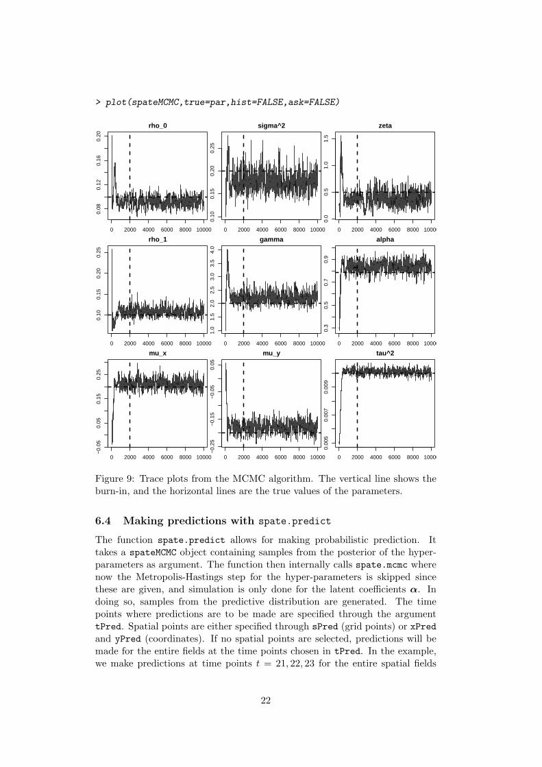
> plot(spateMCMC,true=par,hist=FALSE,ask=FALSE)

0 2000 4000 6000 8000 10000

0.08

0.12

0.16

0.20

rho_0

0 2000 4000 6000 8000 10000

0.10

0.15

0.20

0.25

sigma^2

0 2000 4000 6000 8000 10000

0.0

0.5

1.0

1.5

zeta

0 2000 4000 6000 8000 10000

0.10

0.15

0.20

0.25

rho_1

0 2000 4000 6000 8000 10000

1.0

1.5

2.0

2.5

3.0

3.5

4.0

gamma

0 2000 4000 6000 8000 10000

0.3

0.5

0.7

0.9

alpha

0 2000 4000 6000 8000 10000

−0.

050.

050.

150.

25

mu_x

0 2000 4000 6000 8000 10000

−0.

25−

0.15

−0.

050.

05

mu_y

0 2000 4000 6000 8000 10000

0.00

50.

007

0.00

9

tau^2

Figure 9: Trace plots from the MCMC algorithm. The vertical line shows theburn-in, and the horizontal lines are the true values of the parameters.

6.4 Making predictions with spate.predict

The function spate.predict allows for making probabilistic prediction. Ittakes a spateMCMC object containing samples from the posterior of the hyper-parameters as argument. The function then internally calls spate.mcmc wherenow the Metropolis-Hastings step for the hyper-parameters is skipped sincethese are given, and simulation is only done for the latent coefficients α. Indoing so, samples from the predictive distribution are generated. The timepoints where predictions are to be made are specified through the argumenttPred. Spatial points are either specified through sPred (grid points) or xPredand yPred (coordinates). If no spatial points are selected, predictions will bemade for the entire fields at the time points chosen in tPred. In the example,we make predictions at time points t = 21, 22, 23 for the entire spatial fields

22

using Nsim=100 samples. Figure 10 shows means and standard deviations ofthe predicted fields.

> ## Make predictions

> predict <- spate.predict(y=w, tPred=(21:23),

+ spateMCMC=spateMCMC, Nsim = 100,

+ BurnIn = 10, DataModel = "Normal",seed=4)

> Pmean <- apply(predict,c(1,2),mean)

> Psd <- apply(predict,c(1,2),sd)

5 10 15 20

510

1520

Mean predicted field at t=21

5 10 15 20

510

1520

Mean predicted field at t=22

5 10 15 20

510

1520

Mean predicted field at t=23

5 10 15 20

510

1520

Sd of predicted field at t=21

5 10 15 20

510

1520

Sd of predicted field at t=22

5 10 15 20

510

1520

Sd of predicted field at t=23

Figure 10: Means and standard deviations of predicted fields.

Acknowledgments

We would like to thank Martin Machler for his helpful support and advice.

References

Borgman, L., Taheri, M., and Hagan, R. (1984), “Three-dimensional frequency-domain simulations of geological variables,” in Geostatistics for Natural Re-sources Characterization, ed. Verly, G., D. Reidel, pp. 517–541.

Cressie, N. and Wikle, C. K. (2011), Statistics for spatio-temporal data, WileySeries in Probability and Statistics, John Wiley & Sons, Inc.

Dudgeon, D. E. and Mersereau, R. M. (1984), Multidimensional digital signalprocessing, Prentice-Hall.

23

Paciorek, C. J. (2007), “Bayesian smoothing with Gaussian processes usingFourier basis functions in the spectralGP package,” Journal of StatisticalSoftware, 19, 1–38.

Roberts, G. O. and Rosenthal, J. S. (2009), “Examples of adaptive MCMC,”Journal of Computational and Graphical Statistics, 18, 349–367.

Royle, J. A. and Wikle, C. K. (2005), “Efficient statistical mapping of aviancount data,” Environmental and Ecological Statistics, 12, 225–243.

Sigrist, F., Kunsch, H. R., and Stahel, W. A. (2012), “A Dynamic Non-stationary Spatio-temporal Model for Short Term Prediction of Precipita-tion,”Annals of Applied Statistics (to appear), 6, –.

Sigrist, F., Kunsch, H. R., and Stahel, W. A. (2012), “SPDE based modeling oflarge space-time data sets,” Preprint (http://arxiv.org/abs/1204.6118).

Wikle, C. K., Berliner, L. M., and Cressie, N. (1998), “Hierarchical Bayesianspace-time models,” Environmental and Ecological Statistics, 5, 117–154.

24