spatial and spatio-temporal log-gaussian cox processes...
TRANSCRIPT
Statistical Science2013, Vol. 28, No. 4, 542–563DOI: 10.1214/13-STS441© Institute of Mathematical Statistics, 2013
Spatial and Spatio-Temporal Log-GaussianCox Processes: Extending theGeostatistical ParadigmPeter J. Diggle, Paula Moraga, Barry Rowlingson and Benjamin M. Taylor
Abstract. In this paper we first describe the class of log-Gaussian Cox pro-cesses (LGCPs) as models for spatial and spatio-temporal point process data.We discuss inference, with a particular focus on the computational challengesof likelihood-based inference. We then demonstrate the usefulness of theLGCP by describing four applications: estimating the intensity surface ofa spatial point process; investigating spatial segregation in a multi-type pro-cess; constructing spatially continuous maps of disease risk from spatiallydiscrete data; and real-time health surveillance. We argue that problems ofthis kind fit naturally into the realm of geostatistics, which traditionally isdefined as the study of spatially continuous processes using spatially dis-crete observations at a finite number of locations. We suggest that a moreuseful definition of geostatistics is by the class of scientific problems that itaddresses, rather than by particular models or data formats.
Key words and phrases: Cox process, epidemiology, geostatistics, Gaus-sian process, spatial point process.
1. INTRODUCTION
Spatial statistics has been one of the most fertileareas for the development of statistical methodologyduring the second half of the twentieth century. Astriking, if slightly contrived, illustration of the paceof this development is the contrast between the 90pages of Bartlett (1975) and the 900 pages of Cressie(1991). Cressie’s book established a widely used clas-
Peter J. Diggle is Distinguished University Professor,Lancaster University Medical School, Lancaster, LA1 4YG,United Kingdom and Professor, Institute of Infection andGlobal Health, University of Liverpool, Liverpool L69 7BE,United Kingdom (e-mail: [email protected]).Paula Moraga is Research Associate, Lancaster UniversityMedical School, Lancaster, LA1 4YG, United Kingdom(e-mail: [email protected]). BarryRowlingson is Research Fellow, Lancaster UniversityMedical School, Lancaster, LA1 4YG, United Kingdom(e-mail: [email protected]). Benjamin M.Taylor is Lecturer, Lancaster University Medical School,Lancaster, LA1 4YG, United Kingdom (e-mail:[email protected]).
sification of spatial statistics into three subareas: geo-statistical data, lattice data, spatial patterns (meaningpoint patterns). Within this classification, geostatisticaldata consist of observed values of some phenomenonof interest associated with a set of spatial locationsxi : i = 1, . . . , n, where, in principle, each xi could havebeen any location x within a designated spatial regionA ⊂ R
2. Lattice data consist of observed values associ-ated with a fixed set of locations xi : i = 1, . . . , n, thatis, the phenomenon of interest exists only at those n
specific locations. Finally, in a spatial pattern the dataare a set of spatial locations xi : i = 1, . . . , n presumedto have been generated as a partial realisation of a pointprocess that is itself the object of scientific interest. Al-most 20 years later, Gelfand et al. (2010) used the sameclassification but with a different terminology focusedmore on the underlying process than on the extant data:continuous spatial variation, discrete spatial variation,and spatial point processes. With this process-basedterminology in place, continuous spatial variation im-plies a stochastic process {Y(x) :x ∈R
2}, discrete spa-tial variation implies only a finite-dimensional randomvariable, Y = {Yi : i = 1, . . . , n}, and a point patternimplies a counting measure, {dN(x) :x ∈ R
2}.542
SPATIAL AND SPATIO-TEMPORAL LOG-GAUSSIAN COX PROCESSES 543
In this paper, we argue first that the most impor-tant theoretical distinction within spatial statistics isbetween spatially continuous and spatially discretestochastic processes, and second that most natural pro-cesses are spatially continuous and should be modelledaccordingly. One consequence of this point of viewis that in many applications, maintaining a one-to-onelinkage between data formats (geostatistical, lattice,point pattern) and associated model classes (spatiallycontinuous, spatially discrete, point process) is inap-propriate. In particular, we suggest a redefinition ofgeostatistics as the collection of statistical models andmethods whose purpose is to enable predictive infer-ence about a spatially continuous, incompletely ob-served phenomenon, S(x), say.
Classically, geostatistical data Yi : i = 1, . . . , n corre-spond to noisy versions of S(xi). A standard geostatis-tical model, expressed here in hierarchical form, is thatS = {S(x) :x ∈ R
2} is a Gaussian stochastic process,whilst conditional on S , the Yi are mutually indepen-dent, Normally distributed with means S(xi) and com-mon variance τ 2. A second scenario, and the focus ofthe current paper, is when S determines the intensity,λ(x), say, of an observed Poisson point process. Anexample that we will consider in detail is a log-linearspecification, λ(x) = exp{S(x)}, where S is a Gaussianprocess. A third form is when the point process is re-duced to observations of the numbers of points Yi ineach of n regions Ai that form a partition (or subset) ofthe region of interest A. Hence, conditional on S , theYi are mutually independent, Poisson-distributed withmeans
μi =∫Ai
λ(x) dx.(1)
In the remainder of the paper we show how the log-Gaussian Cox process can be used in a range of appli-cations where S(x) is incompletely observed throughthe lens of point pattern or aggregated count data. Sec-tions 2 to 4 concern theoretical properties, inferenceand computation. Section 5 describes several appli-cations. Section 6 discusses the extension to spatio-temporal data. Section 7 gives an outline of how thisapproach to modelling incompletely observed spatialphenomena extends naturally to the joint analysis ofmultivariate spatial data when the different data ele-ments are observed at incommensurate spatial scales.Section 8 is a short, concluding discussion.
2. THE LOG-GAUSSIAN COX PROCESS
A (univariate, spatial) Cox process (Cox, 1955) is apoint process defined by the following two postulates:
CP1: � = {�(x) :x ∈ R2} is a nonnegative-valued
stochastic process;CP2: conditional on the realisation �(x) = λ(x) :
x ∈ R2, the point process is an inhomogeneous Pois-
son process with intensity λ(x).
Cox processes are natural models for point processphenomena that are environmentally driven, much lessnatural for phenomena driven primarily by interactionsamongst the points. Examples of these two situations inan epidemiological context would be the spatial distri-bution of cases of a noninfectious or infectious disease,respectively. In a noninfectious disease, the observedspatial pattern of cases results from spatial variation inthe exposure of susceptible individuals to a combina-tion of observed and unobserved risk-factors. Condi-tional on exposure, cases occur independently. In con-trast, in an infectious disease the observed pattern is atleast partially the result of infectious cases transmittingthe disease to nearby susceptibles. Notwithstandingthis phenomenological distinction, it can be difficult,or even impossible, to distinguish empirically betweenprocesses representing stochastically independent vari-ation in a heterogeneous environment and stochasticinteractions in a homogeneous environment (Bartlett,1964).
The moment properties of a Cox process are inher-ited from those of the process �(x). For example, inthe stationary case the intensity of the Cox process isequal to the expectation of �(x) and the covariancedensity of the Cox process is equal to the covariancefunction of �(x). Hence, writing λ = E[�(x)] andC(u) = Cov{�(x),�(x −u)}, the reduced second mo-ment measure or K-function (Ripley 1976, 1977) ofthe Cox process is
K(u) = πu2 + 2πλ−2∫ u
0C(v)v dv.(2)
Møller, Syversveen and Waagepetersen (1998) intro-duced the class of log-Gaussian processes (LGCPs).As the name implies, an LGCP is a Cox process with�(x) = exp{S(x)}, where S is a Gaussian process.This construction has an elegant simplicity. One of itsattractive features is that the tractability of the multi-variate Normal distribution carries over, to some ex-tent, to the associated Cox process.
In the stationary case, let μ = E[S(x)] and C(u) =σ 2r(u) = Cov{S(x), S(x−u)}. It follows from the mo-ment properties of the log-Normal distribution that theassociated LGCP has intensity λ = exp(μ+0.5σ 2) andcovariance density g(u) = λ2[exp{σ 2r(u)} − 1]. This
544 DIGGLE, MORAGA, ROWLINGSON AND TAYLOR
makes it both convenient and natural to re-parameterisethe model as
�(x) = exp{β + S(x)
},(3)
where E[S(x)] = −0.5σ 2, so that E[exp{S(x)}] = 1and λ = exp(β). This re-parameterisation gives aclean separation between first-order (mean value) andsecond-order (variation about the mean) properties.Hence, for example, if we wished to model a spatiallyvarying intensity by including one or more spatiallyindexed explanatory variables z(x), a natural first ap-proach would be to retain the stationarity of S(x) butreplace the constant intensity λ by a regression model,λ(x) = λ{z(x);β}. The resulting Cox process is nowan intensity-reweighted stationary point process (Bad-deley, Møller and Waagepetersen, 2000), which is theanalogue of a real-valued process with a spatially vary-ing mean and a stationary residual.
The definition of a multivariate LGCP is imme-diate—we simply replace the scalar-valued Gaussianprocess S(x) by a vector-valued multivariate Gaus-sian process—and its moment properties are equallytractable. For example, if S(x) is a stationary bivariateGaussian process with intensities λ1 and λ2, and cross-covariance function C12(u) = σ1σ2r12(u), the cross-covariance density of the associated Cox process isg12(u) = λ1λ2[exp{σ1σ2r12(u)} − 1].
There is an extensive literature on parametric spec-ifications for the covariance structure of real-valuedprocesses S(x); for a recent summary, see Gneitingand Guttorp (2010a). The theoretical requirement fora function C(x, y) to be a valid covariance function isthat it be positive-definite, meaning that for all positiveintegers n, any associated set of points xi ∈ R
2 : i =1, . . . , n, and any associated set of real numbers ai : i =1, . . . , n,
n∑i=1
n∑j=1
aiajC(xi, xj ) ≥ 0.(4)
Checking that (4) holds for an arbitrary candidateC(x, y) is not straightforward. In practice, we choosecovariance functions from a catalogue of parametricfamilies that are known to be valid. In the stationarycase, a widely used family is the Matérn (1960) classC(u) = σ 2r(u;φ,κ), where
r(u;φ,κ)(5)
= {2κ−1(κ)
}−1(u/φ)κKκ(u/φ) u ≥ 0.
In (5), (·) is the complete Gamma function, Kκ(·)is a modified Bessel function of order κ , and φ > 0
and κ > 0 are parameters. The parameter φ has unitsof distance, whilst κ is a dimensionless shape param-eter that determines the differentiability of the corre-sponding Gaussian process; specifically, the process isk-times mean square differentiable if κ > k. This phys-ical interpretation of κ is useful because κ is difficultto estimate empirically (Zhang, 2004), hence, a widelyused strategy is to choose between a small set of val-ues corresponding to different degrees of differentia-bility, for example, κ = 0.5,1.5 or 2.5. Estimation ofφ is more straightforward.
In summary, the LGCP is the natural analogue forpoint process data of the linear Gaussian model forreal-valued geostatistical data (Diggle and Ribeiro,2007). Like the linear Gaussian model, it lacks anymechanistic interpretation. Its principal virtue is that itprovides a flexible and relatively tractable class of em-pirical models for describing spatially correlated phe-nomena. This makes it extremely useful in a range ofapplications where the scientific focus is on spatial pre-diction rather than on testing mechanistic hypotheses.Section 5 gives several examples.
3. INFERENCE FOR LOG-GAUSSIAN COXPROCESSES
In this section we distinguish between two infer-ential targets, namely, estimation of model parame-ters and prediction of the realisations of unobservedstochastic processes. Within the Bayesian paradigm,this distinction is often blurred, because parameters aretreated as unobserved random variables and the formalmachinery of inference is the same in both cases, con-sisting of the calculation of the conditional distributionof the target given the data. However, from a scien-tific perspective parameter estimation and predictionare fundamentally different, because the former con-cerns properties of the process being modelled whereasthe latter concerns properties of a particular realisationof that process.
3.1 Parameter Estimation
For parameter estimation, we consider three ap-proaches: moment-based estimation, maximum likeli-hood estimation, and Bayesian estimation. The first ap-proach is typically very simple to implement and isuseful for the initial exploration of candidate models.The second and third are more principled, both beinglikelihood-based.
SPATIAL AND SPATIO-TEMPORAL LOG-GAUSSIAN COX PROCESSES 545
3.1.1 Moment-based estimation. In the stationarycase, moment-based estimation consists of minimis-ing a measure of the discrepancy between empiricaland theoretical second-moment properties. One classof such measures is a weighted least squares criterion,
D(θ) =∫ u0
0w(u)
{K̂(u)c − K(u; θ)c
}2du.(6)
In the intensity-re-weighted case, (6) can still be usedafter separately estimating a regression model for aspatially varying λ(x) under the working assumptionthat the data are a partial realisation of an inhomoge-neous Poisson process.
This method of estimation has an obviously ad hocquality. In particular, it is difficult to give generally ap-plicable guidance on appropriate choices for the valuesof u0 and c in (6). Because the method is intended onlyto give preliminary estimates, there is something to besaid for simply matching K̂(u) and K(u; θ) by eye.The R (R Core Team, 2013) package lgcp (Taylor etal., 2013) includes an interactive graphics function tofacilitate this.
3.1.2 Maximum likelihood estimation. The generalform of the Cox process likelihood associated with dataX = {xi ∈ A : i = 1, . . . , n} is
�(θ;X) = P(X|θ) =∫�
P(X,�|θ) d�
(7)= E�|θ
(�∗(�;X)
),
where
�∗(�;X) =n∏
i=1
�(xi)
{∫A
�(x)dx
}−n
(8)
is the likelihood for an inhomogeneous Poisson pro-cess with intensity �(x). The evaluation of (7) involvesintegration over the infinite-dimensional distribution of�. In Section 4.1 below we describe an implementationin which the continuous region of interest A is approx-imated by a finely spaced regular lattice, hence replac-ing � by a finite set of values �(gk) :k = 1, . . . ,N ,where the points g1, . . . , gN cover A. Even so, the highdimensionality of the implied integration appears topresent a formidable obstacle to analytic progress. Onesolution, easily stated but hard to implement robustlyand efficiently, is to use Monte Carlo methods.
Monte Carlo evaluation of (7) consists of approxi-mating the expectation by an empirical average oversimulated realisations of some kind. A crude MonteCarlo method would use the approximation
�MC(θ) = s−1s∑
j=1
�(θ;X,λ(j)),(9)
where λ(j) = {λ(j)(gk) :k = 1, . . . ,N} : j = 1, . . . , s
are simulated realisations of � on the set of grid-pointsgk . In practice, this is hopelessly inefficient. A betterapproach is to use an ingenious method due to Geyer(1999), as follows.
Let f (X,�; θ) denote the un-normalised joint den-sity of X and �. Then, the associated likelihood is
�(θ;X,�) = f (X,�; θ)/a(θ),(10)
where
a(θ) =∫
f (X,�; θ) d�dX(11)
is the intractable normalising constant for f (·). It fol-lows that
Eθ0
[f (X,�; θ)/f (X,�; θ0)
]=
∫ ∫f (X,�; θ)/f (X,�; θ0)
× f (X,�; θ0)
a(θ0)d�dX(12)
= 1
a(θ0)
∫f (X,�; θ) d�dX
= a(θ)/a(θ0),
where θ0 is any convenient, fixed value of θ , and Eθ0
denotes expectation when θ = θ0. However, the func-tion f (X,�; θ) in (10) is also an un-normalised con-ditional density for � given X. Under this second in-terpretation, the corresponding normalised conditionaldensity is f (X,�; θ)/a(θ |X), where
a(θ |X) =∫
f (X,�; θ) d�,(13)
and the same argument as before gives
Eθ0
[f (X,�; θ)/f (X,�; θ0)|X]
(14)= a(θ |X)/a(θ0|X).
It follows from (7), (10) and (13) that the likelihood forthe observed data, X, can be written as
�(θ;X) =∫
f (x,�; θ)
a(θ)d� = a(θ |X)/a(θ).(15)
Hence, the log-likelihood ratio between any two pa-rameter values, θ and θ0, is
L(θ;X) − L(θ0;X)
= log{a(θ |X)/a(θ)
} − log{a(θ0|X)/a(θ0)
}(16)
= log{a(θ |X)/a(θ0|X)
} − log{a(θ)/a(θ0)
}.
546 DIGGLE, MORAGA, ROWLINGSON AND TAYLOR
Substitution from (12) and (14) gives the result that
L(θ;X) − L(θ0;X)
= log Eθ0
[r(X,�, θ, θ0)|X]
(17)
− log Eθ0
[r(X,�, θ, θ0)
],
where r(X,�, θ, θ0) = f (X,�; θ)/f (X,�; θ0). Forany fixed value of θ0, a Monte Carlo approximation tothe log-likelihood, ignoring the constant term L(θ0) onthe left-hand side of (17), is therefore given by
L̂(θ) = log
{s−1
s∑j=1
r(X,λ(j), θ, θ0
)}
(18)
− log
{s−1
s∑j=1
r(X(j), λ(j), θ, θ0
)}.
The result (18) provides a Monte Carlo approxima-tion to the log-likelihood function, and therefore to themaximum likelihood estimate θ̂ , by simulating the pro-cess only at a single value, θ0. The accuracy of the ap-proximation depends on the number of simulations, s,and on how close θ0 is to θ̂ .
Note that in the second term on the right-hand sideof (18) the pairs (X(j), λ(j)) are simulated joint re-alisations of X and � at θ = θ0, whilst in the firstterm X is held fixed at the observed data and the sim-ulated realisations λ(j) are conditional on X. Condi-tional simulation of � requires Markov chain MonteCarlo (MCMC) methods, for which careful tuning isgenerally needed. We discuss computational issues, in-cluding the design of a suitable MCMC algorithm, inSection 4.
3.1.3 Bayesian estimation. One way to implementBayesian estimation would be directly to combineMonte Carlo evaluation of the likelihood with a priorfor θ . However, it turns out to be more efficient toincorporate Bayesian estimation and prediction into asingle MCMC algorithm, as described in Section 4.
3.2 Prediction
For prediction, we consider plug-in and Bayesianprediction. Suppose, quite generally, that data Y are tobe used to predict a target T under an assumed modelwith parameters θ . Then, plug-in prediction consists ofa series of probability statements within the conditionaldistribution [T |Y ; θ̂ ], where θ̂ is a point estimate of θ ,whereas Bayesian prediction replaces [T |Y ; θ̂ ] by
[T |Y ] =∫
[T |Y ; θ ][θ |Y ]dθ.(19)
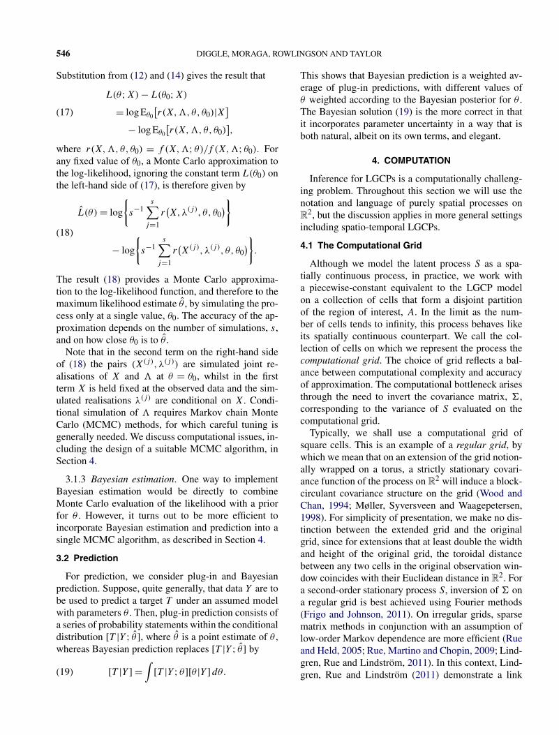
This shows that Bayesian prediction is a weighted av-erage of plug-in predictions, with different values ofθ weighted according to the Bayesian posterior for θ .The Bayesian solution (19) is the more correct in thatit incorporates parameter uncertainty in a way that isboth natural, albeit on its own terms, and elegant.
4. COMPUTATION
Inference for LGCPs is a computationally challeng-ing problem. Throughout this section we will use thenotation and language of purely spatial processes onR
2, but the discussion applies in more general settingsincluding spatio-temporal LGCPs.
4.1 The Computational Grid
Although we model the latent process S as a spa-tially continuous process, in practice, we work witha piecewise-constant equivalent to the LGCP modelon a collection of cells that form a disjoint partitionof the region of interest, A. In the limit as the num-ber of cells tends to infinity, this process behaves likeits spatially continuous counterpart. We call the col-lection of cells on which we represent the process thecomputational grid. The choice of grid reflects a bal-ance between computational complexity and accuracyof approximation. The computational bottleneck arisesthrough the need to invert the covariance matrix, ,corresponding to the variance of S evaluated on thecomputational grid.
Typically, we shall use a computational grid ofsquare cells. This is an example of a regular grid, bywhich we mean that on an extension of the grid notion-ally wrapped on a torus, a strictly stationary covari-ance function of the process on R
2 will induce a block-circulant covariance structure on the grid (Wood andChan, 1994; Møller, Syversveen and Waagepetersen,1998). For simplicity of presentation, we make no dis-tinction between the extended grid and the originalgrid, since for extensions that at least double the widthand height of the original grid, the toroidal distancebetween any two cells in the original observation win-dow coincides with their Euclidean distance in R
2. Fora second-order stationary process S, inversion of ona regular grid is best achieved using Fourier methods(Frigo and Johnson, 2011). On irregular grids, sparsematrix methods in conjunction with an assumption oflow-order Markov dependence are more efficient (Rueand Held, 2005; Rue, Martino and Chopin, 2009; Lind-gren, Rue and Lindström, 2011). In this context, Lind-gren, Rue and Lindström (2011) demonstrate a link
SPATIAL AND SPATIO-TEMPORAL LOG-GAUSSIAN COX PROCESSES 547
between models assuming a Markov dependence struc-ture and spatially continuous models whose covariancefunction belongs to a restricted subset of the Matérnclass.
4.2 Implementing Bayesian Inference, MCMC orINLA?
We now suppose that the computational grid hasbeen defined and the point process data X have beenconverted to a set of counts, Y , on the grid cells; notethat we envisage using a finely spaced grid, for whichcell-counts will typically be 0 or 1. Our goal is to usethe data Y to make inferences about the latent processS and the parameters β and θ , which, respectively, pa-rameterise the intensity of the LGCP and the covari-ance structure of S.
In the Bayesian paradigm we treat S, β and θ as ran-dom variables, assign priors to the model parameters(β, θ) and make inferential statements using the poste-rior/predictive distribution,
[S,β, θ |Y ] ∝ [Y |S,β, θ ][S|θ ][β, θ ].Two options for computation are as follows: MCMC,which generates random samples from [S,β, θ |Y ], andthe integrated nested Laplace approximation (INLA),which uses a mathematical approximation.
Taylor and Diggle (2013a) compare the performanceof MCMC and INLA for a spatial LGCP with constantexpectation β and parameters θ treated as known val-ues. In this restricted scenario, they found that MCMC,run for 100,000 iterations, delivered more accurate es-timates of predictive probabilities than INLA. How-ever, they acknowledged that “further research is re-quired in order to design better MCMC algorithms thatalso provide inference for the parameters of the latentfield”.
Approximate methods such as INLA have the ad-vantages that they produce results quickly and circum-vent the need to assess the convergence and mixingproperties of an MCMC algorithm. This makes INLAvery convenient for quick comparisons amongst multi-ple candidate models, which would be a daunting taskfor MCMC. Against this, MCMC methods are moreflexible in that extensions to standard classes of mod-els can usually be accommodated with only a modestamount of coding effort. Also, an important consider-ation in some applications is that the currently avail-able software implementation of INLA is limited tothe evaluation of predictive distributions for univari-ate, or, at best, low-dimensional, components of theunderlying model, whereas MCMC provides direct ac-
cess to joint posterior/predictive distributions of non-linear functions of the parameters and of the latent pro-cess S. Mixing INLA and MCMC can therefore bea good overall computational strategy. For example,Haran and Tierney (2012) use a heavy-tailed approx-imation similar in spirit to INLA to construct efficientMCMC proposal schemes.
4.2.1 Markov Chain Monte Carlo inference for log-Gaussian Cox processes. MCMC methods generatesamples from a Markov chain whose stationary distri-bution is the target of interest, in our case [S,β, θ |Y ].Such samples are inherently dependent but, subject tocareful checking of mixing and convergence proper-ties, their empirical distribution is an unbiased estimateof the target, and, in principle, the associated MonteCarlo error can be made arbitrarily small by using asufficiently long run of the chain. In the current con-text, we follow Møller, Syversveen and Waagepetersen(1998) and Brix and Diggle (2001) in using a standard-ised version of S, denoted , and transform θ to thelog-scale, so that the MCMC algorithm operates on thewhole of Rd , rather than on a restricted subset. We de-note the ith sample from the chain by ζ (i) and writeπ(ζ |Y) for the target distribution.
The aim in designing MCMC algorithms for anyspecific class of problems is to achieve faster con-vergence and better mixing than would be obtainedby generic off-the-shelf methods. Gilks, Richardsonand Spiegelhalter (1995) and Gamerman and Lopes(2006) give overviews of the extensive literature onthis topic. We focus our discussion on the Metropolis-Hastings (MH) algorithm, which includes as a spe-cial case the popular Gibbs sampler (Metropolis etal., 1953; Hastings, 1970; Geman and Geman, 1984;Spiegelhalter, Thomas and Best, 1999). In order touse the MH algorithm, we require a proposal density,q(·|ζ (i−1)). At the ith iteration of the algorithm, wesample a candidate, ζ (i∗), from q(·), and set ζ (i) = ζ (i∗)
with probability
min{
1,π(ζ (i∗)|Y)
π(ζ (i−1)|Y)
q(ζ (i−1)|ζ (i∗))
q(ζ (i∗)|ζ (i−1))
},
otherwise set ζ (i) = ζ (i−1). The choice of q(·) is crit-ical. Previous research on inferential methods for spa-tial and spatio-temporal log-Gaussian Cox processeshas advocated the Metropolis-adjusted Langevin al-gorithm (MALA), which mimics a Langevin diffu-sion on the target of interest; see Roberts and Tweedie(1996), Møller, Syversveen and Waagepetersen (1998)and Brix and Diggle (2001); note also Brix and Diggle(2003) and Taylor and Diggle (2013b). Alternatives to
548 DIGGLE, MORAGA, ROWLINGSON AND TAYLOR
MH include Hamiltonian Monte Carlo methods, as dis-cussed in Girolami and Calderhead (2011).
The Metropolis-adjusted Langevin algorithm ex-ploits gradient information to identify efficient pro-posals. The algorithms in this article make use of a“pre-conditioning matrix”, � (Girolami and Calder-head, 2011), to define the proposal
q(ζ (i∗)|ζ (i−1))= N
[ζ (i∗);(20)
ζ (i−1) + h2
2�∇ log
{π
(ζ (i−1)|Y )}
, h2�
],
where h is a scaling constant. Ideally, � should be thenegative inverse of the Fisher information matrix eval-uated at the maximum likelihood estimate of ζ , thatis, �opt = {−E[I(ζ̂ )]}−1 where I is the observed in-formation. However, this matrix is massive, dense andintractable. In practice, we can obtain an efficient al-gorithm by choosing � to be an approximation of �optand further by changing h during the course of the al-gorithm using adaptive MCMC (Andrieu and Thoms,2008; Roberts and Rosenthal, 2007). In MALA algo-rithms, h can be tuned adaptively to achieve an approx-imately optimal acceptance rate of 0.574 (Roberts andRosenthal, 2001).
Since the gradient of logπ with respect to θ can beboth difficult to compute and computationally costly,we instead suggest a random walk proposal for the θ -component of ζ . In the examples described in Section 5we used the following overall proposal:
q(ζ (i∗)|ζ (i−1))
= N
⎡⎢⎢⎢⎢⎢⎣ζ (i∗);
(21) ⎛⎜⎜⎜⎜⎜⎝
(i−1) + h2h2
2�
∂ log{π
(ζ (i−1)|Y )}∂
β(i−1) + h2h2β
2�β
∂ log{π
(ζ (i−1)|Y )}∂β
θ(i−1)
⎞⎟⎟⎟⎟⎟⎠ ,
h2
⎛⎜⎝
h2� 0 0
0 h2β�β 0
0 0 ch2θ�θ
⎞⎟⎠
⎤⎥⎥⎥⎥⎥⎦ .
In (21), � is an approximation to {−E[I(̂)]}−1, andsimilarly for �β and �θ . The constants h2
, h2β and
h2θ are the approximately optimal scalings for Gaus-
sian targets explored by the Gaussian random walk orMALA proposals (Roberts and Rosenthal, 2001); theseare, respectively, 1.652/dim()1/3, 1.652/dim(β)1/3
and 2.382/dim(θ), where dim is the dimension.The acceptance rate for a random walk proposal is
often tuned to around 0.234, which is optimal for aGaussian target in the limit as the dimension of the tar-get goes to infinity. At each step in our algorithm, wejointly propose new values for (S,β) and for θ using,respectively, a MALA and a random walk componentin the overall proposal, but we also seek to maintain anacceptance rate of 0.574 to achieve optimality for theMALA parts of the proposal. As a compromise, in ourproposal we scale the matrix �θ by a constant factorc and the proposal covariance matrix by a single adap-tive h. In the examples described in Section 5 we useda value of c = 0.4, which appears to work well acrossa range of scenarios.
5. APPLICATIONS
5.1 Smoothing a Spatial Point Pattern
The intensity, λ(x), of an inhomogeneous spatialpoint process is the unique nonnegative valued functionsuch that the expected number of points of the process,called events, that fall within any spatial region B is
μ(B) =∫B
λ(x) dx.(22)
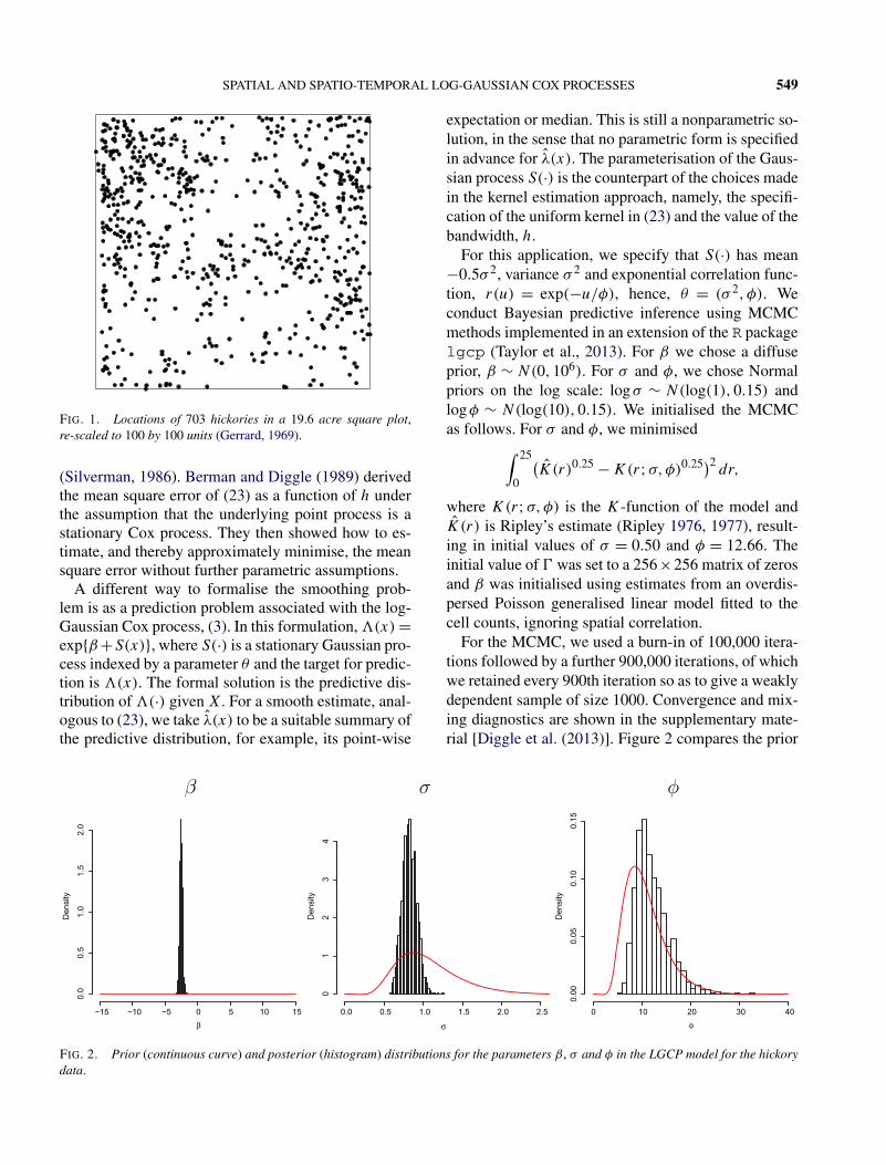
Suppose that we wish to estimate λ(x) from a partialrealisation consisting of all of the events of the processthat fall within a region A, hence, X = {xi ∈ A : i =1, . . . , n}. Figure 1 shows an example in which thedata are the locations of 703 hickory trees in a 19.6acre (281.6 by 281.6 metre) square region A (Gerrard,1969), which we have re-scaled to be of dimension 100by 100.
An intuitively reasonable class of estimators for λ(x)
is obtained by counting the number of events that liewithin some fixed distance, h, say, of x and dividing byπh2 or, to allow for edge-effects, by the area, B(x, t),of the intersection of A and a circular disc with centrex and radius h, hence,
λ̃(x;h) = B(x;h)−1n∑
i=1
I(‖x − xi‖ ≤ h
).(23)
This estimate is, in essence, a simple form of bivari-ate kernel smoothing with a uniform kernel function
SPATIAL AND SPATIO-TEMPORAL LOG-GAUSSIAN COX PROCESSES 549
FIG. 1. Locations of 703 hickories in a 19.6 acre square plot,re-scaled to 100 by 100 units (Gerrard, 1969).
(Silverman, 1986). Berman and Diggle (1989) derivedthe mean square error of (23) as a function of h underthe assumption that the underlying point process is astationary Cox process. They then showed how to es-timate, and thereby approximately minimise, the meansquare error without further parametric assumptions.
A different way to formalise the smoothing prob-lem is as a prediction problem associated with the log-Gaussian Cox process, (3). In this formulation, �(x) =exp{β +S(x)}, where S(·) is a stationary Gaussian pro-cess indexed by a parameter θ and the target for predic-tion is �(x). The formal solution is the predictive dis-tribution of �(·) given X. For a smooth estimate, anal-ogous to (23), we take λ̂(x) to be a suitable summary ofthe predictive distribution, for example, its point-wise
expectation or median. This is still a nonparametric so-lution, in the sense that no parametric form is specifiedin advance for λ̂(x). The parameterisation of the Gaus-sian process S(·) is the counterpart of the choices madein the kernel estimation approach, namely, the specifi-cation of the uniform kernel in (23) and the value of thebandwidth, h.
For this application, we specify that S(·) has mean−0.5σ 2, variance σ 2 and exponential correlation func-tion, r(u) = exp(−u/φ), hence, θ = (σ 2, φ). Weconduct Bayesian predictive inference using MCMCmethods implemented in an extension of the R packagelgcp (Taylor et al., 2013). For β we chose a diffuseprior, β ∼ N(0,106). For σ and φ, we chose Normalpriors on the log scale: logσ ∼ N(log(1),0.15) andlogφ ∼ N(log(10),0.15). We initialised the MCMCas follows. For σ and φ, we minimised∫ 25
0
(K̂(r)0.25 − K(r;σ,φ)0.25)2
dr,
where K(r;σ,φ) is the K-function of the model andK̂(r) is Ripley’s estimate (Ripley 1976, 1977), result-ing in initial values of σ = 0.50 and φ = 12.66. Theinitial value of was set to a 256×256 matrix of zerosand β was initialised using estimates from an overdis-persed Poisson generalised linear model fitted to thecell counts, ignoring spatial correlation.
For the MCMC, we used a burn-in of 100,000 itera-tions followed by a further 900,000 iterations, of whichwe retained every 900th iteration so as to give a weaklydependent sample of size 1000. Convergence and mix-ing diagnostics are shown in the supplementary mate-rial [Diggle et al. (2013)]. Figure 2 compares the prior
FIG. 2. Prior (continuous curve) and posterior (histogram) distributions for the parameters β , σ and φ in the LGCP model for the hickorydata.
550 DIGGLE, MORAGA, ROWLINGSON AND TAYLOR
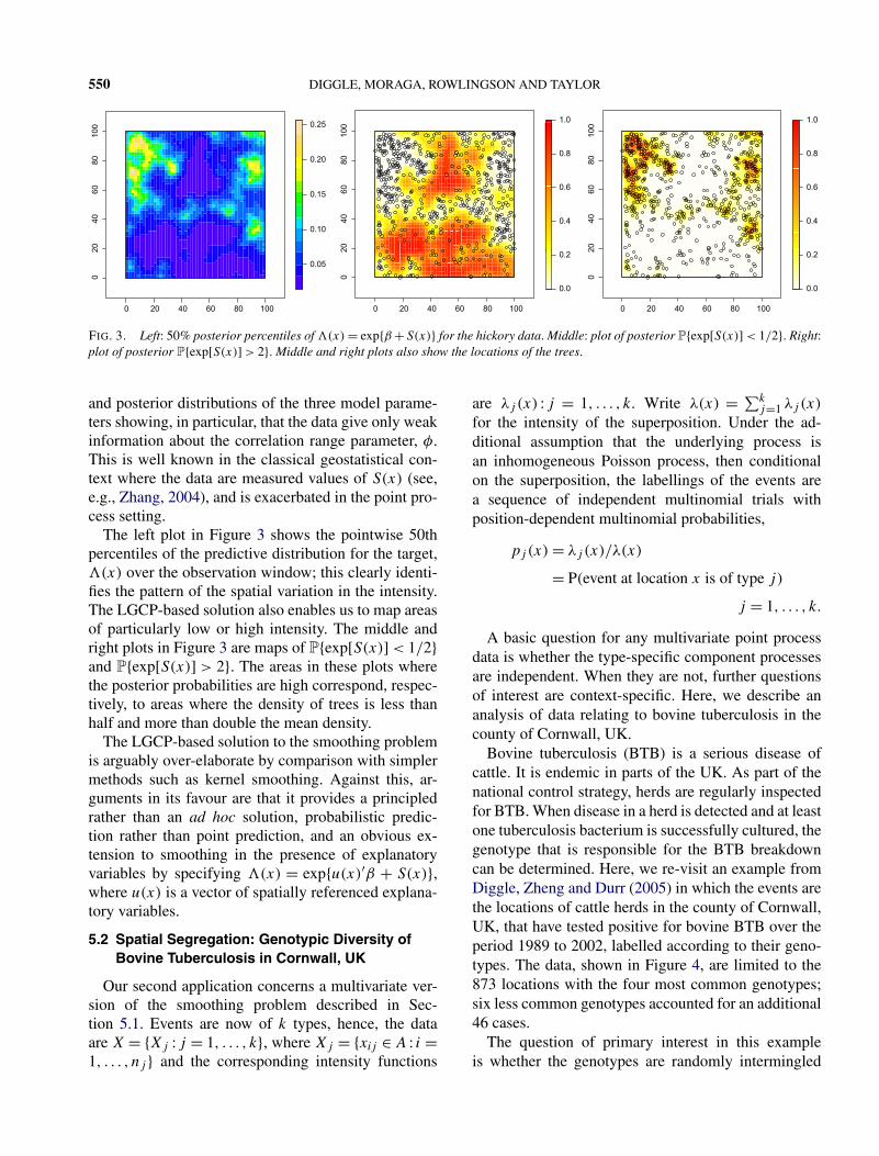
FIG. 3. Left: 50% posterior percentiles of �(x) = exp{β +S(x)} for the hickory data. Middle: plot of posterior P{exp[S(x)] < 1/2}. Right:plot of posterior P{exp[S(x)] > 2}. Middle and right plots also show the locations of the trees.
and posterior distributions of the three model parame-ters showing, in particular, that the data give only weakinformation about the correlation range parameter, φ.This is well known in the classical geostatistical con-text where the data are measured values of S(x) (see,e.g., Zhang, 2004), and is exacerbated in the point pro-cess setting.
The left plot in Figure 3 shows the pointwise 50thpercentiles of the predictive distribution for the target,�(x) over the observation window; this clearly identi-fies the pattern of the spatial variation in the intensity.The LGCP-based solution also enables us to map areasof particularly low or high intensity. The middle andright plots in Figure 3 are maps of P{exp[S(x)] < 1/2}and P{exp[S(x)] > 2}. The areas in these plots wherethe posterior probabilities are high correspond, respec-tively, to areas where the density of trees is less thanhalf and more than double the mean density.
The LGCP-based solution to the smoothing problemis arguably over-elaborate by comparison with simplermethods such as kernel smoothing. Against this, ar-guments in its favour are that it provides a principledrather than an ad hoc solution, probabilistic predic-tion rather than point prediction, and an obvious ex-tension to smoothing in the presence of explanatoryvariables by specifying �(x) = exp{u(x)′β + S(x)},where u(x) is a vector of spatially referenced explana-tory variables.
5.2 Spatial Segregation: Genotypic Diversity ofBovine Tuberculosis in Cornwall, UK
Our second application concerns a multivariate ver-sion of the smoothing problem described in Sec-tion 5.1. Events are now of k types, hence, the dataare X = {Xj : j = 1, . . . , k}, where Xj = {xij ∈ A : i =1, . . . , nj } and the corresponding intensity functions
are λj (x) : j = 1, . . . , k. Write λ(x) = ∑kj=1 λj (x)
for the intensity of the superposition. Under the ad-ditional assumption that the underlying process isan inhomogeneous Poisson process, then conditionalon the superposition, the labellings of the events area sequence of independent multinomial trials withposition-dependent multinomial probabilities,
pj (x) = λj (x)/λ(x)
= P(event at location x is of type j)
j = 1, . . . , k.
A basic question for any multivariate point processdata is whether the type-specific component processesare independent. When they are not, further questionsof interest are context-specific. Here, we describe ananalysis of data relating to bovine tuberculosis in thecounty of Cornwall, UK.
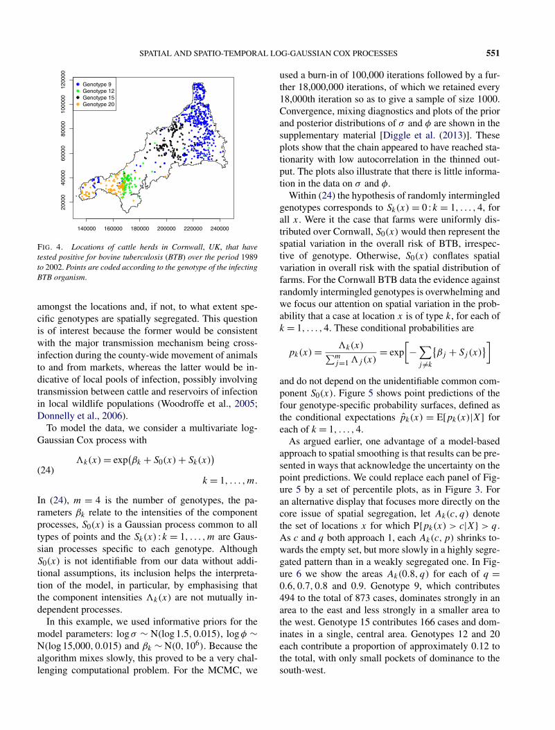
Bovine tuberculosis (BTB) is a serious disease ofcattle. It is endemic in parts of the UK. As part of thenational control strategy, herds are regularly inspectedfor BTB. When disease in a herd is detected and at leastone tuberculosis bacterium is successfully cultured, thegenotype that is responsible for the BTB breakdowncan be determined. Here, we re-visit an example fromDiggle, Zheng and Durr (2005) in which the events arethe locations of cattle herds in the county of Cornwall,UK, that have tested positive for bovine BTB over theperiod 1989 to 2002, labelled according to their geno-types. The data, shown in Figure 4, are limited to the873 locations with the four most common genotypes;six less common genotypes accounted for an additional46 cases.
The question of primary interest in this exampleis whether the genotypes are randomly intermingled
SPATIAL AND SPATIO-TEMPORAL LOG-GAUSSIAN COX PROCESSES 551
FIG. 4. Locations of cattle herds in Cornwall, UK, that havetested positive for bovine tuberculosis (BTB) over the period 1989to 2002. Points are coded according to the genotype of the infectingBTB organism.
amongst the locations and, if not, to what extent spe-cific genotypes are spatially segregated. This questionis of interest because the former would be consistentwith the major transmission mechanism being cross-infection during the county-wide movement of animalsto and from markets, whereas the latter would be in-dicative of local pools of infection, possibly involvingtransmission between cattle and reservoirs of infectionin local wildlife populations (Woodroffe et al., 2005;Donnelly et al., 2006).
To model the data, we consider a multivariate log-Gaussian Cox process with
�k(x) = exp(βk + S0(x) + Sk(x)
)(24)
k = 1, . . . ,m.
In (24), m = 4 is the number of genotypes, the pa-rameters βk relate to the intensities of the componentprocesses, S0(x) is a Gaussian process common to alltypes of points and the Sk(x) :k = 1, . . . ,m are Gaus-sian processes specific to each genotype. AlthoughS0(x) is not identifiable from our data without addi-tional assumptions, its inclusion helps the interpreta-tion of the model, in particular, by emphasising thatthe component intensities �k(x) are not mutually in-dependent processes.
In this example, we used informative priors for themodel parameters: logσ ∼ N(log 1.5,0.015), logφ ∼N(log 15,000,0.015) and βk ∼ N(0,106). Because thealgorithm mixes slowly, this proved to be a very chal-lenging computational problem. For the MCMC, we
used a burn-in of 100,000 iterations followed by a fur-ther 18,000,000 iterations, of which we retained every18,000th iteration so as to give a sample of size 1000.Convergence, mixing diagnostics and plots of the priorand posterior distributions of σ and φ are shown in thesupplementary material [Diggle et al. (2013)]. Theseplots show that the chain appeared to have reached sta-tionarity with low autocorrelation in the thinned out-put. The plots also illustrate that there is little informa-tion in the data on σ and φ.
Within (24) the hypothesis of randomly intermingledgenotypes corresponds to Sk(x) = 0 :k = 1, . . . ,4, forall x. Were it the case that farms were uniformly dis-tributed over Cornwall, S0(x) would then represent thespatial variation in the overall risk of BTB, irrespec-tive of genotype. Otherwise, S0(x) conflates spatialvariation in overall risk with the spatial distribution offarms. For the Cornwall BTB data the evidence againstrandomly intermingled genotypes is overwhelming andwe focus our attention on spatial variation in the prob-ability that a case at location x is of type k, for each ofk = 1, . . . ,4. These conditional probabilities are
pk(x) = �k(x)∑mj=1 �j(x)
= exp[− ∑
j �=k
{βj + Sj (x)
}]
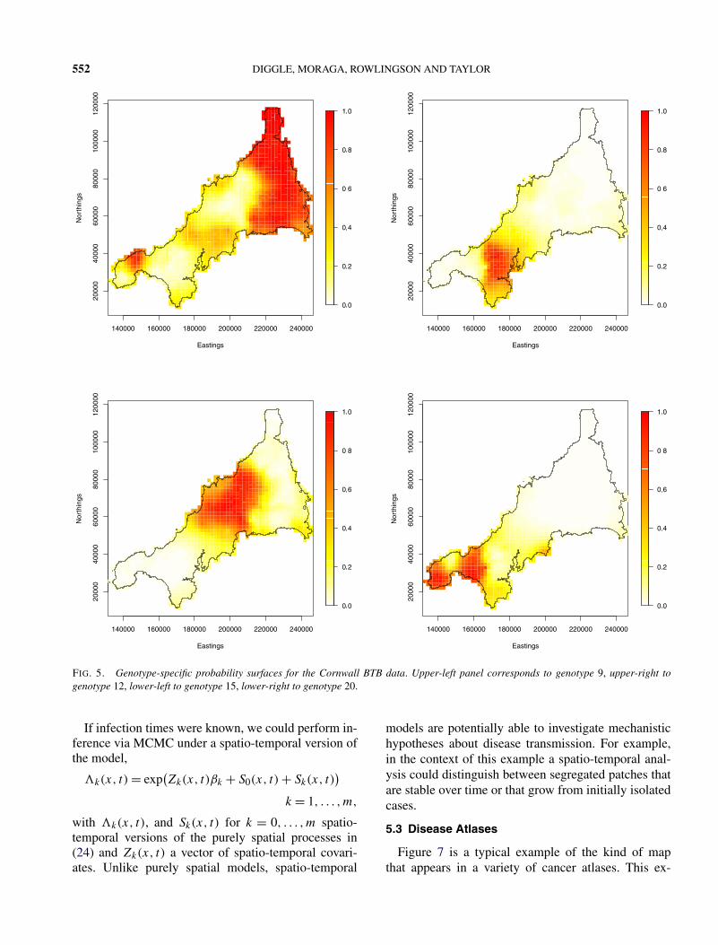
and do not depend on the unidentifiable common com-ponent S0(x). Figure 5 shows point predictions of thefour genotype-specific probability surfaces, defined asthe conditional expectations p̂k(x) = E[pk(x)|X] foreach of k = 1, . . . ,4.
As argued earlier, one advantage of a model-basedapproach to spatial smoothing is that results can be pre-sented in ways that acknowledge the uncertainty on thepoint predictions. We could replace each panel of Fig-ure 5 by a set of percentile plots, as in Figure 3. Foran alternative display that focuses more directly on thecore issue of spatial segregation, let Ak(c, q) denotethe set of locations x for which P{pk(x) > c|X} > q .As c and q both approach 1, each Ak(c,p) shrinks to-wards the empty set, but more slowly in a highly segre-gated pattern than in a weakly segregated one. In Fig-ure 6 we show the areas Ak(0.8, q) for each of q =0.6,0.7,0.8 and 0.9. Genotype 9, which contributes494 to the total of 873 cases, dominates strongly in anarea to the east and less strongly in a smaller area tothe west. Genotype 15 contributes 166 cases and dom-inates in a single, central area. Genotypes 12 and 20each contribute a proportion of approximately 0.12 tothe total, with only small pockets of dominance to thesouth-west.
552 DIGGLE, MORAGA, ROWLINGSON AND TAYLOR
FIG. 5. Genotype-specific probability surfaces for the Cornwall BTB data. Upper-left panel corresponds to genotype 9, upper-right togenotype 12, lower-left to genotype 15, lower-right to genotype 20.
If infection times were known, we could perform in-ference via MCMC under a spatio-temporal version ofthe model,
�k(x, t) = exp(Zk(x, t)βk + S0(x, t) + Sk(x, t)
)k = 1, . . . ,m,
with �k(x, t), and Sk(x, t) for k = 0, . . . ,m spatio-temporal versions of the purely spatial processes in(24) and Zk(x, t) a vector of spatio-temporal covari-ates. Unlike purely spatial models, spatio-temporal
models are potentially able to investigate mechanistichypotheses about disease transmission. For example,in the context of this example a spatio-temporal anal-ysis could distinguish between segregated patches thatare stable over time or that grow from initially isolatedcases.
5.3 Disease Atlases
Figure 7 is a typical example of the kind of mapthat appears in a variety of cancer atlases. This ex-
SPATIAL AND SPATIO-TEMPORAL LOG-GAUSSIAN COX PROCESSES 553
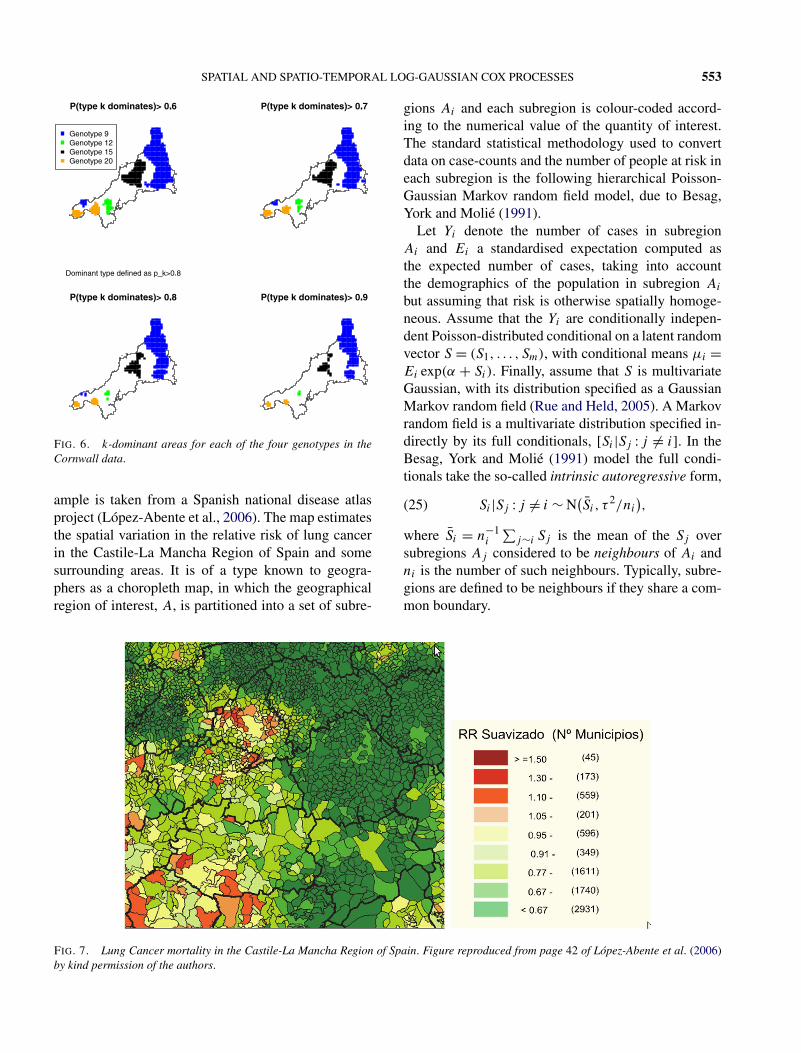
FIG. 6. k-dominant areas for each of the four genotypes in theCornwall data.
ample is taken from a Spanish national disease atlasproject (López-Abente et al., 2006). The map estimatesthe spatial variation in the relative risk of lung cancerin the Castile-La Mancha Region of Spain and somesurrounding areas. It is of a type known to geogra-phers as a choropleth map, in which the geographicalregion of interest, A, is partitioned into a set of subre-
gions Ai and each subregion is colour-coded accord-ing to the numerical value of the quantity of interest.The standard statistical methodology used to convertdata on case-counts and the number of people at risk ineach subregion is the following hierarchical Poisson-Gaussian Markov random field model, due to Besag,York and Molié (1991).
Let Yi denote the number of cases in subregionAi and Ei a standardised expectation computed asthe expected number of cases, taking into accountthe demographics of the population in subregion Ai
but assuming that risk is otherwise spatially homoge-neous. Assume that the Yi are conditionally indepen-dent Poisson-distributed conditional on a latent randomvector S = (S1, . . . , Sm), with conditional means μi =Ei exp(α + Si). Finally, assume that S is multivariateGaussian, with its distribution specified as a GaussianMarkov random field (Rue and Held, 2005). A Markovrandom field is a multivariate distribution specified in-directly by its full conditionals, [Si |Sj : j �= i]. In theBesag, York and Molié (1991) model the full condi-tionals take the so-called intrinsic autoregressive form,
Si |Sj : j �= i ∼ N(S̄i , τ
2/ni
),(25)
where S̄i = n−1i
∑j∼i Sj is the mean of the Sj over
subregions Aj considered to be neighbours of Ai andni is the number of such neighbours. Typically, subre-gions are defined to be neighbours if they share a com-mon boundary.
FIG. 7. Lung Cancer mortality in the Castile-La Mancha Region of Spain. Figure reproduced from page 42 of López-Abente et al. (2006)by kind permission of the authors.
554 DIGGLE, MORAGA, ROWLINGSON AND TAYLOR
An alternative approach is to model the locationsof individual cancer cases as an LGCP with intensity�(x) = d(x)R(x), where d(x) represents populationdensity, assumed known, and R(x) denotes diseaserisk, R(x) = exp{S(x)}. Conditional on R(·), case-counts in subregions Ai are independent and Poisson-distributed with means
μi =∫Ai
d(x)R(x)dx.
This approach leads to spatially smooth risk-mapswhose interpretation is independent of the particularpartition of A into subregions Ai . This is an importantconsideration when the Ai differ greatly in size andshape, as the definition of neighbours in an MRF modelthen becomes problematic; see, for example, Wall(2004). Fitting a spatially continuous model also hasthe potential to add information to an analysis of ag-gregated data, for example, when data on environmen-tal risk-factors are available at high spatial resolution.A caveat is that the population density may only beavailable in the form of small-area population counts,implying a piece-wise constant surface d(x) that canonly be a convenient fiction. Note, however, that spa-tially continuous modelled population density mapshave been constructed and are freely available; see,for example, http://sedac.ciesin.columbia.edu/data/set/gpw-v3-population-density.
For the Spanish lung cancer data, we have covariateinformation available at small-area, which we incorpo-rate by fitting the model
�(x) = d(x) exp{z(x)′β + S(x)
},(26)
treating the covariate surfaces z(x) as piece-wise con-stant.
For Bayesian inference under the continuous model(26) we follow Li et al. (2012) by adding standard dataaugmentation techniques to the MCMC fitting algo-rithm described earlier. Recall that for computationalpurposes, we perform all calculations on a fine grid,treating the cell counts in each grid cell as Poissondistributed conditional on the latent process S(·). Pro-vided the computational grid is fine enough, each Ai
can be approximated by the union of a set of grid cells,and we can use a grid-based Gibbs sampling strat-egy, repeatedly sampling first from [S,β, θ |N,Y+] =[S,β, θ |N ] and then from [N |S,β, θ,Y+], where N
are the cell counts on the computational grid, Y+ ={Yi = ∑
x∈AiN(x) : i = 1, . . . ,m} and θ parameterises
the covariance structure of S. Sampling from the firstof these densities can be achieved using a Metropolis-Hastings update as discussed in Section 4. The second
density is a multinomial distribution and poses no dif-ficulty.
Our priors for this example were as follows: logσ ∼N(log 1,0.3), logφ ∼ N(log 3000,0.15) and β ∼MVN(0,106I ). For the MCMC algorithm, we useda burn-in of 100,000 iterations followed by a fur-ther 18,000,000 iterations, of which we retained every18,000th iteration so as to give a sample of size 1000.Convergence, mixing diagnostics and plots of the priorand posterior distributions of σ and φ are shown inthe supplementary material [Diggle et al. (2013)]. Asin the Cornwall BTB analysis, these plots indicatedconvergence to the stationary distribution and low au-tocorrelation in the thinned output.
In the analysis reported here, we base our offseton modelled population data at 100 metre resolu-tion obtained from the European Environment Agen-cy; see http://www.eea.europa.eu/data-and-maps/data/population-density-disaggregated-with-corine- land-cover-2000-2. We projected this very fine populationinformation onto our computational grid, which con-sisted of cells 3100 × 3100 metres in dimension. Weused an exponential model for the covariance functionof S(·) and estimated its parameters (posterior medianand 95% credible interval) to be σ = 1.57 (1.45,1.71)
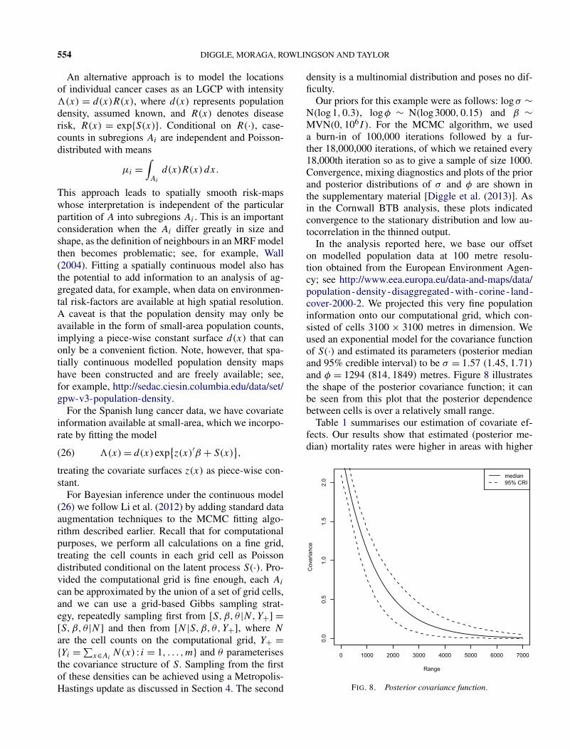
and φ = 1294 (814,1849) metres. Figure 8 illustratesthe shape of the posterior covariance function; it canbe seen from this plot that the posterior dependencebetween cells is over a relatively small range.
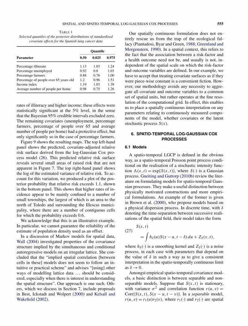
Table 1 summarises our estimation of covariate ef-fects. Our results show that estimated (posterior me-dian) mortality rates were higher in areas with higher
FIG. 8. Posterior covariance function.
SPATIAL AND SPATIO-TEMPORAL LOG-GAUSSIAN COX PROCESSES 555
TABLE 1Selected quantiles of the posterior distributions of standardised
covariate effects for the Spanish lung cancer data
Quantile
Parameter 0.50 0.025 0.975
Percentage illiterate 1.13 1.03 1.24Percentage unemployed 0.92 0.8 1.03Percentage farmers 0.88 0.76 1.00Percentage of people over 65 years old 1.2 0.96 1.51Income index 1.19 1.03 1.39Average number of people per home 0.98 0.75 1.26
rates of illiteracy and higher income; these effects werestatistically significant at the 5% level, in the sensethat the Bayesian 95% credible intervals excluded zero.The remaining covariates (unemployment, percentagefarmers, percentage of people over 65 and averagenumber of people per home) had a protective effect, butonly significantly so in the case of percentage farmers.
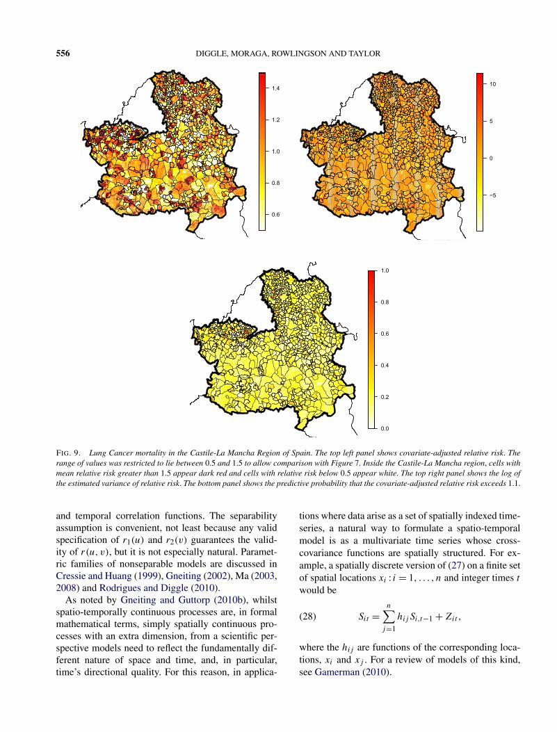
Figure 9 shows the resulting maps. The top left-handpanel shows the predicted, covariate-adjusted relativerisk surface derived from the log-Gaussian Cox pro-cess model (26). This predicted relative risk surfacereveals several small areas of raised risk that are notapparent in Figure 7. The top right-hand panel showsthe log of the estimated variance of relative risk. To ac-count for this variation, we produced a plot of the pos-terior probability that relative risk exceeds 1.1, shownin the bottom panel. This shows that higher rates of in-cidence appear to be mainly confined to a number ofsmall townships, the largest of which is an area to thenorth of Toledo and surrounding the Illescas munici-pality, where there are a number of contiguous cellsfor which the probability exceeds 0.6.
We acknowledge that this is an illustrative example.In particular, we cannot guarantee the reliability of theestimate of population density used as an offset.
In a discussion of Markov models for spatial data,Wall (2004) investigated properties of the covariancestructure implied by the simultaneous and conditionalautoregressive models on an irregular lattice. She con-cluded that the “implied spatial correlation [betweencells in these] models does not seem to follow an in-tuitive or practical scheme” and advises “[using] otherways of modelling lattice data . . . should be consid-ered, especially when there is interest in understandingthe spatial structure”. Our approach is one such. Oth-ers, which we discuss in Section 7, include proposalsin Best, Ickstadt and Wolpert (2000) and Kelsall andWakefield (2002).
Our spatially continuous formulation does not en-tirely rescue us from the trap of the ecological fal-lacy (Piantadosi, Byar and Green, 1988; Greenland andMorgenstern, 1990). In a spatial context, this refers tothe fact that the association between a risk-factor anda health outcome need not be, and usually is not, in-dependent of the spatial scale on which the risk-factorand outcome variables are defined. In our example, wehave to accept that treating covariate surfaces as if theywere piece-wise constant is a convenient fiction. How-ever, our methodology avoids any necessity to aggre-gate all covariate and outcome variables to a commonset of spatial units, but rather operates at the fine reso-lution of the computational grid. In effect, this enablesus to place a spatially continuous interpretation on anyparameters relating to continuously measured compo-nents of the model, whether covariates or the latentstochastic process S(x).
6. SPATIO-TEMPORAL LOG-GAUSSIAN COXPROCESSES
6.1 Models
A spatio-temporal LGCP is defined in the obviousway, as a spatio-temporal Poisson point process condi-tional on the realisation of a stochastic intensity func-tion �(x, t) = exp{S(x, t)}, where S(·) is a Gaussianprocess. Gneiting and Guttorp (2010b) review the liter-ature on formulating models for spatio-temporal Gaus-sian processes. They make a useful distinction betweenphysically motivated constructions and more empiri-cal formulations. An example of the former is givenin Brown et al. (2000), who propose models based ona physical dispersion process. In discrete time, with δ
denoting the time-separation between successive reali-sations of the spatial field, their model takes the form
S(x, t)(27)
=∫
hδ(u)S(x − u, t − δ) du + Zδ(x, t),
where hδ(·) is a smoothing kernel and Zδ(·) is a noiseprocess, in each case with parameters that depend onthe value of δ in such a way as to give a consistentinterpretation in the spatio-temporally continuous limitas δ → 0.
Amongst empirical spatio-temporal covariance mod-els, a basic distinction is between separable and non-separable models. Suppose that S(x, t) is stationary,with variance σ 2 and correlation function r(u, v) =Corr{S(x, t), S(x − u, t − v)}. In a separable model,r(u, v) = r1(u)r2(v), where r1(·) and r2(·) are spatial
556 DIGGLE, MORAGA, ROWLINGSON AND TAYLOR
FIG. 9. Lung Cancer mortality in the Castile-La Mancha Region of Spain. The top left panel shows covariate-adjusted relative risk. Therange of values was restricted to lie between 0.5 and 1.5 to allow comparison with Figure 7. Inside the Castile-La Mancha region, cells withmean relative risk greater than 1.5 appear dark red and cells with relative risk below 0.5 appear white. The top right panel shows the log ofthe estimated variance of relative risk. The bottom panel shows the predictive probability that the covariate-adjusted relative risk exceeds 1.1.
and temporal correlation functions. The separabilityassumption is convenient, not least because any validspecification of r1(u) and r2(v) guarantees the valid-ity of r(u, v), but it is not especially natural. Paramet-ric families of nonseparable models are discussed inCressie and Huang (1999), Gneiting (2002), Ma (2003,2008) and Rodrigues and Diggle (2010).
As noted by Gneiting and Guttorp (2010b), whilstspatio-temporally continuous processes are, in formalmathematical terms, simply spatially continuous pro-cesses with an extra dimension, from a scientific per-spective models need to reflect the fundamentally dif-ferent nature of space and time, and, in particular,time’s directional quality. For this reason, in applica-
tions where data arise as a set of spatially indexed time-series, a natural way to formulate a spatio-temporalmodel is as a multivariate time series whose cross-covariance functions are spatially structured. For ex-ample, a spatially discrete version of (27) on a finite setof spatial locations xi : i = 1, . . . , n and integer times t
would be
Sit =n∑
j=1
hijSi,t−1 + Zit ,(28)
where the hij are functions of the corresponding loca-tions, xi and xj . For a review of models of this kind,see Gamerman (2010).
SPATIAL AND SPATIO-TEMPORAL LOG-GAUSSIAN COX PROCESSES 557
6.2 Spatio-Temporal Prediction: Real-TimeMonitoring of Gastrointestinal Disease
An early implementation of spatio-temporal log-Gaussian process modelling was used in the AEGISSproject (Ascertainment and Enhancement of Gastroen-teric Infection Surveillance Statistics, see http://www.maths.lancs.ac.uk/~diggle/Aegiss/day.html%3fyear=2002). The overall aim of the project was to investi-gate how health-care data routinely collected within theUK’s National Health Service (NHS) could be used tospot outbreaks of gastro-intestinal disease. The projectis described in detail in Diggle et al. (2003), whilstDiggle, Rowlingson and Su (2005) give details of thespatio-temporal statistical model.
As part of the government’s modernisation pro-gramme for the NHS, the nonemergency NHS Directtelephone service was launched in the late 1990s, andby 2000 was serving all of England and Wales (http://www.nhsdirect.nhs.uk/About/WhatIsNHSDirect/History). Callers to this 24-hour system were ques-tioned about their problem and advised accordingly.This process reduced calls to an “algorithm code”which was a broad classification of the problem. Ba-sic information on the caller, including age, sex andpostal code, was also recorded. Cooper and Chinemana(2004) give a more detailed description of the NHS Di-rect system. Mark and Shepherd (2004) analyse its im-pact on the demand for primary care in the UK. Cooperet al. (2003) report a retrospective analysis of 150,000calls to NHS Direct classified as diarrhoea or vomiting,and concluded that fluctuations in the rate of such callscould be a useful proxy for monitoring the incidenceof gastrointestinal illness.
In the AEGISS project, residential postal codes as-sociated with calls classified as relating to diarrhoeaor vomiting were converted to grid references using alookup table. Postal codes at this level are referencedto 100 metre precision, which on the scale of the studyarea (the county of Hampshire) is effectively continu-ous. The data then formed a spatio-temporal point pat-tern.
The daily extraction of data for Hampshire and thelocation coding was done by the NHS at Southampton.These data were encrypted and sent by email to Lan-caster, where the emails were automatically filtered,decrypted and stored. An overnight run of the MALAalgorithm described in Brix and Diggle (2001) took thelatest data and produced maps of predictive probabili-ties for the risk exceeding multiples 2, 4 and 8 of thebaseline rate.
The specification of the model, based on an ex-ploratory analysis of the data, was a spatio-temporalLGCP with intensity
�(x, t) = λ0(x)μ0(t) exp{S(x, t)
}.
The spatial baseline component, λ0(x), was calculatedby a kernel smoothing of the first two years of caselocations, whilst the temporal baseline, μ0(t), was ob-tained by fitting a standard Poisson regression model tothe counts over time. This regression model includedan annual seasonal component, a factor representingthe day-of-the-week and a trend term to represent theincreasing take-up of the NHS Direct service duringthe life-time of the project.
The parameters of S(x, t) were then estimated usingmoment-based methods, as in Brix and Diggle (2001),with a separable correlation structure. Uncertainty inthese parameter estimates was considered to have aminimal effect on the predictive distribution of S(x, t)
because parameter estimates are informed by all of thedata, whereas prediction of S(x, t) given the model pa-rameters benefits only from data points that lie close to(x, t), that is, within the range of the spatio-temporalcorrelation.
Plug-in predictive inference was then performed us-ing the MALA algorithm on each new set of data arriv-ing overnight. Instead of storing the outputs from eachof 10,000 iterations, only a count of where S(x, t) ex-ceeded a threshold that corresponded to 2, 4 or 8 timesthe baseline risk was retained. This range of thresholdswas chosen in consultation with clinicians; a doublingof risk was considered of possible interest, whilst aneightfold increase was considered potentially serious.These exceedence counts were then converted into ex-ceedence probabilities.
Presentation of these exceedence maps was an im-portant aspect of the AEGISS project. At the time,there were few implementations of maps on the inter-net—UMN MapServer was released as open source in1997 and the Google Maps service started in 2005.A simpler approach was used where static images ofthe exceedence probabilities were generated by R’sgraphics system. Regions where the exceedence prob-ability was higher than 0.9 were outlined with a boxand displayed in a zoomed-in version below the maingraphic. Other page controls enabled the user to se-lect the threshold value as 2, 4 or 8, and to select aday or month. A traffic light system of green, amberand red warnings dependent on the severity of excee-dence threshold crossings was developed for rapid as-sessment of conditions on any particular day. The left-hand panel of Figure 10 shows a day where two clusters
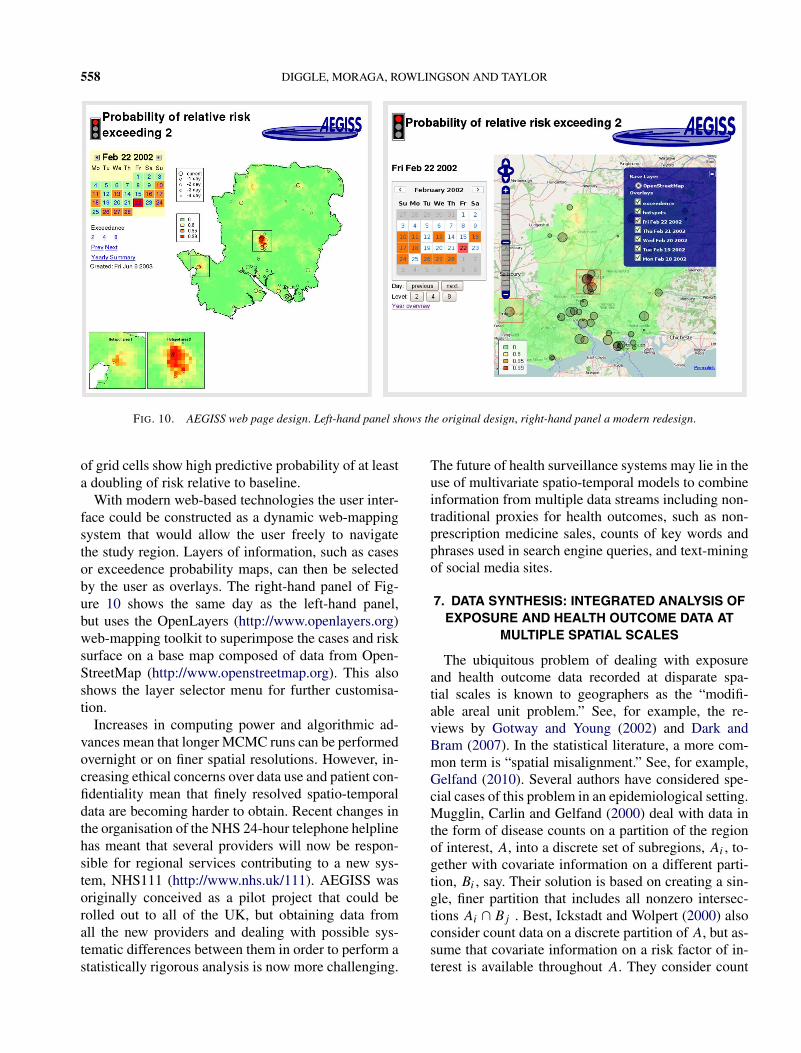
558 DIGGLE, MORAGA, ROWLINGSON AND TAYLOR
FIG. 10. AEGISS web page design. Left-hand panel shows the original design, right-hand panel a modern redesign.
of grid cells show high predictive probability of at leasta doubling of risk relative to baseline.
With modern web-based technologies the user inter-face could be constructed as a dynamic web-mappingsystem that would allow the user freely to navigatethe study region. Layers of information, such as casesor exceedence probability maps, can then be selectedby the user as overlays. The right-hand panel of Fig-ure 10 shows the same day as the left-hand panel,but uses the OpenLayers (http://www.openlayers.org)web-mapping toolkit to superimpose the cases and risksurface on a base map composed of data from Open-StreetMap (http://www.openstreetmap.org). This alsoshows the layer selector menu for further customisa-tion.
Increases in computing power and algorithmic ad-vances mean that longer MCMC runs can be performedovernight or on finer spatial resolutions. However, in-creasing ethical concerns over data use and patient con-fidentiality mean that finely resolved spatio-temporaldata are becoming harder to obtain. Recent changes inthe organisation of the NHS 24-hour telephone helplinehas meant that several providers will now be respon-sible for regional services contributing to a new sys-tem, NHS111 (http://www.nhs.uk/111). AEGISS wasoriginally conceived as a pilot project that could berolled out to all of the UK, but obtaining data fromall the new providers and dealing with possible sys-tematic differences between them in order to perform astatistically rigorous analysis is now more challenging.
The future of health surveillance systems may lie in theuse of multivariate spatio-temporal models to combineinformation from multiple data streams including non-traditional proxies for health outcomes, such as non-prescription medicine sales, counts of key words andphrases used in search engine queries, and text-miningof social media sites.
7. DATA SYNTHESIS: INTEGRATED ANALYSIS OFEXPOSURE AND HEALTH OUTCOME DATA AT
MULTIPLE SPATIAL SCALES
The ubiquitous problem of dealing with exposureand health outcome data recorded at disparate spa-tial scales is known to geographers as the “modifi-able areal unit problem.” See, for example, the re-views by Gotway and Young (2002) and Dark andBram (2007). In the statistical literature, a more com-mon term is “spatial misalignment.” See, for example,Gelfand (2010). Several authors have considered spe-cial cases of this problem in an epidemiological setting.Mugglin, Carlin and Gelfand (2000) deal with data inthe form of disease counts on a partition of the regionof interest, A, into a discrete set of subregions, Ai , to-gether with covariate information on a different parti-tion, Bi , say. Their solution is based on creating a sin-gle, finer partition that includes all nonzero intersec-tions Ai ∩ Bj . Best, Ickstadt and Wolpert (2000) alsoconsider count data on a discrete partition of A, but as-sume that covariate information on a risk factor of in-terest is available throughout A. They consider count
SPATIAL AND SPATIO-TEMPORAL LOG-GAUSSIAN COX PROCESSES 559
data to be derived from an underlying Cox processwhose intensity varies in a spatially continuous mannerthrough the combination of a covariate effect and a la-tent stochastic process modelled as a kernel-smoothedgamma random field. They then derive the distributionof the observed counts by spatial integration over theAi . Kelsall and Wakefield (2002) take a similar ap-proach, but using a log-Gaussian latent stochastic pro-cess rather than a gamma random field. The technicaland computational issues that arise when handling spa-tial integrals of stochastic processes can be simplifiedby using low-rank models, such as the class of Gaus-sian predictive process models proposed by Banerjee etal. (2008) and further developed by Finley et al. (2009).Gelfand (2012) gives a useful summary of this and re-lated work.
All of these approaches can be subsumed withina single modelling framework for multiple exposuresand disease risk by considering these as a set of spa-tially continuous processes, irrespective of the spatialresolution at which data elements are recorded. For ex-ample, a model for the spatial association between dis-ease risk, R(x), and m exposures Tk(x) :k = 1, . . . ,m
can be obtained by treating individual case-locations asan LGCP with intensity
R(x) = exp
{α +
p∑k=1
βkTk(x) + S(x)
},(29)
where S(x) denotes stochastic variation in risk thatis not captured by the p covariate processes Tk(x).The inferential algorithms associated with model (29)would then depend on the structure of the availabledata.
Suppose, for example, that health outcome data areavailable in the form of area-level counts, Yi : i =1, . . . , n, in subregions Ai , whilst exposure data are ob-tained as collections of unbiased estimates, Uik , of theTk(x) at corresponding locations xik : i = 1, . . . ,mk .Suppose further that the Uik are conditionally indepen-dent, with Uik|Tk(·) ∼ N(Tk(xik), τ
2k ), the processes
Tk(·) are jointly Gaussian and the process S(·) is alsoGaussian and independent of the Tk(·). A possible in-ferential goal is to evaluate the predictive distributionof the risk surface R(·) given the data Yi : i = 1, . . . ,m
and Uik : i = 1, . . . ,mk;k = 1, . . . , p. In an obviousshorthand, and temporarily ignoring the issue of pa-rameter estimation, the required predictive distributionis [S,T |U,Y ]. The joint distribution of S, T , U and Y
factorises as
[S,T ,U,Y ] = [S][T ][U |T ][Y |S,T ],(30)
where [S] and [T ] are multivariate Gaussian densities,[U |T ] is a product of univariate Gaussian densities,and [Y |S,T ] is a product of Poisson probability dis-tributions with means
μi =∫Ai
R(x) dx.
Sampling from the required predictive distributionscan then proceed using a suitable MCMC algorithm.For Bayesian parameter estimation, we would augment(30) by a suitable joint prior for the model parametersbefore designing the MCMC algorithm.
A specific example of data synthesis concerns anongoing leptospirosis cohort study in a poor commu-nity within the city of Salvador, Brazil. Leptospirosis isconsidered to be the most widespread of the zoonoticdiseases. This is due to the large number of peopleworldwide, but especially in poor communities, wholive in close proximity to wild and domestic mam-mals that serve as reservoirs of infection and shed theagent in their urine. The major mode of transmission iscontact with contaminated water or soil (Levett, 2001;Bharti et al., 2003; McBride et al., 2005). In the major-ity of cases infection leads to an asymptomatic or mild,self-limiting febrile illness. However, severe cases canlead to potentially fatal acute renal failure and pul-monary haemorrhage syndrome. Leptospirosis is tradi-tionally associated with rural-based subsistence farm-ing communities, but rapid urbanization and wideningsocial inequality have led to the dramatic growth of ur-ban slums, where the lack of basic sanitation favoursrat-borne transmission (Ko et al., 1999; Johnson et al.,2004).
The goals of the cohort study are to investigate thecombined effects of social and physical environmen-tal factors on disease risk, and to map the unexplainedspatio-temporal variation in incidence. In the study,approximately 1700 subjects i = 1, . . . , n at residen-tial locations xi provide blood-samples on recruitmentand at subsequent times tij approximately 6, 12, 18and 24 months later. At each post-recruitment visit,sero-conversion is defined as a change from zero topositive, or at least a fourfold increase in concentra-tion. The resulting data consist of binary responses,Yij = 0/1 : j = 1,2,3,4 (sero-conversion no/yes), to-gether with a mix of time-constant and time-varyingrisk-factors, rij .
A conventional analysis might treat the data fromeach subject as a time-sequence of binary responseswith associated explanatory variables. Widely used
560 DIGGLE, MORAGA, ROWLINGSON AND TAYLOR
methods for data of this kind include generalised es-timating equations (Liang and Zeger, 1986) and gen-eralised linear mixed models (Breslow and Clayton,1993). An analysis more in keeping with the philos-ophy of the current paper would proceed as follows.
Let ai and bi(t) denote time-constant and time-varying explanatory variables associated with subject i,and tij the times at which blood samples are taken, set-ting ti0 = 0 for all i. Note that explanatory variablescan be of two distinct kinds: characteristics of an indi-vidual subject, for example, their age; and character-istics of a subject’s place of residence, for example,its proximity to an open-sewer. In principle, the lat-ter can be indexed by a spatially continuous location,hence, ai = A(xi) and bi(t) = B(xi, t). A responseYij = 1 indicates that at least one infection event hasoccurred in the time-interval (ti,j−1, tij ). A model foreach subject’s risk of infection then requires the spec-ification of a set of person-specific hazard functions,�i(t). A model that allows for unmeasured risk factorswould be a set of LGCPs, one for each subject, withrespective stochastic intensities,
�i(t) = exp{a′iα + bi(tij )
′β + Ui + S(xi, t)},(31)
where the Ui are mutually independent N(0, ν2) andS(x, t) is a spatio-temporally continuous Gaussian pro-cess. It follows that
P{Yit = 1|�i(·)}
(32)
= 1 − exp{−
∫ tij
ti,j−1
�i(u)du
}.
In practice, values of a(x) and b(x, t) may only be ob-served incompletely, either at a finite number of lo-cations or as small-area averages. For notational con-venience, we consider only a single, incompletely ob-served spatio-temporal covariate whose measured val-ues, bk :k = 1, . . . ,m, we model as
bk = B(xk, tk) + Zk,(33)
where B(x, t) is a spatio-temporal Gaussian processand the Zk are mutually independent N(0, τ 2) mea-surement errors. Then, (31) becomes
�i(t) = exp{B(xi, tij )
′β + Ui + S(xi, t)}.(34)
Inference for the model defined by (32), (33) and (34),based on data {yij : j = 1, . . . ,4; i = 1, . . . , n} and b ={bk :k = 1, . . . ,m}, would require further developmentof MCMC algorithms of the kind described in Sec-tion 4.
8. DISCUSSION
In this paper we have argued that the LGCP pro-vides a useful class of models, not only for point pro-cess data but also for any problem involving predictionof an incompletely observed spatial or spatio-temporalprocess, irrespective of data format. Developments instatistical computation have made the combination oflikelihood-based, classical or Bayesian parameter es-timation and probabilistic prediction feasible for rela-tively large data sets, including real-time updating ofspatio-temporal predictions.
In each of our applications, the focus has been onprediction of the spatial or spatio-temporal variation ina response surface, rather than on estimation of modelparameters. In problems of this kind, where parame-ters are not of direct interest but rather are a means toan end, Bayesian prediction in conjunction with diffusepriors is an attractive strategy, as its predictions natu-rally accommodate the effect of parameter uncertainty.Model-based predictions are essentially nonparametricsmoothers, but embedded within a probabilistic frame-work. This encourages the user to present results in away that emphasises, rather than hides, their inherentimprecision.
In many public health settings, identifying where andwhen a particular phenomenon, such as disease inci-dence, is likely to have exceeded an agreed interven-tion threshold is more useful than quoting either a pointestimate and its standard error or the statistical signifi-cance of departure from a benchmark.
The log-linear formulation is convenient because ofthe tractable moment properties of the log-Gaussiandistribution. It also gives the model a natural interpre-tation as a multiplicative decomposition of the overallintensity into deterministic and stochastic components.However, it can lead to very highly skewed marginaldistributions, with large patches of near-zero intensityinterspersed with sharp peaks. Within the Monte Carloinferential framework, there is no reason why other,less severe transformations from R to R
+ should notbe used.
Two areas of current methodological research arethe formulation of models and methods for princi-pled analysis of multiple data streams that include dataof variable quality from nontraditional sources, andthe further development of robust computational algo-rithms that can deliver reliable inferences for problemsof ever-increasing complexity.
Our general approach reflects a continuing trend inapplied statistics since the 1980s. The explosion in
SPATIAL AND SPATIO-TEMPORAL LOG-GAUSSIAN COX PROCESSES 561
the development of computationally intensive methodsand associated complex stochastic models has encour-aged a move away from a methods-based classifica-tion of the statistics discipline and towards a multi-disciplinary, problem-based focus in which statisticalmethod (singular) is thoroughly embedded within sci-entific method.
ACKNOWLEDGEMENTS
We thank the Department of Environmental andCancer Epidemiology in the National Center For Epi-demiology (Spain) for providing aggregated data fromthe Castile-La Mancha region for permission to use theSpanish lung cancer data.
The leptospirosis study described in Section 7 isfunded by a USA National Science Foundation grant,with Principal Investigator Professor Albert Ko (YaleUniversity School of Public Health). This work wassupported by the UK Medical Research Council (Grantnumber G0902153).
SUPPLEMENTARY MATERIAL
Supplementary materials for “Spatial and spatio-temporal log-Gaussian Cox processes: Extendingthe geostatistical paradigm” (DOI: 10.1214/13-STS441SUPP; .pdf). This material contains mixing,convergence and inferential diagnostics for all of theexamples in the main article and is also available fromhttp://www.lancs.ac.uk/staff/taylorb1/statsciappendix.pdf.
REFERENCES
ANDRIEU, C. and THOMS, J. (2008). A tutorial on adaptiveMCMC. Stat. Comput. 18 343–373. MR2461882
BADDELEY, A. J., MØLLER, J. and WAAGEPETERSEN, R.(2000). Non- and semi-parametric estimation of interactionin inhomogeneous point patterns. Stat. Neerl. 54 329–350.MR1804002
BANERJEE, S., GELFAND, A. E., FINLEY, A. O. and SANG, H.(2008). Gaussian predictive process models for large spatialdata sets. J. R. Stat. Soc. Ser. B Stat. Methodol. 70 825–848.MR2523906
BARTLETT, M. S. (1964). The spectral analysis of two-dimensional point processes. Biometrika 51 299–311.MR0175254
BARTLETT, M. S. (1975). The Statistical Analysis of Spatial Pat-tern. Chapman & Hall, London. MR0402886
BERMAN, M. and DIGGLE, P. (1989). Estimating weighted inte-grals of the second-order intensity of a spatial point process.J. R. Stat. Soc. Ser. B Stat. Methodol. 51 81–92. MR0984995
BESAG, J., YORK, J. and MOLLIÉ, A. (1991). Bayesian imagerestoration, with two applications in spatial statistics. Ann. Inst.Statist. Math. 43 1–59. MR1105822
BEST, N. G., ICKSTADT, K. and WOLPERT, R. L. (2000). Spa-tial Poisson regression for health and exposure data measuredat disparate resolutions. J. Amer. Statist. Assoc. 95 1076–1088.MR1821716
BHARTI, A. R., NALLY, J. E., RICALDI, J. N.,MATTHIAS, M. A., DIAZ, M. M., LOVETT, M. A., LEV-ETT, P. N., GILMAN, R. H., WILLIG, M. R., GOTUZZO, E.and VINETZ, J. M. (2003). Leptospirosis: A zoonotic diseaseof global importance. Lancet. Infect. Dis. 3 757–771.
BRESLOW, N. E. and CLAYTON, D. G. (1993). Approximate in-ference in generalized linear mixed models. J. Amer. Statist. As-soc. 88 9–25.
BRIX, A. and DIGGLE, P. J. (2001). Spatiotemporal predictionfor log-Gaussian Cox processes. J. R. Stat. Soc. Ser. B Stat.Methodol. 63 823–841. MR1872069
BRIX, A. and DIGGLE, P. J. (2003). Corrigendum: Spatio-temporal prediction for log-Gaussian Cox processes. J. R. Stat.Soc. Ser. B Stat. Methodol. 65 946.
BROWN, P. E., KÅRESEN, K. F., ROBERTS, G. O. and TONEL-LATO, S. (2000). Blur-generated non-separable space–timemodels. J. R. Stat. Soc. Ser. B Stat. Methodol. 62 847–860.MR1796297
COOPER, D. and CHINEMANA, F. (2004). NHS direct deriveddata: An exciting new opportunity or an epidemiologicalheadache? J. Public Health (Oxf.) 26 158–160.
COOPER, D. L., SMITH, G. E., O’BRIEN, S. J., HOL-LYOAK, V. A. and BAKER, M. (2003). What can analysis ofcalls to NHS direct tell us about the epidemiology of gastroin-testinal infections in the community? J. Infect. 46 101–105.
COX, D. R. (1955). Some statistical methods connected with seriesof events. J. R. Stat. Soc. Ser. B Stat. Methodol. 17 129–157;discussion, 157–164. MR0092301
CRESSIE, N. A. C. (1991). Statistics for Spatial Data. Wiley, NewYork. MR1127423
CRESSIE, N. and HUANG, H.-C. (1999). Classes of nonsepara-ble, spatio-temporal stationary covariance functions. J. Amer.Statist. Assoc. 94 1330–1340. MR1731494
DARK, S. J. and BRAM, D. (2007). The modifiable areal unit prob-lem (MAUP) in physical geography. Progress in Physical Ge-ography 31 471–479.
DIGGLE, P. J. and RIBEIRO, P. J. JR. (2007). Model-Based Geo-statistics. Springer, New York. MR2293378
DIGGLE, P., ROWLINGSON, B. and SU, T.-L. (2005). Point pro-cess methodology for on-line spatio-temporal disease surveil-lance. Environmetrics 16 423–434. MR2147534
DIGGLE, P. J., ZHENG, P. and DURR, P. (2005). Non-parametricestimation of spatial segregation in a multivariate point process.Applied Statistics 54 645–658.
DIGGLE, P. J., KNORR-HELD, L., ROWLINGSON, B., SU, T.,HAWTIN, P. and BRYANT, T. (2003). Towards on-line spatialsurveillance. In Monitoring the Health of Populations: Statis-tical Methods for Public Health Surveillance (R. Brookmeyerand D. Stroup, eds.). Oxford Univ. Press, Oxford.
DIGGLE, P. J., MORAGA, P., ROWLINGSON, B. and TAY-LOR, B. M. (2013). Supplement to “Spatial and spatio-temporal log-Gaussian Cox processes: Extending the geostatis-tical paradigm.” DOI:10.1214/13-STS441SUPP.
562 DIGGLE, MORAGA, ROWLINGSON AND TAYLOR
DONNELLY, C. A., WOODROFFE, R., COX, D. R.,BOURNE, F. J., CHEESMAN, C. L., CLIFTON-HADLEY, R. S.,WEI, G., GETTINBY, G., GILKS, P., JENKINS, H., JOHN-STON, W. T., LE FEVRE, A. M., MCINERY, J. P. andMORRISON, W. I. (2006). Positive and negative effects ofwidespread badger culling on tuberculosis in cattle. Nature 485843–846.
FINLEY, A. O., SANG, H., BANERJEE, S. and GELFAND, A. E.(2009). Improving the performance of predictive process mod-eling for large datasets. Comput. Statist. Data Anal. 53 2873–2884. MR2667597
FRIGO, M. and JOHNSON, S. G. (2011). FFTW fastest Fouriertransform in the west. Available at http://www.fftw.org/.
GAMERMAN, D. (2010). Dynamic spatial models including spatialtime series. In Handbook of Spatial Statistics (A. E. Gelfand,P. J. Diggle, M. Fuentes and P. Guttorp, eds.) 437–448. CRCPress, Boca Raton, FL. MR2730959
GAMERMAN, D. and LOPES, H. F. (2006). Markov Chain MonteCarlo: Stochastic Simulation for Bayesian Inference, 2nd ed.Chapman & Hall/CRC, Boca Raton, FL. MR2260716
GELFAND, A. E. (2010). Misaligned spatial data: The changeof support problem. In Handbook of Spatial Statistics(A. E. Gelfand, P. J. Diggle, M. Fuentes and P. Guttorp, eds.)517–539. CRC Press, Boca Raton, FL. MR2730964
GELFAND, A. E. (2012). Hierarchical modelling for spatial dataproblems. Spatial Statistics 1 30–39.
GELFAND, A. E., DIGGLE, P. J., FUENTES, M. and GUTTORP, P.,eds. (2010). Handbook of Spatial Statistics. CRC Press, BocaRaton, FL. MR2761512
GEMAN, S. and GEMAN, D. (1984). Stochastic relaxation, Gibbsdistributions, and the Bayesian restoration of images. IEEETrans. Pattern. Anal. Mach. Intell. 6 721–741.
GERRARD, D. J. (1969). Competition Quotient: A New Measureof the Competition Affecting Individual Forest Trees. ResearchBulletin 20. Agricultural Experiment Station, Michigan StateUniv., East Lansing, MI.
GEYER, C. (1999). Likelihood inference for spatial point pro-cesses: Likelihood and computation. In Stochastic Geometry(Toulouse, 1996), (O. E. Barndorff-Nielsen, W. S. Kendall andM. N. M. van Lieshout, eds.). Monogr. Statist. Appl. Probab. 8079–140. Chapman & Hall/CRC, Boca Raton, FL. MR1673118
GILKS, W., RICHARDSON, S. and SPIEGELHALTER, D. (1995).Markov Chain Monte Carlo in Practice. Chapman & Hall, Lon-don.
GIROLAMI, M. and CALDERHEAD, B. (2011). Riemann manifoldLangevin and Hamiltonian Monte Carlo methods. J. R. Stat.Soc. Ser. B Stat. Methodol. 73 123–214. MR2814492
GNEITING, T. (2002). Nonseparable, stationary covariance func-tions for space–time data. J. Amer. Statist. Assoc. 97 590–600.MR1941475
GNEITING, T. and GUTTORP, P. (2010a). Continuous parame-ter stochastic process theory. In Handbook of Spatial Statistics(A. E. Gelfand, P. J. Diggle, M. Fuentes and P. Guttorp, eds.)17–28. CRC Press, Boca Raton, FL. MR2730952
GNEITING, T. and GUTTORP, P. (2010b). Continuous parameterspatio-temporal processes. In Handbook of Spatial Statistics(A. E. Gelfand, P. J. Diggle, M. Fuentes and P. Guttorp, eds.)427–436. CRC Press, Boca Raton, FL. MR2730958
GOTWAY, C. A. and YOUNG, L. J. (2002). Combining in-compatible spatial data. J. Amer. Statist. Assoc. 97 632–648.MR1951636
GREENLAND, S. and MORGENSTERN, H. (1990). Ecological bias,confounding and effect modification. International Journal ofEpidemiology 18 269–274.
HARAN, M. and TIERNEY, L. (2012). On automating Markovchain Monte Carlo for a class of spatial models. Available athttp://arxiv.org/abs/1205.0499.
HASTINGS, W. K. (1970). Monte Carlo sampling methods usingMarkov chains and their applications. Biometrika 57 97–109.
JOHNSON, M. A., SMITH, H., JOSEPH, P., GILMAN, R. H.,BAUTISTA, C. T., CAMPOS, K. J., CESPEDES, M.,KLATSKY, P., VIDAL, C., TERRY, H., CALDERON, M. M.,CORAL, C., CABRERA, L., PARMAR, P. S. and VINETZ, J. M.(2004). Environmental exposure and leptospirosis, Peru.Emerging Infectious Diseases 10 1016–1022.
KELSALL, J. and WAKEFIELD, J. (2002). Modeling spatial varia-tion in disease risk: A geostatistical approach. J. Amer. Statist.Assoc. 97 692–701. MR1941405
KO, A. I., REIS, M. G., DOURADO, C. M. R., JOHNSON, W. D.JR. and RILEY, L. W. (1999). Urban epidemic of severeleptospirosis in Brazil. Salvador Leptospirosis Study Group.Lancet 354 820–825.
LEVETT, P. N. (2001). Leptospirosis. Clininical Microbiology Re-views 14 296–326.
LI, Y., BROWN, P. E., GESINK, D. C. and RUE, H. (2012). LogGaussian Cox processes and spatially aggregated disease inci-dence data. Stat. Methods Med. Res. 21 479–507.
LIANG, K. Y. and ZEGER, S. L. (1986). Longitudinal data anal-ysis using generalized linear models. Biometrika 73 13–22.MR0836430
LINDGREN, F., RUE, H. and LINDSTRÖM, J. (2011). An explicitlink between Gaussian fields and Gaussian Markov randomfields: The stochastic partial differential equation approach. J. R.Stat. Soc. Ser. B Stat. Methodol. 73 423–498. MR2853727
LÓPEZ-ABENTE, G., RAMIS, R., POLLÁN, M., ARAGONÉS, N.,PÉREZ-GÓMEZ, B., GÓMEZ-BARROSO, D., CAR-RASCO, J. M., LOPE, V., GARCÍA-PÉREZ, J., BOLDO, E.and GARCÍA-MENDIZÁBAL, M. J. (2006). ATLAS municipalde mortalidad por cáncer en España, 1989–1998. Instituto deSalud Carlos III, Madrid.
MA, C. (2003). Families of spatio-temporal stationary covariancemodels. J. Statist. Plann. Inference 116 489–501. MR2000096
MA, C. (2008). Recent developments on the construction of spatio-temporal covariance models. Stoch. Environ. Res. Risk Assess.22 39–47. MR2418410
MARK, A. L. and SHEPHERD, D. H. (2004). NHS Direct: Manag-ing demand for primary care? International Journal of HealthPlanning and Management 19 79–91.
MATÉRN, B. (1960). Spatial Variation. Meddelanden fran StatensSkogsforskningsinstitut, Stockholm. Band 49, number 5.MR0169346
MCBRIDE, A. J., ATHANAZIO, D. A., REIS, M. G. and KO, A. I.(2005). Leptospirosis. Current Opinions in Infectious Diseases18 376–386.
METROPOLIS, N., ROSENBLUTH, A. W., ROSENBLUTH, M. N.,TELLER, A. H. and TELLER, E. (1953). Equation of state cal-culations by fast computing machines. The Journal of ChemicalPhysics 21 1087–1092.
MØLLER, J., SYVERSVEEN, A. R. and WAAGEPETERSEN, R. P.(1998). Log Gaussian Cox processes. Scand. J. Stat. 25 451–482. MR1650019
SPATIAL AND SPATIO-TEMPORAL LOG-GAUSSIAN COX PROCESSES 563
MUGGLIN, A. S., CARLIN, B. P. and GELFAND, A. E. (2000).Fully model-based approaches for spatially misaligned data.J. Amer. Statist. Assoc. 95 877–887.
PIANTADOSI, S., BYAR, D. P. and GREEN, S. B. (1988). The eco-logical fallacy. Am. J. Epidemiol. 127 893–904.
R CORE TEAM. (2013). R: A Language and Environment for Sta-tistical Computing. Vienna, Austria.
RIPLEY, B. D. (1976). The second-order analysis of stationarypoint processes. J. Appl. Probab. 13 255–266. MR0402918
RIPLEY, B. D. (1977). Modelling spatial patterns. J. R. Stat. Soc.Ser. B Stat. Methodol. 39 172–212. MR0488279
ROBERTS, G. O. and ROSENTHAL, J. S. (2001). Optimal scal-ing for various Metropolis–Hastings algorithms. Statist. Sci. 16351–367. MR1888450
ROBERTS, G. O. and ROSENTHAL, J. S. (2007). Coupling andergodicity of adaptive Markov chain Monte Carlo algorithms.J. Appl. Probab. 44 458–475. MR2340211
ROBERTS, G. O. and TWEEDIE, R. L. (1996). Exponential con-vergence of Langevin distributions and their discrete approxi-mations. Bernoulli 2 341–363. MR1440273
RODRIGUES, A. and DIGGLE, P. J. (2010). A class of convolution-based models for spatio-temporal processes with non-separablecovariance structure. Scand. J. Stat. 37 553–567. MR2779636
RUE, H. and HELD, L. (2005). Gaussian Markov Random Fields:Theory and Applications. Monographs on Statistics and Ap-plied Probability 104. Chapman & Hall/CRC, Boca Raton, FL.MR2130347
RUE, H., MARTINO, S. and CHOPIN, N. (2009). ApproximateBayesian inference for latent Gaussian models by using inte-grated nested Laplace approximations. J. R. Stat. Soc. Ser. BStat. Methodol. 71 319–392. MR2649602
SILVERMAN, B. W. (1986). Density Estimation for Statistics andData Analysis. Chapman & Hall, London. MR0848134
SPIEGELHALTER, D. J., THOMAS, A. and BEST, N. G. (1999).WinBUGS Version 1.2 User Manual.
TAYLOR, B. M. and DIGGLE, P. J. (2013a). INLA or MCMC?A tutorial and comparative evaluation for spatial prediction inlog-Gaussian Cox processes. J. Stat. Comput. Simul. To appear.Preprint available at http://arxiv.org/abs/1202.1738.
TAYLOR, B. M. and DIGGLE, P. J. (2013b). Corrigendum: Spa-tiotemporal prediction for log-Gaussian Cox processes. J. R.Stat. Soc. Ser. B Stat. Methodol. 75 601–602. MR3065481
TAYLOR, B. M., DAVIES, T. M., ROWLINGSON, B. S. and DIG-GLE, P. J. (2013). lgcp: Inference with spatial and spatio-temporal log-Gaussian Cox processes in R. Journal of Statis-tical Software 52 Issue 4.
WALL, M. M. (2004). A close look at the spatial structure impliedby the CAR and SAR models. J. Statist. Plann. Inference 121311–324. MR2038824
WOOD, A. T. A. and CHAN, G. (1994). Simulation of stationaryGaussian processes in [0,1]d . J. Comput. Graph. Statist. 3 409–432. MR1323050
WOODROFFE, R., DONNELLY, C. A., JOHNSTON, W. T.,BOURNE, F. J., CHEESMAN, C. L., CLIFTON-HADLEY, R. S.,COX, D. R., GETTINBY, G., HEWINSON, R. G.,LE FEVRE, A. M., MCINERY, J. P. and MORRISON, W. I.(2005). Spatial association of Mycobacterium bovis infection incattle and badgers Meles meles. Journal of Applied Ecology 42852–862.
ZHANG, H. (2004). Inconsistent estimation and asymptoticallyequal interpolations in model-based geostatistics. J. Amer.Statist. Assoc. 99 250–261. MR2054303