spatial and temporal modulation of heat source using light
TRANSCRIPT

Scholars' Mine Scholars' Mine
Masters Theses Student Theses and Dissertations
Spring 2015
Spatial and temporal modulation of heat source using light Spatial and temporal modulation of heat source using light
modulator for advanced thermography modulator for advanced thermography
Arvindvivek Ravichandran
Follow this and additional works at: https://scholarsmine.mst.edu/masters_theses
Part of the Mechanical Engineering Commons
Department: Department:
Recommended Citation Recommended Citation Ravichandran, Arvindvivek, "Spatial and temporal modulation of heat source using light modulator for advanced thermography" (2015). Masters Theses. 7411. https://scholarsmine.mst.edu/masters_theses/7411
This thesis is brought to you by Scholars' Mine, a service of the Missouri S&T Library and Learning Resources. This work is protected by U. S. Copyright Law. Unauthorized use including reproduction for redistribution requires the permission of the copyright holder. For more information, please contact [email protected].

SPATIAL AND TEMPORAL MODULATION OF HEAT SOURCE USING LIGHT
MODULATOR FOR ADVANCED THERMOGRAPHY
by
ARVINDVIVEK RAVICHANDRAN
A THESIS
Presented to the Faculty of the Graduate School of the
MISSOURI UNIVERSITY OF SCIENCE AND TECHNOLOGY
In Partial Fulfillment of the Requirements for the Degree
MASTER OF SCIENCE IN MECHANICAL ENGINEERING
2015
Approved by
Edward Kinzel, Advisor
Xiaodong Yang
Hai-Lung Tsai

2015
Arvindvivek Ravichandran
All Rights Reserved

iii
ABSTRACT
Thermography is a Non-Destructive Testing (NDT) method that has found
increasing use in industry and research. It has the advantages of being non-contact and be
able to interrogate a large surface simultaneously. Active thermography using flash lamps
as heat source has been demonstrated for identifying blind holes and delamination in
composites. Despite these advancements, active thermographic approach fails to defects
like cracks. Under uniform illumination heat flow is predominantly 1D and can easily
circumvent a narrow feature. This can be overcome by using a focused light/laser source
onto the surface to impose a 3D heat flux. The disadvantage is that thermography is now
a point-by-point proposition, because the focused heat source interrogates only a
localized region. This work investigates the use of a Digital Micro mirror Device (DMD)
to modulate the illumination both spatially and temporally. This allows multiple point or
line sources to simultaneously illuminate a surface at independent frequencies. The use of
frequency modulation maps the results to phase space, which permits data to be extracted
even when the thermal camera is not precisely calibrated, in combination with the low
cost of the DMDs. This thesis describes the construction of the experiment, the theory
behind the technique, demonstrates the setup for conventional thermographic methods
(pulse/flash and lock-in) before demonstrating the ability to demodulate a locally varying
heat flux. The thesis also presents the use of the setup for rudimentary system
identification which is similar to Photo Thermal Radiometry, and extends the use of the
setup to distinguish films from the underlying substrate, in addition to crack detection.
Numeric simulations in ANSYS used to guide this work are also presented along with
suggestions for future improvement of the setup and scale-up to larger systems.
iv
ACKNOWLEDGMENTS
I would like to extend my sincere thanks to my advisor Dr Ed Kinzel who has
been motivating me during the course of this research. We had numerous thoughtful and
inspiring discussions on different topics during my stay in Thermal Radiation Laboratory,
which are extremely valuable.
I would like to extend my sincere appreciation to my committee members Dr
Xiadong Yang and Dr Tsai for their immense advice during the course of the Research.
Special thanks to Dr Tsai for letting me use the facilities of his lab and his valuable
advice during the Laser Aided Manufacturing coursework.
My sincere thanks to Dr Landers and the Department of Mechanical Engineering
for the financial support towards my tuition.
I would like to thank my fellow lab members Harsh, Luo, Jacob and Chuang for
their help and thoughtful conversation during my stay.
Special thanks to my parents for their patience and constant motivation. Without
them I wouldn’t have made it possible.
Last, but not the least. I would like to thank Hannah, Rose and John who would
visit the lab to spread their joy and make others forget their worries by their contagious
smile.
v
TABLE OF CONTENTS
ABSTRACT .................................................................................................................. iii
ACKNOWLEDGMENTS ............................................................................................. iv
LIST OF ILLUSTRATIONS ........................................................................................ vii
LIST OF TABLES ..........................................................................................................x
NOMENCLATURE ...................................................................................................... xi
SECTION
1. INTRODUCTION ...................................................................................................1
1.1. NON DESTRUCTIVE TESTING ....................................................................2
1.2. NDT THERMOGRAPHY……………………………………………………...2
1.1.1. Pulsed Thermography ............................................................................4
1.1.2. Lock-in Thermography ......................................................................... .7
1.3. SPATIAL TEMPORAL MODULATION TECHNIQUE……………………..8
1.4. MOTIVATION……………………………………………………………….10
1.5. THESIS OVERVIEW………………………………………………………...11
2. DMD DEVICE- ITS ARCHITECHTURE AND CAPABILITIES ................ ……12
2.1. DMD DEVICE .............................................................................................. 12
2.2. EXPERIMENTAL SETUP ............................................................................ 14
2.3 CAPABILITIES OF THE DEVICE ................................................................ 15
2.3.1. Pulse Thermography ............................................................................ 16
2.3.2. Lock-in Thermography ........................................................................ 17
2.3.3. Spatial and Temporal Modulated Thermography .................................. 18
2.4 LINEAR CO-ORDINATE TRANSFORMATION……………………….......20
3. NUMERICAL ANALYSIS ................................................................................. ..23
3.1. GOVERNING EQUATION ........................................................................... 23
3.2. BOUNDARY CONDITION .......................................................................... 25
3.3. FINITE ELEMENT MODELING .................................................................. 25
3.3.1. Geometric Modeling ............................................................................ 25
3.3.2. Meshing ............................................................................................... 26
3.3.3. Solution and Post Processing ................................................................ 27

vi
4. RESULTS ............................................................................................................. 29
4.1. NUMERICAL RESULTS .............................................................................. 29
4.1.1. Pulse Thermography ............................................................................ 30
4.1.2. Lock-in Thermography ........................................................................ 31
4.1.3.Spatial and Temporal Modulation Thermography .................................. 32
4.2. EXPERIMENTAL RESULTS ........................................................................ 33
4.2.1. Pulse Thermography ............................................................................ 33
4.2.2. Lock-in Thermography ........................................................................ 34
4.2.3. Crack Identification .............................................................................. 35
4.2.4. Multiple Spatial and Temporal Modulation .......................................... 36
4.2.5. Thermal Property Estimation for System Identification ....................... 38
5. CONCLUSION AND FUTURE WORK……………………………………………..41
5.1. CONCLUSION………………………………………………………………...41
5.2. FUTURE WORK………………………………………………………............41
5.2.1. Direction-1……………………………………………………………..42
5.2.2. Direction-2…………………………………………………………..…42
5.2.3. Direction-3……………………………………………………………..42
APPENDIX. .................................................................................................................. 45
BIBLIOGRAPHY ......................................................................................................... 56
VITA ............................................................................................................................ 60
vii
LIST OF ILLUSTRATIONS
Figure Page
1.1 Typical Thermography Set up of the sample and the IR Camera…………………...4
1.2 Experimental Set-Up of the Pulse Thermography………………………………......4
1.3 2-D Side View of Sample (a) Without Defect (b) With Defect with Pulse
Thermography……………………………………………………………………….6
1.4 Conventional experimental set up of the Lock-in thermography……………………6
1.5 3-D Block Diagram representing the simplified experimental set-up………………7
1.6 The laser beam raster and pulse over the surface as per the desired frequency….....9
2.1 Micro mirror architecture present in DMD……………………………………….....10
2.2 SEM image of the Micro mirror Array……………………………………………...12
2.3 Experimental set up inside the shielded enclosure…………………………….........14
2.4 Experimental setup where laser is collimated over the DMD array…………………15
2.5 Sample is pulsed at different diameter by the DMD Device………………………...15
2.6 Sample is pulsed at different frequency and profile by DMD Device………………17
2.7 Sample is probed by scanning laser beam by DMD Device………………………...18
2.8 Temporal Modulation by DMD Device by different frequencies…………………...19
2.9 Linear Co-ordinate transformation mapping from the computer to the sample…….19
2.10 Mapping of co-ordinates between different planes…………………………………20
3.1 Dimension of the sample as made in Design Modeler of Ansys Workbench 14……21
3.2 Named Selection in the geometric modeling to specify Thermal load………………25
3.3 Tetrahedron Mesh with fine refinement on the area of interest……………………...26
viii
3.4. Mesh Setting………………………………………………………………………..26
4.1. Pulse Thermography on wide defect……………………………………………….30
4.2. Pulse Thermography on narrow defect……………………………………………..30
4.3. Lock-in Thermography on wide defect……………………………………………..31
4.4. Lock-in Thermography on narrow defect…………………………………………..31
4.5. Spatially modulated Pulse Thermography…………………………………………..32
4.6. Spatially and Temporally modulated Lock-in Thermography …………………..…32
4.7. 15 sec Pulse Thermography………………………………………………………....33
4.8. Amplitude and Phase image of the defective ABS sample………………………….34
4.9. FFT plot and the location of defects as shown in Figure.4.8………………………..34
4.10. Amplitude and Phase map of spatially and temporally modulated heat source.......35
4.11. Amplitude and Phase segment transverse to the crack ……………………………36
4.12. Segment of Raw signal from the DRS camera and the corresponding color image.37
4.13. FFT plot of each line……………………………………………………………….37
4.14. Amplitude and Phase plot corresponding to 1Hz and 2Hz………………………..38
4.15. Amplitude and Phase plot corresponding of 600mHz shining at FR-4 surface …...39
4.16. Amplitude and Phase plot on FR-4 (on Left) along with FFT plot (on Right)…….39
4.17. Amplitude and Phase plot corresponding to 600mHz shining at copper cladding
surface……………………………………………………………………………...40
4.18. Amplitude and Phase plot on Copper cladding (on Left) along with FFT plot (on
Right)………………………………………………………………………………40
5.1. Parametric Optimization and Control theory…………………………………….....42

ix
5.2. Feedback based Closed Loop Optimal Control Problem……………………….......42
5.3 Structured light 3D scanner scanning a car seat to generate 3-D profile [24]……....43

x
LIST OF TABLES
Table Page
3.1. Solution Setting for Pulse Thermography…………………………………………..35
3.2. Solution Setting for Lock-in Thermography………………………………………..36
4.1. Properties of FR-4 used in the simulation…………………………………………..37
xi
NOMENCLATURE
Symbol Description
Q Heat Flux in W/m2
T Temperature in ˚C
cp Specific Heat in J/kg. K
φ Phase in Radian
ρ Density in kg/m3
ε Radiation Emissivity
ω Angular Frequency in rad/s
f Frequency in Hz
z Thermal Penetration Depth
k Thermal Conductivity in W/mk
Thermal Diffusivity in m2/s
t Time in Seconds

1. INTRODUCTION
In today’s manufacturing Industry the goal is to march towards excellence with
zero tolerance in defects. The goal seems unrealistic due to the volume of products that
are manufactured for the ever increase in the consumers. To touch the unrealistic goal,
companies started implementing systematic quality improvement tools like sig sigma,
lean, kaizen etc. In order to measure their progress, they rely on statistical methods which
compute the estimate of quality with certain confidence intervals by random sampling of
lot. The computed value is still an estimate and is not exact. Hence, the future is to ensure
the quality of all the products that are manufactured by nondestructive methods using
autonomous systems. This is enabled with the advanced tools developed under the
science of Non-Destructive Testing [NDT]. NDT is not only important for ensuring the
quality of the products during manufacturing process but also for verifying the quality
during service hours. It is highly important in aerospace industry where the quality of the
aircraft should be monitored before every flight in order to make sure there is zero
percent failure [1, 2]
1.1 NON-DESTRUCTIVE TESTING
Non-Destructive Testing is a self-explanatory word describing the ability to
identify discontinuities or defects without dissecting apart the component under study.
This science of Non-Destructive Testing is very old. The early chronological events are
described in the handbook of nondestructive evaluation[3].
NDT has several advantages compared to its peers. Some of the key features
are (i) NDT is highly useful because of its capability to be deployed at larger scale. NDT
can inspect the defects in the entire batch under production rather than testing random
samples in batch. This brings more confidence in the quality of the product. (ii) The
sample under study can be inspected even when it is performing its functionality (iii) The
testing is simple and cost effective in most of the cases. (iv) The sample is not damaged
or influenced under by the NDT when chosen aptly.

2
It has a wide variety of applications and is applied in diverse industries like
aviation[1, 2, 4, 5], semiconductor[6-8] , manufacturing [9, 10], military[11, 12] ,
automotive [9, 13, 14]etc.
Out of the several applications, the most common defects are used to evaluate the
structural defects like cracks, delamination, blow holes or voids in solid material.
There are several NDT methods like visual inspection, penetrant testing, magnetic
particle testing, radiographic testing, ultrasonic testing, eddy current testing, thermal
imaging, acoustic emission testing. Out of the several NDT techniques, thermography is
one of the robust, inexpensive, non-contact techniques practiced by the industry.
1.2 NDT-THERMOGRAPHY
Thermography is one of the commercial NDT techniques. It is popular because of
its remote inspection mechanism. The other competitive techniques require contact
probes or signal sources placed over the surface. In Thermography both the signal source
and the detector are placed in remote location from the object under inspection.
The key science behind thermography is Plank’s law which describes the
electromagnetic radiation emitted by a blackbody at definite temperature which is in
thermal equilibrium. It is described using Equation.1. The first and second radiation
constant are 8 4 2
1 3.742 X 10 W. m /C m and4
2 1.439 X 10 m.kC . By knowing the
electromagnetic radiation intensity, the temperature of the surface of the blackbody can
be determined. This principle is used in thermal camera which is basically an energy
meter tuned to the spectral bandwidth of interest. By calibration, the exact temperature of
the surface is determined.
1
, 5
2
( , )[exp( / ) 1]
b
CE T
C T
(1)
The heat propagation through the defect is hindered and the energy gets
accumulated. This accumulated energy rises the temperature of the material. This
temperature rise at the surface of the material is proportional to the radiation emitted.
This emitted radiation is detected through the FPA detector in the thermal camera. Thus a
contrast in temperature profile is used to find the defect.
3
When identifying the defect there are three main requirements in NDT
thermography. They are (i) Locating the defect (ii) Characterizing the profile of the
defect (iii) Characterizing the material causing the defect. The priority of interest is in the
descending order. Predominantly the later part is ignored due to complexity of the
procedures involved.
The location of the defect is a qualitative measurement than quantitative.
Compared to locating the defect, characterizing the depth and the size of the defect is a
quantitative measurement. Then, characterizing the material inside the defect is even
more quantitative.
Broadly Thermography is classified as active and passive thermography based
on the heat source. Passive thermography is monitoring a sample using IR-camera
without applying any heat over the sample. This is a very primitive technique where the
defects are visible due to discontinuity of the heat. The drawback is that, the contrast is
very minimal and there is no control over the resolution. So, in this work only active
thermography is discussed.
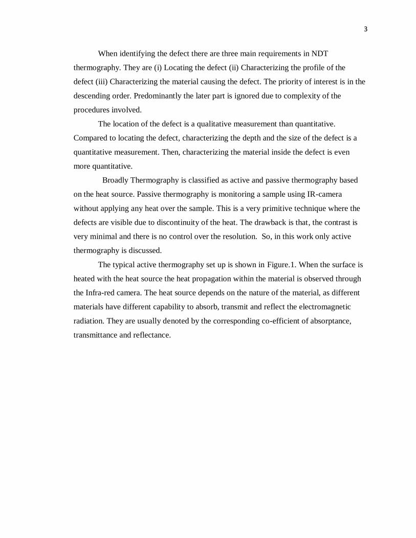
The typical active thermography set up is shown in Figure.1. When the surface is
heated with the heat source the heat propagation within the material is observed through
the Infra-red camera. The heat source depends on the nature of the material, as different
materials have different capability to absorb, transmit and reflect the electromagnetic
radiation. They are usually denoted by the corresponding co-efficient of absorptance,
transmittance and reflectance.

4
Figure.1.1 Typical Thermography set up of the sample and the IR camera
Active thermography can be broadly classified as (i) Pulse Thermography and (ii)
Lock-in Thermography. They are discussed below:
1.1.1. Pulsed Thermography. In Pulsed thermography [2, 3, 5, 15-17], the
sample to be inspected is heated on the surface by a heat source and is visualized by the
detector. Usually, the heat source is a flash lamp or Laser beam and the detector is an IR
Camera/detector.
Simple Pulse thermography set up is shown in the Figure.2.The source is a
halogen flash lamp which is switched ON and OFF for short period of time. The source
emits a short pulse of thermal energy Q over the surface.
Figure.1.2 Experimental Set-Up of the Pulse Thermography

5
The governing equation is given by Equation (2), assuming that the body is semi-
infinite where z the depth from the surface is Infinite. Effusivity of the body over the
time period t is defined by e .
( 0, )Q
T z te t
(2)
In the Figure.1.2, the surface temperature rise is plotted over time t at a specific
location. Each specific location yields a temperature time history. There is a difference
between the sample location without the defect and with defect. This is shown in
qualitative seen in the Figure.1.3. The thermograph will show uniform heat propagation
over the surface at T =0 when the sample doesn’t have a defect. The thermograph will
show the development of hot spot when there is a defect in the sample. This defect is in
fact creating a resistance to the thermal wave propagation and there is an accumulation of
thermal energy. This usually, is seen as a hot spot which is contrasting from the
background. The thermal contrast is given by the Equation (3) where 't is the time when
no defect is found. ( )dT t is the temperature at the defect at time t .
'
( ) ( ')dt
T T t T tt
(3)
6
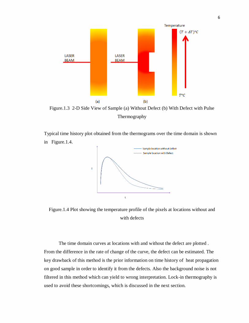
Figure.1.3 2-D Side View of Sample (a) Without Defect (b) With Defect with Pulse
Thermography
Typical time history plot obtained from the thermograms over the time domain is shown
in Figure.1.4.
Figure.1.4 Plot showing the temperature profile of the pixels at locations without and
with defects
The time domain curves at locations with and without the defect are plotted .
From the difference in the rate of change of the curve, the defect can be estimated. The
key drawback of this method is the prior information on time history of heat propagation
on good sample in order to identify it from the defects. Also the background noise is not
filtered in this method which can yield to wrong interpretation. Lock-in thermography is
used to avoid these shortcomings, which is discussed in the next section.

7
1.1.2 Lock-In Thermography. Lock-in thermography is yet another active
thermography which is widely used to identify the defects precisely in composites,
stainless steel, etc. [6, 18-22]. In this technique the source is a periodic heating element.
Usually, it is a Halogen lamp or a Laser depending on the sample under investigation and
the amount of heat required.
Figure.1.5 Conventional experimental set up of the Lock-in thermography
A simple Lock-in Thermography set up is shown in Figure.1.5. The periodic
heating of the surface is captured through the IR camera. The signal from the camera is
locked in to the frequency of the source. This enables to filter the noise and see the
periodic variation corresponding to the source frequency. From the signal, by performing
a Fast Fourier Transform the amplitude A and phase of the signal is identified and
mapped out for each pixel.
From the heat transfer perspective, the physics is explained briefly as below. The
fundamental math of the periodic heat source is given by the Equation (4), which is
introduced by Carslaw.H.S[23].The heat propagation is governed by the heat equation
shown in Equation (4). Heat equation explains the thermal diffusivity .On applying the
8
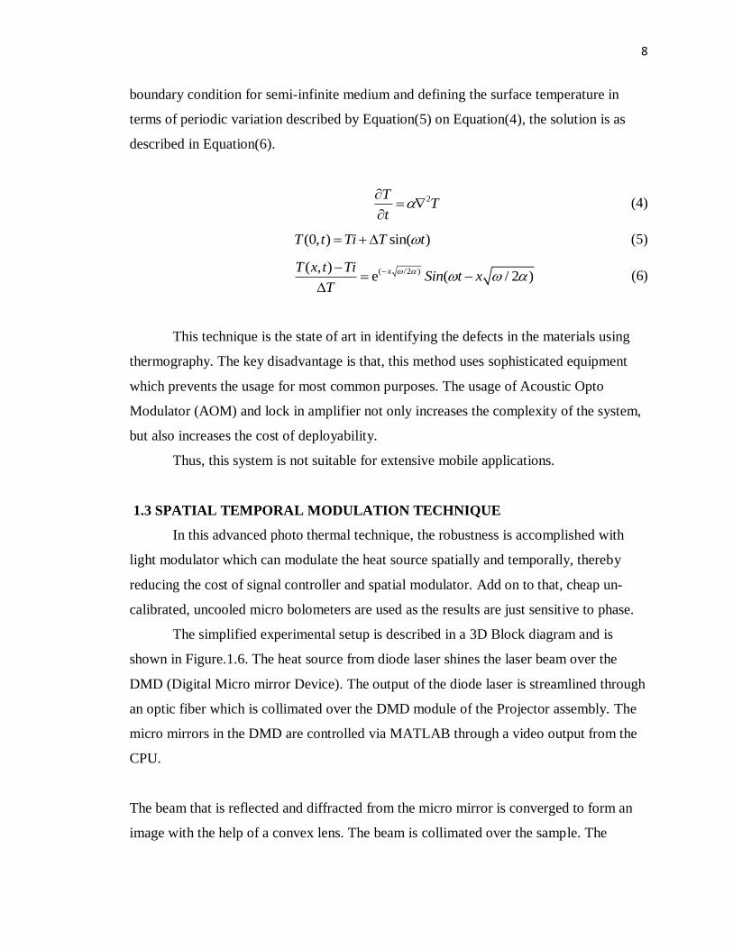
boundary condition for semi-infinite medium and defining the surface temperature in
terms of periodic variation described by Equation(5) on Equation(4), the solution is as
described in Equation(6).
2TT
t
(4)
(0, ) sin( )T t Ti T t (5)
( /2 )( , )e ( / 2 )
xT x t TiSin t x
T
(6)
This technique is the state of art in identifying the defects in the materials using
thermography. The key disadvantage is that, this method uses sophisticated equipment
which prevents the usage for most common purposes. The usage of Acoustic Opto
Modulator (AOM) and lock in amplifier not only increases the complexity of the system,
but also increases the cost of deployability.
Thus, this system is not suitable for extensive mobile applications.
1.3 SPATIAL TEMPORAL MODULATION TECHNIQUE
In this advanced photo thermal technique, the robustness is accomplished with
light modulator which can modulate the heat source spatially and temporally, thereby
reducing the cost of signal controller and spatial modulator. Add on to that, cheap un-
calibrated, uncooled micro bolometers are used as the results are just sensitive to phase.
The simplified experimental setup is described in a 3D Block diagram and is
shown in Figure.1.6. The heat source from diode laser shines the laser beam over the
DMD (Digital Micro mirror Device). The output of the diode laser is streamlined through
an optic fiber which is collimated over the DMD module of the Projector assembly. The
micro mirrors in the DMD are controlled via MATLAB through a video output from the
CPU.
The beam that is reflected and diffracted from the micro mirror is converged to form an
image with the help of a convex lens. The beam is collimated over the sample. The

9
sample is said to be semi-infinite when the thickness of the sample is more than 5 times
the thermal penetration depth. The thermal penetration depth or the thermal diffusion
length is the length of the sample till which the heat wave reaches for a particular lock-in
frequency. It is usually denoted by ‘z’. It is a function of Thermal diffusivity, α and Lock-
in frequency, f. It is given by Equation (7),
zf
(7)
The image acquired from the thermal camera is processed through MATLAB.
The Fast –Fourier transform is performed to attain amplitude and phase information at
the lock in frequency. The slope of the phase map for a given material gives a relation
between the thermal properties of the material. Thus, the material can be identified in a
remote fashion. The DMD helps in performing similar to localized photo thermal
radiometry technique. With this multiple capabilities mobile system identification is
possible.
Figure.1.6 3-D Block Diagram representing the simplified experimental
set-up

10
Figure.1.7 The laser beam raster and pulse over the surface as per the
desired frequency
Thus this technique brings the best of both the world of NDT-Thermography and Photo
thermal radiometry.
1.4 MOTIVATION
There is a need to develop a system which can identify the defects and
discontinuities which are fine cracks both qualitatively and quantitatively in a remote,
non-destructive fashion in diverse fields like Military, Aerospace Industry, and
Electronics Industry etc. The qualitative method is applied in robust testing of surface
defects. Also there is a need to perform system identification based on thermal properties
which is robust and compact. The combination of spatial and temporal modulation of
point and line heat source helps in identifying the cracks. When this modulation is
performed similar to photo thermal radiometry the thermal diffusivity can be estimated.
From the slope of the phase roll the thermal diffusivity could be approximated there by
predicting or distinguishing between conductive and nonconductive surfaces.
In this work, the cost is limited due to elimination of multiple laser sources and
complex instrumentation like Acoustic Opto Modulator (AOM) and Lock-in Amplifier.
And more novelty is added by the use of Digital Micro-mirror Device (DMD) for spatial
temporal modulation of multiple heat sources at different frequencies. The whole
instrument is made cheap and robust with the help of uncooled micro bolometer which
weighs less than 30g.
11
1.5 THESIS OVERVIEW
In this thesis, the experimental design and demonstration of cost effective
instrument to perform spatial temporal modulation for advance thermography apart from
conventional thermography is discussed. Under advance thermography, the capability of
the instrument to identify surface cracks and capability to spatially modulate multiple
heat sources are discussed. Apart from thermography, principles of radiometry are also
demonstrated for system identification. Under system identification, distinguishing the
materials based on the thermal diffusivity is demonstrated and discussed.
The thesis is sliced into five major segments, namely, the Introduction, DMD
device and its architecture theoretical background and Numerical analysis, Thermal
property estimation, results with discussion and finally the conclusion with future scope
of the work.
In the first chapter the conventional thermography and spatial temporal
modulation thermography is discussed describing the fundamentals and scope of each
technique. Then, The need for this work and how it could lead to commercially used is
explained. In the second chapter, the DMD device along with its architecture is described.
Then, in the third chapter, the numerical analysis of 2-D models is described along with
the governing equation for pulse, lock-in thermography, the boundary conditions and the
procedure in making a numerical analysis using ANSYS Workbench is described. The
numerical work helps in understanding the physics of the problem and possible solution.
In the fourth chapter, the principles of photo radiometry along with the theory and
application are discussed. In chapter five, the results of all the experiments and numerical
simulation are discussed. The demonstration of all the techniques discussed is
demonstrated. The final chapter discusses about the conclusion along with future work. It
describes about three possible directions in which this work can be extended.

12
2. DMD DEVICE-ITS ARCHITECTURE AND CAPABILITIES
In this chapter the development of a new type of thermo graphic experiment is
presented. The experimental setup is described in detail. This apparatus can be used for
the conventional thermography techniques at micro scale using laser as heat source, as
well as significantly demonstrating the feasibility to identify cracks and thermal property
distinction for system identification using spatial temporal modulation experiments.
2.1 DMD DEVICE
Digital Micro mirror Device (DMD) was developed by Texas Instruments in 1987
as a part of digital light processing device [24] .This patented technology used to
manipulate the light at finer scale to project with higher resolution. It is used almost in
85% of the digital cinema projection and used to manipulate the power sources for
additive manufacturing. A DMD chip consists of thousands of individually addressable
aluminum mirrors each of which can be steered. This is an example of a commercially
successful Micro-Electro-Mechanical System (MEMS). One such individual micro
mirror architecture is shown in Figure. 2.1. The aluminum mirror is mounted on using a
yoke present in the electric field. It is a comparable technology with Liquid Crystal
Display (LCD) to project light in TV, Projectors etc. Although both have their own range
of advantages, for this experiment DMD is considered suitable.
Figure.2.1 Micro mirror architecture present in DMD[24, 25]

13
The experiments in this thesis use a DLP 0.55 XGA chipset. This is a 0.55 in.
diagonal micro mirror array, with 10.8μm Micro mirror pitch [26] having 1024 x 768
pixels. Each mirror can deflect either -12 or +12°, with the -12°off the axis is considered
OFF and +12° off the axis is considered ON. The ON state projects the light at the
desired output location, whereas OFF state projects it on the heat sink to dissipate the
power. A compact cooling system with heat sink mounting along with radial fan is
present, as the maximum temperature it can withstand is between 80˚C to 90˚C. Since,
the mirrors are articulated under the electric field, they can be modulated as high as 80
kHz digitally. The mirror which is capable of flipping to ON and OFF states at such
frequencies can produce 1024 shades of grey. This different shades of grey is
synchronized with the color wheel to produce the appropriate color of the input image.
But, as for this experiment is concerned, the color wheel is redundant and is isolated from
the circuit. This range enables the experimenter to manipulate the laser beam either to
direct it towards the sample or towards a sink. When a single micro mirror is modulated
at a specific frequency, the laser beam is modulated at the same frequency of the mirror.
When the consecutive mirrors are manipulated in a series, the laser beam is rastered over
the surface. This enables to perform spatial thermo reflectance. Both spatial and temporal
modulation is possible when the mirrors are manipulated simultaneously at specific
frequencies.
The CMOS Substrate receives the signal and manipulates the movement of micro
mirror. The projected light is collimated back to the sample surface using conventional
optics. The negative of the image is focused to the sink to absorb the remaining radiation.
The temperature variation due to periodic heat source is observed through uncooled
micro bolometer thermal camera. The data is recorded and processed in the computer
through MATLAB. Figure 2.2 illustrates the dimension of the Micro mirror Array
through SEM image taken at 500X.

14
Figure.2.2 SEM image of the Micro mirror Array[27]
2.2 EXPERIMENTAL SET UP.
The simplified experimental setup is shown in Figure.2.3 and is described in a 3D
Block diagram in Figure. 2.4. The heat source utilized in this experiment is a Coherent
DUO-FAP Diode Laser of 800 nm and 532nm wavelength with maximum power of 30W
each. Only one of the two outputs is used for this experiment. The diode output is
transmitted through a fiber optic cable which is collimated over the DMD module of the
Projector assembly. The DMD assembly is extracted from DELL 1409X Projector for
convenience. One of the lighter objectives of the experiment is to make the system robust
and cheap. In order to accomplish it, a hack was made in an old unused projector which
had burnt out lamp. The micro mirrors in the DMD are controlled via MATLAB through
a video output from the CPU. MATLAB code is used to generate videos of geometries
varying periodically at specific frequencies and is given at Appendix. These videos are
played in CPU and are passed on to DMD via VGA 15-pin connector cable. Figure.2.3
shows the Experimental set-up inside the shielded enclosure. The detailed block diagram
is illustrated in Figure. 2.4.

15
Figure.2.3 Experimental set up inside the shielded enclosure
Figure.2.4 Experimental setup where laser is collimated over the DMD array
2.3 CAPABILITIES OF THE DEVICE:
The device is capable of performing (i) Pulse, (ii) Lockin, thermography (iii)
spatial and temporal modulated thermography

16
2.3.1 Pulse Thermography. Pulse thermography as discussed earlier is a short
emission of laser radiation or heat flux on the sample. The short pulse is absorbed by the
surface, locally heating the first few micrometers. The thermal energy diffuses through
the sample via conduction and the surface begins to cool. In regions where the
conductivity is substantially different than the host media (e.g. an abscess, crack, or
buried metal trace) the conduction away from the surface is disrupted, which affects the
surface temperature. Deviations in the surface temperature can be observed with a
thermal camera and used to identify and locate defects in the sample. Usually in
conventional pulse thermography, the whole sample is pulsed with the flash lamp heat
source [2, 5, 21]. The flash lamps provide huge radiative heat flux and are cheaper
compared to laser source. In this work, the laser is used as it is a coherent, continuous
wave heat source which is directional with minimum loss. It is highly desired for the
spatial temporal modulation of the heat source, where precise control of heat flux is
necessary. Since, the location, shape and size of the defect are generally not known a
priority, it often takes multiple experiments to identify and qualitatively characterize a
defect [28].
With the help of DMD device, simultaneous pulsing can be done and also pulsing
of different flux density is possible by varying the area of the laser beam being projected.
It is illustrated in the Figure.2.5. The diameter of the pulse can be precisely controlled by
the DMD with the help of image generated by MATLAB.

17
Figure.2.5 Sample is pulsed at different diameter by the DMD Device
2.3.2 Lock-in Thermography. Lock-in thermography as mentioned earlier is
gives more quantification of the defect compared to the pulse thermography. But, the
conventional setup[19, 22] is expensive utilizing high end signal processing tools. The
signal processing is indeed necessary to increase the noise filtering capabilities, but with
the help of fast Fourier transform the image is processed in simple fashion at the lock in
frequency. In conventional setup in order to identify and characterize several lock in
frequencies need to be done sequentially and is a time consuming process[28]. Using the
DMD device, the pattern projected can be controlled based on the need and can perform
simultaneous lock in thermography which are discrete in spatial domain.
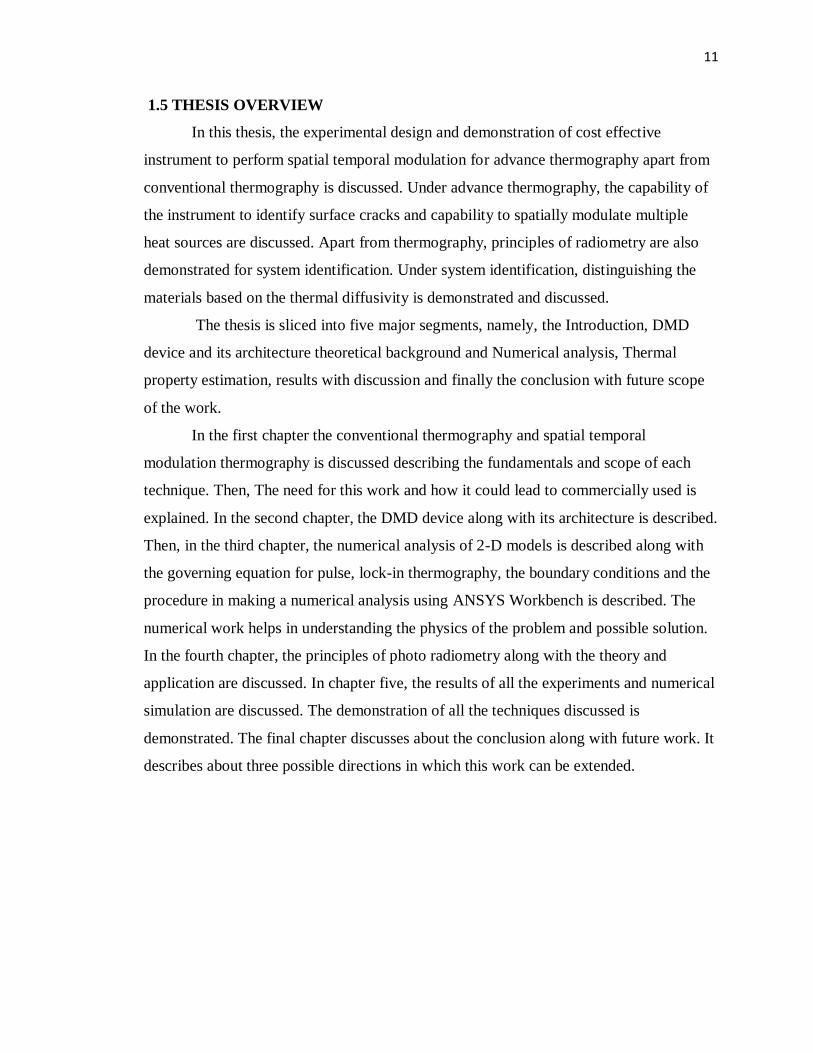
Figure.2.6 illustrates the use of the device to simultaneously lock in at multiple
frequencies as well as the possibility to lock-in with different profile. This is highly
useful in identifying cracks and performing localized lock in thermography in structures
like Wind Turbines or Aerospace structures where the whole sample cannot be
illuminated by the flash lamp for lock in thermography. Even when illuminated, it will be
insensitive to finer cracks. The pattern projected can be optimized for identifying the
defects in quicker fashion. It is a control and optimization problem by itself and is beyond
the scope of this work.
18
When lock in at different frequency is done, there is possibility of pulse
compression where the phase match of the neighboring heat wave occurs and forms a
pulse[29].
Figure.2.6 Sample is pulsed at different frequency and profile by DMD Device
2.3.3 Spatial and Temporal Modulation Thermography. Scanning the laser
beam is highly useful technique to identify the cracks or defects in XY plane. As the laser
beam is probed over the surface, the discontinuity acts as a non-conducting medium
preventing the heat transfer along XY plane. This creates a heat spot and can be highly
useful for quick evaluation of the defect. This defect is difficult to evaluate using
conventional pulse or lock-in thermography. Comparing the conventional pulse, lock in
thermography techniques this requires a different set up and is usually done with the help
of laser beam[30].
The DMD device developed in this work is robust to perform the scanning laser
beam technique to identify the defects in the cross plane as shown in Figure.2.7. The
moving laser beam is manipulated by the movie created using MATLAB. The location,
the rate of scanning and the diameter of the profile is controlled precisely by MATLAB.

19
Instead of just one spatially modulated beam, the beam can be temporally
modulated to be immune from the DC noise affecting the signal. The spatially and
temporally modulated beam has higher sensitivity to crack which is not detected under
conventional flash or lock-in thermography[31]. For a larger area, multiple point or line
heat source can be modulated spatially and temporally to identify the crack. The signal
from the whole surface is locked in at all the corresponding lock-in frequency.
Figure.2.7 Sample is probed by scanning laser beam by DMD Device
Figure.2.8 Temporal Modulation by DMD Device by different frequencies
20
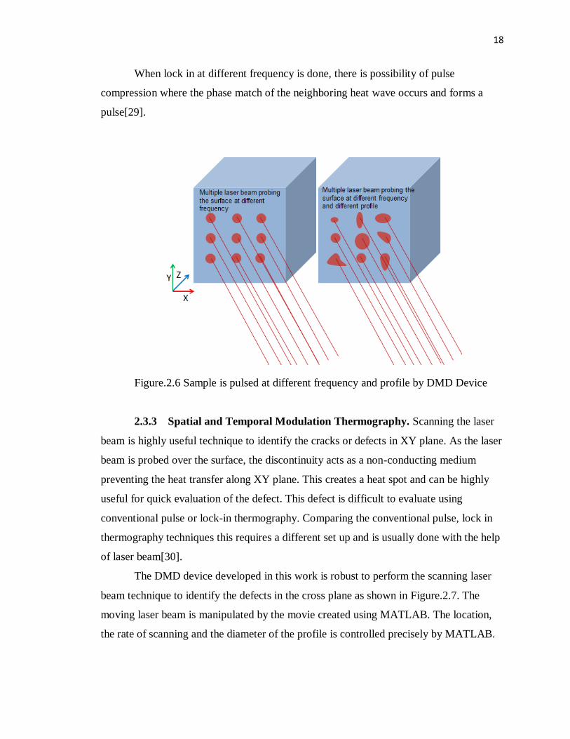
2.4 LINEAR CO-ORDINATE TRANSFORMATION
The co-ordinate linear transformation is a mathematical tool to map the desired
set from one plane to the other[32]. In this experiment, the camera which is parallel to the
plane of the sample would observe a skewed image from the DMD projector. For the ease
of analysis, a proper geometry would be helpful. In order to facilitate it, the linear
transformation is used to find the skewed image which can project a proper geometry on
the plane of the sample. It is shown in Figure.2.9 and the general equation of the
transformation is shown in Eq.8. In this equation, transformation T maps the geometry
from (u,v) plane to (x,y) plane.
(u, v) = x (u,v),y (u, v)T (8)
Figure.2.9 Linear Co-ordinate transformation mapping from the computer to the
sample
The following is a detailed mathematical description of the process. In this
experiment, there are two planes under discussion. One is the plane in the computer
graphics which controls the DMD, the other is the projected image plane. For ease, the
earlier one is called control plane and the other one is called projected plane. The co-
ordinate points of the rectangle in control plane are namely ( 1x , 1y ),( 2x , 2y ),( 3x , 3y ) and (

21
4x , 4y ) as shown in Figure.2.10. Similarly, the points in the projected plane are called ( 1i
, 1j ),( 2i , 2j ),( 3i , 3j ) and ( 4i , 4j ).
Figure.2.10. Mapping of co-ordinates between different planes
The simple transform equation for first point would be:
1 1
1 1
x ia b
c d y j
(9)
Similarly, there are three more set of linear equations.
2 2
2 2
x ia b
c d y j
(10)
3 3
3 3
x ia b
c d y j
(11)
4 4
4 4
x ia b
c d y j
(12)
Solving any of these four simultaneous equations the constants a, b, c, d can be
found.

22
The co-ordinates of the desired geometry which needs to be projected in the
projected plane are already known as it is the desired parameter. In this case, let those co-
ordinates be ( '
1i , '
1j ),( '
2i , '
2j ),( '
3i , '
3j ) and ( '
4i , '
4j ) respectively. Using the transformation
constants a, b, c, d and the new desired control points ( '
1x , '
1y ) can be found. It is shown
in Eq. (13). Likewise the other new co-ordinates can be found
.
1' '
1 1
' '
1 1
x i a b
c dy j
(13)
23
3. NUMERICAL ANALYSIS
In this chapter, the details of the numerical model are explained. Transient
thermal problems are always complex and unpredictable. This complexity is one of the
key obstacles in understanding the heat transfer propagation in the material which
evolves in space and time. As direct analytical models are even more complex to capture
all the dynamics and boundary conditions, numerical models are preferred to be used.
Numerical model helps to understand the physics behind the experiment and enables to
foresee the results. It also enables us to perform parametric and optimization studies
beforehand.
In order to perform, numerical analysis Finite Element Method (FEM) is used.
FEM is one of the most popular numerical techniques to perform transient heat transfer
simulations. It has the versatility to handle material non linearity and nonlinear boundary
conditions. ANSYS Workbench is used for this project as it is one of the well-established
FEM solver used to perform multi-physics simulations.
The experiment verifies the numerical model and the explanation for any offset
behaviors are explained.
3.1 GOVERNING EQUATION
The experiment involves all the three forms of heat transfer like Conduction,
Convection and Radiation. Radiation is considered negligible or has been accommodated
in the model if found to have reasonable contribution. The model generated is a 2-D
approximation numerical model where Z<<(X, Y). So the conduction along XY plane is
high compared to YZ plane.
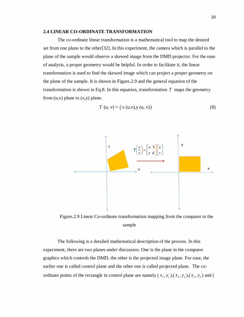
Equation (3) is the heat conduction diffusion equation derived from Fourier law of
heat conduction where the heat diffusion along x, y, z is represented. For pulse
thermography, Equation (14) & (15) are applied to the elements where the heat pulse is
applied. For the elements where no heat is applied Equation(16) is applied.
2TT
t
(4)

24
Where x y z
When [0, ]pulsetime time
4 4
0 ( ) ( )conv amb amb
T T Tk q h T T T T
x y z
(14)
When [ , ]pulse endtime time time
4 4( ) ( )conv amb amb
T T Tk h T T T T
x y z
(15)
The elements where heat is not applied, [0, ]endtime time
4 4( ) ( )conv amb amb
T T Tk h T T T T
x y z
(16)
For lock-in thermography, the input heat q0 in Equation (14) is modified to periodic
function as shown in Equation (17), where Q is the peak power during the period. The
element where the heat is applied is similar to pulse thermography.
(1 cos( )2
Qq t (17)
The temperature distribution for periodic heat source is already discussed with the help of
Equation (5) and (6) under lock-in thermography section.
(0, ) sin( )T t Ti T t (5)
( /2 )( , )e ( / 2 )
xT x t TiSin t x
T
(6)
/ ( * )pk C , and 2

25
3.2 BOUNDARY CONDITION
The model has three types of boundary conditions: Firstly, Heat flux with
convection and radiation, Secondly, Convection with constant temperature Thirdly,
Convection with radiation. The heat flux with convection is applied on the top surface
where the laser beam is projected. From experiment, the Heat flux is measured to be
within the range of 500 to 1000W/m2. Convection boundary condition is implied on all
the 18 faces of the sample which includes the surface area covered by the defects.
Convection co-efficient of 10 W/m2.˚C is applied along these faces subjected to standard
atmospheric temperature and pressure. Second type of boundary condition is applied on
the base of the model, to simulate real time conditions. All other sides have third type of
boundary condition. Radiation is applied if the sample under investigation has high
emissivity. The samples are either black in color or are subjected to a black coat to
maximize the absorptivity. This is would just influence the amplitude of the signal and is
insensitive to phase.
3.3 FINITE ELEMENT MODELING
3.3.1. Geometric Modeling. In order to simulate the physics, 2D approximation
of the sample is created to reduce computational time and for straight forward description
of the results. Geometric modeling is performed using the Design Modeler in the ANSYS
Workbench 14. The dimension of the sample is shown in Figure.3.1. The design has been
parametrized for future optimization. The named selection has been created to apply load
and boundary condition as shown in Figure.3.2.
Figure.3.1 Dimension of the sample as made in Design Modeler of Ansys
Workbench 14.
3.8 mm
20 mm
3.5 mm 2mm

26
Named Selection- To define the segment where laser beam can be applied
Edge Refinement in the Area of Interest
Figure.3.2 Named Selection in the geometric modeling to specify Thermal load
3.3.2. Meshing. The next immediate process in the finite element modeling
procedure is to define the mesh volumes. So the geometry is sub divided into smaller
finite volumes. Tetrahedron mesh is applied to the body and finer refinement is applied in
the places of defects where changes in temperature are of primary interest. The mesh with
edge refinement is shown in Figure.3.3 and the setting is shown in Figure.3.4.
Figure.3.3 Tetrahedron Mesh with fine refinement on the area of interest
27
Figure.3.4. Mesh Setting
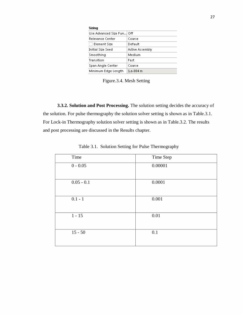
3.3.2. Solution and Post Processing. The solution setting decides the accuracy of
the solution. For pulse thermography the solution solver setting is shown as in Table.3.1.
For Lock-in Thermography solution solver setting is shown as in Table.3.2. The results
and post processing are discussed in the Results chapter.
Table 3.1. Solution Setting for Pulse Thermography
Time Time Step
0 - 0.05
0.00001
0.05 - 0.1
0.0001
0.1 - 1 0.001
1 - 15
0.01
15 - 50 0.1

28
Table 3.2. Solution Setting for Lock-in Thermography
Time Time Step
0-15 .01

29
4. RESULTS
This chapter is split up into two sections. First section discusses the numerical
results which describes the existence of the problem and predicts the solution to the
problem statement. The later discusses about the experimental results. The experimental
results consist of conventional pulse, lock in thermography, material property estimation
for system identification, crack detection using spatial temporal modulation and
application of simultaneous spatial temporal modulation.
4.1 NUMERICAL RESULTS
In this section, 2-D approximated Numerical models have been simulated and the
results are discussed. The numerical simulation of conventional pulse thermography,
lock-in thermography and spatial temporal modulation for crack identification are
discussed. The simulation helps in understanding the physics of the problem and possible
solution. The material property used in this model is FR-4.The thermal property used for
the numerical simulation is shown in Table.4.1.
Table.4.1 Properties of FR-4 used in the simulation
Thermal Property Value, units
Thermal Conductivity in W/m.K 0.294
Density in kg/m3 1900
Specific heat capacity, kJ/kg.K 1150
30
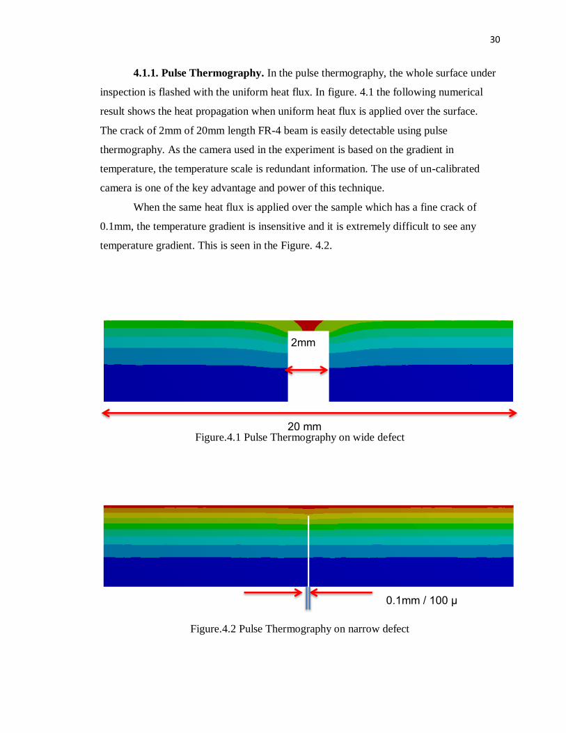
4.1.1. Pulse Thermography. In the pulse thermography, the whole surface under
inspection is flashed with the uniform heat flux. In figure. 4.1 the following numerical
result shows the heat propagation when uniform heat flux is applied over the surface.
The crack of 2mm of 20mm length FR-4 beam is easily detectable using pulse
thermography. As the camera used in the experiment is based on the gradient in
temperature, the temperature scale is redundant information. The use of un-calibrated
camera is one of the key advantage and power of this technique.
When the same heat flux is applied over the sample which has a fine crack of
0.1mm, the temperature gradient is insensitive and it is extremely difficult to see any
temperature gradient. This is seen in the Figure. 4.2.
Figure.4.1 Pulse Thermography on wide defect
Figure.4.2 Pulse Thermography on narrow defect
20 mm
2mm
0.1mm / 100 μ
31
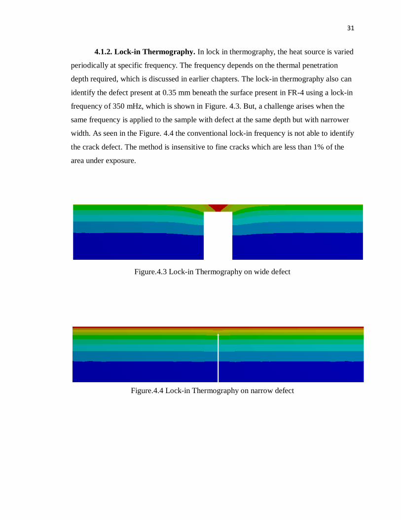
4.1.2. Lock-in Thermography. In lock in thermography, the heat source is varied
periodically at specific frequency. The frequency depends on the thermal penetration
depth required, which is discussed in earlier chapters. The lock-in thermography also can
identify the defect present at 0.35 mm beneath the surface present in FR-4 using a lock-in
frequency of 350 mHz, which is shown in Figure. 4.3. But, a challenge arises when the
same frequency is applied to the sample with defect at the same depth but with narrower
width. As seen in the Figure. 4.4 the conventional lock-in frequency is not able to identify
the crack defect. The method is insensitive to fine cracks which are less than 1% of the
area under exposure.
Figure.4.3 Lock-in Thermography on wide defect
Figure.4.4 Lock-in Thermography on narrow defect
32
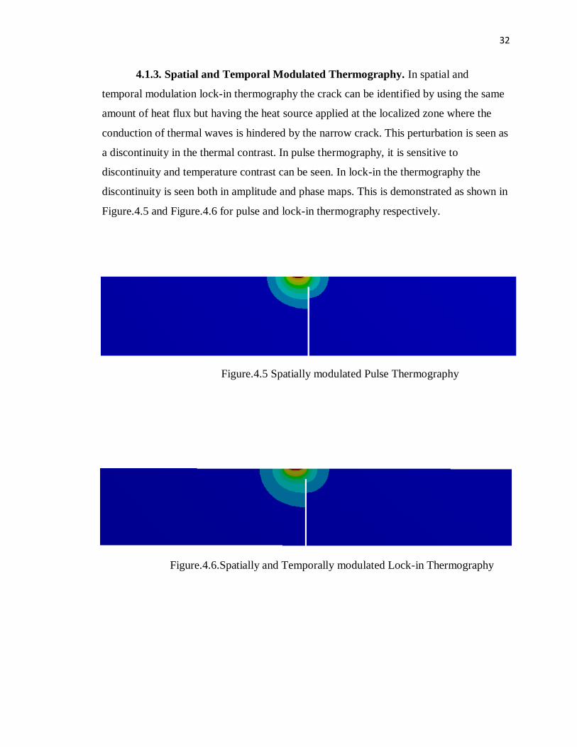
4.1.3. Spatial and Temporal Modulated Thermography. In spatial and
temporal modulation lock-in thermography the crack can be identified by using the same
amount of heat flux but having the heat source applied at the localized zone where the
conduction of thermal waves is hindered by the narrow crack. This perturbation is seen as
a discontinuity in the thermal contrast. In pulse thermography, it is sensitive to
discontinuity and temperature contrast can be seen. In lock-in the thermography the
discontinuity is seen both in amplitude and phase maps. This is demonstrated as shown in
Figure.4.5 and Figure.4.6 for pulse and lock-in thermography respectively.
Figure.4.5 Spatially modulated Pulse Thermography
Figure.4.6.Spatially and Temporally modulated Lock-in Thermography
33
4.2 EXPERIMENTAL RESULTS
Experiments have been performed demonstrating conventional pulse
thermography, lock-in thermography, crack-detection and finally the capability to
perform multiple spatial and temporal thermography.
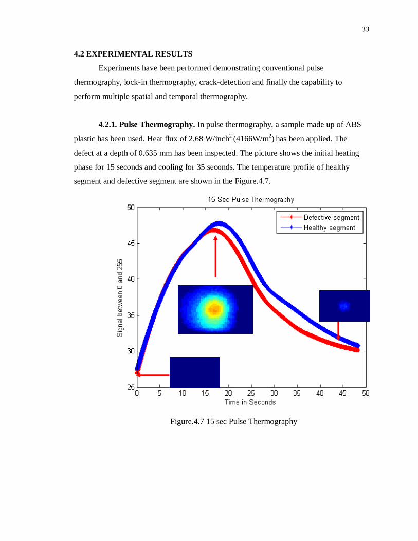
4.2.1. Pulse Thermography. In pulse thermography, a sample made up of ABS
plastic has been used. Heat flux of 2.68 W/inch2 (4166W/m
2)
has been applied. The
defect at a depth of 0.635 mm has been inspected. The picture shows the initial heating
phase for 15 seconds and cooling for 35 seconds. The temperature profile of healthy
segment and defective segment are shown in the Figure.4.7.
Figure.4.7 15 sec Pulse Thermography

34
-- Location 1 -- Location 2
-- Location3
4.2.2. Lock-in Thermography. In lock-in thermography the defect of 2.54mm
diameter at a depth of 0.635mm is used to demonstrate the lock-in thermography
capability. Although a uniform heat flux is applied, the heat conduction is hindered in the
defective area and gets accumulated resulting in temperature rise. This is reflected in the
amplitude and phase map. After performing FFT of the signal, the amplitude and phase
map at 97.5 mHz is illustrated as shown in Figure.4.8. The temperature variation at the
location 1,2 and 3 is shown in the Figure.4.8. The decrease in amplitude and marginal
shift in phase can be seen in Figure4.9 due to the presence of defect. The FFT of the
thermal wave is plotted on the right in Figure.4.9.
Fig Amplitude and Phase image of Lock in Thermography
4.1.1 Spatial and Temporal Modulated Lock-in for Crack Identification:
Figure.4.8 Amplitude and Phase image of the defective ABS sample
Figure.4.9 FFT plot and the location of defects as shown in Figure.4.8
1 2 3
35
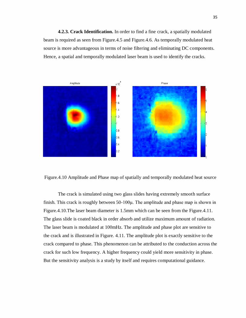
4.2.3. Crack Identification. In order to find a fine crack, a spatially modulated
beam is required as seen from Figure.4.5 and Figure.4.6. As temporally modulated heat
source is more advantageous in terms of noise filtering and eliminating DC components.
Hence, a spatial and temporally modulated laser beam is used to identify the cracks.
Figure.4.10 Amplitude and Phase map of spatially and temporally modulated heat source
The crack is simulated using two glass slides having extremely smooth surface
finish. This crack is roughly between 50-100μ. The amplitude and phase map is shown in
Figure.4.10.The laser beam diameter is 1.5mm which can be seen from the Figure.4.11.
The glass slide is coated black in order absorb and utilize maximum amount of radiation.
The laser beam is modulated at 100mHz. The amplitude and phase plot are sensitive to
the crack and is illustrated in Figure. 4.11. The amplitude plot is exactly sensitive to the
crack compared to phase. This phenomenon can be attributed to the conduction across the
crack for such low frequency. A higher frequency could yield more sensitivity in phase.
But the sensitivity analysis is a study by itself and requires computational guidance.

36
Width of the crack
Figure.4.11 Amplitude and Phase segment transverse to the crack
4.2.4. Multiple Spatial and Temporal Modulations. As discussed in the
previous section, the identification of crack requires a localized spatial temporal
modulation. This is a cumbersome process to follow when the area under scanning is of
higher order in magnitude compared to the crack. Unfortunately, the reality is that the
cracks are always going to be finer and be several orders lower from the actual dimension
of the sample. In order to perform the search for cracks multiple spatial temporal
modulation is required. This is enabled with the help of DMD and is demonstrated by
having two line heat sources being periodic and spatially apart from each other. One line
of 1Hz and other with 2Hz is pulsing periodically on the cu-cladding of FR-4 surface.
The raw and the processed image on color scale are illustrated in Figure.4.12.

37
Figure.4.12 Segment of Raw signal from the DRS camera and the corresponding color
image
Figure.4.13.FFT plot of each line
Figure.4.14.Amplitude and Phase plot corresponding to 1Hz and 2Hz
38
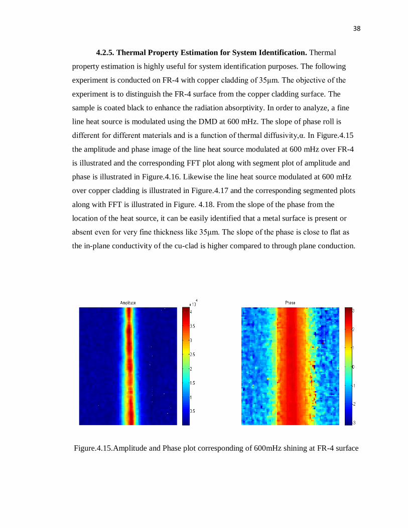
4.2.5. Thermal Property Estimation for System Identification. Thermal
property estimation is highly useful for system identification purposes. The following
experiment is conducted on FR-4 with copper cladding of 35μm. The objective of the
experiment is to distinguish the FR-4 surface from the copper cladding surface. The
sample is coated black to enhance the radiation absorptivity. In order to analyze, a fine
line heat source is modulated using the DMD at 600 mHz. The slope of phase roll is
different for different materials and is a function of thermal diffusivity,α. In Figure.4.15
the amplitude and phase image of the line heat source modulated at 600 mHz over FR-4
is illustrated and the corresponding FFT plot along with segment plot of amplitude and
phase is illustrated in Figure.4.16. Likewise the line heat source modulated at 600 mHz
over copper cladding is illustrated in Figure.4.17 and the corresponding segmented plots
along with FFT is illustrated in Figure. 4.18. From the slope of the phase from the
location of the heat source, it can be easily identified that a metal surface is present or
absent even for very fine thickness like 35μm. The slope of the phase is close to flat as
the in-plane conductivity of the cu-clad is higher compared to through plane conduction.
Figure.4.15.Amplitude and Phase plot corresponding of 600mHz shining at FR-4 surface
39
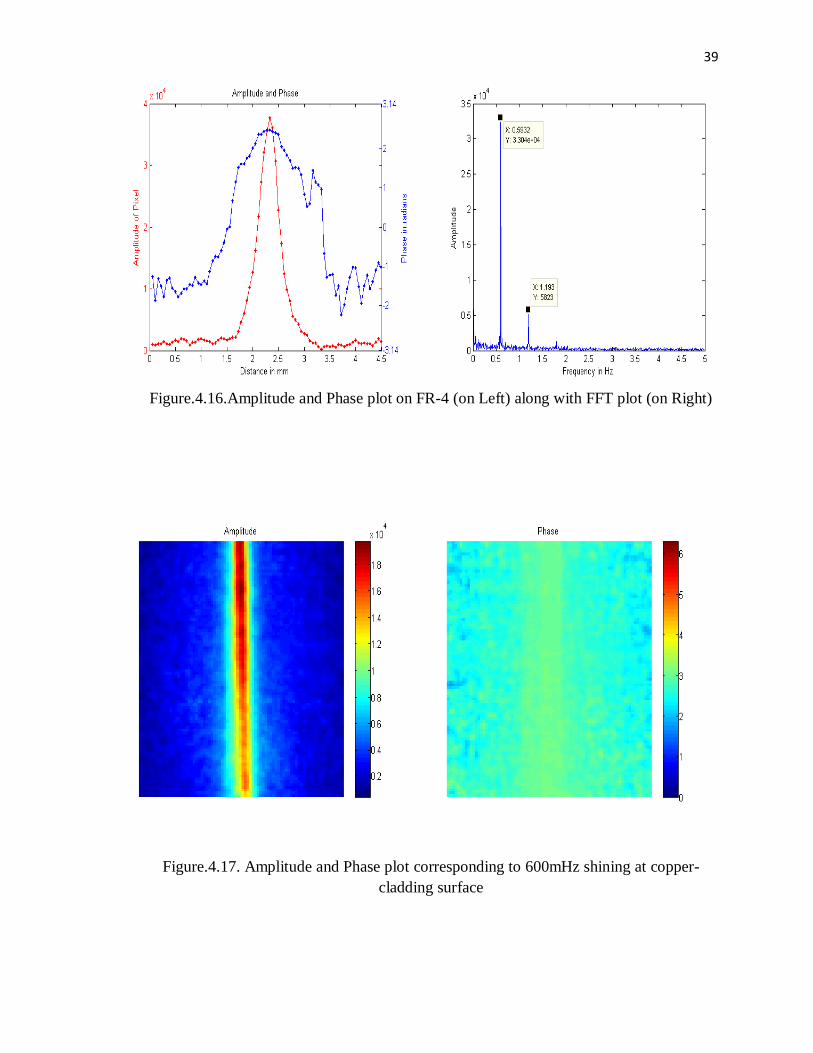
Figure.4.16.Amplitude and Phase plot on FR-4 (on Left) along with FFT plot (on Right)
Figure.4.17. Amplitude and Phase plot corresponding to 600mHz shining at copper-
cladding surface

40
Figure.4.18.Amplitude and Phase plot on Copper cladding (on Left) along with FFT plot
(on Right)
41
5. CONCLUSION AND FUTURE WORK
5.1 CONCLUSION
Non-Destructive Testing (NDT) is highly essential in improving the confidence in
quality of the products. With humongous product lines in today’s industry there is a need
to perform simultaneous NDT techniques. The device built in this work enables to work
towards that goal. The instrument’s capability to perform (i) Pulse thermography, (ii)
Lock-in thermography (iii) spatially and temporally modulated thermography were
demonstrated. The need to quantify the defect using advancement in thermography was
realized and a device was fabricated in that direction. The capability of the device was
established. The application of these principles to future work is discussed as under.
5.2. FUTURE WORK
The future work is really interesting as plenty of opportunities are ahead. The
future work is broadly classified under three directions. Firstly, based on the
thermography technique for crack detection, Secondly, based on system identification
using the thermal property distinction, Thirdly, based on the application of the system to
diverse areas in order to solve commercial challenges.
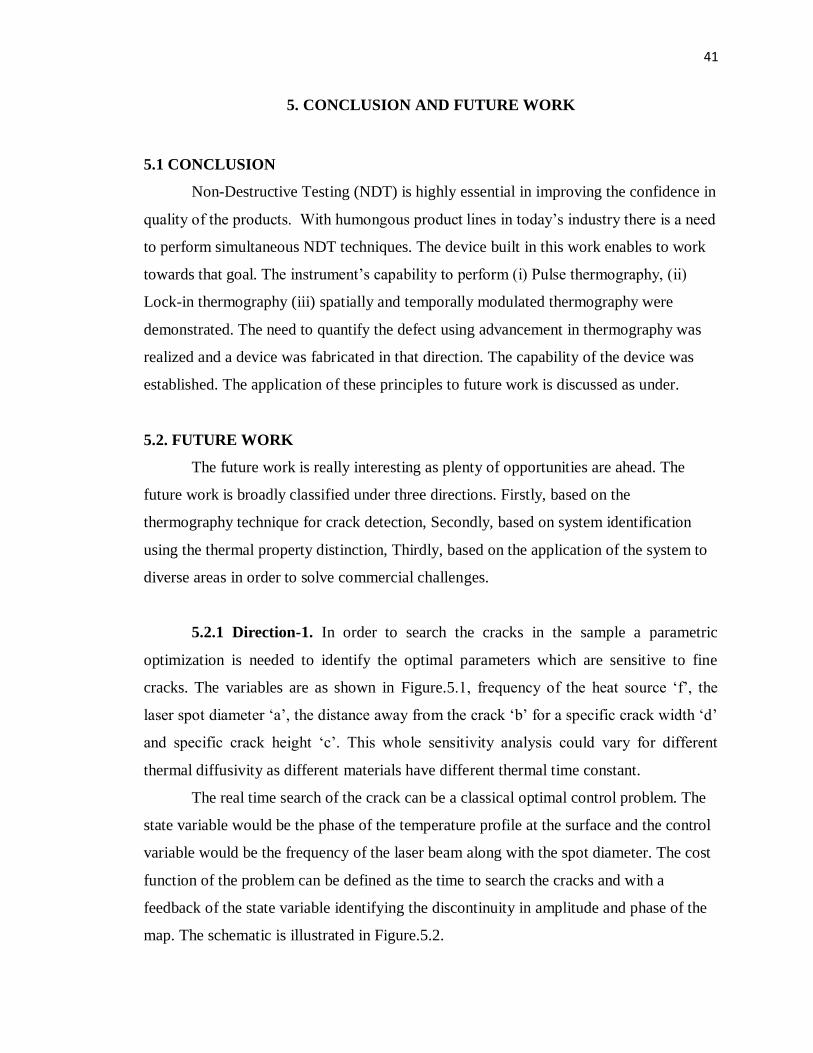
5.2.1 Direction-1. In order to search the cracks in the sample a parametric
optimization is needed to identify the optimal parameters which are sensitive to fine
cracks. The variables are as shown in Figure.5.1, frequency of the heat source ‘f’, the
laser spot diameter ‘a’, the distance away from the crack ‘b’ for a specific crack width ‘d’
and specific crack height ‘c’. This whole sensitivity analysis could vary for different
thermal diffusivity as different materials have different thermal time constant.
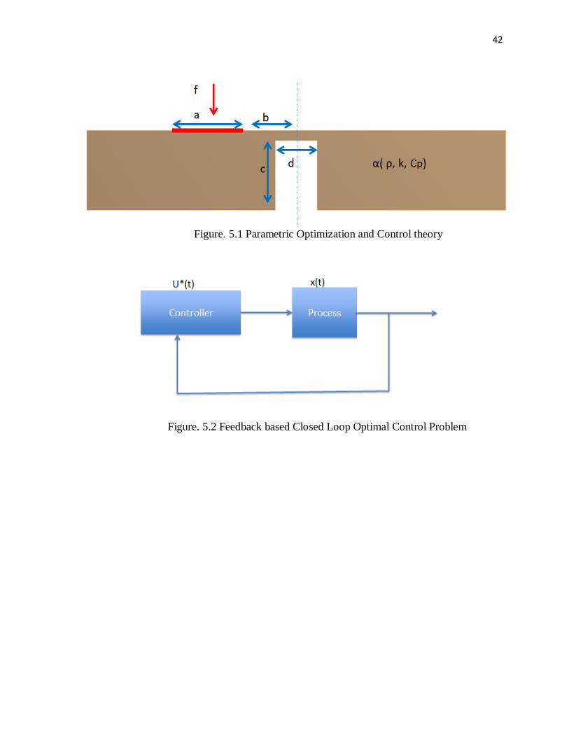
The real time search of the crack can be a classical optimal control problem. The
state variable would be the phase of the temperature profile at the surface and the control
variable would be the frequency of the laser beam along with the spot diameter. The cost
function of the problem can be defined as the time to search the cracks and with a
feedback of the state variable identifying the discontinuity in amplitude and phase of the
map. The schematic is illustrated in Figure.5.2.
42
Figure. 5.1 Parametric Optimization and Control theory
Figure. 5.2 Feedback based Closed Loop Optimal Control Problem

43
5.2.2 Direction-2. The current technique is useful in identifying and
distinguishing materials based on the thermal properties. The value addition to the
technique would be generating 3-D profile of the geometry along with the thermal data
imbibed in them for better understanding of the sample. The sample can be scanned by
projecting optical fringes using similar DMD light modulator and the scattered distorted
light can be captured using two simultaneous CCD cameras placed at known perspective
from the sample. Thus, the captured light could be reconstructed to form 3D image as
shown in Fig.5.3. As the lockin technique is insensitive to orientation and illumination,
the thermal property information along the surface could be imbibed to the 3D model.
Figure.5.3 Structured light 3D scanner scanning a car seat to generate 3-D profile
[33]
5.2.3 Direction-3. The third direction would be to apply the technique in solving
challenges of commercial interests. One great application for different commercial
problems:
Deploying in autonomous mobile systems to identify obstacles while performing
rescue operations. Deploying in system with a conveyor system to identify cracks and
defects demonstrating for industries like electronics industry(Find cracks in circuits,
defects in soldering or printing of circuits), fuel cell industry (To detect cracks in graphite
plates which are expensive during pre and post manufacturing conditions).

44
Currently, the DMD used in the experiment can handle only a maximum of 50W.
It can be enhanced by arranging multiple DMDs to cover a larger area and the search for
cracks in large samples would be feasible. Also fine resolution of DMD can provide
higher resolution of thermal projections which can improve the sensitivity.

45
APPENDIX
To control the experiment, multiple MATLAB codes were written. These codes perform
the following tasks:
A. To control the laser
B. To generate videos of specific frequency or pattern to manipulate the DMD
C. To post process Lock-in Thermography video
D. To post process Pulse Thermography video
E. To post process the amplitude and phase result to create GIF movie
MATLAB CODES TO CONTROL LASER
In order to communicate with the laser an ‘object’ has to be created and string values
needs to be passed on to them.
The following code creates an object called ‘laser’ to which string values can be passed
on. The user can change the port to COM1 or COM2 depending on the availability. The
string ‘01o1’ controls laser 1 and string ‘02o1’ controls laser 2. This is applicable for all
similar commands where the appropriate laser needs to be addressed.
%%%START%%%
laser = instrfind('Type', 'serial', 'Port', 'COM3', 'Tag', '');
if isempty(laser)
laser = serial('COM3');
else
fclose(laser);
laser = laser(1);
end
set(laser, 'Terminator', [1]);
set(laser, 'Timeout', 5.0);
fopen(laser);
%%%
Laser Status Control
%%%START%%%
fprintf(laser,'01o0'); % Switch OFF
fprintf(laser,'01o1'); % Switch ON and Get Ready
fprintf(laser,'01o2'); % Active and Fire

46
%%%END%%%
The following is the code to control the laser to vary the power periodically for specific
frequency.
The first part of the code creates the sine wave form and the second part uses the data to
manipulate the power according to the data. The waveform generated is passed on to the
laser as string. A minute pause is created for the hardware to respond. This will have
negligible effect, as the maximum frequency in this experiment is 15Hz due to nyquist
limitation.
% First Part%
%%%START%%%
Fs=30;% Sampling rate (Lower sampling rate for lower frequency and higher sampling
rate for higher frequency)
fz=0.5;% Frequency of the signal
dt=1/Fs;
TotalTime=10;
t=(0:dt:TotalTime-dt);
x=2500+1500*sin(2*pi*fz*t); % Defining the range of power
y=int32(x); % Converting to Integer
figure
plot(t,x,'-*')
xlabel('Time in Seconds');
title('Wave');
[~,n]=size(y);
% Second part
fprintf(laser, '01o0');
fprintf(laser, '01o1');
pause(2)
fprintf(laser,'01o2');
for i=1:n
k=num2str(y(1,i));
fprintf(laser,'01p0[;%s]\r',k);
pause(.00005)
end
fprintf(laser, '01o1');
%%%END%%%

47
MATLAB CODE TO GENERATE VIDEOS TO MANIPULATE DMD
Create a line scan video for scanning laser beam thermography
The following code enables to create a vertical line and move it. This video is generated
to scan the surface with the laser beam. The user has control of the rate at which the line
can move, the length of the line and the overall size of the plot area, the thickness of the
line. The sampling rate helps in controlling the rate at which the line can move, the
‘LineWidth’ helps in controlling the thickness of the line.
%%%START%%%
writerObj = VideoWriter('output.avi');
open(writerObj);
x1=(1:.25:50);
x2=(1:.25:50);
y1=1;
y2=100;
[~,no]=size(x1);
for i=1:no
drawnow
plot([x1(i),x2(i)],[y1,y2],'Color','black','LineWidth',6)
set(gca,'XLim',[0 50], 'YLim',[0 100]);
set(gca, 'xtick', [], 'ytick', []) ;
set(gcf,'color','w');
set(gca, 'xcolor', 'w', 'ycolor', 'w');
drawnow
frame = getframe(1);
writeVideo(writerObj,frame);
end
close(writerObj);
%%%
The following code enables to create a horizontal line and move it. This video is
generated to scan the surface with the laser beam. It is similar to the code above.
%%%START%%%
clear
writerObj = VideoWriter('output.avi');
open(writerObj);
x1=1;
x2=100;
y1=(1:.25:100);
y2=(1:.25:100);

48
[~,no]=size(y1);
for i=1:no
drawnow
plot([x1,x2],[y1(i),y2(i)],'Color','black','LineWidth',6)
set(gca,'XLim',[0 100], 'YLim',[0 100]);
set(gca, 'xtick', [], 'ytick', []) ;
set(gcf,'color','w');
set(gca, 'xcolor', 'w', 'ycolor', 'w');
drawnow
frame = getframe(1);
writeVideo(writerObj,frame);
end
%%%END%%%
To create a video with moving spot to raster the laser beam from top to bottom. Co-
ordinates in the XY plane, the radius of the spot can be controlled.
%%%START%%%
clc;
clear;
writerObj = VideoWriter('A1.avi');
open(writerObj);
rows =480;%Creates the matrix grid
cols = 720;
r1 = 25;
y=1:3:cols;
x=150;
[~,no]=size(y);
% In [X,Y] coordinates
[xMat,yMat] = meshgrid(1:cols,1:rows);
for i=1:no
center1 = [x y(i)];
distFromCenter1 = sqrt((xMat-center1(1)).^2 + (yMat-center1(2)).^2);
circleMat1 = distFromCenter1<=r1;
I1=(mat2gray(~circleMat1));
set(gcf,'color','w');
imshow(I1);
drawnow
frame = getframe(1);
writeVideo(writerObj,frame);
end
close(writerObj);
%%%END%%%

49
To create a video with moving spot to raster the laser beam along a rectangle oriented
along the diagonal of the screen. Co-ordinates in the XY plane, the radius of the spot can
be controlled.
%%%START%%%
clc;
clear;
writerObj = VideoWriter('output.avi');
open(writerObj);
rows =720;
cols = 720;
r1 = 45;
t=(-720:15:720);
x=abs(80-t);
y=abs(t)+20;
[~,no]=size(x);
[xMat,yMat] = meshgrid(1:cols,1:rows);
for i=1:no
center1 = [x(i) y(i)];
distFromCenter1 = sqrt((xMat-center1(1)).^2 + (yMat-center1(2)).^2);
circleMat1 = distFromCenter1<=r1;
I1=(mat2gray(~circleMat1));
set(gcf,'color','w');
imshow(I1);
drawnow
frame = getframe(1);
writeVideo(writerObj,frame);
end
close(writerObj);
%%%END%%%
To create a video circular spot that will vary its intensity in a periodic fashion. In this,
the control of frequency, the intensity (0 to 255), the phase (0 to 2π) is possible.
%%%START%%%
clear;
clc;
rows =240;
cols = 240;
r1 = 25;%Radius of the spot
center1 = [64 128]; % In [X,Y] coordinates

50
% Make the circle
[xMat,yMat] = meshgrid(1:cols,1:rows);
distFromCenter1 = sqrt((xMat-center1(1)).^2 + (yMat-center1(2)).^2);
circleMat1 = distFromCenter1<=r1;
I2=(mat2gray(~circleMat2));
writerObj = VideoWriter('output.avi');
open(writerObj);
Fs=25; % Sampling
fz1=1;% Frequency
phi1=0; % Phase (It might be useful to control phase when multiple spots are generated)
dt =1/Fs;
TotalTime=240;
t=(0:dt:TotalTime-dt);
x1=2500+2500*sin((2*pi*fz2*t)+phi2);
xi=[x1/max(x1)];
[~,ni]=size (t);
for n=1:ni
NI=xi(:,n)+I2;
imshow(NI);
set(gcf,'color','w');
frame = getframe(1);
writeVideo(writerObj,frame);
end
close(writerObj);
%%%END%%%
MATLAB CODE TO POST-PROCESS THERMAL VIDEOS FROM LOCK-IN
THERMOGRAPHY
The following code helps to find the lock-in frequency from the video. Spot1 is the pixel
which is of interest. The pixel of interest can be seen by having implay(output_video). Or
The 3D matrix which is squeezed from the movie. The original video would be a 4D
matrix and can be squeezed to 3D. The extra dimension present in the video represents
the color scale of the video. In case of thermal camera videos it would pass on the
information as greyscale. So the index ‘1’ will be truncated and made into 3D matrix by
using the squeeze command.
%%%START%%%
spot1=squeeze(v1(23,23,:)); % Pick a pixel in the area of interest and apply
pit=spot1;
fp=fft(pit);%FFT of the time signal
phase=angle(fp); % Phase
dp=abs(fp); % Amplitude
51
[r,~]=size(pit);
frate=30;
f = frate/r*(0:(2*round((0.5*r)/2)-1));
[~,sf]=size(f);
dp5=dp(1:2*(round(0.5*r/2))+1);
dp5(1,:)=[];%Removing high amplitude DC
figure
plot([f(:,1:sf/3)],dp5(1:sf/3,1),'-b')
xlabel('Frequency in Hz');
ylabel('Amplitude');
title('FFT of thermal wave signal');
set(gcf,'color','w');
%%%END%%%
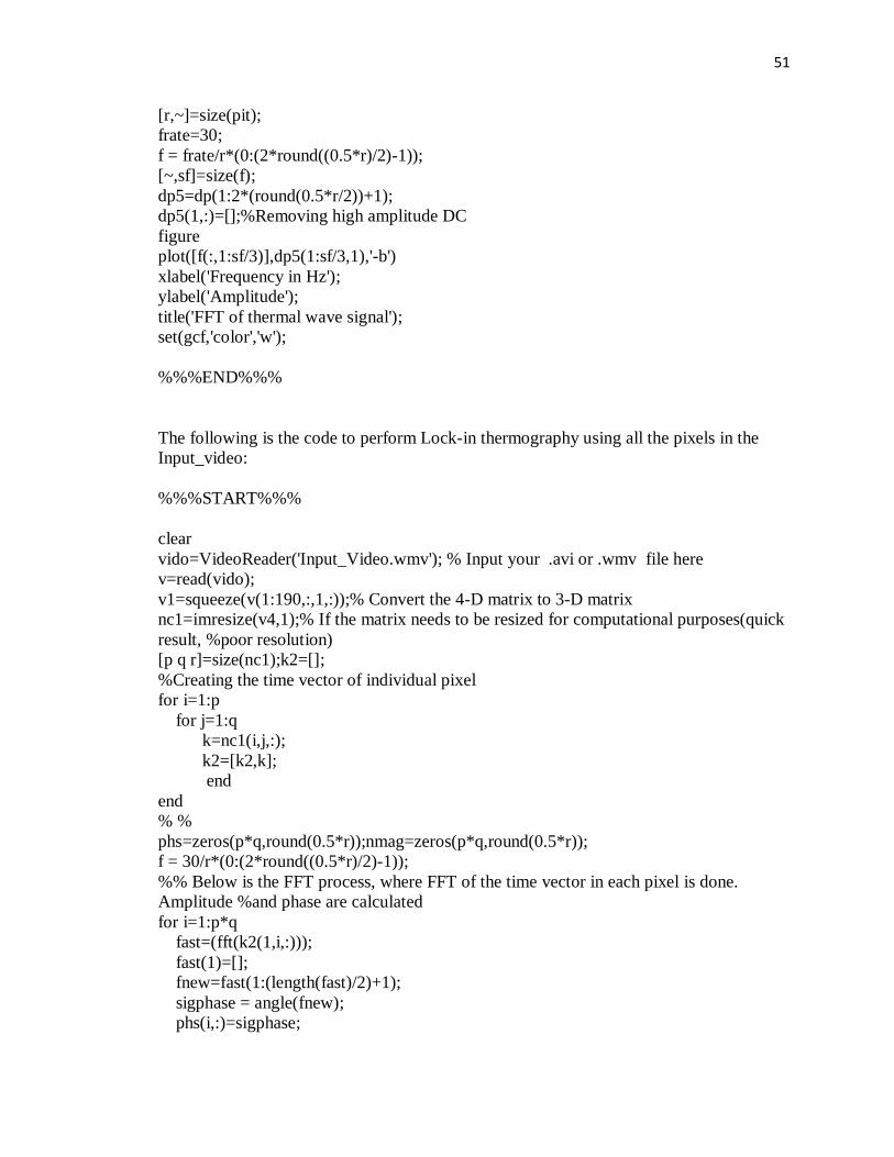
The following is the code to perform Lock-in thermography using all the pixels in the
Input_video:
%%%START%%%
clear
vido=VideoReader('Input_Video.wmv'); % Input your .avi or .wmv file here
v=read(vido);
v1=squeeze(v(1:190,:,1,:));% Convert the 4-D matrix to 3-D matrix
nc1=imresize(v4,1);% If the matrix needs to be resized for computational purposes(quick
result, %poor resolution)
[p q r]=size(nc1);k2=[];
%Creating the time vector of individual pixel
for i=1:p
for j=1:q
k=nc1(i,j,:);
k2=[k2,k];
end
end
% %
phs=zeros(p*q,round(0.5*r));nmag=zeros(p*q,round(0.5*r));
f = 30/r*(0:(2*round((0.5*r)/2)-1));
%% Below is the FFT process, where FFT of the time vector in each pixel is done.
Amplitude %and phase are calculated
for i=1:p*q
fast=(fft(k2(1,i,:)));
fast(1)=[];
fnew=fast(1:(length(fast)/2)+1);
sigphase = angle(fnew);
phs(i,:)=sigphase;
52
mag = abs(fnew);
nmag(i,:)=mag;
end
k2=[];
fz=1; % Plug-in the exact lock-in frequency for accurate results
[~, yin] = min(abs(f - fz));
yi=[1:(p*q)];
nmat1=[];nmat2=[];
magblk=nmag(:,yin);phblk=phs(:,yin);newphase=[];
% For manipulating phase between –π and π
for i=1:p*q
newphase(i,:)=phblk(i,1);
end
% For manipulating phase between 0 to 2π
for i=1:p*q
if phblk(i,1)>0
remin=rem(phblk(i,1),2*pi);
r1=remin;
else
pd2=phblk(i,1)+1000*pi;
r1=rem(pd2,2*pi);
end
newphase(i,:)=r1;
end
%
for i=1:(q):((p*q)-(q-1))
nmat=magblk(i:(i+(q-1)));
nmat1=[nmat1;nmat'];
phmat=newphase(i:(i+(q-1)));
nmat2=[nmat2;phmat'];
end
% % Plots
figure
h1=surf(nmat1);
title('Amplitude')
axis([1 q 1 p])
view(2)
set(gcf,'color','w');
set(gca,'YDir','reverse');
set(gca,'XTick',[]);
set(gca,'YTick',[]);

53
colorbar
grid off
set(h1,'edgecolor','none');
figure
h2=surf(nmat2);
title('Phase')
axis([1 q 1 p])
view(2)
set(gcf,'color','w');
set(gca,'YDir','reverse');
set(gca,'XTick',[]);
set(gca,'YTick',[]);
set(h2,'edgecolor','none');
% caxis([-pi pi]),colorbar % Should be used if the phase is between –π and π
caxis([0 2*pi]),colorbar
grid off
%%%END%%%
Line plot from Amplitude and Phase surface plot
%%%START%%%
figure
[~,ps]=size(nmat1);
% [ps,~]=size(nmat1); Depends on the orientation of the line
mm=(1:ps)./18; %1mm=18pixel(Measure the Field of View)
pnt=30;
[haxes,hline1,hline2] = plotyy(((mm)),nmat1(pnt,:),((mm)),nmat2(pnt,:));
set(hline1, 'LineStyle', '-','Marker', '.','Color',[1 0 0]);
set(hline2, 'LineStyle','-','Marker', '.','Color',[0 0 1]);
set(haxes(1),'YColor', [1 0 0]);
set(haxes(2),'YColor', [0 0 1]);
set(haxes(2),'YLim',[0 2*pi])
set(haxes(2),'YTick',[0 1 2 3 4 5 6])
% set(haxes(2),'YLim',[-pi pi])
% set(haxes(2),'YTick',[-3.14 -2 -1 0 1 2 3.14])
set(gcf,'color','w');
ylabel(haxes(1),'Amplitude of Pixel');
ylabel(haxes(2),'Phase in radians');
xlabel('Distance in mm');
title('Amplitude and Phase')
%%%END%%%
54
MATLAB CODE TO POST-PROCESS THERMAL VIDEOS FROM PULSE
THERMOGRAPHY
The pulse video is read and the pixel of interest is identified.
Then it is plotted.
%%%START%%%
clear;
clc;
% 15 Sec Pulse Thermography
vido=VideoReader('pulse15.wmv'); % Input your .wmv file here
v=read(vido);
v=squeeze(v(:,:,1,:));
v1=v(:,:,:);
[~,~,time]=size(v1);
ti=(1:time)./30;
% Identify the pixel locations in the area of interest and plug in aptly
D1=double(squeeze(v1(43,242,:)));
D3=double(squeeze(v1(45,95,:)));
D4=double(squeeze(v1(168,91,:)));
D2=double(squeeze(v1(162,242,:)));
D5=double(squeeze(v1(107,274,:)));
% D1=double(D1);
% The following smooth fitting function can be used to fit the raw data and obtain the
clean signal
y1 = smooth(ti,D1,0.5,'loess');
y2 = smooth(ti,D2,0.5,'loess');
y3 = smooth(ti,D3,0.5,'loess');
y4 = smooth(ti,D4,0.5,'loess');
y5 = smooth(ti,D5,0.5,'loess');
plot(ti,y1,'-*r',ti,y2,'-*b',ti,y3,'-*g',ti,y4,'-*y',ti,y5,'-*k')
title('15 Sec Pulse Thermography')
legend('2.54mm dia at 0.254mm','1.27mm dia at 0.254mm','2.54mm dia at
0.635mm','1.27mm dia at 0.635mm','Normal Sample')
xlabel('Time in Seconds');
ylabel('Signal between 0 and 255');
set(gcf,'color','w');
%%%END%%%

55
GIF MOVIE GENERATION FROM AMPLITUDE AND PHASE RESULT
This program uses the amplitude and phase data generated from the lock-in program
%%%START%%%
time=1:0.033:5; % Useful to control the time and time intreval
[~,tm]=size(time);
omega=2*pi*fz;
for i=1:tm
shot=nmat1.*cos((nmat2)+omega*time(i));
h3=surf(shot);
set(gcf,'color','w');
set(gca,'ZLim',[-30000 30000]);
caxis([-30000 30000]);colorbar;
set(gca,'YDir','reverse');
% view(2) % (Turn ON if 2-D view is required)
grid off
axis off
camlight;
lighting phong
set(gca, 'XTick', [], 'YTick',[]);
set(h3,'edgecolor','none');
mov(i) = getframe;
[Inx,cmap]=rgb2ind(mov(i).cdata,256);
if i==1
imwrite(Inx,cmap,'output.gif','gif','DelayTime',0.3,'LoopCount',Inf)
else
imwrite(Inx,cmap,'output.gif','gif','WriteMode','append','DelayTime',0.3)
end
end
%%%END%%%

56
BIBLIOGRAPHY
1. Avdelidis, N. and D.P. Almond, Transient thermography as a through skin
imaging technique for aircraft assembly: modelling and experimental results.
Infrared physics & technology, 2004. 45(2): p. 103-114.
2. Ducar, R.J. Pulsed thermographic inspection and application in commercial
aircraft repair. in AeroSense'99. 1999. International Society for Optics and
Photonics.
3. Hellier, C. and C. Hellier, Handbook of nondestructive evaluation. Vol. 10. 2001:
McGraw-Hill New York.
4. Avdelidis, N., B. Hawtin, and D. Almond, Transient thermography in the
assessment of defects of aircraft composites. NDT & E International, 2003. 36(6):
p. 433-439.
5. Genest, M., et al., Pulsed thermography for non-destructive evaluation and
damage growth monitoring of bonded repairs. Composite Structures, 2009. 88(1):
p. 112-120.
6. Huth, S., et al., Localization of gate oxide integrity defects in silicon metal-oxide-
semiconductor structures with lock-in IR thermography. Journal of Applied
Physics, 2000. 88(7): p. 4000-4003.
7. Liu, W. and B. Yang, Thermography techniques for integrated circuits and
semiconductor devices. Sensor Review, 2007. 27(4): p. 298-309.
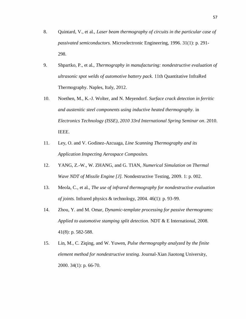
57
8. Quintard, V., et al., Laser beam thermography of circuits in the particular case of
passivated semiconductors. Microelectronic Engineering, 1996. 31(1): p. 291-
298.
9. Shpartko, P., et al., Thermography in manufacturing: nondestructive evaluation of
ultrasonic spot welds of automotive battery pack. 11th Quantitative InfraRed
Thermography. Naples, Italy, 2012.
10. Noethen, M., K.-J. Wolter, and N. Meyendorf. Surface crack detection in ferritic
and austenitic steel components using inductive heated thermography. in
Electronics Technology (ISSE), 2010 33rd International Spring Seminar on. 2010.
IEEE.
11. Ley, O. and V. Godinez-Azcuaga, Line Scanning Thermography and its
Application Inspecting Aerospace Composites.
12. YANG, Z.-W., W. ZHANG, and G. TIAN, Numerical Simulation on Thermal
Wave NDT of Missile Engine [J]. Nondestructive Testing, 2009. 1: p. 002.
13. Meola, C., et al., The use of infrared thermography for nondestructive evaluation
of joints. Infrared physics & technology, 2004. 46(1): p. 93-99.
14. Zhou, Y. and M. Omar, Dynamic-template processing for passive thermograms:
Applied to automotive stamping split detection. NDT & E International, 2008.
41(8): p. 582-588.
15. Lin, M., C. Ziqing, and W. Yuwen, Pulse thermography analyzed by the finite
element method for nondestructive testing. Journal-Xian Jiaotong University,
2000. 34(1): p. 66-70.
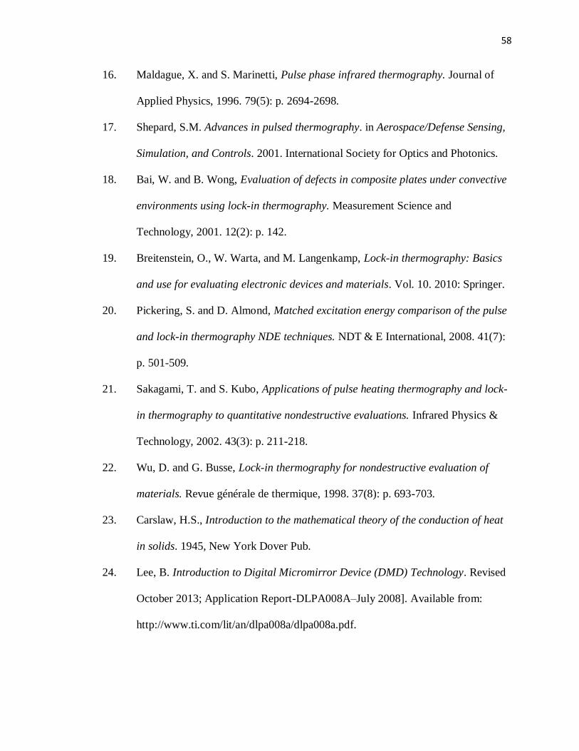
58
16. Maldague, X. and S. Marinetti, Pulse phase infrared thermography. Journal of
Applied Physics, 1996. 79(5): p. 2694-2698.
17. Shepard, S.M. Advances in pulsed thermography. in Aerospace/Defense Sensing,
Simulation, and Controls. 2001. International Society for Optics and Photonics.
18. Bai, W. and B. Wong, Evaluation of defects in composite plates under convective
environments using lock-in thermography. Measurement Science and
Technology, 2001. 12(2): p. 142.
19. Breitenstein, O., W. Warta, and M. Langenkamp, Lock-in thermography: Basics
and use for evaluating electronic devices and materials. Vol. 10. 2010: Springer.
20. Pickering, S. and D. Almond, Matched excitation energy comparison of the pulse
and lock-in thermography NDE techniques. NDT & E International, 2008. 41(7):
p. 501-509.
21. Sakagami, T. and S. Kubo, Applications of pulse heating thermography and lock-
in thermography to quantitative nondestructive evaluations. Infrared Physics &
Technology, 2002. 43(3): p. 211-218.
22. Wu, D. and G. Busse, Lock-in thermography for nondestructive evaluation of
materials. Revue générale de thermique, 1998. 37(8): p. 693-703.
23. Carslaw, H.S., Introduction to the mathematical theory of the conduction of heat
in solids. 1945, New York Dover Pub.
24. Lee, B. Introduction to Digital Micromirror Device (DMD) Technology. Revised
October 2013; Application Report-DLPA008A–July 2008]. Available from:
http://www.ti.com/lit/an/dlpa008a/dlpa008a.pdf.

59
25. Architecture of the Texas Instruments Digital Micromirror Device (DMD). [cited
2015; Available from: http://compliantmechanisms.byu.edu/content/introduction-
microelectromechanical-systems-mems.
26. Instruments, T., DLP 0.55 XGA Chipset.
27. Jackson, J.D. Visual Analysis of a Texas Instruments Digital Micromirror Device.
Available from:
http://www.optics.rochester.edu/workgroups/cml/opt307/spr05/john/.
28. Chatterjee, K., et al., A comparison of the pulsed, lock-in and frequency
modulated thermography nondestructive evaluation techniques. NDT & E
International, 2011. 44(7): p. 655-667.
29. Tuli, S. and R. Mulaveesala, Defect detection by pulse compression in frequency
modulated thermal wave imaging. Quantitative InfraRed Thermography Journal,
2005. 2(1): p. 41-54.
30. Li, T., D.P. Almond, and D.A.S. Rees, Crack imaging by scanning pulsed laser
spot thermography. NDT & E International, 2011. 44(2): p. 216-225.
31. Pech-May, N., et al., Vertical cracks characterization using lock-in
thermography: I infinite cracks. Measurement Science and Technology, 2014.
25(11): p. 115601.
32. Kreyszig, E., Advanced engineering mathematics. 1988: John Wiley & Sons.
33. Structured-light_3D_scanner. 2008 17:54, 18 March 2008 [cited 2015; Available
from: http://en.wikipedia.org/wiki/Structured-light_3D_scanner.

60
VITA
Arvindvivek Ravichandran was born in Chennai, India. He was awarded
Bachelors in Mechanical Engineering from Government College of Technology –
Coimbatore under Anna University in 2008.
He has been working for four years as an engineer in Fuel Cell development and
applications. He worked in Automotive Industry and National Lab in India. He enrolled
in MS in Mechanical Engineering in Fall 2012 and has been awarded Teaching and
Research Assistantship. He has been handling sections of Experimental Methods in
Aerospace Engineering and Introduction to Design as Teaching Assistant. He was
working in Thermal Radiation Laboratory as Research Assistant. He won Third Place in
Student Infra-red Imaging Competition by DRS Technologies among the 27 teams from
nationwide. He graduated with Masters in Mechanical Engineering in May 2015.