spatial data analysis 1

Spatial Data Analysis 1/2

Johan Blomme | Leenstraat 11 | 8340 Damme

[email protected]

Introduction

• Many research questions require analysis of complex patterns of interrelated social, behavioral, economic and environmental phenomena. In addressing these questions, it is increasingly argued that both spatial thinking and spatial analytical perspectives have an important role to play. Indeed, research on social stratification and inequality, health, mortality and fertility and many other issues depends on the collection and analysis of individual and context-level data.

• The geospatial and methodological development environment has changed in the last few years. The volume, sources and forms of available geospatial data are growing rapidly. The flow of information from a host of sensors has grown exponentially in recent years to the point that many observations can be geo-referenced. Data storage and handling (e.g. cloud computing) change what, how and when we collect data on individuals and their environments.

Introduction 3

• In a world where information is increasingly seen through geographic filters, the importance of spatial thinking is addressed. More and more instances show that space and place are important elements and stress the leverage of place-based politics. For example, conventional approaches in health research underestimate the contribution of place to disease risk. Several studies reinforce the view how neighborhood context is an important condition of human well being. Place emerges as an important contextual framework for considering a number of critical societal issues. Place as a social context is deeply connected to larger patterns of social advantage and disadvantage.

Introduction 4

• Since the mid 1990s, there is a renewed interest in the much earlier tradition of spatial demography that focuses on areal aggregates as units of analysis. Trends in technology during the 1980s and 1990s brought sophistication to the world of spacial demography. Factors contributing were :

– U.S. Census Bureau’s TIGER files ;

– extensive natural resource, crime and epidemiological databases ;

– powerful GIS software for integrating and mapping spatial data ;

– computing hardware platforms.

• These factors altered the way in which spatial demography research was carried out. Other trends that emerged were :

– the role of regression analysis in spatial demography ;

– the special nature of spatial data that requires modification to the standard regression model ;

– the need for attention both to global as well as local diagnostic tools ;

– the use of exploratory spacial data analysis (ESDA) ;

– the role of geographically weighted regrssion for exploring spatial variation.

Introduction 5

• When analyzing spatial data from a large number of units (e.g. counties), it is the natural inclination of researchers to move from simple descriptive analysis to begin asking questions as : How might these data be modeled ? How well can we account for variability in attribute values among geographic units ?

• To answer these questions, analysts turned to multivariate regression modeling, the common workhorse methodology in the social sciences. However, the application of the standard regression approach to data tied to spatial units brings spacial complications because “spatial is special”. Attention has been drawn to the fact that spatial data require special analytic approaches.

Introduction 6

• Two properties are particularly important in the analysis of spatial data. The first, spatial dependence, refers to the tendency for spatial data to exhibit spatial autocorrelation. For most social phenomena mapped in space, local proximity usually results in value similarity. High values tend to be located near other high values, while low values tend to be located near other low values, thus exhibiting positive spatial autocorrelation. Less often, high values may tend to be co-located with low values (or vice versa), as islands of dissimilarity (negative spatial autocorrelation).

• In either case, the units of analysis in spacial demography likely fail a key assumption of classical statistics : independence among observations. With respect to statistical analysis that presumes such independence (e.g. standard regression analysis), positive autocorrelation means that the spatially autocorrelated observations bring less information to the model estimation process than would the same number of independent observations. The greater the extent of spatial autocorrelation, the more severe is the information loss.

Introduction 7

• A quick explanation for the presence of spatial autocorrelation can be found in the oft-cited “first law of geography” enunciated by Tobler in 1970 : Everything is related to everything, but near things are more related than distant things” (Tobler, 1970 : 36). Tobler’s first law is somewhat unsatisfying because it doesn’t tell us why this phenomenon arises in practice. The answer to this question can only be approximated with models of the spatial process and the analysts’s theory about the process.

• The second concept refers to spacial heterogeneity, the tendency for phenomena distributed in many spaces to be statistically nonstationary (a lack of stability across space of one or more attribute values). Spacial heterogeneity confounds attempts to generalize because results of an analysis of a limited area will change when the boundaries of the area are shifted.

• One of the more recent and fascinating developments in the design of local statistics is the theoretical background and associated software to explore how regression parameters and regression model performance vary across a study region.

Introduction 8

• Geographically weighted regression (GWR) is similar to a global regression model in that the familiar constant, regression coefficients and error term are all present within the regression specification. There are two ways in which GWR differs from standard (global) regression. First is the fact that a separate regression is carried out at each location (observation) using only the other observations that lie within a user-specified distance from that location. Second, the regression specification includes a statistical device which weights the attributes of nearby geographical units more highly than it does the attributes of distant geographical units. The result is a set of local regression parameters for each geographical unit. The regression is thus localized.

• A GWR approach to regression analysis is a highly useful exploratory device for understanding parameter heterogeneity in one’s data. The output of GWR enables the researcher to examine and map local parameter estimates and local regression diagnostics, thereby enabling assessment of the utility of the model for various positions of the larger study region.

Introduction 9

Spatial Data Analysis with

• The development of specialized software for spatial data analysis has seen rapid growth since the late 1980s.

• A substantial collection of spacial data analysis software is available, ranging from niche programs and commercial statistical and GIS packages to open source software environments such as R, Java and Python.

• GeoDa, for example, is the result of the effort to facilitate spatial data analysis. The main objective of the software is to provide the user with a path starting with simple mapping and geovisualization moving to spatial autocorrelation analysis and ending up with spatial regression.

2

1. Manipulating Spatial Data

Manipulating Spatial Data

4

Creating point shape files from .dbf-file Manipulating Spatial Data

5

Tools → Shape → Points to polygon

Creating Thiessen polygons as shape files

Thiessen polygons are created as a polygon shape file derived from a point shape file. Each Thiessen polygon encloses the original points in such a way that all points in a polygon are closer to the enclosed point than any other point. This corresponds to the notion of geographic market area.

Thiessen polygons allow the computation of contiguity based spatial weights for point data, using the boundaries of the polygons to establish contiguity.

Area and perimeter calculations are only supported for projected coordinates (Euclidean distance). For point shape files in unprojected latitude and longitude, the results will not be correct.


6

Computing spatially lagged variables

Spatially lagged variables are weighted averages of the values for neighboring locations, as specified by a spatial weights matrix.

The changes and additions made to a table only reside in memory and are not permanent. In order To make them permanent, the table must be saved to a new file : File → Save as → Shapefile name to save as This results in three files to be saved, with file extensions .shp, .shx and .dbf.


7

2. Mapping and Exploratory Data Analysis

Mapping and EDA

8

Univariate EDA

9

Univariate EDA

10

resource deprivation index (1970) Hinge value of 1.5 = 1.5 times the interquartile range to define outliers Univariate EDA

11

sort on variable to find outliers

Univariate EDA

12

Univariate EDA

13

Multivariate EDA

Homicide data for counties around St Louis

Quintile map homicide rate Quintile map resource deprivation

14

Multivariate EDA

scatterplot

parallel coordinate plot (PCP)

15

Multivariate EDA

Linking and brushing

16

Multivariate EDA Analyzing changes over time :

17

Multivariate EDA

Cartogram crime rate

Cartogram Gini inequality

18

Ohio counties, total lung cancer deaths for White females, 1968

selecting a rate variable from the data set (reveals the problem of variance instability)

both the event and the population at risk are specified and the rate is calculated on the fly

Rate Smoothing

19

A commonly used notion in public health analysis is the concept of a standardized mortality rate (SMR), or, the ratio of the observed moratlity rate to a national (or regional) standard. GeoDa implements this in the form of an excess risk map. The excess rate is the ratio of the observed rate to the average rate computed for all the data. Note that this average is not the average of the county rates (instead, it is calculated as the ratio of the total sum of all events over the total sum of all populations at risk).

risk is higher than state average

risk is lower than state average

Rate Smoothing

20

saved to the table (right click on previous map)

no difference between rescaled raw rates and raw rates

Rate Smoothing

21

a new outlier is added

Empirical Bayes consists of computing a weighted average between the raw rate for each county and the state average, with weights proportional to the underlying population at risk. Small conties will tend to have their rates adjusted considerably, whereas for larger counties the rates will barely change.

Rate Smoothing

22

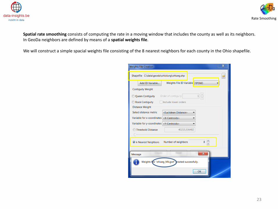
Spatial rate smoothing consists of computing the rate in a moving window that includes the county as well as its neighbors. In GeoDa neighbors are defined by means of a spatial weights file. We will construct a simple spacial weights file consisting of the 8 nearest neighbors for each county in the Ohio shapefile.

Rate Smoothing

23

A spatially smooted box map emphasizes broad regional patterns. Note how there are no more outliers.

Rate Smoothing

24

3. Spatial autocorrelation

Spatial Autocorrelation

25

• Spatial autocorrelation is a measure of spacial dependency that quantifies the degree of spatial clustering or dispersion in the values of a variable measured across a set of locations.

• There are two basic types of spatial autocorrelation statistics : global measures identify whether the values of a variable exhibit a significant overall pattern of regional clustering, whereas local measures identify the location of significant high and low value clusters.


26

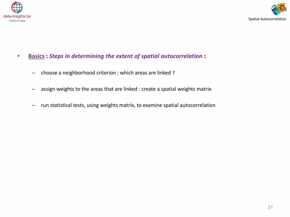
• Basics : Steps in determining the extent of spatial autocorrelation :

– choose a neighborhood criterion : which areas are linked ?

– assign weights to the areas that are linked : create a spatial weights matrix

– run statistical tests, using weights matrix, to examine spatial autocorrelation


27

• Spatial autocorrelation measures the correlation of a variable with itself through space. Spacial autocorrelation can be positive or negative. Positive spatial autocorrelation occurs when similar values occur near one another. Negative spatial autocorrelation occurs when dissimilar values occur near one another.

• Spatial weights are essential for the computation of spacial autocorrelation statistics.

• Spatial weights can be based on contiguity from polygon boundary files or calculated from the distance between points.


28

rook contiguity

queen contiguity

1st order higher order

CONTIGUITYBASED

WEIGHTS .GAL-file

uses only common boundaries to define neighbors

uses all common points (denser connectedness structure)

removes redundancies and circularities in the weights construction

Contiguity Based Weights

polygon shape files

29

flag, number of observations, name of polygon shape file, name of the key variable

Rooks Contiguity

30

Rooks Contiguity

31

Queen Contiguity

32

Comparison of connectedness structure for rook and queen contiguity

Contiguity Based Weights

ROOKS

QUEEN

33

Rooks Contiguity Higher Order Contiguity

34

Pure 2nd order Rooks Contiguity

Higher Order Contiguity

35

Cumulative 2nd order Rooks Contiguity


36


locations with 5 first Order rook neighbors

37

threshold distance

K-nearest neighbors

1st order higher order

DISTANCE BASED

WEIGHTS .GWT-file

GeoDa calculates the minimum distance required to assure that each observation has at least one neighbor

Spacial weights based on distance threshold can lead to a very unbalenced connectedness structure (esp. In the case when spacial units have very different areas, with small areas having many neighbors while larger ones may have only a few). A commonly used alternative consists of considering the k-nearest neighbors.

point or polygon shape files

Distance_Based Weights

38

In contrast to contiguity weights, distance-based spatial weights can be calculated for both point shape files as well as polygon shape files. For polygon files, if no coordinate variables are specified, the polygon centroids will be used as the basis for distance calculation. When polygon shape files are used, maps must be projected (e.g. UTM) for proper computation of centroids. For unprojected maps, the resulting centroids will only approximate.

the minimum distance required to ensure that each location has at least one neighbor

if the points are in latitude and longitude, select the <Arc Distance> option


39

Connectivity for distance-based weights

distance between neighbor pairs

The distribution has a much broader range compared to contiguity-based weights. Some points are clustered while other are far apart. The minimum threshold needed to avoid islands may be too large for many or most locations in the data set. In such cases, care is needed in the specification of the distance threshold, and the use of K-nearest weights may be more appropriate.


40

Spatially Lagged Variables

Spatially lagged variables are an essential part of the computation of spatial autocorrelation tests and the specification of spatial regression models. GeoDa computes these variables on the fly, but in some instances it is useful to calculate spatially lagged variables explicitly. We will calculate a spatially lagged variable for the variable HH_INC (census tract median household income) in the Sacramento file. The first thing we do is open the spatial weights file we created. Then we create a new field that is added to the table.

The value of the spatially lagged variable “W_HH_INC” for this location is the mean of its neighbors

41

Spatially Lagged Variables

42

• Global spatial autocorrelation is handled in GeoDa by means of Moran’s I spatial autocorrelation statistic and its visualization in the form of a scatterplot.

• Global spatial autocorrelation requires a spatial weights file and a variable must be specified.

• Spatial autocorrelation analysis is implemented in its traditional univariate form as well in a bivariate form.

Global Spatial Autocorrelation

43

Moran’s I for Columbus data (variable = crime ; spacial weights file = rooks-based contiguity file)


44

(1) (2)

(3) (4)

negative autocorrelation

positive autocorrelation


45

Moran’s I

reference distribution calculated for spatially random layouts with the same data as observed (none of the simulated values is larger than the observed 0.52)


46

Moran’s I = 0.479487


47

the slope of the regression line changes as specific locations (in this case 1 location) are excluded from the calculation


48

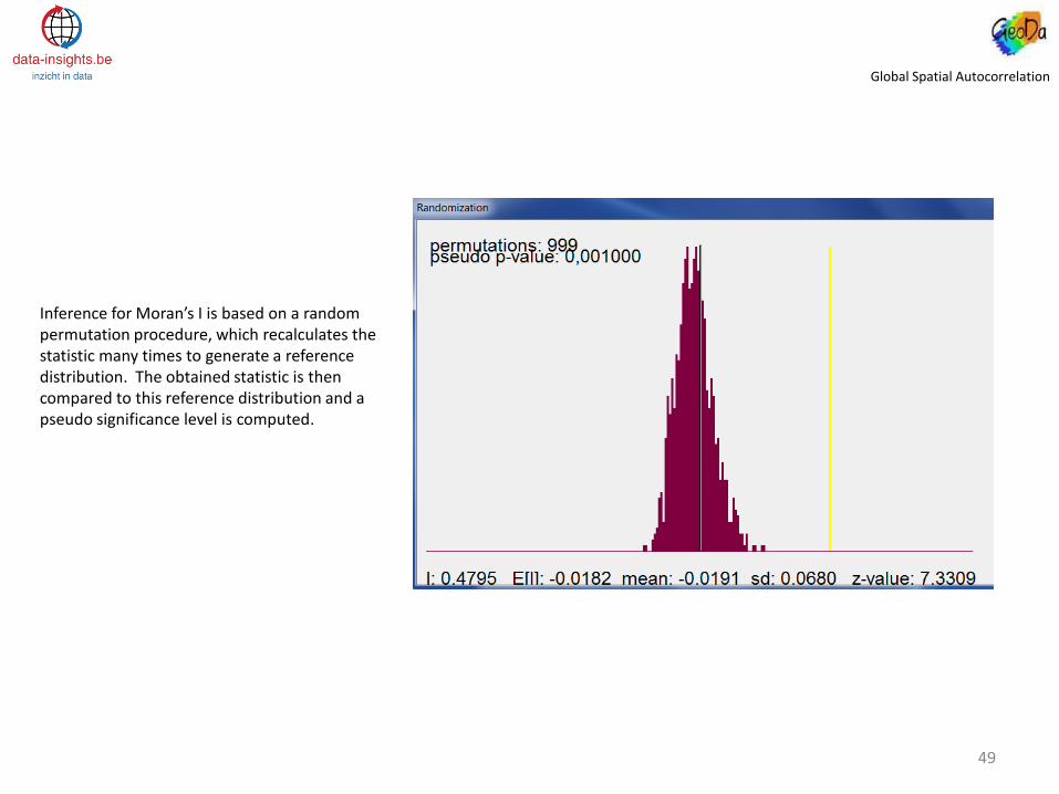
Inference for Moran’s I is based on a random permutation procedure, which recalculates the statistic many times to generate a reference distribution. The obtained statistic is then compared to this reference distribution and a pseudo significance level is computed.


49

A c

ou

nty

’s s

pat

ial l

ag is

a w

eigh

ed a

vera

ge o

f t

he

reso

urc

e d

epri

vati

on

of

its

nei

ghb

ori

ng

loca

litie

s.


50

• Global measures : global spatial autocorrelation (Moran’s I) : a single value which applies to the entire data set (the same pattern or process occurs over the entire geographical area ; and average for the entire area).

• Local measures : local spatial autocorrelation (Lisa) : a value calculated for each observation unit (different patterns of processes may occur in different parts of the region ; a unique number for each location).

Local Spatial Autocorrelation

51

• Local spatial autocorrelation is based on local Moran LISA statistics. This yields a measure of spatial autocorrelation for each individual location.

• Both univariate and multivariate LISA are included in GeoDa.

• The input needed for local spatial autocorrelation is the same as for global spatial autocorrelation.


52

the significance map shows the locations with significant local Moran statistics


the high-high and low-low locations (positive local spatial autocorrelation) are typically referred to as spatial clusters, while the low-high and high-low are termed spatial outliers (while outliers are single locations by definition, this is not the case for clusters)

53


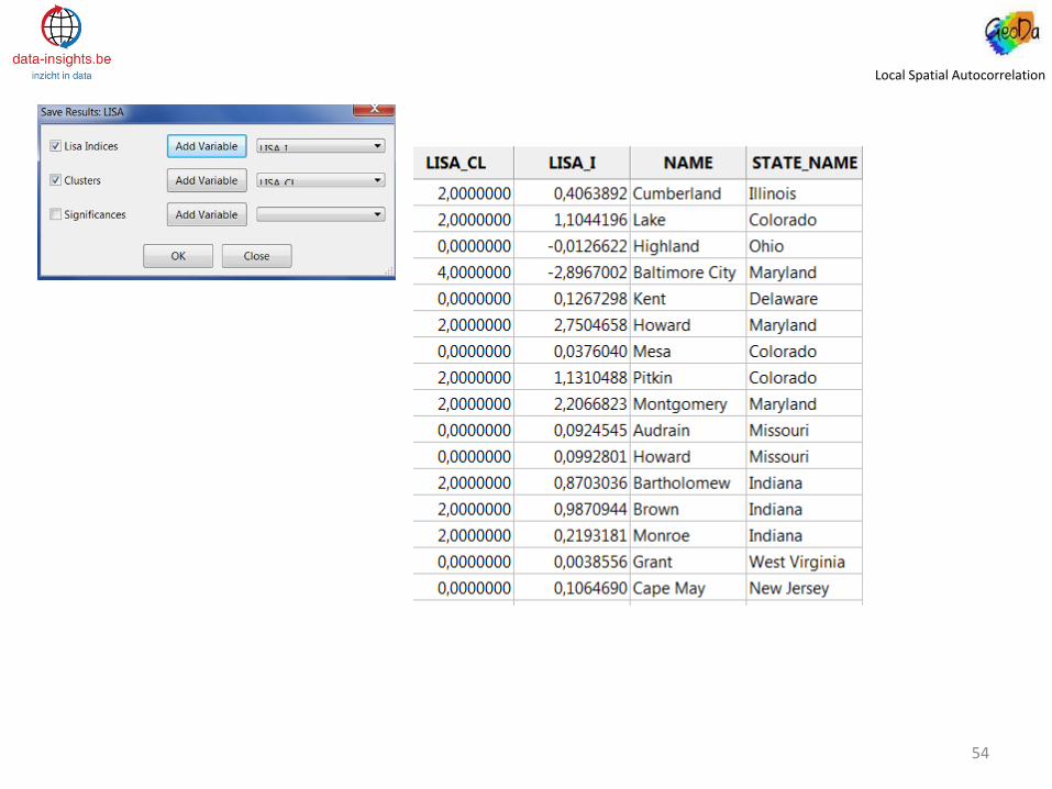
54

The result for univariate LISA is a special chloropleth map showing those locations with a significant local Moran statistic (depending on the significance level). In the map blow, the significance map is shown for the CRIME variable in the Columbus Data set, using rook contiguity.


55

The result of the cluster map is a special choropleth map showing those locations with a significant local Moran statistic Classified by type of spatial correlation : bright red for the high-high association and bright blue for low-low. The high-high and low-low locations suggest clustering of similar values, while the high-low and low-high locations Indicate spatial outliers.


56

It is strongly recommended that sensitivity analysis be carried out before interpreting results of LISA maps as “significant” clusters. The randomization option provides a way to address numerical stability of the results. The significance filter is designed to assess how conclusions depend on the chosen significance level.


57

LISA maps after applying a significance filter.


58


When Moran’s I statistic is calculated for rates or proportions, the underlying assumption of stationarity may be violated by the instrinsic instability of rates. The latter follows when the population at risk (the base) varies considerably across observations. The variance instavility mat lead to spurious inferences for Moran’s I. To correct for this, GeoDa implements the Empirical Bayes (EB) standardization. This is implemented for both the global (Moran scatter plot) and local spatial autocorrelation statistics. To illustrate this, we will use the Scottish lip cancer data set and associated weights file to compare the results of calculating Moran’s I based on the non-standardized rates with the results of the EB standardization.

59

The value for Moran’s I of 0.527 differs somewhat from the statistic for the unstandardized rates (0.479). More important is to assess whether or not inference is affected. The resulting permulation distribution still suggests a highly significant statistic.


60

• Practice : Spatial patterns of rural poverty : An exploratory analysis in the São Fransisco River Bassin, Brazil (Nove Economia_Belo_Horizonte_21 (1), 45-66_janeiro-abril de 2011).

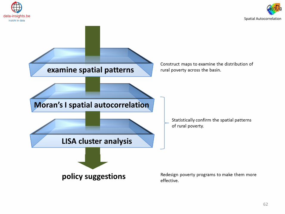
This study uses recently released municipio-level data on rural poverty in Brazil to identify and analyze spatial patterns of rural poverty in the SFRB.

Moran’s I statistics are generated and used to test for spatial autocorrelation, and to prepare cluster maps that locate rural poverty “hot spots” and “cold spots”.

The results indicate that poverty reduction in the SFRB should take into account the spatial distribution of poverty. Not only is poverty in the SFRB clustered spatially, but the bulk of the bassin’s poor resides in municipios that comprise the poverty “hot spots” the study identifies. These clusters did not correspond to state-level boundaries, so scope may exist for geographically refocusing poverty reduction efforts to make them more efficient.


61


62


63

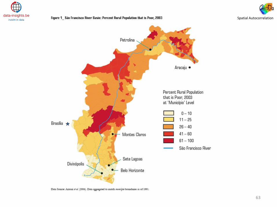
• Information on spatial patterns of rural poverty in the SFRB may shed light on the importance of location as a causal factor per se. Municipios may be more likely to have high (or low) rural poverty rates depending on where they are located geographically :

– one obvious reason is the stock of natural resources (natural resources are not evely distributed across space) : for farm activities, for example, good soils and easy access to water may improve agricultural conditions, productivity and income ;

– job and income providers such as firms and service-oriented businesses tend to concentrate in space in order to benefit from large markets (economies of scale) and the availability of specialized skilled labor.


64

• The value of Moran’s I is equal to 0.72, which suggests a strong positive spatial autocorrelation of rural poverty. This number suggests that for the SFRB, there are more locations wich high (low) rural poverty rates surrounded by locations with high (low) rural poverty rates than would be the case if poverty were distributed randomly.

• The value of Moran’s I also suggests that poverty in the SRFB is spatially distributed in clusters and also suggests that poverty in neighboring areas increases the likelihood of poverty in its neighbors. However, the value of Moran’s I does not tell us where rural poverty clusters might be, but rather suggests that the spatial pattern of poverty is not random (there is more similarity in poverty (or the absence of it) than would be expected if the pattern were random).

• Making use of EB-standardization to reduce variance instability, delivers a coefficient of 0.83 compared to the initial calculation of Moran’s I. This indicates that the correlation between rural poverty rates in location i and neighboring locations is stronger when rates are standardized. Hence, increasing the precision with which rural poverty is measured will likely increase the spatial correlation among rural poverty rates in the SFRB.


65

• Although a Moran I of 0.83 strongly shows that the spatial distribution of rural poverty is not random, it does not locate poverty clusters.

• To locate “hot spots” and “cold spots”, local indicators of spatial autocorrelation must be used (LISA). LISA provides location-specific information and estimates the extent of spatial autocorrelation between the value of a given variable (rural poverty) in a particular location and the values of the same variable in locations around it. This makes it possible to identify spatial clusters of rural poverty.

• 3 clusters of rural poverty in the SFRB are detected by LISA. Clusters 1 and 2 are rural poverty “hot spots” and correspond to positive and high-high spatial autocorrelation, indicating spatial clusters of locations with above-average rural poverty rates. Cluster 3 is a “cold spot” and also corresponds to a positive, but low-low spatial autocorrelation, indicating a cluster of locations with below -average rural poverty rates.


66


67

• As mentioned before, the clusters of rural poverty may be attributable to several reasons. But further analysis is required to determine the causes of spatial patterns of rural poverty in the SFRB. Multivariate regression analysis that takes into account the variables that may explain poverty is the appropriate approach to the analysis of the spacial determinants of patterns of rural poverty in the SFRB.

• The results of this study suggest that poverty reduction policies in the SFRB should take into account the spatial distribution of poverty. The analysis suggests that location as a causal factor per se is important and locations are indeed more likely to have high (or low) rural poverty rates depending in where they are located in the basin. This may be due to obvious reasons such as stock of natural resources, soil quality, access to water, etc.

• More importantly, the analysis shows that poverty in one location is affected by (or affects) poverty in neighboring locations. That is, there are spillovers, either positive or negative externalities that make locations more or less likely to get out of poverty. These spillovers may be associated with the concentration (or lack of concentration) of firms, technology and knowledge. These results set the stage for identifying factors that influence rural poverty in the SFRB, factors that may themselves be spatially correlated.


68

4. Spatial regression

Spatial Regression

69

• When moving from simple descriptive analyses to data modeling, analysts turn to multivariate regression modeling to account for variability in attribute values among geographic units by identifying other covariates of the attribute of interest.

• Attributes of spatially referenced data generally violate at least one of the assumptions underlying the standard regression model, which necessitates both caution regarding these violations and attention to methods designed to correct for them.

Spatial Regression

70

• Spatial variation : spatial heterogeneity versus spatial dependence

• When undertaking initial EDA of spatial data, it is worthwhile to develop a sense of the spatial distribution

of the attribute values. By mapping the distributions of variables across space, a distinction can be made between two types of spatial dependence.

• Spatial heterogeneity : large-scale regional differentiation (among attribute values) is an important component of spatial variation. Spacial heterogeneity is the lack of stability across space of one or more attribute values. Heterogeneity gives recognition to the common observation that values of a variable are not the same across space.

• Spatial heterogeneity follows from the intrinsic uniqueness of each location. Spacial heterogeneity is consistent with the description of how places are particular moments of intersecting social relations. The unique combination of social forces together in one place may produce effects which would not happen otherwise. These social forces include nonmaterial forces (e.g. cultural and/or historical processes) that cannot easily or always be quantified, yet these forces shape otherwise measurable social relationships. The spacial regime approach permits the analyst to move beyond geography per se, by focusing on social, economic and demographic factors - or, combined , sociological factors – that comprise the context of place. This approach is intended to enable the analyst to address the “so what” question : what is it about a place that distinguishes it from other places ?

Spatial Regression

71

• Spatial dependence refers to small-scale spatial effects that manifest a lack of independence among observations (spatial clustering). The assumption is that dependence among the observations derives from spatial interaction among the units of analysis which can be defended theoretically and which can be statistically captured by a spatially lagged “neighborhood” effect.

• Two forms of spacial models are commonly used to improve regressions on spatially correlated data :

– The spacial lag model : if two locations are adjacent, the value of the dependent variable of the first locations can be influenced by the value of the dependent variable of the other. This means that there is a contagion or dispersion effect, represented best by a spatial lag model.

– The spacial error model : if the error residuals of locations are influenced by one another, this means that the phenomenon under study is not analysed at the correct geographical level, or that there might be an unobserved variable correlated with the spatial structure of the data. This would imply a clustering effect and this has to be studied by a spatial error model.

• A spatial lag model is appropriate if neighboring locations influence one another ; the spatial error model documents that locations geographically cluster but for an unknown reason.

Spatial Regression

72

Spatial distribution of population change among Great Plains Counties, 1990-2000 Source : P.R. Voss, K.J. Curtis White & R.B. Hammer : Explorations in spatial demography, in W.A. Kandel & D.L. Brown, Population change and rural society, Springer, 2006, pp. 407-429)

spatial hereogeneity across counties and spacial dependence (clustering)

Moran scatterplot of population change

Spatial Regression

73

• A model with spatial lags is able to borrow information from neighborhood observations because of the spatial autocorrelation among the units of analysis. The units of analysis likely fail a formal statistical test of randomness and thus fail to meet a key assumption of classical statistics : independence among observations. With respect to statistical techniques that presume such independence (e.g. standard regression analysis), positive autocorrelation means that the spatially autocorrelated observations bring less information to the model estimation process than would the same number of independent observations.

• A carefully selected variable can account for spatial heterogeneity in the data and might boost the explanatory value of the model and largely remove the large-scale spatial process, but spatial autocorrelation would persist if a spatial dependence process were also indicated. There would remain in the data a more complicated, interactive spatial relationship among neighbors that suggests the requirement of some type of autoregressive term in the regression specification.

Spatial Regression

74

• The aim of the researcher is to specify and estimate a model that reasonably accounts for or incorporates spatial effects present in the data. These effects can be modeled as spatial heteregeneity and spatial dependence. When first examining a spatial relationship, the reseacher must ask whether the association appears to be a reaction to some geophysical, cultural, social or economic force that works to create spatial patterning (spatial heterogeneity), or an interaction, indicative of spatial dependence.

• If the association is merely a reaction to some general force, then a modeling strategy with a standard regression structure may be appropriate.

• If, on the other hand, the association is an interaction suggesting some type of formal dependency among units, then a modeling strategy with a spatial dependent covariance structure is the way to proceed. In this instance, heterogeneity likely will not fully remove the spatial effects within the data. An alternative is needed – a spatially oriented approach that formally incorporates a spatially lagged dependent variable or spatially lagged error term.

Spatial Regression

75

• Spatial dependency modeling : example 1

• The shapefile newyork.shp is the map of Manhattan in New York City with Census 2000 data* . These are socioeconomic attributes for 297 Census tracts. It includes the following variables:

POLYID Polygon ID STATE State FIPS COUNTY County FIPS TRACT Census Tract ID sctrct00 FIPSID hvalue Median housing value t0_pop Total population pctnhw Percent non-Hispanic white persons pctnhb Percent non-Hispanic black persons pcthsp Percent Hispanic persons pctasn Percent Asian persons t0p_own Percent homeowners t0p_coll Percent college educated t0p_prf Percent of people employed in professional/managerial occupations t0p_uemp Percent of people unemployed t0p_for Percent foreign born persons t0p_rec Percent recent immigrants t0_minc Median household income t0p_poor Percent total population below poverty * Source : http://www.s4.brown.edu/S4/Training/Modul2/GeoDa3FINAL.pdf

Spatial Regression

76

• Before starting a regression, create a weights file :

Spatial Regression

77

• In this example, we will predict neighborhood homeownership with several indicators :

Spatial Regression

78

insignificant effects

Spatial Regression

79

Test of multicollinearity of the model : one should be alarmed when the condition number is greater than 20.

Jarque-Bara test is used to examine the normality of the distribution of the errors. The low probability of the test score suggests non- normal distribution of the error term.

The low probabilities of the three tests point to the existence of heteroscedasticity. Error variance can be affected by spatial dependence in the data.

Moran’s I suggests spatial autocorrelation of the residuals.

Both tests of the lag and error are significant, indicating presence of spatial dependence. The robust test help us understand what type of spatial dependence may be at work. The robust measure for error is still significant, but the robust lag test becomes insignificant, which means that when the lagged dependent variable is present the error dependence disappears.

Spatial Regression

80

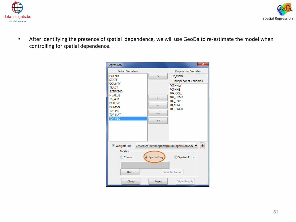
• After identifying the presence of spatial dependence, we will use GeoDa to re-estimate the model when controlling for spatial dependence.

Spatial Regression

81

Spatial Regression

The spatial lag term of homeownership (W_TOP_OWN) appears as an additional indicator. It has a positive effect and is highly significant. As a result, the model fit is improved (higher R-square).

Coefficient Rho reflects the spatial dependence in the sample data, measuring the average influence on observations by their neighboring observations.

Although the introduction of the spacial lag term improved the model fit , it didn’t make the spacial effects go away.

cfr. R2= 0.495 with OLS regression

82

• Now let’s review the results for the spatial error model.

Spatial Regression

83

Coefficient of spatially correlated errors is positive. The model fit is improved (higher R2).

Heteroscedasticity remais significant. Also, spatial error stays significant. Although allowing the error terms to be spatially correlated improved the model fit, it didn’t make the spatial effects go away.

Spatial Regression

84

• Comparing the spatial lag and spatial error models, we can see that both models yield improvement to the original OLS model. Therefore, controlling spatial dependence improves model performance.

• Now the question is which of the two models is better ? To some extent, this is an open question. The general advice is first to look for a theoretical basis to inform your choice. When it is not so clear theoretically, you can compare the model performance parameters : the R-squared and log likelihood. In this example, the spatial error model has greater R-squared and log likelihood values. That provides a statistical basis to adopt this solution.

Spatial Regression

85

Spatial Regression

86

• Spatial dependency modeling : example 2

• Analysis of poverty in the U.S. *

Source : http://csde.washington.edu/services/gis/workshops/SPREG.html

Spatial Regression

87

Spatial Regression

88

violation of regression assumptions

Spatial Regression

89

Spatial Regression

90

Spatial Regression

91

spatial error model

Model R2 Log Likelihood

OLS 0,780 2323,69

Spatial Lag 0,822 2457,37

Spatial Error 0,847 2504,64

Spatial Regression

92

The spatial error form results in a substantial reduction of spatial autocorrelation.

Spatial Regression

93