spatial data analysis - wamis. · pdf file152 spatial data analysis indeed, gis provides a...

SPATIAL DATA ANALYSIS

P.L.N. RajuGeoinformatics DivisionIndian Institute of Remote Sensing, Dehra Dun

Abstract : Spatial analysis is the vital part of GIS. Spatial analysis in GIS involvesthree types of operations- attribute query (also known as non-spatial), spatial queryand generation of new data sets from the original databases. Various spatial analysismethods viz. single/multiplayer operations/overlay; spatial modeling; geometricmodeling; point pattern analysis; network analysis; surface analysis; raster/grid

analysis etc. are discussed in detail in this paper.

INTRODUCTION

Geographic analysis allows us to study and understand the real worldprocesses by developing and applying manipulation, analysis criteria andmodels and to carryout integrated modeling. These criteria illuminateunderlying trends in geographic data, making new information available. AGIS enhances this process by providing tools, which can be combined inmeaningful sequence to reveal new or previously unidentified relationshipswithin or between data sets, thus increasing better understanding of real world.The results of geographic analysis can be commercial in the form of maps,reports or both. Integration involves bringing together diverse information froma variety of sources and analysis of multi-parameter data to provide answersand solutions to defined problems.

Spatial analysis is the vital part of GIS. It can be done in two ways. Oneis the vector-based and the other is raster-based analysis. Since the advent ofGIS in the 1980s, many government agencies have invested heavily in GISinstallations, including the purchase of hardware and software and theconstruction of mammoth databases. Two fundamental functions of GIS havebeen widely realized: generation of maps and generation of tabular reports.

Satellite Remote Sensing and GIS Applications in Agricultural Meteorologypp. 151-174

152 Spatial Data Analysis

Indeed, GIS provides a very effective tool for generating maps and statisticalreports from a database. However, GIS functionality far exceeds the purposesof mapping and report compilation. In addition to the basic functions relatedto automated cartography and data base management systems, the mostimportant uses of GIS are spatial analysis capabilities. As spatial informationis organized in a GIS, it should be able to answer complex questions regardingspace.

Making maps alone does not justify the high cost of building a GIS. Thesame maps may be produced using a simpler cartographic package. Likewise,if the purpose is to generate tabular output, then a simpler databasemanagement system or a statistical package may be a more efficient solution.It is spatial analysis that requires the logical connections between attributedata and map features, and the operational procedures built on the spatialrelationships among map features. These capabilities make GIS a much morepowerful and cost-effective tool than automated cartographic packages,statistical packages, or data base management systems. Indeed, functionsrequired for performing spatial analyses that are not available in eithercartographic packages or data base management systems are commonlyimplemented in GIS.

USING GIS FOR SPATIAL ANALYSIS

Spatial analysis in GIS involves three types of operations: Attribute Query-also known as non-spatial (or spatial) query, Spatial Query and Generation ofnew data sets from the original database (Bwozough, 1987). The scope of spatialanalysis ranges from a simple query about the spatial phenomenon tocomplicated combinations of attribute queries, spatial queries, and alterationsof original data.

Attribute Query: Requires the processing of attribute data exclusive of spatialinformation. In other words, it’s a process of selecting information by askinglogical questions.

Example: From a database of a city parcel map where every parcel is listedwith a land use code, a simple attribute query may require the identificationof all parcels for a specific land use type. Such a query can be handled throughthe table without referencing the parcel map (Fig. 1). Because no spatialinformation is required to answer this question, the query is considered anattribute query. In this example, the entries in the attribute table that haveland use codes identical to the specified type are identified.

P.L.N. Raju 153

Spatial Query: Involves selecting features based on location or spatialrelationships, which requires processing of spatial information. For instance aquestion may be raised about parcels within one mile of the freeway and eachparcel. In this case, the answer can be obtained either from a hardcopy mapor by using a GIS with the required geographic information (Fig. 2).

Parcel Size Value Land UseNo.

102 7,500 200,000 Commercial

103 7,500 160,000 Residential

104 9,000 250,000 Commercial

105 6,600 125,000 Residential

A sample parcel map Attribute table of the sample parcel map

Figure 1: Listing of Parcel No. and value with land use = ‘commercial’ is an attribute query.Identification of all parcels within 100-m distance is a spatial query

Parcels for rezoning

Parcels for notification

Figure 2: Land owners within a specified distance from the parcel to be rezoned identifiedthrough spatial query

Example: Let us take one spatial query example where a request is submittedfor rezoning, all owners whose land is within a certain distance of all parcelsthat may be rezoned must be notified for public hearing. A spatial query isrequired to identify all parcels within the specified distance. This process cannotbe accomplished without spatial information. In other words, the attributetable of the database alone does not provide sufficient information for solvingproblems that involve location.


While basic spatial analysis involves some attribute queries and spatialqueries, complicated analysis typically require a series of GIS operationsincluding multiple attribute and spatial queries, alteration of original data,and generation of new data sets. The methods for structuring and organizingsuch operations are a major concern in spatial analysis. An effective spatialanalysis is one in which the best available methods are appropriately employedfor different types of attribute queries, spatial queries, and data alteration. Thedesign of the analysis depends on the purpose of study.

GIS Usage in Spatial Analysis

GIS can interrogate geographic features and retrieve associated attributeinformation, called identification. It can generate new set of maps by queryand analysis. It also evolves new information by spatial operations. Here aredescribed some analytical procedures applied with a GIS. GIS operationalprocedure and analytical tasks that are particularly useful for spatial analysisinclude:

Single layer operations

Multi layer operations/ Topological overlay

Spatial modeling

Geometric modeling

Calculating the distance between geographic features

Calculating area, length and perimeter

Geometric buffers.

Point pattern analysis

Network analysis

Surface analysis

Raster/Grid analysis

Fuzzy Spatial Analysis

Geostatistical Tools for Spatial Analysis

Single layer operations are procedures, which correspond to queries andalterations of data that operate on a single data layer.

P.L.N. Raju 155

Example: Creating a buffer zone around all streets of a road map is a singlelayer operation as shown in the Figure 3.

Figure 3: Buffer zones extended from streets

Streets

Buffer zones

Multi layer operations: are useful for manipulation of spatial data on multipledata layers. Figure 4 depicts the overlay of two input data layers representingsoil map and a land use map respectively. The overlay of these two layersproduces the new map of different combinations of soil and land use.

Figure 4: The overlay of two data layers creates a map of combined polygons

Topological overlays: These are multi layer operations, which allow combiningfeatures from different layers to form a new map and give new informationand features that were not present in the individual maps. This topic will bediscussed in detail in section of vector-based analysis.


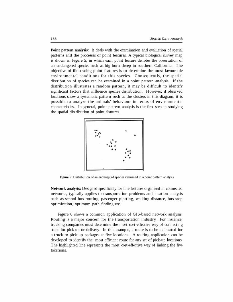
Point pattern analysis: It deals with the examination and evaluation of spatialpatterns and the processes of point features. A typical biological survey mapis shown in Figure 5, in which each point feature denotes the observation ofan endangered species such as big horn sheep in southern California. Theobjective of illustrating point features is to determine the most favourableenvironmental conditions for this species. Consequently, the spatialdistribution of species can be examined in a point pattern analysis. If thedistribution illustrates a random pattern, it may be difficult to identifysignificant factors that influence species distribution. However, if observedlocations show a systematic pattern such as the clusters in this diagram, it ispossible to analyze the animals’ behaviour in terms of environmentalcharacteristics. In general, point pattern analysis is the first step in studyingthe spatial distribution of point features.

Figure 5: Distribution of an endangered species examined in a point pattern analysis

Network analysis: Designed specifically for line features organized in connectednetworks, typically applies to transportation problems and location analysissuch as school bus routing, passenger plotting, walking distance, bus stopoptimization, optimum path finding etc.

Figure 6 shows a common application of GIS-based network analysis.Routing is a major concern for the transportation industry. For instance,trucking companies must determine the most cost-effective way of connectingstops for pick-up or delivery. In this example, a route is to be delineated fora truck to pick up packages at five locations. A routing application can bedeveloped to identify the most efficient route for any set of pick-up locations.The highlighted line represents the most cost-effective way of linking the fivelocations.

P.L.N. Raju 157

Figure 6: The most cost effective route links five point locations on the street map

Surface analysis deals with the spatial distribution of surface information interms of a three-dimensional structure.

The distribution of any spatial phenomenon can be displayed in a three-dimensional perspective diagram for visual examination. A surface mayrepresent the distribution of a variety of phenomena, such as population, crime,market potential, and topography, among many others. The perspectivediagram in Figure 7 represents topography of the terrain, generated fromdigital elevation model (DEM) through a series of GIS-based operations insurface analysis.

Figure 7: Perspective diagram representing topography of the terrain derived from a surface analysis


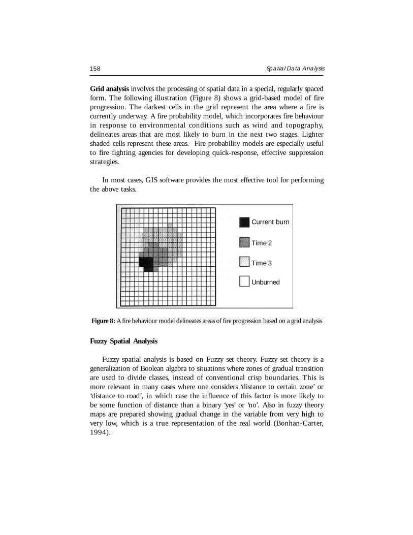
Grid analysis involves the processing of spatial data in a special, regularly spacedform. The following illustration (Figure 8) shows a grid-based model of fireprogression. The darkest cells in the grid represent the area where a fire iscurrently underway. A fire probability model, which incorporates fire behaviourin response to environmental conditions such as wind and topography,delineates areas that are most likely to burn in the next two stages. Lightershaded cells represent these areas. Fire probability models are especially usefulto fire fighting agencies for developing quick-response, effective suppressionstrategies.

In most cases, GIS software provides the most effective tool for performingthe above tasks.

Figure 8: A fire behaviour model delineates areas of fire progression based on a grid analysis

Fuzzy Spatial Analysis

Fuzzy spatial analysis is based on Fuzzy set theory. Fuzzy set theory is ageneralization of Boolean algebra to situations where zones of gradual transitionare used to divide classes, instead of conventional crisp boundaries. This ismore relevant in many cases where one considers ‘distance to certain zone’ or‘distance to road’, in which case the influence of this factor is more likely tobe some function of distance than a binary ‘yes’ or ‘no’. Also in fuzzy theorymaps are prepared showing gradual change in the variable from very high tovery low, which is a true representation of the real world (Bonhan-Carter,1994).

Current burn

Time 2

Time 3

Unburned

P.L.N. Raju 159

As stated above, the conventional crisp sets allow only binary membershipfunction (i.e. true or false), whereas a fuzzy set is a class that admits thepossibility of partial membership, so fuzzy sets are generalization of crisp setsto situations where the class membership or class boundaries are not, or cannotbe, sharply defined.

Applications

Data integration using fuzzy operators using standard rules of fuzzy algebraone can combine various thematic data layers, represented by respectivemembership values (Chung and Fabbri, 1993).

Example: In a grid cell/pixel if a particular litho-unit occurs in combinationwith a thrust/fault, its membership value should be much higher comparedwith individual membership values of litho-unit or thrust/fault. This issignificant as the effect is expected to be “increasive” in our presentconsideration and it can be calculated by fuzzy algebraic sum. Similarly, ifthe presence of two or a set of parameters results in “decreasive” effect, it canbe calculated by fuzzy algebraic product. Besides this, fuzzy algebra offersvarious other methods to combine different data sets for landslide hazardzonation map preparation. To combine number of exploration data sets, fivesuch operators exist, namely the fuzzy AND, the fuzzy OR, fuzzy algebraicproduct, fuzzy algebraic sum and fuzzy gamma operator.

Fuzzy logic can also be used to handle mapping errors or uncertainty, i.e.errors associated with clear demarcation of boundaries and also errors presentin the area where limited ground truth exists in studies such as landslidehazard zonation. The above two kinds of errors are almost inherent to theprocess of data collection from different sources including remote sensing.

GEOSTATISTICAL TOOLS FOR SPATIAL ANALYSIS

Geostatistics studies spatial variability of regionalized variables: Variables thathave an attribute value and a location in a two or three-dimensional space.Tools to characterize the spatial variability are:

Spatial Autocorrelation Function and

Variogram.


A variogram is calculated from the variance of pairs of points at differentseparation. For several distance classes or lags, all point pairs are identifiedwhich matches that separation and the variance is calculated. Repeating thisprocess for various distance classes yields a variogram. These functions can beused to measure spatial variability of point data but also of maps or images.

Spatial Auto-correlation of Point Data

The statistical analysis referred to as spatial auto-correlation, examines thecorrelation of a random process with itself in space. Many variables that havediscrete values measured at several specific geographic positions (i.e., individualobservations can be approximated by dimensionless points) can be consideredrandom processes and can thus be analyzed using spatial auto-correlationanalysis. Examples of such phenomena are: Total amount of rainfall, toxicelement concentration, grain size, elevation at triangulated points, etc.

The spatial auto-correlation function, shown in a graph is referred to asspatial auto-correlogram, showing the correlation between a series of points ora map and itself for different shifts in space or time. It visualizes the spatialvariability of the phenomena under study. In general, large numbers of pairsof points that are close to each other on average have a lower variance (i.e.,are better correlated), than pairs of points at larger separation. The auto-correlogram quantifies this relationship and allows gaining insight into thespatial behaviour of the phenomenon under study.

Point Interpolation

A point interpolation performs an interpolation on randomly distributedpoint values and returns regularly distributed point values. The variousinterpolation methods are: Voronoi Tesselation, moving average, trend surfaceand moving surface.

Example: Nearest Neighbor (Voronoi Tessellation)-In this method thevalue, identifier, or class name of the nearest point is assigned to the pixels. Itoffers a quick way to obtain a Thiessen map from point data (Figure 9).

P.L.N. Raju 161

VECTOR BASED SPATIAL DATA ANALYSIS

In this section the basic concept of various vector operations are dealt indetail. There are multi layer operations, which allow combining features fromdifferent layers to form a new map and give new information and features thatwere not present in the individual maps.

Topological overlays: Selective overlay of polygons, lines and points enablesthe users to generate a map containing features and attributes of interest,extracted from different themes or layers. Overlay operations can be performedon both raster (or grid) and vector maps. In case of raster map calculationtool is used to perform overlay. In topological overlays polygon features of onelayer can be combined with point, line and polygon features of a layer.

Polygon-in-polygon overlay:

Output is polygon coverage.

Coverages are overlaid two at a time.

There is no limit on the number of coverages to be combined.

New File Attribute Table is created having information about each newlycreated feature.

Line-in-polygon overlay:

Output is line coverage with additional attribute.

No polygon boundaries are copied.

New arc-node topology is created.

Figure 9: (a) An input point map, (b) The output map obtained as the result of theinterpolation operation applying the Voronoi Tessellation method

(a) (b)


Point-in-polygon overlay:

Output is point coverage with additional attributes.

No new point features are created.

No polygon boundaries are copied.

Logical Operators: Overlay analysis manipulates spatial data organized indifferent layers to create combined spatial features according to logicalconditions specified in Boolean algebra with the help of logical and conditionaloperators. The logical conditions are specified with operands (data elements)and operators (relationships among data elements).

Note: In vector overlay, arithmetic operations are performed with the help oflogical operators. There is no direct way to it.

Common logical operators include AND, OR, XOR (Exclusive OR), andNOT. Each operation is characterized by specific logical checks of decisioncriteria to determine if a condition is true or false. Table 1 shows the true/false conditions of the most common Boolean operations. In this table, A andB are two operands. One (1) implies a true condition and zero (0) impliesfalse. Thus, if the A condition is true while the B condition is false, then thecombined condition of A and B is false, whereas the combined condition ofA OR B is true.

AND - Common Area/ Intersection / Clipping Operation

OR - Union Or Addition

NOT - (Inverter)

XOR - Minus

Table 1: Truth Table of common Boolean operations

A B A AND B A OR B A NOT B B NOT A A XOR B

0 0 0 0 0 0 0

0 1 0 1 0 1 1

1 0 0 1 1 0 1

1 1 1 1 0 0 0

P.L.N. Raju 163

The most common basic multi layer operations are union, intersection,and identify operations. All three operations merge spatial features on separatedata layers to create new features from the original coverage. The maindifference among these operations is in the way spatial features are selectedfor processing.

Overlay operations

The Figure 10 shows different types of vector overlay operations and givesflexibility for geographic data manipulation and analysis. In polygon overlay,features from two map coverages are geometrically intersected to produce a

Figure 10 : Overlay operations

OPERATION PRIMARY LAYER OPERATION LAYER RESULT

CLIP

ERASE

SPLIT

IDENTITY

UNION

INTERSECT

1 2

3 4

1 2

3 4

1 2

3 4

1 2

3 4

1 2

3 4

1 2

3 4

1 2

3 4

1 2

3 4

12 3

4

67 8

9

2 4

5 8

2 36 7

1 72 4

3 12

3 510 12

3 14

16 9

11

4

2 3

8 116 12

1 46 12

1 6


new set of information. Attributes for these new features are derived from theattributes of both the original coverages, thereby contain new spatial andattribute data relationships.

One of the overlay operation is AND (or INTERSECT) in vector layeroperations, in which two coverages are combined. Only those features in thearea common to both are preserved. Feature attributes from both coveragesare joined in the output coverage.

Input Coverage Intersect Coverage Output Coverage

INPUTCOVERAGE

# ATTRIBUTE

1 A

2 B

3 A

4 C

5 A

6 D

7 A

INTERSECTCOVERAGE

# ATTRIBUTE

1

2 102

3 103

OUTPUT INPUT INTERSECTCOVERAGE COVERAGE COVERAGE

# # ATTRIBUTE # ATTRIBUTE

1 1 A 2 102

2 2 B 2 102

3 3 A 2 102

4 3 A 3 103

5 5 A 3 103

6 4 C 3 103

7 4 C 2 102

8 6 D 3 103

9 7 A 2 102

10 6 D 2 102

P.L.N. Raju 165

RASTER BASED SPATIAL DATA ANALYSIS

Present section discusses operational procedures and quantitative methodsfor the analysis of spatial data in raster format. In raster analysis, geographicunits are regularly spaced, and the location of each unit is referenced by rowand column positions. Because geographic units are of equal size and identicalshape, area adjustment of geographic units is unnecessary and spatialproperties of geographic entities are relatively easy to trace. All cells in a gridhave a positive position reference, following the left-to-right and top-to-bottomdata scan. Every cell in a grid is an individual unit and must be assigned avalue. Depending on the nature of the grid, the value assigned to a cell canbe an integer or a floating point. When data values are not available forparticular cells, they are described as NODATA cells. NODATA cells differfrom cells containing zero in the sense that zero value is considered to be data.

The regularity in the arrangement of geographic units allows for theunderlying spatial relationships to be efficiently formulated. For instance, thedistance between orthogonal neighbors (neighbors on the same row or column)is always a constant whereas the distance between two diagonal units can alsobe computed as a function of that constant. Therefore, the distance betweenany pair of units can be computed from differences in row and columnpositions. Furthermore, directional information is readily available for anypair of origin and destination cells as long as their positions in the grid areknown.

Advantages of using the Raster Format in Spatial Analysis

Efficient processing: Because geographic units are regularly spaced withidentical spatial properties, multiple layer operations can be processed veryefficiently.

Numerous existing sources: Grids are the common format for numeroussources of spatial information including satellite imagery, scanned aerial photos,and digital elevation models, among others. These data sources have beenadopted in many GIS projects and have become the most common sources ofmajor geographic databases.

Different feature types organized in the same layer: For instance, the samegrid may consist of point features, line features, and area features, as long asdifferent features are assigned different values.


Grid Format Disadvantages

Data redundancy: When data elements are organized in a regularly spacedsystem, there is a data point at the location of every grid cell, regardlessof whether the data element is needed or not. Although, severalcompression techniques are available, the advantages of gridded data arelost whenever the gridded data format is altered through compression. Inmost cases, the compressed data cannot be directly processed for analysis.Instead, the compressed raster data must first be decompressed in orderto take advantage of spatial regularity.

Resolution confusion: Gridded data give an unnatural look and unrealisticpresentation unless the resolution is sufficiently high. Conversely, spatialresolution dictates spatial properties. For instance, some spatial statisticsderived from a distribution may be different, if spatial resolution varies,which is the result of the well-known scale problem.

Cell value assignment difficulties: Different methods of cell valueassignment may result in quite different spatial patterns.

Grid Operations used in Map Algebra

Common operations in grid analysis consist of the following functions,which are used in Map Algebra to manipulate grid files. The Map Algebralanguage is a programming language developed to perform cartographicmodeling. Map Algebra performs following four basic operations:

Local functions: that work on every single cell,

Focal functions: that process the data of each cell based on the informationof a specified neighborhood,

Zonal functions: that provide operations that work on each group of cellsof identical values, and

Global functions: that work on a cell based on the data of the entiregrid.

The principal functionality of these operations is described here.

P.L.N. Raju 167

Local Functions

Local functions process a grid on a cell-by-cell basis, that is, each cell isprocessed based solely on its own values, without reference to the values ofother cells. In other words, the output value is a function of the value orvalues of the cell being processed, regardless of the values of surrounding cells.For single layer operations, a typical example is changing the value of eachcell by adding or multiplying a constant. In the following example, the inputgrid contains values ranging from 0 to 4. Blank cells represent NODATAcells. A simple local function multiplies every cell by a constant of 3 (Fig.11). The results are shown in the output grid at the right. When there isno data for a cell, the corresponding cell of the output grid remains a blank.

Figure 11: A local function multiplies each cell in the input grid by 3 to produce the outputgrid

Local functions can also be applied to multiple layers represented bymultiple grids of the same geographic area (Fig. 12).

Figure 12: A local function multiplies the input grid by the multiplier grid to produce theoutput grid

Local functions are not limited to arithmetic computations. Trigonometric,exponential, and logarithmic and logical expressions are all acceptable fordefining local functions.


Focal Functions

Focal functions process cell data depending on the values of neighboringcells. For instance, computing the sum of a specified neighborhood andassigning the sum to the corresponding cell of the output grid is the “focalsum” function (Fig. 13). A 3 x 3 kernel defines neighborhood. For cells closerto the edge where the regular kernel is not available, a reduced kernel is usedand the sum is computed accordingly. For instance, a 2 x 2 kernel adjuststhe upper left corner cell. Thus, the sum of the four values, 2,0,2 and 3 yields7, which becomes the value of this cell in the output grid. The value of thesecond row, second column, is the sum of nine elements, 2, 0, 1, 2, 3, 0, 4,2 and 2, and the sum equals 16.

Figure 13: A Focal sum function sums the values of the specified neighborhood to producethe output grid

Another focal function is the mean of the specified neighborhood, the“focal mean” function. In the following example (Fig. 14), this function yieldsthe mean of the eight adjacent cells and the center cell itself. This is thesmoothing function to obtain the moving average in such a way that the valueof each cell is changed into the average of the specified neighborhood.

Figure 14: A Focal mean function computes the moving average of the specifiedneighborhood to produce the output grid

Other commonly employed focal functions include standard deviation(focal standard deviation), maximum (focal maximum), minimum (focalminimum), and range (focal range).

P.L.N. Raju 169

Zonal Functions

Zonal functions process the data of a grid in such a way that cell of thesame zone are analyzed as a group. A zone consists of a number of cells thatmay or may not be contiguous. A typical zonal function requires two grids –a zone grid, which defines the size, shape and location of each zone, and avalue grid, which is to be processed for analysis. In the zone grid, cells of thesame zone are coded with the same value, while zones are assigned differentzone values.

Figure 15 illustrates an example of the zonal function. The objective ofthis function is to identify the zonal maximum for each zone. In the inputzone grid, there are only three zones with values ranging from 1 to 3. Thezone with a value of 1 has five cells, three at the upper right corner and twoat the lower left corner. The procedure involves finding the maximum valueamong these cells from the value grid.

Typical zonal functions include zonal mean, zonal standard deviation, zonalsum, zonal minimum, zonal maximum, zonal range, and zonal variety. Otherstatistical and geometric properties may also be derived from additional zonalfunctions. For instance, the zonal perimeter function calculates the perimeterof each zone and assigns the returned value to each cell of the zone in theoutput grid.

Global Functions

For global functions, the output value of each cell is a function of theentire grid. As an example, the Euclidean distance function computes thedistance from each cell to the nearest source cell, where source cells are definedin an input grid. In a square grid, the distance between two orthogonalneighbors is equal to the size of a cell, or the distance between the centroidlocations of adjacent cells. Likewise, the distance between two diagonal

Figure 15: A Zonal maximum function identifies the maximum of each zone to producethe output grid


neighbors is equal to the cell size multiplied by the square root of 2. Distancebetween non-adjacent cells can be computed according to their row andcolumn addresses.

In Figure 16, the grid at the left is the source grid in which two clustersof source cells exist. The source cells labeled 1 are the first clusters, and thecell labeled 2 is a single-cell source. The Euclidean distance from any sourcecell is always equal to 0. For any other cell, the output value is the distancefrom its nearest source cell.

In the above example, the measurement of the distance from any cell mustinclude the entire source grid; therefore this analytical procedure is a globalfunction.

Figure 17 provides an example of the cost distance function. The sourcegrid is identical to that in the preceding illustration. However, this time acost grid is employed to weigh travel cost. The value in each cell of the costgrid indicates the cost for traveling through that cell. Thus, the cost fortraveling from the cell located in the first row, second column to its adjacentsource cell to the right is half the cost of traveling through itself plus half thecost of traveling through the neighboring cell.

Figure 16: A Euclidean distance function computes the distance from the nearest sourcecell

Figure 17: Travel cost for each cell is derived from the distance to the nearest source cellweighted by a cost function

P.L.N. Raju 171

Another useful global function is the cost path function, which identifiesthe least cost path from each selected cell to its nearest source cell in terms ofcost distance. These global functions are particularly useful for evaluating theconnectivity of a landscape and the proximity of a cell to any given entities.

SOME IMPORTANT RASTER ANALYSIS OPERATIONS

In this section some of the important raster based analysis are dealt:

Renumbering Areas in a Grid File

Performing a Cost Surface Analysis

Performing an Optimal Path Analysis

Performing a Proximity Search

Area Numbering: Area Numbering assigns a unique attribute value to eacharea in a specified grid file. An area consists of two or more adjacent cells thathave the same cell value or a single cell with no adjacent cell of the same value.To consider a group of cells with the same values beside each other, a cellmust have a cell of the same value on at least one side of it horizontally orvertically (4-connectivity), or on at least one side horizontally, vertically, ordiagonally (8-connectivity). Figure 18 shows a simple example of areanumbering.

Figure 18. Illustrates simple example of Area numbering with a bit map as input. The pixels,which are connected, are assigned the same code. Different results are obtained when onlythe horizontal and vertical neighbors are considered (4-connected) or whether all neighborsare considered (8-connected)

One can renumber all of the areas in a grid, or you can renumber onlythose areas that have one or more specific values. If you renumber all of the


areas, Area Number assigns a value of 1 to the first area located. It then assignsa value of 2 to the second area, and continues this reassignment method untilall of the areas are renumbered. When you renumber areas that contain aspecified value (such as 13), the first such area is assigned the maximum gridvalue plus 1. For example, if the maximum grid value is 25, Area Numberassigns a value of 26 to the first area, a value of 27 to the second area, andcontinues until all of the areas that contain the specified values arerenumbered.

Cost Surface Analysis: Cost Surface generates a grid in which each grid cellrepresents the cost to travel to that grid cell from the nearest of one or morestart locations. The cost of traveling to a given cell is determined from a weightgrid file. Zero Weights option uses attribute values of 0 as the start locations.The By Row/Column option uses the specified row and column location asthe start location.

Optimal Path: Optimal Path lets us analyze a grid file to find the best pathbetween a specified location and the closest start location as used in generatinga cost surface. The computation is based on a cost surface file that you generatewith Cost Surface.

One must specify the start location by row and column. The zeros in theinput cost surface represent one endpoint. The specified start locationrepresents the other endpoint.

Testing the values of neighboring cells for the smallest value generates thepath. When the smallest value is found, the path moves to that location,where it repeats the process to move the next cell. The output is the path ofleast resistance between two points, with the least expensive, but not necessarilythe straightest, line between two endpoints. The output file consists of onlythe output path attribute value, which can be optionally specified, surroundedby void values.

Performing A Proximity Search: Proximity lets you search a grid file for allthe occurrences of a cell value or a feature within either a specified distanceor a specified number of cells from the origin.

You can set both the origin and the target to a single value or a set ofvalues. The number of cells to find can also be limited. For example, if you

P.L.N. Raju 173

specify to find 10 cells, the search stops when 10 occurrences of the cell havebeen found within the specified distance of each origin value. If you do notlimit the number of cells, the search continues until all target values arelocated.

The output grid file has the user-type code and the data-type code of theinput file. The gird-cell values in the output file indicate whether the gridcell corresponds to an origin value, the value searched for and located withinthe specified target, or neither of these.

The origin and target values may be retained as the original values orspecified to be another value.

GRID BASED SPATIAL ANALYSIS

Diffusion modeling and Connectivity analysis can be effectively conducted fromgrid data. Grid analysis is suitable for these types of problems because of thegrid’s regular spatial configuration of geographic units.

Diffusion Modeling: It deals with the process underlying spatial distribution.The constant distance between adjacent units makes it possible to simulatethe progression over geographic units at a consistent rate. Diffusion modelinghas a variety of possible applications, including wildfire management, diseasevector tracking, migration studies, and innovation diffusion research, amongothers.

Connectivity Analysis: Connectivity analysis evaluates inter separation distance,which is difficult to calculate in polygon coverage, but can be obtained muchmore effectively in a grid.

The connectivity of a landscape measures the degree to which surfacefeatures of a certain type are connected. Landscape connectivity is an importantconcern in environmental management. In some cases, effective managementof natural resources requires maximum connectivity of specific features. Forinstance, a sufficiently large area of dense forests must be well connected toprovide a habitat for some endangered species to survive. In such cases, forestmanagement policies must be set to maintain the highest possible level toconnectivity. Connectivity analysis is especially useful for natural resource andenvironmental management.


CONCLUSIONS

GIS is considered as a decision making tool in problem solvingenvironment. Spatial analysis is a vital part of GIS and can be used for manyapplications like site suitability, natural resource monitoring, environmentaldisaster management and many more. Vector, raster based analysis functionsand arithmetic, logical and conditional operations are used based on therecovered derivations.

REFERENCES

Bonhan - Carter, G.F. 1994. Geographic Information Systems for Geoscientists. Love PrintingService Ltd., Ontario, Canada.

Burrough, P.A. 1987. Principles of Geographical Information System for Land Assessment.Oxford : Clardon Press.

Chung, Chang-Jo F. and Fabbri, A.G. 1993. The representation of Geoscience Informationfor data integration. Nonrenewable Resources, Vol. 2, No. 2, Oxford Univ. Press.

spatial data analysis - wamis. · pdf file152 spatial data analysis indeed, gis provides a...

Documents