spatial ecology of coyotes in the denver metropolitan area

1414

Published by Oxford University Press on behalf of the American Society of Mammalogists. This work is written by (a) US Government employee(s) and is in the public domain in the US.

Spatial ecology of coyotes in the Denver metropolitan area: influence of the urban matrix

Sharon a. PoeSSel,* Stewart w. Breck, and eric M. GeSe

Department of Wildland Resources, Utah State University, 5230 Old Main Hill, Logan, UT 84322, USA (SAP)United States Department of Agriculture-Wildlife Services-National Wildlife Research Center, 4101 Laporte Ave., Fort Collins, CO 80521, USA (SWB)United States Department of Agriculture-Wildlife Services-National Wildlife Research Center, Department of Wildland Resources, Utah State University, 5230 Old Main Hill, Logan, UT 84322, USA (EMG)Present address of SAP: U.S. Geological Survey, Forest and Rangeland Ecosystem Science Center, 970 S. Lusk St., Boise, ID 83706, USA

* Correspondent: [email protected]

Urbanization alters landscapes and ecosystem processes that result in negative impacts for many species. However, urbanization also creates novel environments that certain species, including carnivores, are able to exploit. Coyotes (Canis latrans) are 1 example of a species capable of exploiting urban environments throughout North America and, in some cases, becoming involved in human–coyote conflict. As part of a comprehensive study of human–coyote coexistence in the Denver metropolitan area of Colorado, we investigated the spatial ecology of coyotes to determine movement and activity patterns relative to the urban matrix. We examined home-range size, habitat use, and resource selection for 22 coyotes monitored with GPS collars during 2012–2014. Mean (± SD) home-range size of resident coyotes (11.6 ± 11.0 km2) was smaller than ranges of transient coyotes (200.7 ± 232.4 km2). Home-range size did not vary by season or sex, but resident coyotes during the day (7.2 ± 10.5 km2) had smaller home ranges than during the night (11.3 ± 10.8 km2). Coyotes had high percentages of developed lands (44.5 ± 18.9%) within their home ranges, contrary to previous studies of urban coyotes. However, the percentage of coyote locations in natural lands (48.9 ± 22.4%) was higher than in developed lands (20.6 ± 11.7%). Home-range size of residents was not related to either the percentage of developed lands or altered lands within home ranges. Coyotes selected natural lands over developed lands, and they increased activity at night. Although coyotes were able to thrive in home ranges containing large amounts of development, they continued to avoid areas with high human activity by primarily residing in areas with natural land cover. Similar to urban areas throughout the Northern Hemisphere, coyotes in the Denver metropolitan area have become efficiently adapted to a highly developed landscape, reflecting the flexible nature of this opportunistic carnivore.

Key words: Canis latrans, habitat use, home range, human–wildlife conflict, resource selection, urban ecology

Urbanization is altering landscapes worldwide, eliminating habitat for many species but also creating novel environments for species that are able to adapt to the urban matrix (Czech et al. 2000; McKinney 2002). Coyotes (Canis latrans) in North America are supreme generalists and have readily colonized urban landscapes (Gehrt et al. 2009). Coyotes are usually the top wildlife predator in urban areas and positively impact urban ecosystems through predation and competition (Crooks and Soulé 1999; Gehrt and Riley 2010). However, coyotes also are involved in conflicts with urban residents, primarily through attacks on pets and, occasionally, people (Gehrt and

Riley 2010; Poessel et al. 2013). As a result, the coyote has been identified as one of the most controversial carnivore spe-cies in urban areas of North America (Gehrt 2007; Gehrt and Riley 2010).

Coyote spatial and temporal use of urban environments has been studied in only a few North American metropoli-tan areas. These studies of urban coyote ecology have deter-mined coyotes select natural habitat patches within their home ranges and minimize activity near areas of human develop-ment (Quinn 1997; Grinder and Krausman 2001; Gehrt et al. 2009; Gese et al. 2012). Home-range sizes of coyotes in urban

Journal of Mammalogy, 97(5):1414–1427, 2016DOI:10.1093/jmammal/gyw090Published online May 28, 2016

Downloaded from https://academic.oup.com/jmammal/article-abstract/97/5/1414/2219095by Miami University useron 02 March 2018

mailto:[email protected]?subject=

POESSEL ET AL.—SPATIAL ECOLOGY OF URBAN COYOTES 1415

environments may increase as the amount of urbanization within home ranges increases (Riley et al. 2003; Gehrt et al. 2009; Gese et al. 2012), indicating that dense development is less suitable than undeveloped natural areas within a city (Riley et al. 2003). Furthermore, urban coyotes also become more active at night when humans are least active (Quinn 1997; Grinder and Krausman 2001; Riley et al. 2003), and they generally are not attracted to human-associated areas within home ranges (Gehrt et al. 2009).

Habitat use and selection in coyotes may differ between males and females and between residents and transients. Grinder and Krausman (2001) determined female habitat selection was the primary driver of the overall trend in coyote selection of habitat in their study. Poessel et al. (2014) also found that females exhib-ited strong preferences in habitat selection and patch choice, whereas males had no patterns in habitat preferences. Home ranges of resident coyotes may be more associated with natural habitats than those of transients. Gehrt et al. (2009) determined that home ranges of many resident coyotes, but not transients, in their study were almost completely contained within large natu-ral habitat fragments, although natural land cover was nonethe-less the dominant habitat type for both residents and transients.

Our objectives were to estimate home-range size, assess habitat use, and evaluate resource selection for coyotes in the Denver metropolitan area. We hypothesized 1) home ranges of resident coyotes would be smaller than those of transients, 2) coyotes would have large amounts of natural areas within their home ranges, 3) home-range sizes would increase as the percent of developed areas within home ranges increased, 4) coyotes would use developed areas more at night than during the day, and 5) coyotes would select natural habitat over developed areas. Our results will increase understanding of coyote ecology in the Denver metropolitan area, elucidate differences between coyotes in our study area and coyotes in other urban areas, and supple-ment current knowledge of urban coyotes in North America.

Materials and Methods

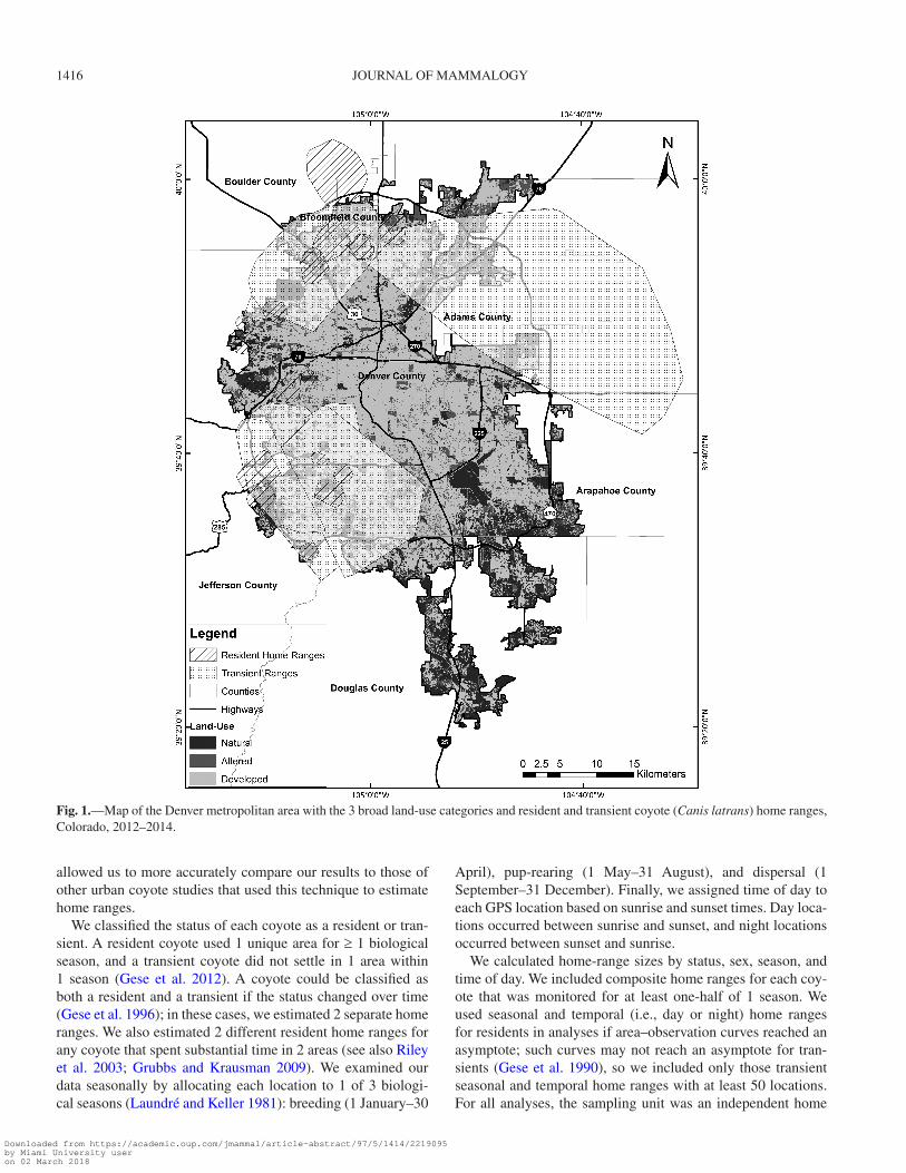
Study area.—We conducted our study in the Denver metro-politan area, which included all or parts of 7 counties (Adams, Arapahoe, Boulder, Broomfield, Denver, Douglas, and Jefferson) and over 35 municipalities in north-central Colorado (Fig. 1). The Denver urban area as defined by the United States Census Bureau spanned approximately 1,760 km2 and had a human population size of almost 2.4 million in 2010 (United States Census Bureau 2012). Monthly temperatures during the study ranged from a mean low of −10°C in December to a mean high of 32°C in July, and average annual precipitation was 43 cm (Weather Underground 2014). The study area consisted of a gradient of urbanization and a variety of land cover types, including agriculture, grasslands, shrublands, and woodlands (Poessel et al. 2013; Magle et al. 2014).

Coyote capture and telemetry.—We captured coyotes with padded foothold traps and snares from April 2012 to May 2013, except during summer months when pups were active. We chose locations throughout the study area where we could gain access and minimize encountering people and pets. For trap-ping, we attached a tranquilizer trap device (TTD) designed to

reduce injuries related to trapping (Sahr and Knowlton 2000). We also attached a trap monitor (Trap-Alert; New Frequency, Inc., Atlanta, Georgia) to the trap, which sent a text message to the researcher’s mobile phone when an animal was captured in the trap, allowing us to arrive at the trap site and process the animal within 1–2 h of capture. Traps were covered dur-ing the day to minimize nontarget captures. We used snares in only 1 location, and these were attached to openings in fences, did not include TTDs or trap monitors, and were checked each morning. Upon capture, we restrained coyotes with a pin stick, muzzled and blind-folded them, and used a rope to hobble their legs. We recorded sex, weight, temperature, morphological measurements, and general body condition, and we estimated age based on tooth wear (Gier 1968). We attached uniquely colored plastic ear tags and fitted each coyote with a GPS radiocollar. Once coyotes had recovered from the tranquilizer (if ingested), they were released at the capture site. Our proce-dures conformed to the guidelines of the American Society of Mammalogists (Sikes et al. 2011), and the Institutional Animal Care and Use Committee at the National Wildlife Research Center (QA-1972) approved trapping and handling protocols.

We used 1 of 3 types of GPS collars: 1) VECTRONIC GPS Plus (VECTRONIC Aerospace GmbH, Berlin, Germany); 2) Lotek GPS 3300S (Lotek Wireless Inc., Newmarket, Ontario, Canada); and 3) Telonics TGW-4400 (Telonics Inc., Mesa, Arizona). We programmed VECTRONIC collars to acquire GPS positions 6 times per day every day and Lotek collars to collect GPS posi-tions 6 times per day 4 days per week for coyotes captured in 2012 and 7 times per day every day for coyotes captured in 2013. Telonics collars were deployed only on coyotes captured at Rocky Mountain Metropolitan Airport in Broomfield, Colorado, and these collars collected GPS locations 6 times per day every day until mid-October 2013, then collected only 1 location every 11 h. For all collars, we concentrated location acquisitions dur-ing nocturnal and crepuscular hours because urban coyotes are generally more active during these times (Grinder and Krausman 2001; Riley et al. 2003; Gehrt et al. 2009; Gese et al. 2012). We downloaded data from collars either remotely from a receiver when the collars were still deployed (VECTRONIC collars) or directly from the collars after they were retrieved (Lotek and Telonics collars). All collars were equipped with automatic release mechanisms; we retrieved collars either when they dropped off or upon death of the animal.

Home-range size.—We estimated home-range size for each coyote by calculating 95% minimum convex polygons (MCPs) using the adehabitatHR package (Calenge 2006) in R (R Core Team 2014). We used MCPs rather than kernel home-range estimators because they included the areas between separate, disjunct polygons often created by kernel estimators (Riley et al. 2003; Gehrt et al. 2009; Riley et al. 2010). These areas were important to include within home ranges so that areas available for use by coyotes would be correctly estimated in resource selection functions. Several of our resident coyotes also exhibited exploratory movements which should not be considered part of the animal’s home range; 95% MCPs are likely to remove these outliers, whereas kernel estimators typi-cally include all clusters of locations. Finally, our use of MCPs


1416 JOURNAL OF MAMMALOGY

allowed us to more accurately compare our results to those of other urban coyote studies that used this technique to estimate home ranges.

We classified the status of each coyote as a resident or tran-sient. A resident coyote used 1 unique area for ≥ 1 biological season, and a transient coyote did not settle in 1 area within 1 season (Gese et al. 2012). A coyote could be classified as both a resident and a transient if the status changed over time (Gese et al. 1996); in these cases, we estimated 2 separate home ranges. We also estimated 2 different resident home ranges for any coyote that spent substantial time in 2 areas (see also Riley et al. 2003; Grubbs and Krausman 2009). We examined our data seasonally by allocating each location to 1 of 3 biologi-cal seasons (Laundré and Keller 1981): breeding (1 January–30

April), pup-rearing (1 May–31 August), and dispersal (1 September–31 December). Finally, we assigned time of day to each GPS location based on sunrise and sunset times. Day loca-tions occurred between sunrise and sunset, and night locations occurred between sunset and sunrise.

We calculated home-range sizes by status, sex, season, and time of day. We included composite home ranges for each coy-ote that was monitored for at least one-half of 1 season. We used seasonal and temporal (i.e., day or night) home ranges for residents in analyses if area–observation curves reached an asymptote; such curves may not reach an asymptote for tran-sients (Gese et al. 1990), so we included only those transient seasonal and temporal home ranges with at least 50 locations. For all analyses, the sampling unit was an independent home

Fig. 1.—Map of the Denver metropolitan area with the 3 broad land-use categories and resident and transient coyote (Canis latrans) home ranges, Colorado, 2012–2014.



range for each individual coyote. We used t-tests to determine differences in composite home-range sizes between residents and transients and between males and females within each status group, and differences in temporal home-range sizes between day and night within each status group. We used anal-ysis of variance to evaluate seasonal differences in home-range sizes by sex for resident coyotes. For each test, we log-trans-formed the home-range size response variable to meet distri-butional assumptions. We conducted all analyses within R (R Core Team 2014), and we considered all statistical tests with P < 0.05 to be statistically significant.

Habitat use.—We report habitat use, in addition to resource selection, to provide descriptive data on the actual use of the landscape by coyotes, regardless of the availability of habitat. Only reporting whether or not coyotes selected a habitat type does not provide information on the animals’ actual use of each habitat type, which could be important information, especially in urban areas where carnivore use of the landscape can be a concern to both residents and land managers (Riley et al. 2010). We examined coyote habitat use within home ranges by analyz-ing 2 variables, land-use and distance to roads. We first obtained land-use data from Landscape Fire and Resource Management Planning Tools (LANDFIRE 2013). We used ArcGIS v.10.0 (ESRI 2010) to condense this data set, in 30-m resolution, into 11 types (Table 1). We further condensed 5 land-use types into a natural lands category, 2 types into an altered lands category, and 4 types into a developed lands category (Table 1). The nat-ural lands category represented coyote use of natural habitat, the altered lands category represented coyote use of nonnatural areas which were likely to be more attractive than developed areas but less attractive than natural habitat (Riley et al. 2003), and the developed lands category represented coyote use of developed landscapes. We then calculated the average percent-age of coyote home ranges in each of the 3 land-use categories. We also assigned a land-use category to each coyote location

and calculated the average percentage of locations in each of the 3 categories. Land-use association can be measured using either of these methods (i.e., percentage of home ranges or per-centage of locations); we used both methods to examine coyote actual use of each land-use type and the amount of each type in coyote home ranges.

We used simple linear regression in R (R Core Team 2014) to determine the relationship between the percentage of urban-ization within a coyote’s home range and home-range size. We conducted 2 regression analyses, 1 with the percentage of developed lands as the explanatory variable and 1 with the per-centage of altered lands as the explanatory variable, with home-range size the dependent variable in both analyses. We included both of these analyses to examine change in the size of a coy-ote’s home range with increasing urbanization, and both devel-oped and altered lands included characteristics of urbanization and human influence. We log-transformed the home-range size response variable to meet distributional assumptions. For these analyses, we only used composite home ranges for resident coyotes.

We further analyzed the natural and developed land-use cat-egories to determine how coyote land-use differed among the 5 natural and 4 developed types. We calculated the average per-centage of coyote home ranges and the average percentage of coyote locations within each of the 5 natural land-use types and each of the 4 developed land-use types. We conducted all land-use analyses for the following coyote groups: all coyotes, by status, by time of day, and by time of day within status.

Next, we calculated the distance of each coyote location to the nearest highway or major road. We obtained road data from the Colorado Department of Transportation. Highways were defined as interstates, United States highways, and state highways. Major roads were defined as public roads classified as arterials (high-capacity urban roads that deliver traffic from collector roads to highways) or collectors (low-to-moderate

Table 1.—Land-use types, categories, and descriptions used to evaluate coyote (Canis latrans) land-use in the Denver metropolitan area, 2012–2014. The percentage of the Denver urban area in each land-use type is also shown.

Land-use type Land-use category Description % of Denver urban area

Forest Natural Dominated by trees (nonriparian) 1.6Shrubland Natural Dominated by shrubs (nonriparian) 6.5Grassland Natural Dominated by herbaceous/nonvascular plants (nonriparian) 5.7Riparian Natural Dominated by water or water-dependent vegetation (i.e., wetlands,

floodplains, swamps, marshes, riparian systems, and open water)4.7

Sparse Natural Barren and sparsely vegetated areas with no dominant life form 0.4Open space Altered Urban vegetated systems (i.e., city parks, golf courses, and cemeteries) 12.9Agriculture Altered Croplands, pasture and hay fields, orchards, and vineyards 6.0Low development Developed Areas with a mixture of constructed materials and vegetation; impervious

surfaces account for 20–49% of the total cover; most commonly include single-family housing units; does not include roads

24.1

Medium development Developed Areas with a mixture of constructed materials and vegetation; impervious surfaces account for 50–79% of the total cover; most commonly include single-family housing units; does not include roads

11.5

High development Developed Highly developed areas where people reside or work in high numbers; impervious surfaces account for 80–100% of the total cover; include apartment complexes, row houses, and commercial/industrial; does not include roads

4.4

Roads Developed All roads 22.2



capacity roads that deliver traffic from local streets to arterial roads). We combined both road types for analysis. We used ArcGIS v.10.0 (ESRI 2010) to calculate the distance from each coyote location to the nearest road, and then averaged these distances for each of the coyote groups included in the land-use analysis.

Resource selection.—We used resource selection function models to investigate use versus availability of the 3 broad land-use categories and distances to roads. We examined 3rd-order selection only, i.e., use versus availability within a coy-ote’s home range (Johnson 1980). We used the lme4 package in R (Bates et al. 2014) to run 3 sets of generalized linear mixed models (GLMMs) using composite, seasonal, and temporal home ranges. We included models for the seasonal and tem-poral home ranges to analyze resource selection by season and time of day; these 2 variables were not available in the models for the composite home ranges. For each model set, we used the coyote locations contained within each 95% MCP home range to represent use, and we generated 5,000 random points within each home range to represent availability. We used a large avail-ability sample to ensure we adequately represented the avail-able landscape and the logistic regression models accurately approximated point process models (Northrup et al. 2013).

All GLMMs included coyote ID as a random effect and sex, status, land-use, and distance to roads as fixed effects. We did not include age because of the lack of a definitive determina-tion of age at time of capture. We rescaled the distance to roads variable by subtracting the mean distance from each value and dividing by 2 times the SD (Gelman 2008). For categorical variables, reference categories were female (sex), resident (sta-tus), and natural (land-use). The seasonal models also included season as a fixed effect, with breeding season as the reference, and the temporal models included time of day as a fixed effect, with day as the reference. For each model set, we first ran a global model with all fixed effects and interactions between sex and land-use, status and land-use, sex and distance to roads, and status and distance to roads. We included additional inter-actions in the seasonal models between season and land-use and season and distance to roads, and we included interactions in the temporal models between time and land-use and time and distance to roads. We then used the MuMIn package in R (Barton 2014) to run all possible model combinations (Doherty et al. 2012) based on the global model in each model set. We used Akaike’s Information Criterion (AIC) to select the best-performing models, based on delta AIC < 6, model weights, and evidence ratios, which indicate the strength of the top model relative to each model in the model set (Burnham and Anderson 2002; Anderson 2008).

Because only 1 model contained 100% of the model weights in each model set (see “Results”), we did not average models and only considered further each top model. We then used the effects package in R (Fox 2003) to calculate the effect displays, i.e., the mean probability of use, for each combination of pre-dictors in the interactions for each top model. We used 95% confidence intervals for each effect to determine significance of contrasts between different predictor combinations. We then

used these results to determine whether coyotes selected roads or certain land-use categories, and whether such selection dif-fered by sex, status, season, or time of day.

results

Capturing and locating coyotes.—We captured and radiocol-lared 32 coyotes (18 males, 14 females). Of these, we were able to retrieve data from the collars of 24 coyotes (14 males, 10 females). Of the 8 coyotes for which we did not retrieve data, 6 coyotes either dispersed from the study area or the collars mal-functioned so we could not receive a signal, 1 coyote was killed by a vehicle and the collar was too damaged to retrieve the data, and 1 coyote had a collar that did not drop off as sched-uled. We had a sufficient number of locations from 22 coyotes (13 males, 9 females) to estimate home-range sizes (mean ± SD = 1,236 ± 712 locations, range = 217–2,449 locations); these coyotes were monitored an average of 316 ± 163 days (range = 57–569 days) between April 2012 and June 2014. Of these 22 coyotes, 7 had Vectronic collars, 13 had Lotek collars, and 2 had Telonics collars.

Home-range size.—We estimated 28 composite coyote home ranges, including 2 home ranges (1 resident and 1 transient) for 4 coyotes (2 males, 2 females) and 2 separate resident home ranges plus 1 transient range for 1 female coyote. Two of the 4 coyotes with 2 home ranges were juveniles whose status switched from resident to transient as they dispersed from their natal home ranges, 1 coyote was a transient when captured who then settled into a resident home range, and 1 coyote was a resi-dent male who lost his mate, dispersed in search of a new mate, then returned to his original home range with his new mate. The female coyote with 3 home ranges dispersed from a resi-dent territory, then eventually settled into a different resident home range. We estimated 54 temporal home ranges (26 day and 28 night) and 65 seasonal home ranges (20 breeding, 21 pup-rearing, and 24 dispersal). Mean (± SD) home-range size of resident coyotes (11.6 ± 11.0 km2) was smaller than transient coyotes (200.7 ± 232.4 km2; t10 = −6.70, P < 0.001). Resident home-range size for males (11.3 ± 4.8 km2) was not different than females (11.9 ± 16.1 km2; t11 = 1.00, P = 0.337), nor was transient range size different between males (288.9 ± 315.5 km2) and females (112.6 ± 75.9 km2; t6 = 1.03, P = 0.342). Home-range size for resident coyotes during the day (7.2 ± 10.5 km2) was smaller than during the night (11.3 ± 10.8 km2; t33 = −2.61, P = 0.014), but home-range size for transient coy-otes was not different between day (202.8 ± 214.2 km2) and night (191.6 ± 228.7 km2; t13 = 0.37, P = 0.716). Seasonal coyote home ranges of residents did not vary by season (F2,48 = 1.54, P = 0.226) or sex (F1,48 = 1.07, P = 0.306).

Habitat use.—Percentages in each land-use category and type are reported for the all-coyote group, unless otherwise indicated; statistical analyses of coyote habitat selection are reported in the “Resource selection” section below. For the land-use analysis using the 3 broad categories, home ranges of each coyote group, except resident coyotes during the day, had the highest mean (± SD) percentages in the developed lands



category (44.5 ± 18.9%), the next highest mean percentages in the natural lands category (32.5 ± 22.9%), and the lowest mean percentages in the altered lands category (23.1 ± 14.6%). Home ranges of resident coyotes during the day had a higher mean percentage of natural lands (40.7 ± 29.7%) than developed lands (34.2 ± 20.9%; Fig. 2). In contrast, the mean percentage of coyote locations in natural lands (48.9 ± 22.4%) was highest for every coyote group, the mean percentage of locations in altered lands (30.5 ± 19.5%) was intermediate for each coyote group, and the mean percentage of locations in developed lands (20.6 ± 11.7%) was lowest for every coyote group (Fig. 2). Each of the 3 land-use categories was included in every coyote’s home range, and each coyote had locations in each category. Home-range size of residents was not related to the percentage of developed lands within home ranges (F1,18 = 0.003, P = 0.959, R2 = 0.0001; Fig. 3a) or the percentage of altered lands within home ranges (F1,18 = 1.042, P = 0.321, R2 = 0.0547; Fig. 3b).

For the natural lands analysis, home ranges of each coyote group, except transients, had the highest mean percentages in riparian (37.9 ± 28.1%) and the lowest mean percentages in sparse (1.6 ± 1.5%). Home ranges generally contained low average per-centages of forest (8.0 ± 9.7%) and intermediate average percent-ages of shrubland (25.3 ± 19.5%) and grassland (27.2 ± 15.0%; Fig. 4). For transient coyotes, the mean percentages of home ranges in riparian (32.5 ± 24.9%) and shrubland (32.6 ± 17.4%) were similar. Likewise, the mean percentage of coyote locations in riparian (41.6 ± 28.7%) was highest, and in sparse (0.7 ± 1.2%) was lowest, for every coyote group except transient coyotes during the night. The mean percentages of coyote locations in forest (12.7 ± 13.9%), shrubland (21.4 ± 19.3%), and grassland (23.7 ± 11.8%) were low to intermediate for each coyote group

(Fig. 4). Transient coyotes in the night had higher mean percent-ages in shrubland (31.4 ± 14.6%) and grassland (33.3 ± 15.5%) than in riparian (26.2 ± 23.7%). One resident coyote had no ripar-ian habitat and 5 coyotes had no sparse habitat within their home ranges. Three coyotes had no locations in forest, 1 coyote had no locations in shrubland, 1 coyote had no locations in riparian, and 8 coyotes had no locations in sparse habitat.

For the developed lands analysis, home ranges of each coyote group had the highest mean percentages in areas of low development (44.1 ± 7.0%), the next highest mean per-centages in roads (35.7 ± 8.0%), the next highest mean per-centages in areas of medium development (17.0 ± 6.2%), and the lowest mean percentages in areas of high development (3.2 ± 3.0%; Fig. 5). Similarly, the mean percentage of coy-ote locations was highest in either areas of low development (47.2 ± 17.0%) or in roads (45.6 ± 19.2%), the next highest in areas of medium development (6.8 ± 5.5%), and lowest in areas of high development (0.4 ± 1.0%), for each coyote group (Fig. 5). Two coyotes had no areas of high development in their home ranges, and 15 coyotes had no locations in areas of high development.

The average (± SD) distance for coyote locations to the nearest road was 364 ± 240 m for all coyotes, 364 ± 193 m for residents, 365 ± 349 m for transients, 392 ± 275 m for day loca-tions, 346 ± 209 m for night locations, 389 ± 233 m for day locations of resident coyotes, 401 ± 380 m for day locations of transient coyotes, 351 ± 177 m for night locations of residents, and 332 ± 288 m for night locations of transients. Three of the 4 coyotes with the largest nearest distances to roads (i.e., farthest from roads) also had the smallest percentages of developed lands within their home ranges.

Fig. 2.—Percentages of coyote (Canis latrans) home ranges and locations during the day and night within each of the 3 broad land-use categories for a) residents and b) transients, Denver, Colorado, 2012–2014.



Resource selection.—In each of the 3 model sets, the fully parameterized global model with all interactions was the top model with 100% of the model weights (Tables 2 and 3). In the composite model, females and males had no differences in their use of all 3 land-use categories (Fig. 6a). Within females and males, both groups used natural and altered lands the same, but used developed lands less than both natural and altered lands (Fig. 6a). Resident coyotes used natural lands more than transients, but use of altered and developed lands was similar between the 2 groups (Fig. 6b). Within residents and tran-sients, both groups used natural and altered lands the same, but used developed lands less than both natural and altered lands (Fig. 6b). Female coyotes (Fig. 6c) and transient coyotes (Fig. 6d) selected roads, with higher probability of use of habi-tat closer to roads. Male coyotes (Fig. 6c) and resident coyotes (Fig. 6d) had no selection for or against roads. For an aver-age coyote (i.e., based on the intercept of the model), variation among individuals ranged from 11% to 60%.

In the seasonal model, we found no seasonal patterns in habitat selection. Coyotes did not use natural, altered, or devel-oped lands any differently among the 3 seasons (Fig. 7a), nor did they have any selection for or against roads within any season (Fig. 7b). Within each season, coyotes used natural and altered lands the same, but used developed lands less than both natural and altered lands (Fig. 7a). Results for females and males were similar to those in the composite model, except females used natural and altered lands more than males, and male coyotes selected against roads, with higher probability of use of habitat farther from roads. Results for residents and transients were similar to those in the composite model, except

Fig. 3.—Linear regression of average home-range sizes for resident coyotes (Canis latrans) on percentage of urbanization within coy-ote home ranges for a) developed land-use and b) altered land-use, Denver, Colorado, 2012–2014.

Fig. 4.—Percentages of coyote (Canis latrans) home ranges and locations during the day and night within each of the 5 natural land-use types (see Table 1) for a) residents and b) transients, Denver, Colorado, 2012–2014.



residents used natural lands more than altered lands. For an average coyote, variation among individuals within the 3 sea-sons ranged from 4% to 32%.

In the temporal model, coyotes used all 3 land-use catego-ries more during the night than in the day (Fig. 7c). During the day, coyotes used natural lands more than both altered and developed lands, and they used developed lands less

than altered lands (Fig. 7c). During the night, coyotes used natural and altered lands the same, but used developed lands less than both natural and altered lands (Fig. 7c). Coyotes selected roads at night, but coyotes during the day had no selection for or against roads (Fig. 7d). Results for females and males, as well as for residents and transients, were simi-lar to those in the composite model. For an average coyote,

Fig. 5.—Percentages of coyote (Canis latrans) home ranges and locations during the day and night within each of the 4 developed land-use types (see Table 1) for a) residents and b) transients, Denver, Colorado, 2012–2014.

Table 2.—Top 2 models in Akaike’s Information Criterion (AIC) model selection in each of 3 model sets used to determine coyote (Canis latrans) habitat selection in the Denver metropolitan area, 2012–2014. Each model set represents resource selection within composite, seasonal, or temporal coyote home ranges. K refers to the number of parameters (including intercept) in a model plus 1 for the error term. The evidence ratio represents the strength of the top model relative to the 2nd model in each model set.

Model K Delta AIC Model weight Evidence ratio

Composite model set: Sex, Status, Land-use, Roads, Sex * Land-use,

Status * Land-use, Sex * Roads, Status * Roads13 0.00 1.0000 —

Sex, Status, Land-use, Roads, Sex * Land-use, Status * Land-use, Sex * Roads

12 27.22 0.0000 813,960.97

Seasonal model set: Sex, Status, Season, Land-use, Roads, Sex *

Land-use, Status * Land-use, Season * Land-use, Sex * Roads, Status * Roads, Season * Roads

22 0.00 0.9975 —

Sex, Status, Season, Land-use, Roads, Sex * Land-use, Status * Land-use, Season * Land-

use, Sex * Roads, Status * Roads

20 12.42 0.0020 498.83

Temporal model set: Sex, Status, Time, Land-use, Roads, Sex *

Land-use, Status * Land-use, Time * Land-use, Sex * Roads, Status * Roads, Time * Roads

18 0.00 1.0000 —

Sex, Status, Time, Land-use, Roads, Sex * Land-use, Status * Land-use, Time * Land-use,

Sex * Roads, Status * Roads

17 21.14 0.0000 39,000.35



variation among individuals within the 2 temporal periods ranged from 6% to 26%.

discussion

Home-range size.—We found considerable individual varia-tion in home-range sizes of both resident and transient coyotes in the Denver metropolitan area. Among residents, females had high variation, with the largest home-range size for a female (53.6 km2) being more than 2.5 times greater than the largest home-range size for a male (19.9 km2). Home-range

sizes of resident coyotes in our study were no different than those reported for residents in a rural area in southeastern Colorado (mean size 11.3 km2—Gese et al. 1988), contrary to the trend for smaller home ranges in other urban landscapes (Gehrt and Riley 2010). Resident home ranges were smaller than those of transients, consistent with other coyote studies in both urban areas (Gehrt et al. 2009; Gese et al. 2012) and rural areas (Gese et al. 1988). Resident coyotes also had smaller home ranges during the day than at night, similar to findings by Gese et al. (1990) and Smith et al. (1981) in rural areas. Coyotes near Seattle, Washington (Quinn 1997), Los Angeles,

Table 3.—Beta coefficients from the top model in each of 3 model sets used to determine coyote (Canis latrans) habitat selection in the Denver metropolitan area, 2012–2014. Each model set represents resource selection within composite, seasonal, or temporal coyote home ranges.

Model Parameter Estimate SE z P-value

Composite Sex-Male −0.52 0.24 −2.17 0.030Status-Transient −1.08 0.26 −4.09 < 0.001Land-use-Altered −0.36 0.02 −14.71 < 0.001Land-use-Developed −1.81 0.03 −61.20 < 0.001Roads −0.23 0.03 −7.30 < 0.001Sex-Male * Land-use-Altered −0.06 0.04 −1.47 0.140Sex-Male * Land-use-Developed 0.44 0.04 10.31 < 0.001Status-Transient * Land-use-Altered 0.46 0.05 9.07 < 0.001Status-Transient * Land-use-Developed 0.45 0.06 8.21 < 0.001Sex-Male * Roads 0.37 0.04 9.61 < 0.001Status-Transient * Roads −0.19 0.03 −5.37 < 0.001Random Effect-Individual (SD only) 0.62

Seasonal Sex-Male −0.57 0.15 −3.74 < 0.001Status-Transient −0.56 0.19 −2.96 0.003Season-Dispersal 0.01 0.18 0.07 0.941Season-Pup-rearing 0.26 0.19 1.39 0.163Land-use-Altered −0.48 0.03 −13.74 < 0.001Land-use-Developed −1.70 0.04 −40.49 < 0.001Roads −0.01 0.04 −0.36 0.716Sex-Male * Land-use-Altered −0.03 0.04 −0.73 0.465Sex-Male * Land-use-Developed 0.46 0.04 11.24 < 0.001Status-Transient * Land-use-Altered 0.38 0.05 7.37 < 0.001Status-Transient * Land-use-Developed 0.31 0.06 5.66 < 0.001Season-Dispersal * Land-use-Altered 0.16 0.04 3.65 < 0.001Season-Dispersal * Land-use-Developed −0.02 0.05 −0.36 0.720Season-Pup-rearing * Land-use-Altered 0.17 0.04 3.94 < 0.001Season-Pup-rearing * Land-use-Developed 0.01 0.05 0.25 0.800Sex-Male * Roads 0.28 0.04 7.67 < 0.001Status-Transient * Roads −0.23 0.04 −6.05 < 0.001Season-Dispersal * Roads −0.07 0.04 −1.71 0.087Season-Pup-rearing * Roads −0.17 0.04 −3.98 < 0.001Random Effect-Individual (SD only) 0.60

Temporal Sex-Male −0.52 0.22 −2.37 0.018Status-Transient −0.95 0.24 −3.89 < 0.001Time-Night 0.57 0.13 4.48 < 0.001Land-use-Altered −0.69 0.03 −20.08 < 0.001Land-use-Developed −2.31 0.05 −48.52 < 0.001Roads −0.18 0.04 −4.50 < 0.001Sex-Male * Land-use-Altered 0.04 0.04 1.08 0.280Sex-Male * Land-use-Developed 0.53 0.04 12.62 < 0.001Status-Transient * Land-use-Altered 0.47 0.05 9.58 < 0.001Status-Transient * Land-use-Developed 0.38 0.05 6.95 < 0.001Time-Night * Land-use-Altered 0.44 0.04 11.75 < 0.001Time-Night * Land-use-Developed 0.76 0.05 15.70 < 0.001Sex-Male * Roads 0.40 0.04 10.54 < 0.001Status-Transient * Roads −0.19 0.04 −5.25 < 0.001Time-Night * Roads −0.16 0.03 −4.80 < 0.001Random Effect-Individual (SD only) 0.45



California (Riley et al. 2003), and Tucson, Arizona (Grinder and Krausman 2001; Grubbs and Krausman 2009) increased their activity at night, although Grinder and Krausman (2001) found no differences in coyote home-range sizes by time of day. In contrast, sizes of ranges for transients did not differ between day and night. Transients likely maintained persis-tent movements regardless of time of day due to their search for unoccupied territories, to swiftly pass through low-qual-ity habitats (Gese et al. 2012), or to quickly move through resident territories with minimal chance of encountering the resident pair.

We found no differences in home-range sizes between males and females or among the 3 seasons. Similarly, Gehrt et al. (2009) and Grinder and Krausman (2001) determined home-range sizes were similar by sex and among seasons, and Gese et al. (2012) reported no differences between sexes within each season. Conversely, Tigas et al. (2002) found female home ranges were larger than those of males, but Riley et al. (2003) reported males had larger home ranges than females in the same Los Angeles study area. Way et al. (2002) also found larger home ranges of resident males than resident females in an urban environment in the eastern United States. These mixed results suggest little consistency in home-range size comparisons for urban coyotes.

The largest area used by a transient coyote was 745.8 km2. This coyote was a male transient captured at Rocky Mountain Metropolitan Airport on the western side of the study area who initially established a resident home range near the airport, then dispersed to the Denver International Airport on the east-ern side of the study area, where he was subsequently removed. He additionally spent time at Front Range Airport, approxi-mately 13 km southeast of Denver International Airport,

indicating this particular coyote was attracted to airports. All 3 airports were in close proximity to large grasslands, and small mammal populations have been found to support raptors at airports (Baker and Brooks 1981), so coyotes may be drawn to airports because of abundant food resources. Coyotes are considered one of the most hazardous mammalian species at United States airports (Biondi et al. 2014), and although fenc-ing appears to be effective in reducing coyote numbers inside airports (DeVault et al. 2008), further research on the relation-ship between coyotes and airports is warranted.

Habitat use.—Across the study area, on average, developed lands comprised 44% of the coyote home range, although we found considerable variation among individuals. This result differs from our hypothesis and from other urban coyote stud-ies. Gehrt et al. (2009) and Riley et al. (2003) both reported coyote home ranges in their study areas contained the highest percentages in natural areas, rather than developed landscapes. However, the Denver urban area contained 62% developed lands, compared to 19% each in natural and altered lands (Table 1), so coyotes likely were compelled to include large amounts of developed areas at the home-range scale. In con-trast, the highest frequency of coyote locations was in natural lands and the lowest frequency was in developed lands. We predominantly observed this pattern on a temporal scale, in which coyotes, particularly residents, tended to rest in natu-ral areas during the day then venture out into the surrounding neighborhoods at night, likely to forage (Tigas et al. 2002). However, coyotes still spent more time in natural lands than in developed lands even at night.

Contrary to our predictions, home-range size of resi-dent coyotes was not related to the percentage of altered or developed lands within the home range, which conflicts with

Fig. 6.—Interaction plots of a) Sex * Land-Use, b) Status * Land-Use, c) Sex * Distance to Roads, and d) Status * Distance to Roads for the top model in the composite home ranges model set, Denver, Colorado, 2012–2014. Land-use factors are 1 = natural, 2 = altered, and 3 = developed. Bars on the land-use plots and bands on the distance plots represent 95% CIs.



other studies. Gehrt et al. (2009) found home-range size was positively related to the amount of development within home ranges, and Riley et al. (2003) reported a positive relation-ship between home-range size and the amount of nonnatural land-use (i.e., altered and developed lands combined). Further, Gese et al. (2012) determined coyote home ranges in devel-oped areas were twice the size of those in less developed areas. These results suggested a consequence of coyotes living in highly developed environments was they required larger home ranges to meet energetic requirements (Gehrt and Riley 2010). Because we found no such relationship between home-range size and the amount of development, coyotes in our study area appeared to have adjusted to the urbanized landscape and were able to efficiently procure resources in highly developed areas without expanding their home ranges. Additionally, every coyote in our study had all 3 of the broad land-use catego-ries within their home ranges, indicating these coyotes were flexible and capable of adapting to the urban landscape of the Denver metropolitan area.

Within the natural land-use category, both coyote home ranges and coyote locations contained the highest mean per-centages in riparian habitat, suggesting coyote preference for habitat associated with water, or that riparian areas consis-tently offered greater hiding cover. Similarly, Gese et al. (2012) found home ranges in less developed and mixed-habitat areas consisted of more riparian habitats than were available in the study area. In the same study system (Chicago, Illinois), Gehrt et al. (2009) determined water habitats (i.e., retention ponds) were highly selected by coyotes within home ranges. Riparian areas usually comprise large amounts of vegetation, including trees, providing cover for coyotes, especially during the day. Coyote home ranges generally consisted of low percentages of

forest, but only 1.6% of the Denver urban area was in nonripar-ian forested habitats (Table 1), resulting in a reduced ability of coyotes to include forest patches in their home ranges.

Within the developed land-use category, both coyote home ranges and coyote locations contained the highest mean per-centages in areas of low development and roads and the lowest mean percentages in areas of high development. This result was not surprising, as coyotes tend to avoid high-density areas in an urban landscape (Grubbs and Krausman 2009). Fifteen of the 22 coyotes (68%) never ventured into the most highly developed patches, which included apartment complexes and industrialized areas. The use of areas of low development and roads indicated when coyotes were in developed patches, they preferred residential neighborhoods with low-traffic roads; coyotes also likely used roads for traveling (Grinder and Krausman 2001; Way et al. 2002). We found individual varia-tion in the average distances of coyote locations to the nearest highway or major road. Some coyote home ranges bordered a major road, suggesting the road was a barrier, whereas other home ranges crossed a major road. For those coyotes consis-tently crossing major roads or highways, they may have used either a stream crossing under the road or one of the under-passes or overpasses designed for vehicle use located within their home ranges. One transient coyote appeared to use a highway as a travel corridor; she was subsequently killed by a vehicle on this same road. Three of the 4 coyotes with loca-tions farthest from major roads also had the lowest mean per-centages of their home ranges in developed lands, indicating that some of our study animals were less urbanized than others and preferred not to use developed landscapes.

Resource selection.—All variables in our 3 model sets were important to coyote resource selection, indicating that multiple

Fig. 7.—Interaction plots of a) Season * Land-Use and b) Season * Distance to Roads for the top model in the seasonal home ranges model set, and c) Time * Land-Use and d) Time * Distance to Roads for the top model in the temporal home ranges model set, Denver, Colorado, 2012–2014. Land-use factors are 1 = natural, 2 = altered, and 3 = developed. Bars on the land-use plots and bands on the distance plots represent 95% CIs.



variables will influence coyote habitat use. Due to their gener-alist nature, coyotes may adjust their habitat preferences based on seasonal, temporal, or demographic factors. Although we did not include age in our models, we did not expect the exclu-sion of this factor to substantially influence our results.

Coyotes in our study area, regardless of sex, status, season, or time of day, selected natural lands over developed lands, consistent with our habitat-use findings in which the majority of coyote locations were in natural lands even though home ranges consisted of large amounts of development. Similar selection patterns have been found in other urban coyote stud-ies (Quinn 1997; Grinder and Krausman 2001; Gehrt et al. 2009; Gese et al. 2012). Coyotes also selected altered lands over developed lands. Coyotes likely perceived urban vege-tated systems (e.g., city parks, golf courses, and cemeteries) and agricultural areas as intermediate in nature, nonnatural but used less by humans than developed lands. These results con-firm that coyotes in urban environments will choose to spend their time in natural or seminatural habitat patches within their home ranges and avoid the most developed areas.

Both females and males had no selection preference between natural and altered lands. Within seasonal home ranges, females used natural and altered lands more than males, but use was no different between the 2 sexes in the composite or temporal home ranges. Females also were closer to roads, whereas males were farther from roads in seasonal home ranges but had no selection for or against roads in composite or temporal home ranges. These findings suggested female coy-otes in urban environments may have stronger habitat selec-tion preferences than males, a result supported by Grinder and Krausman (2001) and Poessel et al. (2014).

Residents within composite and temporal home ranges and transients within all home ranges had no selection preference between natural and altered lands. Residents within seasonal home ranges selected natural over altered lands. Residents also used natural lands more than transients in all home ranges. These results confirmed our observations of resident coyotes resting in natural areas, especially during the day, whereas transients were more likely to move through all habitat types in search of vacant territories. Resident coyotes had no selec-tion for or against roads, whereas transients were closer to roads. Transient coyotes may use roads as travel corridors and to familiarize themselves with their surroundings while mov-ing through the urban landscape (Way et al. 2002), or they may be compelled to use roads when traveling to avoid resident territories.

We found no seasonal patterns in resource selection. Within each season, coyotes had no selection preference between nat-ural and altered lands. Among seasons, coyotes did not use any land-use category any differently, and coyotes did not select for or against roads in any of the 3 seasons. Gehrt et al. (2009) also found no difference in selection among seasons, whereas Gese et al. (2012) and Grinder and Krausman (2001) both determined coyotes preferred certain habitat types in at least 1 season more than in other seasons. Although not statistically significant in the resource selection models, coyotes in our study tended to increase use of all 3 land-use categories during

the pup-rearing season (Fig. 7a), which may be biologically significant. Because coyotes usually do not travel far when raising pups (Harrison and Gilbert 1985), they may increase their use of all habitat types within home ranges during this season to find food for their pups (Poessel et al. 2014).

During the day, coyotes selected natural lands over altered lands, but at night coyotes had no selection preference between the 2 land-use categories, further confirming coyotes prefer to spend most of their time during the day resting in patches of natural habitat. Coyotes also used all 3 land-use categories more at night than during the day, reflecting the higher activ-ity levels of urban coyotes at night. Additionally, they selected roads at night, but had no selection for or against roads during the day. Coyotes may have used roads for traveling at night, when roads have less vehicular traffic. These results provide evidence of the nocturnal nature of coyotes in urban environ-ments and that they prefer to be most active at times when human activity is minimized.

Conclusions.—Coyotes in the Denver metropolitan area have efficiently adapted to this highly developed urbanized landscape and effectively used all habitat types. However, coy-otes preferred to spend most of their time in patches of natural habitat where humans were less active, and they expanded their home ranges and use of all habitats at night when humans were less active, suggesting they attempted to avoid human activ-ity. By utilizing these strategies, coyotes were able to exploit urban environments and survive within them. Despite their attempts to avoid human activity, coyotes in our study area increasingly have become involved in conflicts with humans (Poessel et al. 2013), a situation that may be impossible to circumvent in such a highly developed urban area.

Coyotes in our study area had similar habitat preferences as coyotes in other urban environments. They selected natural habitat over developed areas, and they increased their activity at night. However, we also discovered unique results in our study. Coyote home ranges, on average, contained more devel-oped lands than natural lands, and home-range sizes did not increase with higher amounts of urbanization. Further, every coyote in our study incorporated all 3 land-use types in their home ranges, whereas previous studies reported some coyotes had either no natural or no developed areas within home ranges (Riley et al. 2003; Gehrt et al. 2009). Our results suggest that coyotes in the Denver metropolitan area have become highly adapted to an urbanized landscape with large concentrations of developed areas, reflecting the flexible nature of this opportu-nistic carnivore.

The adaptation of coyotes to human development has eco-logical implications for urban landscapes. As the top preda-tor and competitor in most urban areas, coyotes are capable of influencing the abundance and behavior of many wildlife species, and they may have a strong influence on urban sys-tems through their role in trophic cascades (Crooks and Soulé 1999; Gehrt and Riley 2010). Coyotes may limit populations of domestic cats (Felis catus) by restricting cat use of natural habitat patches through both predation and cat avoidance of coyotes (Crooks and Soulé 1999; Gehrt et al. 2013). Coyotes may also displace red foxes (Vulpes vulpes—Gosselink et al.



2003) from urban areas. As coyotes continue to increase their use of urban areas throughout North America, future research should attempt to evaluate the relationships between coyotes and other wildlife species in these urbanized environments.

acknowledgMents

We thank J. Brinker, F. Quarterone, D. Lewis, R. Sedbrook, R. Raker, J. Kougher, B. Massey, E. Mock, R. Much, and J. Ulloa for field assistance. L. Wolfe and K. Fox of Colorado Parks and Wildlife provided necropsy services. We thank J. Young and T. Atwood for assistance with early planning of the Denver coyote research project. Funding and logistical support were provided by the U.S. Department of Agriculture, Wildlife Services, National Wildlife Research Center and the Ecology Center at Utah State University.

literature cited

anderSon, D. R. 2008. Model based inference in the life sciences: a primer on evidence. Springer Science + Business Media LLC, New York.

Baker, J. A., and R. J. BrookS. 1981. Raptor and vole populations at an airport. Journal of Wildlife Management 45:390–396.

Barton, K. 2014. MuMIn: multi-model inference. R package version 1.10.5. http://CRAN.R-project.org/package=MuMIn.

BateS, D., M. Maechler, B. Bolker, and S. walker. 2014. lme4: linear mixed-effects models using Eigen and S4. R package version 1.1-7. http://CRAN.R-project.org/package=lme4.

Biondi, K. M., J. L. Belant, J. A. Martin, T. L. deVault, and G. wanG. 2014. Integrating mammalian hazards with management at U.S. civil airports: a case study. Human-Wildlife Interactions 8:31–38.

BurnhaM, K. P., and D. R. anderSon. 2002. Model selection and multi-model inference: a practical information-theoretic approach. 2nd ed. Springer-Verlag, New York.

calenGe, C. 2006. The package adehabitat for the R software: a tool for the analysis of space and habitat use by animals. Ecological Modelling 197:516–519.

crookS, K. R., and M. E. Soulé. 1999. Mesopredator release and avifaunal extinctions in a fragmented system. Nature 400:563–566.

czech, B., P. R. krauSMan, and P. K. deVerS. 2000. Economic asso-ciations among causes of species endangerment in the United States. BioScience 50:593–601.

deVault, T. L., J. E. kuBel, D. J. GliSta, and O. E. rhodeS, Jr. 2008. Mammalian hazards at small airports in Indiana: impact of perim-eter fencing. Human-Wildlife Conflicts 2:240–247.

doherty, P. F., G. C. white, and K. P. BurnhaM. 2012. Comparison of model building and selection strategies. Journal of Ornithology 152:S317–S323.

eSri. 2010. ArcGIS Desktop. Release 10.0. Environmental Systems Research Institute, Redlands, California.

Fox, J. 2003. Effect displays in R for generalised linear models. Journal of Statistical Software 8:1–27.

Gehrt, S. D. 2007. Ecology of coyotes in urban landscapes. Pp. 303–311 in Proceedings of the 12th wildlife damage management con-ference (D. L. Nolte, W. M. Arjo, and D. H. Stalman, eds.). Corpus Christi, Texas.

Gehrt, S. D., C. anchor, and L. A. white. 2009. Home range and landscape use of coyotes in a metropolitan landscape: conflict or coexistence? Journal of Mammalogy 90:1045–1057.

Gehrt, S. D., and S. P. D. riley. 2010. Coyotes (Canis latrans). Pp. 79–95 in Urban carnivores: ecology, conflict, and conservation (S. D. Gehrt, S. P. D. Riley, and B. L. Cypher, eds.). The Johns Hopkins University Press, Baltimore, Maryland.

Gehrt, S. D., E. C. wilSon, J. L. Brown, and C. anchor. 2013. Population ecology of free-roaming cats and interference competi-tion by coyotes in urban parks. PLoS ONE 8:e75718.

GelMan, A. 2008. Scaling regression inputs by dividing by two stan-dard deviations. Statistics in Medicine 27:2865–2873.

GeSe, E. M., D. E. anderSen, and O. J. ronGStad. 1990. Determining home-range size of resident coyotes from point and sequential locations. Journal of Wildlife Management 54:501–506.

GeSe, E. M., P. S. Morey, and S. D. Gehrt. 2012. Influence of the urban matrix on space use of coyotes in the Chicago metropolitan area. Journal of Ethology 30:413–425.

GeSe, E. M., O. J. ronGStad, and W. R. Mytton. 1988. Home range and habitat use of coyotes in southeastern Colorado. Journal of Wildlife Management 52:640–646.

GeSe, E. M., R. L. ruFF, and R. L. craBtree. 1996. Foraging ecology of coyotes (Canis latrans): the influence of extrinsic factors and a dominance hierarchy. Canadian Journal of Zoology 74:769–783.

Gier, H. T. 1968. Coyotes in Kansas. Agricultural Experiment Station Bulletin 393. Revised. Kansas State University, Manhattan.

GoSSelink, T. E., T. R. Van deelen, R. E. warner, and M. G. JoSelyn. 2003. Temporal habitat partitioning and spatial use of coyotes and red foxes in east-central Illinois. Journal of Wildlife Management 67:90–103.

Grinder, M. I., and P. R. krauSMan. 2001. Home range, habitat use, and nocturnal activity of coyotes in an urban environment. Journal of Wildlife Management 65:887–898.

GruBBS, S. E., and P. R. krauSMan. 2009. Use of urban landscape by coyotes. The Southwestern Naturalist 54:1–12.

harriSon, D. J., and J. R. GilBert. 1985. Denning ecology and movements of coyotes in Maine during pup rearing. Journal of Mammalogy 66:712–719.

JohnSon, D. H. 1980. The comparison of usage and availability mea-surements for evaluating resource preference. Ecology 61:65–71.

landFire. 2013. LANDFIRE existing vegetation type layer. U.S. Department of Interior, Geological Survey. http://landfire.cr.usgs.gov/viewer/. Accessed 22 September 2014.

laundré, J. W., and B. L. keller. 1981. Home-range use by coyotes in Idaho. Animal Behaviour 29:449–461.

MaGle, S. B., S. A. PoeSSel, K. R. crookS, and S. W. Breck. 2014. More dogs less bite: the relationship between human-coyote con-flict and prairie dog colonies in an urban landscape. Landscape and Urban Planning 127:146–153.

Mckinney, M. L. 2002. Urbanization, biodiversity, and conservation. BioScience 52:883–890.

northruP, J. M., M. B. hooten, C. R. anderSon, Jr., and G. witteMyer. 2013. Practical guidance on characterizing avail-ability in resource selection functions under a use-availability design. Ecology 94:1456–1463.

PoeSSel, S. A., S. W. Breck, T. L. teel, S. ShwiFF, K. R. crookS, and L. anGeloni. 2013. Patterns of human-coyote conflicts in the Denver Metropolitan Area. Journal of Wildlife Management 77:297–305.

PoeSSel, S. A., E. M. GeSe, and J. K. younG. 2014. Influence of habi-tat structure and food on patch choice of captive coyotes. Applied Animal Behaviour Science 157:127–136.

Quinn, T. 1997. Coyote (Canis latrans) habitat selection in urban areas of western Washington via analysis of routine movements. Northwest Science 71:289–297.


http://CRAN.R-project.org/package=MuMIn

http://CRAN.R-project.org/package=lme4

http://landfire.cr.usgs.gov/viewer/

http://landfire.cr.usgs.gov/viewer/


r core teaM. 2014. R: a language and environment for statisti-cal computing. R Foundation for Statistical Computing, Vienna, Austria.

riley, S. P. D., S. D. Gehrt, and B. L. cyPher. 2010. Urban car-nivores: final perspectives and future directions. Pp. 223–232 in Urban carnivores: ecology, conflict, and conservation (S. D. Gehrt, S. P. D. Riley, and B. L. Cypher, eds.). The Johns Hopkins University Press, Baltimore, Maryland.

riley, S. P. D., R. M. SauVaJot, T. K. Fuller, E. C. york, D. A. kaMradt, C. BroMley, and R. K. wayne. 2003. Effects of urbanization and habitat fragmentation on bobcats and coyotes in southern California. Conservation Biology 17:566–576.

Sahr, D. P., and F. F. knowlton. 2000. Evaluation of tranquilizer trap devices (TTDs) for foothold traps used to capture gray wolves. Wildlife Society Bulletin 28:597–605.

SikeS, R. S., W. L. Gannon, and the aniMal care and uSe coMMittee oF the aMerican Society oF MaMMaloGiStS. 2011. Guidelines of the American Society of Mammalogists for the use of wild mam-mals in research. Journal of Mammalogy 92:235–253.

SMith, G. J., J. R. cary, and O. J. ronGStad. 1981. Sampling strate-gies for radio-tracking coyotes. Wildlife Society Bulletin 9:88–93.

tiGaS, L. A., D. H. Van Vuren, and R. M. SauVaJot. 2002. Behavioral responses of bobcats and coyotes to habitat fragmentation and corri-dors in an urban environment. Biological Conservation 108:299–306.

united StateS cenSuS Bureau. 2012. List of 2010 census urban areas. https://www.census.gov/geo/reference/ua/urban-rural-2010.html. Accessed 7 October 2014.

way, J. G., I. M. orteGa, and P. J. auGer. 2002. Eastern coyote home range, territoriality, and sociality on urbanized Cape Cod. Northeast Wildlife 57:1–18.

weather underGround. 2014. Weather history for Denver Centennial, CO. The Weather Channel, LLC. http://www.wunderground.com/history/airport/KAPA/2013/1/1/MonthlyHistory.html. Accessed 8 October 2014.

Submitted 17 June 2015. Accepted 4 May 2016.

Associate Editor was Bradley J. Swanson.


https://www.census.gov/geo/reference/ua/urban-rural-2010.html

http://www.wunderground.com/history/airport/KAPA/2013/1/1/MonthlyHistory.html

http://www.wunderground.com/history/airport/KAPA/2013/1/1/MonthlyHistory.html

spatial ecology of coyotes in the denver metropolitan area

Documents