BULLETIN 405

July, 1968

SPATIAL EQUILIBRIUM ANALYSIS OF THE DAIRY INDUSTRY

IN THE NORTHEAST REGION - AN APPLICATION OF

QUADRATIC PROGRAMMING

James C. Hsiao and Marvin W. Kottke

Storrs Agricultural Experiment Station

College of Agriculture

The University of Connecticut, Storrs

~NDREW M. NOVAKOVIC ~GRICULTURAL ECONOMICS

TABLE OF CONTENTS

I. INTRODUCTION

A. The Problem

B. Objectives

II. A QUADRATIC PROGRAMMING APPROACH FOR SPATIAL

EQUILIBRIUM ANALYSIS

A. The Takayama-Judge Formulation

B. Application of the Quadratic Formulation to Perfectly

Page

2

2

2

Competitive Markets . ... .... ...... 4

III. THE FRAMEWORK FOR THE COMPARATIVE STATICS TEST . 11

A. The Static Points in Time. 11

B. The Milk Products Under Consideration

C. Perfectly Competitive Model

IV. THE EMPIRICAL DATA ....

A. Area Demarcation .

B. Area Demand F'unctions

C. Area Supply Functions

D.. Projected Inter-Area Differences in Changes in Demand and Supply . . ...... .. . ... ... . .

E. Milk Supply from the Outside Region

F. Transportation Costs .... .

V. QUADRATIC PROGRAMMING SOLUTIONS

A. The 1965 Optimum Spatial Equilibrium Solution ...... .. ... . .. .. .

B. The Projected 1970 Spatial Equilibrium Solution

VI. SUMMARY AND CONCLUSIONS ..

APPENDICES . .. ..... . . ... .. . ..... ..... ... .

LITERATURE CITED .. ... .... .... .. ... .... .. . ..... ... .. .

1 1

12

14

14

18

20

20

22

24

25

25

28

32

35

50

SPATIAL EQUILIBRIUM ANALYSIS OF THE DAIRY INDUSTRY IN THE NORTHEAST REGION - AN APPLICATION OF

* QUADRATIC PROGRAMMING

James C. Hsiao and Marvin W. Kottke1

I. INTRODUCTION

A . THE PROBLEM

Changes in dairy farming technology, population growth, and marketing methods have created problems in the Northeast dairy industry. Facing the present dynamic economic situation, many dairy farmers need either to shift or to adjust their production. However, the adjustment opportuni­ties cannot be considered entirely from the individual farmer's point of view. Aggregate production and demand analysis is an important part of the search for solutions to the adjustment problem. The importance of interregional analysis has been expressed by Black and Mighell [15, p. 37], " .. . the underlying purpose of interregional studies is to provide the basis for planning adjustments in each area in view of what is taking place, not only within that producing area, but in other areas contributing to the same and related markets."

In this study, twelve Northeast dairy areas and an outside region are treated as an organized system. Each area is only one component of the whole system. All the areas are interdependent up­on each other within the complex whole. Investigation of the spatial equilibrium price for any par­ticular area involves the supply and demand relationships for all the areas. The focus of inquiry is sharpened by the following specific questions:

1. Given linear demand and supply' functions for milk and transportation costs for Northeast areas, what would the optimum milk prices and pattern of trade be for 1965? How would the computed optimum prices and quantities compare with those that prevailed in 1965?

2. Based on a projection of the milk demand and supply functions to a target date of 1970, what would be the optimum pattern of production, consumption, and prices?

This study is a contributing effort to the Northeast Dairy Adjustment (hereinafter called NEDA) regional project. 2 Connecticut's previous contributions included Charter's [5] comparative statics analysis of Connecticut milk supply functions in 1963, and Gates' and Kottke's [10] dynamic ap­proach to supply analysis in 1966. The NEDA committee has accomplished, as one of its primary objectives, the linear programming of milk supply functions for each of the areas in the region. Therefore, an inventory of area supply functions was available for this study. The NEDA committee had also prepared some milk demand data. Appropriately, the next step is to bring demand and supply together in an equilibrium analysis.

• Received for Publication December 7. 1967. 1 The authors are Graduate Assistant and Professor of Agricultural Economics. respectively. The helpful comments

of Stanley Seaver. Professor of Agricultural Economics. Imanuel Wexler. Associate Professor of Economics. and members of the Northeast Dairy Adjustment Committee are gratefully acknowiedged.

2 The NEDA regional project is cooperatively conducted by the Agricultural Experiment Stations of the Northeast · ern states and the Economic Research Service. U. S. D. A.

1

B. OBJECTIVES The over-all purpose of this study is to compute the 1965 optimum equilibrium allocation of

milk among separated, but interdependent markets and to estimate the 1970 pattern of milk prices, production and consumption. More specifically, the objectives of this study are:

I. To estimate linear demand functions for each area.

2. To derive linear supply functions from NEDA linear programming step supply functions for each area, and to estimate a net import supply function for the outside regions (primarily the upper midwest region) .

3. To solve with the use of the quadratic programming technique, the optimum pattern of pro­duction and consumption, including deficits and surpluses for each area in the Northeast for 1965.

4. To project to 1970 changes in both demand and supply, and to predict the expected optimum pattern of production, consumption, and flow for 1970.

II . A QUADRATIC PROGRAMMING APPROACH FOR SPATIAL EQUILIBRIUM ANALYSIS

Until recently interregional competition studies have treated demand and supply functions as (I) both predetermined, (2) supply predetermined, or (3) demand predetermined. But with the contributions in spatial equilibrium models made by Enke [8], Samuelson [18], Baumol [2], Takayama and Judge [20], and Qthers, continuous demand and supply functions can now be incorporated simultaneously. The contributions in mathematical programming made by Wolfe [23], Dantzig [6], Barankin-Dorfman [I], and Kuhn-Tucker [ 14 ], have made the continuous demand and supply model computationally possible.

A. THE TAKAYAMA-JUDGE FORMULA nON In 1964 Takayama and Judge [20, pp. 67-93] converted the Samuelson formulation of a spatial

equilibrium problem into a quadratic programming problem. Since the Takayama-Judge form­ulation is employed in this study, a basic review of the formulation is presented here.

The objective of the Takayama . .T udgc formulaLiou is to maximizc nCl social payoff. Samuelson [18, pp. 287-292] introduced social payoff by stating: "The social payoff in any region is defined as the algebraic area under the excess demand curve. This is equal in magnitude to the area under the excess su ppl y curve but opposite in algebraic sign."

In a two-region example problem, Samuelson's excess demand function can be redefined as a de­mand function for import in region 2 and the excess supply function can be redefined as a supply function for export in region l.

Let the demand relation for import in region 2 be defined as:

where:

P2 = demand price for import in region 2

a 2 = intercept of the demand function

b2 = slope of the demand function

X12 = the quantity demanded for import, i.e. , the flow from

region 1 to region 2.

2

Let the supply relation for export in region 1 be defined as:

(2)

where:

Vl = supply price for export in region 1

c l = intercept of the supply function

el = slope of the supply function

X12 = the quantity supplied in region 1 for export to region 2.

Let t12 be the unit cost of shipping the commodity from region 1 to

region 2.

Given the ahove not;ltiOil and specificltion, the concept of nct soci:il payolf m;IY he stated as an objective rllnction as follows:

To maximize

NSP =

(3 )

This formulation is equivalent to S<lmuelson's [18, p. 290J formuLllion except for different nota­tion. Evaluating the definite integral in (3) we obtain:

To maximize

NSP = 2 2 (a2X12 - 1/2 b2

X12

) - (cl

X12

+ 1/2 el

X12

)

t 12X12 (4 )

The necessary condition for a maximum NSP is:

=

Since:

and =

The equilibrium conditions for the ~wo-region case are:

P2 = Vl + t12 (5)

and (6)

3

The two-region case can be extended to the n region case in a straightforward manner. The net social payoH l or all regions is the sl1m of the 0 eparale payoUs minu lhe tula l tT<msportation costs of all shipments. The objective function as reformulated by Takayama and Judge [21, p. 8J is as follows:

To maximize

[ n n n n 2 ] NSP = E a. E X .. 1/2 I b. ( E X .. ) i=1

l. j=1 l.J i=1

l. j=1 l.J

[ n n n n 2 ] E c. E X .. + 1/2 E e . ( E X .. )

j=l J j=l l.J j=l J i=l l.J

n n E I t .. X ..

i=l j=l l.J 1.J (7 )

subject to

X •• > 0 (8) l.J

This specification and formulation results in a spatial problem in which the objective function is quadratic and concave and the constraints are a set of linear inequalities.

As noted previously, the above formulation is based on the concept of demand for import (ex­cess demand) in region i and su pply for export (excess supply) in region j. Consequently, the for­mulation does not directly yield information of the flow activities Xii and Xji' because the restric­tions Xii :::::,. 0 and X jj :::::,. 0 do not appear. Therefore, there is no guarantee that these terms will be non-negative. If a negative quantity appears in some region, then the solution is not economically meaningful. To avoid the possibility o[ negative tl'wotitic!., lhe [ormlll..,t..iou 'lIolild be expressed i n term of origi n. 1 regional demand and supply (unctions. Furthermore, the purpose of the model is to find a solution in terms of competitive equilibrium prices in all markets. This implies that the domain of the demand and supply functions has to be converted from quantity X to price P or V. This can be done by specifying the regional demands and supplies for a commodity as linear price dependent functions.

B. APPLICATION OF THE QUADRA TIC FORMULATION TO PERFECTLY COMPETITIVE MARKETS

Let the matrix of regional demand functions be written compactly as:

D. l. = (1. - B.P.,

l. l. l. B. > 0

l. for

i = 1, 2, .•• n regions

where the terms are column vectors denoted as:

D. = the quantities demanded 1.

a. = intercepts of demand functions l.

B. = slopes of the demand functions l.

P. = demand prices 1.

4

(9)

Let the regional supply functions be written compactly as:

S. =8.ty.V.; J J J J

8. > 0, y > 0 for J <"

j = 1. 2, ... n regions

where the terms are column vectors denoted as:

S. = the quantities supplied J

e. = intercepts of the supply functions J

y. = slopes of the supply functions J

V. = supply prices J

(10)

Given the above specification, under the assll'11ptiQns of perfectly competItIVe markets, the net transfer gain from moving one unit of commodity from region j to region i simply equals the paying price (Pi) of the import region less the slim of transportation cost from j to i and the supply price (Vj) of region j. This concept of net transfer gain has been well documented in the classic trade theory for a long time. Samuelson's "net social payoff" is based on the old concept of net transfer gain. Although the term "net social payoff" could have welfare connotations, its importance for this study is not its welfare relevance, but rather its 'computational relevance. As pointed out by Bau­mol [2, p. 6J, "It is important because it leads to a trial and error procedure which yields success­ively closer approximations to the equilibrium." To avoid the possibility of implying welfare con­siderations, this study will simply define the net transfer gain as "net regional product" which means every unit of commodity transferred under the conditions of perfect competition is a net gain for the industry in the region as a whole. At the equilibrium point, tbe net regional product is max­imum. Thus, tbe procedure indirectly finds an equilibrium solution although the direct result is a maximization of net regional product (NRP) . The objective function is:

To maximize

NRP = (a. - S.P.) d(P.) - E 111 1 j

(e. t y.V.) d(V.} J J J J

Evaluating the definite integral, we obtain:

To maximize

NRP =

subject to

P. - V. 1 J

and P. , V.

1 )

2 (E a.P. - 1/2 ~ S.P.) i 1 1 i 1 1

< t .. 1J

> 0 -

2 (E 8). V). t 1/2 E r.V.) j j ))

(11)

(12)

(13 )

It is interesting to note that if the objective function (12) is maximized and subjected to (13) and (14), then this solution must also satisfy the conditions of non-negative Xij in equations (7) and (8). The formulation of equation (12) is based on the regional demand and supply functions (not excess supply and demand functions) and, thereby, non-negative activities are guaranteed in the solution_ The matrix notation for (12) and (13) may be denoted as follows:

5

To maximize

NRP = a 0 ] [ : ] o y

subject to

[ P 1 G' < T V J

and P, V > 0

where:

[ a ] is a (2n X 1) vector -6

ex = (a1

, (12' (1 )' n

6 = (61

, 62

, e )' n

[ P ] is a (2n X 1) vector V

p = (Pl

, P2 , P )' n

V = (V1

, V2

, V )' n

T is a (n2 X 1) vector

T = (tll ' t

12, t 1n , t 21 , t 22 , . .. t 2n , ...

t n1 , t n2 , t ) , nn

[ a 0 ] is a (2n X 2n) symmetric matrix 0 y

G' is a (n2 X 2n) matrix of the flow coefficients C. THE OPERATIONAL QUADRATIC PROGRAMMING FORMULATION

Primal-Dual Model

(12) ,

(13) ,

(14) ,

Given the abvve quadratic problem (12), (13), and (14), the problem .now is to find values of the unknown variables, subject to linear inequality constraints, which satisfy the maximum value of the quadratic objective function. After applying the reducibility theorem which has been proven by Takayama a nd Judge [22, pp. 515-516J, the above quadratic programming problem is con­vertf"d into the following linear prognmming problem: 3

3 Intuitively, the reducibility theorem simply reduces a non· linear function to l inea r. For this problem this theorem may be stated as if the quadratic programming problem (12), (13), and (14) has a sol ution at P = P, V = V; then the aoove linear programming problem (15) , (16), and (17) has a solution at P = P and V = V.

6

To maximiz.e

[ a 1 [ p ] [ p 1 [ 13 0 ] [ p ] NRP = (15 )

-6 V V 0 y V

subject to

[ P ] G' < T (16) V

and p. V. > 0 (17)

Given the above primal problem, its dual can be obtained by transposing the rows and columns of (16) and the right-hand side of the objective function (15), reversing the direction of inequal­ity, and minimizing instead of maximizing. 4 Then the dual can be written as follows:

To minimiz.e

F(X) = T'X (18)

subject to

G X > 13 0 ] [ : ] (19) o y

and X > 0 (20)

The duality theorem is essential in the quadratic programming primal-dual formulation . The proof of the theorem for this spatial equilibrium formulation is not shown here, but from the char­acteristics of the theorem it is conceivable to formulate a new equation by combining both primal anel dual problems." The new linear function for the primal·clual model may be written:

13 0 ] [ : ] < T'X ( 21) o y

By moving the right-hand side to the left and replacing P with P and V with V, the new ob­jective function for the quadratic programming primal-dual formulation may be defined as follows:

4 The basic idea of duality theory, according to Baumol, was first suggcsted oy John Von Ncumann. The theory was first rigorouSly developed by David Gale, Harold Kuhn, and A. W. Tucker. See: Ba ulllol [3, pp . 103·\06] and Garvin [9, pp . 248·249]. 5 A proof of the duality theorem incorporating the notation lIsed here is presented in Jallles Hsiao's thesis [II ,

pp. 172-179].

7

To maximize

Q(P, V, X)

subject to

and P,V,X>O

The Simplex Tableau

=

o

y

8 0 ] [ : ] o y

T'X < 0 (22)

< T

] [ : ] > [-: ] (24 )

(25 )

In setting up the problem in a simplex tableau format, it is necessary to change the linear in­equality constraints in (23) and (24) into linear equality constraints by adding or subtracting the disposal activities as follows:

and

where:

G'

o

o y

+ I P

= T

] [ : ] - I d =

I is a (n2

X 2n) identity matrix in the primal. p

Id is a (2n X n2 ) identity matrix in the dual.

(26)

(27)

Following the formulations of Barankin-Dorfman [I], Wolfe [23], and Takayama-Judge [22, pp. 516-519], but with slight modification, we present the simplex tableau for a quadratic programming problem in Table I.

Algorithm The total dimension of the complete matrix in this tableau is (n2 + 2n) X [2 (n2 + 2n)].

Without considering the artificial activities, there are exactly twice as many activities as constrain­ing equations. The arrangements of these 2 (n2 + 2n) activities is very important. The sub-matrix, which has all the f3 and y coefficients on its diagonal, must be placed exactly below the sub-matrix G'.

Activi ties appear in pairs denoted as counter parts. G In this simplex tableau, the dij activi ties serve as disposal or slack activities in the primal, but they are counterparts of Xij in the dua l; the

6 For a lucid explanation of the role of counterparts, see Hutton's bulletin [12, pp. 6-7] on quadratic program-mingo

8

Table 1. Spatial equHibrium simplex tableau in a quadratic programming format.

Dii activities serve as disposal or slack activities in the dual, but they are counterparts of Pi,Vi in the primal. It is necessary to place members of each counterpart pair in the proper location. Only one member of each counterpart pair can appear in the final solution. The essential rule for this al­gorithm is Wolfe's [23, pp. 388-389J basic criterion:

1. If dij is in the basis, do not admit Xli. 2. If Xij is in the basis, do not admit d ii .

Within the quadratic programming option written by Moffett [16, pp. 22-23J, all the Po elements must be positive. Notice that the quadratic format in Table I has a negative 9 in the Po column. The method of handling this is to change all the signs of the coefficient in the 9 row induding disposal activities D ii, which become positive. The basic relationships in the problem remain unchanged. Attention should be given to the case where 9's are negative resulting from the specification of the original supply function. Two negatives result in a positive 9 element, and as a consequence, · all Po elements are then positive. The difficulty in the latter case, though, is that all the disposal activities in the dual are negative. The initial basis may not be formulated without all positive disposal activities. In order to formulate an initial basis in the model , the difficulty is overcome by adding artificial activities "A" in the system and then specifying that these activities should not come in­to the final solut.ion. An "M" (large negative Ci value) is assigned to each of these artificial activ­ities so that they are eventually forced out of the solution. It is also necessary to assign the "M" to

all the Cj's. In short, the initial basis is formulated by bringing all the positive disposal activities in­to the initial solution from which a "better" solu tion can emerge by changing the basis until the final optimum solution is reached.

Since all the information on "value weights"7 or resource constraints, such as T , a and 9 in both primal and dual has been incorporated into the system as elements of the Po vector, the C/s of all the activities, except the artificial activities, are zero. The value of the primal must equal the value of the dual at the optimum point, therefore, the functional value of an optimum quadratic programming solution must be zero.

A Three-Region Hypothetical Example Problem A hypothetical example involving three regions and one commodity under the assumptions of per­

fectly competitive market conditions is presented here to illustrate the operational quadratic pro­gramming formulation and its corresponding simplex tableau.

Let the linear demand and supply functions for each region be as follows: Region 1: d1 a1 - (31P1

Sl 91 + Y1V1 Region 2: dz a2 - (3zP2

S2 92 + Y2V2

Region 3: d3 a3 - (33P3 S3 9a + yaVa

Given the transportation costs tii between each pair of regions, the simplex tableau for perfectly competitive markets can be formulated as in Table 2.

7 Hutton [12, pp. 4-6] .

9

..

o

table 2

S~j

Po

-M til

-M tl2

-M t 13

-M t 31

-M t32

-M t33

-M (XI

-M cx 2 -M cx 3

-M te~ -M e3

Spatial equilibrium simplex tableau with perfectly competitive market after the elimination of the non - effective constraints

0 0 0 0 0 0 0 0 0 0 0 0 0 0 0 0 0 0 0 0 0 0 -M -M

PI P2 P3 VI V3 XII XI2 XI3 X31 ~32 X3":1 DI D2 D3 D4 D5 d, d2 d3 d4 d5 d6 AI A2

I -I I

I -I I

I -I I

I -I I

I -I I

I -I I

81 I I -I I 82 I I -I I

83 I I -I

-1 I +1 +1 +1 fl I 13 -I -I -I - I _I . - '--- L

O-Indicated all the elements incllfding disposal activity in the row have been changed in sign.

-M -M

A3 A4

I

I '----

In constructing the simplex tableau of a quadratic program, an important consideration is the size of the tableau. Generally, the tableau is [(n2 + 2n)] X [2 (n2 + 2n) + A] where n is the number of regions and A is the number of artificial variables . If too many regions are in­cluded in the model, the size of the simplex tableau may expand to unmanageable dimensions. There­fore, it is useful to eliminate as many unnecessary flow activities as possible. Based on prior eco­nomic knowledge, it is possible to assume that some of the flow activities are non-effective. For in­stance, if there is no production in region 2 in the above three-region example problem, certainly there should be no flow from region 2 to 1 and 3. Three equations are eliminated from the primal and one from the dual. Thus the total dimension of the above matrix can be reduced from 15 X 35 to 11 X 26.8

Prior selection can also apply to some pairs of regions where the transportation costs are so large that there are certainly no flows based on the prior economic information. Care should be given in those cases where transportation costs are not significantly large. All "potentially effective flow activities" should be incorporated into the model. The simplex tableau presented in Table 2 takes into account all such activities assuming that the flow activities from region 2 to 1 and 3 are not potentially effective.

III. THE FRAMEWORK FOR THE COMPARATIVE STA'rlCS TEST Given the objective of investigating the current and t4ture dairy situation, a framework for

a comparative statics test is appropnate. The comparative static approach permits a comparison of a "benchmark" equilibrium position in the current point in time and a "new" equilibrium position at a future point in time. Such a comparison takes into account measurable shifts in the demand and supply functions from the current position to the future position.

A. THE STATIC POINTS IN TIME

The Current Point In Time The current static point chosen for this study is the year 1965. The spatial equilibrium solutions

for price, production, consumption, and flow are obtained based on conditions which prevailed in 1965.

The major reason for selecting 1965 as the current point in time is the availability of the data. When this project was initiated, the latest production and consumption data available were for the year of 1965. A comparison of the 1965 optimum solution with benchmark information in terms of price, production, and consumption for the same year provides a rough measure of the model's rep­resentativeness of the "real" economic behavior.

The Projected Point In Time The projected point in time selected for this study is the year 1970. The arbitrary selection of

this future point in time is based partially on the condition that some projected data, such as popula­tion estimates, are available for the target date of 1970. Furthermore, a five-year interval seems to be a reasonable length of time to project into the future for dairy production.

The question aimed at is: "What would be the optimum pattern of interregional production, consumption, flow, and prices of milk at a target date of 1970?" The spatial equilibrium at the pro­jected point is a new normative static equilibrium solution based on the projected demand and supply conditions.

B. THE MILK PRODUCTS UNDER CONSIDERATION Milk is utilized in many ways and, therefore, could be categorized into a large variety of milk

products. However, to include all of them as individual products would add a gTeat deal of com-

8 The calculations involved are as follows: [(32 + 2·3)] X [2 (32 + 2·3) + 5] to [(32 - 3) + (2 ·3 - 1)] X [2 (32 - 3) + 2 (2·3 - I) + 4]. Notice that the number of equations eliminated from the primal are subtracted from n2 and the number of equations eliminated from the dual are subtracted from 2n.

11

plexity to the study. Also, the problem of data collection for separate products and the subdivision of demand and supply among the products would make the analysis unduly difficult, if not prohib­itive.

For the purposes of this study, it is sufficient to group milk products into two types-fluid milk and manufacturing milk. Fluid milk includes the products marketed in fluid form, such as fluid milk and cream. Manufacturing milk consists of butter, cheese, evaporated and condensed milk, ice cream, and dry milk.

Assumption of Independent Demands for Fluid and Manufacturing Milk Theoretically, the price of all manufacturing milk products has some influence on the price of

fluid milk, and vice versa. But an empirical study made by Brandow [4, pp. 16-17, 58-59J indicates that the cross elasticities between the price of fluid milk and other products are very weak. For this reason, and for computational ease, the consumption of fluid milk has been assumed as in­dependent of the price of manufacturing milk, and vice versa . The summation of two demands is permissible as long as the two demands are independent of each other.

The Pricing Point in the Production - Marketing Process It is important to select a pricing point in the production-marketing process so that compar­

able demand and supply functions are coordinated in the analysis. T he market deal'iog points at dif­fereDL levels of the production-marketing process can be broken down broadly into three points, namely, the producing or fann level, the wholesale level, and the retail level.

The farm level is selected as the pricing point for this study. The supply function represents the marginal cost of dairy farmers' production. Obviously, milk processing costs are not involved at the farm level. Furthermore, the retail and wholesale margins are assumed to be independent of farm supply and farm price. The pricing point occurs subsequent to the consideration of retailers ' and wholesalers' margin.o

The demand function at the farm level represents wholesalers' price offerings for unprocessed milk. The demand function is derived from retailers' demand which in turn is derived from con­sumers' demand; then retailers' and wholesalers' margins are simply subtracted from the retail price level (or anticipated level) to obtain the fami price.

At a particular point in time, a single kind of milk is supplied by the producer, but the whole­saler faces two demands-one for fluid consumption uses, and the other for manufacturing uses. By assuming no plant losses and good measuring of weight, the total quantity of milk in terms of milk equivalent should be the same at any level of the production-marketing process. Thus, the summation of demand for fluid milk and manufacturing milk into a total demand function should reflect the demand at the consumer and retail level as well. The spatial equilibrium of the dairy industry in the Northeast can then be explained by the simple total demand and supply functions of all the areas.

C. PERFECTLY COMPETITIVE MODEL

Perfectly competitive market behavior settings have been assumed for both the current point (1965) and the projected point (1970) .10 The spatial equilibrium solution is the optimum or "ideal" solution under the specified market behavior assumption. It is not presumed that this opti­mum or "ideal" solution would necessarily hold in actual reality, but it indicates what might be ex­pected if perfectly competitive conditions of market behavior were to prevail.

The basic assumptions of the model are that all the producers in each area have the opportunity and freedom to make economic decisions that will maximize net income. Excess profits do not exist due to price competition among the producers and among the wholesalers. Consumers are free to choose goods and services in a manner that will maximize satisfaction.

9 Retailer margin refers to the distribution costs from the wholesaler to retailer. Wholesaler margin refers to the processing and assembling costs. 10 Other market behavior conditions, such as monopoly and a "constant price differential between milk products" case, were also tested, but the results were not sufficiently conclusive to include in this report .

12

The basic structure of a two-product dairy spatial equilibrium model under perfect competi­tion conditions is described in the following two-area example:

Let the demand function for fluid and manufacturing milk in area i and j be:

d: f S~ p: f a: 0 (28) = a. - ai' >

~ ~ ~ ~ ~

d~ m a~ p~ m a~ 0 (29) = a. - a. , > ~ ~ ~ ~ ~ ~

d: f a: p~ f a: > 0 (30) = a. a. ,

] ] ] ] ] ]

d~ m a~ p~ m aT? 0 (31) = a.. a. , > ] ] ] ] ] ]

where:

d = the quantity demanded

p = the demand price

a = the intercept

a = the slope coefficient

f = fluid milk

m = manufacturing milk

The demand function for total milk can be obtained by the horizontal summation of the in­dividual demand for fluid and manufacturing milk, as shown in Figure 1, if it is assumed that no dif­ferential between prices of fluid and manufacturing milk exists.

The algebraic summation of the demand functions for total milk in area i and j can be written as: 11

D~ t a~ p~ t a~ 0 (32) = a.. - ai' > ~ ~ ~ ~ ~

D: t

a: p: t a: 0 (33) = a. - a. , >

] ] ] ] ] ]

where:

Dt = df + dm (34)

t f m (35) a = a + a

at = af + am (36)

pt = pf = pm (37 )

11 A kink in the total demand curve can result, but in this study the kink occurs only at an extremely high price level. It is not likely that an equilibrium solution will be reached at such an extreme point. In other words, this study is only concerned with the non-kinked portion of the total demand function.

13

(~ . )

where:

(0£1

(It)

s. ]

S

V

e

y

=

=

=

=

=

6. + y. V. ] ] ]

't the quantity ofD tot~'l

<.

the supply price m. 0 <: .G

the intercept r

the slope coefficient

"CJ. 7t ~

milk : '1 :$ - [ r

m ~q ~a ( . () [ L C

In . l::l

.L

.' l1 [

m , n [

=

=

--

(39)

... l

1.

. 0 (

.n. r r:

: :;;''"l9r!t,I

The transportation cost between i and j is t/;J,,,p.§r: »'1\1$ . S~,jH). ~~,1ff;a jrtlJls b.een 19ssumed as the deficit area and area j as the surplus area. Given the above specifications, a spatial equilibrium solu­tion can be obtained by applying quadratic programmiagcfE.<q' .tftwlp!D~ Qk[blust;}:ati~11, assume that the solution equilibrium price is P, then the price differential between i and j after inter-area trade is the transportation cost (tij) . That is ".)"190'1:910 911:t = .}

= (40)

The quantity of fluid and manufacturing milk demanded in ilC'hmaI~~ IJ~~ be"'corrlputed by sub­stituting the equilibrium price for each area into equa~i o.ns (2RJ , /29>- ..... (30), ar~ (31).

~lLm gnl~Lj~oTunbm - m

-q i ' . il l ill iloiJ I:ll il lI,) '> iJ :Jl ld\i r',:rj ~rl ) lei h ').fjj'~ ltlu ')<1 w :·) ;.l l in 11~'i()1 '1, ,1 1I<, i,,, fJ IJJ l JIII :lfl·,I.i .II IT -lib I ,ll I d J J'JU'II ... ,,, / : ,.j Ii ' i , [ "w;!}'J· Ii i lmd~MPI.R\~r\~liRAJ~HII; ;Tl IJIlL IJ i 111 H' ] I.lb' f JL l i:td ,i,if,

Preparation of the data used ir.Y. :the.'mbal:el,0'li'\to~v€l;UIJI(Wt d:('lMah::ial~biloof~) eh'el atF@asl !-{2) IJ~stimal tion ,of the area , rlemand functions (l) estimation oftt,e area SURD~V fuwtions, and (~\ )estimrltion I!;:JJJ l'i W :; 11 jl! ; j ; )) 11 1; 1 I i ')'! !; ([I )11 11 11 rU ()j Y)l cf l PIJ ,ml"L .l U I:IW b ~) II YO f" ,11J: f(f lJilJ t ' lI i:lo, Y£. I; :; C! I ot In ter-area transportatIOn costs. I r ;<ti

(£ £) A. ARgA<D1!tI11}£ATION ~q ~R - ?D = ~a Area demarcation in this study follows, to sonk exknt, the areas cVesigna lfed by th~ NEDA Com-

mittee. Generally, the NEDA areas were selected jon t e basis of jhoIJlogene~ty of res9urces and the ifr&l bility of market opportunities."1 2 F&r "ihy 2qua~atic progrp,\b rnihg··mo8el 6f tl3.~ study, a de­tailed area breakdown must be weighed again's t the fact that the c'om pu t~tional bl~rden increases rapidly with increases in number of areas. The quadratic programming routine written b~ $~ 'w fett [16J provides capacity for a maximum of thirteen areas. In order to stay within this max­

ip::mm, the twenty areas delineated by the NEDA Committee had to beilrecQInb,i,necL in t''' twelve areas • .... f .,.,...... _

(Figure 2) . , ~

~. ( it is also necessary to select d shipping point to represent the partieult'tr <!Tea selec~ Cl . Theoretic­ally, . various points in the area could be selected to represent the h avier oncentrations of dairy prddtction and consumption within an area. However, the designati ~rr 61 !thin t'S representing the location of concentrations of both the producing and consuming uni would have to be made. In 61'&; to keep the programming matrix within manageable size limii:s~ a::: sing le ship~lng point for

" I' /.\ . , . 1 lI t' P .. . ~) t J I: 'H I ,L" "illl ll :. rr ru i ' ,j !Pl l - Ill : 1I;~ J 'I !.0 J[ " II I I

It ~ 11111.:'1 .u r· \lltfi li tl rf t' ],. ",O,!l1 1 i , , ) /1 A- ,r.", ) i ; -~ ~' li ,F L , 'f' ~ !I " ~ t ff (j

"'. (..t

atnioq gniqqirl2 1511nsJ

5fl ir.l.f: ,bn Glno'l

IHOI [ :') f ,h!, J; [J Jl5T

--"0

a..

+-

>­+-''':::

fh:iJLi l " lfl(J ·1O[,dl • . ,!lJ r: 'ff [br:~ fliwi '/f .l~ nU~<Ii r.Ji'N ~ :l1;; rbf,~'

.r.::nr;. 5rod',T 5L1 jn~)2')1 l~l o ' l~ q ~rriq y'iri2 !r; (1!i~j

·r!:Juo? ,::n irlct.l'lldl 'N:) \!:

+-

tel ); J r fJ f[ l.J If b:>z!.iu :0> Jol lot <£ b:>ilill1')bi ~m;

'!:Jv i5I L ,fa hfl); ,;.fw .doM ,£bi:JfJO )hoY w5vI 10

~ Q)

..lII: ... c E

~ +­+­Q)

a. E ~ +­u Q) .... a; a.

frl ~dnoVI ,)i1oY W:lVI fl15rlJlJOG , oY w5VI 10

. :>bi?1u 0 flO~55I

a::: ~ (!)

u...

each area was assumed. Within each area the major population center was arbitrarily selected as the central shipping point to represent the whole area.

Based upon the above considerations, the areas and central shipping points as shown in Figure 2 are identified as follows:

Areas Sub-areas included

Maine, Southern New Hampshire

2 Northeast Vermont, Northwestern New Hampshire, North­western Vermont, Northern New York

3

4

5

6

7

8

9

10

I I

12

Southeastern Vermont, Southwestern New Hampshire, South­western Vermont, Hudson Valley

Southeastern New England

Southwestern New England

Adirondack Mountains

Oneida, Mohawk, and Black River Valleys, Eastern Plateau of New York

Central plain of New York, Southern New York, Northern Pennsy I vania

New York City

Northcentral Pennsylvania

Central Pennsylvania, Western Maryland, Northern New Jersey, Orange County, New York, Southeastern Pennsyl­vania, Piedmont and Eastern West Virginia, Delaware-Mary­land-Virginia Peninsula, Southern Maryland

Southwestern New York, Northwestern Pennsylvania, South­western Pennsylvania, Northern West Virginia, Western Maryland

Outside Primarily the Lake States, Virginia, and Region West Virginia

16

Central shipping points

Portland, Maine

Burlington, Vermont

Rutland, Vermont

Boston, Massachusetts

Hartford, Connecticut

Saranac Lake, New York

Albany, New York

Buffalo, New York

New York City

St. Mary, Pennsylvania

Philadel phia, Pennsylvania

Pittsburgh, Pennsylvania

Chicago

FI9ure 2. - Demarcation areas and

central shipment points for milk.

York City

17

B. AREA DEMAND FUNCTIONS

Area Demand Functions for 1965

Since area milk demand data were not available in functional form, the specified linear de­mand functions had to be estimated. The procedure used was first to establish a coordinate price­quantity point by estimating each area's milk consumption and price for 1965. Then Brandow's [4] estimates of slope coefficients of milk demand were applied to each area's price-quantity point to con­struct the demand equations.

In estimating the area milk consumption rates it was necessary to use national per capita con­sumption rates and convert them into Northeastern rates by taking into consideration the various per capita consumption rates of different urbanization groups. Then the area total consumption was ob­tained by multi plying the rates by each area's population.l 3

Based on Brandow's slope coefficients, which he estimated at the 1955-57 means of farm price and market-clearing quantity, the per capita demand for fluid milk slope coefficient used in this study was -.095113 hundredweight per $1.00.

Once the values of "df ", "p!", and "f3t" are known, the intercept "at" of the demand function can be easily calculated by:

a f = df + f3 t pt

The resulting estimates of demand functions for fluid milk are shown in Appendix Table 6. Except for areas 6 and 10, the estimates of demand functions for manufacturing milk are obtained directly from Dhillon's estimates [7]. The estimated demand functions for manufacturing milk are shown in Appendix Table 7.

By summation of the demand functions for fluid and manufacturing milk, the area total de­mand functions for 1965 were obtained (Table 3) .

Table 3. Estimated demand functions for combined fluid and manufacturing milk by areas, Northeast region, 1965 and 1970 (zero price differential).

1965 1970 Quantity Quantity

Area Intercept Slope Intercept Slope

(million hundredweight)

1 14.0425 .9509 14.8053 1.0065 2 5.7268 - .4075 5.9662 .4306 3 11.4214 - .7948 11.9850 .8443 4 56.8965 - 3.7466 59.2819 - 3.9263 5 23.7755 - 1.5277 25.3635 -- 1.6467 6 1.3348 - .0891 1.4666 - .0931 7 15.3992 - 1.0042 15.9354 - 1.0526 8 36.9417 - 2.4661 38.6265 - 2.5947 9 181.0867 -11.6040 191.5923 -12.2695

10 2.9414 - .2001 2.6202 - .1922 11 116.5401 - 7.7075 123.9249 - 8.2417 12 39.9123 - 2.6859 40.5848 - 2.7605

Total 506.0189 -33.1844 532.1528 -35.0586

-----13 See Appendix Table 8.

18

Projection of Area Demand Functions for 1970 The essential forces that cause a shift of demand functions are changes in population, changes in·

income, and changes in tastes. The corresponding demand parameters and variables for 1970 can be estimated by applying the projected changes in these forces to the demand functions. The follow­ing multiplicative linear formula was designed to estimate the shift: 14

Let the superscripts

U the urban group R the rural non·farm group F the rural farm group

and the terms and subscripts

Then

the total fluid milk consumption in area i, in the year 1970 for j year 1965 for j = 5 the percent change in population in area i the percent change in disposal income per capita in area i the income elasticity of demand for fluid milk and cream per capita change in tastes.

the consumption of fluid milk for different urbanization gTOUpS was estimated

U (1+ U

[1+ (X ,. e)] XU) U di '7 = X ,.) · (1+ . di '5 P ~ Y ~ t

R (1+ R [1 + (X ,. e)] XR) R di '7 = X ,.) · (1+ di '5 P ~ Y ~ t

F (1 + F [1 + (X ,. e)] (1+ XF) F di '7 . - X ,.) · .

di '5 P ~ Y ~ t

7 and in the

as follows:

(41)

(42)

(43)

Whether or not the total quantity of consumption will increase or decrease depends on the net effect of the three variables. The total consumption of fluid milk for the whole area is the sum of the three groups. That is:

= (44)

where:

f Di '7 = total consumption of fluid milk for Area i in 1970.

Next, the slope coefficient and intercept were applied to the projected 1970 milk consumption for each area by the same procedures as used for 1965. The resulting 1970 demand functions for fluid milk are shown in Appendix Table 6. By adding together the demand functions for man­ufacturing and fluid milk the total demand functions for milk in 1970 were obtained (Table 3) .

14 The procedure used here follows that used by Sundquist, et al. [19. p. 18]. in the Lake State Dairy Adjustment

Project.

19

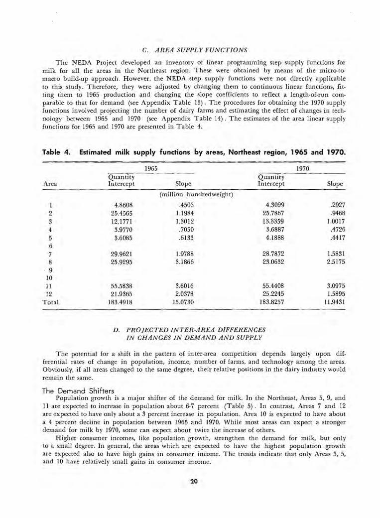
C. AREA SUPPLY FUNCTIONS

The NEDA Project developed an inventory of linear programming step supply functions for milk for all the areas in the Northeast region. These were obtained by means of the micro-to­macro build-up approach . However, the NEDA step supply functions were not directly applicable to this study. Therefore, they were adjusted by cha nging them to continuous linear functions, fit­ting them to 1965 production and changing the slope coefficients to reflect a length-of-run com­parable to that for demand (see Appendix Table 13). The procedures for obtaining the 1970 supply functions involved projecting the number of dairy farms and estimating the effect of changes in tech­nology between 1965 and 1970 (see Appendix Table 14) . The estimates of the area linear supply functions for 1965 and 1970 are presented in Table 4.

Table 4.

Area

1 2 3 4 5 6 7 8 9

10 11 12

Total

Estimated milk supply functions by areas, Northeast region,

1965 Quantity Quantity Intercept Slope Intercept

(million hundredweight)

4.8608 .4503 4.3099 25.4565 1.1984 25.7867 12.1771 1.3012 13.3359 3.9770 .7050 3.6887 3.6085 .6133 4.1888

29.9621 1.9788 28.7872 25.9295 3.1866 23.0632

55.5838 3.6016 55.4408 21 .9365 2.0378 25.2245

183.4918 15.0730 183.8257

D. PROJECTED INTER-AREA DIFFERENCES IN CHANGES IN DEMAND AND SUPPLY

1965 and 1970.

1970

Slope

.2927

.9468 1.0017

.4726

.4417

1.5831 2.5175

3.0975 1.5895

11.9431

The potential for a shift in the pattern of inter·area competition depends largely upon dif­ferential rates of change in population, income, number of farms, and technology among the areas. Obviously, if all areas changed to the same degree, their relative positions in the dairy industry would remain the same.

The Demand Shifters Population growth is a major shifter of the demand for milk. In the Northeast, Areas 5, 9, and

11 are expected to increase in population about 6·7 percent (Table 5). In contrast, Areas 7 and 12 are expected to have only about a 3 percent increase in population. Area 10 is expected to have about a 4 percent decline in population between 1965 and 1970. While most areas can expect a stronger demand for milk by 1970, some can expect about twice the increase of others.

Higher consumer incomes, like population growth, strengthen the demand for milk, but only to a small degree. In general, the areas which are expected to have the highest population growth are expected also to have high gains in consumer income. The trends indicate that only Areas 3, 5, and 10 have relatively small gains in consumer income.

20

Table 5. Projected changes affecting shifts in milk demand and supply between 1965 and 1970, by areas.

Projected change from 1965 to 1970a

Area Demand shifters Supply shifters

Resource Technological Population Consumer income base change change

growth change (Number of farms) (Output/farm change)

(percent) 1 5.9 11 -35 24 2 6.0 12 -21 23 3 5.5 5 -23 28 4 4.8 15 -33 19 5 7.8 8 ~28 31 6 4.4 13 7 3.6 13 ~20 16 8 6.0 13 -21 8 9 6.4 14

10 -3.9 7 II 7.2 14 -14 12 12 2.9 10 -22 33

a Percents calculated from data in Appendix Tables 3, 4, 11, and 12.

The Supply Shifters

In the Northeast, rapid declines in the number of dairy farms are expected to continue be­tween 1965 and 1970. A study by Kottke [13] has shown that the exit of farms in the proximity of expanding urban-industrial complexes withdraws resources from agriculture and, thereby, depresses supply, i.e., shifts the supply function backward. The highest rates of dairy farm exit are expected in Areas I, 4, and 5 where the projected rates are about 30 percent in five years. A relatively low exit rate of 14 percent is expected in Area II.

An offsetting factor to the decline in farms is technological change, which predominantly has an output-increasing effect. In this study, a proxy measure of technological changes, namely, change in output per farm, is used,15 The trends indicated that relatively high increases in output per farm can be expected in Areas 3, 5, and 12 where the increase is about 30 percent. In contrast, relatively low increases of 8-16 percent can be expected for Areas 7, 8, and II.

Over-all, the view of the changing Northeastern pattern of dairy trade seems to indicate that the intensive demand markets are spreading and the producing areas are contracting, thereby causing possible disruptions in the normal milk supply channels. Consequently, the area demand-supply balances are likely to be changed. In some of the Northeast areas, tighter milk supplies may tip the baJance toward more area deficits.

A Non-Equilibrium Projection of Milk Production and Consumption To obtain a cursory preview of the possible changes in area surpluses and deficits of milk pro­

duction, a non-equilibrium projection was made. Briefly, the procedure was to merely project each area's total production and consumption on the basis of the population, income, number of farms, and output per farm data used for shifting the demand and supply functions. In contrast to the spatial equilibrium analysis, the non-equilibrium projection omits price effects and inter-area flows of trade, i.e., price-quantity functions are not incorporated into the projection. The results of the non­equilibrium projection are shown in Table 6.

10 Calculated from NEDA advanced technology supply function data. See Appendix Tables 10 and II.

21

The most interesting possibilities indicated by the projected trends are as follows:

1. A combination of a moderate increase in consumption with a large decrease in production would cause Area 8 to change from relatively high surplus to low surplus and Areas 1 and 4 to increase their deficits.

2. A very small increase in consumption coupled with a 4 percent increase in production would cause Area 12 to maintain its small surplus.

3. High increases in consumption with small decreases in production would cause Area 5 to have a slightly larger deficit and Area II to have a substantiall y larger deficit in 1970.

4. Small to moderate increases in consumption coupled with small decreases in production would cause Areas 2 and 3 to remain nearly at their same surplus position as in 1965, while Area 7 would reduce its surplus moderately.

Table 6. Non-equilibrium projection of milk consumption and production from 1965 to 1970, by areas.

Projected percent changeo. Milk Milk

Area consumption production

1 5 -19 2 4 -3 3 4 -2 4 4 -20 5 6 5 6 10 7 3 8 8 4 -15 9 5

10 -13 II 6 -4 12 4

a Percents calculated from data in Appendix Tables 8, 13, and 14.

Surplus or deficit milk production

Projected 1965 1970

(million

3.41 26.53

9.69 -35.46 -ILl I

26.57 ILl8

-16.00 1.03

hundredweight)

- 5.36 25.56 9.00

-38.80 -12.64

23.31 4.17

-24.07 1.81

While the foregoing projection offers some clues to the possible outcome of inter-area changes, it provides only partial information. For a more inclusive analysis we need to turn to the spatial equilibrium model of this study. At this point, we would hypothesize that the incorporation of price effects as embodied in demand and supply functions will cause the equilibrium results to differ from the foregoing results of the non-equilibrium projection. One difference hypothesized is that with tight su pplies and expanding demands in the dairy industry, the model will generate higher equilib­rium milk prices which will simultaneously generate a greater quantity of milk. Thus, the projected changes in surplus and deficits may be expected to be tempered somewhat in the spatial equilibrium solution.

E. MILK SUPPLY FROM THE OUTSIDE REGION

Historically, a large proportion of manufacturing milk consumed in the Northeast has been im­ported from the Lake States and other regions outside of the Northeast region. In order to estimate the amount of imported manufacturing milk, the following procedures were used:

22

First, the total production of manufacturing milk in the Northeast was estimated. Then, this was subtracted from the total consumption of manufacturing milk, :lnd the difference was taken to be the import from the outside region. The following equations were used in making the estimate:

Tpm TP - (C + F) 1m = TCrn - Tpm

where:

Tpm = total production of manufacturing milk in the Northeast in 1965, TP total production of all milk in the Northeast in 1965, C = milk used to feed calves in 1965, F :=: milk used for human consumption in 1965, TCm :=: total consumption of manufacturing milk in the Northeast in 1965, 1m = import of manufacturing milk in the Northeast in 1965.

(45) (46)

The total 1965 production of manufacturing milk in the Northeast was estimated to be 86.2 mil­lion hundredweight. The amount of imported manufacturing milk was estimated to be 133.6 mil­lion hundredweight.

While most of the imported milk was manufacturing milk, some fluid milk also came from the outside region. In 1965, approximately 4.5 million hundredweight of fluid milk was imported from Virginia and West Virginia to the Northeast region,16 By adding the imported fluid milk and man­ufacturing milk together, total milk obtained from the outside region was estimated to be 138.1 mil­lion hundredweight. However, by subtracting the Northeast total milk production of 254.45 million hundredweight from the Northeast total milk consumption of 387.15 million hundredweight, one obtains a deficit of 132.7 million hundredweight. The reason for the discrepancy between the two estimates is not apparent. In the interest of using an estimate that balances the supply of milk with total consumption, the latter estimate of 132.7 million hundredweight was used.

The average milk price for the outside region was $3.10 per hundredweight. With two coordinates given, i.e., 132.7 million hundredweight and $3.10, the next step was to compute a supply equation through the coordinate point. The price elasticity of supply was assumed to be .28 which is the same as that for the Northeast aggregate milk supply. The resulting supply function for the outside re­gion is:

S = 95.5543 + 11.9857 V (47)

It should be noted that function (47) above is not a total milk supply function for the outside region, but rather, it is a net "flow to the Northeast region" supply function. It could be thought of as a net supply for shipment to the Northeast after the outside region's own demands have been met. For the purposes of this study, it is assumed that the outside region's £low of milk to the North­east region will remain relatively constant between 1965 and 1970; therefore, the same outside region supply function is used for both time points.

The elasticity used for the outside supply function was chosen largely arbitrarily. Since the func­tion is a net "£low to the Northeast" supply, the usual producer level elasticity is not entirely appli­cable. If it were, then the outside region's supply elasticity would be considered greater than that of the Northeast region. However, as an assumed "residual" milk supply, the outside region's quan­tity available for the Northeast may be considered relatively inelastic. As a consequence, the outside region supply elasticity was assumed the same as that for the Northeast.

IG Calculated from "Source of Milk for Federal Order Markets, by State and County," V.S.D.A. Consumer and Market­ing Service, Dairy Division, C&MS-50, September 1966. p. S.

23

F. TRANSPORTATION COSTS

The distances between most of the shipping points were directly obtained from highway maps. The transportation rates estimated in this study were based on an average hauling rate, that is, 37 cents per 100 pounds per 200 miles.

Given the mileage between any pair of shipping points and the transportation cost per unit, the total transportation cost between any two areas was estimated by the following equation: .

.$.37 tij := -- Mlj

(48) 200

where:

t!j total transportation cost between area i and area j Mij = mileage between area i and area j.

The inter-area mileages are shown in Appendix Table 9 and the results of applying equation (48) are shown in the transportation cost matrix of Table 7.

Table 7. Estimated transportation costs for milk, expressed in dollars per hundred pounds.

Area Area Outside and region city 2 3 4 5 6 7 8 9 10 11 12 Chicago

(1) Portland 0 .38 .34 .19 .38 .47 .44 .98 .59 1.12 .78 1.29 2.03

(2) Burlington 0 .12 .40 .42 .10 .27 .68 .56 1.17 .74 1.35 1.76

(3) Rutland 0 .29 .29 .19 .19 .65 .43 .83 .70 1.04 1.65

(4) Boston 0 .18 .47 .31 .84 .39 .93 .57 1.10 1.83

(5) Hartford 0 .47 .19 .71 .21 .89 .39 .93 1.71

(6) Saranac Lake 0 .29 .60 .56 1.07 .74 1.16 1.70

(7) Albany 0 .52 .28 .59 .45 .84 1.50

(8) Buffalo 0 .68 .19 .68 .41 .98

(9) N. Y. City 0 .52 .17 .70 1.46

(10) St. Mary 0 .37 .19 .96

(11) Philadelphia 0 .54 1.32

(12) Pittsburgh 0 .87 Outside-region

Chicago 0

24

v. QUADRATIC PROGRAMMING SOLUTIONS

A. THE 1965 OPTIMUM SPATIAL EQUILIBRIUM SOLUTION

Information obtained from the quadratic programming solution is presented in Table 8. The optimum solution indicates what the prices, production, consumption, and flows of trade should have been in 1965, subject to the conditions and assumptions discussed in the preceding section. In evaluating the solution, one should bear in mind that perfectly competitive behavior was assumed and that the flow of milk from the outside region was assumed to be relatively inflexible. Moreover, a zero price differential between fluid and manufacturing milk was assumed. Therefore, the solu­tion can be considered conditionally normative.

Tab~e 8. Spatial equilibrium production and consumption, by areas, 1965.

Destination

Origin

(1) Portland

(2) Burlington

(3) Rutland

(4) Boston

(5) Hartford

(6) Saranac Lake

(7) Albany

(8) Buffalo

(9) N. Y. City

(10) St. Mary

(11)

2 3

6.72

3.29 4.15

8.26

Area 4 5 6 7 8 9 10 II 12 Total

prod. (million hundredweight)

6.72

21.65 .98 30.07

9.08 17.34

6.98 6.98

6.15 6.15

11.43 11.84 37.79 3.23 11.29

28.17 9.09 37.26

70.32 70.32 Philadelphia ----;(7::12",..)-=------------------------------;2lii9~.3"5 29.35

Pittsburgh

Outside Region

Total consumption

lll.07 2.19 14.69 .79 128.74

10.01 4.15 8.26 40.94 17.44 .98 11.43 28.17 132.00 2.19 85.Ql 30.14 370.72

25

The optimum solution could be expected to differ from the "real" measurements of the dairy industry in 1965. On the other hand, the results could be expected to be reasonably close to the 1965 actual situation because the data employed in the model were developed, in part, from observed data. As long as the model is reasonably representative of the benchmark situation, then it may serve as an estimator of the consequences of economic changes between 1965 and 1970. In the following presentation of the results, the representativeness of the model is evaluated by comparisons between the optimum solution and the benchmark data.l7

Prices The optimum prices within the Northeast region range from $3.55 to $4.26 per hundredweight

of milk (Table 9). The optimum price of milk shipped in from the outside is .$2.77 per hundred­weight. The highest price is in Area 4 and the lowest price is in Area 8. Basically, the inter-area price differentials represent the costs of transportation involved in inter-area flows of trade. Since baniers to inter-area trade are assumed non-existent, competitive price advantages are non-existent in the optimum solution. The optimum price is a single product price at the farm level. Its bench­mark counterpart is an approximate blend price (weighted average of fluid and manufacturing milk prices) . In general, the benchmark prices are about $1.00 higher than the optimum 1965 prices. While the solution prices are not close to the benchmark prices, the rankings of areas from high to low prices are quite close. Only Areas 5, 6, and 12 are noticeably uncorrelated in the two rankings. How­ever, the crudeness of the estimating procedure used for obtaining the benchmark prices may con­tribute to the variation. Except for this limitation, the optimum solution may suggest which areas have overpriced or underpriced milk relative to what the price would have been if perfectly com­petitive conditions had prevailed in 1965.

Table 9. Ranking of areas in terms of milk prices, 1965. Benchmark Optimum

Rank Area price - 19659, Area milk price

1 5 ($ per cwt.) ($ per cwt.)

5.61 4 4.26 2 4 5.59 1 4.24 3 1 5.35 9 4.23 4 9 5.08 5 4.15 5 II 5.00 11 4.09 6 3 4.90 3 3.97 7 2 4.60 6 3.96 8 12 4.55 7 3.95 9 7 4.50 2 3.86

10 10 4.50 10 3.73 11 6 4.45 12 3.64 12 8 4.40 8 3.55 13 Outside 3.10 Outside 2.77

region region

a Approximated from 1965 milk prices on a state basis. Source: Milk Production, Disposition, and Income 1961-65, V.S.D.A. Statistical R eporting Servic;e,

Crop Reporting Board, Washington, D. C.

Consumption The optimum consumption of milk is 370.7 million hundredweight, compared with 387.2 mil-

[7 The benchmark production and consumption data for 1965 are essentially the same data used to obtain the price­quantity coordinate points in constructing the demand ;md supply functions. They are area estimates ()btained largely from state and national data which were observed for 1965. The 1965 benchmark production data are estimates pro· jected largely from 1961 observations. The benchmark prices are approximations of the blend prices for each area.

26

lion hundredweight calculated for the 1965 benchmark (Table 10). This amounts to a 4 percent underestimation. One important difference between the optimum and the benchmark data is that consumption of manufacturing milk is less and fluid milk is greater than the benchmark con­sumption. This difference stems from the assumption of a zero price differential.

In actuality, a price differential exists. Thus, the model's zero price differential results in a price which is lower than the fluid price and higher than the observed manufacturing price. Observed prices were used in positioning the demand functions. The obvious effect of a single in-between price is that less manufacturing and more fluid milk is demanded. Furthermore, since the demand for fluid milk is relatively inelastic and the demand for manufacturing milk is relatively elastic, the quantity of manufacturing milk decreases more than the quantity of fluid milk increases; thereby, a net decrease in total milk demanded results.

Production The optimum solution suggests that 242 million hundredweight of milk should have been pro­

duced in the Northeast in 1965. In comparison, the benchmark production was 254.4 million hun­dredweight. The explanation of this discrepancy is tied in with the explanations covering the dis­crepancy involving consumption. Possibly there is a further explanation, though, on the production side. Apparently, the procedure used for constructing the supply functions contributes to the under­estimation of optimum production.

Table 10. Comparison of the 1965 optimum and benchmark production and consump­tion data.

Consumption of Consumption of Area fluid milk manufacturing milk Production

Benchmarka. Optimum Benchmarka Optimum Benchmark Optimum

(million hundredweight) I 4.78 4.93 5.88 5.08 7.25 6.72 2 1.67 1.70 2.69 2.45 30.89 30.07 3 3.35 3.43 5.40 4.83 18.44 17.34 4 19.05 19.83 24.35 21.11 7.94 6.98 5 8.41 8.78 9.74 8.66 7.04 6.15 6 .45 .46 .59 .52 7 5.43 5.49 6.53 5.94 38.53 37.79 8 11.82 12.08 16.73 16.09 39.73 37.26 9 58.38 58.07 80.08 73.93

IO 1.00 1.02 1.24 1.17 II 39.42 40.33 49.70 44.68 73.12 70.32 12 13.57 14.01 16.91 16.13 31.51 29.35

ORb 132.70 128.74 Total 167.33 170.13 219.82 200.60 387.l5 370.73

a Obtained from Appendix Table 8. b From outside of the Northeast region.

The coordinate price-quantity point used was the 1965 blend price and the estimated 1965 pro­duction. To this coordinate point the slope of the supply function (i.e., marginal cost function) was fitted. If, in fact, an element of imperfect competition exists in the dairy industry, then the blend price-quantity coordinate lies above the marginal cost at that quantity. Accordingly, the slope of the supply function should probably have been fitted to a point to the right of and below the blend price-quantity point. Most likely, the optimum production would then have exceeded the benchmark production and, correspondingly, would have fulfilled the implication of a perfectly com­petitive versus an imperfectly competitive solution, i.e., greater output for the perfectly competitive solution.

27

Surplus and Deficit Production Areas The optimum solution surplus and deficit areas are the same as the benchmark ones for 1965,

except Area 12 which is a deficit area in the optimum solution and was a surplus area in 1965 accord­ing to the benchmark data. The other deficit Areas are 1, 4, 5, 6, 9, 10, and 11.

Within the Northeast region, inter-area shipments of milk involve eight flows of trade accord­ing to the optimum solution (Figure 3). Six of the flows originate in Areas 2 and 7. The largest inter-area flow is from Area 2 to Area 4. The spatial equilibrium model directs most of outside re­gional milk to New York City (in Area 9) and smaller amounts to Areas 10, 11, and 12.

Over-all Representativeness of the Benchmark Model While the optimum solution is not in perfect correspondence with the benchmark data, it is suf­

ficiently close so that the model may be used for a comparative statics analysis. However, evalua tion of the results of the analysis should take into account all of the model's assumptions.

B. THE PROJECTED 1970 SPATIAL EQUILIBRIUM SOLUTION The projections of changes in population, income, number of farms, and technology are ex­

pected to alter the competitive positions of the Northeast dairy areas by 1970. A non-equilibrium pro­jection was presented in Section IV, D. Now we turn to the spatial equilibrium projection which takes into account price effects and inter-area flows of trade. The spatial equilibrium model for 1970 incorporates the projected (shifted) demand and supply functions.

Prices As hypothesized in the non-equilibrium projection in Section IV, D, the tighter mjlk supplies

and expanding demands generate higher equilibrium prices for 1970 (Table 11). In general, the prices are $.52 per hundredweight higher for all areas, except Area 12 ($.43 higher). The range is $4.07-$4.78. Since the milk price increases by the same amount in all areas except Area 12, the rank­ing of areas in terms of price remains essentially the same. The only change in ranking is that Area 12 drops to the lowest price area and thereby changes places with Area 8. This demonstrates an important property of a perfectly competitive spatial equilibrium model. The property is that inter-area price differentials represent only the costs of transportation for inter-area flows of trade. The only way that inter-area price differentials can change, one relative to another, is by a change in the direction of flow of trade. That is what occurs to Area 12 in the optimum solutions as it changes from a deficit area for 1965 to a surplus area for 1970 (Tables 12 and 13) .

Table 11. Ranking of areas in terms of optimum milk prices, 1970.

Optimum milk Rank Area price for 1970

($ per cwt.) 1 4 4.78 2 1 4.76 3 9 4.75 4 5 4.67 5 11 4.61 6 3 4.49 7 6 4.48 8 7 4.47 9 2 4.38

10 10 4.25 11 8 4.08 12 12 4.07 13 Outside region 3.28

28

Figure 3. - Optimum pattern of milk

shipment for 1965 under assumption

of perfect competition conditions.

Outside Region

(Chicago)

29

Table 12. Change in milk consumption and production between 1965 and 1970 as de­rived from the spatial equilibrium solutions, by areas.

Percent change 1965-1970 Surplus or deficit Area Milk Milk milk production

consumption production 1965 1970

(million hundredweight) I 0 -15 3.29 - 4.31 2 -2 0 25 .92 25.85 3 1 3 9.08 9.64 4 - 1 -15 33.96 34.57 5 1 2 11.29 11.43 6 7 .98 1.05 7 -2 - 5 26.36 24.64 8 0 -11 9.09 5.27 9 1 -132.00 -133.32

10 -18 2.19 1.80 11 1 - 1 14.69 16.21 12 - 3 8 .79 2.33

Consumption and Production Most of the areas show only a slight change in consumption. Areas 5, 6, 9, and 11 show an in­

crease; Areas 1 and 8 remain unchanged. As shown in Table 12, percentage decreases of 1-3 percent and increases of 1 percent dominate. In contrast, the non-equilibrium projection (Table 6, Section IV, D) indicated potential increases of 4-6 percent in milk consumption for most areas.

The change in optimum production between 1965 and 1970 plays a major role in the over-all outcome. Five of the areas show a decrease in production. They are Areas I, 4, 7, 8, and II. Only three areas show an increase. However, the general tightness of supply for 1970 is not as severe in the spatial equilibrium solutions as in the non-equilibrium projection (compare Tables 6 and 12). This difference demonstrates one of the features of the spatial equilibrium model, i.e ., its ability to in­corporate the effect of prices to generate a change in production . As a consequence, the optimum solutions indicate less change in the surplus and deficit positions than that estimated by the non­equilibrium projection.

Surplus and Deficit Production Areas All of the areas, except Area 12, remain surplus if they were surplus and remain deficit if they

were deficit. However, they change in the magnitude of their surplus or deficit. Moreover, the direc­tion of change varies among the areas. The following changes between 1965 and 1970 are indicated by the spatial equilibrium analysis:

1. A combination of no change in consumption and a large decrease in production would cause Area 8 to decrease its surplus moderately. The same conditions would cause Area I to increase its deficit slightly. Area 4: with similar conditions would maintain its deficit.

2. A small decrease in consumption, coupled with a large increase in production would cause Area 12 to change from a slightly deficit area to a surplus area.

3. A very small increase in consumption, coupled with a very small change in production would cause Area 5 to maintain a nearly constant deficit and Area 11 to have a small in­crease in its deficit.

30

4. A combination of a small decrease in consumption and either no change or a small in­crease in production would cause Areas 2 and 3 to remain at nearly the same surplus posi­tion as in 1965. Area 7 with a small decrease in consumption but a moderate decrease in production would have a small decrease in its surplus position.

The foregoing list of changes can be compared with those listed in Section IV, D for the non­equilibrium projection. In general, the results are similar except that the changes in surplus or deficit are tempered in the spatial equilibrium analysis, compared to those in the non-equilibrium projection. An overview comparison of the two sets of results is presented in Table 14. The most obvious difference is that Area II shows only a small deficit increase in the spatial equilibrium analysis, whereas in the non.equilibrium projection, it showed a substantial increase in deficit.

Table 13. Spatial equilibrium production and consumption, by areas, 1970.

Area Destination 2 3 4 5 6 7 8 9 10 II 12 Total

Origin prod. (million hundredweight)

(1) Portland 5.70 5.70

(2) Burlington 4.31 4.08 20.49 1.05 29.93

(3) Rutland 8.19 9.64 17.83

(4) Boston 5.95 5.95

(5) Hartford 6.25 6.25

(6) Saranac Lake

(7) Albany 4.44 11.43 11.23 8.77 35.87

(8) Buffalo 28.05 5.27 33.32

(9) N. Y. City

(10) St. Mary

(11 ) Philadelphia 69.72 69.72

(j 2) Pittsburgh 2.33 29.36 31.69

Outside Region 119.28 1.80 13.88 134.97

Total consumption 10.01 4.08 8.19 40.52 17.68 1.05 11.23 28.05 133.32 1.80 85.93 29.36 371.23

31

Table 14. Comparison of changes in area milk surplus or deficit production 1965-1970, derived from the non-equilibrium projection and the spatial equilib­rium analysis.

Changes in milk surplus or deficit

I. Decrease in surplus Substantial Moderate Small

2. Increase in deficit Su bstan tial Moderate Small

3. Essentially no change 4. From deficit to surplus

Non-equilibrium projection

8 7

11 I

4,5 2,3,12

Areas involved . Spatial equilibrium

analysis

8 7

I,ll 2,3,4,5

12

Within the Northeast region, one more flow of trade is added for 1970 to the eight that existed in the 1965 benchmark solution (Figure 4). The new flow of trade originates in Area 12 and goes to Area II. Another significant change is that the quantity of milk in the £low of trade from Area 8 to Area 9 is nearly cut in half. Otherwise, the inter-area shipments of milk remain practically un­changed between 1965 and 1970.

VI. SUMMARY AND CONCLUSIONS In the Northeast region, population growth is expanding the market for dairy products, while

the number of dairy farms is declining rapidly and, thereby, restraining growth of the milk supply. Changes in population, consumer income, number of farms, and technology are occurring unevenly among the areas in the region. In general, the intensive-demand markets are spreading, while the producing areas are contracting. These differential rates of change are expected to continue in the near future and cause possible disruptions in the normal milk supply channels. It is hypothesized that some of the areas in the Northeast can expect tighter milk supplies and, consequently, milk pro­duction-consumption balances will tip toward deficit production in more areas.

In order to analyze the foregoing problem, a comparative statics approach involving two spa­tial equilibrium points .vas used. The year 1965 was designated the first point in time. A spatial equilibrium solution of optimum milk prices, flows of trade, production and consumption were obtained by utilizing current data for that date and by employing a quadratic programming for­mulation. Milk demand and supply functions were estimated for each of the 12 areas designated for the study. A net import supply function for milk shipped into the Northeast from outside regions was also estimated. The optimum solution for 1965 was compared with benchmark data for 1965 to ascertain the model's representativeness of the actual dairy situation. Except for qualifications imposed by the assumption of perfect competition, the model was judged to be reasonably close as an approximation of the Northeast dairy situation.

The future date of 1970 was designated the second point in time of the comparative statics anal ysis. In order to estimate the potential milk demand and supply functions for 1970, it was necessary to project population growth, consumer income, number of farms, and output per farm for each of the areas. The projection of these factors was the means used to incorporate the expected differential shifts in supply and demand among the areas. A comparison of the projected 1970 solution with the 1965 solution indicated the following:

32

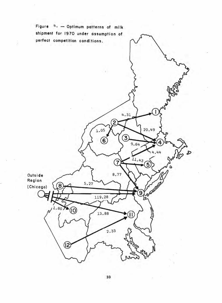
Figure 4. - Optimum patterns of milk

shipment for 1970 under assumption of

perfect competition conditions.

Outside Region

(Chi cogo)

QJ

33

1. The 1970 spatial equilibrium prices were about $.50 per hundredweight (about 12 per­cent) higher than the 1965 solution prices.

2. The tightening of the milk supply played a major role in the over-all outcome. Five of the 9 production areas showed a decrease in production. As a consequence, the projected equil­ibrium milk consumption was generally less area by area than that projected on the basis of population growth and per capita consumption alone.

3. Only one of the areas showed a change in its production-consumption balance. Area 12 (Pittsburgh, Penn. vicinity) changed from deficit to surplus production. This stemmed from a 3 percent decrease in demand, coupled with an 8 percent increase in supply in that area.

4. Area 8's (Buffalo, N. Y. vicinity) milk surplus was reduced noticeably. The other areas changed only slightly or remained unchanged in their production-consumption balance.

5. The total quantity of milk demanded in the Northeast increased only .5 million hundred­weight (.1 percent) from the 1965 solution to the 1970 solution. Obviously, with an ex­pected 5-6 percent growth in population and essentially no change in total milk consump· tion by 1970, per capita milk consumption would decrease. Currently, it seems plausible that such a consequence may actually occur because the trend in per capita consumption of milk and milk products is downward.

The results of this study are conditioned by the assumption that perfect competition prevails in the dairy industry. In actuality, a price differential exists between fluid and manufacturing milk. Federal Milk Marketing Orders regulate the pricing of fluid milk. Accordingly, the assumption of perfect competition oversimplifies the actual dJ.iry market behavior.

A refinement of this study's spatial equilibrium model to incorporate some of the pricing in­tricacies would be appropriate and is suggested for further research. The inclusion of recursive concepts would improve the model. The demands for fluid and manufacturing milk should probably be separated with respect to tentative ·equilibrating points in time and space. In an actual market, the price and quantity of manufacturing milk is determined by a residual process, i.e., the price and quantity of fluid milk is determined separately and administered so as to stabilize the fluid milk market. The residual milk, after the fluid milk demand is met, is then diverted to manufacturing uses.

The recursive concept of the proposed model would have the subsequent outcome of one prod­uct (manufacturing milk) dependent upon the previous outcome of the other product (fluid milk). Such a procedure would capture the inter-product price differential effect which was omitted in this present model.

The Takayama-Judge quadratic programming formulation and Moffett's computer program proved to be efficient and reliable tools for spatial equilibrium analysis. The operational competence of these tools engenders promise of productive effort in further investigations of interregional com­petition problems. Heretofore, researchers had to be content with piecemeal and step-wise methods of analyzing spatially separated-but inter-depenclent-markets. Now, with quadratic programming, it is possible to simultaneously solve complex equilibrium problems involving sets of continuous linear functions. Moreover, when quadratic programming is used in conjunction with a comparative statics approach, it is possible to incorporate the integrated effects of both (1) producers' and consumers' responsiveness to price, and (2) the shifts in demand and supply caused by population growth, changes in consumer income, changes in number of firms, and changes in technology.

34

APPENDICES

Appendix Table 1. Demarcation of the Northeast areas by redefinition of the NEDA areas

NEDA Areas of this study

areas al Area Identitx Eoint

1, 2 1 Portland, Me. 4, 7, 10 2 Burlington, Vt. 5, 8, 9 3 Rutland, Vt. 3 4 Boston, Mass. 6 5 Hartford, Conn. F 6 Saranac Lake, N. Y. 11, 13 7 Albany, N. Y. 12, 14 8 Buffalo, N. Y. I 9 New York, N. Y. J 10 St. Mary's, Penn. 17, 18, 19, 20 11 Philadelphia, Penn. 15, 16 12 Pittsburgh, Penn.

al See the NEDA planning data bulletin [17].

35

Appendix Table 2. Projected population estimates for the Northeast region, by areas and residence group, 1965 and 1970

Area

1 2 3 4 5 6 7 8 9

10 11 12

Total

Urban

817,501 218,518 673,521

4,903,250 2,052,761

54,477 999,341

2,644,546 17,414,717

144,812 9,444,963 2,828,274

42,206,681

Population

1965

Rural ' Rural ' non-farm ' farm Urban

657,489 47,546 864,530 258,206 54,184 228,101 356,202 32,338 706,570

1,059,811 35,991 5,136,435 575,584 25,409 2,214,520

73,074 5,731 65,846 649,603 75,960 1,045,708 925,073 109,456 2,789,127 827,772 11,948 18,603,392 167,338 9,654 136,010

2,680,765 295,621 10,199,790 1,357,169 113,189 2,898,628 9,588,086 817,027 44,888,657

1970

Rural ' Rural ' non-farm ' farm

720,546 26,524 293,805 40,734 390,764 23,621

1,118,388 31,997 625,722 20,825

80,812 2,993 694,544 45,901

1,049,289 60,681 823,549 0 166,922 6,182

2,867,345 245,707 1,463,369 60,953

10,295,055 566,118

Source: P. S. Dhillon, "Estimation of Demand Functions," mimeographed report presented to NEDA Committee, Pennsylvania State Univer­sity, 1965. Projected estimates were obtained from the U. S. Census, Population Estimates, Series P-25, No. 301, February 1965. Allocation of the projected estimates among the areas and residence groups was based on proportion of population in each area and residence group in the years 1940, 1950, and 1960. The NEDA areas used in Dhillon's estimates have been redefined for this study (Appendix Table 1).

36

Appendix Table 3. Projected population estimates for the Northeast region, by areas, 1965 and 1970

POEulation

Area Percent Projected change

1965 1970 1965-70

1 1,522,536 1,611,600 5.85 2 530,908 562,640 5.98 3 1,062,061 1,120,955 5.54 4 5,999,052 6,286,820 4.80 5 2,653,754 2,861,067 7.81 6 143,282 149,651 4.44 7 1,724,904 1,786,153 3.55 8 3,679,075 3,899,097 5.98 9 18,254,437 19,426,941 6.42

10 321,804 309,114 -3.94 11 12,421,349 13,312,842 7.17 12 4,298,632 4,422,950 2.89

Total 52,611,794 55,749,830 5.96

Source: P. S. Dhillon <See Appendix Table 2).

37

Append'l¥%Drr~ '4~ J 'py.6Je'C~J· ~e~'tiIjH~-\:~%·L6'f; pefr~" caplta ~ disposa¥"i~ t>'et!Sonal inc~~~l, '~oif-thi'ast, r~&l-on"O by'areas, 1965 and 1970

Ar~R-.').Yleq

:9~D6[b

~-2a(?1

1 C • C 2 Be. ~

j.J.~ < ;: 3 4 08. l-S .£ • ';' 6 j.! j" . 1J

7 CC . C 8 ae. (; 9 S+l . a

10

bSj :)9 t 0'1'1

196 50'\e f 1970

Percent change 1965-(!,92 1

Percent change multiplied 68'1.1

by income elasticity (.06)

.0068

.0070

.0031

.0087

.0050

.0077

.0080

.0080

.0081

.0044

.0084

.0058

1

c

B (.'

,',

~' l

l.s:to'f

source :"--P':-S:" -uniIIon~"'ffES;e;:rmat~o~ ~r De~?!laTuric?p?~ ~ :'-m:fmec?gr~?~;d ,~ report presented to'" Nt.ffAs COfufrll~"; Wnhso/lva~ S::tate Un'l:VeiQ..'-' sity, 1965. The method of estimation involved using county personal income data reported in Sales Management published by Bill Brothers. The 1965 and 1970 estimates were extra­polated on a trend line based on 1957 and 1963 data. The NEDA areas used in Dhillon's estimates have been redefined for this study (See appendix Table 1).

Appendix Table 5. Projected consumption of fluid milk, by areas and residence groups, Northeast region, 1970

q \

VbbsJ)qpt J.9PJ Co 2" ( COU q-UIJ6q)

"j '

1. a1a83 2 1.:tl'Q"Wfi? 8 1 .1l'J-'VlB S 1.~a'OJ'7.:o? 8 .rr~a 1 .10t)Y,b?9

1.04YaTS 1 • J{)"03J!3 It 1 Jb"g:.'iJ:03 e 1.10'0:3'3131'1

.J7'3.1J'H3 a 1.10"013.180

1. ()"!fli6"Jrt 1 JO'cJ.8J7. t It 1.0'5'@21 2 1 .JO'CfHJl,1 rr

. 8"was 1 JO'OBJJt rt

1.C0788 1 .J0'0IDIl T a 1.O'ffm]rt3 IJO'0IDJ3T

J8'JOJ.633 1.JO'cm:m r

1. O'::H.,J],f \t 1.100Rm 1.Jl'05Bt3 lJO'ClW

J5'ILf2H? 1 JUOJlJB

.9985

.9970 1-:- 0--

.19'gB 5

.9Wcm 1. 0' aaS 2

.J9'9:85

.9'917dll O 1. O' 8 iJ S?

.}9'9.'B5 • g"gJ7(Oi 0

1. O' aa8;?

:]9'9:8 5 .g9m

1. (j a a8!?

$9:85 .g9)ID

1. 0' 3.1 l32

". :57.a:~

, I ".!89B'H ( -.l:.4:lll

2.lQ.6'B9 If .,'l.813::V

3~ .iDJE..'5

16' .(5'8l4-8 3·.~DJiO

•• rd?J.:a9

07 .1245 ;;;r .cB::9:9;9

e O'IOf1iQU

":'2lJ26 ;; . :12.#ffB 8' .:mlaJJ.+

5.0689

1 :r.C7LO':R8

!1$.i8'3::-4ft.

20'.am~

eS.m15f6

T:S"~

1.0464 1.008 .9985 ( LU r3r.3~::;i,~( ·) ( WTJ" C oU' )

~t{)q~~ rav - ~llJ6 .:;:---~7~6?' "~.m~ . \ .~ 64~~ I

~':!L ___ £1\.008 P\ 1.0 G\ i 62'J~~6 ~LOJG':::'-: TiJFCOE;-r - . T CT GlJ.j:G .) "' D •• t t . , _ _ _

cou3IJwb.Q·ou "<1\ bI,O ~Gq: hq Ta.'JO

.. .i.c oQj: i n1t~_<1L-

". o

Appendix Table 5. (Continued)

Residence 1965 Projectin~ coefficients

Area PODu1ation ~/ Income £!

8 Urban 8.4784 1.0546 1.008 Rural non-farm 2.9686 1.1343 1.008 Rural farm .3765 .5544 1. 008

9 Urban 55.8316 1. 0683 1.0081 Rural non-farm 2.5073 .9943 1.0081 Rural farm .0411 0 1. 00819

10 Urban .4643 .9392 1.0044 Rural non-farm .5069 .9975 1. 0044 Rural farm .0332 .6404 1.0044

11 Urban 30.2806 1. 0799 1.0084 Rural non-farm 8.1200 1. 0696 1.0084 Rural farm 1. 0169 .8312 1.0084

12 Urban 9.0674 1. 0249 1.0058 Rural non-farm 4.1109 1. 0782 1.0058 Rural farm .3894 .5385 1. 0058

~ Based on population projections as presented in Appendix Table 3. £! Based on income projections as presented in Appendix Table 4.

Tastes ~

.9785

.997 1.0

.9985

.997 1.0

.9985

.9970 1.0

.9985

.9970 1.0

.9985

.997 1.0

Projected 1970 consumEtion ~/

Residence grouE Area

mil. cwt.

8.9993 3.3840 12.5937

.2104

60.0485 2.5057 62.5541 0

.4373

.5059 .9646

.0214

32.9252 8.7319 42.5094

.8524

9.3331 4.4447 13.9887

.2109

c/ Estimated per capita consumption change due to change in tastes as follows: urban = -0.15%, rural non­farm = -0.3%, rural farm = no change. Obtained as the residual effect after deducting for income and price elasticity effects on the change in per capita consumption between 1956 and 1965 (from 333.9 to 320.6 1bs. for urban population and from 315.5 to 302 for the rural non-farm population).

d/ Average per capita fluid milk consumption for 1970: 17829.790 ~ 55.749 = 319.8.

Appendix Table 6. Estimated demand functions for fluid milk by areas, Northeast region, 1965 and 1970 ~/

Area

1 2 3 4

5 6 7 8 9

10 11 12

Quantity Intercept

5.5435 1.8978 3.8354

22.2605 9.8255

.5098 6.1432

13.3387 66.1757 1.1424

45.1711 15.4893

1965

Slope (million

- .1448 - .0505 - .1010 - .5706 - .2524 - .0136 - .1641 - .3499 -1. 7362 - .0306 -1.1814 - .4088

1970

Quantity Intercept Slope

hundredweight)

5.8813 - .1533 2.0122 - .0535 4.0469 - .1066

23.4628 - .5979 10.6195 - .2721

.5336 - .0142 6.3833 - .1698

14.1995 - .3708 70.8505 -1.8477 1. 0972 - .0294

48.6759 -1.2662 15.9658 - .4206

a/ The method of estimation was as follows: (1) the quantity of milk consumed as presented in Appendix Table 5 was used as a quantity point for each area function, (2) Brandow's [4, p. 112-113J slope coeffic­ient was applied to obtain a slope coefficient for each area, and (3) the area slope coefficient and the area quantity point were set in equation form to solve for the intercept value.

41

Appendix Table 7. Estimated demand functions for manufacturing milk by areas, Northeast region, 1965 and 1970

Area

1 2 3 4 5 6 7 8 9

10 11 12

Total

Quantity Intercept

8.499 3 , 829 7.586

34.636 13.950

.825 9.256

23.603 114.911

1. 799 71. 369 24.423

314.686

1965

Slope (million

.8061

.3570

.6938 - 3.1759 - 1. 2753

.0755

.8402 - 2.1161 - 9.6878

.1695

- 6.5261

- 2.2770 -28.180

1970

Quantity Intercept Slope

hundredweight)

8.924 .8532 3.954 .3771 7.938 .7377

35.819 - 3.3283 14.744 - 1.3745

.933 .0788 9.552 .8827

24.427 - 2.2238 120.742 -10.4217

1.523 .1628 75.249 - 6.9754 24.619 - 2.3398

328.424 -29.7561

Source: P. S. Dhillon, "Estimation of Demand Functions," mimeographed report presented to NEDA Committee, Pennsylvania State Univer­sity, 1965. All functions except those for Areas 6 and 10 were obtained directly from Dhillon's report. The functions for Areas 6 and 10 were obtained by first estimating a 1965 quantity point of manufacturing milk consumed in an area by mUltiplying per capita consumption rates by population for each residence group in an area. Second, the Brandow [4, p. 112J slope coefficient was applied to the area to obtain the area slope coefficient. Third, the area slope coefficient and the area quantity point were set in equation form to solve for the intercept value.

42

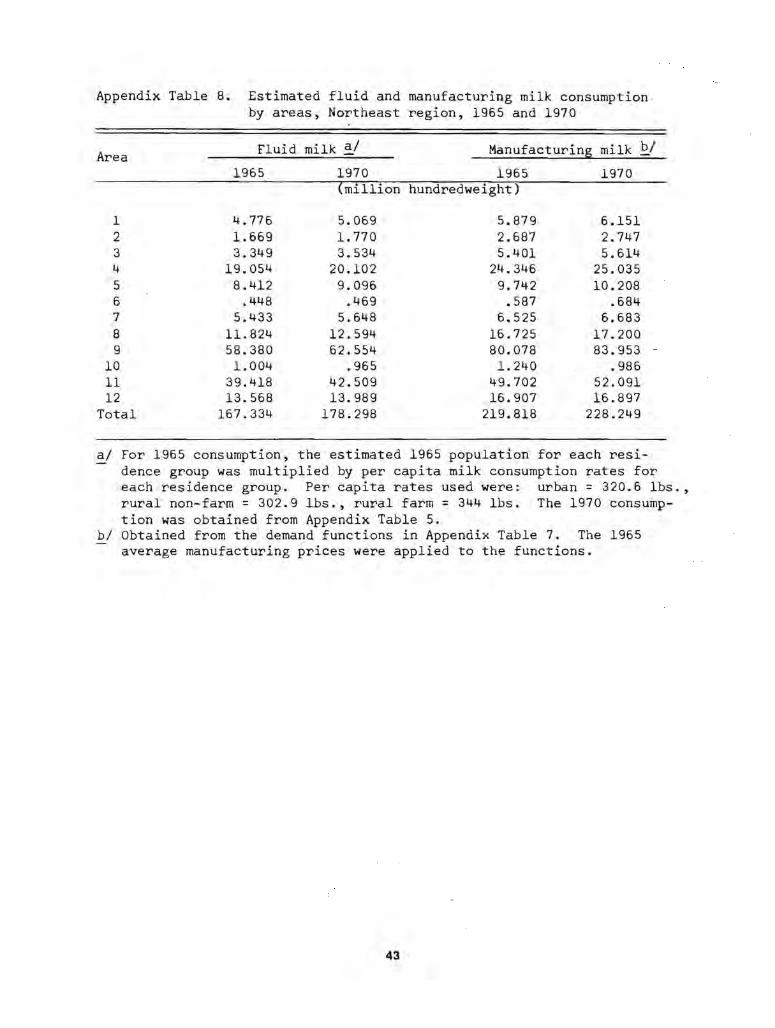
Appendix Table 8. Estimated fluid and manufacturing milk consumption by areas, Northeast region, 1965 and 1970

Area Fluid milk al Manufacturin~ milk bl

1965 1970 1965 1970 (million hundredweight)

1 4.776 5.069 5.879 6.151 2 1.669 1. 770 2.687 2.747 3 3.349 3.534 5.401 5.614 4 19.054 20.102 24.346 25.035 5 8.412 9.096 9.742 10.208 6 .448 .469 .587 .684 7 5.433 5.648 6.525 6.683 8 11. 824 12.594 16.725 17.200 9 58.380 62.554 80.078 83.953

10 1.004 .965 1. 240 .986 11 39.418 42.509 49.702 52.091 12 13.568 13.989 16.907 16.897

Total 167.334 178.298 219.818 228.249

al For 1965 consumption, the estimated 1965 population for each resi­dence group was multiplied by per capita milk consumption rates for each residence group. Per capita rates used were: urban = 320.6 Ibs., rural non-farm = 302.9 Ibs., rural farm = 344 Ibs. The 1970 consump­tion was obtained from Appendix Table 5.

bl Obtained from the demand functions in Appendix Table 7. The 1965 average manufacturing prices were applied to the functions.

43

Appendix Table 9. Mileage between area identity points, Northeast region and Chicago, Illinois

Milea~e to area identit~ Eoint

III .r-!

I:: 00 .c .c 0 . 0. bO

'U +-' 'U ~ ~ .-I ~

I:: bO 'U ~ U 0 ~ III ;:1

I1l I:: I:: I:: 0 III » .-I 0 I1l 'U .Q

.-I 'r-! III 0 lH I:: I:: I1l >< :E III rJl

+-' .-I .-I +-' +-' III III I1l lH .-I +-' ~ ~ +-' 00 ~ ~ ~ .Q lH ~ . • .-1 +-'

Area 0 ;:1 ;:1 0 ~ ~j .-I ;:1 Q) +-' .c .r-!

Il.. ~ ~ ~ < ~ z U) Il.. Il.. Area identity

Eoint 1 2 3 4 5 6 7 8 9 10 11 12

1 Portland, Me. 205 185 105 205 255 240 528 320 605 421 695 2 Burlington, Vt. 65 215 225 55 145 370 300 630 400 730 3 Rutland, Vt. 155 155 100 100 350 235 450 380 560 4 Boston, Mass. 100 255 165 455 210 500 308 595

"" 5 Hartford, Conn. 255 105 385 115 480 209 503 "" 6 Saranac Lake, N. Y. 156 326 305 580 400 626

7 Albany, N. Y. 280 150 320 243 454 8 Buffalo, N. Y. 365 105 365 222 9 New York, N. Y. 280 94 376

10 St. Mary's, Penn. 200 100 11 Philadelphia, Penn. 294 12 Chicago, Ill. 1095 950 890 990 925 920 810 530 790 520 720 470

Source: Estimated by use of 1966 U. S. Highway MaE, Humble Oil and Refining Company, produced by General Drafting Company, Inc., New Jersey.

Appendix Table 10. Estimated milk output per farm based on the NEDA

, ,NEDA

Area'

1 2 3 4 5 6 7 8 9

10 11 12

'61 base - '68 technology supply function, by areas, at the average 1961-65 price, Northeast region

, Aggregate 'Output per '61 base-'68 technology, Average , 1968 output 'farm based supply function~ price , of milk with , on 1961

Quantity , of milkbl

, 1961 number 'number of intercept Slope 1961-65=-: of farms farms

(million cwt. ) ($ per cwt.) (million cwt.)(thous. cwt. )

5.015 1.6735 5.30 13.8846 3.6347 30.180 3.4785 4.53 45.9376 3.9296 12.242 4.6595 4.81 34.6542 4.3421

.065 2.3925 5.62 13.5109 4.5036 1.043 1. 9515 5.60 11. 9714 5.4194

33.684 6.4200 4.33 61.4826 3.7127 14.148 9.1125 4.33 53.6051 3.3357

51.321 10.4235 4.87 102.0834 3.9717 24.569 6.7676 4.70 56.3763 3.8346

al Estimated from the NEDA '61 base .• '68 technology step supply functions by fitting a linear equation using the price-quantity points at $4.00 and $6.00, and the formula: b = (P2 - Pl)/(q2 - ql) where b = slope, p = price and q = quantity.

bl Milk Production, Disposition and Income, U.S.D.A. Statistical Reporting Service, Crop Reporting Board.

45

Appendix Table 11. Observed 1961 and projected 1965 and 1970 output per farm, by areas, Northeast region

Area Observed 1961

output per farm ~/

1 2.5512 2 2.8071 3 2.8886 4 3.4177 5 3.4177 6 7 2.9701 8 2.9701 9

10 11 3.3422 12 2.3556

Estimated change in output per

farm per Projected output per farm year

1961-68 ~/ 1965 ~/ 1970 d/ (thousand hundredweight)

.1548 3.1703 3.9443

.1604 3.4486 4.2504

.2076 3.7192 4.7574

.1551 4.0382 4.8139

.2860 4.5615 5.9913

.1061 3.3944 3.9249

.0522 3.1790 3.4401

.0899 3.7019 4.1515

.2113 3.2007 4.2572

Percent change 1965-70

24 23 28 19 31

16 8

12 33

a/ Estimated on the basis of total milk production by states obtained from Dairy Statistics Through 1960, (supplement for 1963-64) Economic Research Service, U.S.D.A. Statistical Bulletin No. 303. Output per farm was obtained by dividing by number of farms in 1961.

b/ Difference between NEDA '61-'68 optimum and 1961 observed output per farm divided by 7 to obtain change per year. It was assumed that the NEDA optimum would be realized by 1968.

c/ Summation of 1961 output per farm and 1961-65 total change in output per farm.

d/ Summation of 1961 output per farm and 1961-70 total change in output per farm.

46

Appendix Table 12. Projected number of dairy farms for the Northeast region, by areas, 1965 and 1970

Area

1 2 3 4 5 6 7 8 9

10 11 12

Total

1965

2,286 8,956 4,957 1,966 1,544

11,351 12,497

19,753 9,846

73,156

Percent change

1970 1965-70

1,486 -35 7,076 -21 3,816 -23 1,318 -33 1,112 -28

9,081 -20 9,873 -21

16,988 -14 7,680 -22

58,430 -22

Source: Based on U. S. Census data with the projections made by extra­polating the 1959-1964 trend for each area (1964 data prelim­inary) .

47

". Q)

Appendix Table 13. Adjustment of the NEDA '61 base - '68 technology supply function to a 1965 projected supply function~ Northeast regional areas

Area Adjusted

NEDA slope for 1965 ~

Adjusted 1965 slope for

composite run bl

1965 aggregate output of

milk cl Slope X price ~/ Quantity

Intercept f!../

1 2 3 4 5 6 7 8 9

10 11 12

al

bl

cl

dl el

(million cwt.)

1. 0015 .4503 7.2474 2.3866 4.8608 2.6653 1.1984 30.8852 5.4288 25.4565 2.8939 1. 3012 18.4358 6.2588 12.1771 1. 5679 .7050 7.9391 3.9621 3.9770 1. 3639 .6133 7.0430 3.4345 3.6085

4.4008 1.9788 38.5303 8.5682 29.9621 7.0870 3.1866 39.7275 13.7980 25.9295

8.0098 3.6016 73.1236 17.5398 55.5838 4.5321 2.0378 31. 5142 9.5777 21. 9365

Adjusted by dividing the NEDA '61-'68 supply function slope (Appendix Table 10~ Column 2) by the 1961 number of farms and multiplying the result by the 1965 projected number of farms. Adjusted by multiplying the 1965 slope in Column 1 by .4496 which is the ratio of the Gates-Kottke [10~ p. 12] composite run slope to the NEDA intermediate run slope for Area 4. Obtained by multiplying the 1965 projected output per farm (Appendix Table ll~ Column 3) by the 1965 projected number of farms. 1965 Composite run slope multiplied by 1961-65 average milk price. Obtained by subtracting Column 4 from Column 3 which solves the intercept as follows: a = q - bp.

.Iio--0

Appendix Table 14. Adjustment of the NEDA '61 base - '68 technology supply function to a 1970 projected supply function, Northeast regional areas

Adjusted Adjusted 1970 1970 aggregate Slope X price ~ Area NEDA slope slope for output of Quantity

for 1970 ~/ comEosite run ~/ milk ~./ intercept e/ (million cwt.)

1 .6510 .2927 5.8612 1. 5513 4.3099 2 2.1058 .9468 30.0757 4.2890 25.7867 3 2.2278 1. 0017 18.1541 4.8182 13.3359 4 1.0511 .4726 6.3447 2.6560 3.6887 5 .9823 .4417 6.6623 2.4735 4.1888 6 7 3.5207 1. 5831 35.6420 6.8548 28.7872 8 5.5989 2.5175 33.9640 10.9008 23.0632 9

10 11 6.8886 3.0975 70.5256 15.0848 55.4408 12 3.5351 1. 5895 32.6951 7.4707 25.2245

a/ Adjusted by dividing the NEDA '61-'68 supply function slope (Appendix Table 10, Column 2) by the 1961 number of farms and mUltiplying the result by the 1970 projected number of farms.

b/ Adjusted by multiplying the 1970 slope in Column 1 by .4496 which is the ratio of the Gates-Kottke [10, p. 12] composite run slope to the NEDA intermediate run slope for area 4.

c/ Obtained by mUltiplying the 1970 projected output per farm (Appendix Table 11, Column 4) by the 1970 projected number of farms.

d/ 1970 composite run slope multiplied by 1961-65 average milk price. e/ Obtained by subtracting Column 4 from Column 3 which solves the intercept as follows: a = q - bp.

LITERATURE CITED

[ I] Barankin, E. W. and Dorfman, R., "On Quadratic Programming," University of California Pub­lications in Statistics, 2, (1958).

[2] Baumol, W. J., "Spatial Equilibrium with Supply Points Separated from Markets with Sup­plies Predetennined," Ditto Report, Bureau of Agricultural Economics, U. S. Depart­ment of Agriculture, Washington, D. C., 1952.

[3] ................................ , Economic Theory and Operations Analysis, Second Edition, Prentice-Hall, Inc., Englewood Cliffs, New Jersey, 1965.

[4] Brandow, G. E., Interrelations Among Demands tor Farm Products and Implications for Con­trol of Market Supply, The Pennsylvania State University, College of Agriculture, Agri­cultural Experiment Station, University Park, Pennsylvania, Bulletin 680, August 1961.

[5] Charter, C. W., "An Economic Analysis of the Potential Milk Supply of Connecticut Pro­ducers," unpublished Masters Thesis, University of Connecticut, 1963.

[6] Dantzig, G. B., Linear Programming and Extension, Princeton University Press, Princeton, New Jersey, 1963.

[7] Dhillon, P ., Manuscript of NEDA study on "Estimation of Demand," Pennsylvania State Uni­versity, 1965.

[8] Enke, S., "Equilibrium Among Spatially Separated Markets: Solution by Electric Analogue," Econometrica, Vol. 19, 1951.

[9] Garvin, W. W., Introduction to Linear P1'Ogramming, McGraw-HilI Book Co., Inc., New York, 1960.

[10] Gates, J. M., and Kottke, M. W., The Dynamics of Milk Suppy in Southeast New England, Storrs (Connecticut) Agricultural Experiment Station Bulletin 395, March 1966.

[II] Hsiao, J. c., "A Quadratic Programming Approach to Spatial Equilibrium Analysis of the Dairy Industry in the Northeast Region," unpublished Ph.D. thesis, University of Con­necticu t, Storrs, 1967.

[12J Hutton, R. F., "An Introduction t'o Quadratic Programming," Agricultural Experiment Sta­tion, The Pennsylvania State University, University Park, Pennsylvania, A.E. & R.S. No. 41 , June 1963.

[I3J Kottke, M. W., Patterns of Dairy Farm EXlt and Growth, Storrs (Connecticut) Agricultural Experiment Station Bulletin 382, August 1964.

[14J Kuhn, H. W., and Tucker, A. W ., "Non-linear Programming," Proceedings of the Second Berk­eley Symposium on Mathematical Statistics and Probability.

[I5J Mighell, R. L., and Black, J. D., Interregional Competition in Agriculture, Harvard Univer­sity, Cambridge, 1951.

[16] Moffett, R. E., "Linear Programming Program for the IBM 7040," Agricultural Experiment Station, University of Connecticut, Storrs, Connecticut. 'Working Paper, November 1965.

[17] NEDA Planning Data Bulletin, Agricultural Planning Data tor the Northeastern United States, Department of Agricultural Economics and Rural Sociology, Agricultural Experiment Station, The Pennsylvania State University, University Park, Pennsylvania, in coopera­tion with Farm Production Economics Division, Economic Research Service, U. S. De­partment of Agriculture, A.E. and R.S. 51, July 1965.

50

[18] Samuelson, P. A., "Spatial Price Equilibrium and Linear Programming," The American Econ­omic Review, Vo!' 42, 1952.

[19] Sundquist, et. aI., Equilibrium Analysis of Income-Improving Adjustments on Farms in the Lake States Dairy Region, 1965, University of Minnesota, Agricultural Experiment Sta­tion in cooperation with Agricultural Experiment Stations of Illinois, Iowa, Michigan, and Wisconsin, and Economic Research Service, U. S. Department of Agriculture, Min­nesota Agricultural Experiment Station Tech. Bu!. 246, October 1963.

[20] Takayama, T., and Judge, G. G., "Spatial Equilibrium and Quadratic Programming," Jour­nal of Farm Economics, February 1964.

[21] .......... .................................... , "Non-linear Formulation of Spatial Equilibrium Mod·· els and Methods for Obtaining Solutions," Department of Agricultural Economics, Uni­versity of Illinois, AERR, 1963.

[22] ............. ... ............................................ , "Equilibrium Among Spatially Separated Markets: A Reformulation," Econometrica, Vol. 32, October 1964.

[23] Wolfe, P., "The Simplex Method for Quadratic Programming," Econometrica, Vol. 27, 1959.

Sl