MARINE ECOLOGY PROGRESS SERIESMar Ecol Prog Ser

Vol. 410: 219–231, 2010doi: 10.3354/meps08634

Published July 14

INTRODUCTION

Our understanding of what is natural in the marineenvironment is becoming increasingly compromisedby the absence of locations that are unimpacted byhuman activities. Nowhere is this more evident than incoral reef ecosystems, where overexploitation andsevere depletion are occurring on a global scale (Bell-wood et al. 2004, Birkeland 2004, Pandolfi et al. 2005).Pollution, coastal development, and invasive species

all impact coral reefs locally, and climate change nowis having a global effect on corals and reef ecosystemsas a whole. Fishing, however, has historically exertedthe most direct and pervasive influence on most reefsand other marine ecosystems (Jennings & Kaiser 1998,Jackson et al. 2001). Fisheries on coral reefs tend tofirst remove large long-lived and slow-growing preda-tors and progressively shift towards smaller, less desir-able species as resources decline (Jennings & Polunin1996, Russ & Alcala 1996, Pauly et al. 1998). Predator-

© Inter-Research 2010 · www.int-res.com*Email: alan.friedlander@hawaii.edu

Spatial patterns of the structure of reef fishassemblages at a pristine atoll in the central Pacific

Alan M. Friedlander1,*, Stuart A. Sandin2, Edward E. DeMartini3, Enric Sala4, 5

1Hawaii Cooperative Fishery Research Unit, Department of Zoology, University of Hawaii, Honolulu, Hawaii 96822, USA2Center for Marine Biodiversity and Conservation, Scripps Institution of Oceanography, University of California, San Diego,

9500 Gilman Drive, San Diego, California 92093-0202, USA3NOAA Fisheries Service, Pacific Islands Fisheries Science Center, 99-193 Aiea Heights Drive, Suite 417, Aiea,

Hawaii 96701, USA4Centre d’Estudis Avançats de Blanes, Consejo Superior de Investigaciones Científicas, 17300 Blanes, Spain

5National Geographic Society, Washington, DC 20036, USA

ABSTRACT: We conducted in situ diver surveys describing the spatial structure of reef fish assem-blages at Kingman Reef, an unexploited and remote atoll in the central North Pacific. Structural pat-terns reflect natural ecological processes that are not influenced by fishing or other anthropogenicfactors. The most striking feature of this assemblage is an inverted biomass pyramid dominated byapex predators, primarily sharks and large snappers, across all depth and habitat strata examined.This pattern is most pronounced at greater depths (20 m) on the fore reef. Apex predators dominatedto lesser extents in back-reef, patch-reef, and shallow fore-reef habitats. Prey assemblage size spec-tra showed fewer large prey and greater numbers of prey from small size classes at locations withgreater piscivore biomass. Other patterns of prey abundance generally conformed to those previ-ously observed at more commonly encountered, human-altered reefs (e.g. highest herbivore abun-dance on back reefs and shallower depths on the fore reefs; greater planktivore prevalence deeperon the fore reef). The latter patterns, however, inadvertently miss the less obvious differences inassemblage dynamics that result from alterations in the size structures of prey fish populations whereapex predators have been heavily exploited or extirpated. The present study of a fully intact coralreef suggests that (1) piscivores are common across all habitats and depths, (2) the presence of preda-tors does not lead to appreciable reductions in the biomass of other guilds, and (3) predators alter thesize structure and therefore the potential productivity and energy flow of the ecosystem.

KEY WORDS: Predator-dominated ecosystem · Pristine atoll · Fish assemblage structure · KingmanReef · Zonation

Resale or republication not permitted without written consent of the publisher

Mar Ecol Prog Ser 410: 219–231, 2010

dominated coral reef ecosystems may well be the nat-ural state, but they contain the species that are mostrapidly removed by human activities, thus making thenatural state difficult to observe in most cases.

Protected, remote locations are some of the fewremaining examples of coral reefs without majoranthropogenic influence. Ecological descriptions of thestructure and functioning of ecosystems in the absenceof human impacts, so-called ecological baselines, pro-vide fundamental insights needed for conservation andrestoration efforts (Knowlton & Jackson 2008, Sandinet al. 2008). Surveys of the fishes of uninhabited,remote sites in the northwestern Hawaiian Islands andthe northern Line Islands (Friedlander & DeMartini2002, DeMartini et al. 2008, Sandin et al. 2008)strongly support historical reports of great fish abun-dance and predator domination that characterizedcoral reefs before extensive fishing efforts occurred.Kingman Atoll in the northern Line Islands has beenfound to have greater total fish biomass and a greaterproportion of apex predators (DeMartini et al. 2008,Sandin et al. 2008) than previously described for anycoral reef ecosystem to date (McClanahan et al. 2007,Stevenson et al. 2007). Only surveys from Jarvis Island,also in the Line Islands, report larger fish biomass thanKingman (Sandin et al. 2008).

The surveys from Kingman and the other LineIslands have been limited to a narrow depth range onthe fore reef (8 to 12 m depth; DeMartini et al. 2008,Sandin et al. 2008). Variation in lagoonal physiographyprecludes clear comparisons of back-reef and patch-reef habitats across these islands, and logistical con-straints in accessing these remote locations have lim-ited the number of fore-reef depth strata sampled todate. The objective of the present work was to describethe fish assemblage of pristine Kingman Atoll moreextensively across habitat types and over a range ofdepths in order to develop a more detailed understand-ing of the structure of unaltered reef fish assemblagesand provide a rare baseline for a coral reef atoll in thecentral Pacific.

MATERIALS AND METHODS

Site and sampling design. Kingman Atoll is locatedat 6.4° N, 162.4° W and is the northern-most reef in theLine Island chain (Fig. 1). Kingman lies in the region ofthe eastward-flowing North Equatorial Countercur-rent, which is typified by surrounding waters that arewarmer and more oligotrophic than the more equator-ial Line Islands to the south (Charles & Sandin 2009).No correlation between fish assemblage structure andoceanographic conditions, however, was observed in aprevious study of the northern Line Islands (Sandin et

al. 2008). All resource extraction has been formallyprohibited since 2000 when Kingman Atoll became aUS National Wildlife Refuge. Prior to 2000, fish extrac-tion is thought to have been generally low at Kingmanbecause of its remote location and lack of emergentland (Maragos et al. 2008). Kingman is currently pro-tected (since January 2009) as part of the PacificRemote Islands Marine National Monument.

Kingman is a triangular atoll, with shallow (<2 m)reefs along the southern and northern sides that areconnected by a deeper (>20 m) reef along the westernterrace (Fig. 1). The atoll lacks permanent emergentland, although 2 small rubble islands lie near the east-ern ends of the shallow reefs. The lagoon is generallydeep (>30 m) with numerous large patch reefs, rang-ing from 50 to 200 m in diameter and extending towithin 2 to 10 m from the surface. The lagoon side ofthe reef crest has a steeply sloped (30 to 50° inclina-tion) back-reef habitat. The fore-reef habitat is fairlyconsistent along the northern and southern coasts,beginning with a gradually sloping terrace extending30 to 60 m from the reef crest with a drop-off beginningat ~20 m depth. The benthos of each habitat is domi-nated largely by reef-building corals and crustosecoralline algae (J. E. Smith et al. unpubl.).

Surveys were conducted using SCUBA around theentire atoll except for the western terrace, where it wastoo deep (>30 m on average) to conduct comprehen-sive surveys on SCUBA. Sampling locations were strat-ified by habitat type (i.e. fore reef, back reef, and patchreefs) at 10 m depth and by depth strata (5, 10, and20 m) on the fore reef. Surveys were conducted byteams of paired divers swimming apace, with the 4authors rotating between teams to distribute individualbiases (DeMartini et al. 2008). Teams enumerated allfishes encountered within fixed-length (25 m) striptransects whose widths differed depending on fishbody size (8 m wide for fishes ≥20 cm and 4 m forfishes <20 cm). While laying the transect line duringthe ‘swim-out’, divers surveyed adjacent and non-overlapping 4 m wide lanes for larger fish, focusingobservations ahead in a 5 m long moving window. Theswim-out tally was completed within 3 to 4 min. Duringthe ‘swim-back’, divers quantified the smaller-bodiedfish in adjacent 2 m wide lanes. These transect dimen-sions were selected to optimize data precision andaccuracy, while maximizing cost efficiency of fieldeffort (see Mapstone & Ayling 1998 for detailed explo-ration of survey methodology). The species identityand visually estimated length (in 5 cm increments oftotal length [TL]) were recorded for each individualfish. Cryptic species and individuals <3 cm TL werenot tallied. A constant 3 transects were completed byeach diver pair at each station, and a total of 14 to 16stations were surveyed in each stratum (Fig. 1).

220

Friedlander et al.: Fish assemblage structure at a pristine atoll

The survey methodology was designed to minimizebias associated with in situ underwater visual censuses(Mapstone & Ayling 1998). Constraints on the focal win-dow size and survey duration for the swim-out limitedproblems of over-counting large-bodied, vagile species.Use of 2 transect areas (4 m vs. 2 m lanes) compensatesfor some of the size-specific differences in density,namely that larger-bodied fish are typically less abun-dant than their smaller-bodied counterparts, addressingsome concerns of differing patterns of variance acrosssize classes. Further, by maintaining regular in-waterand post-dive communication, the divers minimized po-tential issues of double counting and observer drift.

Data types and statistical analyses. Nonmetric multi-dimensional scaling (nMDS) and analysis of similarity(ANOSIM; Clarke & Gorley 2006) were used to evalu-ate spatial variation in numerical structure of theassemblages among habitat types at 10 m and amongdepth strata on the fore reef. A Bray-Curtis similaritymatrix was created from the square-root-transformedmean fish numerical density matrix prior to conductingthe nMDS. The ANOSIM R statistic represents pairs ofstrata that are either well separated (R > 0.75), overlap-ping but clearly different (R > 0.5), or barely separableat all (R < 0.25).

Transects provided the input to generate estimates ofspecies richness, diversity, and numerical and biomassdensities. Richness was estimated as the total number

of species observed per station by the pair of divers.Species diversity was calculated using the Shannon in-

dex (Ludwig & Reynolds 1988): H ’= – (pi ln pi), where

pi is the proportion of all individuals counted that wereof species i. Fish were tallied by length class, andindividual-specific lengths were converted to bodyweights. In order to maximize comparability with exist-ing studies, numerical density (abundance) was ex-pressed as number of individuals per m2 and biomasswas expressed as tonnes (t) per hectare (ha). The bio-mass of individual fish was estimated using the allomet-ric length-weight conversion: W = aTLb, where parame-ters a and b are species-specific constants, TL is totallength in mm, and W is weight in grams. Length-weightfitting parameters were obtained from FishBase(www.fishbase.org) and other published sources (Le-tourneur 1998, Kulbicki et al. 2005) and the cross-prod-uct of individual weights and numerical densities wasused to estimate biomass by species. Fishes were cate-gorized into 4 functional trophic groups: primary con-sumers (herbivores, detritivores); secondary consum-ers — planktivores; secondary consumers — benthi-vores (benthic carnivores); and tertiary consumers(apex predators and other piscivores). Because diets ofspecies change ontogenetically and with environment,we limited trophic categorization to these broad androbust groupings (Harmelin-Vivien 2002).

i

S

–1∑

221

Fig. 1. Kingman Reef, northern Line Islands, in the central Pacific Ocean. Sam-pling sites noted by habitat and depth strata

Mar Ecol Prog Ser 410: 219–231, 2010

In order to isolate individual habitat effects on fishassemblage characteristics (i.e. species richness, abun-dance, biomass, and diversity), two 1-way ANOVAswere performed. Controlling for depth (10 m), we com-pared the assemblages across habitat types (3 levels:patch reef, back reef, and fore reef). Controlling forhabitat type (fore reef), we compared assemblagesacross depths (3 levels: 5, 10, and 20 m). Stations wereused as a blocking factor in the fore reef depth compar-isons. Note that the data from the 10 m fore-reef habi-tat are used in both comparisons. Unplanned compar-isons between pairs were examined using theTukey-Kramer honestly significant difference (HSD)test for ANOVAs (α = 0.05). Numerical and biomassabundances were ln (x + 1)-transformed prior to statis-tical analysis to conform to the assumptions of normal-ity and homogeneity of variance (Zar 1999). Wethereby tested the null hypotheses that fish assem-blage characteristics differed neither among habitatsat 10 m depth nor among depths in the fore-reef habi-tat. For reasons explained in the discussion, our predic-tions were that these metrics should generally increasefrom lagoonal patch reef to fore reef and with depth onthe fore reef. There was no correlation between rugos-ity and numerical abundance (Spearman ρ = 0.15, p =0.47) or biomass (Spearman ρ = 0.17, p = 0.40) andtherefore habitat covariates were not used. Assem-blage characteristics did not differ between windwardand leeward locations on the fore reef (all p > 0.05) andall stations in each habitat and depth stratum providedthe basis for comparison with other habitat and depthstrata.

Abundance and biomass of trophic groups weretested for differences among habitats at 10 m andamong depths on the fore reef using multivariateanalysis of variance (MANOVA). The multivariate teststatistic Pillai’s trace was used because it is robust toheterogeneity of variance and is less likely to involvetype I errors than are comparable tests (Green 1979).We performed univariate ANOVAs when MANOVAswere significant. Canonical discriminant analysis wasused to identify and display the nature of the signifi-cant differences among treatments found by theMANOVA. Trends in the trophic groups are repre-sented as vectors given by correlations of these vari-ables with the canonical variates. These vectors areplotted on the first 2 canonical axes, together with thetreatment centroids and 95% confidence clouds. Thestrength of each variable in discriminating amonggroups is displayed graphically as the length of thesevectors. The assumption of multivariate normality wasvalidated prior to analysis.

Prey fish size spectra (Rochet & Trenkel 2003, Gra-ham et al. 2005) were described for each habitat stra-tum by using least-squares regression to relate log10-

transformed numerical densities to body length.Lengths (5 cm size classes) were first standardized tothe midpoint of the size distribution at the respectivestratum to remove the correlation between slope andintercept (Dulvy et al. 2004, Graham et al. 2005). Sizespectra were compared among reefs using least-squares analysis of covariance (ANCOVA). Pairwisecomparisons of slopes were made using Student’s t,computed as the difference between the 2 slopesdivided by the pooled standard error of the differencebetween the slopes (Kleinbaum & Kupper 1978).

RESULTS

Comparisons among habitats at 10 m

The assemblage structure of fishes, based on abun-dance, formed distinct clusters in ordination spaceamong habitats at 10 m (Global R = 0.77, Stress = 0.12;Fig. 2A). Samples within the fore-reef habitat werehighly concordant and were well separated from boththe back-reef (ANOSIM R = 0.91) and patch-reef(ANOSIM R = 0.96) habitats. The patch-reef samples

222

Fig. 2. Non-metric multidimensional scaling plots based onBray-Curtis similarities of square-root transformed abun-dance of all fishes among (A) habitat strata at 10 m and(B) among depth strata on the fore reef. Minimum convex

polygons drawn around each stratum

Friedlander et al.: Fish assemblage structure at a pristine atoll

showed higher within-habitat concordance than theback reef but these 2 habitats were not well separatedfrom one another in ordination space (ANOSIM R =0.35).

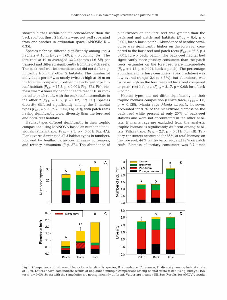
Species richness differed significantly among the 3habitats at 10 m (F2,44 = 5.69, p = 0.006; Fig. 3A). Thefore reef at 10 m averaged 32.2 species (1.6 SE) pertransect and differed significantly from the patch reefs.The back reef was intermediate and did not differ sig-nificantly from the other 2 habitats. The number ofindividuals per m2 was nearly twice as high at 10 m onthe fore reef compared to either the back-reef or patch-reef habitats (F2,44 = 15.3, p < 0.001; Fig. 3B). Fish bio-mass was 2.4 times higher on the fore reef at 10 m com-pared to patch reefs, with the back reef intermediate tothe other 2 (F2,44 = 4.02, p = 0.02; Fig. 3C). Speciesdiversity differed significantly among the 3 habitattypes (F2,44 = 5.90, p = 0.005; Fig. 3D), with patch reefshaving significantly lower diversity than the fore-reefand back-reef habitats.

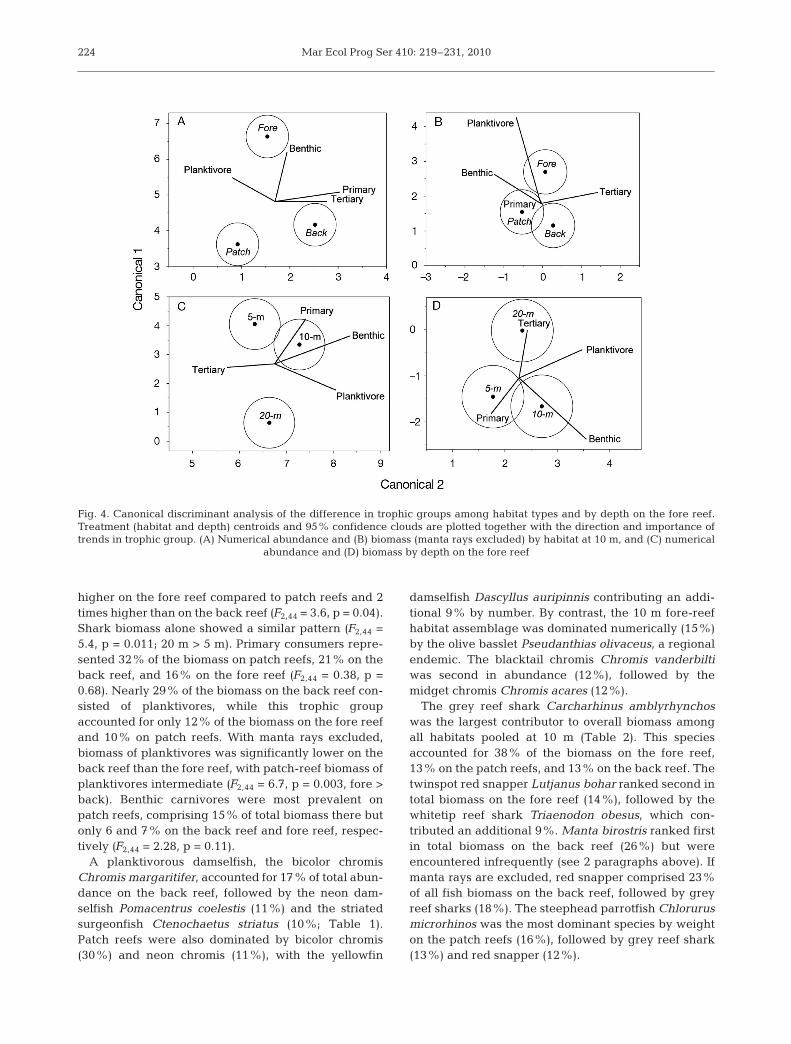
Habitat types differed significantly in their trophiccomposition using MANOVA based on number of indi-viduals (Pillai’s trace, F8,80 = 9.3, p < 0.001; Fig. 4A).Planktivores dominated all 3 habitat types in numbers,followed by benthic carnivores, primary consumers,and tertiary consumers (Fig. 3B). The abundance of

planktivores on the fore reef was greater than theback-reef and patch-reef habitats (F2,44 = 8.4, p <0.001, fore > back, patch). Abundance of benthic carni-vores was significantly higher on the fore reef com-pared to the back reef and patch reefs (F2,44 = 36.2, p <0.001, fore > back, patch). The back-reef habitat hadsignificantly more primary consumers than the patchreefs; estimates on the fore reef were intermediate(F2,44 = 4.42, p = 0.021, back > patch). The percentageabundance of tertiary consumers (apex predators) waslow overall (range: 2.4 to 4.3%), but abundance wastwice as high on the fore reef and back reef comparedto patch-reef habitats (F2,44 = 3.17, p = 0.05; fore, back> patch).

Habitat types did not differ significantly in theirtrophic biomass composition (Pillai’s trace, F8,80 = 1.6,p = 0.128). Manta rays Manta birostris, however,accounted for 91% of the planktivore biomass on theback reef while present at only 25% of back-reefstations and were not encountered in the other habi-tats. If manta rays are excluded from the analysis,trophic biomass is significantly different among habi-tats (Pillai’s trace, F8,80 = 2.7, p = 0.011; Fig. 4B). Ter-tiary consumers accounted for 65% of total biomass onthe fore reef, 44% on the back reef, and 42% on patchreefs. Biomass of tertiary consumers was 3.7 times

223

Fig. 3. Comparisons of fish assemblage characteristics (A: species, B: abundance, C: biomass, D: diversity) among habitat strataat 10 m. Letters above bars indicate results of unplanned multiple comparisons among habitat strata tested using Tukey’s HSDtests (α = 0.05). Strata with the same letter are not significantly different. Values are means +SE. See ‘Results’ for ANOVA results

Mar Ecol Prog Ser 410: 219–231, 2010

higher on the fore reef compared to patch reefs and 2times higher than on the back reef (F2,44 = 3.6, p = 0.04).Shark biomass alone showed a similar pattern (F2,44 =5.4, p = 0.011; 20 m > 5 m). Primary consumers repre-sented 32% of the biomass on patch reefs, 21% on theback reef, and 16% on the fore reef (F2,44 = 0.38, p =0.68). Nearly 29% of the biomass on the back reef con-sisted of planktivores, while this trophic groupaccounted for only 12% of the biomass on the fore reefand 10% on patch reefs. With manta rays excluded,biomass of planktivores was significantly lower on theback reef than the fore reef, with patch-reef biomass ofplanktivores intermediate (F2,44 = 6.7, p = 0.003, fore >back). Benthic carnivores were most prevalent onpatch reefs, comprising 15% of total biomass there butonly 6 and 7% on the back reef and fore reef, respec-tively (F2,44 = 2.28, p = 0.11).

A planktivorous damselfish, the bicolor chromisChromis margaritifer, accounted for 17% of total abun-dance on the back reef, followed by the neon dam-selfish Pomacentrus coelestis (11%) and the striatedsurgeonfish Ctenochaetus striatus (10%; Table 1).Patch reefs were also dominated by bicolor chromis(30%) and neon chromis (11%), with the yellowfin

damselfish Dascyllus auripinnis contributing an addi-tional 9% by number. By contrast, the 10 m fore-reefhabitat assemblage was dominated numerically (15%)by the olive basslet Pseudanthias olivaceus, a regionalendemic. The blacktail chromis Chromis vanderbiltiwas second in abundance (12%), followed by themidget chromis Chromis acares (12%).

The grey reef shark Carcharhinus amblyrhynchoswas the largest contributor to overall biomass amongall habitats pooled at 10 m (Table 2). This speciesaccounted for 38% of the biomass on the fore reef,13% on the patch reefs, and 13% on the back reef. Thetwinspot red snapper Lutjanus bohar ranked second intotal biomass on the fore reef (14%), followed by thewhitetip reef shark Triaenodon obesus, which con-tributed an additional 9%. Manta birostris ranked firstin total biomass on the back reef (26%) but wereencountered infrequently (see 2 paragraphs above). Ifmanta rays are excluded, red snapper comprised 23%of all fish biomass on the back reef, followed by greyreef sharks (18%). The steephead parrotfish Chlorurusmicrorhinos was the most dominant species by weighton the patch reefs (16%), followed by grey reef shark(13%) and red snapper (12%).

224

Fig. 4. Canonical discriminant analysis of the difference in trophic groups among habitat types and by depth on the fore reef.Treatment (habitat and depth) centroids and 95% confidence clouds are plotted together with the direction and importance oftrends in trophic group. (A) Numerical abundance and (B) biomass (manta rays excluded) by habitat at 10 m, and (C) numerical

abundance and (D) biomass by depth on the fore reef

Friedlander et al.: Fish assemblage structure at a pristine atoll

Comparisons among depths on the fore reef

The assemblage structure of fishes based on abun-dance formed distinct clusters in ordination spaceamong depth strata on the fore reef (Global R = 0.61,Stress = 0.10; Fig. 2B). The 5 m and 20 m depth strataformed distinct clusters that were well separated inordination space (ANOSIM R = 0.94). The fish assem-blage at 10 m overlapped with both the 5 m assem-blage (ANOSIM R = 0.43) and the 20 m assemblage(ANOSIM R = 0.50).

Species richness differed among the 3 fore-reefdepth strata (F2,44 = 10.6, p < 0.001; Fig. 5A). The low-est species richness was found at the 5 m stratum (27.7[0.8 SE]), followed by the 10 m (32.2 [0.8 SE]) and 20 mstrata (34.4 [1.0 SE]). Numbers per m2 at 20 m weremore than twice as high as those at 5 m and 1.5 timeshigher than at 10 m (F2,44 = 29.5, p < 0.001; Fig. 5B).Fish biomass at 20 m on the fore reef was 1.8 timeshigher than the 5 m depth stratum and 1.3 timesgreater than the 10 m stratum. Biomass at 20 m wassignificantly greater than at 5 m, with 10 m being inter-mediate (F2,44 = 3.6, p = 0.04; Fig. 5C). Diversity washighest at the 10 m depth, followed by the 5 m stratum,with diversity in the 20 m stratum significantly lowerthan the other 2 (F2,44 = 10.3, p < 0.001; Fig. 5D).

Depth strata differed significantly in their trophic com-position using MANOVA based on number of individu-als (Pillai’s trace, F8,80 = 7.3, p < 0.001; Fig. 4C). Plankti-

vores accounted for 43% of numerical abundance at 5 m,58% at 10 m, and 81% at 20 m. These fishes were 4.0times and 2.2 times more numerous at 20 m versus 5 mand 10 m, respectively (F2,44 = 40.0, p < 0.001, 20 m >10 m > 5 m). Benthic carnivores were the next most nu-merous trophic group and were statistically indistin-guishable between 5 and 10 m, each of which was signif-icantly higher than at 20 m (F2,44 = 15.9, p < 0.001, 20 m >10 m, 5 m). The percentage abundance of primary con-sumers ranged from 5% at 20 m to 18% at 5 m and wassignificantly lower at 20 m compared to the 2 shallowerdepth strata (F2,44 = 14.6, p < 0.001, 20 m > 10 m, 5 m).Tertiary consumer abundance did not significantly differamong depths (F2,44 = 2.4, p = 0.11) and ranged from 2%at 20 m to 3% at 5 m (Fig. 5B).

Trophic composition differed significantly amongdepth strata based on biomass (Pillai’s trace, F8,80 = 3.3,p = 0.002; Fig. 4D). Tertiary consumer biomass, as apercentage of the total, ranged from 61% at 5 m to77% at 20 m (Fig. 5C). Biomass of tertiary consumerswas 2.2 times higher at 20 m compared to 5 m and 1.5times higher than at 10 m (F2,44 = 4.17, p = 0.03; 20 m >5 m). This pattern also held true when only sharkswere considered (F2,44 = 3.9, p = 0.027; 20 m > 5 m). Pri-mary consumer biomass ranged from 8% of total bio-mass at 20 m to 24% at 5 m (F2,44 = 3.3, p = 0.05; 5 m =10 m > 20 m). Benthic carnivores comprised 4% of totalbiomass at 20 m, 7% at 10 m, and 8% at 5 m, with bio-mass at 10 m significantly higher than the 20 m stratum

225

Patch reef Back reef Fore reefSpecies Abundance Rep. Species Abundance Rep. Species Abundance Rep.

Chromis 0.40 ± 0.07 30.1 Chromis 0.23 ± 0.05 16.9 Pseudanthias 0.37 ± 0.11 14.7margaritifer margaritifer olivaceus

Pomacentrus 0.15 ± 0.09 11.4 Pomacentrus 0.15 ± 0.05 11.0 Chromis 0.30 ± 0.06 12.1coelestis coelestis vanderbilti

Dascyllus 0.11 ± 0.02 8.6 Ctenochaetus 0.14 ± 0.03 10.2 Chromis 0.30 ± 0.07 12.0auripinnis striatus acares

Caesio 0.05 ± 0.02 3.6 Siphamia 0.08 ± 0.09 5.6 Chromis 0.23 ± 0.04 9.1teres versicolor margaritifer

Acanthurus 0.05 ± 0.01 3.6 Acanthurus 0.07 ± 0.01 4.8 Thalassoma 0.16 ± 0.03 6.4nigricans nigricans quinquevittatum

Ctenochaetus 0.05 ± 0.01 3.5 Dascyllus 0.07 ± 0.02 4.7 Plectroglyphidodon 0.10 ± 0.01 4.0striatus auripinnis johnstonianus

Ctenochaetus 0.05 ± 0.01 3.4 Eviota 0.06 ± 0.02 4.5 Acanthurus 0.10 ± 0.01 3.9cyanocheilus albolineata nigricans

Eviota 0.04 ± 0.02 3.2 Chromis 0.06 ± 0.01 4.0 Paracirrhites 0.09 ± 0.01 3.5albolineata xanthura arcatus

Thalassoma 0.03 ± 0.01 2.0 Ctenochaetus 0.04 ± 0.01 3.0 Ctenochaetus 0.08 ± 0.01 3.4lutescens cyanocheilus cyanocheilus

Gomphosus 0.03 ± 0.01 2.0 Thalassoma 0.03 ± 0.01 2.5 Cirrhilabrus 0.08 ± 0.05 3.3varius lutescens exquisitus

Table 1. Numerical abundance of top 10 species in each habitat at 10 m. Species ordered by overall percentage representation in habitats (Rep., %). Abundance = ind. m–2, mean ± SE

Mar Ecol Prog Ser 410: 219–231, 2010226

Patch reef Back reef Fore reefSpecies Biomass Rep. Species Biomass Rep. Species Biomass Rep.

Chlorurus 0.15 ± 0.03 16.2 Manta 0.45 ± 0.21 26.4 Carcharhinus 0.88 ± 0.37 37.8microrhinos birostris amblyrhynchos

Carcharhinus 0.12 ± 0.09 12.7 Lutjanus 0.29 ± 0.06 17.0 Lutjanus 0.32 ± 0.08 13.9amblyrhynchos bohar bohar

Lutjanus 0.11 ± 0.02 11.6 Carcharhinus 0.22 ± 0.09 12.7 Triaenodon 0.22 ± 0.11 9.5bohar amblyrhynchos obesus

Triaenodon 0.10 ± 0.03 10.8 Triaenodon 0.10 ± 0.05 6.2 Caesio 0.11 ± 0.08 4.8obesus obesus teres

Monotaxis 0.07 ± 0.03 7.8 Ctenochaetus 0.09 ± 0.02 5.5 Chlorurus 0.09 ± 0.02 3.9grandoculis striatus microrhinos

Caesio 0.05 ± 0.02 5.6 Chlorurus 0.08 ± 0.02 4.6 Acanthurus 0.09 ± 0.01 3.8teres microrhinos nigricans

Ctenochaetus 0.03 ± 0.01 3.7 Acanthurus 0.05 ± 0.01 3.1 Ctenochaetus 0.08 ± 0.01 3.5striatus nigricans cyanocheilus

Acanthurus 0.03 ± 0.01 3.0 Lutjanus 0.04 ± 0.03 2.5 Monotaxis 0.05 ± 0.02 2.3nigricans gibbus grandoculis

Ctenochaetus 0.02 ± 0.01 2.3 Caranx 0.03 ± 0.02 1.8 Melichthys 0.05 ± 0.02 2.0cyanocheilus melampygus niger

Lutjanus 0.02 ± 0.01 2.2 Cephalopholis 0.03 ± 0.01 1.7 Cephalopholis 0.03 ± 0.01 1.4gibbus argus argus

Table 2. Biomass of top 10 species in each habitat at 10 m. Species ordered by overall percentage representation in habitats(Rep., %). Biomass = t ha–1, mean ± SE

Fig. 5. Comparisons of fish assemblage characteristics (A: species, B: abundance, C: biomass, D: diversity) among depth strata onthe fore reef. Letters above bars indicate results of unplanned multiple comparisons among depth strata tested using Tukey’sHSD tests (α = 0.05). Strata with the same letter are not significantly different. Values are means +SE. See ‘Results’ for

ANOVA results

Friedlander et al.: Fish assemblage structure at a pristine atoll

and the 5 m stratum being intermediate (F2,44 = 3.9, p =0.03). Planktivore biomass increased monotonicallywith depth, although these differences were not statis-tically significant (F2,44 = 2.5, p = 0.09).

At 10 and 20 m, the olive basslet was the most impor-tant species by number, accounting for 15% and 39%of total abundance in these fore-reef depth strata,respectively (Table 3). This species occurred in lowabundance at 5 m fore-reef sites and only accountedfor 0.02% of total numbers at this depth. The bicolorchromis ranked second in overall numbers at 20 m andfourth at 10 m, accounting for 22% and 9% of the totalat these depths, respectively. At 5 m, the blacktailchromis was numerically dominant and accounted for31% of the total by number at this depth, followed bythe fivestripe wrasse Thalassoma quinquevittatumwith 17% and the herbivorous damselfish Plectro-glyphidodon dickii with 5%.

Grey reef shark and red snapper were the first- andsecond-ranked species by weight, respectively, amongall 3 depth strata on the fore reef (Table 4). The contri-bution of Carcharhinus amblyrhynchos ranged from38% at 5 m and 10 m to 56% at 20 m. Lutjanus boharbiomass ranged from 10% at 20 m to 16% at 5 m. Atboth 10 and 20 m, Triaenodon obesus was third in totalbiomass with contributions of 9% at each, respectively.At 5 m depth, a triggerfish, the omnivorous black dur-gon Melichthys niger, ranked third and represented5% of total fish biomass.

Prey size structure

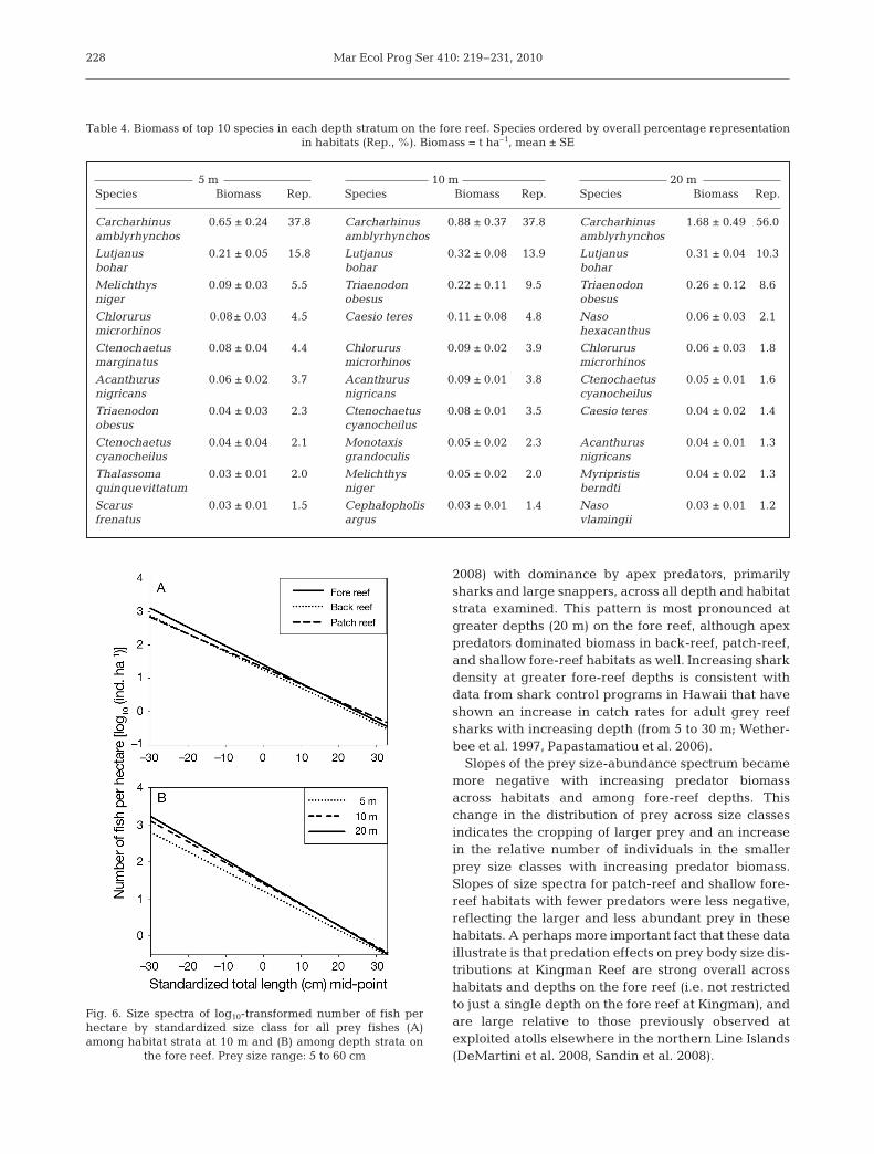
Regressions of size-specific numerical densities of allprey taxa on body length class showed an interactionbetween size class and habitat type (ANCOVA F2,29 =4.38, p = 0.02; Fig. 6A). The slope of the patch-reefregression was significantly different (less negative)than the slopes of the back-reef and fore-reef regres-sions (both p < 0.05). Slopes among habitats becameincreasingly more negative from patch reef (–0.054) toback reef (–0.064) to fore reef (–0.066, p < 0.05). On thefore reef, there was an interaction between size classand depth (ANCOVA F2,29 = 3.2, p = 0.05; Fig. 6B). Theslope of the 20 m regression was the most negative anddiffered significantly from the 10 m regression (10 m[–0.062] < 20 m [–0.070], p < 0.05). The 5 m (–0.066)and 20 m slopes did not differ significantly, nor did the10 m and 5 m slopes (both p > 0.05).

DISCUSSION

Structural patterns of the undisturbed fish assem-blage at Kingman are a baseline that reflects naturalecological processes that are not influenced by fishingor other anthropogenic factors.

The most striking feature of this assemblage is the in-verted biomass pyramid (with more predator than preybiomass, sensu DeMartini et al. 2008 and Sandin et al.

227

5 m 10 m 20 mSpecies Abundance Rep. Species Abundance Rep. Species Abundance Rep.

Chromis 0.59 ± 0.09 31.5 Pseudanthias 0.37 ± 0.11 14.7 Pseudanthias 1.52 ± 0.32 39.5vanderbilti olivaceus olivaceus

Thalassoma 0.32 ± 0.03 17.0 Chromis 0.30 ± 0.06 12.1 Chromis 0.86 ± 0.14 22.3quinquevittatum vanderbilti margaritifer

Plectroglyphidodon 0.09 ± 0.01 4.6 Chromis 0.30 ± 0.07 12.0 Chromis 0.42 ± 0.10 10.8dickii acares acares

Stegastes 0.08 ± 0.01 4.1 Chromis 0.23 ± 0.04 9.1 Chromis 0.06 ± 0.02 1.7aureus margaritifer xanthura

Acanthurus 0.07 ± 0.02 3.9 Thalassoma 0.16 ± 0.03 6.4 Ctenochaetus 0.06 ± 0.01 1.5nigricans quinquevittatum cyanocheilus

Chromis 0.07 ± 0.03 3.8 Plectroglyphidodon 0.10 ± 0.01 4.0 Labroides 0.06 ± 0.01 1.5margaritifer johnstonianus dimidiatus

Ctenochaetus 0.06 ± 0.03 3.2 Acanthurus 0.10 ± 0.01 3.9 Halichoeres 0.06 ± 0.01 1.4marginatus nigricans ornatissimus

Plectroglyphidodon 0.05 ± 0.02 3.1 Paracirrhites 0.09 ± 0.01 3.5 Cirrhilabrus 0.05 ± 0.02 1.4johnstonianus arcatus exquisitus

Ctenochaetus 0.04 ± 0.01 2.4 Ctenochaetus 0.09 ± 0.04 3.4 Paracirrhites 0.05 ± 0.01 1.4cyanocheilus cyanocheilus arcatus

Melichthys 0.04 ± 0.01 2.0 Cirrhilabrus 0.08 ± 0.05 3.3 Plectroglyphidodon 0.05 ± 0.01 1.3niger exquisitus johnstonianus

Table 3. Numerical abundance of top 10 species in each depth stratum on the fore reef. Species ordered by overall percentage representation in habitats (Rep., %). Abundance = ind. m–2, mean ± SE

Mar Ecol Prog Ser 410: 219–231, 2010

2008) with dominance by apex predators, primarilysharks and large snappers, across all depth and habitatstrata examined. This pattern is most pronounced atgreater depths (20 m) on the fore reef, although apexpredators dominated biomass in back-reef, patch-reef,and shallow fore-reef habitats as well. Increasing sharkdensity at greater fore-reef depths is consistent withdata from shark control programs in Hawaii that haveshown an increase in catch rates for adult grey reefsharks with increasing depth (from 5 to 30 m; Wether-bee et al. 1997, Papastamatiou et al. 2006).

Slopes of the prey size-abundance spectrum becamemore negative with increasing predator biomassacross habitats and among fore-reef depths. Thischange in the distribution of prey across size classesindicates the cropping of larger prey and an increasein the relative number of individuals in the smallerprey size classes with increasing predator biomass.Slopes of size spectra for patch-reef and shallow fore-reef habitats with fewer predators were less negative,reflecting the larger and less abundant prey in thesehabitats. A perhaps more important fact that these dataillustrate is that predation effects on prey body size dis-tributions at Kingman Reef are strong overall acrosshabitats and depths on the fore reef (i.e. not restrictedto just a single depth on the fore reef at Kingman), andare large relative to those previously observed atexploited atolls elsewhere in the northern Line Islands(DeMartini et al. 2008, Sandin et al. 2008).

228

5 m 10 m 20 mSpecies Biomass Rep. Species Biomass Rep. Species Biomass Rep.

Carcharhinus 0.65 ± 0.24 37.8 Carcharhinus 0.88 ± 0.37 37.8 Carcharhinus 1.68 ± 0.49 56.0amblyrhynchos amblyrhynchos amblyrhynchos

Lutjanus 0.21 ± 0.05 15.8 Lutjanus 0.32 ± 0.08 13.9 Lutjanus 0.31 ± 0.04 10.3bohar bohar bohar

Melichthys 0.09 ± 0.03 5.5 Triaenodon 0.22 ± 0.11 9.5 Triaenodon 0.26 ± 0.12 8.6niger obesus obesus

Chlorurus 0.08± 0.03 4.5 Caesio teres 0.11 ± 0.08 4.8 Naso 0.06 ± 0.03 2.1microrhinos hexacanthus

Ctenochaetus 0.08 ± 0.04 4.4 Chlorurus 0.09 ± 0.02 3.9 Chlorurus 0.06 ± 0.03 1.8marginatus microrhinos microrhinos

Acanthurus 0.06 ± 0.02 3.7 Acanthurus 0.09 ± 0.01 3.8 Ctenochaetus 0.05 ± 0.01 1.6nigricans nigricans cyanocheilus

Triaenodon 0.04 ± 0.03 2.3 Ctenochaetus 0.08 ± 0.01 3.5 Caesio teres 0.04 ± 0.02 1.4obesus cyanocheilus

Ctenochaetus 0.04 ± 0.04 2.1 Monotaxis 0.05 ± 0.02 2.3 Acanthurus 0.04 ± 0.01 1.3cyanocheilus grandoculis nigricans

Thalassoma 0.03 ± 0.01 2.0 Melichthys 0.05 ± 0.02 2.0 Myripristis 0.04 ± 0.02 1.3quinquevittatum niger berndti

Scarus 0.03 ± 0.01 1.5 Cephalopholis 0.03 ± 0.01 1.4 Naso 0.03 ± 0.01 1.2frenatus argus vlamingii

Table 4. Biomass of top 10 species in each depth stratum on the fore reef. Species ordered by overall percentage representation in habitats (Rep., %). Biomass = t ha–1, mean ± SE

Fig. 6. Size spectra of log10-transformed number of fish perhectare by standardized size class for all prey fishes (A)among habitat strata at 10 m and (B) among depth strata on

the fore reef. Prey size range: 5 to 60 cm

Friedlander et al.: Fish assemblage structure at a pristine atoll

Fishes from lower trophic levels in general showedpredictable patterns consistent with more typicalfished areas. Abundance and biomass increased withproximity to the pelagic environment (from patch reefsto back reef to fore reef) and with increasing depth onthe fore reef. Planktivores numerically dominated allhabitats and depths, largely driving the trends in totalabundance. Species density and diversity showed sim-ilar patterns across habitats, with the exception of adisproportionately lower diversity at 20 m depth on thefore reef. The fish assemblage in this stratum was dom-inated numerically by 1 species of planktivore, thecentral Pacific endemic Pseudanthias olivaceus. Ingeneral, the planktivore guild was the largest contrib-utor to diversity, while benthic carnivores composedthe largest proportion of total species across strata.Herbivores showed highest density and biomass on thefore reef, although they were least abundant at thedeepest (20 m) stratum. Conversely, benthic carnivoreabundance increased at greater depths, reflecting thegreater abundance of small wrasses (Labridae) withdepth.

Many studies, dating back to the 1960s, have exam-ined the spatial distribution of fishes on coral reefs (Hi-att & Strasburg 1960, Goldman & Talbot 1976, Russ1984, Williams 1991). Prominent factors affecting thesize and composition of reef fish assemblages includephysical characteristics (e.g. depth, wave exposure), re-source availability (e.g. food, shelter), and interspecificinteractions (e.g. predation, competition). While manyassemblage changes generally apply across fish taxa,others are more specific to particular trophic guilds.

Two gradients have received particular attention intheir effects on tropical reef fish assemblage structure:depth and proximity to the pelagic environment. Manycharacteristics of fish assemblages (richness, numeri-cal abundance, biomass) have been shown to changeconsistently with depth (from the surface to about30 m) and can be attributed to the closer proximity tohabitats with greatly different physical and biologicaldiversity (Gosline 1965, Friedlander & Parrish 1998,Brokovich et al. 2008). Planktivores and herbivoresappear to respond particularly strongly to depth gradi-ents. In particular, planktivore density commonly in-creases with depth on the fore reef as a result of theproximity to reef edges that provide higher concentra-tions of plankton (Hobson & Chess 1978, Thresher &Colin 1986). Conversely, herbivores tend to decreasein density with depth, likely responding to lesser avail-ability, productivity, and/or quality of algal resourcesat greater depths (Russ 1984, Fox & Bellwood 2007).

Similarly, proximity to the pelagic environment hasbeen shown to predictably alter the structure of reeffish assemblages. Patch reefs and back-reef habitatsoften have smaller areal extents, lower habitat diver-

sity, and lower structural complexity relative to adja-cent fore-reef habitats (Parrish 1989). As such, numer-ical density and species diversity tend to increase frominshore patch or lagoonal habitats toward outer reefslope and fore-reef habitats (Galzin 1987, Lecchini etal. 2003, Alvarez-Filip et al. 2006).

The present study demonstrates that spatial patternsof distribution among habitats and depths can be con-sistent between fished and unfished reefs yet obscuresome fundamental differences resulting from extrac-tion. Several general and readily demonstrable simi-larities between fished and unfished reefs (depth andhabitat predilections of herbivores and planktivores)are static characteristics that reflect fundamental pro-cesses of photosynthesis and ocean currents andplankton transport. Gross patterns of similarity be-tween fished and unfished reefs in relative trophiclevel abundance and biomass distributions amonghabitats and depths gloss over the fundamental factthat, on fished reefs, size structure and abundance-to-biomass relationships are shifted among trophic levelsat depth and within particular habitats. Our observa-tions clearly show that the extraction of apex predatorsthat results in meaningful biomass shifts amongtrophic levels within habitats on reefs does not neces-sarily result in changes in the spatial (among habitatand across-depth) distribution of biomass for particularguilds and trophic levels.

Impressions of similarity based on static properties ofabundance and biomass distributions, however, over-look the less obvious and more difficult to demonstratedynamic properties of fish assemblages. These includethe species-specific age and size distributions andgrowth and mortality rates that are undoubtedly im-portant for resource production and sustainable fish-eries management. Regardless of whether overextrac-tion results in the ‘fishing down’ (Pauly et al. 1998) orthe ‘fishing through’ (Essington et al. 2006) of foodwebs, it is clear that the dynamic properties of resourcespecies populations are key to understanding andmanaging their sustainable use.

Apex predators clearly exert a strong top-down con-trol on the entire ecosystem (DeMartini et al. 2005,Sandin et al. 2008), yet these species are the most vul-nerable to exploitation (Myers & Worm 2003). Theremoval of these species can lead to reefs that aredominated by small-bodied, lower trophic-level spe-cies that do not represent the natural state and maygive a false impression of true ecological processes(Friedlander & DeMartini 2002, DeMartini et al. 2008).This shifting baseline syndrome (Pauly 1995, Sheppard1995) plagues most contemporary studies on coralreefs and the results of our work will help set a base-line for comparisons with reefs under varying degreesof human disturbance.

229

Mar Ecol Prog Ser 410: 219–231, 2010

Remote, uninhabited locations represent some ofthe last remaining ‘pristine’ coral reefs left on earthand give us a window into the past as to what reefslooked like prior to human extraction (Knowlton &Jackson 2008). These few remaining large-scale,intact, predator-dominated reef ecosystems offer achance to examine what could occur if larger, more ef-fective, no-take marine protected areas (MPAs) wereimplemented elsewhere. The creation of large MPAsthat protect entire ecosystems like the northwesternHawaiian Islands, Great Barrier Reef, Phoenix Islands,and US Pacific Remote Islands offer a tremendousopportunity to conserve the remaining intact coralreefs and avoid the pitfall of further promulgating theshifting baseline.

Acknowledgements. We thank the captain and crew of theMV ‘Searcher’ for logistical support and hospitality. The USFish and Wildlife Service granted permission to operate in theKingman Atoll National Wildlife Refuge. This study was madepossible thanks to the generous support of the National Geo-graphic Society, the Moore Family Foundation, The Fair-weather Foundation, The Medical Foundation for the Study ofthe Environment, Ed Scripps, John Rowe, and another privatedonor. Financial support was also provided by NOAA Fish-eries, Office of Habitat Conservation, Coral Reef Conserva-tion Program (to E.E.D.).

LITERATURE CITED

Alvarez-Filip L, Reyes-Bonilla H, Calderon-Aguilera L (2006)Community structure of fishes in Cabo Pulmo Reef, Gulf ofCalifornia. PSZN I: Mar Ecol 27:253–262

Bellwood DR, Hughes TP, Folke C, Nystrom M (2004) Con-fronting the coral reef crisis. Nature 429:827–833

Birkeland C (2004) Ratcheting down the coral reefs. Bio-science 54:1021–1027

Brokovich E, Einbinder S, Shashar N, Kiflawi M, Kark S(2008) Descending to the twilight-zone: changes in coralreef fish assemblages along a gradient down to 65 m. MarEcol Prog Ser 371:253–262

Charles C, Sandin S (2009) Line Islands. In: Gillespie RG,Clague D (eds) Encyclopedia of islands. University of Cal-ifornia Press, Berkeley, CA, p 553–558

Clarke KR, Gorley RN (2006) PRIMER v6: user manual/tutor-ial. PRIMER-E, Plymouth

DeMartini EE, Friedlander AM, Holzwarth SR (2005) Size atsex change in protogynous labroids, prey size distribu-tions, and apex predator densities at NW Hawaiian atolls.Mar Ecol Prog Ser 297:259–271

DeMartini EE, Friedlander AM, Sandin SA, Sala E (2008) Dif-ferences in fish assemblage structure between fished andunfished atolls in the northern Line Islands, central Pacific.Mar Ecol Prog Ser 365:199–215

Dulvy NK, Polunin NVC, Mill AC, Graham NAJ (2004) Sizestructural change in lightly exploited coral reef fish com-munities: evidence for weak indirect effects. Can J FishAquat Sci 61:466–475

Essington TE, Beadreau AH, Wiedenmann J (2006) Fishingthrough marine food webs. Proc Natl Acad Sci USA 103:3171–3175

Fox RJ, Bellwood DR (2007) Quantifying herbivory across a

coral reef depth gradient. Mar Ecol Prog Ser 339:49–59Friedlander AM, DeMartini EE (2002) Contrasts in density,

size, and biomass of reef fishes between the northwesternand the main Hawaiian Islands: the effects of fishing downapex predators. Mar Ecol Prog Ser 230:253–264

Friedlander AM, Parrish JD (1998) Habitat characteristicsaffecting fish assemblages on a Hawaiian coral reef. J ExpMar Biol Ecol 224:1–30

Galzin R (1987) Structure of fish communities of French Poly-nesian coral reefs. I. Spatial scales. Mar Ecol Prog Ser 41:129–136

Goldman B, Talbot FH (1976) Aspects of the ecology of coralreef fishes. In: Jones OA, Endean R (eds) Biology and geol-ogy of coral reefs, Vol 3. Academic Press, New York, NY,p 125–154

Gosline WA (1965) Vertical zonation of inshore fishes in theupper water layers of the Hawaiian Islands. Ecology 46:823–831

Graham NAJ, Dulvy NK, Jennings S, Polunin NVC (2005)Size-spectra as indicators of the effects of fishing on coralreef fish assemblages. Coral Reefs 24:118–124

Green RH (1979) Sampling design and statistical methods forenvironmental biologists. Wiley Interscience, New York,NY

Harmelin-Vivien ML (2002) Energetics and fish diversity oncoral reefs. In: Sale P (ed) Coral reef fishes: dynamics anddiversity in a complex ecosystem. Academic Press, SanDiego, CA, p 265–274

Hiatt RW, Strasburg DW (1960) Ecological relationships of thefish fauna on coral reefs of the Marshall Islands. EcolMonogr 30:65–127

Hobson ES, Chess JR (1978) Trophic relationships amongfishes and plankton in the lagoon at Enewetok atoll, Mar-shall Islands. Fish Bull 76:133–153

Jackson JBC, Kirby MX, Berger WH, Bjorndal KA and others(2001) Historical overfishing and the recent collapse ofcoastal ecosystems. Science 293:629–638

Jennings S, Kaiser MJ (1998) The effects of fishing on marineecosystems. Adv Mar Biol 34:201–352

Jennings S, Polunin NVC (1996) Effects of fishing effort andcatch rates upon the structure and biomass of Fijian reeffish communities. J Appl Ecol 33:400–412

Kleinbaum DG, Kupper LL (1978) Applied regression analysisand other multivariable methods. Duxbury Press, NorthScituate, MA

Knowlton N, Jackson JBC (2008) Shifting baselines, localimpacts, and global change on coral reefs. PLoS Biol 6:e54

Kulbicki M, Guillemot N, Amand M (2005) A generalapproach to length–weight relationships for New Cale-donian lagoon fishes. Cybium 29:235–252

Lecchini D, Adjeroud M, Pratchett MS, Cadoret L, Galzin R(2003) Spatial structure of coral reef fish communities inthe Ryuku Islands, southern Japan. Oceanol Acta 26:537–547

Letourneur Y (1998) Length-weight relationship of somemarine fish species in Reunion Island, New Caledonia.Naga ICLARM Q 21:39–46

Ludwig JA, Reynolds JF (1988) Statistical ecology. John Wiley& Sons, New York, NY

Mapstone BD, Ayling AM (1998) An investigation of the opti-mum methods and unit sizes or the visual estimation ofabundance of some coral reef organisms. Great BarrierReef Mar Park Auth Res Publ No. 47, Townsville, QLD

Maragos J, Friedlander AM, Godwin S, Musburger C andothers (2008) US coral reefs in the Line and PhoenixIslands, central Pacific Ocean: status, threats, and signifi-cance. Biology and paleoceanography of the coral reefs in

230

Friedlander et al.: Fish assemblage structure at a pristine atoll

the northwestern Hawaiian Islands. In: Riegl B, Dodge R(eds) Coral reefs of the United States. Springer-Verlag,Dordrecht, p 643–655

McClanahan TR, Graham NAJ, Calnan JM, MacNeil MA (2007)Toward pristine biomass: reef fish recovery in coral reefmarine protected areas in Kenya. Ecol Appl 17:1055–1067

Myers RA, Worm B (2003) Rapid worldwide depletion ofpredatory fish communities. Nature 423:280–283

Pandolfi JM, Jackson JBC, Baron N, Bradbury RH and others(2005) Are US coral reefs on the slippery slope to slime?Science 307:1725–1726

Papastamatiou YP, Wetherbee BM, Lowe CG, Crow GL (2006)Distribution and diet of four species of carcharhinid sharkin the Hawaiian Islands: evidence for resource partition-ing and competitive exclusion. Mar Ecol Prog Ser 320:239–251

Parrish JD (1989) Fish communities of interacting shallow-water habitats in tropical oceanic regions. Mar Ecol ProgSer 58:143–160

Pauly D (1995) Anecdotes and the shifting baseline syndromeof fisheries. Trends Ecol Evol 10:430

Pauly D, Christensen V, Dalsgaaard J, Froese R, Torres F Jr(1998) Fishing down marine food webs. Science 279:860–863

Rochet MJ, Trenkel VM (2003) Which community indicatorscan measure the impact of fishing? A review and propos-als. Can J Fish Aquat Sci 60:86–99

Russ G (1984) Distribution and abundance of herbivorous

fishes in the central Great Barrier Reef. I. Levels of vari-ability across the entire continental shelf. Mar Ecol ProgSer 20:23–34

Russ GR, Alcala AC (1996) Marine reserves-rates and pat-terns of recovery and decline of large predatory fish. EcolAppl 6:947–961

Sandin SA, Smith JE, DeMartini EE, Dinsdale EA and others(2008) Baselines and degradation of coral reefs in thenorthern Line Islands. PLoS ONE 3(2):e1548 doi:10.1371/journal.pone.0001548

Sheppard C (1995) The shifting baseline syndrome. Mar Pol-lut Bull 30:766–767

Stevenson C, Katz LS, Micheli F, Block B and others (2007)High apex predator biomass on remote Pacific islands.Coral Reefs 26:47–51

Thresher RE, Colin PL (1986) Trophic structure, diversity andabundance of fishes of the deep reef (30-300 m) at Enewe-tak, Marshall Islands. Bull Mar Sci 38:410–426

Wetherbee BM, Crow GL, Lowe CG (1997) Distribution,reproduction and diet of the gray reef shark Carcharhi-nus amblyrhynchos in Hawaii. Mar Ecol Prog Ser 151:181–189

Williams DMcB (1991) Patterns and processes in the distribu-tion of coral reef fishes. In: Sale PF (ed) The ecology offishes on coral reefs. Academic Press, San Diego, CA,p 437–474

Zar JH (1999) Biostatistical analysis, 4th edn. Prentice Hall,Upper Saddle River, NJ

231

Editorial responsibility: John Choat,Townsville, Australia

Submitted: June 30, 2009; Accepted: April 20, 2010Proofs received from author(s): June 26, 2010