spatial relationships among soil nutrients, plant ...spatial relationships among soil nutrients,...
TRANSCRIPT
Spatial Relationships among Soil Nutrients,
Plant Biodiversity and Aboveground Biomass
in the Inner Mongolia Grassland, China
by
Fei Yuan
A Thesis Presented in Partial Fulfillment of the Requirements for the Degree
Master of Science
Approved June 2011 by the Graduate Supervisory Committee:
Jianguo (Jingle) Wu, Chair
Helen I. Rowe Andrew T. Smith
ARIZONA STATE UNIVERSITY
August 2011
i
ABSTRACT
The relationship between biodiversity and ecosystem functioning (BEF) is
a central issue in ecology, and a number of recent field experimental studies have
greatly improved our understanding of this relationship. Spatial heterogeneity is a
ubiquitous characterization of ecosystem processes, and has played a significant
role in shaping BEF relationships. The first step towards understanding the
effects of spatial heterogeneity on the BEF relationships is to quantify spatial
heterogeneity characteristics of key variables of biodiversity and ecosystem
functioning, and identify the spatial relationships among these variables. The
goal of our research was to address the following research questions based on data
collected in 2005 (corresponding to the year when the initial site background
information was conducted) and in 2008 (corresponding to the year when removal
treatments were conducted) from the Inner Mongolia Grassland Removal
Experiment (IMGRE) located in northern China: 1) What are the spatial patterns
of soil nutrients, plant biodiversity, and aboveground biomass in a natural
grassland community of Inner Mongolia, China? How are they related spatially?
and 2) How do removal treatments affect the spatial patterns of soil nutrients,
plant biodiversity, and aboveground biomass? Is there any change for their spatial
correlations after removal treatments? Our results showed that variables of
biodiversity and ecosystem functioning in the natural grassland community would
present different spatial patterns, and they would be spatially correlated to each
other closely. Removal treatments had a significant effect on spatial structures
ii
and spatial correlations of variables, compared to those prior to the removal
treatments. The differences in spatial patterns of plant and soil variables and their
correlations before and after the biodiversity manipulation may not imply that the
results from BEF experiments like IMGRE are invalid. However, they do suggest
that the possible effects of spatial heterogeneity on the BEF relationships should
be critically evaluated in future studies.

iii
ACKNOWLEDGMENTS
First and foremost, I express my appreciation for the guidance and
patience provided by my advisor Dr. Jianguo Wu. He is a model advisor and
taught me many things. Without his help and support, this thesis could never
have been completed.
I would also like to thank my committee members, Dr. Helen Rowe and
Dr. Andrew Smith, for their guidance during the development of this research and
their comments on earlier draft of this document. Also, I must thank them for
agreeing on working on thesis committee in a very short notice, and giving me so
much support for completing my thesis work.
For data collection, I would like to express my appreciation to professors
and graduate students at Institute of Botany, Chinese Academy of Sciences, who
participated in the fieldwork of the IMGRE project, especially Xingguo Han,
Yongfei Bai, Jianhui Huang, Xiaotao Lv, Meng Wang, and Qiang Yu. I also
thank Ang Li for providing valuable advice for statistical analysis.
I would also like to thank all of my former and current labmates for their
encouragement and support during my graduate school years at ASU. They
include: Jeff Ackley, Alex Buyantuyev, Christopher M. Clark, Lisa Dirks, Zhibin
Jia, Cheng Li, Junxiang Li, Cunzhu Liang, Jennifer Litteral, Fengqiao Liu,
Kaesha Neil, Ronald Pope, Guixia Qian, Tracy Shoumaker, Yu Tian, Hong Xiao,
Qi Yang, Chengbo Yi, Ge Zhang, Jing Zhang, and Ting Zhou.

iv
Finally, my most emotional thanks go to my parents for their patience and
understanding of my study in the US. I could not take care of them much when I
was studying here, and I am indebted to them a lot. I love you both forever.
v
TABLE OF CONTENTS
Page
LIST OF TABLES……………………………………………………………….viii
LIST OF FIGURES……………………………………………………………….ix
CHAPTER
1 INTRODUCTION: IMPORTANCE OF SPATIAL
HETEROGENEITY IN UNDERSTANDING THE RELATIONSHIP
BETWEEN IODIVERSITY AND ECOSYSTEM
FUNCTIONING……………………………………………………..1
Introduction………………………………………………….1
The relationship between biodiversity and ecosystem functioning...3
Effects of spatial heterogeneity on the BEF relationships……….7
2 SPATIAL PATTERNS OF SOIL NUTRIENTS, PLANT DIVERSITY,
AND ABOVEGROUND BIOMASS AND THEIR RELATIONSHIPS
IN A NATURAL GRASSLAND COMMUNITY IN INNER
MONGOLIA, CHINA……………………………………………….11
Introduction……………………………………..……………….11
Materials and methods……………………………………………14
Study site and experimental design…………………………..14
Vegetation sampling and measurements……….…………..17
Soil sampling and measurement............................18
Data analysis…………………………………………………19
vi
CHAPTER Page
Results…………..………………………………………………23
Summary statistics of variables………………………………23
Spatial patterns of soil nutrients, plant biodiversity, and
aboveground biomass……………………………………....24
Correlations among soil nutrients, plant biodiversity, and
aboveground biomass……………………………………….32
Discussion………………………………………………..…….39
Spatial structures of soil nutrients, plant diversity, and
abvoeground biomass………………………………….....39
Correlations among soil nutrients, plant biodiversity, and
aboveground biomass………………………………………..43
3 EFFECTS OF BIODIVERSITY REMOVAL ON THE SPATIAL
PATTERN OF PLANT AND SOIL VARIABLES AND THEIR
RELATIONSHIPS…………………………………………………..50
Introduction………………………………………………………50
Materials and methods……………………………………………52
Study area……………………………………………...52
Experimental design…………………………….………...52
Biodiversity removal……………………………………….53
Soil sampling and measurements……………………........54
Data analysis……………………………………………...55
vii
CHAPTER Page
Results ………………………………………………..…………58
Descriptive summary of BEF variables in 2005 and in
2008………………………………………………………...58
Comparison of spatial patterns of soil nutrients, plant diversity
and aboveground biomass between 2005 and
2008………………………………………………………...58
Comparing relationships among soil nutrients, biodiversity
measures, and aboveground biomass before and after
biodiversity removal………………………………………...72
Discussion……………………….………………………………..79
Spatial autocrrelaiton……………………………………......79
Spatial correlations………………………………………….81
4 CONCLUSION.……………………………………………………85
Major research findings……………………………….…………85
Significane and implications ……………………………………87
Importance for BEF reseach…………………………...87
Implications for grassland management………………….88
REFERENCES…..……………………………………………………………91
viii
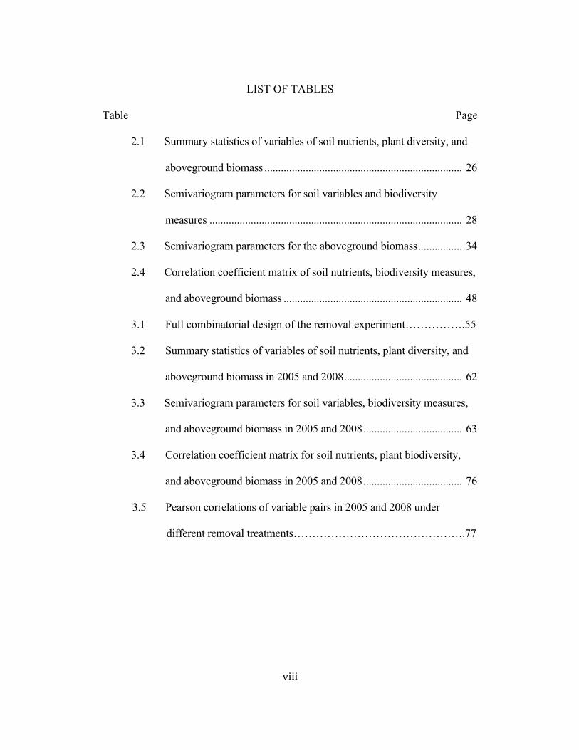
LIST OF TABLES
Table Page
2.1 Summary statistics of variables of soil nutrients, plant diversity, and
aboveground biomass ........................................................................ 26
2.2 Semivariogram parameters for soil variables and biodiversity
measures ............................................................................................ 28
2.3 Semivariogram parameters for the aboveground biomass ................ 34
2.4 Correlation coefficient matrix of soil nutrients, biodiversity measures,
and aboveground biomass ................................................................. 48
3.1 Full combinatorial design of the removal experiment…………….55
3.2 Summary statistics of variables of soil nutrients, plant diversity, and
aboveground biomass in 2005 and 2008 ........................................... 62
3.3 Semivariogram parameters for soil variables, biodiversity measures,
and aboveground biomass in 2005 and 2008 .................................... 63
3.4 Correlation coefficient matrix for soil nutrients, plant biodiversity,
and aboveground biomass in 2005 and 2008 .................................... 76
3.5 Pearson correlations of variable pairs in 2005 and 2008 under
different removal treatments……………………………………….77
ix
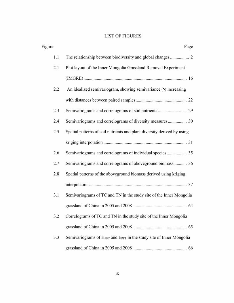
LIST OF FIGURES
Figure Page
1.1 The relationship between biodiversity and global changes ................. 2
2.1 Plot layout of the Inner Mongolia Grassland Removal Experiment
(IMGRE) ............................................................................................. 16
2.2 An idealized semivariogram, showing semivariance (γ) increasing
with distances between paired samples .............................................. 22
2.3 Semivariograms and correlograms of soil nutrients .......................... 29
2.4 Semivariograms and correlograms of diversity measures ................. 30
2.5 Spatial patterns of soil nutrients and plant diversity derived by using
kriging interpolation ........................................................................... 31
2.6 Semivariograms and correlograms of individual species .................. 35
2.7 Semivariograms and correlograms of aboveground biomass ............ 36
2.8 Spatial patterns of the aboveground biomass derived using kriging
interpolation ........................................................................................ 37
3.1 Semivariograms of TC and TN in the study site of the Inner Mongolia
grassland of China in 2005 and 2008 ................................................. 64
3.2 Correlograms of TC and TN in the study site of the Inner Mongolia
grassland of China in 2005 and 2008 ................................................. 65
3.3 Semivariograms of HPFT and EPFT in the study site of Inner Mongolia
grassland of China in 2005 and 2008 ................................................. 66
Figure Page
3.4 Correlograms of HPFT and EPFT in the study site of Inner Mongolia
grassland of China in 2005 and 2008 ................................................. 67
3.5 Semivariograms of PR, PB, PF, AB and AGB in the study site of
Inner Mongolia grassland of China in 2005 and 2008 ....................... 70
3.6 Correlograms of PR, PB, PF, AB and AGB in the study site of Inner
Mongolia grassland of China in 2005 and 2008 ................................ 71
CHAPTER 1: INTRODUCTION
IMPORTANCE OF SPATIAL HETEROGENEITY IN UNDERSTANDING
THE RELATIONSHIP BETWEEN BIODIVERSITY AND
ECOSYSTEM FUNCTIONING
1 Introduction
Since the beginning of the 20th century, intensive anthropogenic
disturbance has spawned the 6th major extinction event in the history of life,
leading to changes in species distribution across the world (Chapin et al. 2000). A
number of studies have demonstrated that changes in biodiversity (species
richness, evenness and composition) caused by global changes may significantly
alter the structure and functions of ecosystems, leading to degraded ecosystem
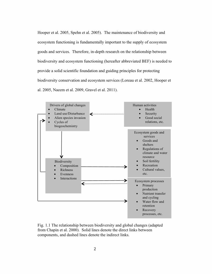
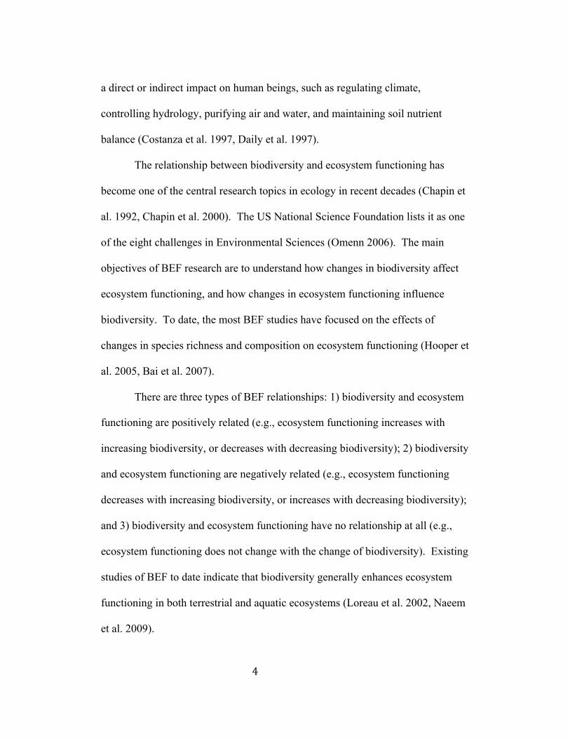
services that affect human social and economic activities (Fig. 1). The influences
of changes in biodiversity on ecosystem functioning have led to: 1) altered species
traits and thus ecosystem processes; 2) reduced utilization efficiency by plants for
water, nutrients and solar energy; 3) simplified food web structures and the
relationship of its associated components (nutrient structure); and 4) modified
disturbance regimes of various ecosystems (the frequency, intensity, and range of
disturbances) (Chapin et al. 1997, 2000).
Recent studies have shown that biodiversity affects structure, functioning,
and dynamics of ecosystems, and is one of the key factors in controlling stability,
productivity, nutrient cycling, and introduction of invasive species of ecosystems
(Naeem 1994, Tilman 1996, 1999, 2000, Chapin et al. 2000, Bai et al. 2004,
2
Hooper et al. 2005, Spehn et al. 2005). The maintenance of biodiversity and
ecosystem functioning is fundamentally important to the supply of ecosystem
goods and services. Therefore, in-depth research on the relationship between
biodiversity and ecosystem functioning (hereafter abbreviated BEF) is needed to
provide a solid scientific foundation and guiding principles for protecting
biodiversity conservation and ecosystem services (Loreau et al. 2002, Hooper et
al. 2005, Naeem et al. 2009, Gravel et al. 2011).
Fig. 1.1 The relationship between biodiversity and global changes (adapted from Chapin et al. 2000). Solid lines denote the direct links between components, and dashed lines denote the indirect links.
Drivers of global changes • Climate • Land use/Disturbance • Alien species invasion • Cycles of
biogeochemistry
Biodiversity • Composition • Richness • Evenness • Interactions
Ecosystem goods and services
• Goods and shelters
• Regulations of climate and water resource
• Soil fertility • Recreation • Cultural values,
etc.
Ecosystem processes • Primary
production • Nutrient transfer
and cycling • Water flow and
retention • Recovery
processes, etc.
Human activities • Health • Security • Good social
relations, etc.
3
2 The relationship between biodiversity and ecosystem functioning
Biodiversity was coined by E. O. Wilson in 1998 by combining the two
terms of “biological” and “diversity” (Wilson 1988). There are many definitions
for biodiversity, and the most commonly accepted definitions consist of three
levels of ecological organization: genetic, species and ecosystems. Biodiversity is
the ecological complex of biology and environment, and the sum of all associated
ecological processes, including millions of animals, plants, microorganisms,
genes, and complicated ecosystems formed by these organisms and their living
surroundings (Wilson 1988, 1993, Ma 1993, Gaston 1996, Purvis and Hector
2000, Mooney 2002). Biodiversity is a prerequisite of ecosystem functions and
services, which in turn provide the basis for the development and maintenance of
human society.
Definitions of ecosystem functioning have been defined from both broad
and narrow perspectives. Broadly, ecosystem functions include ecosystem
properties, ecosystem goods, and ecosystem services (Christensen et al. 1996).
Narrowly, the term refers only to ecosystem functions and properties, including
the size of ecosystem components (such as carbon or organic pools) and process
rates (such as ecosystem productivity, energy flow, material recycling and
information transfer rates, and ecosystem stability) (Hooper et al. 2005).
Ecosystem goods are those kinds of ecosystem properties that have direct market
value, including food, building materials, medicines, gene products, and
recreation. Ecosystem services refers to those properties of ecosystems that have
4
a direct or indirect impact on human beings, such as regulating climate,
controlling hydrology, purifying air and water, and maintaining soil nutrient
balance (Costanza et al. 1997, Daily et al. 1997).
The relationship between biodiversity and ecosystem functioning has
become one of the central research topics in ecology in recent decades (Chapin et
al. 1992, Chapin et al. 2000). The US National Science Foundation lists it as one
of the eight challenges in Environmental Sciences (Omenn 2006). The main
objectives of BEF research are to understand how changes in biodiversity affect
ecosystem functioning, and how changes in ecosystem functioning influence
biodiversity. To date, the most BEF studies have focused on the effects of
changes in species richness and composition on ecosystem functioning (Hooper et
al. 2005, Bai et al. 2007).
There are three types of BEF relationships: 1) biodiversity and ecosystem
functioning are positively related (e.g., ecosystem functioning increases with
increasing biodiversity, or decreases with decreasing biodiversity); 2) biodiversity
and ecosystem functioning are negatively related (e.g., ecosystem functioning
decreases with increasing biodiversity, or increases with decreasing biodiversity);
and 3) biodiversity and ecosystem functioning have no relationship at all (e.g.,
ecosystem functioning does not change with the change of biodiversity). Existing
studies of BEF to date indicate that biodiversity generally enhances ecosystem
functioning in both terrestrial and aquatic ecosystems (Loreau et al. 2002, Naeem
et al. 2009).
5
Most BEF studies have been field manipulative experiments in which
primary productivity is the focal variable for ecosystem functioning. Primary
productivity is a collective variable representing multiple ecosystem processes
(e.g., nutrient transfer and cycling, water flow, etc.) and has been one of the most
commonly used indicators of ecosystem function in many ecological studies for
decades (Whittaker and Levin 1975). Results from numerous BEF experiments to
date show that ecosystem productivity is positively related to biodiversity
(Hooper et al. 2005). Two primary mechanisms have been offered to explain the
positive relationship: first is niche complementarity effect, and second is selection
effect or sampling effect. Niche complementarity effect occurs when differences
in species resource requirements allow diverse communities to use available
resources more completely and efficiently and convert these resources into greater
biomass or other functions (Tilman et al. 1997, Loreau 2000, Spehn et al. 2005).
Selection effect or sampling effect refers to the phenomenon that increasing
biodiversity increases the possibility of species that are competitively superior and
functionally important being included in the community (Aarssen 1997, Huston
1997, Tilman 1997, 2001, Loreau 2000, Fox 2005, Spehn et al. 2005). However,
the two effects are not mutually exclusive, and both effects can operate
simultaneously to affect productivity.
The relationship between biodiversity and stability has been a central issue
in the BEF context. Because of the ambiguity in the definitions of biodiversity
and stability, and the complexity in the relationship between them, the diversity-
6
stability relationship has long been debated (Wu and Loucks 1995, Tilman 1999).
However, several studies suggest that the level of biodiversity plays a key part in
keeping the stability of ecosystem. David Tilman and his colleagues began a
long-term study to investigate the relationship between biodiversity and stability
in plant communities at Cedar Creek History Area, Minnesota, in 1982. They
found that diversity within an ecosystem tends to be correlated positively with the
stability of plant community (David and Downing 1994, Tilman 1996, Tilman et
al. 1996, Tilman et al. 2006). In a grassland of Temple, Texas, Isbell et al. (2009)
found that productivity was less variable among years in plots planted with more
species. The higher the level of biodiversity for an ecosystem is, the more the
number of genes and species there are, thus, the ecosystem can adapt itself better
to external stress. On the other side, stability is considered most meaningfully
with reference to disturbance or other external events. Disturbance has effects on
local diversity. A habitat with a high level of disturbance is extremely unstable
and can be tolerated usually only by few specially adapted species (Grime 1973).
A habitat with a low level of disturbance is highly stable, but often supports little
species richness because competitive exclusion has time to run its course.
Accordingly, empirical studies showed that the highest species richness often
occurs at intermediate disturbance intensity. Continued research in this area is
needed to explore the underlying mechanism behind the relationship between
biodiversity and ecosystem stability (Ives and Carpenter 2007).
7
3 Effects of spatial heterogeneity on the BEF relationships
Numerous studies have been carried out to explore the relationship
between biodiversity and ecosystem functioning (BEF) in natural ecosystems
(Lechmere-Oertel et al. 2005, Bai et al. 2007, Cheng et al. 2007, Grace et al.
2007). For example, Bai et al. (2007) reported that a positive linear, rather than
hump-shaped, form was ubiquitous across all the organizational levels of
association type, vegetation type and biome, and spatial scales of local, landscape
and regional in Inner Mongolia region of the Eurasian Steppe. A number of
mechanisms have been proposed to explain observed BEF relationships, and one
of them is spatial heterogeneity (Chesson 2000, Bailey et al. 2007). Spatial
heterogeneity, referring to unevenness and complexity of spatial distribution for
an ecological attribute (Kolasa and Pickett 1991), is considered as a ubiquitous
characterization of ecosystem processes (Pickett and Cadenasso 1995, Hutchings
2000, Hutchings et al. 2000, Wu et al. 2000, Turner and Cardille 2007). Spatial
heterogeneity is one of the major drivers behind species coexistence and
biodiversity at different scales (Wu and Loucks 1995).
Previous studies on BEF relationships have centered primarily on the
effects of species richness on ecosystem functioning at fine-scale and relatively
homogeneous communities (Tilman et al. 1996, 1997, Hooper et al 1999), with
little attention to the possible effects of spatial heterogeneity (Guo et al. 2006,
Duffy 2009). However, spatial heterogeneity may have important influences on
the BEF relationships especially on broad scales (Cardinale et al. 2000,
8
Deutschman 2001, Pachepsky et al. 2007, Tylianakis et al. 2008, Duffy 2009). A
growing body of BEF literature has documented that the shape and pattern of the
BEF relationships can depend critically on spatial heterogeneity in environment
(Fridley 2002, Cardinale et al. 2004, Wardle and Zackrisson 2005). For example,
resource heterogeneous distribution often strengthens the relationship between
plant biodiversity and productivity (Fridley 2002, Zhang and Zhang 2006).
Moreover, spatial heterogeneity represented as particular habitat types composing
the landscape could change the direction and magnitude of the slope relating
biodiversity and ecosystem functioning (Cardinale et al. 2000).
Spatial heterogeneity can have a variety of consequences on key variables
of biodiversity and ecosystem functioning. Spatial heterogeneity of
environmental conditions can increase the importance of species richness for an
ecosystem process (Griffin et al. 2009) and promote ecosystem functioning which
could be indicated by productivity (Wacker et al. 2008). A first step toward
understanding the effects of spatial heterogeneity on the BEF relationships is to
quantify spatial heterogeneity characteristics of key variables of biodiversity and
ecosystem functioning, and identify the spatial relationships among these
variables. Geostatistics has been a revolutionary tool to examine spatial
heterogeneity characteristics of variables of ecological processes in that the
parameters derived from the semivariogram model offer an index to quantify the
magnitude and scale of spatial heterogeneity for a variable studied (Curran 1988,
Meisel and Turner 1998).
9
In this thesis, I propose to examine how a selected set of variables
representing plant biodiversity and ecosystem functioning are spatially structured
and related to each other in a natural grassland in Inner Mongolia, China. This
study will take advantage of the data produced by the largest grassland BEF field
experiment – the Inner Mongolia Grassland Removal Experiment (IMGRE)
funded jointly by US NSF and Chinese NSF. The experiment was initiated in
2005 for background information investigation when the study site was in a
natural condition, and in the following years through 2006 to 2009, removal
treatments of plant functional types were conducted each year. Specifically, my
research will focus on the following two overarching research questions:
1. What are the spatial patterns of soil nutrients, plant biodiversity, and
aboveground biomass in a natural grassland community of Inner
Mongolia, China? How are they related spatially?
2. How do removal treatments affect the spatial patterns of soil nutrients,
plant biodiversity, and aboveground biomass? Is there any change for their
spatial correlations after removal treatments?
We predicted that soil nutrients, plant biodiversity, and aboveground
biomass in the natural grassland community would present different spatial
patterns, and they would be spatially correlated to each other closely. Removal
treatments will have a significant effect on spatial structures and spatial
correlations of variables, compared to those prior to the removal treatments.

10
These two research questions will be addressed through a series of spatial
analyses using traditional and spatial statistics. The field data for this study will
include the data from the IMGRE project as well as other studies in the Inner
Mongolia grassland region. The findings of our research are expected to provide
new insight into the spatial ecology of grasslands, and to help improve our
understanding of the BEF relationships and grassland management in the Inner
Mongolia grassland.
11
CHAPTER 2
SPATIAL PATTERNS OF SOIL NUTRIENTS, PLANT DIVERSITY, AND
ABOVEGROUND BIOMASS AND THEIR RELATIONSHIPS IN A
NATURAL GRASSLAND COMMUNITY IN INNER MONGOLIA, CHINA
1 Introduction
Spatial heterogeneity affects biodiversity as well as population and
ecosystem processes across a range of scales (Kolasa and Pickett 1991, Wu and
Loucks 1995). While understanding the dynamics and consequence of spatial
heterogeneity has been recognized as a central goal of landscape ecology (Turner
et al. 2001, Wu and Hobbs 2007), a “spatial” perspective has now become
pervasive in population, community, and ecosystem ecology and beyond because
heterogeneity is ubiquitous across systems and scales (Wu and Loucks 1995).
Ecosystem functioning in arid and semi-arid ecosystems is strongly
controlled by the spatial heterogeneity of soil water and nutrients (Wu and Levin
1994, Schlesinger et al. 1996, Reynolds et al. 1997, Olofsson et al. 2008).
Theoretical studies suggest that spatial heterogeneity in soil resources can
modulate the strength of BEF relationships (Tilman 1982, 1985). Spatial
heterogeneity can promote coexistence among species through resource or niche
partitioning (Tilman 1982, 1985). This notion is consistent with niche theory that
more species can coexist in a local area if they have complementary ways of
acquiring resources (Tilman and Kareiva 1997, Hutchings et al. 2003).
12
Consequently, higher species diversity will increase the rates of ecological
processes (McNaughton 1993).
While the relationship between biodiversity and ecosystem functioning
(BEF) has received considerable attention in the past few decades (Loreau et al.
2002, Hooper et al. 2005, Bai et al. 2007, Naeem et al. 2009), the effects of spatial
heterogeneity on the BEF relationships are still poorly understood. However,
numerous empirical studies suggest that spatial heterogeneity may significantly
influence how biodiversity and ecosystem functioning interact in different
landscapes. For example, Bai et al. (2007) found that, in the Eurasian steppe
region, plant species diversity and grassland net primary productivity both
increase along a regional environmental gradient with increasing precipitation,
and that the relationship between plant diversity and productivity may vary on
fine spatial scales. The BIODEPTH (Biodiversity and Ecological Processes in
Terrestrial Herbaceous Ecosystems) project carried out a series of BEF
experiments in seven European countries, and found that soil heterogeneity
between sites had significant effects on the experimental results (Hector et al.
1999, Hector and Hooper 2002, Hector et al. 2007). One of the major findings
from these experiments was that heterogeneity in soil properties across sites had
strong effects on the magnitude and variability of the measured effects, such as
Aboveground Net Primary Production (ANPP).
Within-site or within-community heterogeneity in environmental
resources may also significantly affect biodiversity and ecosystem functioning.
13
Studies have shown that differences in fine-scale topography and soil resources
may have significant effects on plant growth and species diversity (Schlesinger et
al. 1996, Reynolds et al. 1997, Olofsson et al. 2008). Zhou et al. (2008) found
that plant diversity was positively correlated with spatial heterogeneity of soil
nutrients in a semiarid grassland of Inner Mongolia in China. Factors affecting
broad-scale patterns of biodiversity and ecosystem processes may be quite
different from those on fine scales (Wu and Loucks 1995, Davies et al. 2005).
Although fine-scale environmental heterogeneity is likely to influence
biodiversity, ecosystem functioning, and their relationship, most BEF experiments
have assumed the environment within a biological community is spatially
homogeneous. This may potentially be a form of ‘hidden treatments’ (sensu
Huston 1997).
To help improve our understanding of the effects of fine-scale spatial
heterogeneity on the BEF relationships, a plausible first step is to quantify the
spatial patterns of variables representing biodiversity and ecosystem functioning,
and then examine the relationships between these two groups of variables in a
particular ecosystem. To do this, geostatistical techniques (Matheron 1963, David
1977) provide an effective approach. In recent decades, these methods have been
widely used to study spatial patterns of environmental factors and ecological
properties (Rossi et al. 1992, Fortin and Dale 2005). For example, semivariogram
modeling is suitable to quantify spatial structures of physical and biological
variables and detect the characteristics scales of spatial heterogeneity (Turner et
14
al. 1991, Robertson and Gross 1994, Burrough 1995, Kareiva and Wennergren
1995, Meisel and Turner 1998). Semivariograms can also be used in developing
sampling schemes that avoid the problems of spatial autocorrelation or pseudo-
replication (Legendre and Fortin 1989, Turner et al. 1991, Meisel and Turner
1998).
The main goal of this study was, therefore, to understand the spatial
patterns of abiotic and biotic variables relevant to biodiversity and ecosystem
functioning as well as their relationships, based on an existing BEF field
experiment in the Inner Mongolia grassland, China. We applied geostatistical
methods to examine the spatial patterns of soil nutrients, plant diversity, and
aboveground biomass at three organizational levels - the individual species, plant
functional types (PFTs), and the whole plant community. Two research questions
were addressed: 1) What are the spatial patterns of soil nutrients, plant
biodiversity and aboveground biomass? and 2) How are these variables related to
each other spatially and across the different levels of organization?
2 Materials and methods 2.1 Study site and experimental design
This study was based on the ongoing field manipulative experiment on the
biodiversity-ecosystem functioning relationship in the Inner Mongolia grassland
in northern China - the Inner Mongolia Removal Experiment (IMGRE). The
study site is located in a L. chinensis-dominant community in the Xilin River
15
Basin of Inner Mongolia Autonomous Region of China (116°42′E, 43°38′N). The
long-term annual mean air temperature is 0.6 ºC. The coldest month (January) is
characterized by the mean temperature of -21.6 ºC, and the mean temperature of
the warmest month (July) is 19.0 ºC. Topographic relief exhibits little variation,
with elevation ranging from 1,250-1,260 m at the experimental site. Mean annual
precipitation is 346.1 mm with 60-80% occurring during the growing season from
May to August. Main soil type is chestnut soils with similar physiochemical
properties throughout the site. Vegetation of the region consists of the dominant
species Leymus chinensis (LC) and Stipa grandis (SG), and five non-dominant
species Achnatherum sibiricum (AS), Cleistogenes squarrosa (CS), Koeleria
cristata (KC), Agropyron cristatum (AC) and Allium tenuissimum (AT), etc.
There are 86 species in the plant community, which fall into five plant functional
types based on their life forms: perennial rhizome (PR), perennial bunchgrasses
(PB), perennial forbs (PF), annuals and biennials (AB), and shrubs and semi-
shrubs (SS) (Bai et al. 2004).
16
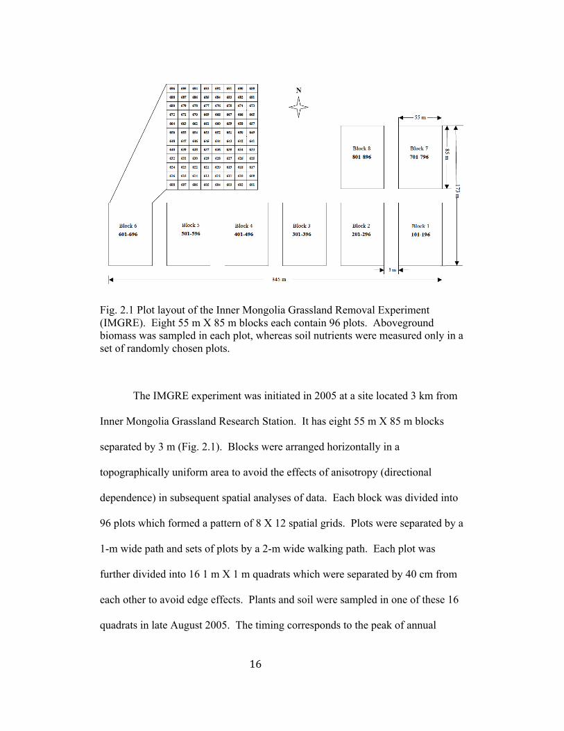
Fig. 2.1 Plot layout of the Inner Mongolia Grassland Removal Experiment (IMGRE). Eight 55 m X 85 m blocks each contain 96 plots. Aboveground biomass was sampled in each plot, whereas soil nutrients were measured only in a set of randomly chosen plots.
The IMGRE experiment was initiated in 2005 at a site located 3 km from
Inner Mongolia Grassland Research Station. It has eight 55 m X 85 m blocks
separated by 3 m (Fig. 2.1). Blocks were arranged horizontally in a
topographically uniform area to avoid the effects of anisotropy (directional
dependence) in subsequent spatial analyses of data. Each block was divided into
96 plots which formed a pattern of 8 X 12 spatial grids. Plots were separated by a
1-m wide path and sets of plots by a 2-m wide walking path. Each plot was
further divided into 16 1 m X 1 m quadrats which were separated by 40 cm from
each other to avoid edge effects. Plants and soil were sampled in one of these 16
quadrats in late August 2005. The timing corresponds to the peak of annual
17
aboveground net primary production (ANPP) in temperate grasslands (Sala and
Austin 2000, Bai et al. 2004). Specific measurements included species richness
(the number of species in a specified area), the aboveground biomass of
individual species, total carbon (TC), total nitrogen (TN), and total phosphorous
(TP).
2.2 Vegetation sampling and measurements
We clipped the stem of live plant at the ground level of live plants in one
of the 16 quadrates in each plot (768 plots in total) and sorted material by species.
All samples were oven-dried to a constant mass at 65 ℃ for a minimum of 48 h.
Aboveground biomass (g) was measured by plant species and then grouped into
categories of plant functional types.
The species diversity of a plant community can be measured in three ways.
First, species richness (S) is simply the number of species in a plant community
(or a sampling area). Second, information theoretic indices are often used to
capture the diversity of species in terms of both their richness (the number of
species) and relative abundances (evenness). The most frequently used species or
plant functional type diversity index is the Shannon-Weaver index (H):
H = ! (Pi lnPi )i=1
s
! (1)
where S is the total number of species or plant functional types in the plot, and Pi
is the biomass proportion of the ith species or plant functional type. For a given
number of species in a community, the more even the relative abundance among

18
the species is, the higher the value of H will be. In our study, we used the relative
aboveground biomass (the percentage of a species’ aboveground biomass relative
to the total aboveground biomass of all species) to represent the relative
abundance of a species in the community. There is no upper bound to the values
of this index.
Third, species evenness (E) is a measure of how similar the abundance of
different species is in a community. The Shannon evenness index is computed as:
E = HHmax
= HlnS
(2)
where H is the Shannon-Weaver index calculated as shown above. When the
proportions of all species are similar, evenness is close to one. When the
abundances of different species are quite dissimilar (e.g., some rare and some
common), the value of evenness will be much larger than one.
2.3 Soil sampling and measurements
Soil samples were collected in evenly distributed plots across the same
research site. Three soil samples, which form a triangle around each plot center,
were collected using a 3-cm diameter soil auger to a depth of 20 cm immediately
after plant harvesting and removal of surface litter. Samples from the same plot
were mixed as one composite sample and air-dried in a ventilation room, cleared
of roots and organic debris, and passed through 2-mm sieves for further chemical
analysis. Total carbon (TC) was analyzed following a modified Meius method,
19
total nitrogen (TN) - by the Kjeladahl digestion procedure, and total phosphorus
(TP) - by the digestion of soil samples with perchloric acid.
All the sampling and measurements for vegetation and soil properties were
done by the IMGRE research team, including a large number of faculty and
graduate students from Institute of Botany of the Chinese Academy of Sciences
and School of Life Sciences, Arizona State University.
2.4 Data analysis
Several variables were selected in our analysis based on their relevance to
the BEF relationships. These include: spatial variability of soil nutrients (TC, TN,
and TP) in sampled plots, plant biodiversity measures (number of species (NSP),
species diversity index (HSP), species evenness index (ESP), plant functional type
diversity index (HPFT), and plant functional type evenness index (EPFT)), and
aboveground biomass at the organizational levels of individual species, plant
functional type and the whole community of each plot.
Spatial autocorrelation analysis provides a quantitatively unbiased
estimate of the spatial correlation between sampled values as a function of their
lag distances. A common geostatistical method, semivariance analysis, can be
employed to quantify spatial autocorrelation and spatial dependence of ecological
patterns (Rossi et al. 1992). The semivariance is calculated as:
! (h) = 12N(h)
[z(xi )! z(xi + h)]2
i=1
N (h)
! (3)
20
where N(h) is the number of pairs of data at each distance interval (lag) h, and
z(xi) and z(xi+h) are measurements at sampling points separated by a lag of h.
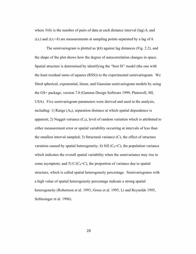
The semivariogram is plotted as γ(h) against lag distances (Fig. 2.2), and
the shape of the plot shows how the degree of autocorrelation changes in space.
Spatial structure is determined by identifying the “best fit” model (the one with
the least residual sums of squares (RSS)) to the experimental semivariogram. We
fitted spherical, exponential, linear, and Gaussian semivariogram models by using
the GS+ package, version 7.0 (Gamma Design Software 1999, Plainwell, MI,
USA). Five semivariogram parameters were derived and used in the analysis,
including: 1) Range (A0), separation distance at which spatial dependence is
apparent; 2) Nugget variance (C0), level of random variation which is attributed to
either measurement error or spatial variability occurring at intervals of less than
the smallest interval sampled; 3) Structural variance (C), the effect of structure
variation caused by spatial heterogeneity; 4) Sill (C0+C), the population variance
which indicates the overall spatial variability when the semivariance may rise to
some asymptote; and 5) C/(C0+C), the proportion of variance due to spatial
structure, which is called spatial heterogeneity percentage. Semivariograms with
a high value of spatial heterogeneity percentage indicate a strong spatial
heterogeneity (Robertson et al. 1993, Gross et al. 1995, Li and Reynolds 1995,
Schlesinger et al. 1996).

21
Moran’s I, a global measure of spatial autocorrelation was also used to
identify the degree of spatial dependence on variables over distances in our study
(Moran 1948). Moran’ I is calculated with the following formula:
I =n ! ij(xi ! x
j=1
n
"i=1
n
" )(x j ! x)
( ! ij ) (xi ! x)2
i=1
n
"j=1
n
"i=1
n
"(4)
where xi and x j refer to the measured sample values at i and j, respectively, x j is
the average value of x, ! ij is the weighted matrix value, and n is the number of
pairs of data. Values of I range between -1 and 1 with positive values
corresponding to positive autocorrelation, zero indicating randomness, and
negative values representing negative autocorrelation. Calculating this index for a
variety of lag distances yields Moran’s I correlograms. The correlograms were
generated by using the GS+ package.
Semivariance and Moran’s I are complementary for evaluating the spatial
structure of data. In our study, the minimum lag distance was 7 m, which
corresponds to the minimal distance between sampled plots, while the maximum
lag distance was extended to 186 m (approximately equals 50% of the distance
between the largest lag pair) (Rossi et al. 1992). We performed block kriging
mapping with calculated semivariograms for the aforementioned variables, except
the rare plant functional types AB and SS because of too few samples for AB and
no samples for SS.
22
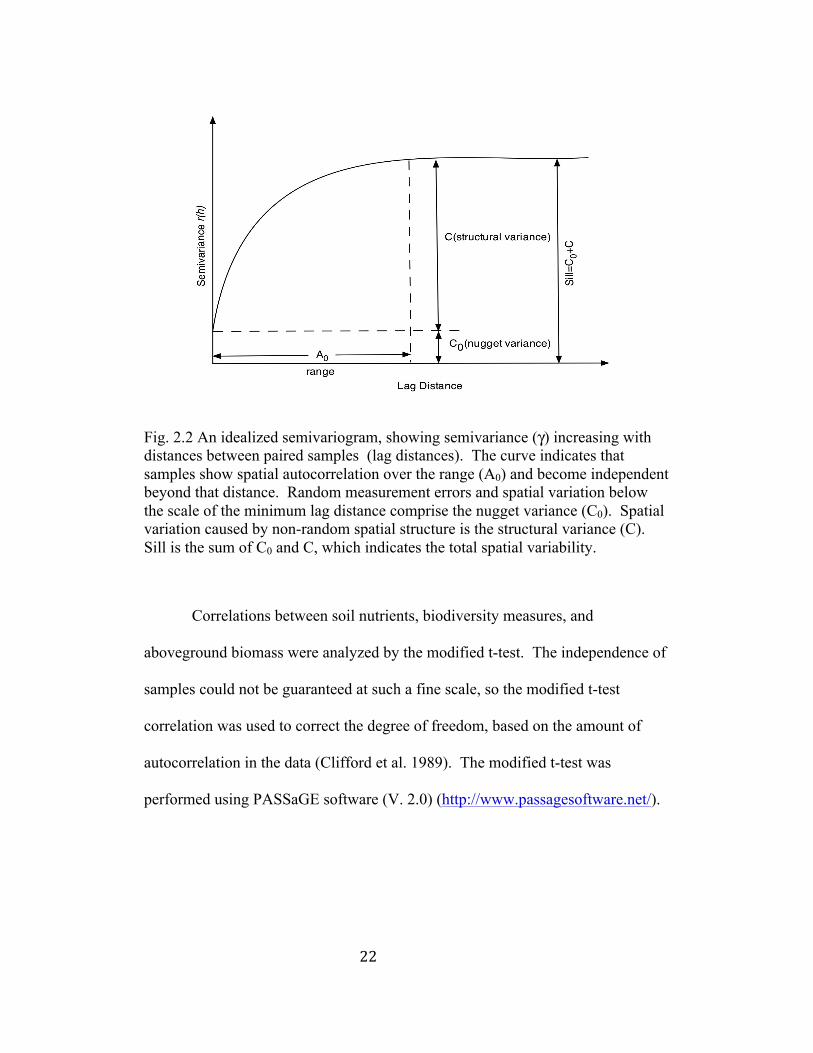
Fig. 2.2 An idealized semivariogram, showing semivariance (γ) increasing with distances between paired samples (lag distances). The curve indicates that samples show spatial autocorrelation over the range (A0) and become independent beyond that distance. Random measurement errors and spatial variation below the scale of the minimum lag distance comprise the nugget variance (C0). Spatial variation caused by non-random spatial structure is the structural variance (C). Sill is the sum of C0 and C, which indicates the total spatial variability.
Correlations between soil nutrients, biodiversity measures, and
aboveground biomass were analyzed by the modified t-test. The independence of
samples could not be guaranteed at such a fine scale, so the modified t-test
correlation was used to correct the degree of freedom, based on the amount of
autocorrelation in the data (Clifford et al. 1989). The modified t-test was
performed using PASSaGE software (V. 2.0) (http://www.passagesoftware.net/).
23
3 Results
3.1 Summary statistics of variables of soil nutrients, plant biodiversity, and
aboveground biomass
Averaged over the sampled plots, mean values of TC, TP, and TN were
47.98 ± 0.07 g⋅kg-1, 4.88 ± 0.07 g⋅kg-1, and 7.23 ± 0.10 g⋅kg-1, respectively. Mean
species richness was 8 ± 0.05 m-2, species diversity index (Hsp) at the plot level
was 1.46 ± 0.21, and the plant functional type diversity index (HPFT) was 0.76 ±
0.21 (Table 2.1). The smallest value of aboveground biomass of seven individual
species in the study was observed in A. tenuissimum (1.45 ± 1.28 g⋅m-2), while L.
chinensis and S. grandis contributed the most to the total aboveground biomass.
When grouped by plant functional type, perennial bunchgrasses were the main
contributor to the total aboveground biomass (Table 2.1). Coefficients of
variation (CV) - which is the ratio of standard deviation to the mean - ranged from
16% for NSP to 130% for the annuals and biennuals functional type (Table 2.1).
The coefficients of skewness and kurtosis could be used to describe the shape of
the sample distribution. The majority of variables, except TC, TP, ESP, HPFT, EPFT
and perennial bunchgrasses, showed positively skewed distributions. Most
variables had distributions with positive kurtosis, indicating a “peaked”
distribution, while TC, HPFT, EPFT, and S. grandis were characterized by relatively
smooth distributions owing to the negative kurtosis (Table 2.1).
24
3.2 Spatial patterns of soil nutrients, plant biodiversity, and aboveground
biomass
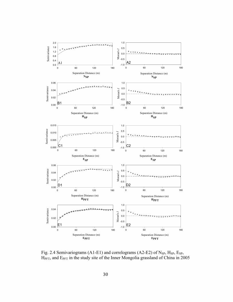
3.2.1 Soil nutrients
The “best-fit” model to the semivariograms of soil nutrients in our study
was spherical model, indicating the presence of spatial autocorrelation within a
certain distance defined by the range (Table 2.2, Fig. 2.3 A1-C1). Spatial
autocorrelation ranges varied from 69.30 m for TP to 102.30 m for TN. The
values of spatial heterogeneity percentage were high, ranging from 73% (TN) to
99% (TP), which suggests high spatial structure. The high values (above 50%) of
spatial heterogeneity percentage also suggested that spatially structured variance
accounted for a larger proportion of the total sample variance in soil nutrients
(Table 2.2). Compared to other soil nutrients, TP had higher r2 and lower nugget
values in the semivariogram model (Table 2.2). All soil nutrient variables were
positively autocorrelated within 60 m, and then showed negative autocorrelation
at greater lag distances (Fig. 2.3 A2-C2). Kriging maps illustrated that spatial
patterns of soil nutrients were considerably correlated with each other (Fig. 2.5 A-
C). The island of low values of the three soil variables was apparent in block 1 of
the study site. Higher values of soil nutrients were found in blocks 2 and 3 (Fig.
2.5 A-C).
25
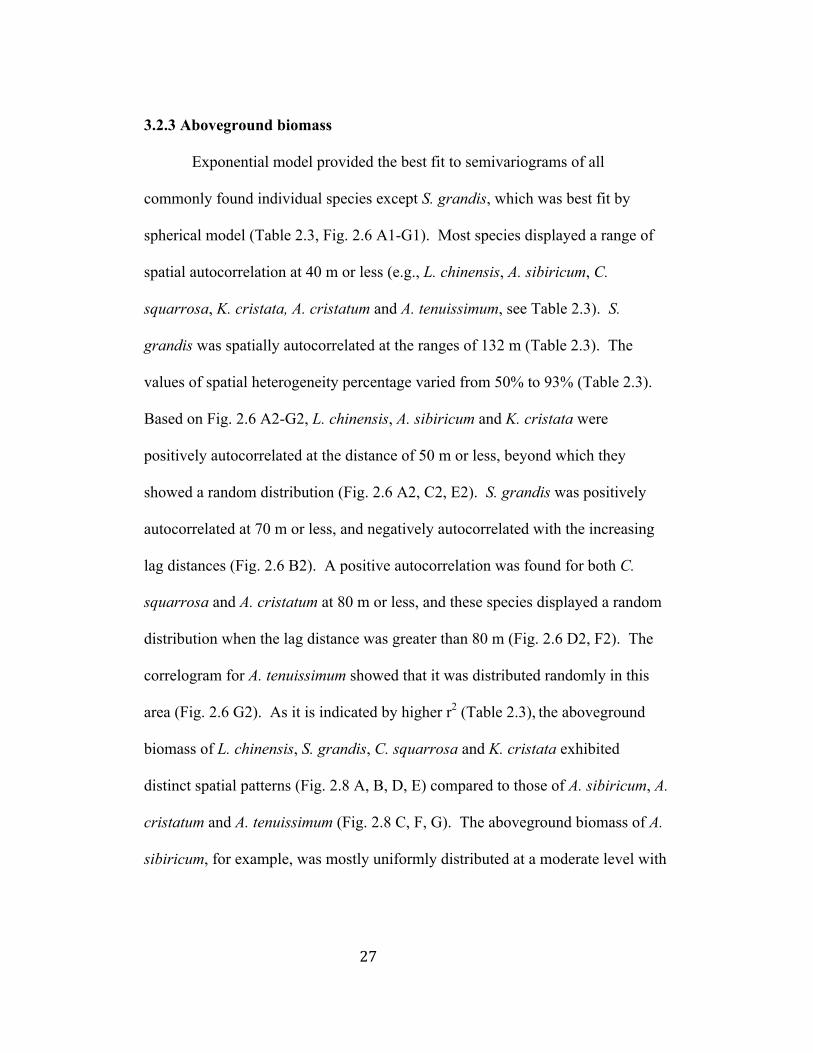
3.2.2 Plant biodiversity
The “best-fit” model for most plant biodiversity measures was exponential
model (Table 2.2, Fig. 2.4 A1-E1). The only exception was HSP where spherical
model provided the best fit (Table 2.2). The ranges of NSP, HSP, ESP, HPFT, and
EPFT were 39.90 m, 118.50 m, 13.20 m, 26.60 m, and 28.20 m, respectively (Table
2.2). All semivariograms of NSP, HSP, ESP, HPFT, and EPFT exhibited distinctive
patterns (Fig. 2.4 A1-E1) as indicated by high r2, low RSS, relatively low nugget
values (Table 2.2). From Fig. 2.4, NSP, HSP, and ESP exhibited positive
autocorrelations within 80 m, and then showed negative autocorrelations and no
correlations with increasing lag distances (Fig. 2.4 A2-C2). HPFT and EPFT were
positively autocorrelated within 75 m, and then showed negative autocorrelations
and no correlations at greater lag distances (Fig. 2.4 D2-E2). Kriging maps
showed higher values of NSP and HSP were concurrent in blocks 1 and 2 (Fig. 2.5
D, E). Moreover, HPFT and EPFT showed appropriately identical spatial patterns
(Fig. 2.5 G and H).
26
27
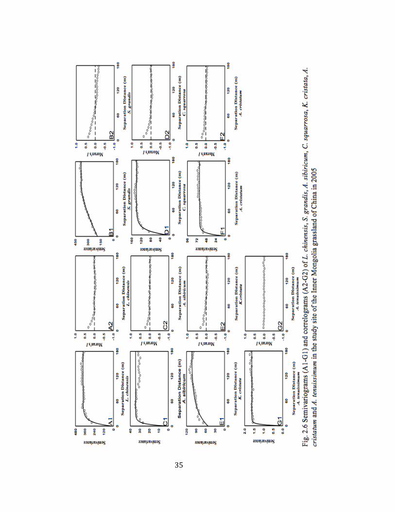
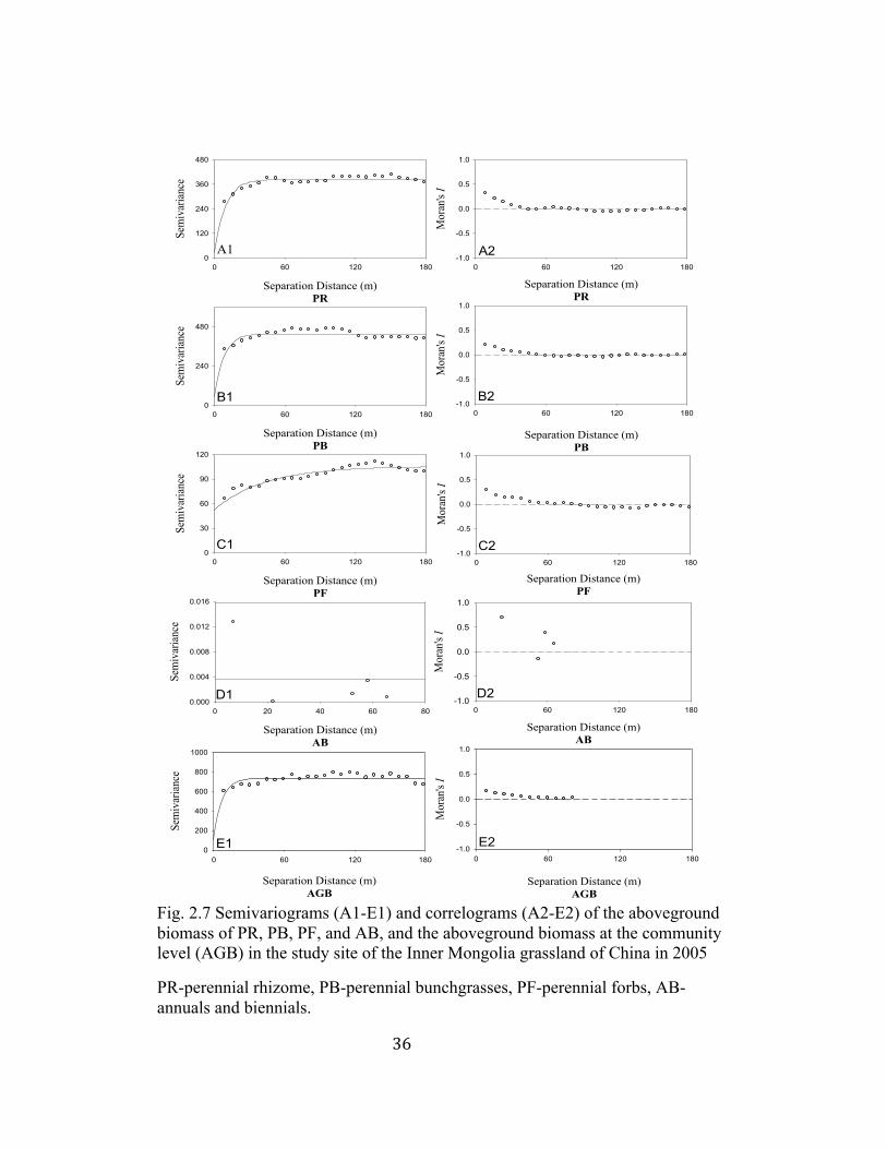
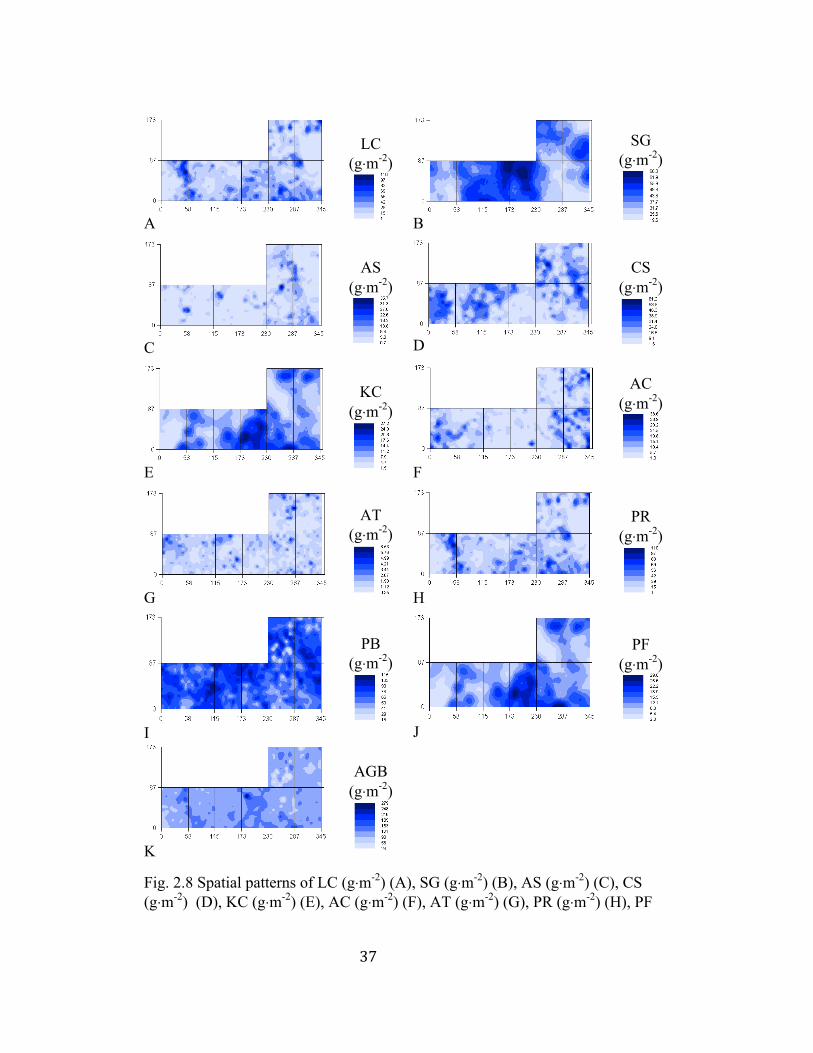
3.2.3 Aboveground biomass
Exponential model provided the best fit to semivariograms of all
commonly found individual species except S. grandis, which was best fit by
spherical model (Table 2.3, Fig. 2.6 A1-G1). Most species displayed a range of
spatial autocorrelation at 40 m or less (e.g., L. chinensis, A. sibiricum, C.
squarrosa, K. cristata, A. cristatum and A. tenuissimum, see Table 2.3). S.
grandis was spatially autocorrelated at the ranges of 132 m (Table 2.3). The
values of spatial heterogeneity percentage varied from 50% to 93% (Table 2.3).
Based on Fig. 2.6 A2-G2, L. chinensis, A. sibiricum and K. cristata were
positively autocorrelated at the distance of 50 m or less, beyond which they
showed a random distribution (Fig. 2.6 A2, C2, E2). S. grandis was positively
autocorrelated at 70 m or less, and negatively autocorrelated with the increasing
lag distances (Fig. 2.6 B2). A positive autocorrelation was found for both C.
squarrosa and A. cristatum at 80 m or less, and these species displayed a random
distribution when the lag distance was greater than 80 m (Fig. 2.6 D2, F2). The
correlogram for A. tenuissimum showed that it was distributed randomly in this
area (Fig. 2.6 G2). As it is indicated by higher r2 (Table 2.3), the aboveground
biomass of L. chinensis, S. grandis, C. squarrosa and K. cristata exhibited
distinct spatial patterns (Fig. 2.8 A, B, D, E) compared to those of A. sibiricum, A.
cristatum and A. tenuissimum (Fig. 2.8 C, F, G). The aboveground biomass of A.
sibiricum, for example, was mostly uniformly distributed at a moderate level with
28
just a few patches with higher values (Fig. 2.8 C). The aboveground biomass of S.
grandis was higher in the center of the study site (Fig. 2.8 B).
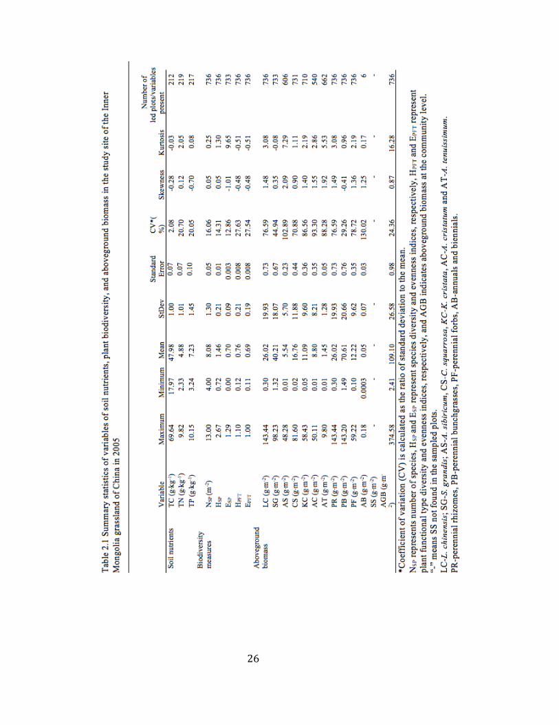
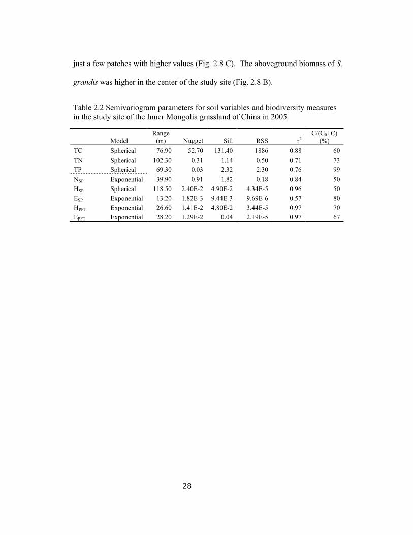
Table 2.2 Semivariogram parameters for soil variables and biodiversity measures in the study site of the Inner Mongolia grassland of China in 2005
Model Range
(m) Nugget Sill RSS r2 C/(C0+C)
(%) TC Spherical 76.90 52.70 131.40 1886 0.88 60 TN Spherical 102.30 0.31 1.14 0.50 0.71 73 TP Spherical 69.30 0.03 2.32 2.30 0.76 99 NSP Exponential 39.90 0.91 1.82 0.18 0.84 50 HSP Spherical 118.50 2.40E-2 4.90E-2 4.34E-5 0.96 50 ESP Exponential 13.20 1.82E-3 9.44E-3 9.69E-6 0.57 80 HPFT Exponential 26.60 1.41E-2 4.80E-2 3.44E-5 0.97 70 EPFT Exponential 28.20 1.29E-2 0.04 2.19E-5 0.97 67

29
Separation Distance (m)TN
0 60 120 180
Mor
an's
I
-1.0
-0.5
0.0
0.5
1.0
Separation Distance (m)TC
0 60 120 180
Sem
ivar
ianc
e
0.0
0.4
0.8
1.2
1.6
Separation Distance (m)TC
0 60 120 180
Mor
an's
I
-1.0
-0.5
0.0
0.5
1.0
Separation Distance (m)TN
0 60 120 180
Sem
ivar
ianc
e
0.000
0.006
0.012
0.018
Separation Distance (m)TP
0 60 120 1800.00
0.01
0.02
0.03
Separation Distance (m)TP
0 60 120 180-1.0
-0.5
0.0
0.5
1.0
Sem
ivar
ianc
e
Mor
an's
I
A1 A2
B1 B2
C1 C2
Fig. 2.3 Semivariograms (A1-C1) and correlograms (A2-C2) of TC, TN, and TP in the study site of the Inner Mongolia grassland of China in 2005
30
0 60 120 180
Sem
ivar
ianc
e
0.0
0.4
0.8
1.2
1.6
2.0
Separation Distance (m)NSP
0 60 120 180
Mor
an's I
-1.0
-0.5
0.0
0.5
1.0
Separation Distance (m)HSP
0 60 120 180
Sem
ivar
ianc
e
0.00
0.02
0.04
0.06
Separation Distance (m)HSP
0 60 120 180
Mor
an's I
-1.0
-0.5
0.0
0.5
1.0
Separation Distance (m)ESP
0 60 120 180-1.0
-0.5
0.0
0.5
1.0
Separation Distance (m)NSP
0 60 120 180
Sem
ivar
ianc
e
0.000
0.005
0.010
0.015
Mor
an's I
Separation Distance (m)HPFT
0 60 120 180
Sem
ivar
ianc
e
0.00
0.02
0.04
0.06
0 60 120 180
Mor
an's I
-1.0
-0.5
0.0
0.5
1.0
Separation Distance (m)ESP
Separation Distance (m)HPFT
0 60 120 180
Sem
ivar
ianc
e
0.00
0.02
0.04
Separation Distance (m)EPFT
0 60 120 180-1.0
-0.5
0.0
0.5
1.0
Mor
an's I
Separation Distance (m)EPFT
A1 A2
B1 B2
C1 C2
D1 D2
E1 E2
Fig. 2.4 Semivariograms (A1-E1) and correlograms (A2-E2) of NSP, HSP, ESP, HPFT, and EPFT in the study site of the Inner Mongolia grassland of China in 2005
31
A
TC (g⋅kg-1)
B
TN (g⋅kg-
1)
C
TP (g⋅kg-1)
D
NSP
E
HSP
F
ESP
G
HPFT
H
EPFT
Fig. 2.5 Spatial patterns of TC (g⋅kg-1) (A), TN (g⋅kg-1) (B), TP (g⋅kg-1) (C), NSP (D), HSP (E), ESP (F), HPFT (G), and EHPT (H) derived by using kriging interpolation in the study site of the Inner Mongolia grassland of China in 2005
Exponential model was the best fit to the semivariograms for most
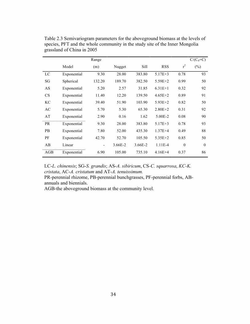
aboveground biomass of plant functional types (Table 2.3, Fig. 2.6). The annuals
and biennials functional type with only six samples was best fit by linear model
(Table 2.3, Fig. 2.6 D). Two dominant plant functional types of perennial
rhizome and perennial bunchgrasses displayed ranges of spatial autocorrelation at
9.30 m and 7.80 m, respectively, whereas perennial forbs had the range value of
32
42.70 m, and annuals and biennials had no range value because of few samples
found in the study site (Table 2.3). The values of spatial heterogeneity percentage
were above 50% for perennial rhizome, perennial bunchgrasses and perennial
forbs, indicating higher spatial structures in these plant functional types (Table
2.3). The aboveground biomass of perennial rhizome and perennial forbs
exhibited distinct patchiness (Fig. 2.7 H, J), supported by the high r2 (Table 2.3).
Correlograms showed that perennial rhizome and perennial bunchgrasses were
positively autocorrelated within 50 m, and then were randomly distributed with
the increasing lag distances (Fig. 2.7 A2, B2). The non-dominant plant functional
type of perennial forbs was positively autocorrelated within 80 m, and then
negatively autocorrelated between 80 m and 150 m (Fig. 2.7 C2). The perennial
bunchgrasses functional type was characterized by high biomass distributed
homogenously across the study site (Fig. 2.7 I).
Exponential model provided the best fit to semivariograms of the
aboveground biomass at the community level (AGB) (Table 2.3). The range of
AGB was 6.90 m, and the value of spatial heterogeneity percentage was 86% at
this level. No distinctive patchiness can be found at this level (Fig. 2.7 K), which
was also suggested by the low value of r2 (Table 2.3).
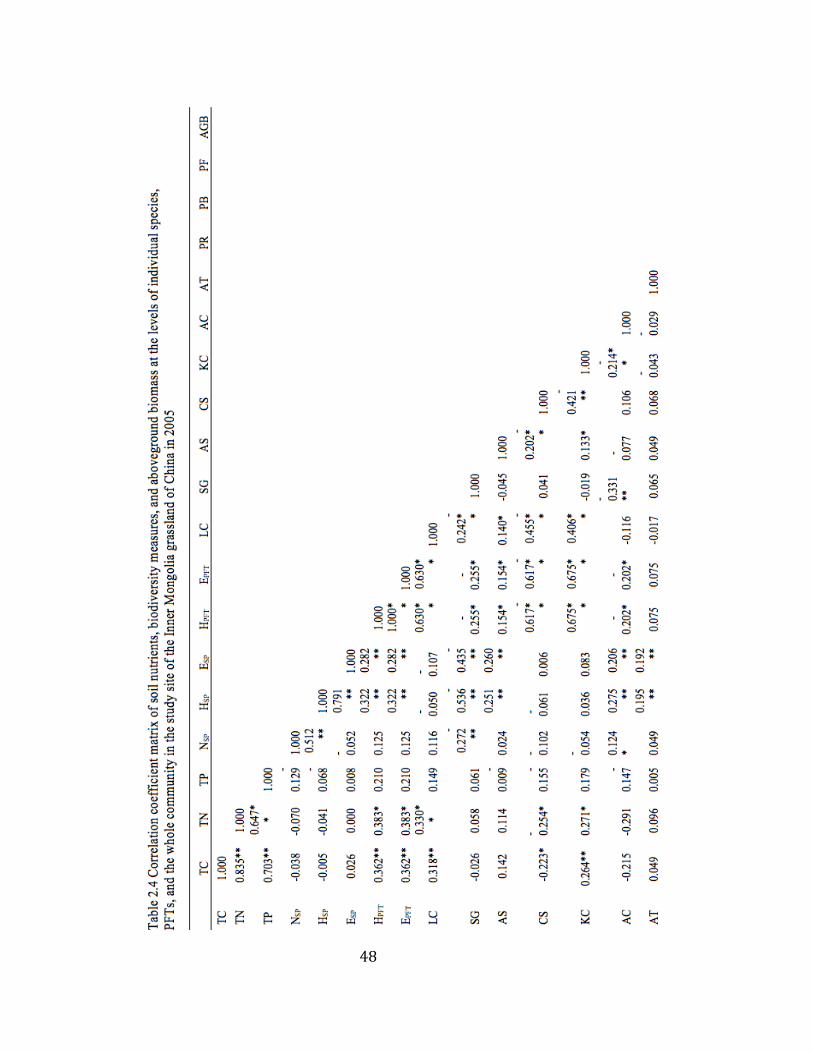
3.3 Correlations among soil nutrients, plant biodiversity, and aboveground
biomass
Correlation analysis was performed to explore the relationships among
soil nutrients, plant biodiversity measures and the aboveground biomass at the
33
levels of individual species, plant functional type and the whole community
(Table 2.4). Note that the correlation between the annuals and biennials
functional type and any other variable was not conducted because its sample size
was too small. Strongly positive correlations (0.647 < r < 0.835 and P < 0.01)
were found between TC and TN, between TC and TP, and between TN and TP.
In terms of plant biodiversity measures, significantly positive correlations (0.282
< r < 0.791 and P < 0.01) existed between NSP and HSP, between HSP and ESP,
HPFT, and EPFT, between ESP and HPFT and EPFT, and between HPFT and EPFT.
TC was significantly positively correlated (P < 0.01) to HPFT, EPFT, L.
chinensis, K. cristata, perennial rhizome and perennial forbs, and TN was
positively correlated (P < 0.01) to HPFT, EPFT, L. chinensis, perennial rhizome and
perennial forbs. There were no significant correlations between TP and variables
of plant biodiversity measures and aboveground biomass.
34
Table 2.3 Semivariogram parameters for the aboveground biomass at the levels of species, PFT and the whole community in the study site of the Inner Mongolia grassland of China in 2005
Model
Range
(m) Nugget Sill RSS r2
C/(C0+C)
(%)
LC Exponential 9.30 28.00 383.80 5.17E+3 0.78 93
SG Spherical 132.20 189.70 382.50 5.59E+2 0.99 50
AS Exponential 5.20 2.57 31.85 6.31E+1 0.32 92
CS Exponential 11.40 12.20 139.50 4.65E+2 0.89 91
KC Exponential 39.40 51.90 103.90 5.93E+2 0.82 50
AC Exponential 5.70 5.30 65.30 2.80E+2 0.31 92
AT Exponential 2.90 0.16 1.62 5.00E-2 0.08 90
PR Exponential 9.30 28.00 383.80 5.17E+3 0.78 93
PB Exponential 7.80 52.00 435.30 1.37E+4 0.49 88
PF Exponential 42.70 52.70 105.50 5.35E+2 0.85 50
AB Linear - 3.66E-2 3.66E-2 1.11E-4 0 0
AGB Exponential 6.90 105.00 735.10 4.16E+4 0.37 86
LC-L. chinensis; SG-S. grandis; AS-A. sibiricum, CS-C. squarrosa, KC-K. cristata, AC-A. cristatum and AT-A. tenuissimum. PR-perennial rhizome, PB-perennial bunchgrasses, PF-perennial forbs, AB-annuals and biennials. AGB-the aboveground biomass at the community level.
35
36
Separation Distance (m)PR
0 60 120 180
Sem
ivar
ianc
e
0
120
240
360
480
Separation Distance (m)PR
0 60 120 180
Mor
an's
I
-1.0
-0.5
0.0
0.5
1.0
Separation Distance (m)PB
0 60 120 180
Sem
ivar
ianc
e
0
240
480
Separation Distance (m)PB
0 60 120 180
Mor
an's
I
-1.0
-0.5
0.0
0.5
1.0
Separation Distance (m)PF
0 60 120 180
Sem
ivar
ianc
e
0
30
60
90
120
Separation Distance (m)PF
0 60 120 180
Mor
an's
I
-1.0
-0.5
0.0
0.5
1.0
Separation Distance (m)AB
0 20 40 60 80
Sem
ivar
ianc
e
0.000
0.004
0.008
0.012
0.016
Separation Distance (m)AB
0 60 120 180
Mor
an's
I
-1.0
-0.5
0.0
0.5
1.0
Separation Distance (m)AGB
0 60 120 180
Sem
ivar
ianc
e
0
200
400
600
800
1000
Separation Distance (m)AGB
0 60 120 180
Mor
an's
I
-1.0
-0.5
0.0
0.5
1.0
A1 A2
B1 B2
C1 C2
D1 D2
E1 E2
Fig. 2.7 Semivariograms (A1-E1) and correlograms (A2-E2) of the aboveground biomass of PR, PB, PF, and AB, and the aboveground biomass at the community level (AGB) in the study site of the Inner Mongolia grassland of China in 2005
PR-perennial rhizome, PB-perennial bunchgrasses, PF-perennial forbs, AB-annuals and biennials.
37
A
LC (g⋅m-2)
B
SG (g⋅m-2)
C
AS (g⋅m-2)
D
CS (g⋅m-2)
E
KC (g⋅m-2)
F
AC (g⋅m-2)
G
AT (g⋅m-2)
H
PR (g⋅m-2)
I
I
PB (g⋅m-2)
J
PF (g⋅m-2)
K
AGB (g⋅m-2)
Fig. 2.8 Spatial patterns of LC (g⋅m-2) (A), SG (g⋅m-2) (B), AS (g⋅m-2) (C), CS (g⋅m-2) (D), KC (g⋅m-2) (E), AC (g⋅m-2) (F), AT (g⋅m-2) (G), PR (g⋅m-2) (H), PF
38
(g⋅m-2) (I), PB (g⋅m-2) (J) and AGB (g⋅m-2) (K) derived using kriging interpolation in the study site of the Inner Mongolia grassland of China in 2005
LC-L. chinensis; SG-S. grandis; AS-A. sibiricum; CS-C. squarrosa; KC-K. cristata; AC-A. cristatum and AT-A. tenuissimum. PR-perennial rhizome, PB-perennial bunchgrasses, PF-perennial forbs, AB-annuals and biennials. AGB-the aboveground biomass at the community level.
For the aboveground biomass of individual species, the dominant species
L. chinensis was significantly positively correlated (P < 0.01) with plant
biodiversity measures of HPFT and EPFT, the other dominant species S. grandis was
significantly negatively correlated (P < 0.01) with NSP, ESP and HSP, whereas non-
dominant species including A. sibiricum, A. cristatum and A. tenuissimum were
significantly positively correlated (P < 0.01) with ESP and HSP. With respect to 21
species pairs constructed from the seven species, a significant positive correlation
(P < 0.01) was found only for one pair (the dominant species L. chinensis versus
the non-dominant species K. cristata), while a negative correlation (P < 0.01) was
found for six pairs (e.g., L. chinensis versus S. grandis, L. chinensis versus C.
squarrosa, L. chinensis versus K. cristata, S. grandis versus A. cristatum, A.
sibiricum versus C. squarrosa, and C. squarrosa versus K. cristata). The
dominant species, L. chinensis and S. grandis, were significantly negatively
correlated (P < 0.01) (Table 2.4).
For the aboveground biomass of plant functional types, the three plant
functional types of perennial rhizome, perennial bunchgrasses and perennial forbs
were significantly correlated (P < 0.01) with HPFT and EPFT, either positively or
39
negatively. A significantly positive correlation (P < 0.01) existed between the
perennial rhizome functional type and the perennial forbs functional type, and a
significantly negative correlation (P < 0.01) was found between the perennial
bunchgrasses functional type and the perennial forbs functional type. Two
dominant plant functional types, the perennial rhizome and the perennial
bunchgrasses, were significantly negatively correlated (P < 0.01) (Table 2.4).
The aboveground biomass at the community level (AGB) was
significantly positively correlated (P < 0.01) with the individual species of L.
chinensis, S. grandis, A. sibiricum, K. cristata and A. tenuissimum, and the plant
functional types of perennial rhizome, perennial bunchgrasses, and perennial
forbs. No statistically significant correlations were found between AGB and NSP,
but AGB was significantly positively correlated (P < 0.01) with both HPFT and
EPFT, and inversely, was significantly negatively correlated (P < 0.01) with both
HSP and ESP (Table 2.4).
4 Discussion
4.1 Spatial structures of soil nutrients, plant diversity, and aboveground
biomass
Geostatistical analysis has been increasingly used to examine spatial
variability in abiotic and biotic variables in ecosystems (Cheng et al. 2007, Wang
et al. 2007, Zhou et al. 2008, Zuo et al. 2009, Xin et al. 2002, Zawadzki et al.
2005a, Zawadzki et al. 2005b, De Jager and Pastor 2009). In this study, we
40
quantified the spatial patterns of soil nutrients, species richness, species and plant
functional type diversity and evenness indices, and the aboveground biomass at
the levels of species, plant functional type and the whole community in the Inner
Mongolia grassland, China. We found that TC, TN and TP displayed spatial
autocorrelation over a range of 102 m or less (Table 2.2). Most studies have
demonstrated that the magnitude of spatial autocorrelation varied depending on
the system studied. For example, Don (2007) reported that soil organic carbon
(SOC) was spatially autocorrelated within a range of 47 m to 131 m in grasslands
in Germany, whereas the range of SOC autocorrelation was detected at 3,070 m in
a forest ecosystem in North America (Wang et al. 2002). Compared to sill,
nugget effect values in our study were relatively small for all the studied soil
variables (Table 2.2). Meanwhile, ranges were much longer than the sampling
interval of 7 m. Therefore, the current sampling design for soil variables
adequately revealed spatial distribution features.
While many studies have quantified the spatial patterns of soil variables
(Augustine and Frank 2001, Don 2007, Wang et al. 2007), much less attention has
been paid to exploring the spatial patterns of biodiversity measures and
aboveground biomass. Biodiversity measures exhibited spatial autocorrelation
over ranges of 120 m or less, and most species and plant functional types
displayed spatial autocorrelation over ranges of less than 130 m, while the pattern
of spatial autocorrelation for several non-dominant species (e.g., A. sibiricum, A.
cristatum, and A. tenuissimum) were poorly described by any of the models used
41
in our study, based on the values of RSS and r2 (Table 2.3). Because different
species can respond to environment factors at different scales, these scales may be
indicative of the dispersal ranges of the plants under study (Holland et al. 2004).
The combined effects of abiotic and biotic processes are expected to regulate the
spatial distribution of individual species and plant functional types, and in turn,
biodiversity measures.
Compared to Zhou et al. (2008), who conducted their study in an area not
far from our site, the values of the semivariogram parameters, such as range,
nugget, sill and spatial heterogeneity percentage, were quite different from our
study. For example, Zhou et al. (2008) reported that the values of the range
varied from 2 m to 31 m for plant functional types (the classification among plant
functional types was the same as our study), whereas in our study the values of
the range for the plant functional types ranged from 9.30 m to 42.70 m (Table 2.3).
This may be explained by differences in sampling intervals selected by these two
experiments. In Zhou et al. (2008), variables were sampled at an interval of 1 m
within an area of 10 m X 10 m, whereas in this study variables were sampled at 7
m within an area of 173 m X 345 m. These discrepancies may be explained by
the fact that range values in semivariograms may depend on the measurement
interval as well as the spatial extent of the study area (Meisel and Turner 1998,
Oline and Grant 2002, He et al. 2007). Large intervals often filter out spatial
variation occurring at scales smaller than the size of sampling units, thus
increasing the proportion of the spatially structured component of a larger scale.
42
The semivariogram calculated from large sampling intervals does not contain any
information about spatial structure at the level below the size of the actual
sampling interval.
Spatial patterns of biotic variables are believed to reflect spatial
heterogeneity in abiotic variables (Robertson et al. 1997). This observation is
particularly true for plant species diversity and aboveground biomass. It is also
important to note that relationships between environmental factors, such as soil
nutrients and ecological processes, change with scale, which requires multi-scale
field observations and experiments. Indeed, most ecological patterns and
processes are scale-dependent (Levin 1992, Wu and Loucks 1995). Therefore,
identifying specific spatial scales at which an ecological variable responds most
strongly to spatial patterns is needed. These specific, or characteristic, scales of
response may differ among variables (Wu et al. 2006). Geostatistical methods,
semivariance analysis in particular, have long been known for their ability to
detect characteristic scales (Wu 2004). In our study, different variables
demonstrated varying scales of patchiness, which supports the idea that, to
explore the relationships among soil nutrients, plant diversity and the
aboveground biomass at the levels of individual species, plant functional type and
the whole community, studies should be conducted at multiple scales based on the
range values derived from the semivariogram.
Although fit by different functions, semivariograms generally exhibited a
similar shape with increasing semivariance at small lags and leveling off at longer
43
distances, beyond which no autocorrelation is present, so that samples were
assumed independent. Our goal was not to analyze spatial autocorrelation in
detail, but to detect commonalities among abiotic and biotic variables.
Two patterns emerge from our analysis. First, autocorrelation patterns
change with scale similarly for groups of soil nutrients, biodiversity measures
(except HSP), and the aboveground biomass at the level of plant functional type
(except for perennial forbs). We found that semivariogram ranges for each group
are strikingly similar (Table 2.2 and 2.3). Second, our results showed that
spherical and exponential models provided the best fit to empirical
semivariograms of most variables with exponential models being the dominant
form. The main difference between the two models is that in the exponential
model semivariance values increased slowly to approach the sill, while in the
spherical model they rose much quicker, which indicates that a variable best fit by
spherical model will have greater variability than a variable best fit by exponential
model within the average patch size represented by range values, given that the
semivariograms of the two models reach the sill at the same level.
4.2 Correlations among soil nutrients, plant biodiversity, and aboveground
biomass
We found that correlations between soil variables in our study were
significantly positive (Table 2.4), and their spatial patterns were very similar to
each other throughout the entire study site (Fig. 2.5 A-C). This result is consistent
with previous studies conducted both in Inner Mongolia grasslands and in other
44
places worldwide (Zhang et al. 2007, Okin et al. 2008). Species richness was
significantly positively correlated with aboveground biomass of L. chinensis, but
negatively with that of S. grandis (Table 2.4), which is consistent with the
findings that species richness was higher in L. chinensis-dominant grassland than
in S. grandis-dominant grassland through a 24-year observation study in Inner
Mongolia grassland (Bai et al. 2004). L. chinensis, a eurytopic mesophtyic
rhizome grass, is widely distributed in habitats with fertile and water-rich soils,
whereas S. grandis, a xerophyte bunchgrass, grows in habitats with infertile and
well-drained soils. Our findings suggest the existence of S. grandis may need
occupy more niches to obtain nutrients for maintaining its growth, which
potentially reduce the possibility of coexistence of other species, and eventually
lead to the reduction of species diversity, while the habitats for the development
of L. chinensis may attract other species to colonize readily because of excellent
soil condition (Inner Mongolia-Ningxia Integrative Expert Team of the Chinese
Academy of Science, 1985).
The compensatory effect hypothesis proposes that compensatory
mechanisms occur in an ecosystem when biomass production between some of its
major components, such as species or PFTs, exhibits negative correlations with
each other (McNaughton 1977, Tilman and Downing 1994, Naeem and Li 1997,
Tilman 1999). The correlation analysis revealed that some species and PFTs were
negatively correlated, indicating that compensatory mechanisms could likely
operate at both levels, especially among dominant components, such as species
45
and PFTs with high relative biomass. The dominant species pair in our study was
L. chinensis (22.73% of AGB, when averaged over 736 sampled plots) and S.
grandis (37.16% of AGB when averaged over 733 sampled plots). The dominant
PFTs pair consisted of perennial rhizome (22.73% of AGB averaged over 736
sampled plots) and perennial bunchgrasses (66.44% of AGB averaged over 736
sampled plots). Both the species pair and the PFT pair exhibited a negative
correlation which indicates the possibility of compensatory mechanisms.
Aboveground biomass of most other species pairs (14 out of 21 pairs) did not
show any significant correlations at the P = 0.01 level. This is likely the result of
statistical averaging effects at the species level. These results generally agree
with the findings of Bai et al. (2004) and provide additional evidence for
compensatory effects resulted from interactions between dominant plant species
in this community.
In previous studies that were conducted in artificially assembled plant
communities, a positive correlation between species richness and aboveground
biomass were found (Tilman et al. 2001, Hooper et al. 2005, Roscher et al. 2005,
Spehn et al. 2005). However, this positive correlation was not corroborated by
our study in natural grassland communities of Inner Mongolia (Table 2.4). We
found that there was no correlation between species richness and aboveground
biomass.
Several reasons are suspected to play a role in this inconsistency. It may
be partly explained by differences in sample intervals, since it is increasingly
46
recognized that spatial scale is an important component to consider empirically
when investigating the relationship between biodiversity and ecosystem
functioning (Mittelbach et al. 2001, Bond and Chase 2002, Chase and Leibold
2002). A hump-shaped relationship between productivity and species richness is
the most common at scales below the continental or global scale (Rosenzweig
1995, Waide et al. 1999, Gaston 2000), which means a peak in diversity at the
intermediate productivity levels. Rather than a hump-shaped relationship, species
richness was found to increase linearly with productivity across local, landscape
and regional scales in the Eurasian steppe (Bai et al. 2007). Our experiment was
performed in an area of 173 m X 345 m with species richness varying from 4 m-2
to 13 m-2 in a L. chinensis-dominant community. So it may well be that no
statistical relationship between species richness and community-level
aboveground biomass could be detected at such a fine-scale experimental design.
In our study, we also found that aboveground biomass was significantly
negatively correlated with species diversity and species evenness indices, but
significantly positively correlated with plant functional type diversity and plant
functional type evenness indices (Table 2.4). This suggests that at the plot scale
(6 m x 6 m) in our study, functional diversity may be more important for
promoting ecosystem functioning (e.g., aboveground biomass) than taxonomic
diversity (Naeem and Wright 2003). On broader scales, however, both kinds of
plant diversity become important to ecosystem functioning, as shown by
numerous studies (Colwell and Coddington 1995, Hooper et al. 2002). Future

47
research, therefore, should consider a multi-scale design and develop a proper
scaling approach that would allow for accurate examination of changes in
biodiversity and plant production relationship in the L. chinensis-dominant
community. For example, we can subjectively set four sample size levels at n=50,
100, 200 and 300 by sampling 50, 100, 200 and 300 plots randomly and
repeatedly from our sample pool of n = 768. Thus, we can examine the influence
of biodiversity on plant production.
48

49
50
CHAPTER 3
EFFECTS OF BIODIVERSITY REMOVAL ON THE SPATIAL PATTERN
OF PLANT AND SOIL VARIABLES AND THEIR RELATIONSHIPS
1 Introduction
Anthropogenic activities are accelerating the rate of species extinctions in
many of earth’s ecosystems (Wilson 1988), raising the issue of how species loss
alters community-level and ecosystem-level attributes and processes (Schulze and
Mooney 1993, Hooper et al. 2005). These alterations can be highly variable over
time and space, because of the complexity and variability of ecosystem variables
such as aboveground biomass and soil nutrients (Li and Reynolds 1995). For
instance, N, the most limiting nutrient in ecosystems, plays an important role in
limiting ecosystem productivity (Seastedt et al. 1991, Bai et al. 2010), and
influencing biogeochemical cycles of other elements dominantly through the
process of litter decomposition (Knorr et al. 2005). Soil is the most direct N pool
for plants and microbes in terrestrial ecosystems. The heterogeneity of soil
resources inevitably affects local N pools, and influences the spatial distribution
of vegetation (Wang et al. 2002, Feng et al. 2008), thus contributing greatly to the
relationship between biodiversity and ecosystem functioning (BEF) (Hooper
1998, Cardinale et al. 2004).
Plant removal experiments have emerged as a powerful tool to understand
how non-random losses of targeted species or plant functional types may affect
ecosystem processes in natural systems (McLellan et al. 1997, Wardle et al. 1999,
51
Diaz et al. 2003, Gundale et al. 2010). Removing vegetation increases light
levels, and creates root gaps and nutrient release zones (Silver and Vogt 1993,
Schroeer et al. 1999). Species removal can also increase patchiness in the litter
layer and soil, thereby increasing spatial variability in soil moisture and
temperature (Guo et al. 2002). Regenerated vegetation patches formed after
removal treatments could interact with soil nutrient distributions altered by
vegetation losses. Such interactions may lead to a dynamic process in which the
spatial structure of re-vegetation is both an independent and dependent variable
which affects, and is a product of, soil nutrient heterogeneity (Keitt et al. 2002).
The process of plant removal treatments, for experimental purposes,
potentially alters spatial heterogeneity of both vegetation and soil nutrients.
However, little quantitative information exists on spatial patterns of soil nutrients,
plant diversity and remaining aboveground biomass after the removal of
vegetation. Here, we compare spatial patterns of soil nutrients (e.g. total carbon
(TC) and total nitrogen (TN)), biodiversity measures, and aboveground biomass
before and after plant removal treatment, in an existing BEF field experiment in
an Inner Mongolia grassland, China. Specifically, our intention was to test two
hypotheses: 1) Removal of plant functional types results in distinct changes of
spatial patterns of variables relevant to biodiversity and ecosystem functioning;
and 2) Spatial correlations among soil nutrients, plant diversity and aboveground
biomass will change due to different plant removal treatments. To test the two
hypotheses, we used two data sets, one was collected in 2005 when the removal
52
experiment was initiated for background information investigation (including soil
nutrients, biodiversity measures at the levels of plant functional type and
aboveground biomass at the levels of plant functional type and the whole
community); the other was acquired in 2008 after removal treatments began in
2006 and included the corresponding variables collected in 2005.
2 Methods and materials 2.1 Study area
The study area has been described in Chapter 2.
2.2 Experimental design
The Inner Mongolia Grassland Removal Experiment (IMGRE) was
initiated in 2005 and provided initial background information for investigation.
Removal treatments were conducted annually from 2006 until 2009. The
experiment site is composed of 8 blocks, each with 96 plots measuring 6 m x 6 m
which were subdivided into 3 portions (3 x 32 plots). We did removal treatment
in two of the three portions of plots, one with complete removal (n = 512), and the
other with partial removal (n = 512), leaving the third portion untouched for
future investigation.
According to the plant life forms found in the study area, we categorized
all plant species into five plant functional types: perennial bunchgrasses (PB),
perennial rhizome grasses (PR), perennial forbs (PF), annuals/biennials (AB), and
shrubs and semi-shrubs (SS) (Bai et al. 2004). We established a biodiversity
53
gradient by removing 0 to 5 functional types, producing a total of 32 different
combinations of removal treatments. In the two selected portions of plots,
treatments were assigned on a random basis. However, during the experiment we
could not find SS existing in the research area. Thus, there were only 16 different
treatments, each implemented in two plots of each block (Table 3.1).
2.3 Biodiversity removal
We conducted the plant removal by pulling species out using two parallel
protocols: complete and partial removal. The complete removal protocol
removed all targeted plant species within a particular functional type, whereas the
partial removal protocol removed the targeted functional types until
approximately 50% of the total plant cover in each treatment plot was left. The
purpose here was to keep the physical disturbance in each treatment plot at the
same level. We conducted the partial removal scheme based on the following
rules. If the total cover of the targeted functional types was less than 50% of the
vegetation cover of the entire plot, all targeted functional types were removed,
and the remaining plants continued to be removed randomly until about 50% of
the total vegetation cover was removed. If the total cover of targeted functional
types was larger than 50%, then the rare targeted functional type(s) (annuals and
biennals, and/or perennial forbs) were removed first, and the dominant functional
type(s) (perennial forbs and/or perennial bunchgrasses) were then removed until
54
the 50% vegetation cover requirement was met. The different removal treatments
were listed in Table 3.1.
To make sure that the removal treatment completely stopped the growth of
the targeted plants (or at least significantly reduced it), we started the removal
treatment in early June of 2006, and then conducted follow-up removal in the
following three years (2007-2009) when plants started to grow in late May or
early June. Timing of plant sampling coincided with the peak biomass. All
samples were oven-dried to a constant mass at 65 ℃ for a minimum of 48 h.
Biomass was determined by plant functional types for our further data analysis.
2.4 Soil sampling and measurements
Soil samples were collected in evenly distributed plots across the research
site. Three soil samples, which formed a triangle around each plot center, were
collected using a 3-cm diameter soil auger to a depth of 20 cm immediately after
plant harvesting and removal of surface litter. Samples from the same plot were
mixed as one composite sample and air-dried in a ventilation room, cleared of
roots and organic debris, and passed through 2-mm sieves for further chemical
analysis. Total carbon (TC) was analyzed following a modified Meius method,
total nitrogen (TN) - by the Kjeladahl digestion procedure.
All the sampling and measurements for vegetation and soil properties were
done by the IMGRE research team, including a large number of faculty and
graduate students from the Institute of Botany of the Chinese Academy of
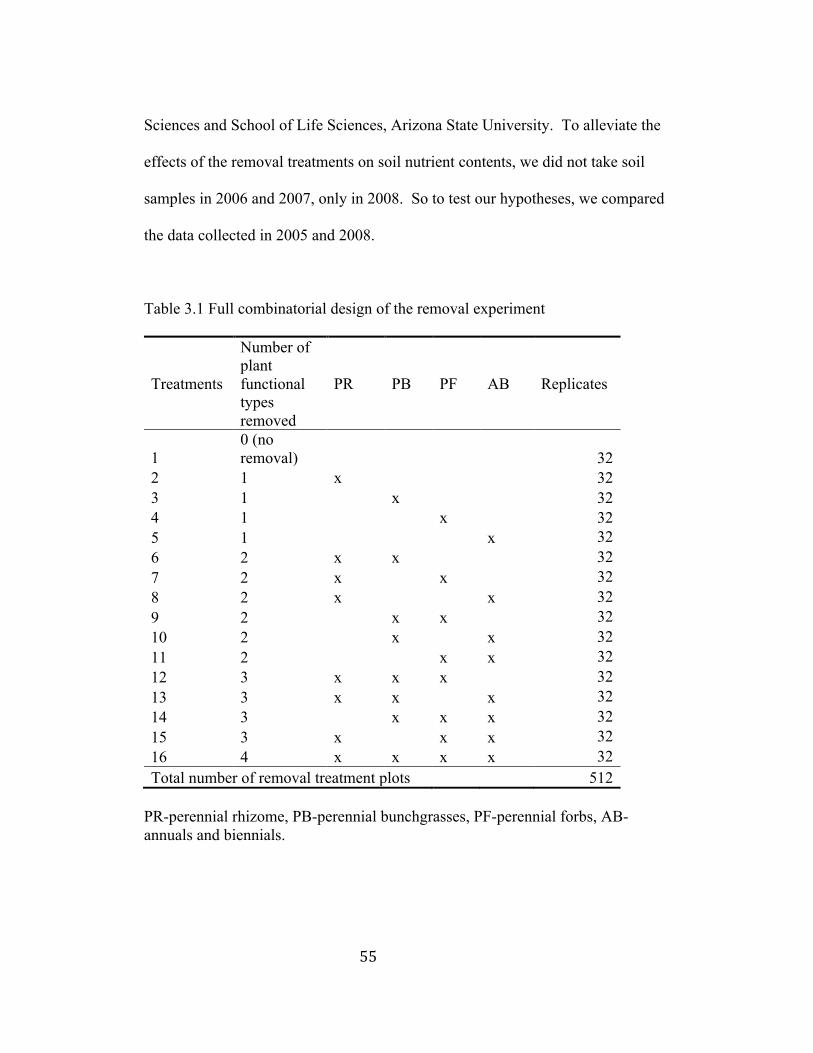
55
Sciences and School of Life Sciences, Arizona State University. To alleviate the
effects of the removal treatments on soil nutrient contents, we did not take soil
samples in 2006 and 2007, only in 2008. So to test our hypotheses, we compared
the data collected in 2005 and 2008.
Table 3.1 Full combinatorial design of the removal experiment
Treatments
Number of plant functional types removed
PR PB PF AB Replicates
1 0 (no removal) 32
2 1 x 32 3 1 x 32 4 1 x 32 5 1 x 32 6 2 x x 32 7 2 x x 32 8 2 x x 32 9 2 x x 32 10 2 x x 32 11 2 x x 32 12 3 x x x 32 13 3 x x x 32 14 3 x x x 32 15 3 x x x 32 16 4 x x x x 32 Total number of removal treatment plots 512
PR-perennial rhizome, PB-perennial bunchgrasses, PF-perennial forbs, AB-annuals and biennials.
56
2.5 Data analysis
We used both traditional statistics and geostatistics to analyze the spatial
characteristics of the measured variables. Traditional statistics, such as mean,
standard deviation, and coefficient of variation (CV), were used to examine the
degree of overall variation.
Semivariograms were used to quantify the spatial structure of the variables
of interest. In a spatial data set, points located closer to each other usually have
values more similar than points far apart. As a result, semivariance will increase
with distance, until the dissimilarity among data points is no longer distance-
dependent. The relationship between semivariance and distance can be fitted with
regression models (e.g., spherical, exponential, Gaussian and linear). The fitted
curve is called a semivariogram, and several parameters can be derived. The
plateau of a semivariogram curve is called sill, the distance from zero to where
the sill occurs is called range, the semivariance at zero distance is called nugget.
Nuggets are often greater than zero because of sampling error or the lack of
observations at very small distances. If a semivariogram does not show
autocorrelation (i.e., sill is equal to nugget), it is defined as a nugget effect (Isaaks
and Srivastava 1989). In this study, we used spatial heterogeneity percentage
(which is defined as 100 (sill−nugget)/sill) to indicate the degree of spatially
structured variability (Rossi et al. 1992, Robertson and Gross 1994, Li and
Reynolds 1995).
57
Correlograms generated from Moran’s I index against lag distances were
also used in our study for the purpose of comparison. Moran’s I, a global
measure of spatial autocorrelation, was also used to identify the degree of spatial
autocorrelation on variables over distances in our study (Moran 1948).
Semivariance and Moran’s I are complementary for evaluating the spatial
structure of data, both of which will be constructed using the GS+ package,
version 7.0 (Gamma Design Software 1999, Plainwell, MI, USA). In our study,
the minimum lag distance was 7 m, which corresponds to the minimal distance
between two adjacent sampled plots, while the maximum lag distance was
extended to 186 m (approximately equals 50% of the distance between the largest
lag pair) (Rossi et al. 1992).
Correlation comparisons among variables in soil nutrients, biodiversity
measures and aboveground biomass collected in 2005 and 2008 were analyzed by
the modified t-test. 82 plots were sampled for variables in TC and TN in both
2005 and 2008, 490 plots for variables in biodiversity measures and aboveground
biomass. The independence of samples could not be guaranteed at such a fine
scale, so the modified t-test correlation was used to correct the degree of freedom,
based on the amount of autocorrelation in the data (Clifford et al. 1989). The
modified t-test was performed using PASSaGE (V. 2.0) software
(http://www.passagesoftware.net/).
After the modified t-test, we identified those variable pairs from
biodiversity measures and aboveground biomass, the relationship of which varied
58
significantly between 2005 and 2008 (e.g, from positive to negative, from positive
to random, and etc.). We did Pearson’s correlation analysis for such variable
pairs under the different complete and partial treatments. The Pearson’s
correlation was analyzed using SAS Version 9.2 (SAS Institute Inc. 2008).
3. Results
3.1 Descriptive summary of BEF variables in 2005 and in 2008
From 2005 to 2008, TC decreased by 57.57%, from 45.91 ± 1.09 g⋅kg-1
averaged over a total of 79 sampled plots to 19.76 ± 0.38 g⋅kg-1over a total of the
same 79 sampled plots (Table 3.2). TN did not vary very much from 2005 to
2008, which decreased only by 14.34% (Table 3.2). Coefficients of variations
(CVs) of HPFT and EPFT increased significantly by 161.80% and 141.48% from
2005 to 2008, respectively (Table 3.2). Aboveground biomass at the levels of
PFT and the whole community also varied dramatically, especially for the annuals
and biennials functional type. In 2005 we did not conduct statistics for the annual
and biennials functional type due to small sample size, whereas in 2008 annuals
and biennials showed up greatly, and the mean value of aboveground biomass of
this functional type was 1.74 ± 2.43 g⋅m-2 (Table 3.2). Large differences for the
aboveground biomass between 2005 and 2008 were also found in CVs, ranging
from 25.97% for AGB to 78.87% for perennial forbs in 2005 versus ranging from
43.69% for AGB to 3097.13% for annuals and biennials in 2008 (Table 3.2).
3.2 Comparison of spatial patterns of soil nutrients, plant diversity and
aboveground biomass between 2005 and 2008 3.2.1 Soil nutrients
59
We used spatial autocorrelation analysis to quantify spatial autocorrelation
among sample points within the field. For TC and TN contents examined in
2005, the resulting semivariograms demonstrated moderate spatial autocorrelation
among sample locations (Table 3.3). The degree of autocorrelation was the
strongest for locations within 77 m of one another for TC, and within 102 m for
TN (Table 3.3, Fig. 3.1 A1 and B1). The values of spatial heterogeneity
percentage were high at 60% and 73% for TC and TN in 2005, suggesting that
much of population variance was a function of spatial autocorrelation (Table 3.3).
The remaining variance was due either to experimental error or to autocorrelation
at the lag distance below 7 m. TC and TN were positively autocorrelated within
60 m, and then showed negative autocorrelation at greater lag distances (Fig. 3.2
A1 and B1).
Spherical model also provided the best fit for TC and TN in 2008 (Table
3.3). Range values were 13 m and 75 m for TC and TN in 2008 (Table 3.3). TC
sampled in 2008 showed a higher spatial autocorrelation represented by the value
of spatial heterogeneity percentage at 97% (Table 3.3), in contrast to the value of
60% in 2005. The semivariogram for TN in 2008 (Fig. 3.1 B2) exhibited a higher
nugget effect compared to TN in 2005 (Fig. 3.1 B1), indicating the variance
among points close to one another was no different than variance among points
farther apart. Correlograms showed that TC demonstrated a periodic
autocorrelation with a positive correlation within 60 m, and a negative correlation
60
at the lag distance between 60 m and 70 m, then repeated this trend with the
increasing lag distances (Fig. 3.2 A2 and B2).
3.2.2 Plant diversity
In 2005, the “best-fit” model was exponential model for both HPFT and
EPFT (Table 3.3, Fig. 3.3 A1, B1). The ranges were 26.60 m and 28.20 m for HPFT
and EPFT, respectively (Table 3.3). The values of spatial heterogeneity percentage
showed that both HPFT and EPFT exhibited a moderate spatial structure (< 75%).
Correlograms showed that these measures were positively autocorrelated within
75 m, and then showed negative autocorrelations and randomness at greater lag
distances (Fig. 3.4 A1, B1).
The plant removal treatment had a significant effect on the spatial
structure of biodiversity measures at the level of plant functional type in 2008
(Table 3.3, Fig. 3.3 A2, B2). Exponential model provided the best fit to
semivariograms for HPFT and EPFT (Table 3.3). The ranges were 14.20 m and 4.90
m for HPFT and EPFT, respectively (Table 3.3). Both of these two variables
exhibited stronger spatial structure in 2008 with the values of spatial
heterogeneity percentage at 91% of population variances, compared to the values
at 67-70% derived in 2005 (Table 3.3). From the correlograms constructed for
biodiversity measures (Fig. 3.4 A2, B2), the pattern for HPFT in 2008 was highly
similar to the one for EPFT in 2008 as both of them were positively autocorrelated

61
within the lag distance of 70 m, and negatively autocorrelated at the distance
between 70 m and 100 m.
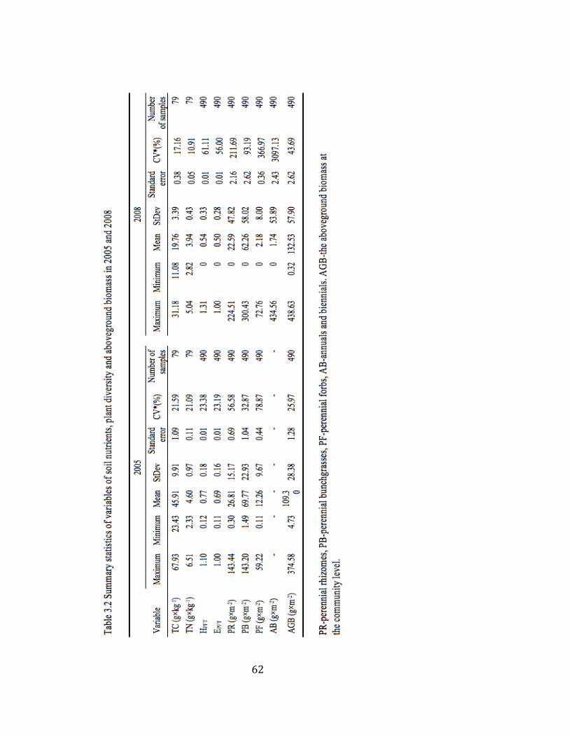
62
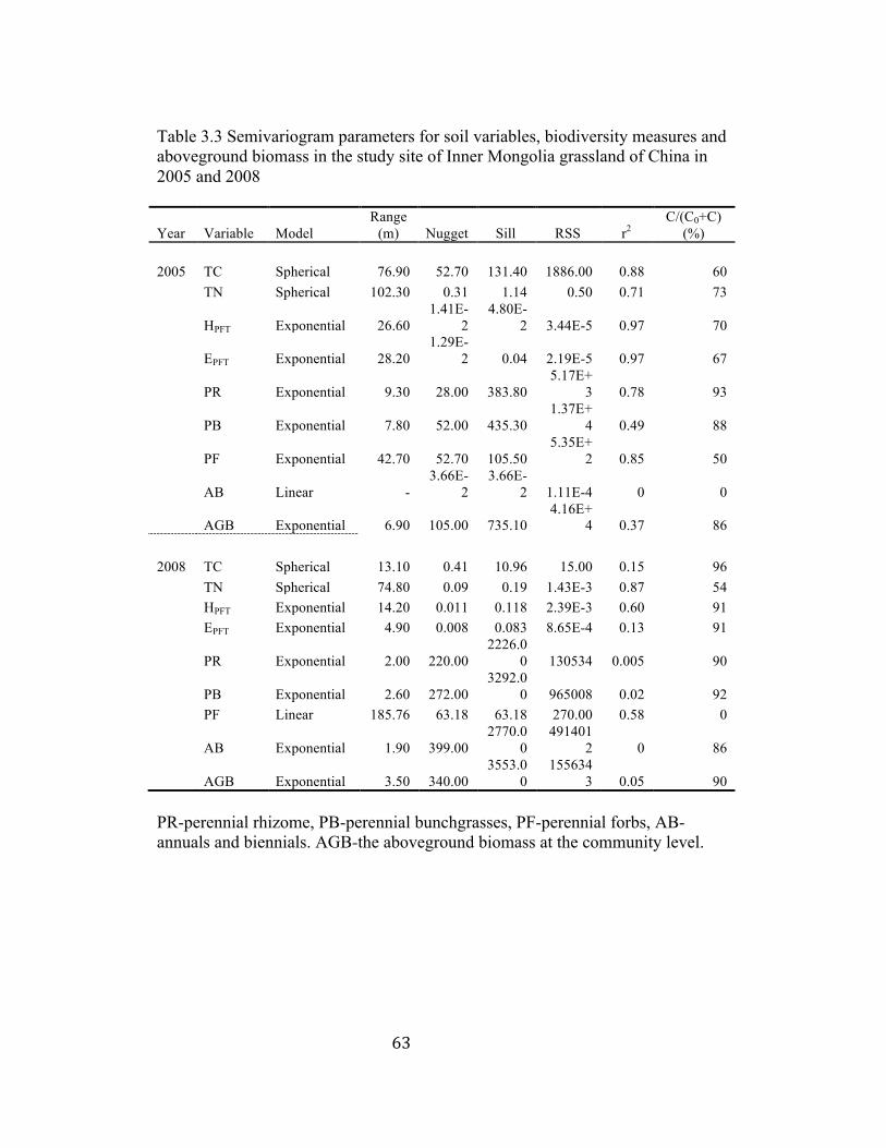
63
Table 3.3 Semivariogram parameters for soil variables, biodiversity measures and aboveground biomass in the study site of Inner Mongolia grassland of China in 2005 and 2008
Year Variable Model Range
(m) Nugget Sill RSS r2 C/(C0+C)
(%)
2005 TC Spherical 76.90 52.70 131.40 1886.00 0.88 60 TN Spherical 102.30 0.31 1.14 0.50 0.71 73
HPFT Exponential 26.60 1.41E-
2 4.80E-
2 3.44E-5 0.97 70
EPFT Exponential 28.20 1.29E-
2 0.04 2.19E-5 0.97 67
PR Exponential 9.30 28.00 383.80 5.17E+
3 0.78 93
PB Exponential 7.80 52.00 435.30 1.37E+
4 0.49 88
PF Exponential 42.70 52.70 105.50 5.35E+
2 0.85 50
AB Linear - 3.66E-
2 3.66E-
2 1.11E-4 0 0
AGB Exponential 6.90 105.00 735.10 4.16E+
4 0.37 86 2008 TC Spherical 13.10 0.41 10.96 15.00 0.15 96 TN Spherical 74.80 0.09 0.19 1.43E-3 0.87 54 HPFT Exponential 14.20 0.011 0.118 2.39E-3 0.60 91 EPFT Exponential 4.90 0.008 0.083 8.65E-4 0.13 91
PR Exponential 2.00 220.00 2226.0
0 130534 0.005 90
PB Exponential 2.60 272.00 3292.0
0 965008 0.02 92 PF Linear 185.76 63.18 63.18 270.00 0.58 0
AB Exponential 1.90 399.00 2770.0
0 491401
2 0 86
AGB Exponential 3.50 340.00 3553.0
0 155634
3 0.05 90 PR-perennial rhizome, PB-perennial bunchgrasses, PF-perennial forbs, AB-annuals and biennials. AGB-the aboveground biomass at the community level.
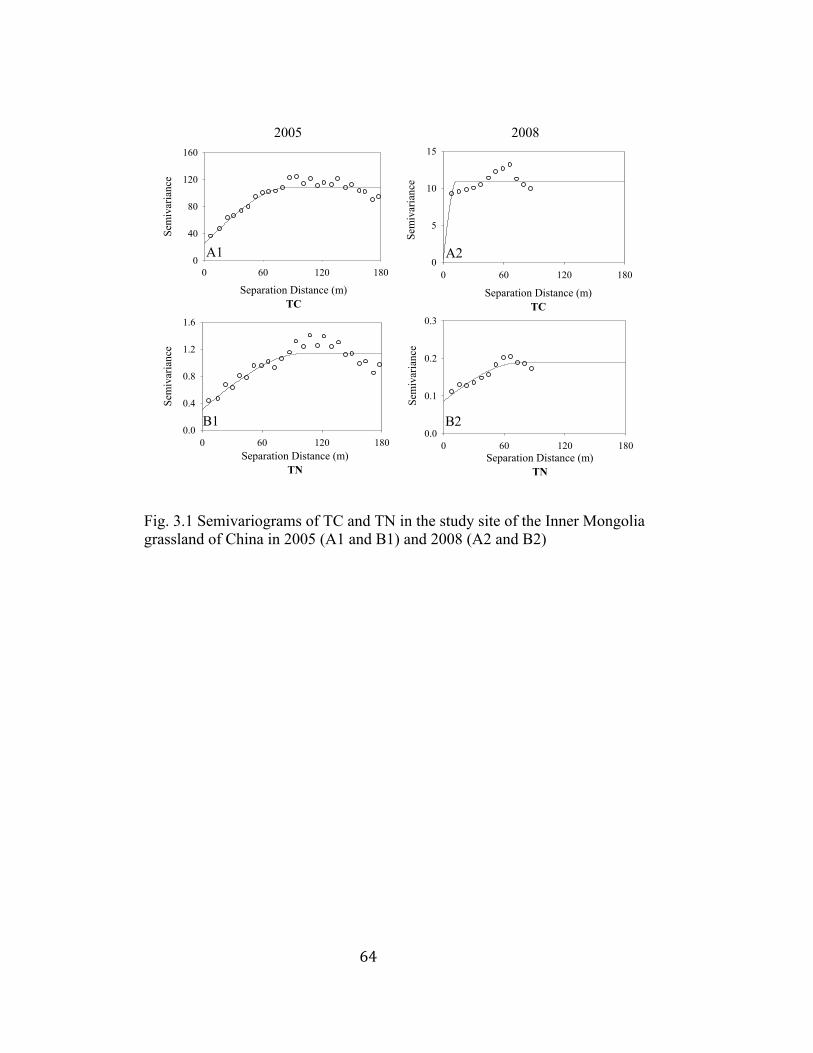
64
0 60 120 1800
5
10
15
Separation Distance (m)TC
0 60 120 180
Sem
ivar
ianc
e
0
40
80
120
160
Separation Distance (m)TN
0 60 120 180
Sem
ivar
ianc
e
0.0
0.4
0.8
1.2
1.6
Separation Distance (m)TC
Separation Distance (m)TN
2005 2008
A1 A2
B1 B20 60 120 180
0.0
0.1
0.2
0.3
B2Se
miv
aria
nce
Sem
ivar
ianc
e
Fig. 3.1 Semivariograms of TC and TN in the study site of the Inner Mongolia grassland of China in 2005 (A1 and B1) and 2008 (A2 and B2)
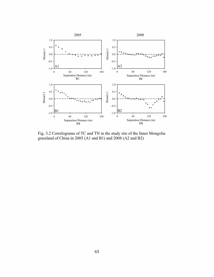
65
Separation Distance (m)TC
0 60 120 180
Mor
an's
I
-1.0
-0.5
0.0
0.5
1.0
Separation Distance (m)TN
0 60 120 180-1.0
-0.5
0.0
0.5
1.0
0 60 120 180
Mor
an's
I
-1.0
-0.5
0.0
0.5
1.0
Separation Distance (m)TN
0 60 120 180
Mor
an's
I
-1.0
-0.5
0.0
0.5
1.0
Separation Distance (m)TC
Mor
an's
I
2005 2008
A1 A2
B1 B2
Fig. 3.2 Correlograms of TC and TN in the study site of the Inner Mongolia grassland of China in 2005 (A1 and B1) and 2008 (A2 and B2)
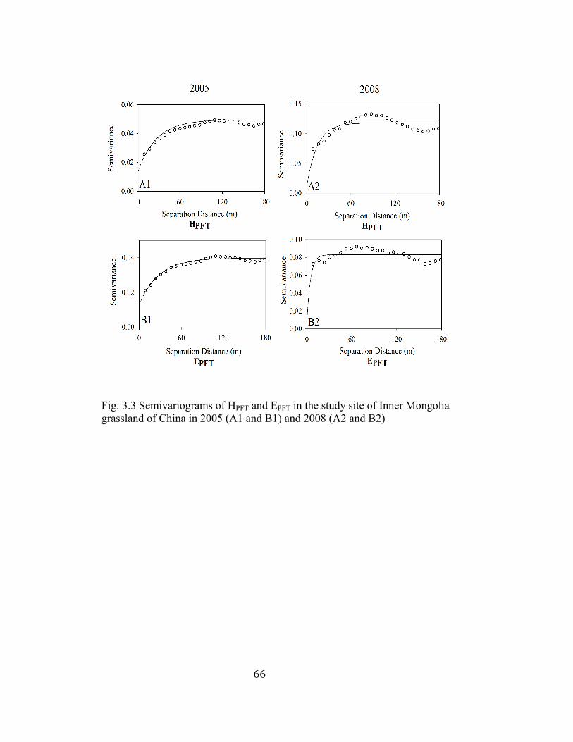
66
Fig. 3.3 Semivariograms of HPFT and EPFT in the study site of Inner Mongolia grassland of China in 2005 (A1 and B1) and 2008 (A2 and B2)
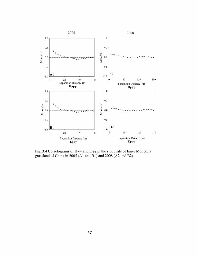
67
Separation Distance (m)HPFT
0 60 120 180
Mor
an's
I
-1.0
-0.5
0.0
0.5
1.0
Separation Disance (m)EPFT
0 60 120 180
Mor
an's
I
-1.0
-0.5
0.0
0.5
1.0
0 60 120 180
Mor
an's
I
-1.0
-0.5
0.0
0.5
1.0
Separation Distance (m)EPFT
0 60 120 180-1.0
-0.5
0.0
0.5
1.0
Separation Distance (m)HPFT
Moran's I
2005 2008
A1 A2
B1 B2
Fig. 3.4 Correlograms of HPFT and EPFT in the study site of Inner Mongolia grassland of China in 2005 (A1 and B1) and 2008 (A2 and B2)
68
3.2.3 Aboveground biomass
In 2005, exponential model was the best fit to the semivariograms for
most aboveground biomass of PFTs (Table 3.3, Fig. 3.5). The PFT of annuals
and biennials with only six samples was better fit by linear model with no range
value detected (Table 3.3, Fig. 3.5 D1). Two dominant PFTs, perennial rhizome
and perennial bunchgrasses, displayed ranges of spatial autocorrelation at 9.30 m
and 7.80 m, respectively, whereas the non-dominant PFT, perennial forbs, had the
range value of 42.70 m (Table 3.3). The values of spatial heterogeneity
percentage were above 50% for perennial rhizome, perennial bunchgrasses and
perennial forbs, indicating higher spatial structures in these plant functional types
(Table 3.3). Correlograms showed that perennial rhizome and perennial
bunchgrasses functional types were positively autocorrelated within 50 m, and
then were randomly distributed with the increasing lag distances (Fig. 3.6 A1 and
B1). The non-dominant PFT, perennial forbs, was positively autocorrelated
within 80 m, and then negatively autocorrelated between 80 m and 150 m (Fig.
3.6 C1). Exponential model provided the best fit to semivariograms of AGB at
the community level (Table 3.3). The range of AGB was 6.90 m and the value of
spatial heterogeneity percentage was 86% at this level (Table 3.3).
In 2008, exponential model was the best fit to the semivariograms for
most aboveground biomass of PFTs, with the exception of perennial forbs fit by
linear model (Table 3.3). The range values for the variables in aboveground
biomass sampled in 2008 decreased (except PF), ranging from 1.90 m for annuals
69
and biennials to 185.76 for perennial forbs, in comparison to the range values of
6.90 m for AGB to 42.70 m for perennial forbs derived from variables of
aboveground biomass sampled in 2005 (Table 3.3). In 2008, perennial forbs did
not show any spatial structure with the value of spatial heterogeneity percentage
at 0%, whereas annuals and biennials exhibited high spatial structure with the
value of spatial heterogeneity percentage at 86% (Table 3.3, Fig. 3.5). The
correlograms showed that there was random autocorrelation for each of the
variables in aboveground biomass at the level of PFT after the removal treatment
in 2008, which was quite different from the pattern showing that those variables
in 2005 before removal treatment exhibited a positive autocorrelation within short
distances apart (Fig. 3.6).
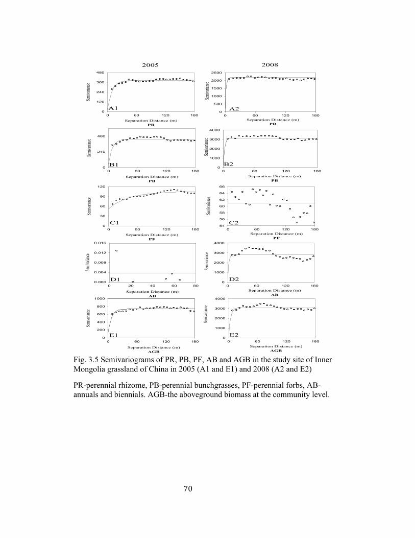
70
0 60 120 1800
1000
2000
3000
4000
0 60 120 1800
500
1000
1500
2000
2500
Separation Distance (m)PR
0 60 120 180
Semiva
riance
0
120
240
360
480
Separation Distance (m)PR
Separation Distance (m)PB
0 60 120 180
Semiva
riance
0
240
480
0 60 120 1800
1000
2000
3000
4000
Separation Distance (m)PF
0 60 120 180
Semiva
riance
0
30
60
90
120
Separation Distance (m)AGB
0 60 120 180
Semiva
riance
0
200
400
600
800
1000
Separation Distance (m)AB
0 20 40 60 80
Semiva
riance
0.000
0.004
0.008
0.012
0.016
0 60 120 18054
56
58
60
62
64
66
0 60 120 1800
1000
2000
3000
4000
Separation Distance (m)PB
Separation Distance (m)AGB
Separation Distance (m)AB
Separation Distance (m)PF
Semiva
riance
Semiva
riance
Semiva
riance
Semiva
riance
Semiva
riance
A1 A2
B1 B2
C1 C2
D1 D2
E1 E2
2005 2008
Fig. 3.5 Semivariograms of PR, PB, PF, AB and AGB in the study site of Inner Mongolia grassland of China in 2005 (A1 and E1) and 2008 (A2 and E2)
PR-perennial rhizome, PB-perennial bunchgrasses, PF-perennial forbs, AB-annuals and biennials. AGB-the aboveground biomass at the community level.
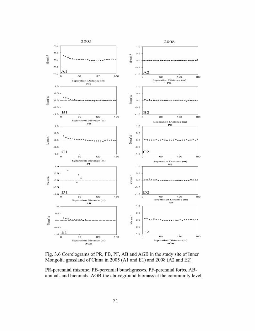
71
0 60 120 180-1.0
-0.5
0.0
0.5
1.0
Separation Distance (m)PR
0 60 120 180
Moran
's I
-1.0
-0.5
0.0
0.5
1.0
Separation Distance (m)PR
Moran
's I
Separation Distance (m)PB
0 60 120 180-1.0
-0.5
0.0
0.5
1.0
Separation Distance (m)PF
0 60 120 180-1.0
-0.5
0.0
0.5
1.0
Separation Distance (m)PB
0 60 120 180
Moran
's I
-1.0
-0.5
0.0
0.5
1.0
Separation Distance (m)PF
0 60 120 180
Moran
's I
-1.0
-0.5
0.0
0.5
1.0
0 60 120 180-1.0
-0.5
0.0
0.5
1.0
Separation Distance (m)AB
0 60 120 180
Moran
's I
-1.0
-0.5
0.0
0.5
1.0
Separation Distance (m)AGB
0 60 120 180
Moran
's I
-1.0
-0.5
0.0
0.5
1.0
0 60 120 180
Moran
's I
-1.0
-0.5
0.0
0.5
1.0
Separation Distance (m)AB
Separation Distance (m)AGB
Moran
's IMo
ran's I
Moran
's I
2005 2008
A1 A2
B1 B2
C1 C2
D1 D2
E1 E2
Fig. 3.6 Correlograms of PR, PB, PF, AB and AGB in the study site of Inner Mongolia grassland of China in 2005 (A1 and E1) and 2008 (A2 and E2)
PR-perennial rhizome, PB-perennial bunchgrasses, PF-perennial forbs, AB-annuals and biennials. AGB-the aboveground biomass at the community level.
72
3.3 Comparing relationships among soil nutrients, biodiversity measures,
and aboveground biomass before and after biodiversity removal
Similar to the relationship between TC and TN found in 2005, the removal
treatment did not affect the relationship between these two variables in 2008, with
a significantly positive correlation (r = 0.829 and P < 0.01). Both TC and TN
were significantly positively correlated (0.314 < r < 0.339; P < 0.01) with HPFT
and EPFT in 2005, however, no correlations were found between variables in soil
nutrients and biodiversity measures in 2008. TC was not correlated with variables
of the aboveground biomass at the levels of PFT and the whole community in
2008, which was different from the findings that there had been a strongly
positive correlation between TC and perennial rhizome (r = 0.238 and P < 0.01),
and between TC and perennial forbs (r = 0.222 and P < 0.05) in 2005. For TN,
there were no correlations with variables in biodiversity and aboveground
biomass in 2008, whereas in 2005 we found that TN was significantly positively
correlated to HPFT (r = 0.314 and P < 0.01), EPFT (r = 0.314 and P < 0.01),
perennial rhizome (r = 0.231 and P < 0.05), and perennial forbs (r = 0.188 and P <
0.05). We did not find any correlations between soil nutrients and aboveground
biomass at the community level either in 2005 or in 2008 (Table 3.4).
For variables of biodiversity measures, plant functional type diversity
(HPFT) was still strongly positively correlated with plant functional type evenness
(EPFT) in 2008 (r = 0.892 and P < 0.01), similar to the correlation between these
two variables in 2005 (r = 1 and P < 0.01). In 2008, HPFT had no correlations with

73
perennial bunchgrasses (r = 0) and AGB (r =-0.012).
Among variables of aboveground biomass at the level of PFT sampled in
2008, we found that strongly negative correlations existed between perennial
rhizome and perennial bunchgrasses (r = -0.434 and P < 0.01), between perennial
rhizome and annuals and biennials (r = -0.182 and P < 0.01), between perennial
bunchgrasses and perennial forbs (r = -0.154 and P < 0.01), and between
perennial bunchgrasses and annuals and biennials (r = -0.285 and P < 0.01). The
phenomenon that no significant correlations were found between perennial
rhizome and perennial forbs, and between perennial forbs and AGB in 2008 did
not occur in 2005, and significantly positive correlations between perennial
rhizome and perennial forbs and between perennial forbs and AGB were detected
in 2005 (r = 0.393 and P < 0.01, and r = 0.415 and P < 0.01, respectively).
Among the four functional types, significantly positive correlations were found
between perennial rhizome and AGB (r = 0.230 and P < 0.01), and between
perennial bunchgrasses and AGB (r = 0.329 and P < 0.01) in 2008, whereas
perennial rhizome, perennial bunchgrasses and perennial forbs all were
significantly positively correlated with AGB in 2005 (Table 3.4).
Based on Table 3.4, we found that the relationships between HPFT and
AGB, between HPFT and perennial bunchgrasses, between perennial forbs and
AGB, and between perennial rhizome and perennial forbs have changed
significantly from 2005 to 2008. So, we did Pearson’s analysis to investigate the
change of the relationship for the above variable pairs under different treatments.
74
Under the complete removals of perennial rhizome and perennial rhizome +
perennial bunchgrasses, and the partial removals of perennial bunchgrasses +
perennial forbs + annuals and biennials, the correlation between HPFT and AGB
changed significantly in 2008, in comparison to those in 2005. For HPFT and
perennial bunchgrasses, the complete removal of perennial forbs made the change
from the significantly negative correlation (r = -0.291, P < 0.01 and n = 16) to no
correlation, and the complete removals of annuals and biennials, perennial
rhizome + annuals and biennials changed the relationship from no correlation in
2005 to significantly negative correlation in 2008.
Because of the complete removal with PB, PR+PB, PB+PR, PB+AB,
PR+PB+PF, PR+PB+AB, PB+PF+AB, and PR+PB+PF+AB, there was no
relationship between HPFT and perennial rhizome in 2008. Several partial
removals also made the change of the relationship between HPFT and perennial
bunchgrasses. The partial removals of perennial bunchgrasses, perennial forbs
and perennial rhizome + perennial bunchgrasses made the change from the
negative correlation in 2005 (-0.783 < r < -0.692) to no correlation in 2008 (Table
3.5).
With the complete removal of perennial rhizome + annuals and biennials,
the correlation of HPFT and perennial bunchgrasses presented significantly
negative (r = -0.862 and P < 0.01) in 2008, compared to no correlation in 2005.
In 2008, the correlation of HPFT and perennial bunchgrasses was nonexistent with
the partial removals of perennial bunchgrasses, perennial forbs and perennial
75
rhizome + perennial bunchgrasses, compared to the negative correlation occurring
in 2005. The partial removal of perennial rhizome + perennial bunchgrasses +
annuals and biennials changed the relationship between HPFT and perennial
bunchgrasses from significantly positive in 2005 to significantly negative in 2008,
and the partial removal of perennial bunchgrasses + perennial forbs + annuals and
biennials inversely changed the relationship, from significantly negative to
significantly positive. The complete removals of perennial rhizome, annuals and
biennials and perennials bunchgrasses + annuals and biennials and the partial
removals of perennial rhizome + perennial bunchgrasses and perennial rhizome +
perennials bunchgrasses + annuals and biennials changed the relationship between
perennial forbs and AGB from significantly positive in 2005 to no correlation in
2008 (Table 3.5).
The complete removals of plant functional types under any treatments did
not change the relationship of perennial rhizome and perennial forbs significantly,
with the exception of those treatments either perennial rhizome or perennial
bunchgrasses being removed. However, the partial removal changed the
correlation of perennial rhizome and perennial forbs significantly. With the
partial removals of PB, PB+AB, and PB+PF+AB, the relationship between
perennial rhizome and perennial forbs changed from no correlation in 2005 to
significantly positive in 2008, and with the partial removals of PF, AB, PR+AB,
and PR+PB+AB, the relationship between perennial rhizome and perennial forbs
changed from significantly positive to no correlation (Table 3.5).
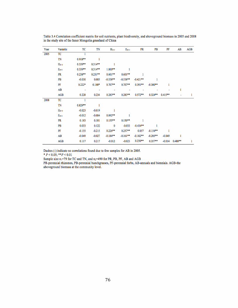
76
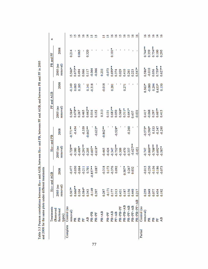
77
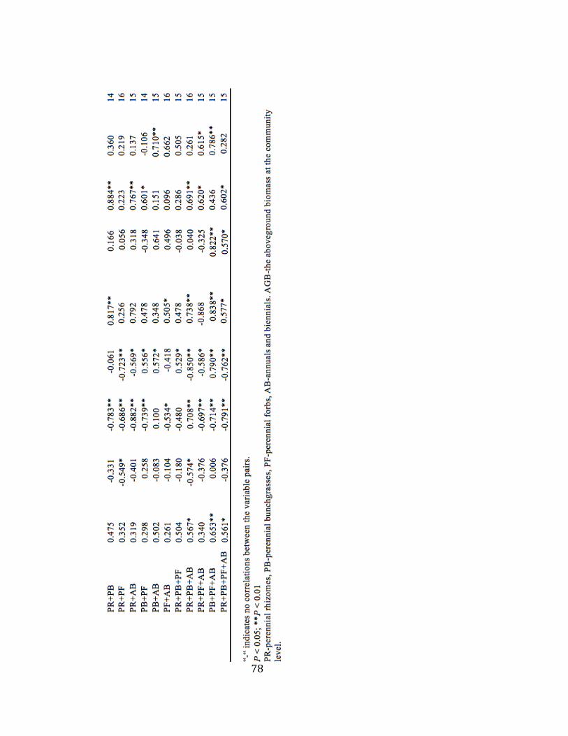
78
79
4 Discussion
4.1 Spatial autocorrelation
We hypothesized that the spatial patterns of most variables representing
biodiversity and ecosystem functioning would be different before the biodiversity
removal (2005) and after (2008). Our results show that the average patch sizes of
TC and TN decreased from 2005 to 2008, and that TC exhibited a higher degree
of spatial autocorrelation and a higher value of spatial heterogeneity percentage
after the biodiversity removal (Table 3.3). Biodiversity measures and
aboveground biomass at the levels of plant functional type and the community in
2008 also decreased in the average patch size and increased in spatial patchiness
due to the biodiversity manipulation (Table 3.3). These differences were
primarily due to the altered spatial patterns of vegetation and soil by the physical
removal of plants in 2006. The effects of the spatial distribution of vegetation on
the spatial pattern of soil nutrients have been well documented (Jackson and
Caldwell 1993a, 1993b, Ryel et al. 1996, Cain et al. 1999). In addition, the
physical activity of pulling out plants during the removal manipulation increased
the degree of soil fragmentation, resulting in decreased average patch sizes for TC
and TN in 2008.
The biodiversity removal had differential effects on plant species of
different abundance. The spatial structure of the two dominant PFTs, the
perennial rhizome and perennial bunchgrasses, was not significantly affected by
the removal treatment. For example, 90% of the population variance (C+C0) for
80
the perennial rhizome was attributable to spatial autocorrelation in 2008, and this
value was 93% in 2005 (Table 3.3). For perennial bunchgrasses, the population
variance was 92% in 2008 and 88% in 2005. The spatial pattern of non-dominant
PFTs (including perennial forbs as well as annuals and biennials), however, was
clearly affected by the removal treatment. For example, perennial forbs showed
no spatial dependence with 0% of the model sample variance in 2008, but a
moderate degree of spatial dependence with 50% of the model sample variance in
2005.
While the degree of spatial dependence for aboveground biomass of
dominant PFTs was little affected by the removal treatment, the distance over
which this spatial dependence was expressed did change substantially between the
two years. With the exception of the perennial forbs, the average patch size
represented by the range value of the semivariogram was shorter in 2008 than in
2005 (Table 3.3). The possible explanation for this difference is again the
fragmentation effect of the removal treatment.
Various studies have attempted to explain spatial patterns in plant and soil
properties because these patterns may be indicative of important ecological
mechanisms (Legendre 1993). For example, the spatial pattern of soil nutrients in
desert ecosystems known as “island of fertility” reflects the spatial distribution of
shrubs (Jackson and Caldwell 1993b, Schlesinger et al. 1996), which drives
patterns of nitrogen cycling, soil respiration and other soil properties (Robertson
et al. 1988, Saetre 1999). Spatial patterns in plant biomass may also be related to
81
spatial patterns in genotypes (Stratton 1994, Bjørnstad et al. 1995). Our study
here indicates that biodiversity removal in BEF studies significantly affect the
spatial patterns of plants and soils in several ways. Whether these altered spatial
patterns would confound the biodiversity effects on ecosystem functioning
deserve future studies.
4.2 Spatial correlations
The removal treatment plays a significant role in changing species
composition and spatial correlations at our study site. We found that the average
aboveground biomass of the functional type of annuals and biennials increased
from 2005 to 2008 (Table 3.2), and this was particularly true in the sampled plots
across the study site (Table 3.2). In the mature L. chinensis-dominant community,
annuals and biennials – r-strategists – are usually inferior to perennial rhizome
and perennial bunchgrasses and forbs in terms of competing for water, nutrients,
and light. Annuals and biennials only germinate after rainfall events, and
complete their life cycle quickly with a large amount of small seeds produced
(Chen and Wang 2000, Chen et al. 2001). However, the removal treatment
created a great number of openings within the community, which allowed annuals
and biennials to flourish. In other words, the life history characteristics (e.g.,
nutrition use strategy and the reproduction times) of the functional type of annuals
and biennials can get adjusted to changing habitat quickly (Yuan et al. 2004).
Thus, these r-strategy species responded to the competition-relaxing event
82
strongly, and produced greater biomass than they did prior to the removal
treatments. As a result, the aboveground biomass of annuals and biennials in
2008 increased significantly after the removal treatments.
Prior to the removal treatment in 2005, there was a positive correlation
between aboveground biomass at the community level (AGB) and plant
functional type diversity (HPFT), but this correlation disappeared in 2008 (Table
3.4). This result suggests that, in mature steppe communities without human
disturbances, biodiversity and ecosystem productivity are positively correlated –
confirming the observation by Bai et al. (2004). However, this positive
correlation between diversity and productivity was disrupted by the removal
treatment in 2006. For instance, in the plots with the complete removal of
perennial rhizome + perennial forbs + annuals and biennials in 2008, only the
functional type of perennial bunchgrasses was left untouched and all other plant
functional types were removed. As a result, the plant cover of perennial
bunchgrasses increased even though the diversity of plant functional types
decreased. Therefore, the aboveground biomass of the functional type of
perennial bunchgrasses was greater after the biodiversity manipulation, which
decoupled the correlation between plant diversity and biomass production (r =
0.267).
The relationship between HPFT and the biomass of perennial bunchgrasses
was significantly negative in 2005, and this relationship also disappeared in 2008
(Table 3.4). Under different removal treatments, we found that the complete
83
removal treatments of plant functional types had a significant effect on the
relationship between HPFT and the functional type of perennial bunchgrasses
(Table 3.5). Specifically, because of the complete removal of perennial
bunchgrasses, no correlations were found between HPFT and the functional type of
perennial bunchgrasses.
There was a positive relationship between the aboveground biomass of
perennial forbs and the community-level aboveground biomass in 2005 (Table
3.4). This indicates that the functional type of perennial forbs contributes
significantly to the aboveground biomass at the community level in natural
conditions. However, the correlation in aboveground biomass between the
functional type of perennial forbs and the entire community disappeared in 2008
(Table 3.4). Through the analysis of the correlation between variables under
different treatments, we found that removal of the perennial rhizome resulted in a
great increase in the aboveground biomass of the perennial bunchgrasses because
of the compensatory interactions between these two functional types (Bai et al.
2004). Similarly, there was no correlation between HPFT and the aboveground
biomass for the treatment plots with the complete removal of the perennial
rhizome (Table 3.5).
In 2005, there was a significantly positive relationship between the
aboveground biomass of perennial rhizome and that of perennial forbs (Table
3.4), which may be partly explained by their similar requirements for resources.
The functional type of perennial rhizome, comprised of L. chinensis only, and

84
perennial forbs both grow better in relatively moist areas in the Inner Mongolia
grassland region (Chen and Wang 2000, Chen et al. 2001). In 2008, no
correlation was found between perennial rhizome and perennial forbs. This
change in the relationship between these two plant functional types is again
attributable to the removal of targeted plants and physical disturbances incurred
during the removal treatment (Table 3.5).
In addition, we found that, in several partial removal treatment plots (e.g.,
removals of perennial bunchgrasses, perennial bunchgrasses + annuals and
biennials, perennial bunchgrasses + perennial forbs + annuals and biennials), the
relationship between the functional types of perennial rhizome and perennial forbs
was significantly positive in 2008. This further supports our interpretation that
the complete removal treatment altered the correlations between variables of
interest in our study. Whether and how these altered correlations between
variables would significantly affect the BEF experimental results beg future
investigations.
85
CHAPTER 4 CONCLUSION
1 Major research findings Understanding the effects of spatial heterogeneity on the relationship
between biodiversity and ecosystem functioning (BEF) is important for a number
of reasons. Spatial heterogeneity in resources can modulate the strength and
shape of the BEF relationships (Cardinale et al. 2000), and heterogeneity has long
been recognized to promote species coexistence through resource partitioning
(Tilman and Kareiva 1997) and niche regeneration (Wu and Loucks 1995). Also,
the BEF relationships are scale-dependent (Bond and Chase 2002, Chase and
Leibold 2002, Mouquet and Loreau 2003, Harrison et al. 2006) because
heterogeneity itself varies with scale (Weins 1989, Wu and Loucks 1995).
The first step toward understanding the effects of spatial heterogeneity on
the BEF relationships is to quantify spatial heterogeneity of key variables of
biodiversity and ecosystem functioning, and to identify the spatial relationships
among these variables. Toward this end, we used two datasets from the on-going
Inner Mongolia Grassland Removal Experiment to explore the problem of spatial
heterogeneity in relation to BEF research. Specifically, we addressed the
following two research questions:
1) What are the spatial patterns of soil nutrients, plant biodiversity, and
aboveground biomass in a natural grassland community of Inner Mongolia,
China? How are they related spatially?
86
2) How do removal treatments affect the spatial patterns of soil nutrients,
plant biodiversity, and aboveground biomass? Is there any change for their spatial
correlations after removal treatments?
Our results have shown that plants and soil in the typical steppe
community of Inner Mongolia had the following spatial patterns before the
biodiversity removal treatment (in 2005):
1) Most of the selected variables of biodiversity and ecosystem
functioning were spatially autocorrelated. Soil nutrients such as TC, TN and TP
were spatially autocorrelated over a range of 102 m or less, biodiversity measures
over a range of 120 m or less, and most species and plant functional types over a
range of less than 30 m. This suggests that the characteristic scales of spatial
patchiness varied with different kinds of variables.
2) TC, TN, and TP were highly correlated with each other;
3) Species diversity was positively correlated with aboveground biomass
at both the species and PFT levels; and
4) Dominant species, as well as major PFTs, were negatively correlated
with each other, supporting the hypothesis of compensatory interactions (Bai et al.
2004).
However, the biodiversity removal treatment conducted in 2006
significantly altered the spatial patterns of the plant and soil variables and their
correlations. Based on available data from 2005 and 2008, we were able to
quantify these changes in a comprehensive manner. These changes were not
87
always in the same direction. For example, the degree of spatial autocorrelation
increased for TC but decreased for TN from 2005 to 2008. Most variables,
however, showed a higher degree of spatial patchiness after the biodiversity
removal.
Importantly, the spatial correlations between these variables also changed
significantly after the removal treatment. For instance, the functional types of
perennial rhizome and perennial forbs showed a strongly positive correlation in
2005 but no relationship in 2008. Similarly, most of the statistically significant
correlations between variables that existed in natural conditions were disrupted or
destroyed by the complete removal treatment required for the biodiversity
manipulation experiment.
2 Significance and implications
2.1 Importance for BEF research
Most studies of the BEF relationships have been based on field
experiments, which involve direct manipulations of biodiversity levels. In so
doing, plots with different levels of species or functional diversity are created, and
variables of ecosystem functioning are subsequently measured along the
biodiversity gradient. Then, the relationship between biodiversity and ecosystem
functioning can be explored with statistical analysis. All these experiments
assume that spatial heterogeneity in plants and soil resources is either
insignificant or can be averaged out by having replicates. Our study, however,

88
indicates that the spatial patterns of plant and soil variables in natural grassland
communities may be quite different from those in BEF treatment plots. The
relationships between these variables may be even more different.
Our results challenge the common assumption of homogeneity in BEF
experiments. With these findings, we must ask questions about the validity of
many previous and ongoing BEF experiments. For example, as all BEF
experiments inevitably change the spatial patterns of and correlations between
plant and soil variables one way or another, would these changes in spatial
heterogeneity be confounded with the effects of biodiversity on ecosystem
functioning? If so, how? This thesis work does not provide the direct answers to
these questions, but does provide the first direct quantification of these changes in
spatial patterns. In addition, it suggests that future BEF experiments should
explicitly consider these questions. The specific findings of this study will be
considered in the final analysis of the experimental results from the IMGRE
project – the largest grassland BEF experiment of the world.
2.2 Implications for grassland management
Spatial heterogeneity is critically important to biodiversity and ecosystem
functioning in natural ecosystems, and has been considered fundamental for
biological conservation and ecosystem management (Wu and Loucks 1995,
Pickett et al. 1997, Wu and Hobbs 2007). Grasslands are inherently
heterogeneous because species composition, biodiversity and productivity all vary
89
across multiple scales in addition to grazing activities by herbivores (Wu and
Levin 1994, Ludwig and Tongway 1995, Patten and Ellis 1995, Bai et al. 2007,
2008). Studies have shown that grazing can affect the spatial heterogeneity of
vegetation (Glenn et al. 1992, Rietkerk et al. 2000, Olofsson et al. 2008) and the
spatial patterns of soil nutrients through tramping and wallowing (Knapp et al.
1999).
The results of this study have two major implications for grassland
management. The first is that the lost of biodiversity may lead to altered spatial
patterns of plants and soil as well as the changed relationships between
biodiversity and ecosystem functioning. Previous studies from the region (e.g.,
Bai et al. 2004, 2007, 2008) have shown that high levels of biodiversity, primary
production, and ecosystem stability are positively correlated in the Inner
Mongolia steppe communities. Thus, maintaining a high level of plant diversity
should be a primary goal of the grassland management in this area. Second, our
study shows that the spatial heterogeneity of plants and soil resources in
undisturbed mature grasslands in Inner Mongolia has unique patterns which is
quite different from that after biodiversity loss or disturbances. This suggests that,
to sustain the structure and function of the Inner Mongolia grassland, a second
primary goal of management is to maintain the fine-scale patterns of plants and
soil.
How can these management goals be achieved? Numerous studies have
suggested that managing grazing activities (especially stocking rates) is the key
90
(e.g., Jiang et al. 2006). In the Inner Mongolia grassland, grazing by sheep has
been a major activity that influences spatial heterogeneity of plants and soil and in
turn strongly affects ecosystem processes. Heavy grazing of sheep can decrease
the heterogeneity of plant production and soil nutrients. Thus, maintaining a
moderate level of grazing in rangeland management is essential for preserving
plant biodiversity and fine-scale heterogeneity of plants and soil resources.
In most natural and managed grasslands, a common management goal is to
maintain diversity and productivity (Guo 2007). Although in some grasslands the
management goal is to increase productivity only in order to meet increasing
human demands, this notion is now changing as more people recognize the
importance of nutritional diversity and forage quality (Parton and Risser 1979,
Marriott et al. 2004). It has been widely recognized that varying the frequency,
intensity, and timing of grazing and fires can often increase habitat productivity
and species diversity (Dyer et al. 1991).
91
REFERENCES
Chapter1
Aarssen, L. 1997. High productivity in grassland ecosystems: Effected by species diveristy or productive species? Oikos 80:183.
Bai, Y., X. Han, J. Wu, Z. Chen, and L. Li. 2004. Ecosystem stability and
compensatory effects in the Inner Mongolia Grassland. Nature 431:181-184.
Bai, Y., J. Wu, Q. Pan, J. Huang, Q. Wang, F. Li, A. Buyantuyev, and X. Han.
2007. Positive linear relationship between productivity and diversity: Evidence from the Eurasian Steppe. Journal of Applied Ecology 44:1023-1034.
Bailey, D., R. Billeter, S. Aviron, O. Schweiger, and F. Herzog. 2007. The
influence of thematic resolution on metric selection for biodiversity monitoring in agricultural landscapes. Landscape Ecology 22:461-473.
Campbell, V., G. Murphy, and T. N. Romanuk. 2011. Experimental design and
the outcome and interpretation of diversity-stability relations. Oikos 120:399-408.
Cardinale, B. J., A. R. Ives, and P. Inchausti. 2004. Effects of species diversity on
the primary productivity of ecosystems: extending our spatial and temporal scales of inference. Oikos 104:437-450.
Cardinale, B. J., D. S. Srivastava, J. E. Duffy, J. P. Wright, A. L. Downing, M.
Sankaran, and C. Jouseau. 2006. Effects of biodiversity on the functioning of trophic groups and ecosystems. Nature 443:989-992.
Cardinale, B. J., K. Nelson, and M. A. Palmer. 2000. Linking species diversity to
the functioning of ecosystems: on the importance of environmental context. Oikos 91:175-183.
Chapin, F. S., E.-D. Schulze, and H. A. Mooney. 1992. Biodiversity and
ecosystem processes. Trends in Ecology & Evolution 7:107-108. Chapin, F. S., B. Walker, and R. Hobbs. 1997. Biotic control over the functioning
of ecosystems. Science 277:500-504.
92
Chapin, F. S., E. S. Zavaleta, V. T. Eviner, R. L. Naylor, P. M. Vitousek, H. L. Reynolds, D. U. Hooper, S. Lavorel, O. E. Sala, S. E. Hobbie, M. C. Mack, and S. Diaz. 2000. Consequences of changing biodiversity. Nature 405:234-242.
Cheng, X., S. An, J. Chen, B. Li, Y. Liu, and S. Liu. 2007. Spatial relationships among species, above-ground biomass, N, and P in degraded grasslands in Ordos Plateau, northwestern China. Journal of Arid Environments 68:652-667.
Chesson, P. 2000. Mechanisms of maintenance of species diversity. Annual
Review of Ecology and Systematics 31:343-366. Christensen, N. L., A. M. Bartuska, J. H. Brown, S. Carpenter, C. D'Antonio, R.
Francis, J. F. Franklin, J. A. MacMahon, R. F. Noss, D. J. Parsons, C. H. Peterson, M. G. Turner, and R. G. Woodmansee. 1996. The report of the Ecological Society of America Committee on the scientific basis for ecosystem management. Ecological applications 6:665-691.
Costanza, R., R. d'Arge, R. de Groot, S. Farber, M. Grasso, B. Hannon, K.
Limburg, S. Naeem, R. V. O'Neill, J. Paruelo, R. G. Raskin, P. Sutton, and M. van den Belt. 1997. The value of the world's ecosystem services and natural capital. Nature 387:253-260.
Curran, P. J. 1988. The semivariogram in remote sensing: An introduction.
Remote Sensing of Environment 24:493-507. Daily, G. C., S. Alexander, P. R. Ehrlich, L. Goulder, J. Lubchenco, P. A. Matson,
H. A. Mooney, S. Postel, S. H. Schneider, D. Tilman, and G. M. Woodwell. 1997. Ecosystem services: Benefits supplied to human societies by natural ecosystems. Issues in Ecology 2.
Deutschman, D. H. 2001. Design and analysis of biodiversity field experiments.
Ecological Research 16:833-843. Duffy, J. E. 2009. Why biodiversity is important to the functioning of real-world
ecosystems. Frontiers in Ecology and Environment 7:437-444. Fox, J. W. 2005. Interpreting the 'selection effect' of biodiversity on ecosystem
function. Ecology Letters 8:846-856. Fridley, J. D. 2002. Resource availability dominates and alters the relationship
between species diversity and ecosystem productivity in experimental plant communities. Oecologia 132:271-277.
93
Gaston, K. J. 1996. Species-range-size distributions: Patterns, mechanisms and implications. Trends in Ecology & Evolution 11:197-201.
Gravel, D., T. Bell, C. Barbera, T. Bouvier, T. Pommier, P. Venail, and N.
Mouquet. 2011. Experimental niche evolution alters the strength of the diversity-productivity relationship. Nature 469:89-92.
Grace, J. B., T. M. Anderson, M. D. Smith, E. Seabloom, S. J. Andelman, G. Meche, E. Weiher, L. K. Allain, H. Jutila, M. Sankaran, J. Knops, M. Ritchie, and M. R. Willig. 2007. Does species diversity limit productivity in natural grassland communities? Ecology Letters 10:680-689.
Griffin, J. N., S. R. Jenkins, L. Gamfeldt, D. Jones, S. J. Hawkins, and R. C.
Thompson. 2009. Spatial heterogeneity increases the importance of species richness for an ecosystem process. Oikos 118:1335-1342.
Guo, Q., T. Shaffer, and T. Buhl. 2006. Community maturity, species saturation
and the variant diversity-productivity relationships in grasslands. Ecology Letters 9:1284-1292.
Hector, A. and R. Bagchi. 2007. Biodiversity and ecosystem multifunctionality.
Nature 448:188-190. Hooper, D. U., F. S. Chapin III, J. J. Ewel, A. Hector, P. Inchausti, S. Lavorel, J.
H. Lawton, D. M. Lodge, M. Loreau, S. Naeem, B. Schmid, H. Setala, A. J. Symstad, J. Vandermeer, and D. A. Wardle. 2005. Effects of biodiversity on ecosystem functioning: A consensus of current knowledge. Ecological Monographs 75:3-35.
Huston, M. A. 1997. Hidden treatments in ecological experiments: Re-evaluating
the ecosystem function and biodiversity. Oecologia 110:449-460. Hutchings, J. A. 2000. Collapse and recovery of marine fishes. Nature 406:882-
885. Hutchings, M. J., E. A. John, and A. J. A. Stewart. 2000. The Ecological
Consequences of Environmental Heterogeneity. Blackwell Science, Cambridge, UK.
Ives, A. R. and S. R. Carpenter. 2007. Stability and diversity of ecosystems.
Science 317:58-62. Kolasa, J. and S. T. A. Pickett, editors. 1991. Ecological Heterogeneity. Springer-
Verlag, New York, US.
94
Lechmere-Oertel, R. G., G. I. H. Kerley, and R. M. Cowling. 2005. Patterns and implications of transformation in semi-arid succulent thicket, South Africa. Journal of Arid Environments 62:459-474.
Loreau, M. 2000. Biodiversity and ecosystem functioning: Recent theoretical
advances. Oikos 91:3-17. Loreau, M., S. Naeem, P. Inchausti, J. Bengtsson, J. P. Grime, A. Hector, D. U.
Hooper, M. A. Huston, D. Raffaelli, B. Schmid, D. Tilman, and D. A. Wardle. 2001. Biodiversity and ecosystem functioning: Current knowledge and future challenges. Science 294: 804-808.
Loreau, M., A. Downing, M. C. Emmerson, A. Gonzalez, J. Hughes, P. Inchausti,
J. Joshi, J. Norberg, and O. E. Sala. 2002. A new look at the relationship between diversity and stability. Pages 79-91 in M. Loreau, S. Naeem, and P. Inchausti, editors. Biodiversity and Ecosystem Functioning: Synthesis and Perspectives. Oxford University Press, Oxford, UK.
McCann, K. S. 2000. The diversity-stability debate. Nature 405:228-233. Meisel, J. E. and M. G. Turner. 1998. Scale detection in real and artificial
landscapes using semivariance analysis. Landscape Ecology 13:347-362. Mooney, H. A. 2002. The debate on the role of biodiversity in ecosystem
functioning. Pages 12-17 in M. Loreau, S. Naeem, and P. Inchausti, editors. Biodiversity and Ecosystem Functioning. Oxford University Press, New York, US.
Naeem, S., D. E. Bunker, A. Hector, M. Loreau, and C. Perrings, editors. 2009.
Biodiversity, Ecosystem Functioning, and Human Wellbeing: An Ecological and Economic Perspective. Oxford University Press, New York, US.
Naeem, S., L. J. Thompson, S. P. Lawler, J. H. Lawton, and R. M. Woodfin. 1994.
Declining biodiversity can alter the performance of ecosystems. Nature 368:734-736.
Omenn, G. S. 2006. Presidential Address: Grand challenges and great
opportunities in science, technology, and public policy. Science 314:1696-1704.
Pachepsky, E., J. L. Bown, A. Eberst, U. Bausenwein, P. Millard, G. R. Squire,
and J. W. Crawford. 2007. Consequences of intraspecific variation for the
95
structure and function of ecological communities Part 2: Linking diversity and function. Ecological Modelling 207:277-285.
Pickett, S. T. A. and M. L. Cadenasso. 1995. Landscape ecology: Spatial
heterogeneity in ecological systems. Science 269:331-334. Purvis, A. and A. Hector. 2000. Getting the measure of biodiversity. Nature
405:212-219. Roscher, C., V. M. Temperton, N. Buchmann, and E.-D. Schulze. 2009.
Community assembly and biomass production in regularly and never weeded experimental grasslands. Acta Oecologica 35:206-217.
Spehn, E. M., A. Hector, J. Joshi, M. Scherer-Lorenzen, B. Schmid, E. Bazeley-
White, C. Beierkuhnlein, M. C. Caldeira, M. Diemer, P. G. Dimitrakopoulos, J. A. Finn, H. Freitas, P. S. Giller, J. Good, R. Harris, P. Hogberg, K. Huss-Danell, A. Jumpponen, J. Koricheva, P. W. Leadley, M. Loreau, A. Minns, C. P. H. Mulder, G. O'Donovan, S. J. Otway, C. Palmborg, J. S. Pereira, A. B. Pfisterer, A. Prinz, D. J. Read, E.-D. Schulze, A.-S. D. Saiamantziouras, A. C. Terry, A. Y. Troumbis, F. I. Woodward, S. Yachi, and J. H. Lawton. 2005. Ecosystem effects of biodiversity manipulations in European grasslands. Ecological Monographs 75:37-63.
Tilman, D. 1996. Biodiversity: Population versus ecosystem stability. Ecology
77:350-363. Tilman, D. 1999. The ecological consequences of changes in biodiversity: A
search for general principles. Ecology 80:1455-1474. Tilman, D. 2000. Causes, consequences and ethics of biodiversity. Nature
405:208-211. Tilman, D., C. L. Lehman, and K. T. Thomson. 1997. Plant diversity and
ecosystem productivity: theoretical considerations. Proceedings of the National Academy of Sciences (USA) 94:1857-1861.
Tilman, D., P. B. Reich, J. Knops, D. Wedin, T. Mielke, and C. Lehman. 2001.
Diversity and productivity in a long-term grassland experiment. Science 294:843-845.
Turner, M. G. and J. A. Cardille. 2007. Spatial heterogeneity and ecosystem
processes. Pages 62-77 in J. Wu and R. Hobbs, editors. Key Topics in Landscape Ecology. Cambridge University Press, Cambridge, UK.
96
Wacker, L., O. Baudois, S. Eichenberger-Glinz, and B. Schmid. 2008.
Environmental heterogeneity increases complementarity in experimental grassland communities. Basic and Applied Ecology 9:467-474.
Wardle, D. A. and O. Zackrisson. 2005. Effects of species and functional group
loss on island ecosystem properties. Nature 435:806-810. Whittaker and S. A. Levin. 1975. On the reasons for distinguishing "Niche,
habitat, and ecotope". America Nature 109:79-82. Wilson, E. O. 1988. Biodiversity. National Academy Press, Washington, D.C.,
US. Wilson, E. O. 1993. Diversity of Life. Harvard University Press, Cambridge, MA,
US. Wu, J. and O. L. Loucks. 1995. From balance-of-nature to hierarchical patch
dynamics: A paradigm shift in ecology. Quarterly Review of Biology 70:439-466.
Wu, J. , D. E. Jelinski, M. Luck, and P. T. Tueller. 2000. Multiscale analysis of
landscape heterogeneity: Scale variance and pattern metrics. Geographic Information Sciences 6:6-19.
Yachi, S. and M. Loreau. 1999. Biodiversity and ecosystem productivity in a
fluctuating environment: The insurance hypothesis. Proceedings of the National Academy of Sciences (USA) 96:1463-1468.
Zhang, Q. and D. Zhang. 2006. Resource availability and biodiversity effects on
the productivity, temporal variability and resistance of experimental algal communities. Oikos 114:385-396.
Chapter 2 Augustine, D. J. and D. A. Frank. 2001. Effects of migratory grazers on spatial
heterogeneity of soil nitrogen properties in a grassland ecosystem. Ecology 82:3149-3162.
Bai, Y., X. Han, J. Wu, Z. Chen, and L. Li. 2004. Ecosystem stability and
compensatory effects in the Inner Mongolia grassland. Nature 431:181-184.
97
Bai, Y., J. Wu, Q. Pan, J. Huang, Q. Wang, F. Li, A. Buyantuyev, and X. Han. 2007. Positive linear relationship between productivity and diversity: Evidence from the Eurasian steppe. Journal of Applied Ecology 44:1023-1034.
Bond, E. M. and J. M. Chase. 2002. Biodiversity and ecosystem functioning at
local and regional spatial scales. Pages 467-470. Burrough, P. A. 1995. Spatial aspects of ecological data. Pages 213-265 in R. H.
G. Jongman, C. J. F. ter Braak, and O. F. R. Van Tongeren, editors. Data Analysis in Community and Landscape Ecology. Cambridge University Press, Cambridge, UK.
Chase, J. M. and M. A. Leibold. 2002. Spatial scale dictates the productivity-
biodiversity relationship. Nature 416:427-430. Cheng, X., S. An, J. Chen, B. Li, Y. Liu, and S. Liu. 2007. Spatial relationships
among species, above-ground biomass, N, and P in degraded grasslands in Ordos Plateau, northwestern China. Journal of Arid Environments 68:652-667.
Clifford, P., S. Richardson, and D. Hémon. 1989. Assessing the significance of
the correlation between two spatial processes. Biometrics 45:123-134. Colwell, R. K. and J. A. Coddington. 1995. Estimating terrestrial biodiversity
through extrapolation. Pages 101-119 in D. L. Hawksworth, editor. Biodiversity Measurement and Estimation. Chapman and Hall, London, UK.
David, M. 1977. Geostatistical Ore Reserve Estimation. Elsevier Scientific, New
York, US. Davies, K. F., P. Chesson, S. Harrison, B. D. Inouye, B. A. Melbourne, and K. J.
Rice. 2005. Spatial heterogeneity explains the scale dependence of the native-exotic diversity relationship. Ecology 86:1602-1610.
De Jager, N. R. and J. Pastor. 2009. Declines in moose population density at Isle
Royle National Park, MI, USA and accompanied changes in landscape patterns. Landscape Ecology 24:1389-1403.
Don, A., J. Schumacher, M. Scherer-Lorenzen, T. Scholten, and E. D. Schulze.
2007. Spatial and vertical variation of soil carbon at two grassland sites: Implications for measuring soil carbon stocks. Geoderma 141:272-282.
98
Fortin, M.-J. and M. R. T. Dale. 2005. Spatial Analysis: A Guide for Ecologists. Cambridge University Press, Cambridge, UK.
Gaston, K. J. 2000. Global patterns in biodiversity. Nature 405:220-207. Gross, K., K. Pregitzer, and A. J. Burton. 1995. Spatial variation in nitrogen
availability in three successional plant communities. Journal of Ecology 83:357-367.
He, Z. B., W. Z. Zhao, and X. L. Chang. 2007. The modifiable areal unit problem
of spatial heterogeneity of plant community in the transitional zone between oasis and desert using semivariance analysis. Landscape Ecology 22:95-104.
Hector, A. and R. Hooper. 2002. Darwin and the first ecological experiment.
Science 295:639-640. Hector, A., J. Joshi, M. Scherer-Lorenzen, B. Schmid, E. M. Spehn, L. Wacker,
M. Weilenmann, E. Bazeley-White, C. Beierkuhnlein, M. C. Caldeira, P. G. Dimitrakopoulos, J. A. Finn, K. Huss-Danell, A. Jumpponen, P. W. Leadley, M. Loreau, C. P. H. Mulder, C. Nesshoover, C. Palmborg, D. J. Read, A. S. D. Siamantziouras, A. C. Terry, and A. Y. Troumbis. 2007. Biodiversity and ecosystem functioning: Reconciling the results of experimental and observational studies. Functional Ecology 21:998-1002.
Hector, A., B. Schmid, C. Beierkuhnlein, M. C. Caldeira, M. Diemer, P. G.
Dimitrakopoulos, J. A. Finn, H. Freitas, P. S. Giller, J. Good, R. Harris, P. Hogberg, K. Huss-Dannell, J. Joshi, A. Jumpponen, C. Korner, P. W. Leadley, M. Loreau, A. Minns, C. P. H. Mulder, G. O'Donovan, S. J. Otway, J. S. Pereira, A. Prinz, D. J. Read, M. Scherer-Lorenzen, E.-D. Schulze, A.-S. D. Siamantziouras, E. M. Spehn, A. C. Terry, A. Y. Troumbis, F. I. Woodward, S. Yachi, and J. H. Lawton. 1999. Plant diversity and productivity experiments in European grasslands. Science 286:1123-1127.
Holland, J. D., D. G. Bert, and L. Fahrig. 2004. Determining the spatial scale of
species’ response to habitat. BioScience 54:227-233. Hooper, D. U., F. S. Chapin III, J. J. Ewel, A. Hector, P. Inchausti, S. Lavorel, J.
H. Lawton, D. M. Lodge, M. Loreau, S. Naeem, B. Schmid, H. Setala, A. J. Symstad, J. Vandermeer, and D. A. Wardle. 2005. Effects of biodiversity on ecosystem functioning: A consensus of current knowledge. Ecological Monographs 75:3-35.
99
Hooper, D. U., N. Buchmann, V. Degrange, S. M. Diaz, M. Gessner, P. Grime, and et al. 2002. Species diversity, functional diversity and ecosystem functioning. Pages 195-208 in M. Loreau, S. Naeem, and P. Inchausti, editors. Biodiversity and Ecosystem Functioning. Oxford University Press, Oxford, UK.
Huston, M. A. 1997. Hidden treatments in ecological experiments: Re-evaluating
the ecosystem function and biodiversity. Oecologia 110:449-460. Hutchings, M. J., E. A. John, and D. K. Wijesinghe. 2003. Toward understanding
the consequences of soil heterogeneity for plant populations and communities. Ecology 84:2322-2334.
Inner Mongolia-Ningxia Integrative Expert Team of the Chinese Academy of
Science. 1985. Vegetation of Inner Mongolia. Science Press, Beijing, China.
Kareiva, P. and U. Wennergren. 1995. Connecting landscape patterns to
ecosystem and population processes. Nature 373:299-302. Kolasa, J. and S. T. A. Pickett, editors. 1991. Ecological Heterogeneity. Springer-
Verlag, New York, US. Legendre, P. and M. J. Fortin. 1989. Spatial pattern and ecological analysis.
Vegetatio 80:107-138. Levin, S. A. 1992. The problem of pattern and scale in ecology. Ecology 73:1943-
1967. Li, H. and J. F. Reynolds. 1995. On definition and quantification of heterogeneity.
Oikos 73:280-284. Loreau, M., S. Naeem, and P. Inchausti, editors. 2002. Biodiversity and
Ecosystem Functioning: Synthesis and Perspectives. Oxford University Press, Oxford, UK.
Matheron, G. 1963. Principles of geostatistics. Ecnonomic Geology 58:1246-1266. McNaughton, S. J. 1977. Diversity and stability of ecological communities: A
comment on the role of empiricism in ecology. American Naturalist 111:515-525.
100
McNaughton, S. J. 1993. Biodiversity and function of grazing systems. Pages 361-383 in H. Mooney and E. Schulze, editors. Biodiversity and Ecosystem Function. Springer-Verlag, Berlin, Germany.
Meisel, J. E. and M. G. Turner. 1998. Scale detection in real and artificial
landscapes using semivariance analysis. Landscape Ecology 13:347-362. Mittelbach, G. G., C. F. Steiner, S. M. Scheiner, K. L. Gross, H. L. Reynolds, R.
B. Waide, M. R. Willig, S. I. Dodson, and L. Gough. 2001. What is the observed relationship between species richness and productivity? Ecology 82:2381-2396.
Moran, P. A. P. 1948. The interpretation of statistical maps. Journal of the Royal
Statistical Society B 10:243-251. Naeem, S., D. E. Bunker, A. Hector, M. Loreau, and C. Perrings, editors. 2009.
Biodiversity, Ecosystem Functioning, and Human Wellbeing: An Ecological and Economic Perspective. Oxford University Press, New York, US.
Naeem, S. and J. P. Wright. 2003. Disentangling biodiversity effects on
ecosystem functioning: deriving solutions to a seemingly insurmountable problem. Ecology Letters 6:567-579.
Naeem, S. and S. B. Li. 1997. Biodiversity enhances ecosystem reliability. Nature
390:507-509. Okin, G. S., N. Mladenov, L. Wang, D. Cassel, K. K. Caylor, S. Ringrose, and S.
A. Macko. 2008. Spatial patterns of soil nutrients in two southern African savannas. Journal of Geophysical Research-Biogeosciences 113.
Oline, D. K. and M. C. Grant. 2002. Scaling patterns of biomass and soil
properties: An empirical analysis. Landscape Ecology 17:13-26. Olofsson, J., C. de Mazancourt, and M. J. Crawley. 2008. Spatial heterogeneity
and plant species richness at different spatial scales under rabbit grazing. Oecologia 156:825-834.
Reynolds, H. L., B. A. Hungate, and C. M. D'Antonio. 1997. Soil heterogeneity
and plant competition in an annual grassland. Ecology 78:2076. Robertson, G. P., J. R. Crum, and B. G. Ellis. 1993. The spatial variability of soil
resources following long-term disturbance. Oecologia 96:451-456.
101
Robertson, G. P. and K. L. Gross. 1994. Assessing the heterogeneity of belowground resources: Quantifying pattern and scale. Pages 237-253 in M. M. Caldwell and R. W. Pearcy, editors. Exploitation of Environmental Heterogeneity by Plants: Ecophysiological Processes Above- and Belowground. Academic Press, San Diego, US.
Robertson, G. P., K. M. Klingensmith, M. J. Klug, E. A. Paul, J. R. Crum, and B.
G. Ellis. 1997. Soil resources, microbial activity, and primary production across an agricultural ecosystem. Ecological Applications 7:158-170.
Roscher, C., V. M. Temperton, M. Scherer-Lorenzen, M. Schmitz, J. Schumacher,
B. Schmid, N. Buchmann, W. W. Weisser, and E.-D. Schulze. 2005. Overyielding in experimental grassland communities - irrespective of species pool or spatial scale. Ecology Letters 8:419-429.
Rosenzweig, M. L. 1995. Species Diversity in Space and Time. Cambridge
University Press, Cambridge, UK. Rossi, R. E., D. J. Mulla, A. G. Journel, and E. H. Franz. 1992. Geostatistical
tools for modeling and interpreting ecological spatial dependence. Ecological Monographs 62:277-314.
Sala, O. E. and A. T. Austin. 2000. Methods of estimating aboveground net
primary productivity. Pages 31-43 in O. E. Sala, R. B. Jackson, M. H.A., and R. W. Howarth, editors. Methods in Ecosystem Science. Springer, New York, USA.
Schlesinger, W. H., J. A. Raikes, A. E. Hartley, and A. F. Cross. 1996. On the
spatial pattern of soil nutrients in desert ecosystems. Ecology 77:364-374. Spehn, E. M., A. Hector, J. Joshi, M. Scherer-Lorenzen, B. Schmid, E. Bazeley-
White, C. Beierkuhnlein, M. C. Caldeira, M. Diemer, P. G. Dimitrakopoulos, J. A. Finn, H. Freitas, P. S. Giller, J. Good, R. Harris, P. Hogberg, K. Huss-Danell, A. Jumpponen, J. Koricheva, P. W. Leadley, M. Loreau, A. Minns, C. P. H. Mulder, G. O'Donovan, S. J. Otway, C. Palmborg, J. S. Pereira, A. B. Pfisterer, A. Prinz, D. J. Read, E.-D. Schulze, A.-S. D. Saiamantziouras, A. C. Terry, A. Y. Troumbis, F. I. Woodward, S. Yachi, and J. H. Lawton. 2005. Ecosystem effects of biodiversity manipulations in European grasslands. Ecological Monographs 75:37-63.
Tilman, D. 1982. Resource Competition and Community Structure. Princeton
University Press, Princeton, US.
102
Tilman, D. 1985. The resource-ratio hypothesis of plant succession. American Naturalist 125:827-852.
Tilman, D. 1999. The ecological consequences of changes in biodiversity: A
search for general principles. Ecology 80:1455-1474. Tilman, D. and J. A. Downing. 1994. Biodiversity and stability in grasslands.
Nature 367:363-365. Tilman, D. and P. Kareiva, editors. 1997. Spatial Ecology: The Role of Space in
Population Dynamics and Interspecific Interactions. Princeton University Press, Princeton, US.
Tilman, D., P. B. Reich, J. Knops, D. Wedin, T. Mielke, and C. Lehman. 2001.
Diversity and productivity in a long-term grassland experiment. Science 294:843-845.
Turner, M. G., R. H. Gardner, and R. V. O'Neill. 2001. Landscape Ecology in
Theory and Practice: Pattern and Process. Springer-Verlag, New York, US.
Turner, S. J., R. V. O’Neill, W. Conley, M. R. Conley, and H. C. Humphries.
1991. Pattern and scale: statistics for landscape ecology. Pages 17-50 in M. G. Turner and R. H. Gardner, editors. Quantitative Methods in Landscape Ecology. Springer-Verlag, New York, US.
Waide, R. B., M. R. Willig, C. F. Steiner, G. Mittelbach, L. Gough, S. I. Dodson,
G. P. Juday, and R. Parmenter. 1999. The relationship between productivity and species richness. Annual Review of Ecology and Systematics 30:257-300.
Wang, H. Q., C. A. S. Hall, J. D. Cornell, and M. H. P. Hall. 2002. Spatial
dependence and the relationship of soil organic carbon and soil moisture in the Luquillo Experimental Forest, Puerto Rico. Landscape Ecology 17:671-684.
Wang, L. X., P. P. Mou, J. H. Huang, and J. Wang. 2007. Spatial heterogeneity of
soil nitrogen in a subtropical forest in China. Plant and Soil 295:137-150. Wu, J. 2004. Effects of changing scale on landscape pattern analysis: Scaling
relations. Landscape Ecology 19:125-138.
103
Wu, J., K. B. Jones, H. Li, and O. L. Loucks, editors. 2006. Scaling and Uncertainty Analysis in Ecology: Methods and Applications. Springer, Dordrecht, The Netherlands.
Wu, J. and O. L. Loucks. 1995. From balance-of-nature to hierarchical patch
dynamics: A paradigm shift in ecology. Quarterly Review of Biology 70:439-466.
Wu, J. and R. Hobbs, editors. 2007. Key Topics in Landscape Ecology.
Cambridge University Press, Cambridge, UK. Wu, J. and S. A. Levin. 1994. A spatial patch dynamic modeling approach to
pattern and process in an annual grassland. Ecological Monographs 64:447-464.
Xin, X., X. Li, G. Yang, and B. Xu. 2002. Spatial heterogeneity of grassland
pattern under grazing and forage condition. Yingyong Shengtai Xuebao 13:449-453.
Zawadzki, J., C. J. Cieszewski, and M. Zasada. 2005a. Semivariogram analysis of
Landsat 5 TM textural data for loblolly pine forests. Journal of Forest Science (Prague) 51:47-59.
Zawadzki, J., C. J. Cieszewski, M. Zasada, and R. C. Lowe. 2005b. Applying
geostatistics for investigations of forest ecosystems using remote sensing imagery. Silva Fennica 39:599-617.
Zhang, X. Y., Y. Y. Sui, X. D. Zhang, K. Meng, and S. J. Herbert. 2007. Spatial
variability of nutrient properties in black soil of northeast China. Pedosphere 17:19-29.
Zhou, Z. Y., O. J. Sun, Z. K. Luo, H. M. Jin, Q. S. Chen, and X. G. Han. 2008.
Variation in small-scale spatial heterogeneity of soil properties and vegetation with different land use in semiarid grassland ecosystem. Plant and Soil 310:103-112.
Zuo, X. A., H. L. Zhao, X. Y. Zhao, Y. R. Guo, J. Y. Yun, S. K. Wang, and T.
Miyasaka. 2009. Vegetation pattern variation, soil degradation and their relationship along a grassland desertification gradient in Horqin Sandy Land, northern China. Environmental Geology 58:1227-1237.
Chapter 3
104
Bai, Y., X. Han, J. Wu, Z. Chen, and L. Li. 2004. Ecosystem stability and compensatory effects in the Inner Mongolia grassland. Nature 431:181-184.
Bai, Y., J. Wu, M. Clark, S. Naeem, Q. Pan, J. Huang, L. Zhang, and X. Han.
2010. Tradeoffs and thresholds in the effects of nitrogen addition on biodiversity and ecosystem functioning: evidence from inner Mongolia Grasslands. Global Change Biology 16:358-372.
Bjørnstad, O. N., A. Iversen, and M. Hansen. 1995. The spatial structure of the
gene pool of a viviparous population of Poa alpina - environmental controls and spatial constraints. Nordic Journal of Botany 15:347-354.
Cain, M. L., S. Subler, J. P. Evans, and M.-J. Fortin. 1999. Sampling spatial and
temporal variation in soil nitrogen availability. Oecologia 118:397-404. Cardinale, B. J., A. R. Ives, and P. Inchausti. 2004. Effects of species diversity on
the primary productivity of ecosystems: Extending our spatial and temporal scales of inference. Oikos 104:437-450.
Chen, Z. & S. Wang. 2000. Typical Steppe Ecosystems of China. Science press,
Beijing, China. Chen, S., H. Zhang, L. Wang, Zhanbula and M. Zhao. 2001. Root Systems of
Grassland Plants in Northern China. Jilin University Press, Changchun, China.
Clifford, P., S. Richardson, and D. Hémon. 1989. Assessing the significance of
the correlation between two spatial processes. Biometrics 45:123-134. Diaz, S., A. J. Symstad, F. S. Chapin III, D. A. Wardle, and L. F. Huenneke.
2003. Functional diversity revealed by removal experiments. Trends in Ecology and Evolution 18:140-146.
Feng, D., Z. Liang, X. Xu, X. Zhang, and L. Shan. 2008. Spatial heterogeneity of
soil nutrients and aboveground biomass in abandoned old-fields of Loess Hilly region in northern Shaanxi, China. Acta Ecologica Sinica 28:13-22.
Gundale, M. J., D. A. Wardle, and M.-C. Nilsson. 2010. Vascular plant removal
effects on biological N fixation vary across a boreal forest island gradient. Ecology 91:1704-1714.
105
Guo, D., P. P. Mou, R. H. Jones, and R. J. Mitchell. 2002. Temporal changes in spatial patterns of soil moisture following disturbance: An experimental approach. Journal of Ecology 90:338-347.
Hooper, D. U. 1998. The role of complementarity and competition in ecosystem
responses to variation in plant diversity. Ecology 79:704-719. Hooper, D. U., F. S. Chapin III, J. J. Ewel, A. Hector, P. Inchausti, S. Lavorel, J.
H. Lawton, D. M. Lodge, M. Loreau, S. Naeem, B. Schmid, H. Setala, A. J. Symstad, J. Vandermeer, and D. A. Wardle. 2005. Effects of biodiversity on ecosystem functioning: A consensus of current knowledge. Ecological Monographs 75:3-35.
Isaaks, E. H. and R. M. Srivastava. 1989. An Introduction to Applied
Geostatistics. Oxford University Press, New York. Jackson, R. B. and M. M. Caldwell. 1993a. The scale of nutrient heterogeneity
around individual plants and its quantification with geostatistics. Ecology 74:612-614.
Jackson, R. B. and M. M. Caldwell. 1993b. Geostatistical patterns of soil
heterogeneity around individual plants. Journal of Ecology 81:683-692. Keitt, T. H., O. N. Bjornstad, P. M. Dixon, and S. Citron-Pousty. 2002.
Accounting for spatial pattern when modeling organism-environment interactions. Ecography 25:616-625.
Knorr, M., S. D. Frey, and P. S. Curtis. 2005. Nitrogen additions and litter
decomposition: A meta-analysis. Ecology 86:3252-3257. Legendre, P. 1993. Spatial autocorrelation: Trouble or new paradigm? Ecology
74:1659-1673. Li, H. and J. F. Reynolds. 1995. On definition and quantification of heterogeneity.
Oikos 73:280-284. McLellan, A. J., R. Law, and A. H. Fitter. 1997. Response of calcareous grassland
plant species to diffuse competition: results from a removal experiment. Journal of Ecology 85:479-490.
Moran, P. A. P. 1948. The interpretation of statistical maps. Journal of the Royal
Statistical Society B 10:243-251.
106
Robertson, G. P., M. A. Huston, F. C. Evans, and J. M. Tiedje. 1988. Spatial variability in a successional plant community: patterns of nitrogen availability. Ecology 69:1517-1524.
Robertson, G. P. and K. L. Gross. 1994. Assessing the heterogeneity of
belowground resources: Quantifying pattern and scale. Pages 237-253 in M. M. Caldwell and R. W. Pearcy, editors. Exploitation of Environmental Heterogeneity by Plants: Ecophysiological Processes Above- and Belowground. Academic Press, San Diego, US.
Rossi, R. E., D. J. Mulla, A. G. Journel, and E. H. Franz. 1992. Geostatistical
tools for modeling and interpreting ecological spatial dependence. Ecological Monographs 62:277-314.
Ryel, R. J., M. M. Caldwell, and J. H. Manwaring. 1996. Temporal dynamics of
soil spatial heterogeneity in sage-brush-wheatgrass steppe during a growing season. Plant and Soil 184:299-309.
Saetre, P. 1999. Spatial patterns of ground vegetation, soil microbial biomass and
activity in a mixed spruce-birch stand. Ecography 22:183-192. Schlesinger, W. H., J. A. Raikes, A. E. Hartley, , and A. F. Cross. 1996. On the
spatial pattern of soil nutrients in desert ecosystems. Ecology 77:364-374. Schroeer, A. E., R. L. Hendrick, and T. B. Harrington. 1999. Root, ground cover,
and litterfall dynamics within canopy gaps in a slash pine (Pinus elliottii Engelm.) dominated forest. Ecoscience 6:548-555.
Schulze, A. P. and H. A. Mooney. 1993. Ecosystem Function and Biodiversity.
Springer, Berlin, Germany. Seastedt, T. R., J. M. Briggs, and D. J. Gibson. 1991. Controls of nitrogen
limitation in trallgrass prairie. Oecologia 87:72-79. Silver, W. L. and K. A. Vogt. 1993. Fine root dynamics following single and
multiple disturbances in a subtropical wet forest ecosystem. Journal of Ecology 81:729-738.
Stratton, D. A. 1994. Genotype-by-environment interactions for fitness of
Erigeron annuus show fine-scale selective heterogeneity. Evolution 48:1607-1618.
Wang, H. Q., C. A. S. Hall, J. D. Cornell, and M. H. P. Hall. 2002. Spatial
dependence and the relationship of soil organic carbon and soil moisture
107
in the Luquillo Experimental Forest, Puerto Rico. Landscape Ecology 17:671-684.
Wardle, D. A., K. I. Bonner, G. M. Barker, G. W. Yeates, K. S. Nicholson, R. D.
Bardgett, R. N. Watson, and A. Ghani. 1999. Plant removals in perennial grassland: vegetation dynamics, decomposers, soil biodiversity, and ecosystem properties. Ecological Monographs 69:535-568.
Wilson, E. O., editor. 1988. Biodiversity. National Academy Press, Washington,
D.C., US. Yuan, Z., L. Li, and X. Han. 2004. Nitrogen use efficiency of competing
individuals in a dense stand of an annual herb, Chenopodium Album. 28: 294-299.
Chapter 4
Bai, Y., X. Han, J. Wu, Z. Chen, and L. Li. 2004. Ecosystem stability and compensatory effects in the Inner Mongolia Grassland. Nature 431:181-184.
Bai, Y., J. Wu, Q. Pan, J. Huang, Q. Wang, F. Li, A. Buyantuyev, and X. Han.
2007. Positive linear relationship between productivity and diversity: evidence from the Eurasian Steppe. Journal of Applied Ecology 44:1023-1034.
Bai, Y., J. Wu, Q. Xing, Q. Pan, J. Huang, D. Yang, and X. Han. 2008. Primary
production and rain use efficiency across a precipitation gradient on the Mongolia plateau. Ecology 89:2140-2153.
Bond, E. M. and J. M. Chase. 2002. Biodiversity and ecosystem functioning at
local and regional spatial scales. Ecology Letters 5:467-470. Cardinale, B. J., K. Nelson, and M. A. Palmer. 2000. Linking species diversity to
the functioning of ecosystems: on the importance of environmental context. Oikos 91:175-183.
Chase, J. M. and M. A. Leibold. 2002. Spatial scale dictates the productivity-
biodiversity relationship. Nature 416:427-430. Dyer, M. I., C. L. Turner, and T. R. Seastedt. 1991. Mowing and Fertilization
Effect on Productivity and Spectral Reflectance in Bromus Inermis Plots. Ecological Applications 1:443-452.
108
Glenn, S. M., S. L. Collins, and D. J. Gibson. 1992. Disturbances in tallgrass prairie - Local and regional effects on community heterogeneity. Landscape Ecology 7:243-251.
Guo, Q. 2007. The diversity-biomass-productivity relationships in grassland
management and restoration. Basic and Applied Ecology 8:199-208. Harrison, S., H. D. Safford, J. B. Grace, J. H. Viers, and K. F. Davies. 2006.
Regional and local species richness in an insular environment: Serpentine plants in California. Ecological Monographs 76:41-56.
Jiang, G., X. Han, and J. Wu. 2006. Restoration and management of the Inner
Mongolia Grassland requires a sustainable strategy. AMBIO 35:269-270. Knapp, A. K., J. M. Blair, J. M. Briggs, S. L. Collins, D. C. Hartnett, L. C.
Johnson, and E. G. Towne. 1999. The keystone role of bison in north American tallgrass prairie - Bison increase habitat heterogeneity and alter a broad array of plant, community, and ecosystem processes. Bioscience 49:39-50.
Ludwig, J. A. and D. J. Tongway. 1995. Spatial organisation of landscapes and its
function in semi-arid woodlands, Australia. Landscape Ecology 10:51-63. Marriott, C. A., M. Fothergill, B. Jeangros, M. Scotton, and F. Louault. 2004.
Long-term impacts of extensification of grassland management on biodiversity and productivity in upland areas. A review. Agronomie 24:447-462.
Mouquet, N. and M. Loreau. 2003. Community patterns in source-sink
metacommunities. American Naturalist 162:544-557. Olofsson, J., C. de Mazancourt, and M. J. Crawley. 2008. Spatial heterogeneity
and plant species richness at different spatial scales under rabbit grazing. Oecologia 156:825-834.
Parton, W. J. and P. G. Risser. 1979. Simulated impact of management practices
upon the tallgrass prairie.in N. R. French, editor. Perspectives in Grassland Ecology, Ecological Studies, Vol. 32. Springer, New York, US.
Patten, R. S. and J. E. Ellis. 1995. Patterns of species and community distributions
related to environmental gradients in an arid tropical ecosystem. Vegetatio 117:69-79.

109
Pickett, S. T. A., R. S. Ostfeld, M. Shachak, and G. E. Likens, editors. 1997. The Ecological Basis of Conservation: Heterogeneity, Ecosystems, and Biodiversity. Chapman & Hall, New York, US.
Rietkerk, M., P. Ketner, J. Burger, B. Hoorens, and H. Olff. 2000. Multiscale soil
and vegetation patchiness along a gradient of herbivore impact in a semi-arid grazing system in West Africa. Plant Ecology 148:207-224.
Tilman, D. and P. Kareiva, editors. 1997. Spatial Ecology: the Role of Space in
Population Dynamics and Interspecific Interactions. Princeton University Press, Princeton, US.
Wiens, J. A. 1989. Spatial scaling in ecology. Functional Ecology 3:385-397. Wu, J. and O. L. Loucks. 1995. From balance-of-nature to hierarchical patch
dynamics: A paradigm shift in ecology. Quarterly Review of Biology 70:439-466.
Wu, J. and R. J. Hobbs, editors. 2007. Key Topics in Landscape Ecology.
Cambridge University Press, Cambridge.UK. Wu, J. and S. A. Levin. 1994. A spatial patch dynamic modeling approach to
pattern and process in an annual grassland. Ecological Monographs 64(4):447-464.