Spatial Structural Change∗

Fabian Eckert† Michael Peters‡

February 2018

Abstract

This paper studies the spatial implications of structural change. The secular decline in spending

on agricultural goods hurts workers in rural locations and increases the return to moving towards

non-agricultural labor markets. We combine detailed spatial data for the U.S. between 1880 and

2000 with a novel quantitative theory to analyze this process and to quantify its macroeconomic

implications. We show that spatial reallocation across labor markets accounts for almost none of the

aggregate decline in agricultural employment. The reason is that population flows, while large in the

aggregate, were only weakly correlated with agricultural specialization. Labor mobility nevertheless

had important aggregate effects. Without migration income per capita would have been 15% lower.

Moreover, spatial welfare inequality would have been substantially higher, especially among low-

skilled, agricultural workers, which were particularly exposed to the structural transformation.

∗We thank seminar participants at Boston University, Stanford, Penn State, UNC, Maryland, the SED, the EEA, the NBERMacroeconomic Across Time and Space Conference, the Edinburgh Workshop on Agricultural Productivity and the YaleInternational Lunch for very helpful comments. We are particularly thankful to Simon Alder, Timo Boppart, David Lagakos,Doug Gollin, Kjetil Storesletten and Fabrizio Zilibotti for their suggestions. We also thank Costas Arkolakis, Pete Klenow,and Aleh Tsyvinski for their comments. Zara Contractor, Andrés Gvirtz and Adam Harris provided outstanding researchassistance.†Yale University. fabian.eckert@yale.edu‡Yale University and NBER. m.peters@yale.edu

1 Introduction

Structural change is a key feature of long-run economic growth. As countries grow richer, aggregatespending shifts towards non-agricultural goods and the share of employment in the agricultural sector de-clines. This sectoral bias of the growth process implies that economic growth is also unbalanced acrossspace. In particular, by shifting expenditure away from the agricultural sector, the structural transfor-mation is biased against regions, that have a comparative advantage in the production of agriculturalgoods. To what extent this spatial bias affects welfare and allocative efficiency depends crucially on theease with which resources can be reallocated, in particular on the costs workers face to move towardsnon-agricultural labor markets. In this paper we use detailed data on the spatial development of the USbetween 1880 and 2000 and a novel quantitative theory of spatial structural change to analyze how thisspatial unbalancedness of the growth process affected the US economy.1

We start by documenting a striking - and to the best of our knowledge - new empirical fact: the spatialreallocation of people from agricultural to non-agricultural labor markets accounts for essentially noneof the aggregate decline in agricultural employment since 1880. Rather, the entire structural transfor-mation is due to a decline in agricultural employment, which occurs within labor markets.2 While thisis seemingly inconsistent with the secular trend in urbanization, we explicitly show that this is not thecase. In fact, like the change in agricultural employment, the process of urbanization, whereby the shareof urban dwellers among US workers increased from 25% to 75% between 1880 and 2000, was also apredominantly local phenomenon taking place within labor markets.

The most obvious explanation for this pattern is that frictions to spatial mobility were prohibitively largefor the majority of workers throughout the 20th century. This, however, is not borne out empirically. Inparticular, US Census data reveals that throughout the last century, about 30% of workers lived in statesdifferent from their state of birth. Hence, the reason why migration across labor markets cannot accountfor much of the decline in agricultural employment is not the absence of migrants, but rather that thecorrelation between agricultural employment shares and net population outflows was essentially zero.

To understand why this was the case and to analyze the implications for aggregate productivity and thespatial distribution of welfare, we propose a new quantitative theory of spatial structural change. Ourtheory combines an otherwise standard, neoclassical model of the structural transformation with an eco-nomic geography model with frictional labor mobility. At the spatial level, regions are differentiallyexposed to the secular decline in the demand for agricultural goods as they differ in their sectoral pro-ductivities, the skill composition of their local labor force and the ease with which other, less agriculturallabor markets are accessible through migration.

To explain why migration flows were only weakly correlated with agricultural specialization, our model1By “Spatial Structural Change” we refer to the simultaneous change in the structure of sectoral employment and the

spatial organization of the economy. The father of the study of structural change, Simon Kuznets, was maybe the first tohighlight the importance of studying spatial and sectoral reallocation in one unified framework (Lindbeck, ed (1992)).

2These patterns hold true regardless of whether we define labor markets at the state, commuting zone or county level.There are roughly 700 commuting zones and 3000 counties. In our quantitative analysis we focus on commuting zones.

1

highlights two forces. First, while the structural transformation indeed put downward pressure on wagesin rural labor markets, such shifts were small relative to the equilibrium level of spatial wage differences.Moreover, such wage differences were only imperfectly correlated with the regional agricultural employ-ment share, as many locations with a comparative advantage in the agricultural sector were, in fact, quiteproductive. Individuals, in their search for higher earnings, therefore often relocated towards agriculturalareas. Secondly, we also find that the migration elasticity, i.e. the sensitivity of migration flows to re-gional wages, was limited. In particular, spatial population gross flows were much larger than populationnet flows. This suggests that idiosyncratic, non-monetary preference shocks, by definition uncorrelatedwith the local industrial structure, were an important determinant of migration decisions. In fact, weexplicitly show that a model without these features predicts that spatial reallocation alone accounts forone third of the aggregate decline in agricultural employment.

We then use the model to study the implications of spatial structural change for aggregate economicperformance and the spatial distribution of welfare. We first focus on the role of spatial reallocation foraggregate productivity. Because we estimate that rural, agricultural-intensive regions are - on average -less productive and generate less value added per worker than non-agricultural areas, the lack of directedspatial reallocation suggests that the US economy potentially missed out on substantial productivity im-provements. Quantitatively, we find that such productivity losses were modest. If population outflowsand agricultural employment shares had been perfectly negatively correlated, aggregate income wouldonly have been 4% higher in the year 2000. In contrast, if moving costs had been prohibitively high, in-come per capita would have been 15% lower. The observed process of spatial arbitrage in the US duringthe structural transformation therefore seemed to have captured a large share of the potential efficiencygains.

Next, we turn to the evolution of spatial welfare inequality. We find that welfare inequality across UScommuting zones declined substantially between 1910 and 2000. In 2000 the interquartile range of wel-fare differences across commuting zones corresponded to a doubling of lifetime income for the averagecommuting zone in the US. In contrast, in 1910 one would have had to increase income by 160%. Impor-tantly, the process of spatial mobility was a central driving force behind this reduction in spatial welfareinequality. If spatial mobility had been prohibitively costly, the spatial dispersion of welfare had declinedmuch less. In particular, unskilled workers, who have a comparative advantage in the agricultural sectorand are hence particularly exposed to the urban bias of the structural transformation, would have seenno decline in spatial inequality over the 20th century. This highlights the important role of migration tomitigate the distributional consequences of structural shifts in the US economy.

Finally, our theoretical framework might also prove useful for applications beyond the one at hand.Our model combines basic ingredients from an economic geography model (spatial heterogeneity, intra-regional trade, costly labor mobility) with the usual features of neoclassical models of structural change(non-homothetic preferences, unbalanced technological progress, aggregate capital accumulation). De-spite this richness, the theory remains highly tractable. Building on recent work by Boppart (2014),

2

we first show that by combining a price independent generalized linear (PIGL) demand system with thecommonly-used Frechet distribution of individual skills, one can derive closed-form solutions for mostaggregate quantities of interest. We then show how this structure can be embedded in an otherwisestandard overlapping-generation model. Doing so allows us to tractably accommodate both individualsavings (and hence aggregate capital accumulation) and costly spatial mobility. In particular, while indi-viduals are forward looking in terms of their savings behavior, we show that the spatial choice problemreduces to a static one as long as goods are freely traded. As a result, we do not have to keep track ofindividuals’ expectations about the entire distribution of future wages across locations - the aggregate in-terest rate is sufficient. Moreover, because our model essentially nests a version of a canonical aggregatemodel of structural change as spatial frictions to mobility disappear, we view our framework as a naturalspatial extension of neoclassical theories of the structural transformation.

Related Literature We combine insights from the macroeconomic literature on the structural transfor-mation with recent advances in spatial economics. The literature on the process of structural change hasalmost exclusively focused on the time series properties of sectoral employment and value added shares- see Herrendorf et al. (2014) for a survey of this large literature.3 In contrast, the recent generation ofquantitative spatial models in the spirit of Allen and Arkolakis (2014) are mostly static in nature and focuson the spatial allocation of workers across heterogeneous locations.4 We show that these two aspects in-teract in a natural way. The structural transformation induces changes in demand, which are non-neutralacross space and hence affect the spatial equilibrium of the system. Conversely, the spatial topography,in particular the extent to which individuals are spatially mobile, has macroeconomic implications bydetermining sectoral labor supply and hence equilibrium factor prices and aggregate productivity.

Relatively few existing papers explicitly introduce a spatial dimension into an analysis of the structuraltransformation. An early contribution is Caselli and Coleman II (2001), who argue that spatial mobilitywas an important by-product of the process of structural change in the US. Michaels et al. (2012) alsostudy the relationship between agricultural specialization and population growth across US counties.Their analysis, however, is more empirically oriented and does not use a calibrated structural model.More recently, Desmet and Rossi-Hansberg (2014) propose a spatial theory of the US transition frommanufacturing to services and Nagy (2017) examines the process of city formation in the United Statesbefore 1860.

3Kuznets (1957) and Chenery (1960) have been early observers of the striking downward trend in the aggregate agricul-tural employment share in the United States. To explain these patterns, two mechanism have been proposed. Demand sideexplanations stress the role of non-homotheticities, whereby goods differ in their income elasticity (see e.g. Kongsamut et al.(2001), Gollin et al. (2002), Comin et al. (2017) and Boppart (2014)). Supply-side explanations argue for the importance ofunbalanced technological progress across sectors and capital-deepening (see e.g. Baumol (1967), Ngai and Pissarides (2007),Acemoglu and Guerrieri (2008), and Alvarez-Cuadrado et al. (2017)).

4This literature has addressed questions of spatial misallocation (Hsieh and Moretti (2015), Fajgelbaum et al. (2015)), theregional effects of trade opening (Fajgelbaum and Redding (2014), Tombe et al. (2015)), the importance of market access(Redding and Sturm (2008)) and the productivity effects of agglomeration economies (Ahlfeldt et al. (2015)). See Reddingand Rossi-Hansberg (2017) for a recent survey of this growing literature.

3

In allowing for a spatial microstructure, we find a distinct role for the structural transformation to affectmacroeconomic outcomes. This is in contrast to many macroeconomic models, where “structural changeis of secondary interest, because a simple aggregate model tells us all we need to know about growth”(Buera and Kaboski, 2009, p. 472). Our model, for example, endogenously generates an “agriculturalproductivity gap”, i.e. the fact that value added per worker is persistently low in the agricultural sector(see e.g. Gollin et al. (2014) or Herrendorf and Schoellman (2015)), if spatial mobility costs keep wagesin agricultural areas low. The existence of such spatial gaps and their implications for aggregate produc-tivity and welfare has recently become subject of an active literature (see e.g. Young (2013), Bryan et al.(2014), Hsieh and Moretti (2015), Herkenhoff et al. (2017) or Lagakos et al. (2017)). Bryan and Morten(2017) and Hsieh and Moretti (2015) use spatial models related to ours to study the aggregate effects ofspatial misallocation. In contrast to us, their models are static and they do not focus on the structuraltransformation.

On the theoretical side, we build on Boppart (2014) and assume a price independent generalized linear(PIGL) demand structure. This demand structure has more potent income effects than the widely-usedStone-Geary specification, a feature which is required to generate declines in agricultural employment ofthe magnitude observed in the data. At the same time, we show how it can be integrated into a generalequilibrium trade model in a tractable way.5

The remainder of the paper is structured as follows. In Section 2, we document the empirical fact thatspatial reallocation accounts for essentially none of the aggregate decline in agricultural employmentover the last 120 years. Section 3 presents our theory. In Section 4, we calibrate the model to time-seriesand spatial data from the US. In Section 5, we explain why the spatial reallocation component is smalland we quantify the implications for aggregate productivity and spatial inequality. Section 6 provides ananalysis of the robustness of our results and Section 7 concludes. An Appendix contains the majority ofour theoretical proofs and further details on our empirical results.

2 Spatial Reallocation and Structural Change

The long-run decline in the agricultural employment share in the US has been dramatic: since 1880it fell from 50% to essentially nil. Naturally, this secular reallocation of resources across sectors hasspatial consequences as it is biased against regions, which specialize in the production of agriculturalgoods. From an accounting perspective, the economy can accommodate this spatial bias of the structuraltransformation in two ways. Either the process of structural change can induce spatial reallocation,

5Between 1880 and 2000 the aggregate agricultural employment share declined from around 50% to 2%. A model withStone-Geary preferences can match the post-war data (see e.g. Herrendorf et al. (2013)), but has difficulties at longer timehorizons as income effects vanish asymptotically. Alder et al. (2018) show that the PIGL demand system provides a goodfit to the data since 1900. The non-homothetic CES demand system, recently employed by Comin et al. (2017), has similarfavorable time-series properties. However, it has less tractable aggregation properties making it harder to embed it in a spatialgeneral equilibrium model.

4

whereby labor reallocates from agricultural to non-agricultural labor markets. Or it can lead to a regional

transformation, whereby agricultural employment shares decline within local labor markets. Formally,the aggregate decline in the agricultural employment share since 1880 can be decomposed as

sAt− sA1880 = ∑r

srAt lrt−∑r

srA1880lr1880 = ∑r

srA1880 (lrt− lr1880)︸ ︷︷ ︸Spatial Reallocation

+∑r(srAt− srA1880) lrt︸ ︷︷ ︸

Regional Transformation

, (1)

where sAt is the aggregate agricultural employment share at time t, lrt denotes the share of employment inregion r at time t and srAt is the regional employment share in agriculture. As highlighted by euation (1),the spatial reallocation margin is important for the decline in agricultural employment, if net populationgrowth, lrt− lr1880, and the initial agricultural employment share, srA1880, are negatively correlated.

For the case of the U.S., the relative importance of the reallocation and transformation margins is striking:in an accounting sense the spatial reallocation of labor accounts for essentially none of the structuraltransformation observed in the aggregate. To see this, consider Figure 1, where we implement (1) byempirically equating labor markets with US commuting zones.6 Out of the total decline of almost 50%,only 3% are due to the reallocation of workers across commuting zone boundaries.

Reallocation Component

Decline in Ag. Empl. Share-.5

-.4

-.3

-.2

-.1

0

1880 1910 1940 1970 2000Year

Spatial Reallocation

1880191019401970

0

1

2

3

4

5

0 .2 .4 .6 .8 1Regional Agricultural Employment Share

Regional Transformation

Notes: In the left panel, the light grey line shows the absolute decline in the aggregate agricultural employment share since 1880, i.e. sAt − sA1880. Thedark line shows the across labor market reallocation component highlighted in equation (1), i.e. ∑r srA1880 (lrt − lr1880). In the right panel we show thecross-sectional distribution of agricultural employment shares between 1880 and 1970. We omit the 2000 cross-section from the right panel for expositionalpurposes as the agricultural employment share does not change much between 1970-2000. For a detailed description of the construction of the regional datawe refer to Section 4.

Figure 1: Spatial Structural Change: Spatial Reallocation vs. Regional Transformation

It follows that most of structural change takes place within local labor markets through a transformationof the local structure of employment. This is seen in the right panel of Figure 1, where we display thedistribution of agricultural employment shares across US commuting zones for different years. There issubstantial cross-sectional dispersion in regional specialization. While the majority of commuting zones

6We use the commuting zone definition by Tolbert and Sizer (1996) as our baseline definition of a labor market. There are741 such commuting zones in the US. We describe our data in more detail in Section 4 below. In Section A of the Appendix,we replicate Figure 1 at the county and state level and show that it looks effectively identical.

5

had agricultural employment shares exceeding 75% in 1880, many labor markets were already muchless agriculturally specialized and had agricultural employment shares below 25%. Throughout the 20thCentury, there is a marked leftwards shift, whereby all commuting zones see a decline in agriculturalemployment. Hence, the structural transformation did not induce regional specialization, but rather fea-tures a fractal property whereby all local economies undergo changes in their sectoral structure akin tothe aggregate economy. In fact, in Section A of the Appendix we show that this local incidence of thestructural transformation is not unique to the US but present in many countries around the world.

These patterns might seem surprising as they are seemingly at odds with the process of urbanization,whereby the fraction of the US population living in cities tripled from about 25% to 75% between 1880and 2000. This, however, is not the case. In Section A of the Appendix, we replicate Figure 1 for theincrease in the aggregate urbanization rate, and we show that the rise in urbanization was also a withinlabor market phenomenon, ie. was very local in nature. In particular, like for the change in agriculturalemployment, the reallocation of individuals from rural to urbanized commuting zones explains almostnone of the sharp increase in the urban population share.

Figure 1 raises two question. First, why did the structural transformation not cause a more pronouncedmigration response towards non-agricultural labor markets? Secondly, does this “missing spatial real-location” have important consequences for aggregate productivity and spatial welfare differences acrosslabor markets? To answer these questions we need a theory of spatial structural change, which we presentnext.

3 A Quantitative Theory of Spatial Structural Change

In this section we present a novel theory of spatial structural change. Our model rests on two pillars inthat we combine an essentially neoclassical model of the structural transformation featuring both non-homothetic preferences and unbalanced sectoral technological progress with a quantitative economicgeography model. The latter introduces a spatial dimension by allowing for heterogeneity in regionalproductivity, intra-regional trade and costly spatial mobility.

3.1 Environment

We consider an economy consisting of R regions indexed by r. Each region produces two goods, an agri-cultural good and a non-agricultural good, indexed by s = A,NA. We identify a region with a local labormarket, i.e. to supply labor in region r, individuals have to reside there. While population mobility acrosslabor markets is subject to migration costs, the allocation of labor across sectors within a labor marketis frictionless. Since the model is dynamic we additionally index most objects by t. For expositionalsimplicity, we omit time subscripts when there is no risk of confusion.

6

Technology Each sector s produces a final good by aggregating the differentiated regional varietieswith a constant elasticity of substitution σ , i.e.

Ys =

(R

∑r=1

Yσ−1

σrs

) σ

σ−1

, (2)

where Yrs is the amount of goods in sector s produced in region r and Ys is aggregate output in sectors. As is standard in macroeconomic models of the structural transformation (see e.g. Herrendorf et al.(2014)) we assume that regional production functions are fully neoclassical and given by

Yrst = ZrstKαrstH

1−αrst ,

where Krst and Hrst denote the amount of capital and efficiency units of labor employed in sector s inregion r at time t. Zrst denotes productivity.7 It is conceptually useful to decompose regional productivityZrst as follows

Zrst≡ZstQrst with ∑r

Qσ−1rst = 1. (3)

Here Zst is an aggregate TFP shifter in sector s, which affects all regions proportionally. Additionally,there are region-specific sources of productivity denoted by the vector {Qrs}rs. The common componentof Qrs across sectors within region r captures differences in absolute advantage. Regional differences inQrs/Qrs′ capture differences in comparative advantage. Given the normalization embedded in equation(3), the vector {Qrs}rs can be thought of as parametrizing the heterogeneity in productivity across space.

The aggregate capital stock accumulates according to the usual law of motion

Kt+1 = (1−δ )Kt + It ,

where It denotes the amount of investment at time t and δ is the depreciation rate. For simplicity, weassume that the investment good is a Cobb-Douglas composite of the agricultural and non-agriculturalgood given in equation (2). Letting φ be the share of the agricultural good in the production of investmentgoods, the price of the investment good is given by pIt = pφ

At p1−φ

NAt .8 For the remainder of the paper the

investment good will serve as the numeraire of our economy.

We assume that goods are freely traded so that prices are equalized across locations. As we explainin detail below, this assumption considerably simplifies workers’ spatial choice problem. However, inSection B.1 of the Appendix, we show that differences in productivity Qrst are isomorphic to some

7We follow the literature and assume that capital shares are identical across sectors. Herrendorf et al. (2015) for examplefind that sectoral differences in the capital shares and elasticities of substitution are of second order importance and concludethat “Cobb–Douglas sectoral production functions that differ only in technical progress capture the main forces behind postwarUS structural transformation that arise on the technology side” (Herrendorf et al., 2015, p. 106).

8The accompanying production function for the investment good is given by It = φ φ (1−φ)φ Xφ

A X1−φ

NA , where Xs is theamount of sector s goods used in the investment good sector. We abstract from changes in sectoral spending within theinvestment good sector. For an analysis of investment-specific structural change, see Herrendorf et al. (2017).

7

(simple) forms of trade costs. We also assume that capital is traded on a frictionless spot market. Weabstract from capital adjustment costs to highlight spatial frictions in the reallocation of workers. Finally,note that we do not explicitly include land as a factor of production in the agricultural sector. Thisassumption turns out to not be very restrictive and we impose it mainly to keep the production side of theeconomy comparable to macroeconomic models of the structural transformation. In Section B.1 in theAppendix, we formally derive the equilibrium of our model with an explicit role for land. There we alsoargue that the implied economic forces can be captured by assuming that production in the agriculturalsector is subject to decreasing returns to scale. We cover this case specifically in one of our robustnessexercises in Section 6.

Labor Supply In order to focus on the novel spatial dimension of our model, we first follow themacroeconomic literature and assume that efficiency units are perfectly substitutable across sectors.Hence, it is only workers’ sorting across space, which makes sectoral labor supply in the aggregatenot fully elastic. We assume that individuals are heterogenous in the number of efficiency units they canprovide to the market, zi, which are drawn from a Frechet distribution, i.e. F (z) = e−z−ζ

. The parameterζ governs the dispersion of skills across individuals and the average level of efficiency units is given byE [z] = Γ(1−ζ−1), where Γ(.) denotes the Gamma function. For the remainder of this paper, we defineΓζ ≡ Γ(1− ζ−1). In our quantitative analysis we allow for an upward sloping labor supply functionacross sectors within labor markets, which we explicitly introduce in Section 3.3 below.9

Demographics We phrase our analysis as an overlapping generations (OLG) economy. Individualslive for two periods. When young, individuals move to their preferred regional labor market (subject tomigration costs), work to earn labor income and save to smooth consumption over their life-cycle. Whenold, individuals remain where they are, consume the receipts of their saving decisions and have a singleoff-spring, who in turn has the option to migrate to a new region. For our application we think of a periodas lasting 30 years.

The OLG structure is analytically very convenient. Crucially, it generates a motive for savings (andhence capital accumulation), while still being sufficiently tractable to allow for spatial mobility subjectto migration costs. In addition, it is also empirically attractive in that it captures the importance of cohorteffects in accounting for the structural transformation as recently highlighted by Hobijn et al. (2018) andPorzio and Santangelo (2017).

To summarize, individuals make three economic choices: (i) a spatial decision on where to live and workin the beginning of life, (ii) an inter-temporal choice on how much to consume and save when young

9The individual heterogeneity is not essential at this point. We introduce it here in anticipation of our two-sector extensionin Section 3.3. To generate an upward sloping supply function across sectors, we assume that individuals face an occupationalchoice problem and draw a vector of sector–specific of efficiency units

(zi

NA,ziA

). As we will show below, all our expressions

seamlessly generalize to this two-sector case. Hence, it is attractive for expositional purposes to introduce skill heterogeneityalready at this point.

8

and (iii) an intra-temporal choice of how to allocate their spending optimally across the two consumptiongoods in both periods of life. To characterize optimal behavior, we solve these decision problems bybackward induction and hence present them in reverse chronological order.

The intra-temporal problem: Non-homothetic preferences and the allocation of spending To gen-erate the structural transformation at the aggregate level, we follow the existing macroeconomic liter-ature by including two channels: Non-homothetic preferences imply a form of Engel’s Law wherebyconsumers reduce their relative agricultural spending as they grow richer, while sectoral differences intechnological progress induce a relative price effect that begets reallocation in consumer spending.10 Webuild on Boppart (2014) and assume that individual preferences are of Price-Independent Generalized

Linear ("PIGL") form and can be represented by the indirect utility function

V (e, p) =1η

(e

pφ

A p1−φ

NA

)η

− ν

γ

(pA

pNA

)γ

+ν

γ− 1

η, (4)

where e denotes total spending and p = (pA, pNA) is the vector of sectoral prices.11 In particular, Roy’sIdentity implies that the expenditure share on the agricultural good, ϑA (e, p), is given by

ϑA (e, p) ≡ xA (e, p) pA

e= φ +ν

(pA

pNA

)γ

e−η ,

and hence incorporates both income effects (governed by η) and price effects (governed by γ). For η > 0,the expenditure share on agricultural goods is declining in total expenditure. This captures the incomeeffect of non-homothetic demand. Holding real income e constant, the expenditure share is increasing inthe relative agricultural price if γ > 0. We can also see that this demand system nests important specialcases. The case of η = 0 corresponds to a homothetic demand system, where expenditure shares onlydepend on relative prices. The case of ν = 0 is the Cobb Douglas case where expenditure shares areconstant and equal to φ .12

The preference specification in equation (4) has advantageous aggregation properties. In particular, weshow below that these preferences (combined with the Frechet distribution of individuals skills) allow usto derive closed-form expressions for the economy’s aggregate demand system, despite the fact that theyfall outside the Gorman class.

10Both of these mechanisms have been shown to be quantitatively important. See for example Herrendorf et al. (2014),Alvarez-Cuadrado and Poschke (2011), Boppart (2014) or Comin et al. (2017).

11The most common choice among non-homothetic preferences is the Stone-Geary specification (see e.g. Kongsamut etal. (2001)). Alder et al. (2018) show that the Stone-Geary specification is unable to generate the large decline in agriculturalemployment since 1880, as the the non-homotheticity vanishes asymptotically. In contrast, they find that PIGL Preferencesprovide a much better fit to the data. For V (e, p) to be well-defined, we have to impose additional parametric conditions. Inparticular, we require that η < 1, that γ ≥ η . These conditions are satisfied in our empirical application. See Sections B.7 andC.1 of the Appendix for a detailed discussion.

12Note that φ is also the agricultural share in the investment good sector. Hence, this case is akin to the neoclassical growthmodel, where consumption and investment goods are identical.

9

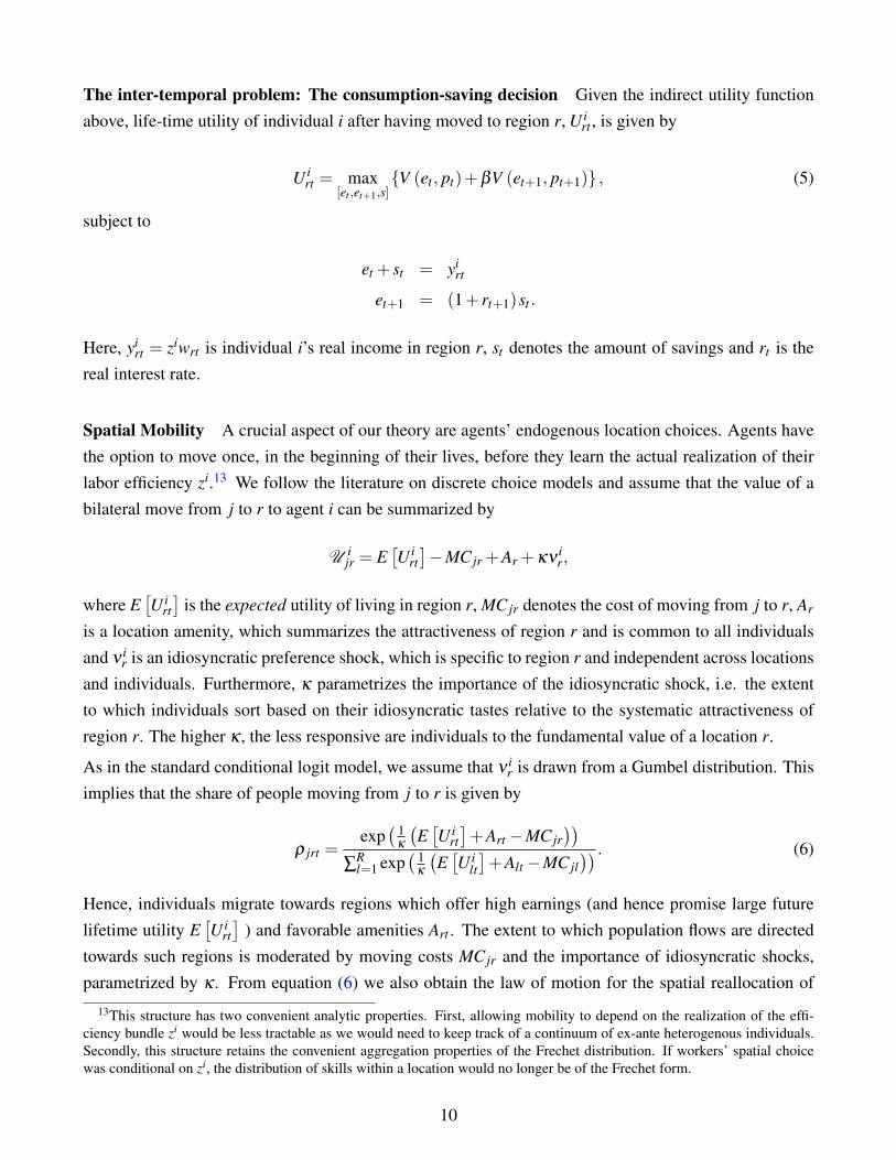
The inter-temporal problem: The consumption-saving decision Given the indirect utility functionabove, life-time utility of individual i after having moved to region r, U i

rt , is given by

U irt = max

[et ,et+1,s]{V (et , pt)+βV (et+1, pt+1)} , (5)

subject to

et + st = yirt

et+1 = (1+ rt+1)st .

Here, yirt = ziwrt is individual i’s real income in region r, st denotes the amount of savings and rt is the

real interest rate.

Spatial Mobility A crucial aspect of our theory are agents’ endogenous location choices. Agents havethe option to move once, in the beginning of their lives, before they learn the actual realization of theirlabor efficiency zi.13 We follow the literature on discrete choice models and assume that the value of abilateral move from j to r to agent i can be summarized by

U ijr = E

[U i

rt]−MC jr +Ar +κν

ir,

where E[U i

rt]

is the expected utility of living in region r, MC jr denotes the cost of moving from j to r, Ar

is a location amenity, which summarizes the attractiveness of region r and is common to all individualsand ν i

r is an idiosyncratic preference shock, which is specific to region r and independent across locationsand individuals. Furthermore, κ parametrizes the importance of the idiosyncratic shock, i.e. the extentto which individuals sort based on their idiosyncratic tastes relative to the systematic attractiveness ofregion r. The higher κ , the less responsive are individuals to the fundamental value of a location r.

As in the standard conditional logit model, we assume that ν ir is drawn from a Gumbel distribution. This

implies that the share of people moving from j to r is given by

ρ jrt =exp( 1

κ

(E[U i

rt]+Art−MC jr

))∑

Rl=1 exp

( 1κ

(E[U i

lt

]+Alt−MC jl

)) . (6)

Hence, individuals migrate towards regions which offer high earnings (and hence promise large futurelifetime utility E

[U i

rt]

) and favorable amenities Art . The extent to which population flows are directedtowards such regions is moderated by moving costs MC jr and the importance of idiosyncratic shocks,parametrized by κ . From equation (6) we also obtain the law of motion for the spatial reallocation of

13This structure has two convenient analytic properties. First, allowing mobility to depend on the realization of the effi-ciency bundle zi would be less tractable as we would need to keep track of a continuum of ex-ante heterogenous individuals.Secondly, this structure retains the convenient aggregation properties of the Frechet distribution. If workers’ spatial choicewas conditional on zi, the distribution of skills within a location would no longer be of the Frechet form.

10

workers between t and t−1 as

Lrt =R

∑j=1

ρ jrtL jt−1, (7)

i.e. the number of people in region r at time t is given by the total inflows from all other regions (includingitself). Since in the model workers only move once, we will discipline the model with data on lifetime

migration, i.e. the extent to which people live (and work) in a different location from where they wereborn (see Molloy et al. (2011)).

3.2 Competitive Equilibrium

We can now characterize the equilibrium of the economy. We proceed in three steps. First we charac-terize the household problem, i.e. the optimal consumption-saving decision and the spatial choice. Wethen show that the solution to the household problem together with our distributional assumptions onindividuals’ skills delivers an analytic solution for the economy’s aggregate demand system. Finally, weshow that individuals’ migration choices only depend on the distribution of equilibrium wages and noton any other future equilibrium variables. This implies that the dynamic competitive equilibrium of oureconomy has a structure akin to the neoclassical growth model: given the sequence of interest rates {rt}t ,we can solve the entire path of spatial equilibria from static equilibrium conditions alone. The equilib-rium sequence of interest rates can then be calculated from the dynamics of the aggregate capital stock,implied by households’ savings decisions. The model can thus be solved by iteratively computing thesequence of spatial equilibria and finding a fixed point for the path of interest rates.

Individual Behavior

First consider the households’ consumption-saving decision given in equation (5). Let the optimal levelof expenditure when young (old) of the generation that is born at time t be denoted by eY

t(eO

t+1). This

two-period OLG structure together with the specification of preferences in equation (4) has a tractablesolution for both the optimal allocation of expenditure and the consumers’ total utility Ur. We summarizethis solution in the following Proposition.

Proposition 1. Consider the maximization problem in equation (5) where V (e, p) is given in equation

(4). The solution to this problem is given by

eYt (y) = ψ (rt+1)y (8)

eOt+1 (y) = (1+ rt+1)(1−ψ (rt+1))y (9)

U irt =Ut (y) =

1η

ψ (rt+1)η−1 yη +Λt,t+1

11

where

ψ (rt+1) =(

1+β1

1−η (1+ rt+1)η

1−η

)−1(10)

Λt,t+1 = −ν

γ

((pAt

pNAt

)γ

+β

(pAt+1

pNAt+1

)γ)+(1+β )

(ν

γ− 1

η

).

Proof. See Section B.2 in the Appendix.

Proposition 1 characterizes the solution to the household problem. Two properties are noteworthy. Firstof all, the policy functions for the optimal amount of spending are linear in earnings. This will allow fora tractable aggregation of individuals’ demands. Moreover, they resemble the familiar OLG structure,where the individual consumes a share ψ (rt+1) of his income when young and consumes the remainder(and the accrued interest) when old. Importantly, this share only depends on the interest rate rt+1 and noton relative prices pt or pt+1.14 If η = 0, i.e. if demand is homothetic, we recover the canonical OLGsolution for log utility where the consumption share is simply given by 1/(1+β ).

Secondly, lifetime utility U irt only depends on the location r via individual income yi

rt . This is due toour assumption that trade is frictionless so that the price indices (which determine Λt,t+1) do not varyacross space. Moreover, utility is additively separable in income yrt and current and future prices Pt

and Pt+1 (which determine Λt,t+1). Both of these properties allow for a tractable solution of individuals’spatial choice problem. To see this, note first that we can calculate individuals’ lifetime utility E

[U i

rt]

analytically: because life-time utility is a power function of individual income yir and individual income

is Frechet distributed, we get that E [yη ] = Γη/ζ wη

rt . Together with equation (6), this delivers closed formexpressions for individual migration decisions, which we summarize in the following Proposition.

Proposition 2. Consider the environment above. Define the relative life-time value of location r at time

t, Wrt , by E[U i

rt]+Art = Wrt +Λt,t+1. Then

Wrt =Γη/ζ

ηψ (rt+1)

η−1 wη

rt +Art . (11)

The share of people moving from j to r at time t, ρ jrt , is then given by

ρ jrt =exp( 1

κ

(Wrt−MC jr

))∑

Rl=1 exp

( 1κ

(Wrt−MC jl

)) . (12)

In particular, ρ jrt is fully determined from static equilibrium wages {wrt}r and exogenous amenities and

does not depend on future prices.

14This is due to our assumption that nominal income e is deflated by the same price index as the investment good. This isconvenient and similar to the single-good neoclassical growth model, where the consumption good and the investment gooduse all factors in equal proportions. For our purposes, this ensures that an increase in the price of the investment good, pIt ,makes savings more attractive but at the same reduces the marginal utility of spending.

12

Proposition 2 implies that individuals’ migration decisions are fully captured by Wrt , which is a summarymeasure of regional attractiveness. Note that the cross-sectional variation in Wrt results from differencesin average wages, wrt , and in amenities Art across labor markets. The former is endogenous and dependson the distribution of regional productivity Qrst , the extent of spatial sorting and aggregate demand con-ditions. In particular, the structural transformation will lower relative wages in agricultural areas andhence raise the return to relocate towards non-agricultural areas. In contrast, regional amenities, whiletime-varying, are fully exogenous. This highlights that the spatial reallocation component of the struc-tural transformation is larger, if the correlation of the initial agricultural employment share srAt−1 andfuture wages wrt and amenities Art is negative and the elasticity of moving flows with respect to suchfundamental differences is large, i.e. κ is small.

Importantly, this expression does not feature Λt,t+1, which is constant across locations and hence does notdetermine spatial labor flows. This implies that agents’ spatial choice problem reduces to a static decisionproblem, which depends only on current, not future, equilibrium objects. This allows us to calculate thetransitional dynamics in the model with a realistic geography, i.e. with about 700 regions.

Equilibrium Aggregation and Aggregate Structural Change

The spatial equilibrium of economic activity is shaped by the heterogeneous local incidence of aggregatedemand and supply conditions. Our economy does not admit a representative consumer, since the PIGLpreference specification falls outside of the Gorman class. To see this, consider a set of individuals i∈S ,with spending ei. The demand for agricultural products by this set of consumers is given by

PCAS =

∫i∈S

ϑA (ei, p)eidi =(

φ +ν

(pA

pNA

)γ ∫i∈S

e−η

i ωidi)

ES ,

where ES =∫

i∈S eidi denotes aggregate spending and ωi = ei/ES is the share of spending of individuali. Hence, as long as preferences are non-homothetic, i.e. as long as η > 0, aggregate demand does notonly depend on aggregate spending ES and relative prices, but on the entire distribution of spending {ei}i.Characterizing the aggregate demand function in our economy, which features heterogeneity throughindividuals’ location choices (and hence in the factor prices they face) and the actual realization of theskill vector zi, is therefore in principle non-trivial.

Our model, however, delivers tractable expressions for the economy’s aggregate quantities. This is due tothree properties of our theory. First of all, the distributional assumption on individual skills implies thatindividual income yi is Frechet distributed. Secondly, Proposition 1 showed that individuals’ expenditurepolicy functions are linear in income yi and hence also Frechet distributed. Finally, individual spendingshares ϑA (e, p) are a power function of expenditure and can therefore be calculated explicitly. Thisallows us to solve for the aggregate demand system explicitly as a function of equilibrium wages.

Proposition 3. Let S gr for g = Y,O be the set of young and old consumers in region r respectively. The

13

aggregate expenditure share on agricultural good of the set of consumers S gr is given by

ϑA([ei]i∈S g

r, p)≡

PCAS g

r

ES gr

= φ + ν

(pA

pNA

)γ

E−η

S gr, (13)

where ES gr

is mean spending at time t and given by

ES Yr= ψ (rt+1)Γζ wrt and ES Y

r= (1+ rt)(1−ψ (rt))Γζ wrt−1,

and ν = νΓ ζ

1−η

/Γ1−η

ζis a constant. The share of agriculture in aggregate spending is given by

ϑAt ≡

PCAt +φ ItPYt

= φ + ν

(pA

pNA

)γ ∑Rr=1

(E1−η

S Yr

Lrt +E1−η

S Or

Lrt−1

)PYt

. (14)

Proof. See Section B.3 in the Appendix.

Proposition 3 is an “almost-aggregation” result. Even though the PIGL preferences fall outside of theGorman class, equation (13) shows that the aggregate demand of a given set of consumers resembles thatof a representative consumer with mean spending ES and an adjusted preference parameter ν . Becausethe linearity of individuals’ policy functions allows to express aggregate spending directly as a functionof equilibrium local wages, aggregate sectoral spending is then simply the spatial aggregate over therespective consumer groups and the aggregate value added share of the agricultural sector takes the formin equation (14). Note that ϑ A

t can be directly calculated from current and past wages {wrt ,wrt−1}r andthe spatial allocation of factors {Lrt ,Lrt−1}r. We exploit this “almost-aggregation” property intensely incomputing the model.

Finally, note that these equations highlight the usual demand side forces of the structural transformation:to the extent that η > 0, i.e. preferences are non-homothetic, the agricultural value added share, ϑ A

t willdecline as income rises. Similarly, changes in relative technological progress (and therefore in sectoralprices) will affect agricultural spending as long as γ 6= 0.

Equilibrium Conditions

Two central properties of our model are that (i) individual moving decisions are static and (ii) that oureconomy generates an aggregate demand system as a function of regional wages. This implies that, for agiven path of interest rates {rt}t , we can calculate the equilibrium by simply solving a sequence of staticequilibrium conditions.

Consider first the goods market. The market clearing condition for agricultural products is given by

LrtΓζ wrtsrAt = (1−α)πrAtϑAt PYt . (15)

14

Hence, total agricultural labor earnings in region r are equal to a share 1−α of total agricultural revenuein region r. This in turn is equal to region r’s share in aggregate spending on agricultural goods ϑ A

t PYt ,πrAt . The CES structure of consumers’ preferences implies that these regional trade shares are given by

πrAt =

(prAt

pAt

)1−σ

=

(QrAtwα−1

rt)σ−1

∑Rj=1

(Q jAtwα−1

jt

)σ−1 , (16)

i.e. they neither depend on the identity of the sourcing region, nor on the equilibrium capital rental rateRt or the common component of productivity ZAt . Rather, region r’s agricultural competitiveness onlydepends on its productivity QrAt and the equilibrium price of labor. An analogous expression holds forthe non-agricultural sector.

To characterize the equilibrium, we find it useful to express the sectoral market clearing conditions inequation (15), as

LrtΓζ wrt = (1−α)(

πrAtϑAt +πrAt

(1−ϑ

At

))PYt (17)

srAt

1− srAt=

πrAt

πrNAt

ϑ At

1−ϑ At. (18)

Equation (17) shows that total earnings in region r are a demand-weighted average of regional sectoraltrade shares and hence highlights the urban bias of the structural transformation: a decline of the aggre-gate agricultural spending share ϑ A

t tends to reduce regional earnings in locations who have a comparativeadvantage, in the agricultural sector. Moreover, equation (18) illustrates the spatial co-movement of sec-toral employment shares. Because regional (scaled) agricultural shares srAt/(1− srAt) are proportional tothe aggregate (scaled) agricultural expenditure share ϑ A

t /(1−ϑ At ), a decline in the aggregate spending

share ϑ At tends to reduce agricultural employment shares in all locations.

These equations also highlight how the spatial distribution of economic activity is fully determinedfrom static equilibrium conditions. Note first that GDP is proportional to aggregate labor earnings, i.e.(1−α)PYt = Γζ ∑r Lrtwrt and that the spatial labor supply function is only a function of the spatial dis-tribution of wages. Likewise the agricultural value added share ϑ A

t only depends on the vector of currentand past wages and population. Together these equilibrium conditions fully determine the equilibriumwages and labor allocations across space.

Finally, since the future capital stock is simply given by the savings of the young generation, we get thatcapital accumulates according to

Kt+1 = (1−ψ (rt+1))∑r

Γζ wrtLrt = (1−ψ (rt+1))(1−α)PYt , (19)

i.e. future capital is simply a fraction 1−ψ (rt+1) of aggregate labor earnings. This proportionalitybetween the aggregate capital stock and aggregate GDP is a consequence of the linearity of agents’

15

consumption policy rules. Note that our model retains many features of the baseline neoclassical growthmodel. In particular, for given initial conditions [K0,{Lr,−1}r,{wr−1}r]} and a path of interest rates{rt}t , the equilibrium evolution of wages and people are solutions to the static equilibrium conditionshighlighted above. A dynamic equilibrium then requires the sequence of interest rates, {rt}t , to beconsistent with the evolution of the capital stock implied by equation (19).

Definition 4. Consider the economy described above. Let the initial capital stock K0, the initial spa-

tial allocation of people {Lr,−1}r and the vector of wages {wr,−1}r be given. A dynamic competitive

equilibrium is a set of prices {prst}rst , wages {wrt}rt , capital rental rates {Rt}t , labor and capital alloca-

tions {Lrst ,Krst}rst , consumption and saving decisions {eYrt ,e

Ort ,srt}rt , and demands for regional varieties

{crst}rst such that consumers’ choices {eYrt ,e

Ort ,srt}rt maximize utility, i.e. are given by equations (8)

and (9), the demand for regional varieties follows equation (16), firms’ factor demands maximize firms’

profits, markets clear, the capital stock evolved according to equation (19) and the allocation of people

across space {LYr,t} is consistent with individuals’ migration choices in equation (6).

To see how “space” and the process of structural change interact, it is instructive to consider a specialcase of our model, where space does not play any interesting role. In particular, consider a parametriza-tion, where (i) there are no moving costs

(MC jr = 0

), (ii) spatial productivities are constant (Qrst = Qrs),

(iii) there are no amenity differences (Art = 0) and (iv) individuals have no idiosyncratic preferences forparticular locations (κ → 0). These assumptions imply that equilibrium wages (and individual welfare)are equalized across space at each point in time. In this case, our model reduces to a standard, macroe-conomic model of the structural transformation augmented by a spatial layer. While the macroeconomicaggregates affect the spatial allocations, there is no feedback from space to the macroeconomy.

To see this, we show in Section B.4 in the Appendix that aggregate GDP in this model is given by anaggregate production function

PYt = ZtKαt L1−α ,

where Zt ≡ Γ1−α

ζZφ

AtZ1−φ

NAt and L = ∑r Lrt . Moreover, it can be shown that - given some initial conditionK0 and processes for productivity {ZAt ,ZNAt}t - there exists a unique dynamic equilibrium path of capital{Kt}t . Furthermore, as in the baseline, aggregate macroeconomic model of the structural transformation,this equilibrium path can be characterized independently of the sectoral labor allocation (see e.g. Herren-dorf et al. (2014)). In particular, suppose that the economy is on a balanced growth path where aggregateincome, capital and wages grow at rate g and the interest rate is constant. The agricultural share in valueadded ϑ A

t is then given by

ϑAt = φ + νχ

(ZNAt

ZAt

)γ

w−η

t ,

where χ is a constant, which is a simple function of exogenous parameters. This relative demand systemagain resembles a representative household with PIGL preferences. Finally, sectoral employment sharesare equal to sectoral value added shares, i.e. sAt = ϑ A

t , so that value added per worker is equalized acrosssectors.

16

While its equilibrium path is independent of the spatial microstructure, this model nevertheless has strongimplications for the allocation of labor across space. In particular, equilibrium trade shares are given byπrst = Qσ−1

rs , i.e. are fully exogenous and only depend on regional productivity (see equation (16)).Moreover, equation (17) implies that the size of the local population is a demand-weighted average ofthe constant local sectoral productivities

Lrt = Qσ−1rA ϑ

At +Qσ−1

rNA

(1−ϑ

At

). (20)

Equation (20) concisely summarizes the urban bias of the structural transformation: A decline in thespending share on agricultural goods reduces population in all regions that have a comparative advan-tage in agricultural goods and increases the size of non-agricultural localities.15 Moreover, because thestructural transformation is the only reason for individuals to relocate, regional population growth andthe initial agricultural employment share are predicted to be perfectly negatively correlated.

Importantly, without spatial frictions, the macroeconomic forces of structural change affect the spatialallocation of factors, but all aggregate allocations can be characterized independently of the spatial mi-crostructure. Like the allocation of resources across sectors, space becomes an inconsequential layer thatis determined residually from the macroeconomic dynamics which are akin to the single-sector neoclas-sical growth model. Both the structural transformation across sectors and its spatial implications are ofsecondary interest for our understanding of the process of economic growth. We therefore refer to thisparametrization of our model also as the Quasi-Spaceless Economy.

This separability between the macroeconomic and spatial allocations breaks down if moving costs orregional amenities generate spatial dispersion in the marginal product of labor. In this case, aggregatestructural change and the spatial allocation of factors are jointly determined. In particular, spatial consid-erations also have implications for the sectoral allocation of resources as average products are no longerequalized. Relative value added per worker in agriculture is for example given by

VAAt /LA

tVAt/Lt

=ϑ A

tsAt

=∑r srAt

wrtLrt∑r wrtLrt

∑r srAtLrt

∑rt Lrt

.

Hence, the agricultural sector has low productivity (i.e. the economy suffers from an “agricultural produc-tivity gap” as in Gollin et al. (2014)), whenever the spatial correlation between wages and agriculturalemployment share is negative. And because the structural transformation puts continuous downwardpressure on wages in agricultural areas, value added per worker in the agricultural areas might remainlow despite the large extent of reallocation out of the agricultural sector. In Section 5.2 we will ex-plicitly compare the aggregate implications of our calibrated model of spatial structural change with theQuasi-Spaceless Economy.

15In fact, it is easy to show that sgn(Qσ−1

rAt −Qσ−1rNAt

)= sgn(srAt − sAt). To see this, note that sAt = ϑ A

t and Qσ−1rst = πrst =

srstLrt/ϑ st .

17

3.3 Selection, Human Capital and Labor Supply

So far we assumed that human capital is perfectly substitutable across sectors and that all individualsare ex-ante identical. In preparation for the quantitative exercise, we now extend our model to allowfor imperfect substitutability of efficiency units across industries and for systematic differences in skill-supply.

We add these ingredients for two reasons. First, the extent of skill substitutability across sectors cru-cially determines the costs of the regional transformation. While moving costs are a hurdle for spatialreallocation, an upward sloping relative sectoral supply function within locations makes it costly to real-locate agricultural workers to factories. Second, systematic differences in skills generate spatial sorting.If skilled workers have a comparative advantage in manufacturing jobs, they are more likely to move tolocations which are productive in the manufacturing sector. Such sorting behavior is a strong feature ofthe data.16 Allowing for such skill differences in the theory allows us to explicitly calibrate our model tobe consistent with the spatial distribution of sectoral employment patterns and skill shares.

Our model can easily be extended along these lines. In particular, we assume that individuals draw atwo-dimensional vector of skill-specific efficiency units zi =

(zi

A,ziNA

)and sort across industries based

on their comparative advantage. We also assume that individuals can be of two types - high skilled andlow skilled. Their skill type h ∈ {L,H} determines the distribution of zi. As before, we assume that zi

s

is drawn independently from a Frechet distribution Fhs (z) = e−Ψh

s z−ζ

, where Ψhs parametrizes the average

level of human capital of individuals of skill type h in sector s. Without loss of generality we parametrizeΨh

s as ΨLA = ΨL

NA = 1 , ΨHNA = µq and ΨH

A = q. Here, q measures the absolute advantage of skilledindividuals and µ governs the comparative advantage of skilled workers in the non-agricultural sector.We denote the share of the aggregate labor force that is skilled by λ and assume that it is constant.17 Incontrast, the spatial allocation of human capital, i.e. the share of skilled workers in region r at time t, λrt ,is endogenous and determined by workers’ migration decisions.

Because of the properties of the Frechet distribution, these additional ingredients leave the rest of thetheoretical analysis almost unchanged. As we show in detail in Section B.5 of the Appendix, the key en-dogenous object is no longer the vector of regional wages wrt , but rather average earnings of individualsin skill group h, which are given by

Eh [yir]= Γζ Θ

hr where Θ

hrt =

(Ψ

hAwζ

rAt +ΨhNAwζ

rNAt

)1/ζ

. (21)

While Θhrt , differs across skill-types, it is equalized across sectors within locations and can be directly

calculated from regional wages (wrA,wrNA), which are no longer equalized across industries within lo-cations. Moreover, the regional attractiveness in Proposition 2 is skill-specific and given by W h

rt =

16See Figure 13 in the Appendix17Hence, we abstract from human capital accumulation and simply assume that skills are fully inherited between parents

and children. Our timing assumption therefore implies that individuals know their skill h ∈ {L,H} prior to migrating but notthe realization of their zi.

18

Γη/ζ

ηψ (rt+1)

η−1 (Θh

rt)η

+ Art . Hence, high skilled individuals put a higher relative weight on non-agricultural wages wrNAt and hence consider locations with a strong manufacturing sector particularlyattractive. Finally, the law of motion of the population is now skill-specific and given by Lrtλ

hrt =

∑Rj=1 ρh

jrtλhrt−1L jt−1, where ρh

jrt is given in Proposition 2. The addition of imperfect skill substitutability,while begetting extra notation, leaves the tractability of our framework untouched and it is this version ofthe model that we take to the data.

4 Spatial Structural Change in the US: 1880 - 2000

We now apply this theory to the experience of the United States over the last 120 years. To do so weconstruct a novel panel data set on the regional development of the United States between 1880 and2000. We describe the data in Section 4.1. One of the main features of our data collection effort is thatwe compile measures of average labor earnings at the regional level. In Section 4.2 we use this data toprovide direct empirical evidence on the urban bias of the structural transformation, i.e. that agriculturallabor markets saw their relative earnings decline. Finally, we calibrate the model in Section 4.3. Ourquantitative analysis is contained in Section 5.

4.1 Data

We combine various data sets published by the US Census Bureau. In particular, we use informationfrom the Census of Manufacturing for 1880 and 1910, the Population Census for 1880-2000 and theCounty and City Data Books for 1940-2000. From these sources we construct a panel data set of totalemployment {Lrt}rt , average manufacturing earnings {wrt}rt , and sectoral employment shares {srAt}rt

for all US counties between 1880 and 2000.18 We define the agricultural sector to comprise agriculture,fishing and mining following the 1950 Census Bureau industrial classification system. All remainingemployed workers are assigned to the non-agricultural sector. We construct average manufacturing wagesfrom county level data on total manufacturing payrolls and manufacturing head counts. To estimate themoving cost parameters we exploit information on lifetime mobility as, in the model, individuals moveonce in their lifetime to access their preferred labor market. All censuses between 1880 and 2000 containinformation on the state of residence and the state of birth. Section E in the Online Appendix contains acomprehensive list of all data sources and more details on the construction of the data set.

We aggregate this county-level data to the level of commuting zones, which we take as our definition of

18Twelve states have not obtained statehood in 1880. These are (with the year of their accession in parentheses): NorthDakota (1889), South Dakota (1889), Montana (1889), Washington (1889), Idaho (1890), Wyoming (1890), Utah (1896),Oklahoma (1907), New Mexico (1912), Arizona (1912), Alaska (1959) and Hawaii (1959). We exclude Alaska, Hawaii andWashington D.C. The 1880 Census does report data for counties in all states, even those that had not yet officially obtainedstatehood in 1880, with two exceptions: Oklahoma and Hawaii. We impute 1880 data for Oklahoma’s counties using aprocedure described in Appendix (E).

19

Q4 (Highest)Q3Q2Q1 (Lowest)No data

Agricultural Employment Shares: Quartiles across Commuting Zones 1880

Q4 (Highest)Q3Q2Q1 (Lowest)No data

Population Growth 1880-1910: Quartiles Across Commuting Zones 1880

Notes: The figure shows the agricultural employment shares in 1880 (left panel) and regional population growth between 1880 and 1910 (right panel) acrossUS commuting zones.

Figure 2: Agricultural Specialization and Population Growth in 1880

a regional labor market (see Tolbert and Sizer (1996)).19 We choose commuting zones for two reasons.First, we need stable regional boundaries over time. Second, labor markets should be large enoughsuch that they contain both an agricultural and a non-agricultural sector. Commuting zones partition thecontinental territory of the United States into 712 polygons. For the main calibration of the model weassume that a period is 30 years and hence employ the cross-sections 1880, 1910, 1940, 1970 and 2000.We normalize the size of the total US workforce to unity in each period.

In Figure 2 we depict the geography of the US at the commuting zone level. In the left panel, weshow the regional agricultural employment shares in 1880. While some regions in Northeastern stateslike Massachusetts or New York already had agricultural employment shares of less than 10%, manycommuting zones in the South had more than 75% of their population employed in the agricultural sector.In the right panel, we show local population growth rates between 1880 and 1910. The absence of a strongcorrelation between population growth and agricultural specialization is apparent. In particular, mostpopulation growth is observed in western commuting zones, which - in 1880 - tend to have intermediateagricultural shares. This already suggests that considerations other than the structural transformationwere important for the observed migration patterns. Below we will use our model to measure thesealternative mechanisms.

In addition, we rely heavily on the 1940 edition of the decennial Micro Census by the US Census Bureau.This is the most recent Census which contains individual identifiers for all US counties and it is the firstCensus for which information on earnings and education is available. We use this information to calibratethe spatial distribution of skilled workers.

Finally, we use micro-data on expenditure patterns from the 1930s to estimate consumer preferences.The Consumer Expenditure Survey in 1936 (“Study of Consumer Purchases in the United States, 1935-

19To do so, we construct a crosswalk between counties and 1990 commuting zones for every decade between 1880 and2000. We aggregate the county level data for the various years to commuting zones, employing area weights to allocateworkers wherever counties are split. A detailed description of the construction of the county to commuting zone cross-walkfor 1790-2000 as well as a panel of the populations of US commuting zones for that period is made available on the authors’website (Eckert et al. (2018)).

20

1936”) contains detailed information on individual expenditure and allows us to calculate the expenditureshare of food. We exploit this cross-sectional information on expenditure shares and total expenditureto estimate the extent of non-homotheticities in demand. Our information for the time-series of relativeprices is taken from Alder et al. (2018).

4.2 The Urban Bias of Structural Change: Direct Evidence

The spatial bias of the structural transformation and the extent to which individuals respond to suchchanging demand condition through migration is a central aspect of our analysis. In this section weprovide some direct evidence on this mechanism, without relying on the calibrated model.

The key implication of the spatial bias is a negative relationship between initial agricultural specializationand subsequent economic performance. In particular, if spatial moving costs are important, the process ofstructural change will reduce factor prices relatively more in agricultural areas. To test this relationship,we consider the regression

lnwMrt+1 = δt,State +α lnsrAt +β lnsrAt×∆sAt+1 + γ lnwM

rt +urt+1,

where wMrt denotes average manufacturing earnings in region r at time t (which are directly observed in

the data), δt,State contains year and state fixed effects, lnsrAt is the log agricultural employment share inregion r and ∆sAt+1 denotes the change in the aggregate agricultural employment share between t andt+1. The coefficient α captures the direct effect of agricultural specialization on manufacturing earningsgrowth. The coefficient β captures the urban bias. In particular, we expect β to be positive: the largerthe decline in the agricultural share, the more adversely will regions with a comparative advantage inagriculture be affected.

The results are reported in Table 1. In the first column, for consistency with Figure 2, we focus on thetime period from 1880 to 1910. In this time period, the aggregate agricultural employment share declinedfrom 50% to around 35%. Cross-sectionally, column 1 shows that regions with a higher agriculturalshare in 1880 experienced lower earnings growth in the subsequent 30 years. Column 2 shows thatthis relationship is not confined to the 1880-1910 period, but holds true in the entire sample. In thelast two columns we directly exploit the panel structure of our data, to estimate the coefficient β fromthe interaction between the initial regional agricultural share and the change in aggregate agriculturalshare. Consistent with an urban bias, a faster decline in the aggregate agricultural employment share isparticularly harmful for regions, which have a larger agricultural share. The results in Table 1 highlightwhy the weak correlation between agricultural employment shares and subsequent population outflowsis surprising: the structural transformation does indeed reduce relative wages in agricultural locations.

21

Dep. variable: ln manufacturing earnings1880-1910 Full Sample

lnsrAt1 -0.040∗∗∗ -0.106∗∗∗ -0.087∗∗∗ -0.063∗∗∗

(0.015) (0.006) (0.007) (0.008)lnsrAt1×∆sAt+1 0.243∗∗∗ 0.247∗∗

(0.094) (0.099)lagged ln man earnings 0.118∗∗∗ 0.120∗∗∗ 0.117∗∗∗ 0.154∗∗∗

(0.022) (0.018) (0.018) (0.021)Year FE X X XState FE X X X XState × Year FE XObservations 717 2868 2868 2868R2 0.594 0.983 0.983 0.985

Notes: Robust standard errors in parentheses with ∗∗∗, ∗∗ and ∗ respectively denoting significance at the 1%, 5% and 10% levels. srA,t is the agricultural shareof region r at time t. ∆sAt+1 is the change in aggregate agricultural employment share between t and t +1.

Table 1: The Urban Bias of Structural Change

The quantitative impact is, however, limited. To see this, consider Figure 3, where we depict the cross-sectional correlation between agricultural employment shares in 1880 and average manufacturing earn-ings in 1910. While there is a negative relationship, there is also ample variation in future wages holdingthe agricultural employment share fixed. This residual variation is important for the correlation betweenagricultural employment shares and population outflows. In our theory, individuals care about the sec-toral composition of a location only in as far as it offers higher life-time utility through favorable factorprices. And Figure 3 suggests that the cohort born in rural areas in 1880 did not necessarily have to movetowards non-agricultural places to increase their life-time earnings.

5.5

6

6.5

7

log

Man

ufac

turin

g Ea

rnin

gs 1

910

0 .2 .4 .6 .8 1Agricultural Employment Share 1880

Notes: The figure shows the correlation between the agricultural employment share in 1880 and the log of average manufacturing earnings in 1910. The sizeof the markers indicates the size of commuting zones as measured by their population in 1880.

Figure 3: Agricultural Specialization and Future Earnings

4.3 Calibration

In this section we describe the calibration of our model. First we discuss our calibration strategy. Wethen turn to the fit of our model with respect to both targeted and non-targeted moments.

22

4.3.1 Calibration Strategy

In this section, we outline the general features of our calibration strategy. In Section D in the OnlineAppendix we provide considerably more detail. Even though our parameters are calibrated jointly, weorganize the discussion of our calibration strategy around the structural parameters and the respectivemoments, which are most informative.

The evolution of aggregate productivity: {ZAt ,ZNAt}t We calibrate the model such that aggregate in-come per capita grows at a constant rate and that the capital-output ratio is constant. In Section B.6 in theAppendix, we show that this implies that interest rates are constant and have a closed-form expression.20

We calibrate the time series of aggregate sectoral productivities, {ZAt ,ZNAt}t , to match the evolution ofrelative prices and a GDP growth rate of 2%.

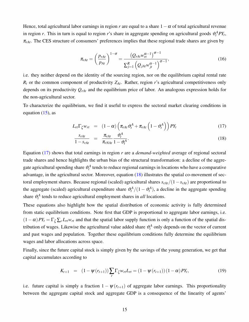
Spatial productivities and amenities: {Qrst ,Art}rst We follow the recent quantitative spatial eco-nomics literature and calibrate local productivities and amenities {Qrst ,Art}rst as structural residuals(Redding and Rossi-Hansberg, 2017). In Appendix D.1 we formally show that there is a unique mappingfrom the observed spatial data on agricultural employment shares, populations and average manufactur-ing earnings to the vector of local productivity {Qrst}rst , conditional on a set of calibrated parameters.Intuitively, local sectoral employment shares contain information on QrAt/QrNAt while the level of wagesalong with the total number of workers informs the level of QrNAt . The vector of amenities {Art}rt canthen be inferred from the observed net population flows.

Moving costs and idiosyncratic location preferences: MC jr and κ We specify the cost of spatialreallocation as having both a fixed and a variable component and we allow the latter to depend on themigration distance in a flexible way. In particular, letting d jr be the distance between j and r, we assumethat

MC jr = τ +δ1d jr +δ2d2jr

whenever j 6= r and zero otherwise. Here, τ > 0 parametrizes the fixed cost of moving and δ1 and δ2

govern how mobility costs vary with distance. We normalize d jr so that the maximum distance in theUS is 1. We calibrate these parameters by matching salient features of the data on lifetime migration.Following Molloy et al. (2011) we measure the aggregate lifetime migration rate as the fraction of peoplewho live in a different location from where they were born.

20Note that ZAt and ZNAt do not grow at a constant rate. Because the reallocation of labor across locations has direct effectson aggregate productivity, a constant rate of GDP growth and a constant interest rate is inconsistent with constant aggregateproductivity growth. See also Herrendorf et al. (2017) for a related discussion. In our counterfactual analysis, interest rateswill of course be free to vary over time.

23

In the Census data we only observe individuals’ region of birth at the state level. We therefore aggre-gate the commuting-zone level migration flows in the model to the level of US states and choose theimportance of locational preferences (κ) and the parameters of mobility costs (τ,δ1,δ2) so as to makethe model best fit the observed state level flows. To capture employment-related mobility, we focus onworkers between 26 and 50 years of age and chose τ so as to match their aggregate lifetime interstate mi-gration rate between 1910 and 1940 exactly. We then chose (κ,δ1,δ2) to minimize the distance betweenspatial mobility rates in the data and the model.21

Preference parameters: η ,γ,φ We estimate the strength of the non-homotheticity in the demand sys-tem (η) from the cross-sectional relationship between sectoral spending shares and the level of expendi-ture. To do so, we use historical micro data from the Consumer Expenditure Survey in 1936, the “Studyof Consumer Purchases in the United States, 1935-1936”. As γ determines the price elasticity of de-mand, we discipline γ with the elasticity of substitution between agricultural and non-agricultural goods.Comin et al. (2017) estimate this elasticity to be around 0.7 in post-war data for the US and we calibrateour model to be consistent with this number. Finally, we use the time-series of the aggregate agriculturalemployment share to identify the remaining parameters φ and ν . Given that our model matches the jointdistribution of agricultural employment shares and population size across space perfectly, internal con-sistency requires us to also match the time series of the aggregate agricultural employment share exactly.The income effects as implied from the cross-sectional spending-food relationship are not strong enoughto explain the entire decline in agricultural employment in the time-series.22 We therefore allow the pa-rameter φ to be time-specific to fully account for the residual decline in agricultural employment andchoose ν to minimize the required time-variation in φt . Intuitively, ν is chosen for the model to explainas much of the aggregate process of structural change as possible, given the income and price elasticitiesη and γ . Recall that φ does not enter the household’s decision problem directly.

Skill supply: ζ ,µ,q and {λr1880}r To parametrize the skill supply, we need values for the supplyelasticity (ζ ), the comparative and absolute advantage of skilled workers (q and µ) and the initial dis-tribution of skilled workers across space in 1880, {λr1880}r. We define skilled individuals as workerswho completed at least high school in 1940 and hold the aggregate share of skilled workers fixed.23 Thischoice yields an aggregate skilled employment share of about 0.3. We then calibrate {λr1880}r for the

21More specifically, we chose (κ,δ1,δ2) to minimize ∑i ∑ j 6=i L j,1940

(logρDATA

i j,1940− logρMODELi j,1940 (κ,δ1,δ2)

)2conditional on

always exactly matching the aggregate interstate migration rate through the choice of τ . As shown in Section D.6 in theAppendix, the number of stayers in a commuting zone is a monotone function in τ given (κ,δ1,δ2).

22This discrepancy between the cross-section and time-series is not particular to our application. For example, the resultsreported in Comin et al. (2017) also imply different estimates for the income elasticity stemming from the cross-section andthe time-series. While reconciling this discrepancy between the cross-section and the time-series is an important open researchquestion, it is not the main focus of our paper.

23Because we focus on the spatial aspects of the structural transformation, we abstract from skill deepening. The modelcould easily be extended to allow for changes in the aggregate supply of human capital.

24

model to exactly replicate the spatial skill distribution in 1940, which is the only year for which edu-cational attainment at the commuting zone level is directly observable. We calibrate the dispersion ofefficiency units ζ , to match the dispersion of earnings in the 1940 Census data. The model implies thatthe variance of log earnings within region-skill cells is given by (π2/6)ζ−2. We therefore identify ζ fromζ = (π/61/2)var

(ui

rsh

)−1/2, where var

(ui

rsh

)is the variance of the estimated residuals from a regression

of log earnings on commuting zone, sector and skill-group fixed effects in the 1940 Census Data.

The two parameters q and µ are chosen to match the aggregate skill premium and the aggregate relativemanufacturing employment share of skilled workers in 1940. We calculate the skill premium as the ratioof average labor earnings of skilled relative to unskilled individuals in the 1940 Census data. Similarly,we compute the relative manufacturing employment share of skilled workers as the non-agriculturalemployment share of skilled workers relative to the one of unskilled workers. Note that these measuresalready incorporate the unbalanced spatial sorting of skilled and unskilled individuals, i.e. they take intoaccount that skilled workers live in high-wage and non-agricultural intensive localities.

Parameter Target Value MomentsData Model

Skill Supplyζ Skill heterogeneity Residual Earnings variance in 1940 1.62 0.62 0.62ξ Share of skilled individuals Share with at least high school in 1940 0.3 0.3 0.3µ Comparative advantage Rel. non-ag. share of skilled workers in 1940 3.41 1.21 1.21q Absolute advantage Skill premium in 1940 0.68 1.62 1.61

[λr1880] Initial distr. of skilled individuals Spatial skill distribution in 1940 . {λr1940} Accounting

Regional Fundamentals[QrAt ]rst Agricultural productivity

Regional empl. shares and earningsSee Appendix

{eManrt ,srAt} Accounting[QrNAt ]rst Non-agricultural productivity

[Art ]rt Amenities Net migration flows {Lhrt}

Time Series Implications[ZNAt ] Non-agricultural productivity Aggregate growth rate of GDP pc See Appendix 2% 2%[ZAt ] Agricultural productivity Relative price of ag. goods See Appendix {pAt/pNAt} Accounting

Preference Parametersβ Discount rate Investment rate along the BGP 0.29 0.15 0.15φ Ag. share in price index Time series of ag. empl. share See Appendix {sAt} {sAt}ν PIGL Preference parameter Time series of ag. empl. share See Appendix {sAt} {sAt}η Non-homotheticity Ag.share - expenditure relationship 0.32 Estimated with NLSγ Price sensitivity Elasticity of substitution in 2000 0.35 0.7 0.7

Moving Costs and Mobilityτ Fixed costs of moving Lifetime interstate migration rate 1.63 0.32 0.32κ Dispersion of idiosyncratic tastes

Observed state-to-state flows0.42 Estimated with NLS

[δ1,δ2] Distance elasticity of moving costs [8.44,−6.39] Estimated with NLSOther parameters

δ Depreciation rate (over 30 years) set exogenously 0.91 (0.08 pa) .α Capital share in production function Aggregate capital share 0.33 . .σ Elasticity of substitution set exogenously 4 . .

Notes: The table contains the calibrated parameters and the main targets. See Section 4.3 for the calibration strategy. In Section D in the Online Appendixwe provide additional details and results.

Table 2: Structural Parameters

25

Other parameters: β ,δ ,σ and α We estimate the rate of time preference β from aggregate macrorelationships. In particular, we chose β to be consistent with the aggregate rate of investment. The capitalshare α is set to match an aggregate capital share of 0.33. The elasticity of substitution between regionalvarieties, σ , is set to 4. In Section 6 below and in the Online Appendix we provide extensive robustnesschecks for this parameter.24 Finally, the depreciation rate δ is set to a 0.08 at annual frequency, which isa central value in the literature.

4.3.2 Calibration Results and Model Fit

In Table 2 we report the calibrated parameters and the main targeted moment, both in the data and themodel. Naturally, the parameters are calibrated jointly.

The presence of spatial mobility costs is an important component of our theory. To see that our modelmatches important features of the lifetime migration data well, we display the distribution of stayersacross states and the relationship between moving flows and distance in Figure 4. In the left panel wedepict the cross-sectional distribution of the share of “stayers”, i.e. ρrr, both in the data and the model.Because regions differ both in attractiveness, i.e. the utility they provide to their residents, and in theirdistance to more attractive places, there is sizable heterogeneity in the extent to which regions are ableto retain workers. Figure 4 shows that the model matches this cross-sectional heterogeneity, even thoughit is only calibrated to match the average rate of mobility. The simple correlation between the share ofstayers in the model and in the data is 0.3. In the right panel, we show that the model also matches thedistance gradient of moving flows. In particular, we run a gravity-type regression of moving flows andcompare the model outcomes to those of the data. We consider the specification

logρ jr

1−ρ j j= α j +βr +u jr,

where α j and βr are origin and destination fixed effects. We then plot the estimated residual u jr asa function of distance for the data and the model. The right panel of Figure 4 shows that the modelcaptures this systematic pattern of lifetime migration flows well. In particular, spatial mobility is verylocal, i.e. spatial flows are steeply decreasing in distance.25

24Allen and Arkolakis (2014) use σ = 9 for a model calibrated to US counties, while Monte et al. (2015) use σ = 4 for thesame purpose. Since we calibrate our model to the more aggregated commuting zones, σ would be expected to be lower. Weconsider values for σ ∈ [3,9].

25The increase in moving flows at large distances stems from the fact that there are sizable coast-to-coast flows.

26

Data Model

.5

1

1.5

2

2.5

.2 .4 .6 .8 1Fraction of Stayers 1910-1940 (States)

Model

Data

-1.5

-.5

.5

1.5

2.5

Log

Inte

rsta

te F

low

s

0 .2 .4 .6 .8 1Normalized Distance

Notes: In the left panel we plot the distribution of the share of people staying in their home state between 1910 and 1940 in the data (grey dotted line) andmodel (orange solid line). To construct the right panel, we run a gravity equation of the form log

(ρ jr/

(1−ρ jr

))= α j +βr + u jr , where ρ jr denotes the

share of people moving from j to r and α j and βr denote origin and destination fixed effects. We run the regression both in the model (orange dots) and inthe data (grey diamonds) and then plot the average u jr by distance percentile.

Figure 4: Lifetime State-to-State Migration: Model vs Data

Bivariate correlationsρ(lnQrNAt , lnQrAt) ρ(lnQrNAt ,Art) ρ(lnQrAt ,Art)

0.225 0.492 0.152

Notes: The table reports the cross-sectional correlation between the spatial fundamentals. We report the average of the correlations for the years 1880, 1910,1940, 1970 and 2000.

Table 3: Correlation of Spatial Fundamentals

An integral part of our calibration strategy is that we calibrate the cross-sectional distribution of sectoralproductivities {QrAt ,QrNAt}rt and amenities {Art}rt as structural residuals (Redding and Rossi-Hansberg,2017). In Table 3 we report the cross-sectional bivariate correlations between these fundamentals. Wefind that productive regions have an absolute advantage in both sectors - the cross-sectional correlationbetween lnQrA and lnQrNA is about 0.225. Similarly, the correlation of productivity and amenities isalso positive, in particular for non-agricultural productivity. Hence, productive places are also relativelypleasant places to live. This is in line with recent direct evidence for developing countries by Gollin etal. (2017). In Section B.8 in the Appendix, we provide additional details about these estimates of spatialfundamentals. In particular, we also relate these model-based measures of regional productivity, Qrst ,to direct empirical measures of local productivity growth. More specifically, we use data on changesin regional market access due to the expansion of the railroad network from Donaldson and Hornbeck(2016) and show these to be highly correlated with changes in {QrA,QrNA}r as inferred from our model.See Section B.9 in the Appendix for details.

Our model of consumer preferences does a good job at replicating the non-homothetic structure of con-sumer demand. Recall that the PIGL demand system implies that expenditure shares at the individuallevel are given by ϑA (e, p) = φ + ν

(pApM

)γ

e−η . For φ ≈ 0, this implies that there is a log-linear re-lationship between expenditure shares and total expenditure. In the left panel of Figure 5 we depict thecross-sectional distribution of the expenditure share for food across US households in 1935. It is apparent

27

that there is substantial heterogeneity and that a large fraction of households has food shares exceeding40%. In the right panel we depict the binned scatter plot between (the log of) expenditures and expen-diture shares after taking out a set of regional fixed effects, to control for relative prices. The slope ofthe regression line is exactly the extent of the demand non-homotheticity η . The expenditure share is notonly systematically declining in the level of expenditure but the cross-sectional relationship is essentiallylog-linear, as predicted by the theory. The slope coefficient implies that η = 0.32.26

0

.02

.04

.06

0 .2 .4 .6 .8 1Expenditure Share for Food

-.4

-.2

0

.2

.4

ln F

ood

Shar

e

-1.5 -1 -.5 0 .5 1ln Expenditure

Notes: The figure shows the cross-sectional distribution of the individual expenditures shares on food (left panel) and the bin scattered relationship betweenthe (log) expenditure share on food and (log) total expenditure (right panel). The relationship in the right panel is conditional on a set of location and familysize fixed effects.

Figure 5: Expenditure Shares on Food in 1936

5 Causes and Consequences of Spatial Structural Change

Using our calibrated model we can now turn to the causes and consequences of spatial structural change.In Section 5.1 we discuss why the urban bias of the structural transformation did not cause more outmi-gration from agricultural areas. In Section 5.2 we ask whether the observed patterns of spatial mobilityhad important implications for aggregate productivity and the spatial distribution of welfare.

5.1 Causes: The Urban Bias and the Pattern of Spatial Reallocation

In Section 4.2 we showed that the mechanism of the urban bias has empirical content: the process ofstructural change did reduce relative wages in agriculturally specialized labor markets and hence was asecular force towards spatial reallocation. However, we also showed that agricultural employment sharesand future earnings were only imperfectly correlated. This tends to weaken the link between populationoutflows and agricultural specialization as migrants might move towards agricultural localities in theirsearch for higher wages. This suggests the presence of important offsetting factors counteracting theurban bias of the structural transformation.

26For our estimate, we of course do not impose the restriction that φ = 0 and estimate the demand function using non-linearleast squares. The parameter η is precisely estimated and - depending on the specification - between 0.3 and 0.34.

28

Our model suggests four main margins. At the individual level, moving costs between labor marketsreduce the level of migration and idiosyncratic motives in individual moving decisions weaken the cor-relation between population net flows and regional factor prices. Because agricultural intensive regionshave (on average) low factor prices, both channels reduce the importance of spatial reallocation for theaggregate decline in agricultural employment. At the regional level, both shocks to spatial fundamentals(i.e. productivities and amenities) and a positive correlation between agricultural comparative advantage(QrA/QrNA) and the level of productivity (QrNA) will reduce the correlation between population outflowsand agricultural employment, as they counteract the secular decline of labor demand in agricultural areas.

To understand the relative importance of these channels, we compare the reallocation patterns of thecalibrated model, which naturally features all channels, with the Quasi-Spaceless Model, characterizedin Section 3, where only the urban bias channel is present.27

Spatial Reallocation in the Quasi-Spaceless Model In the Quasi-Spaceless Model, population mo-bility is only generated by the sectoral shift of spending. Hence, while implying the same decline in theaggregate agricultural share as our baseline model, this model has strikingly different implications forthe link between initial agricultural employment shares and subsequent population flows. In Figure 6 wedepict the share of commuting zones experiencing population outflows between 1910 and 1940 withindifferent deciles of their agricultural employment share in 1910. While the data shows a negative correla-tion between outflows and initial agricultural specialization, the relationship is noisy: even among the setof the regions with the lowest agricultural employment shares in 1910, about 50% experience net popu-lation outflows.28 This is very different for the Quasi-Spaceless Model, where agricultural specializationand population outflows are perfectly aligned. In particular, this model implies that the only regionsexperiencing population inflows are the roughly 17% of commuting zones with the lowest agriculturalshare in 1910.29 Hence, if only the urban bias had been at play, the structural transformation would haveinduced much more population growth in non-agricultural, urban localities.

As a result, the spatial reallocation of individuals explains about one third of the aggregate decline in agri-cultural employment. This is seen in the left panel in Figure 7. Conversely, while the Quasi-SpacelessModel overestimates the role of spatial reallocation, it underestimates the extent of the structural trans-formation at the local level. In particular, in this counterfactual economy, there are more regions whichremain dominated by the agricultural sector throughout the 20th century. Consider, for example, the twored densities on the far left, which corresponds to the year 1970. In the data (the dashed line), the vastmajority of commuting zones have an agricultural employment share below 20%. In the Quasi-Spaceless

27Recall that this model was characterized by the absence of spatial frictions (i.e. MC jr = κ = Ar = 0) and no changes inspatial fundamentals (Qrst = Qrs1880). In practice we set κ to a very small positive number for computational reasons.

28Note that Figure 6 reports the share of regions with net outflows, i.e. the extensive margin of population flows. In theaggregate, net population flows are by construction zero.

29Note that this strong form of sorting is implied by (20): only counties with srAt < sAt see their population increase. Andbecause population size and agricultural employment shares are strongly negatively correlated, far less than half of the regionsare predicted to experience population inflows.

29

0

.2

.4

.6

.8

1

Shar

e of

Reg

ions

w/ N

et O

uflow

s: 1

910-

40

1 2 3 4 5 6 7 8 9 10Agricultural Employment Share Deciles: 1910 (1: Least Agricultural)

Data Quasi-Spaceless Economy

Notes: The figure reports the share of regions within different deciles of the agricultural employment share in 1910, which experience net population outflowsbetween 1910 and 1940. The first (last) decile refers the commuting zones with lowest (highest) agricultural employment share. We report the results for thedata (dark grey) and the Quasi-Spaceless Model, which has no moving costs

(MC jr = 0

), no changes in regional fundamentals (Qrst = Qrs1880), no amenities

(Art = 0) and no idiosyncratic preferences for particular locations (κ → 0).

Figure 6: Agricultural Specialization and Population Outflows

Model, there is a substantial number of regions, where 30%-40% of the workforce are still employedin the agricultural sector. The reason is that worker mobility and the local structural transformation aresubstitutes - the easier it is to reallocate people across space, the more regional specialization can besustained throughout the structural transformation.

We summarize these differences between the Quasi-Spaceless Model and our baseline calibration in thefirst two rows in Table 4. As seen in Figure 7, the spatial reallocation component is equal to 15% andhence five times as large as in the data. Importantly, the net reallocation rate across labor markets isnot substantially different. If only the urban bias channel had been at play, the net migration rate wouldhave been 14%, which is almost identical to the one observed in the data. Hence, in principle, the levelof net spatial reallocation seen in the US was sufficient to account for a large share of the aggregatedecline in agricultural employment. This suggests that the presence of moving frictions cannot be themain counteracting force of the urban bias channel in the data; this is exactly what we find quantitativelyin the next subsection.

Offsetting Factors To better understand which aspect of our theory was the most important to coun-teract the force of the urban bias, we now provide a formal, model-based decomposition of the partialeffects of regional productivity shocks, moving frictions and regional amenities. Because these ingredi-ents interact non-linearly, we quantify the partial effects by calculating both the consequences of addingthe respective ingredient to the Quasi-Spaceless Model and of removing it from our baseline model. Theresults are contained in the lower part of Table 4.

Rows 3 and 4 show that the evolution of spatial productivity was the main reason for the low correlationbetween agricultural specialization and population outflows. If we augment the Quasi-Spaceless Model

30

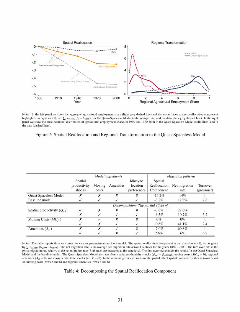
Data

Quasi-Spaceless

Decline in Ag. Empl. Share

Reallocation Component

Data=Quasi-Spaceless-.5

-.3

-.1

0

-.2

-.4

-.61880 1910 1940 1970 2000

Year

Spatial Reallocation

1970 1880

DataQuasi-Spaceless

0

2

4

6

8

0 .2 .4 .6 .8 1Regional Agricultural Employment Share

Regional Transformation

Notes: In the left panel we show the aggregate agricultural employment share (light grey dashed line) and the across labor market reallocation componenthighlighted in equation (1), i.e. ∑r srA1880 (lrt − lr1880), for the Quasi-Spaceless Model (solid orange line) and the data (dark grey dashed line). In the rightpanel we show the cross-sectional distribution of agricultural employment shares in 1910 and 1970, both in the Quasi-Spaceless Model (solid lines) and inthe data (dashed lines).

Figure 7: Spatial Reallocation and Regional Transformation in the Quasi-Spaceless Model

Model ingredients Migration patternsSpatial Idiosync. Spatial

productivity Moving Amenities location Reallocation Net migration Turnovershocks costs preferences Component rate (gross/net)

Quasi-Spaceless Model 7 7 7 7 -15.2% 14% 1Baseline model X X X X -3.2% 12.9% 2.8

Decomposition: The partial effect of ...Spatial productivity (Qrst) X 7 7 7 -3.6% 22.0% 1

7 X X X -6.5% 10.7% 3.2Moving Costs (MC jr) 7 X 7 7 0% 0% 1

X 7 X X -0.6% 41.1% 2.4Amenities (Art) 7 7 X 7 -7.0% 60.8% 1

X X 7 X 2.6% 6% 6.2

Notes: The table reports three outcomes for various parametrization of our model. The spatial reallocation component is calculated as in (1), i.e. is givenby ∑r srA1880 (lr2000− lr1880). The net migration rate is the average net migration rate across US states for the years 1880 - 2000. The turn over rate is thegross migration rate relative to the net migration rate. Both rates are measured at the state level. The first two rows contain the results for the Quasi-SpacelessModel and the baseline model. The Quasi-Spaceless Model abstracts from spatial productivity shocks (Qrst = Qrs1880), moving costs

(MC jr = 0

), regional

amenities (Art = 0) and idiosyncratic taste shocks (i.e. κ → 0). In the remaining rows we measure the partial effect spatial productivity shocks (rows 3 and4), moving costs (rows 5 and 6) and regional amenities (rows 7 and 8).

Table 4: Decomposing the Spatial Reallocation Component

31

with the observed process of spatial productivity, the implied spatial reallocation component would be-3.6%. This is almost exactly the same number as observed in the data. Similarly, if we start from thebaseline model but abstract from regional productivity changes, the impact of spatial reallocation wouldhave doubled from 3.2% to 6.5%. The reason is that regional productivity shocks introduce noise inthe relationship between earnings growth and initial agricultural specialization and hence weaken thequantitative importance of the urban bias.

In contrast, moving costs and regional amenities play less of a role. While adding moving costs to theQuasi-Spaceless Model does reduce the role of spatial reallocation, it does so for the wrong reason: theimplied level of migration is essentially zero. More interestingly, row 6 shows that without moving costsour baseline model would predict the spatial reallocation component to be even lower - 0.6% comparedto -3.2% in the data. The reason is that a reduction in moving costs would not only induce people tomove towards regions with high earnings but also trigger more mobility for idiosyncratic reasons. Thelatter moves are by construction uncorrelated with agricultural specialization and hence do not contributeto the spatial reallocation component of structural change. Similarly, regional amenities cannot explainthe quasi-absence of the spatial reallocation component in the data. In fact, the last row of Table 4 showsthat the role of spatial reallocation would have been even smaller in the absence of amenities. If anything,the correlation between agricultural shares and population growth had been positive! Since rural regionshave (on average) low future amenities (see Table 3), the amenity channel provides an additional pushfactor out of agricultural labor markets. This is consistent with the direct empirical evidence reported inGollin et al. (2017) for developing countries today.

One final important difference between our baseline model and the Quasi-Spaceless Model is the exis-tence of idiosyncratic preference shocks for particular locations. The reason why our model infers thatidiosyncratic shocks are empirically important is the prevalence of bi-directional flows in the data. Ifidiosyncratic shocks were absent, all individuals would agree on the ranking of potential destinations andthe gross and net flows between any pair of locations would coincide. The “turnover” rate, i.e. the ratioof the gross and net migration rate, is therefore a measure of the importance of idiosyncratic migrationmotives. It can be interpreted as the number of bodies that have to be moved across space to reallocateone person “on net” between regions. The last column of Table 4 shows that the turnover rate in the dataand in our baseline model is around 3. This is in sharp contrast to the Quasi-Spaceless Model, where thisratio is 1, as gross and net flows coincide.30

5.2 Consequences: Aggregate Productivity and Spatial Welfare

We now turn to the macroeconomic implications of spatial structural change. We focus on two aggregateoutcomes: aggregate productivity and the spatial distribution of welfare. The urban bias of the struc-

30To be precise, in the absence of moving costs, the equilibrium allocation of net flows is unique, but the gross flows arenot determined. This indeterminacy vanishes for an arbitrarily small moving cost. In that case, the net migration rate is equalto the gross migration rate.

32

Baseline Model CounterfactualsQuasi-Spaceless Model No Spatial Mobility

Decline in Agricultural Employment Share -48.1% -48% -47.8%Net migration rate 13% 14% 0Spatial Reallocation Component -3.2% -15.2% 0

Aggregate ProductivityIncrease in GDP pc (rel. to 1880) 10.78 11.04 8.89

Difference to baseline 2.4% -17.5%Agricultural productivity Gap 0.83 0.79 0.73

Spatial Welfare InequalityLow Skilled Workers 1910 157% 0 202%

∆ 1910 - 2000 -35% - -13%High Skilled Workers 1910 149% 0 205%

∆ 1910 - 2000 -38% - -24%

Notes: The model with no spatial mobility corresponds to the baseline model except that individuals are not allowed to move (i.e. MC jr → ∞). The Quasi-Spaceless Model assumes that moving costs are zero (i.e. MC jr = 0), that there are no amenities (Art = 0) and no idiosyncratic tastes (i.e. κ = 0) and thatregional technologies are constant, i.e. Qrst = Qrs1880. The net migration rate is the average migration rate between 1910 and 2000. The spatial reallocationcomponent is calculated as in (1), i.e. is given by ∑r srA1880 (lr2000− lr1880). The “Agricultural Productivity Gap” is measured as aggregate value addedper worker in agriculture relative the rest of the economy, i.e.

(VAA

t /LAt)/(VAt/Lt), in the year 2000. For the calculation of the spatial welfare inequality

measure we refer to the main text.

Table 5: Aggregate Implications of Spatial Structural Change

tural transformation systematically changes the marginal product of labor across labor markets. If andhow fast workers reallocate spatially therefore has important implications for allocative efficiency andhence aggregate productivity of the US economy. Furthermore, in the presence of spatial frictions, thissecular demand shift also has distributional consequence by lowering relative wages in agricultural re-gions. Labor mobility therefore tends to both increase allocative efficiency and reduce spatial inequality.To quantify these consequences of spatial structural change, we therefore compare our model with theQuasi-Spaceless Economy, where space and the structural transformation do not interact. For comparisonwe also consider a model without any labor mobility by making the costs of moving prohibitively high.

Spatial Structural Change and Aggregate Productivity We report the outcomes of these three differ-ent models in Table 5. In the first row, we verify that all models generate a similar decline in the aggregateagricultural share. Hence, the aggregate “size” of the structural transformation is constant across specifi-cations. For convenience we again report the average amount of spatial reallocation (as measured by thenet migration rate) and the spatial reallocation component of the structural transformation in rows 2 and3.

In the lower panel, we report the implications for aggregate GDP growth. If spatial mobility had beenonly based on regional earnings and mobility was free, income per capita would have been roughly 2.5%higher. Hence, the local nature of the structural transformation did interfere with allocative efficiency.Nevertheless, quantitatively, these efficiency gains seem modest.31 This, however, does not imply that

31To put these results into perspective, Bryan and Morten (2017), using a static spatial equilibrium model, estimate higher

33

migration was unimportant for the US economy during the structural transformation.32 Without labormobility, income per capita would have been lower by almost 17.5%. Hence, spatial mobility contributedheavily to aggregate productivity growth during the transition away from agriculture.

These differences in allocative efficiency are also reflected in sectoral productivity gaps. Both the base-line model and the model without spatial frictions, for example, imply an agricultural productivity gapof around 20% even though there are no sectoral frictions. These productivity differences are to a largeextent due to skill-based sorting, whereby high-skilled individuals both work in the non-agricultural sec-tor within regions and move towards urban locations spatially. Without spatial mobility this gap wouldincrease to 27% as the structural transformation amplifies wage differences between agricultural andnon-agricultural regions and workers sort less effectively.

The Distributional Effects of Spatial Structural Change We now turn to the evolution of spatialwelfare inequality. As in Proposition 2 we focus on the expected life-time value of being in location r,W h

rt = Eh [Ur] +Art , as our measure of regional welfare for skill group h. Our model implies that bothregional income Θh

r and regional amenities are negatively correlated with the agricultural employmentshare so that welfare is systematically lower in agriculturally intensive places. Moreover, the spatialbias of the structural transformation is an additional inequality-enhancing force. At the same time, labormobility tends to keep wage disparities in check and changing regional productivities are inequality-reducing as they show mean-reversion.

To quantify the evolution of spatial welfare inequality during the 20th century, we convert utility differ-ences into “life-time-income” equivalents. Specifically, let ∆h

t denote the interquartile range of W hrt at

time t. Let T hrt be the increase of expected lifetime income, an individual with skill h in region r requires

to increase utility of living in region r by ∆ht , i.e. W h

rt(T h

rt y)≡ W h

rt (y) +∆ht . Our measure of spatial

inequality for individuals of skill h is then given as the cross-regional average of T hrt , i.e. T h

t = 1R ∑T h

rt .

We report the results in the lower panel of Table 5. Spatial welfare inequality decreased substantiallyduring the structural transformation. In 1910, low skilled workers in the average region would haverequired an increase in average lifetime income by about 160% to increase utility by the interquartilerange of regional welfare differences. In 2000, lifetime income would only have to be doubled. Hence,the dispersion in spatial welfare declined by about 35% since 1910. The corresponding numbers for highskilled individuals are quantitatively quite similar.33

productivity losses from limited labor mobility for Indonesia. In their specifications without agglomeration and endogenousamenities, which we for simplicity abstract from in our model, they find that productivity would increase by about 17% ifmoving costs were zero and there were no amenity differences. There are two main reasons, why our results are small. Firstof all, by explicitly considering capital as a factor of production (which can be traded without frictions) our economy allowsfor some factor other than labor to adjust. Secondly, Bryan and Morten (2017) argue that the US economy has lower mobilitycosts than Indonesia. If we recalibrate our model under the assumption that α = 0.05, i.e. that labor is (essentially) the solefactor of production, we find that relative GDP the Quasi-Spaceless Model is 13% higher. This is comparable to the resultsreported in Bryan and Morten (2017).

32Note that agricultural productivity gap is slightly higher in the Quasi-Spaceless Model. The reason is that model impliesmore spatial sorting of skilled workers.

33The decline in inequality is not driven by changes in the distribution of regional amenities. The dispersion in amenities is

34

Spatial mobility was a crucial factor for this decline in welfare inequality. Without any spatial frictions,welfare would obviously be equalized at each point in time. This is the case in the Quasi-SpacelessEconomy. Conversely, without any spatial mobility since 1880, both the level of welfare inequalitywould have been higher and the decline would have been much smaller. This margin was a particularlyimportant adjustment mechanism for low-skilled workers as these workers have a comparative advantagein the agricultural sector and hence are particularly exposed to the the structural transformation. Spa-tial mobility was therefore a crucial adjustment mechanism for low-skilled workers to weather the firststructural transformation away from agriculture. Without it, spatial welfare inequality would have beensubstantially higher.

6 Robustness

In this section we demonstrate the robustness of our results to a range of alternative parametrizations ofthe model. We focus on the spatial reallocation component of the structural transformation (Table 4) andthe effects of spatial mobility on aggregate GDP (Table 5). In Section D.8 of the Online Appendix weprovide more details.

The results are summarized in Table 6. For the spatial reallocation components we again report theimplications of the Quasi-Spaceless Economy and the decomposition into the individual margins byremoving the respective ingredient from our baseline calibration. For the implications for aggregate GDP,we report the change of GDP in 2000 for the economy without mobility and the frictionless economyrelative to the baseline. For all specifications, we always recalibrate the spatial structural residuals andaggregate technology series.34 Hence, the spatial reallocation component and the evolution of GDP isidentical across specifications.

roughly constant between 1910 and 2000 and spatial welfare differences had declined even in the absence of amenities.34Specifically, we always match the time series data on relative prices and aggregate GDP and the spatial data on earnings,

population size and agricultural employment shares.

35

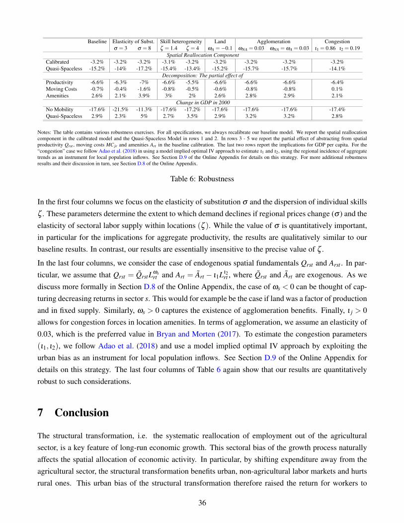
Baseline Elasticity of Subst. Skill heterogeneity Land Agglomeration Congestionσ = 3 σ = 8 ζ = 1.4 ζ = 4 ωA =−0.1 ωNA = 0.03 ωNA = ωA = 0.03 ι1 = 0.86 ι2 = 0.19

Spatial Reallocation ComponentCalibrated -3.2% -3.2% -3.2% -3.1% -3.2% -3.2% -3.2% -3.2% -3.2%Quasi-Spaceless -15.2% -14% -17.2% -15.4% -13.4% -15.2% -15.7% -15.7% -14.1%

Decomposition: The partial effect ofProductivity -6.6% -6.3% -7% -6.6% -5.5% -6.6% -6.6% -6.6% -6.4%Moving Costs -0.7% -0.4% -1.6% -0.8% -0.5% -0.6% -0.8% -0.8% 0.1%Amenities 2.6% 2.1% 3.9% 3% 2% 2.6% 2.8% 2.9% 2.1%

Change in GDP in 2000No Mobility -17.6% -21.5% -11.3% -17.6% -17.2% -17.6% -17.6% -17.6% -17.4%Quasi-Spaceless 2.9% 2.3% 5% 2.7% 3.5% 2.9% 3.2% 3.2% 2.8%

Notes: The table contains various robustness exercises. For all specifications, we always recalibrate our baseline model. We report the spatial reallocationcomponent in the calibrated model and the Quasi-Spaceless Model in rows 1 and 2. In rows 3 - 5 we report the partial effect of abstracting from spatialproductivity Qrst , moving costs MC jr and amenities Art in the baseline calibration. The last two rows report the implications for GDP per capita. For the“congestion” case we follow Adao et al. (2018) in using a model implied optimal IV approach to estimate ι1 and ι2, using the regional incidence of aggregatetrends as an instrument for local population inflows. See Section D.9 of the Online Appendix for details on this strategy. For more additional robustnessresults and their discussion in turn, see Section D.8 of the Online Appendix.

Table 6: Robustness

In the first four columns we focus on the elasticity of substitution σ and the dispersion of individual skillsζ . These parameters determine the extent to which demand declines if regional prices change (σ ) and theelasticity of sectoral labor supply within locations (ζ ). While the value of σ is quantitatively important,in particular for the implications for aggregate productivity, the results are qualitatively similar to ourbaseline results. In contrast, our results are essentially insensitive to the precise value of ζ .

In the last four columns, we consider the case of endogenous spatial fundamentals Qrst and Arst . In par-ticular, we assume that Qrst = QrstL

ωsrt and Art = Art − ι1Lι2

rt , where Qrst and Art are exogenous. As wediscuss more formally in Section D.8 of the Online Appendix, the case of ωs < 0 can be thought of cap-turing decreasing returns in sector s. This would for example be the case if land was a factor of productionand in fixed supply. Similarly, ωs > 0 captures the existence of agglomeration benefits. Finally, ι j > 0allows for congestion forces in location amenities. In terms of agglomeration, we assume an elasticity of0.03, which is the preferred value in Bryan and Morten (2017). To estimate the congestion parameters(ι1, ι2), we follow Adao et al. (2018) and use a model implied optimal IV approach by exploiting theurban bias as an instrument for local population inflows. See Section D.9 of the Online Appendix fordetails on this strategy. The last four columns of Table 6 again show that our results are quantitativelyrobust to such considerations.

7 Conclusion

The structural transformation, i.e. the systematic reallocation of employment out of the agriculturalsector, is a key feature of long-run economic growth. This sectoral bias of the growth process naturallyaffects the spatial allocation of economic activity. In particular, by shifting expenditure away from theagricultural sector, the structural transformation benefits urban, non-agricultural labor markets and hurtsrural ones. This urban bias of the structural transformation therefore raised the return for workers to

36

relocate spatially. In this paper, we use a novel theory of spatial structural change and detailed regionaldata to analyze the spatial nature of the structural transformation in the US between 1880 and 2000.

We first document empirically that the spatial reallocation of workers towards non-agricultural labormarkets explained essentially none of the decline in the aggregate agricultural employment share from50% to nearly zero over the last 120 years. In contrast, the entire decline is accounted for by within labormarket changes, whereby agricultural employment declined in each locality. While these patterns seemto contradict the large increase in urbanization over the same time-period, we show that this is not thecase: like the change in agricultural employment, the increase in the share of urban dwellers was alsovery local in nature.

To explain this fact and to understand whether this mode of adjustment had important aggregate impli-cations, we construct a new quantitative theory of the structural transformation that explicitly incorpo-rates a spatial layer. The model combines the basic features of an economic geography model featuringcostly labor mobility with the canonical ingredients of neoclassical models of structural change, i.e. non-homothetic preferences, unbalanced technological progress and aggregate capital accumulation. Despitethis richness, we show that the analysis remains highly tractable and can be applied to a realistic geogra-phy.

Our analysis yields two main results. First, we show that the evolution of spatial productivity was themain reason for the insignificance of the spatial reallocation channel. Because local productivity is sub-ject to shocks and regional absolute and comparative advantage are imperfectly correlated, the relation-ship between agricultural specialization and future earnings (and hence net population outflows) is onlyweakly negative - despite the urban bias of the structural transformation. Secondly, we show that thepossibility of spatial reallocation had important macroeconomic consequences. First, the process of spa-tial arbitrage was an important contributor of aggregate productivity growth in the US. Without labormobility, aggregate income would have been 17% smaller. Additionally, it played a crucial role for theevolution of spatial welfare inequality during the structural transformation of the US. In the absence ofmigration across labor markets, welfare inequality would have been markedly higher, in particular amongunskilled workers, which were especially exposed to the secular demand shift away from agriculture.

References

Acemoglu, Daron and Veronica Guerrieri, “Capital Deepening and Nonbalanced Economic Growth,”Journal of Political Economy, 2008, 116 (3), 467–498.

Adao, Rodrigo, Costas Arkolakis, and Federico Esposito, “Trade, Agglomeration Effects, and LaborMarkets: Theory and Evidence,” 2018.

Ahlfeldt, Gabriel M., Stephen J. Redding, Daniel M. Sturm, and Nikolaus Wolf, “The Economics ofDensity: Evidence From the Berlin Wall,” Econometrica, 2015, 83 (6), 2127–2189.

37

Alder, Simon, Timo Boppart, and Andreas Muller, “A Theory of Structural Change that Can Fit theData,” 2018.

Allen, Treb and Costas Arkolakis, “Trade and the Topography of the Spatial Economy,” The Quarterly

Journal of Economics, 2014, 129 (3), 1085–1140.

Alvarez-Cuadrado, Francisco and Markus Poschke, “Structural Change out of Agriculture: LaborPush versus Labor Pull,” American Economic Journal: Macroeconomics, 2011, 3 (3), 127–158.

, Ngo Van Long, and Markus Poschke, “Capital Labor Substitution, Structural Change, and Growth,”Theoretical Economics, 2017, 12 (3), 1229–1266.

Baumol, William J, “Macroeconomics of Unbalanced Growth: the Anatomy of Urban Crisis,” American

Economic Review, 1967, 57 (3), 415–426.

Boppart, Timo, “Structural Change and the Kaldor Facts in a Growth Model With Relative Price Effectsand Non-Gorman Preferences,” Econometrica, 2014, 82 (6), 2167–2196.

Bryan, Gharad and Melanie Morten, “The Aggregate Productivity Effects of Internal Migration: Evi-dence from Indonesia,” 2017.

, Shyamal Chowdhury, and Ahmed Mushfiq Mobarak, “Underinvestment in a Profitable Technol-ogy: The Case of Seasonal Migration in Bangladesh,” Econometrica, 2014, 82 (5), 1671–1748.

Buera, Francisco J and Joseph P Kaboski, “Can Traditional Theories of Sructural Change Fit theData?,” Journal of the European Economic Association, 2009, 7 (2-3), 469–477.

Caselli, Francesco and Wilbur John Coleman II, “The U.S. Structural Transformation and RegionalConvergence: A Reinterpretation,” Journal of Political Economy, 2001, 109 (3), 584–616.

Chenery, Hollis B, “Patterns of Industrial Growth,” American Economic Review, 1960, 50 (4), 624–654.

Comin, Diego, Danial Lashkari, and Martı Mestieri, “Structural Change with Long-Run Income andPrice Effects,” 2017.

Desmet, Klaus and Esteban Rossi-Hansberg, “Spatial Development,” American Economic Review,2014, 104 (4), 1211–43.

Diamond, Rebecca, “The Determinants and Welfare Implications of US Workers’ Diverging LocationChoices by Skill: 1980-2000,” American Economic Review, March 2016, 106 (3), 479–524.

Donaldson, Dave and Richard Hornbeck, “Railroads and American Economic Growth: A MarketAccess Approach,” The Quarterly Journal of Economics, 2016, 131 (2), 799–858.

38

Eckert, Fabian, Andres Gvirtz, and Michael Peters, “Constructing a Population Panel for US Com-muting Zones 1790-2000,” 2018.

Fajgelbaum, Pablo and Stephen J. Redding, “External Integration, Structural Transformation and Eco-nomic Development: Evidence from Argentina 1870-1914,” Working Paper 20217, National Bureauof Economic Research June 2014.

Fajgelbaum, Pablo D., Eduardo Morales, Juan Carlos Suarez Serrato, and Owen M. Zidar, “StateTaxes and Spatial Misallocation,” Working Paper 21760, National Bureau of Economic ResearchNovember 2015.

Gollin, Douglas, David Lagakos, and Michael E. Waugh, “The Agricultural Productivity Gap,” The

Quarterly Journal of Economics, 2014, 129 (2), 939–993.

, Martina Kirchberger, and David Lagakos, “In Search of a Spatial Equilibrium in the DevelopingWorld,” Working Paper 23916, National Bureau of Economic Research October 2017.

, Stephen Parente, and Richard Rogerson, “The Role of Agriculture in Development,” American

Economic Review, May 2002, 92 (2), 160–164.

Herkenhoff, Kyle F, Lee E Ohanian, and Edward C Prescott, “Tarnishing the golden and empirestates: Land-use restrictions and the US economic slowdown,” Journal of Monetary Economics, 2017.

Herrendorf, Berthold and Todd Schoellman, “Why is Measured Productivity so Low in Agriculture?,”Review of Economic Dynamics, 2015, 18 (4), 1003–1022.

, Christopher Herrington, and Akos Valentinyi, “Sectoral Technology and Structural Transforma-tion,” American Economic Journal: Macroeconomics, October 2015, 7 (4), 104–33.

, Richard Rogerson, and Akos Valentinyi, “Two Perspectives on Preferences and Structural Trans-formation,” American Economic Review, December 2013, 103 (7), 2752–89.

, , and , “Chapter 6 - Growth and Structural Transformation,” in Philippe Aghion and Steven N.Durlauf, eds., Handbook of Economic Growth, Vol. 2 of Handbook of Economic Growth, Elsevier,2014, pp. 855 – 941.

, , and , “Structural Change in Investment and Consumption: A Unified Approach,” 2017. Work-ing Paper.

Hobijn, Bart, Todd Schoellman, and Alberto J. Vindas Q., “Structural Transformation:A Race be-tween Demographics and Technology,” 2018. Mimeo, Arizona State University.

Hsieh, Chang-Tai and Enrico Moretti, “Housing Constraints and Spatial Misallocation,” Working Pa-per 21154, National Bureau of Economic Research May 2015.

39

Kongsamut, Piyabha, Sergio Rebelo, and Danyang Xie, “Beyond Balanced Growth,” The Review of

Economic Studies, 2001, 68 (4), 869–882.

Kuznets, Simon, “Quantitative Aspects of the Economic Growth of Nations: II. Industrial Distributionof National Product and Labor Force,” Economic Development and Cultural Change, 1957, pp. 1–111.

Lagakos, David and Michael E. Waugh, “Selection, Agriculture, and Cross-Country Productivity Dif-ferences,” American Economic Review, April 2013, 103 (2), 948–80.

, Mushfiq Mobarak, and Michael E Waugh, “The Welfare Effects of Encouraging Rural-UrbanMigration,” 2017.

Lindbeck, Assar, ed., Nobel Lectures, Economics 1969-1980, World Scientific Publishing Co., Singa-pore, 1992.

Michaels, Guy, Ferdinand Rauch, and Stephen J Redding, “Urbanization and Structural Transforma-tion,” The Quarterly Journal of Economics, 2012, 127 (2), 535–586.

Molloy, Raven, Christopher L. Smith, and Abigail Wozniak, “Internal Migration in the United States,”Journal of Economic Perspectives, September 2011, 25 (3), 173–96.

Monte, Ferdinando, Stephen J. Redding, and Esteban Rossi-Hansberg, “Commuting, Migrationand Local Employment Elasticities,” Working Paper 21706, National Bureau of Economic ResearchNovember 2015.

Nagy, Dávid Krisztián, “City Location and Economic Development,” 2017.

Ngai, L. Rachel and Christopher A. Pissarides, “Structural Change in a Multisector Model of Growth,”American Economic Review, March 2007, 97 (1), 429–443.

Porzio, Tommaso and Gabriella V. Santangelo, “Structural Change and the Supply of AgriculturalWorkers,” 2017.

Redding, Stephen J. and Daniel M. Sturm, “The Costs of Remoteness: Evidence from German Divi-sion and Reunification,” American Economic Review, December 2008, 98 (5), 1766–97.

and Esteban Rossi-Hansberg, “Quantitative Spatial Economics,” Annual Review of Economics,2017, 9 (1), 21–58.

Ruggles, Steven, Matthew Sobek, Trent Alexander, Catherine A Fitch, Ronald Goeken, Patri-cia Kelly Hall, Miriam King, and Chad Ronnander, “Integrated Public Use Microdata Series: Ver-sion 6.0 [dataset]. Minneapolis: University of Minnesota, 2015,” 2015.

Tolbert, Charles M and Molly Sizer, “US commuting zones and labor market areas: A 1990 update,”1996.

40

Tombe, Trevor, Xiaodong Zhu et al., “Trade, Migration and Productivity: A Quantitative Analysis ofChina,” 2015.

Young, Alwyn, “Inequality, the Urban-Rural Gap, and Migration,” The Quarterly Journal of Economics,2013, 128 (4), 1727–1785.

41

APPENDIX

42

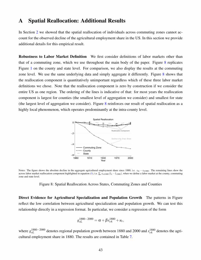
A Spatial Reallocation: Additional Results

In Section 2 we showed that the spatial reallocation of individuals across commuting zones cannot ac-count for the observed decline of the agricultural employment share in the US. In this section we provideadditional details for this empirical result.

Robustness to Labor Market Definition We first consider definitions of labor markets other thanthat of a commuting zone, which we use throughout the main body of the paper. Figure 8 replicatesFigure 1 on the county and state level. For comparison, we also display the results at the commutingzone level. We use the same underlying data and simply aggregate it differently. Figure 8 shows thatthe reallocation component is quantitatively unimportant regardless which of these three labor marketdefinitions we chose. Note that the reallocation component is zero by construction if we consider theentire US as one region. The ordering of the lines is indicative of that: for most years the reallocationcomponent is largest for counties (the smallest level of aggregation we consider) and smallest for state(the largest level of aggregation we consider). Figure 8 reinforces our result of spatial reallocation as ahighly local phenomenon, which operates predominantly at the intra-county level.

Reallocation Component

Decline in Ag. Empl. Share

0

-.2

-.4

-.61880 1910 1940 1970 2000

Year

Commuting ZoneCountyState

Spatial Reallocation

Notes: The figure shows the absolute decline in the aggregate agricultural employment share since 1880, i.e. sAt − sA1880. The remaining lines show theacross labor market reallocation component highlighted in equation (1), i.e. ∑r srA1880 (lrt − lr1880), when we define a labor market at the county, commutingzone and state level.

Figure 8: Spatial Reallocation Across States, Commuting Zones and Counties

Direct Evidence for Agricultural Specialization and Population Growth The patterns in Figurereflect the low correlation between agricultural specialization and population growth. We can test thisrelationship directly in a regression format. In particular, we consider a regression of the form

g1880−2000rL = α +β s1880

rA +ur,

where g1880−2000rL denotes regional population growth between 1880 and 2000 and s1880

rA denotes the agri-cultural employment share in 1880. The results are contained in Table 7.

43

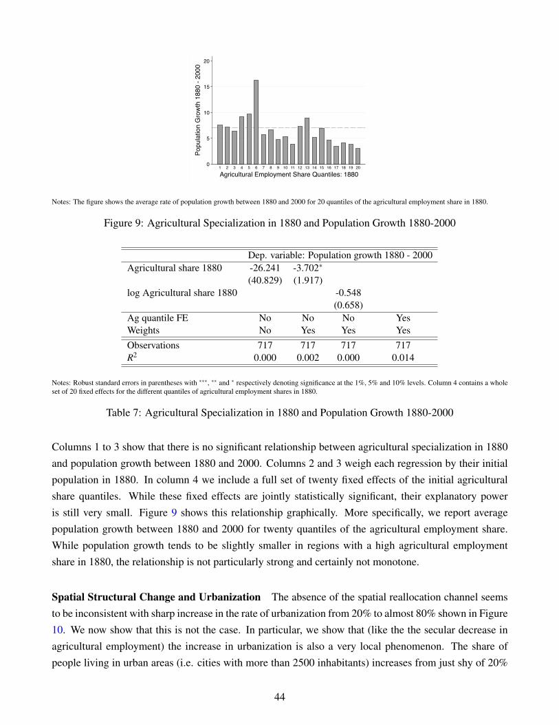
0

5

10

15

20

Popu

latio

n G

row

th 1

880

- 200

0

1 2 3 4 5 6 7 8 9 10 11 12 13 14 15 16 17 18 19 20

Agricultural Employment Share Quantiles: 1880

Notes: The figure shows the average rate of population growth between 1880 and 2000 for 20 quantiles of the agricultural employment share in 1880.

Figure 9: Agricultural Specialization in 1880 and Population Growth 1880-2000

Dep. variable: Population growth 1880 - 2000Agricultural share 1880 -26.241 -3.702∗

(40.829) (1.917)log Agricultural share 1880 -0.548

(0.658)Ag quantile FE No No No YesWeights No Yes Yes YesObservations 717 717 717 717R2 0.000 0.002 0.000 0.014

Notes: Robust standard errors in parentheses with ∗∗∗, ∗∗ and ∗ respectively denoting significance at the 1%, 5% and 10% levels. Column 4 contains a wholeset of 20 fixed effects for the different quantiles of agricultural employment shares in 1880.

Table 7: Agricultural Specialization in 1880 and Population Growth 1880-2000

Columns 1 to 3 show that there is no significant relationship between agricultural specialization in 1880and population growth between 1880 and 2000. Columns 2 and 3 weigh each regression by their initialpopulation in 1880. In column 4 we include a full set of twenty fixed effects of the initial agriculturalshare quantiles. While these fixed effects are jointly statistically significant, their explanatory poweris still very small. Figure 9 shows this relationship graphically. More specifically, we report averagepopulation growth between 1880 and 2000 for twenty quantiles of the agricultural employment share.While population growth tends to be slightly smaller in regions with a high agricultural employmentshare in 1880, the relationship is not particularly strong and certainly not monotone.

Spatial Structural Change and Urbanization The absence of the spatial reallocation channel seemsto be inconsistent with sharp increase in the rate of urbanization from 20% to almost 80% shown in Figure10. We now show that this is not the case. In particular, we show that (like the the secular decrease inagricultural employment) the increase in urbanization is also a very local phenomenon. The share ofpeople living in urban areas (i.e. cities with more than 2500 inhabitants) increases from just shy of 20%

44

0

.2

.4

.6

.8

1

Frac

tion

Urb

an D

wel

lers

1880 1910 1940 1970 2000Year

Notes: The graph is constructed from the decennial US micro census available on IPUMS. It shows the fraction of Americans who live in an urban environ-ment, i.e. a locality with more than 2500 inhabitants.

Figure 10: Urbanization in the US from 1880 to 2000

in 1850 to more than 50% of the population in 1940. In Figure 11, we again decompose this time-seriesinto a within and across commuting zone component. In particular, we decompose the increase in therate of urbanization into a spatial reallocation and a regional transformation component as in equation 1above, as follows:

ut−u1880 = ∑r

ur1880(lrt− lr1880)︸ ︷︷ ︸Spatial Reallocation

+ ∑r(urt−ur1880)lrt︸ ︷︷ ︸

Regional Transformation

, (22)

where ur1880 is the urbanization rate in commuting zone r in 1880.35 If the increase in urbanization re-sulted from individuals migrating into highly-urbanized commuting zones, the spatial reallocation com-ponent would be close to the actual time series.

Increase in Urban Share

Reallocation Component

0

.1

.2

.3

1880 1900 1920 1940Year

1880

1900

1920

1940

0

1

2

3

4

0 .2 .4 .6 .8 1Regional Share of Urban Population

Notes: In the left panel, we show the absolute increase in the share of people living in urban areas and its reallocation component calculated according toequation (22) as ∑r ur1880(lrt − lr1880). In the right panel we show the cross-sectional distribution of the share of the urban population across commutingzones.

Figure 11: Urbanization within Commuting Zones

35Note that this is strictly speaking the negative of Equation 1, this is more convenient here, since, unlike for the aggregateagricultural employment share, the aggregate urbanization share follows a secular positive trend.

45

The left panel of Figure 11 shows that this is not the case: as for the agricultural employment share, thecross-commuting zone population flows explain only a minor share of actual increase observed in thedata. Similarly to the right panel of Figure 1, the right panel of Figure 11 shows the distribution of theshare of the urban population across commuting zones conditional on this share being positive. As forthe patterns of agricultural employment depicted in Figure 1 these densities shift to the right, indicatingthat urbanization takes place within all counties in the US. Note that the county-level data is only publiclyavailable until 1940.

Spatial Reallocation and Structural Change around the World Finally, we ask whether the insignif-icance of the across labor market reallocation component of structural change is particular to the UnitedStates or a more general feature of the structural transformation. Indeed a look at other countries aroundthe world suggests that the highly localized nature of reallocation and urbanization is a feature of thestructural transformation in many countries around the world. To see this, we used data from IPUMS(see Ruggles et al. (2015)) to compute the reallocation component of the decline in the aggregate agri-cultural share for seven additional countries. The labor market regions available for these countries aregenerally larger than commuting zones in the United States, but smaller than US states. The results are re-ported in Table 8. In general we find that the spatial reallocation component is very small. Together withFigure 8 for the United States, we view this quasi-absence of the reallocation component at the sub-stateresolution as suggestive evidence for the local nature of the structural transformation more generally.

Country USA Argentina China India Mali Mexico Spain VenezuelaTime Period 1880-2000 1970-2001 1982-2000 1987-2009 1987-2009 1970-2010 1991-2011 1981-2001Number of Regions 712 312 198 413 47 2316 52 157∆ Ag. Empl. Share -0.48 -.076 -.10 -.09 -.12 -.29 -.12 -.02∆ Implied by Reallocation -0.03 0 0 -0.01 -0.05 -0.03 -0.01 0.01

Notes: These regions are in general larger than counties in the United States. All numbers rounded to two decimal places. The US numbers are based onlyon continental commuting zones. Source: for all countries except the US we use IPUMS international as a data source. Sources for the US data are discussedin detail below.

Table 8: The Reallocation Component of the Structural Transformation: International Evidence

B Theory: Proofs and Derivations

B.1 Trade Costs and Land as a Factor of Production

For our main analysis we abstract from land as an explicit factor of production and from trade costs. Inthis section, we discuss the importance of these restriction. Consider first the absence of land as a fixedfactor in the production function. For expositional simplicity we abstract from capital. Suppose that theproduction function in region r and sector s was given by Yrs = ZrsL

1−γsrs T γs

rs , where Trs is the amount ofland employed in sector s. Suppose that γA > γNA = 0, i.e. land is only employed in the agricultural sector.Let Vr be the land rental rate in region r. Cost minimization requires that VrTrs =

γs1−γs

wrLrs. Hence, the

46

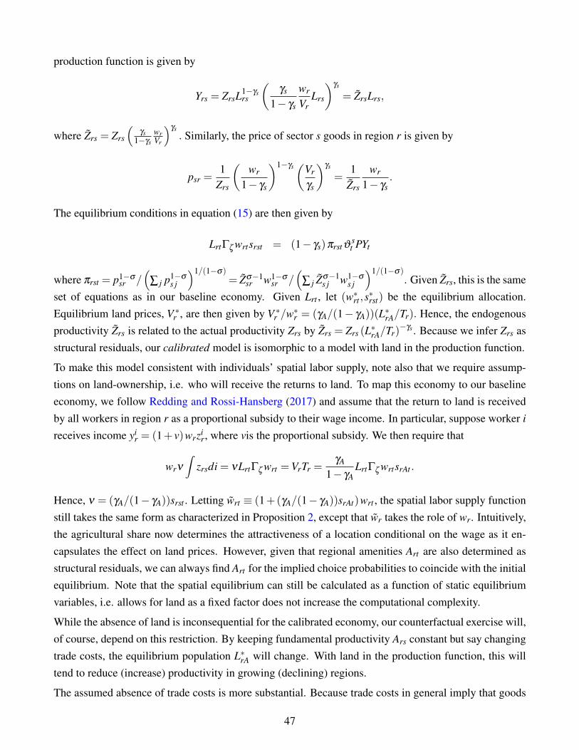
production function is given by

Yrs = ZrsL1−γsrs

(γs

1− γs

wr

VrLrs

)γs

= ZrsLrs,

where Zrs = Zrs

(γs

1−γs

wrVr

)γs. Similarly, the price of sector s goods in region r is given by

psr =1

Zrs

(wr

1− γs

)1−γs(

Vr

γs

)γs

=1

Zrs

wr

1− γs.

The equilibrium conditions in equation (15) are then given by

LrtΓζ wrtsrst = (1− γs)πrstϑst PYt

where πrst = p1−σsr /

(∑ j p1−σ

s j

)1/(1−σ)= Zσ−1

sr w1−σsr /

(∑ j Zσ−1

s j w1−σ

s j

)1/(1−σ). Given Zrs, this is the same

set of equations as in our baseline economy. Given Lrt , let (w∗rt ,s∗rst) be the equilibrium allocation.

Equilibrium land prices, V ∗r , are then given by V ∗r /w∗r = (γA/(1− γA))(L∗rA/Tr). Hence, the endogenousproductivity Zrs is related to the actual productivity Zrs by Zrs = Zrs (L∗rA/Tr)

−γs . Because we infer Zrs asstructural residuals, our calibrated model is isomorphic to a model with land in the production function.

To make this model consistent with individuals’ spatial labor supply, note also that we require assump-tions on land-ownership, i.e. who will receive the returns to land. To map this economy to our baselineeconomy, we follow Redding and Rossi-Hansberg (2017) and assume that the return to land is receivedby all workers in region r as a proportional subsidy to their wage income. In particular, suppose worker i

receives income yir = (1+ v)wrzi

r, where vis the proportional subsidy. We then require that

wrν

∫zrsdi = νLrtΓζ wrt =VrTr =

γA

1− γALrtΓζ wrtsrAt .

Hence, ν = (γA/(1− γA))srst . Letting wrt ≡ (1+(γA/(1− γA))srAt)wrt , the spatial labor supply functionstill takes the same form as characterized in Proposition 2, except that wr takes the role of wr. Intuitively,the agricultural share now determines the attractiveness of a location conditional on the wage as it en-capsulates the effect on land prices. However, given that regional amenities Art are also determined asstructural residuals, we can always find Art for the implied choice probabilities to coincide with the initialequilibrium. Note that the spatial equilibrium can still be calculated as a function of static equilibriumvariables, i.e. allows for land as a fixed factor does not increase the computational complexity.

While the absence of land is inconsequential for the calibrated economy, our counterfactual exercise will,of course, depend on this restriction. By keeping fundamental productivity Ars constant but say changingtrade costs, the equilibrium population L∗rA will change. With land in the production function, this willtend to reduce (increase) productivity in growing (declining) regions.

The assumed absence of trade costs is more substantial. Because trade costs in general imply that goods

47

prices vary across space, consumers’ spatial choice problem will no longer be static. In particular, thespatial choice probabilities are given by (see Propositions 1 and 2 and equation (6))

ρ jrt =exp( 1

κ

(Wrt +Λr,t,t+1−MC jr

))∑

Rl=1 exp

( 1κ

(Wlt +Λl,t,t+1−MC jl

)) , (23)

where Λr,t,t+1 =−ν

γ

((pr

At/prNAt)γ

+β(

prAt+1/pr

NAt+1)γ)+(1+β )(ν/γ−1/η) and pr

st =(

∑ j(τ jr p jst

)1−σ)1/(1−σ)

and τ jr denotes the costs to ship goods from region j to region r. Crucially, the terms Λr,t,t+1 now dependon r and hence no longer drop out of expression (23). This implies that moving flows at time t, dependon the distribution of future regional prices. And as future prices depend on future equilibrium alloca-tions, computing the equilibrium becomes more involved. While in our baseline model, we only need toguess the time path of interest rates, we would now guess and iterate over the entire sequence of futuredistributions of regional factor prices.

Note however, that there are some special case of moving costs, which are covered in our baseline model.In particular, suppose that the final consumption good in equation (2) is the output of a national retailer,who sells to consumers irrespective of their location of residences. For the retailer to procure sector s

goods from region r, however, is subject to trade costs. i.e. τsr ≥ 1 units have to be shipped for a singleunit to reach the retailer. This model is isomorphic to our baseline economy, where effective regional pro-ductivity Qrst is given by Qrst = Qrstτ

−1sr , i.e. lower trade costs are isomorphic to higher productivity. In

Section B.9 below we show that the implied productivities from our model are systematically correlatedwith measures of market access from Donaldson and Hornbeck (2016).

B.2 Proof of Proposition 1

Suppose that the indirect utility function falls in the PIGL class, i.e. V (e, p) = 1η(e/B(p))η +C (p)− 1

η.

The maximization problem is

U ir = max

[et ,et+1,s]{V (et , pt)+βV (et+1, pt+1)} ,

subject to

et + st pI,t = yirt

et+1 = (1+ rt+1)st pI,t+1.

Substituting for et+1 yields

U ir = max

et

{V (et , pt)+βV

((1+ rt+1)

(yi

rt− et) pI,t+1

pI,t, pt+1

)}.

48

The optimal allocation of spending is determined from the Euler equation

∂V (et , pt)

∂e= β (1+ rt+1)

pI,t+1

pI,t

∂V (et+1, pt+1)

∂e.

From above (36) we get that this equation is

eη−1t B(pt)

−η = β

((1+ rt+1)

pI,t+1

pI,t

)η ((yi

rt− et))η−1

B(pt+1)−η .

This yields

yirt− et

et=

((1

1+ rt+1

B(pt+1)/B(pt)

pI,t+1/pI,t

)η 1β

) 1η−1

,

so that

et =1

1+(

φη

t,t+11β

) 1η−1

yirt

et+1 =(1+ rt+1) pI,t+1

pI,t

(φ

η

t,t+11β

) 1η−1

1+(

φη

t,t+11β

) 1η−1

yirt

where φt,t+1 ≡ 11+rt+1

B(pt+1)/B(pt)pI,t+1/pI,t

. Hence, (5) implies that

U jr = Vjr (et , pt)+βVjr (et+1, pt+1)

= A jr1η

wη

rt

B(pt)−η

(1+(

1β

φη

t,t+1

) 1η−1)1−η

+C (pt)+βC (pt+1)−1+β

η.

This can be written as U jr = A jrwη

rtΦt,t+1 +Λt,t+1, where

Φt,t+1 =1η

B(pt)−η

(1+(

1β

φη

t,t+1

) 1η−1)1−η

Λt,t+1 = C (pt)+βC (pt+1)−1+β

η.

For our specification we have that B(pt) = pφ

A,t p1−φ

NA,t = 1. Hence,

φt,t+1 ≡B(pt+1)

B(pt)(1+ rt+1)=

11+ rt+1

= φt+1

49

and

Φt,t+1 =1η

1+(

1β

(1

1+ rt+1

)η) 1η−1

1−η

=1η

(1+β

11−η (1+ rt+1)

η

1−η

)1−η

.

Note also thatet =

1

1+(

φη

t,t+11β

) 1η−1

wt =1

1+β1

1−η (1+ rt+1)η

1−η

wt .

This proves the results for Proposition 1.

B.3 Earning, Expected Earnings and Aggregate Demand

Consider individual i in region r. Given her optimal occupational choice, the earnings of individual i

are given by yi = maxs{

wrszis}. We assumed that individual productivities are Frechet Distributed, i.e.

Fhs (z) = e−Ψh

s z−ζ

, where Ψhs parametrizes the average level of productivity of individuals of skill h in

region r in sector s and ζ the dispersion of skills. Hence, the distribution of sectoral earning yirs ≡wrszi

s isalso Frechet and given by Fyrs (y) = P

(z≤ y

wrs

)= e−Ψh

s wζrsy−ζ

. Using standard arguments about the maxstability of the Frechet, the distribution of total earnings yi is also Frechet and given by

Fhyr(y) = e−(Θh

r)ζ

y−ζ

= e−(

yΘh

r

)−ζ

(24)

where Θhr =

(∑s Ψh

s wζrs

)1/ζ

=(

ΨhAwζ

rA +ΨhNAwζ

rNA

)1/ζ

. Hence, average earnings of individual i with

skill type h in region r are given by E[yi

r,h

]= Γ

(1− 1

ζ

)Θh

r . From (24) we can derive the distribution of

y1−η . As η < 1, we have that

Fy1−η (q) = P(y1−η ≤ q

)= P

(y≤ q1/(1−η)

)= e

−Θζ

(q

11−η

)−ζ

= e−(

qΘ1−η

)− ζ

1−η

.

Hence, y1−η is still Frechet. Therefore

∫iy1−η

i di = Lhr E[y1−η

i

]= Lh

r Γ

(1− 1−η

ζ

)(Θ

hr

)1−η

= Lhr Γ

(1+

η−1ζ

)(Θ

hr

)1−η

.

To derive the aggregate value added share ϑ At , note that

PY At =

R

∑r=1

(ϑA

(ES Y

r, p)

ES Yr

Lrt +ϑA

(ES O

r, p)

ES Or

Lrt−1

)+φ It

= φ

[It +

R

∑r=1

(ES Y

rLrt +ES O

rLrt−1

)]+ ν

(pA

pNA

)γ R

∑r=1

(E1−η

S Yr

Lrt +E1−η

S Or

Lrt−1

).

50

Now note that total spending of the old equals the capital return plus the non-depreciated stock of capital,i.e.

R

∑r=1

ES Or

Lrt−1 = RtKt +(1−δ )Kt = αPYt +(1−δ )Kt .

And because the future capital stock is given by the savings of the young generation (see (19)), we getthat

It +R

∑r=1

(ES Y

rLrt +ES O

rLrt−1

)= Kt+1 +

R

∑r=1

(ES Y

rLrt

)+αPYt = PYt .

This yields (14).

B.4 The Quasi-Spaceless Economy

If wages are equalized across space, wrt = wt , the final good prices are given by

pst =

R

∑r=1

(1

QrstZst

(wt

1−α

)1−α(Rt

α

)α)1−σ

11−σ

=1

Zst

(wt

1−α

)1−α(Rt

α

)α

,

as ∑Rr=1 Qσ−1

rst . Hence, the choice of numeraire implies that

1= pφ

At p1−φ

NAt =

(1

ZAt

)φ ( 1ZNAt

)1−φ ( wt

1−α

)1−α(Rt

α

)α

=

(1

ZAt

)φ ( 1ZNAt

)1−φ(

PYt

∑Rr=1 LrtΓζ

)1−α(PYt

Kt

)α

.

Hence, PYt =ZtKαt L1−α where Zt =Γ

1−α

ζZφ

AtZ1−φ

NAt and L=∑r Lr. Using that Kt+1 =(1−ψt+1)(1−α)PYt ,the expression for ψt+1, rt = Rt−δ and kt = Kt/L, we get that

kt+1

((1β

) 11−η (

1+αZt+1k−(1−α)t+1 −δ

)− η

1−η

+1

)= (1−α)Ztkα

t .

Note that the LHS is increasing and continuous in kt+1 and satisfies limkt+1→∞ LHS=∞ and limkt+1→0 LHS=

0. Hence, there is a unique mapping kt+1 = m(kt ,Zt ,Zt+1) . Furthermore, m(.) is increasing in all argu-ments.

B.5 The Equilibrium with Heterogeneous Skills

The equilibrium characterization for the case of heterogenous skills is very similar to our baseline case.In that case, the spatial equilibrium, i.e. the set of equilibrium wages and population levels {wrt ,Lrt}rt ,

51

is determined from labor market clearing condition (17)

LrtΓζ wrt = (1−α)(

πrAtϑAt +πrAt

(1−ϑ

At

))PYt

and the spatial labor supply condition Lrt = ∑Rj=1 ρ jrtL jt−1, where ρ jrt , ϑ A

t and πrst are given in (12), (14)and (16) and also only depend on {wrt ,Lrt}r. Given {wrt ,Lrt}r, the future capital stock is then determinedfrom (19) and the regional agricultural employment shares from expression (18).

In the case with sector-specific skills and imperfect substitutability, the spatial equilibrium consists ofsector-specific wages {wrAt ,wrNAt}r and skill-specific populations

{LL

rt ,LHrt}

r. The corresponding equi-librium conditions are as follows. The regional labor market clearing condition is given by

LrtΓζ

(λrtΘ

Hrt +(1−λrt)Θ

Lrt)= (1−α)

(πrAtϑ

At +πrAt

(1−ϑ

At

))PYt ,

where Θhr , given in equation (21), denotes regional income for skill group h and λrt is the share of

skilled individuals.36 The labor supply equations are now skill-specific and given by Lhrt =∑

Rj=1 ρh

jrtLhjt−1,

where ρhjrt is still given in (12) with W h

rt =(Γη/ζ/η

)ψ (rt+1)

η−1 (Θh

r)η

+Art . Finally, the within-regionallocation of factors across sectors, i.e. the counterpart to (18), is given by

πrAt

πrNAt

ϑ At

1−ϑ At=

wrA(HL

rA +HHrA)

wrNA(HL

rNA +HHrNA

) = ( wrAt

wrNAt

)ζ (1−λr)ΨLA(Θh

r)1−ζ

+λrΨHA(ΘH

r)1−ζ

(1−λr)ΨLNA

(Θh

r)1−ζ

+λrΨHNA (Θ

Hr )

1−ζ. (25)

These equations determine{

wrAt ,wrNAt ,LLrt ,L

Hrt}

r. The skill specific employment shares can then be

calculated as shrst = Ψh

s(wrs/Θh

r)ζ

. The capital accumulation is still given by (19), i.e.

Kt+1 = (1−ψ (rt+1))∑r

LrtΓζ

(λrtΘ

Hrt +(1−λrt)Θ

Lrt)= (1−ψ (rt+1))(1−α)PYt .

The main difference to the case with substitutable skills is the within-region sectoral supply equation(25). In the baseline model, srAt is determined residually from equation (18). With an upward slopingsupply curve, the relative wages have to be consistent with sectoral labor supplies.

B.6 Balanced Growth Path Relationships

Consider a dynamic allocation where GDP grows at a constant rate g and the capital output ratio isconstant. Static optimality requires that Rt = αPYt/Kt . Hence, a constant capital output ratio directlyimplies that the return to capital Rt has to be constant. Hence, the real interest on saving is also constantand given by r = R−δ . This also implies that the consumption rate in equation (10) is constant and given

36To see that, note that labor earnings in region r, for skill group h in sector s are given by wrstHhrst = LrtΓζ λ h

r shrsΘ

hr .

Summing over sectors s and skill groups h yields the expression above.

52

by

ψ =(

1+β1

1−η (1+ r)η

1−η

)−1. (26)

To solve for the interest rate, note that capital grows at rate g, so that expression (19) implies that

Kt+1

Kt=

(1−ψ)(1−α)PYt

αPYt/R= (1−ψ)

(1−α)

α(r+δ ) = 1+g.

Hence,

1+g = (1−ψ)(1−α)

α(r+δ ) =

(β

11−η (1+ r)

η

1−η

1+β1

1−η (1+ r)η

1−η

)(1−α)

α(r+δ ) . (27)

This equation determines r as a function of parameters. Along the BGP the consumption and investmentrate is equal to

PCt = ψ (1−α)PYt +αPYt +(1−δ )α

RPYt =

[ψ (1−α)+α +(1−δ )

α

R

]PYt

PIt = (1−ψ)(1−α)PYt− (1−δ )α

RPYt =

[(1−ψ)(1−α)− (1−δ )

α

R

]PYt

Using equation (27) yields (PIt/PYt) = (g+δ )(α/R) and PCt/PYt = 1− (g+δ )(α/R). From equation(27) we also get that ψ = (α/(1−α))(1+g/R).

B.7 Regularity conditions for PIGL preferences

In our model, expenditure share on the two goods are given by

ϑA (e, p) = φ +ν

(pA

pNA

)γ

e−η

ϑNA (e, p) = 1−φ −ν

(pA

pNA

)γ

e−η .

For these expenditure shares to be positive, we need that

ϑA (e, p)≥ 0⇒ eη ≥−ν

φ

(pA

pNA

)γ

, (28)

and ϑNA (e, p) ≥ 0⇒ eη ≥ (ν/(1− φ))(pA/pNA)γ . Note first that (28) is trivially satisfied as long as

ν > 0. Also note that satisfying both of these restrictions automatically implies that ϑs (e, p) ≤ 1. Inaddition, as we show in Section C.3 in the Online Appendix, for the Slutsky matrix to be negative semidefinite, we need that

53

ν (1−η)

(pA

pNA

)γ

− (1−φ)φ

ν

(pA

pNA

)−γ

e2η ≤ (1−2φ − γ)eη .

Hence, for our preferences to be well-defined, we require that

eη ≥ ν

1−φ

(pA

pNA

)γ

(29)

(1−2φ − γ)eη +(1−φ)φ

ν

(pA

pNA

)−γ

e2η ≥ ν (1−η)

(pA

pNA

)γ

. (30)

Lemma 5. A sufficient condition for (29) to be satisfied is that (30) holds and that

γ > (1−φ)η . (31)

Proof. Equation (30) can be written as eη

ν

1−φ

(pA

pNA

)γ −1

+φeη

ν

1−φ

(pA

pNA

)γ

eη

ν

1−φ

(pA

pNA

)γ ≥ [(1−φ)(1−η)−1]+ (2φ + γ)eη

ν

1−φ

(pA

pNA

)γ .

Letting x = eη

ν

1−φ

(pA

pNA

)γ , this yields

(x−1)+(φx− (2φ + γ))x≥−(1− (1−φ)(1−η)) .

Now let h(x) = (x−1)+(φx− (2φ + γ))x. For (30) to be satisfied we need that

h(x)≥−(1− (1−φ)(1−η)) .

Note that h is strictly concave with a minimum at

h′ (x∗) = 1+φx∗− (2φ + γ)+φx∗ = 0.

Hence,x∗ = 1− 1− γ

2φ< 1.

Also note thath(0) =−1 <−(1− (1−φ)(1−η)) .

Hence, for condition (30) to be satisfied, it has to be the case that x > x∗ = 1− ((1− γ)/2φ) as h(x∗)<

h(0). Hence, condition (30) implies inequality (29) if

h(1) = φ −2φ − γ <−(1− (1−φ)(1−η)) .

54

Rearranging terms yields (1−φ)η < γ , which is inequality (31).

Hence, the preferences are well defined as long (30) is satisfied and (31) holds. Because the RHS of (30)is increasing in e in the relevant range, i.e. as long as (30) is satisfied, this implies that the preferencesare well defined as long as e is high enough.

Now note that eit = ψt+1yit , where yit denotes total earnings of individual i. From (24) we know that

P(eit ≤ κ) = P(

yit ≤κ

ψt+1

)= e−(Θh

r ψt+1)ζ

κ−ζ

,

where

(Θ

hrtψt+1

)ζ

=(

ΨhAwζ

rAt +ΨhNAwζ

rNAt

)ψ

ζ

t+1 >(

ΨhAwζ

rAt +ΨhNAwζ

rNAt

)( 1η

(1+β

11−η

)1−η)ζ

.

Hence, as long as aggregate productivity in 1880 (and hence wrs1880) is high enough, we can makeP(eit ≤ κ) arbitrarily small.

B.8 Additional Properties of the Calibrated Model

In this section we provide additional results for the fit of the calibrated model.

Migration by skill type In the model low and high skill workers are subject to the same distance costs,which yields an elasticity of moving flows to distance that is very similar for both groups. As the leftpanel of the below figure shows this is in line with the data. In the model high skill types are slightly morelikely to move but not a lot. In the data low skilled workers are substantially less likely to leave their birthstate. The model can match if we allowed τ to differ by skill type, since as outlined in the calibrationsection, the total number of stayers is monotone in τ . We chose to abstract from this for simplicity in themain part of the paper.

Moving costs To quantify the economic magnitude of our estimated fixed costs, we calculate

∆hjt ≡

U h,Movjt −U h,Stay

jt

τ, (32)

i.e. the average increase in utility by moving relative to the fixed cost of moving as a norm for theeconomic magnitude of fixed costs. Because utility is not equalized, these gains differ by commutingzone. In Table 9 we report some statistics of the distribution of ∆h

jt . In the top row we report thesestatistics for low skilled individuals, in the bottom row for high skilled individuals. Table 9 shows thatfor the median commuting zone the expected value of moving is slightly positive and amounts to roughly5% (10% for high skilled individuals) of the estimated fixed cost of moving.

55

Low SkillHigh Skill-1

0

1

2

3

Log

Inte

rsta

te F

low

s

0 .2 .4 .6 .8 1Normalized Distance

High Skill Low Skill

.5

1

1.5

2

2.5

0 .2 .4 .6 .8 1Fraction of Stayers by Skill 1910-1940 (States)

Notes: To construct the left panel, we run a gravity equation of the form where origin and destination fixed effects are skill specific:lnρ jr/(1−ρ j j

)=

αhj +αh

r + uhjr . The red diamonds line plots the resulting uH

jr by distance percentile, the blue line does the same for low skill types. The right panel we plotthe distribution of the share of people staying in their home state between 1910 and 1940 for low and high skilled workers.

Figure 12: Lifetime Interstate Migration by Skill in 1940 in the Data

Expected value of moving relative to fixed costs ∆hjt

10% 25% 50% 75% 90%Low Skilled -0.2543 -0.0937 0.0571 0.1900 0.2871High Skilled -0.2464 -0.0654 0.1065 0.2543 0.3619

Notes: The table reports different quantiles of the distribution of ∆hjt calculated as (32).

Table 9: The Economic Magnitude of Moving Costs

Regional Fundamentals In this section, we describe additional details for the estimated spatial pro-ductivities {QrAt ,QrNAt}rt and amenities {Art}rt . First we we study the fundamental determinants ofagricultural specialization by projecting the endogenous agricultural employment share on regional fun-damentals and the two state variables of the system, namely the distribution of skills and population sizein 1880. We do so in Table 10. In particular, we report the results from the specification

lnsrAt = δt +βNAlnQrNAt +βAlnQrAt + γArt +ζ λr1880 +η lnpopr1880 +urt ,

where δt is a year fixed effect. In columns 1 to 3 we report the bivariate partial correlations. Rural, agri-cultural regions are regions with low productivity in the non-agricultural sector, a comparative advantagein the production of agricultural goods and low amenities. The last column reports the respective partialcorrelations. In particular, the coefficient on regional amenities and the regional skill share drops by afactor of ten. This reflects the existing cross-sectional correlation with regional productivity, in particularnon-agricultural productivity QrNA.

In Table 11 we focus directly on the dynamics of spatial productivity and amenities. In particular, weconsider a simple autoregressive specification

xrt = δt +δr +βyrt−1 +urt

56

Dep. variable: lnsArt

Non Ag. Productivity (lnQrNA) -0.331∗∗∗ -0.344∗∗∗

(0.020) (0.007)

Ag. Productivity (lnQrA) 0.404∗∗∗ 0.408∗∗∗

(0.022) (0.006)

Amenities (Ar) -0.430∗∗∗ -0.055∗∗∗

(0.075) (0.013)

Skill share in 1880 (λr1880) 0.139 -1.594∗∗∗ -0.466∗∗ -0.117∗∗∗

(0.123) (0.150) (0.196) (0.032)ln population 1880 X X X XYear FE X X X XN 3225 3225 2580 2580R2 0.891 0.902 0.810 0.989

Notes: Robust standard errors in parentheses with ∗∗∗, ∗∗ and ∗ respectively denoting significance at the 1%, 5% and 10% levels. All specification control forthe population in 1880 and for year fixed effects.

Table 10: Fundamental Determinants of Agricultural Specialization

lnQrNAt lnQrAt Art

lnQrNAt−1 0.832∗∗∗ 0.416∗∗∗

(0.011) (0.039)lnQrAt−1 0.725∗∗∗ 0.045

(0.050) (0.043)Art−1 0.897∗∗∗ 0.175

(0.063) (0.133)Year FE X X X X X XCZ FE X X XN 2580 2580 2580 2580 1935 1935R2 0.907 0.958 0.486 0.789 0.749 0.890

Notes: Robust standard errors in parentheses with ∗∗∗, ∗∗ and ∗ respectively denoting significance at the 1%, 5% and 10% levels.

Table 11: The Process of Spatial Fundamentals

where x denotes either log sectoral productivity, lnQrst , or the level of amenities Art and δt and δr areregion and year fixed effects. The first four columns show that productivities are mean-reverting and thatthere is an important fixed, region-specific component determining spatial productivity between 1880 and2000. It is also interesting to note that these patterns differ slightly across sectors. In particular, condi-tional on commuting zone fixed effects, past agricultural productivity is uncorrelated contemporaneousagricultural productivity.The last two columns show the same result for regional amenities. Amenitiesfollow a stochastic process, which is similar to agricultural productivity.

B.9 Local Productivities and Market Access

We calibrate the cross-sectional distribution of sectoral productivities {QrAt ,QrNAt}rt and amenities {Art}rt

as structural residuals of the model as is commonly done in the new quantitative spatial economics liter-

57

ature (see (Redding and Rossi-Hansberg, 2017) for a recent and excellent review of this literature). Thelocal sectoral productivities calibrated this way, {QrAt ,QrNAt}rt , are residuals necessary to fit the data onwages and sectoral employment conditional on the calibrated parameters of the model. While they reflecta variety factors that make one region more productive than another, some measurable others not, thereis one factor that determines the productivity of a location in a very direct way: its integration into thenational transportation network. In this section we use direct measures on the extent of regional “marketaccess” by Donaldson and Hornbeck (2016) for each county in the US for 1880 and 1910 to corroborateour model-based measures of regional productivity.

Donaldson and Hornbeck (2016) provide data on county-to-county transport cost for 1880 and 1910. Weuse this data to construct a commuting zone level index for market access costs for these time periods. Inparticular we average the market access cost across all county-to-county pairs within two given commut-ing zones to obtain a measure for the ease of transporting goods between these two zones. Then we takethe destination population share weighted sum of market access cost for each origin commuting zone toobtain our market access index at the commuting zone level.

We now relate this index of market access costs to our measured regional productivity residuals Qrst .Letting MACrt be this index of market access costs of county r at time t, we consider a specifications of

lnQrst = δr +β ×MACrt +urst , (33)

where δr denotes a fixed effect at different levels of regional aggregation. We expect β < 0, as highertransport costs should reduce a county’s earnings potential, i.e. productivity. We estimate 33 separatelyfor the agricultural and the non-agricultural sector. The results are contained in Table 12.

In the first two columns we show that our model infers low productivity in places that have a highmarket access cost. Columns 3 and 4 show that this relationship is if anything stronger within states. Incolumns 5 and 6 we exploit the time-variation within commuting zones and show that regions who seetheir access costs decrease indeed experience faster productivity growth. Finally, in the last two column,we estimate 33 in first differences and explicitly include a whole set of state fixed effects, i.e. allowingfor systematic differences in productivity growth across states. Again, we find a significant relationshipbetween (changes in ) market access costs and (changes in) regional productivity. We take this as evidencethat transportation costs are one of the directly measurable ingredients in regional productivity shiftersthat our framework infers as {QrAt ,QrNAt}rt .

58

lnQrNAt lnQrAt lnQrNAt lnQrAt lnQrNAt lnQrAt ∆ lnQrNAt ∆ lnQrNAtMarket Access Costs -1.897∗∗∗ -2.077∗∗∗ -5.205∗∗∗ -4.291∗∗∗ -3.937∗∗∗ -3.760∗∗∗

(0.224) (0.125) (0.290) (0.195) (0.353) (0.309)Change in Market Access Costs -4.005∗∗∗ -2.395∗∗∗

(0.388) (0.328)Year FE X X X XCZ FE X XState FE X X X XN 1242 1242 1242 1242 1242 1242 621 621adj. R2 0.133 0.286 0.538 0.455 0.789 0.576 0.337 0.399

Notes: Robust standard errors in parentheses with ∗∗∗, ∗∗ and ∗ respectively denoting significance at the 1%, 5% and 10% levels. We measure Market AccessCosts using the data from Donaldson and Hornbeck (2016). We use data on the cost of reaching any other county from a given county, take the destinationpopulation weighted sum and aggregate them to the commuting zone level. Our measure of market access costs is the log of this index. The change in marketaccess costs is the log difference between 1880 and 1910.

Table 12: Spatial Productivity and Market Access Cost from Donaldson and Hornbeck (2016)

B.10 Spatial Welfare Inequality

In Table 5 in the main text we discuss the evolution of spatial inequality. We construct this the numbersin this table in the following way. From Proposition 2 we have that expected utility in region r is givenby

W hrt

(Θ

hr

)=

Γη/ζ

ηψ (rt+1)

η−1(

Θhr

)η

+Λt,t+1 +Art . (34)

Let T hrt (∆) be the increase in average income Θh

r required to increase utility by ∆, i.e. W hrt(Θh

r T hrt (∆)

)=

W hrt(Θh

r)+∆. (34) implies that

T hrt (∆) =

1+∆

Γη/ζ

ηψ (rt+1)

η−1 (Θh

r)η

1/η

.

Let ∆h,IQRt be the interquartile range in regional welfare W h

rt at time t, i.e. ∆h,IQRt =W h,75

t −W h,25t , where

W h,xt is the x-quantile of the distribution of W h

rt .

B.11 Agricultural Employment Shares and Skilled Employment

The 1940 cross-section of the US Micro Census published by the US Census Bureau is the first to containan educational variable and the last to contain the full set of county identifiers. We construct skilledemployment shares on the county level as the fraction of workers employed in this county that have atleast a completed high school degree. In Figure 13 we depict the spatial correlation between agriculturalemployment shares and skill shares. The calibration strategy outlined in the main body of the paperallows us to match the distribution of skilled employment shares in 1940 exactly.

59

.1

.15

.2

.25

.3

.35

Reg

iona

l Ski

lled

Empl

oym

ent S

hare

194

0

0 .2 .4 .6 .8Regional Agricultural Employment Share 1940

Notes: The figure shows the binscatter plot of the agricultural employment shares in US counties and their skilled employment shares in 1940.

Figure 13: Agricultural Employment Shares and Skilled Employment Shares in 1940

60