SPATIALIZING SOCIAL NETWORKS: MAKING SPACE FOR THEORY IN SPATIAL ANALYSIS

BY STEVEN MATTHEW RADIL

DISSERTATION Submitted in partial fulfillment of the requirements

for the degree of Doctor of Philosophy in Geography in the Graduate College of the

University of Illinois at Urbana-Champaign, 2011

Urbana, Illinois

Doctoral Committee: Associate Professor Colin Flint, Chair Professor Sara McLafferty Assistant Professor Julie Cidell Associate Professor George Tita, University of California, Irvine

ii

ABSTRACT

This study is a quantitative and spatial analysis of the gang-related violence in a

section of Los Angeles. Using data about the spatial distribution of gang violence in three

neighborhoods of Los Angeles, this research first adopts a deductive approach to the

spatial analysis of gang violence by spatial regression models that considers the relative

location of the gangs in space while simultaneously capturing their position within a

social network of gang rivalries. Several models are constructed and compared and the

model that seems to best fit the observed geography of violence is one in which both the

territorial geography and the social geography of the gangs is utilized in the

autocorrelation matrix. Building on the findings of the spatial regression modeling, the

concept of social position and associated techniques of structural equivalence in social

network analysis is then explored as a means to integrate these different spatialities. The

technique of structural equivalence uses the two different spatialities of embeddedness to

identify gangs that are similarly embedded in the territorial geography and positioned in

the rivalry network which aids in understanding the overall context of gang violence. The

importance of theory to guiding spatial regression modeling is demonstrated by these

findings and the hybrid spatial/social network analysis demonstrated here has promise

beyond this one study of gang crime as it operationalizes spatialities of embeddedness in

a way that allows simultaneous systematic evaluation of the way in which social actors’

position in network relationships and spatial settings provide constraints and possibilities

upon their behavior.

iii

To Jennifer, Maxwell, and Kira.

iv

ACKNOWLEDGEMENTS

This dissertation is more than just the product of my own efforts and I owe a debt

of gratitude to a great number of people. I first offer my thanks to the people whom

encouraged me to pursue a PhD in geography while I was working on my Master’s

degree, particularly Professors Eve Gruntfest and John Harner. I owe a special debt of

gratitude to my Master’s advisor, Professor Roger Sambrook. His confidence and support

has been constant as I continued the academic journey that I began under his tutelage.

I am extremely grateful for the contribution and guidance provided by my

committee members, Professors Sara McLafferty, Julie Cidell, and George Tita. Their

support, suggestions, and collaborations during my time at Illinois have helped me find

my way through the process of completing my dissertation. I am especially grateful for

their flexibility and willingness to help me find my own path with my research. In nearly

every way, this dissertation would not have been possible without the unwavering

support and generosity of Professor Tita. What began as a simple request for data turned

into an ongoing research partnership for which I am extremely grateful. Collaborating

with George has made me a better scholar and I have encountered no better role model

for my professional career. I would also like to thank Professors Paul Diehl and Shin Kap

Han for their thorough and careful contributions during my preliminary exams. Finally,

thanks to the many faculty who employed me in some capacity (Professors Julie Cidell,

Colin Flint, and Courtney Flint), offered their insight through independent study

(Professors Colin Flint, Jurgen Scheffran, Sara McLafferty, and Paul Diehl), or guided

me and collaborated with me on research projects (Professors Colin Flint, George Tita,

Paul Diehl, John Vasquez, and Jurgen Scheffran).

v

While at Illinois I have had two homes: the Geography Department and the

Program for Arms Control, Disarmament, and International Security (ACDIS). I would

like to thank the Geography Department staff, Susan Houston and Susan Etter, for their

repeated help and support. I especially offer my earnest thanks to Kathy Anderson-

Conner at ACDIS. She is a true professional and I thank her for making me welcome

when I first arrived at ACDIS and for helping me stay productive and engaged since.

In addition to my dissertation committee members, other faculty, and Geography

and ACDIS staff at Illinois, I want to acknowledge several of my fellow PhD students for

their consistent friendship, support, and professionalism. I thank Matt Anderson and

Robert Cochrane for their excellent work in the classroom in Geography 110 with a

special thanks to Matt for showing me the ropes during my first semester as a TA.

Thanks as well to my excellent office mates at Davenport, Miriam Cope and Ben Cheng,

for putting up with the long lines of undergraduate students during my office hours. I will

dearly miss sharing an office with Miriam as her thoughtfulness and passion about her

own work (and mine) is an inspiration. I also thank the many graduate students associated

with the ACDIS program (too many to name here) that have formed a second social

community for me around our shared academic interests.

Of all the excellent graduate students I have encountered at Illinois, I have found

a consistent source of inspiration and close friendship among my fellow Political

Geographers: Andy Lohman, Sang-Hyun Chi, Richelle Bernazzoli, Jongwoo Nam, and

Erinn Nicely. In many ways, each has inspired me and strongly shaped my own work,

perhaps without them fully knowing it. I’m so grateful to have had the opportunity to

know each of them and look forward to many years of continued friendship and

vi

professional collaboration. I especially thank Andy, Richelle, and Sang-Hyun for their

friendship and support. In hindsight, I think it would not have been possible to finish this

journey without the presence of outstanding friends and colleagues such as these.

It is difficult to put into words how grateful I am to my advisor, Professor Colin

Flint. He is, simply put, the person I most deeply admire in my professional life and his

friendship and mentoring have forever altered my life and career for the better. Apart

from my family, the experience of being his student has been perhaps the most rewarding

of my life. After leaving Illinois, I can think of no higher praise than to strive to emulate

Colin’s commitment to his students and his profession. I can not thank him enough for

his guidance and friendship.

Lastly, I could have never accomplished this goal without the support of my

family and friends. I thank my wife Jennifer for her love and support during this

sometimes bumpy journey. Between the two of us, Jennifer has perhaps shouldered the

heaviest load during our time here and has done so with consistent grace and good humor

while keeping one eye on the next phase of our lives. Our children Maxwell and Kira

have largely grown up so far with their father in graduate school and their unconditional

love and support have made my path easier while also reinforcing my determination to

finish as soon as possible. Finally, thanks to my parents, my step parents, and to

Jennifer’s parents. Each has unconditionally supported our goals, even when that meant

increasing the geographic distance between us in order to pursue those goals.

vii

TABLE OF CONTENTS

CHAPTER 1: INTRODUCTION ....................................................................................1 CHAPTER 2: SPATIAL REGRESSION MODELS IN CRIMINOLOGY.....................13 CHAPTER 3: THEORIZING SPACE AND PLACE FOR SPATIAL ANALYSIS IN CRIMINOLOGY...........................................................45 CHAPTER 4: MODELING SOCIAL PROCESS IN THE SPATIAL WEIGHTS MATRIX ..............................................................................65 CHAPTER 5: SPATIALIZING SOCIAL NETWORKS: GEOGRAPHIES OF RIVALRY, TERRITORIALITY, AND VIOLENCE.......................109 CHAPTER 6: CONCLUSIONS...................................................................................153 REFERENCES............................................................................................................162

1

CHAPTER 1

INTRODUCTION

The recognition of geography as a factor in the explanation of a multitude of

social phenomena has been an increasingly notable component of quantitative social

science (Goodchild et al. 2000). Research produced in a variety of disciplines now

incorporates geographic or spatial elements into analysis that utilizes quantitative

methodologies. An important reason for the adoption of spatial perspectives for

quantitative social science has been a growing recognition of the importance of context to

human action. As Flint (2002: 34) argues, spatial perspectives are now important in social

science because “people with similar socioeconomic and cultural characteristics are likely

to behave differently within unique contextual settings” and incorporating context into

quantitative models of human behavior is the ongoing focus of the subfield of spatial

analysis and spatial statistics within human geography.

The analysis of spatial phenomena in social science has been made possible in

recent years by the ongoing development of statistical techniques that attempt to deal

with some of the unique problems of spatial data, especially spatial dependence.

Dependence, or the tendency of characteristics of a given location to correlate with those

of nearby locations, is a foundational issue in quantitative geographical analysis (e.g.,

Anselin 1988; Cliff and Ord 1981; Cressie 1993; Griffith 1987; Haining 1990, 2003).

These methods, commonly called spatial econometrics, were once of interest to a small

set of spatial statisticians and quantitative geographers. However, spatial econometric

models that deal with dependence are now increasingly of interest to large numbers of

researchers from diverse disciplines investigating a wide range of issues (e.g., Ward and

2

Gleditsch 2008). Many social scientists now view spatial econometric regression models

as an improvement on non-spatial techniques as a result of the growing recognition that

dependencies in the spatial structure of research data may limit the inferences of

quantitative investigations (Anselin et al. 2004).

Spatial econometric regression models demand a careful consideration of both the

theoretical and empirical spatial structure of the data in question (e.g., Florax and Rey

1995). However, the advent of new spatial econometric software packages has lowered

the traditional technical barriers to the use of these techniques while simultaneously

making it easy for users to choose among a few predefined spatial structures.1 New users

may therefore be unfamiliar with the importance of the formal spatial structure to analytic

outcomes and less likely to carefully consider their choice (see Leenders 2002). The

small literature new users may draw upon to understand this issue remains quite technical

in nature, even when proclaiming the opposite intent (e.g., Griffith 1996). Taken as a

whole, this state of affairs is less than ideal and unlikely to encourage careful thinking

about space. However, the need to formalize the empirical spatial structure of the data for

modeling is also an opportunity to reflect on the theoretical interaction of the geography

and social processes being studied. In this manner, spatial analyses of human behavior

and outcomes is at the core of the emerging “spatially integrated social science”

identified by Goodchild et al. (2000), and an opening for the investigation of how human

behavior and space are mutually constituted.

1 Examples of spatial econometric software include The “GeoDa” software package (see Anselin et al. 2006 and https://www.geoda.uiuc.edu/) and the "spdep" package in the open source R environment (see Bivand 2002). GeoDa allows users to create spatial weight matrices from data created in a geographic information system (GIS) and spdep will read in matrices created in GeoDa.

3

In light of this state of affairs, this dissertation has a twin purpose. First, I attempt

to build upon the current energy in spatial analytical modeling across social science to

offer a unique contribution by demonstrating the importance of incorporating theory

about the phenomenon of interest into spatial modeling efforts. Second, I offer a new

methodological approach to incorporating theory into spatial modeling. The chapters that

comprise this dissertation are drawn from a series of publications directly related to these

twin goals using data on the production of a particular kind of violence in an urban

context. This dissertation examines gang-related violence within a small area of the city

of Los Angeles and each chapter focuses on a particular element or challenge involved in

producing a theoretically informed spatial analysis using the same data and issue.

RESEARCH PROBLEM

As typically argued in many geographic literatures and, increasingly, in other

social science literatures, spatial perspectives are important for both theoretical and

practical reasons. Theoretically, spatial perspectives are of interest because of the

“longstanding interest in the social production of space” in geography (Cox et al. 2008:

6). Following Lefebvre’s (1991) understanding of space as both social process and social

product, the spatial structures of a given phenomena are commonly investigated as

underlying cause, constructed outcome, or both. For example, the perception of rivalries

over territorial control between a set of gangs and the actual construction of bounded turf

are simultaneously social and geographic phenomena. The competitions are inseparable

from the geography and vice versa. Hence modeling a social process such as gang rivalry

requires modeling the social construction of spaces (Flint 1998).

4

On the other hand, consideration of geography is a practical methodological

matter. Data with a geographical component has important implications for statistical

analyses; if processes that are affected by the underlying spatial structure in a study area

are not accounted for, inferences will be inaccurate and estimates of the effects of

independent variables may be biased (Anselin 1988). Perhaps the most important reason

for the interest in quantitative spatial methods is the most straightforward: nearly all

social science data is spatially organized and ignoring this structural element is

increasingly seen as untenable (Ward and Gleditsch 2008). To accommodate these issues,

statistical models have been developed that attempt to deal with issues of spatial

dependence. Conventionally, this is done through either introducing an additional

covariate (referred to as a ‘spatial lag’ variable which is a weighted average of values for

the dependent variable in areas defined as ‘neighbors’) or by specifying a spatial

stochastic process for the error term. These models are now seen as both viable and

important for social science research (Ward and Gleditsch 2008).

These models have been discussed and exemplified in depth (see Anselin 2002 for

an overview) but an essential element of these models remains largely ignored in the

literature, despite the major theoretical and methodological implications. Both the lag and

error models attempt to estimate regression parameters in the presence of presumably

interdependent variables (Anselin 1988; Leenders 2002). This estimation process requires

the analyst to define the form and limits of the interdependence and formalize the

influence one location has on another. In practice, this is accomplished by identifying the

connectivity between the units of the study area through a nn× matrix. The matrix is

5

usually described in the literature as a ‘spatial weight’ or ‘spatial connectivity’ matrix and

referred to in the preceding lag and error models as “W”.

This W, or matrix of locations, formalizes a priori assumptions about potential

interactions between different locations, defining some locations as influential upon a

given location and ruling others out. A simpler way of describing this is that W identifies,

in some cases, who is a neighbor and who is not, or with whom an actor interacts.

However, the construction of W is more than just an empirical choice about neighbors. It

is a theoretical decision regarding the spatiality of the social processes being discussed

and one that has implications for the statistical estimates generated.

As W is supposed to represent a formal model of connections between geographic

locations, how one translates theories about influence and its mechanisms across space

into a formal mathematical construct is an important step. Put another way, at its core, W

is really a theoretical geography of interaction. However, as a practical matter, the spatial

analytic geography literature focuses on modeling interaction through a distance-based

logic that typically takes one of two forms: contiguity or distance (Cliff and Ord 1981;

Griffith 1996). Both of these spatial themes have been mobilized for constructing W’s for

various kinds of measures of spatial autocorrelation dating back to Cliff and Ord’s

seminal work (1981). Contiguity, or the physical connections between locations, is

emphasized in issues that focus on areal spaces, especially ecological studies that use

aggregated data. Distance between locations of interest remains an important concept to

many kinds of geographic literatures. In the case of issues of society and space, the

6

geography of influence is typically imagined and implemented in the models as a kind of

gradient that uniformly diminishes with increasing distance.2

The development and dissemination of spatial analytic software allows users to

easily create W’s from spatially organized data using the classic spatial forms of areal

contiguity or point-to-point distance. And while such software often guides researchers

through the practical steps needed to create a theoretical geography of spatial interaction

or influence, there is no drop-down menu to offer guidance as to how best to capture the

geography, or spatiality, of the social processes being analyzed. For any given research

topic, are immediately contiguous areal neighbors enough, or should more distant

neighbors also be included? If distance matters, at what distance does influence begin to

diminish? More to the point, why and in what way does distance “matter” in the

operation of the social process under investigation? These questions remain the key

challenges for a theoretically informed spatial analysis.

Somewhat surprisingly, discussions about the nature of W and how different

specification choices may affect regression results have also been underemphasized in

most spatial analytic literature: the relatively few examples to the contrary include Florax

and Rey (1995) and Griffith (1996). Despite these noteworthy efforts, Leenders is correct

in his assessment that “the effort devoted by researchers to the appropriate choice of W

pales in comparison to the efforts devoted to the development of statistical and

mathematical procedures” (2002: 44).3 The net effect of this lack of attention is that

2 For classic examples of distance-based thinking in social science, see Boulding (1962) and Tobler (1970). Boulding’s (1962) “Loss of strength gradient” argued that military power has a direct inverse relationship with distance and Tobler (1970) described the so-called ‘first law’ of geography when he stated that everything is related to everything else, but near things are more related than are far things. 3 Like many others, Ward and Gleditsch (2008: 60) acknowledge that “small perturbations in the weight matrix will have salient consequences in the empirical results.” As an example of an exception that proves

7

theoretical conceptions about the role space plays in producing empirical patterns in a

given dataset are often afterthoughts. Hence, the vision of a “spatially integrated social

science” (Goodchild et al. 2000) remains unfulfilled, because when space is included in

the analysis of social processes it is often added in a default form without consideration

of the geographic expression of the processes in question. This issue was the key

motivation behind this research and underpins the efforts presented in the following

chapters.

STUDY SITE AND DATA

The chapters that comprise this dissertation focus on violence involving urban

street gangs in the Hollenbeck Community Policing Area in Los Angeles, CA. Located

east of downtown Los Angeles, the Hollenbeck Policing Area has a population of roughly

200,000 people, is 15.2 square miles in size, and encompasses the communities of El

Sereno, Lincoln Heights, and Boyle Heights (Los Angeles Police Department 2008).

According to U.S. Census statistics, most of the population is Latino (84.5%) and nearly

forty percent (39.4%) of the total population was born in Mexico. Thirty percent of the

population lives below the poverty line and of the total population that is at least twenty-

five years old, thirty five percent has less than a high school degree or equivalent (Tita et

al. 2003).

According to Tita et al. (2003), homicide rates in Hollenbeck have been higher

than both Los Angeles and U.S. national homicide rates since the early 1990s.

Hollenbeck consistently ranks among the top three or four of the Los Angeles Police

Leenders’ rule, Ward and Gleditsch’s (2008: 77–80) three paragraphs on the topic is perhaps the most comprehensive discussion of the implications of W for social scientists.

8

Department’s (LAPD) 18 policing areas in violent crime. LAPD crime statistics for 2007

show that violence in Hollenbeck remains high as there were 799 violent crimes reported

in the Hollenbeck area (Los Angeles Police Department 2008). Gangs and gang-related

issues are central to violent crime in Hollenbeck: gangs were involved in nearly 75% of

all homicides in Hollenbeck from 1995 to 1998 (Tita et al. 2003) and in a 2008 report by

the Los Angeles County District Attorney, the Hollenbeck Policing Area was classified

as an area of “Very Heavy Gang Activity,” the highest category of the classification

scheme used in the report (Cooley 2008: 45).

Tita et al. (2003) argues that the combination of physical barriers and social

geography that define the Hollenbeck Community Policing Area serve to limit

interactions with gangs from neighboring areas. For example, Hollenbeck is delimited in

the west by the Los Angeles River and along the northwest by the Pasadena Freeway.

The city of Vernon, CA, which lies to the immediate south of Hollenbeck, is an industrial

area with a total population of only 91 at the 2000 census (see Figures 4.1 and 5.1 in

Chapters 4 and 5, respectively). Thus, there no are spatially proximate gangs in either of

these directions. To the southeast, Hollenbeck is bordered by an unincorporated area of

Los Angeles County (East Los Angeles) and to the northeast by the city of South

Pasadena. Both of these areas do have urban street gangs, yet none of these gangs

routinely interact with the Hollenbeck gangs. Although no physical barrier serves to

impede movement between Hollenbeck and either East Los Angeles or South Pasadena,

the fact that each is served by different public school districts greatly shapes the across-

place social interactions, including those of street gangs (Grannis 2009). The net effect of

these features, both physical and social, is to create a landscape within which the rivalries

9

of the gangs within Hollenbeck are wholly contained (Tita et al. 2003). For these reasons,

the Hollenbeck Community Policing Area comprises the spatial extent of this study as all

the interactions under consideration are wholly contained within the neighborhoods that

make up Hollenbeck.

The history of urban street gangs in east Los Angeles, including Hollenbeck, is a

long one, with some gangs documented back to the late 1940s (Moore 1991). From 2000

to 2002, 29 active gangs were identified in the Hollenbeck area (Tita et al. 2003). Control

over territory is a central theme for the gangs of Hollenbeck. The gangs in Hollenbeck are

what Klein (1995) describes as ‘traditional’ in that they have a strong attachment to turf,

or the territory under the direct control of a gang. Tita et al. (2003) makes a similar

argument and characterizes the gang violence in Hollenbeck as expressly tied to the

defense of turf and control over territory. The key point here, made by Sack (1986) and

others (e.g., Paasi 2003), is that territory is not the static result of social processes but is

instead what Newman calls an “imperative” and an “essential component of human

behavior” (2006, 88-89). The attempts by the various gangs to control the spaces of

Hollenbeck result in violence between the different street gangs themselves and are likely

key to understanding the spatial patterning of gang violence in Hollenbeck.

The empirical chapters of this dissertation use data on the spatial distribution of

gang-related violence in Hollenbeck, information about the relationships between the

gangs themselves, the extent of their territorial claims, and demographic information

about Hollenbeck aggregated by Census block group. From 2000-2002, Hollenbeck

experienced 1,223 violent crimes by or against gang members. This kind of gang related

violence over this time period include the legal classifications of aggravated assaults,

10

simple assaults, assault with a deadly weapon, attempted homicides, homicides,

robberies, kidnappings, and firing a gun into an inhabited dwelling/vehicle. The data on

gang-related violence and information about the gangs themselves (relationships and

territorial extents) were originally collected by Tita et al. (2003) and used again for the

empirical chapters of this dissertation.

ORGANIZATION

The material presented in this dissertation has been previously published as part

of an ongoing collaboration built around the goal of producing a theoretically informed

spatial analysis. Because each chapter is also from one of four stand alone publications,

this dissertation is not organized in the conventional fashion, with separate chapters for

literature reviews, theory, and empirics. However, the nature of the four publications that

comprise the chapters of this dissertation mimics this traditional organization to some

degree, providing literature review, theory, and empirical chapters. Chapter 2 presents an

overview of the literature of the spatial analysis within the field of criminology and offers

a detailed discussion of the spatial regression models commonly used to model influence

and interaction. This chapter, originally published as a book chapter in the Handbook of

Quantitative Criminology (Tita and Radil 2010b), is most like a traditional dissertation

literature review and is included in that spirit. Similarly, Chapter 3 is drawn from a

conceptual essay published in a special issue of the Journal of Quantitative Criminology

(Tita and Radil 2010a) and is a discussion about a theoretical framework for

understanding and modeling context by building on the place concept in geography that

11

emphasizes connections between places. Therefore, Chapter 3 may also be seen as akin to

a theory chapter in a traditional dissertation format.

Chapters 4 and 5 present the empirics of this research. Chapter 4, also published

in the Journal of Quantitative Criminology (Tita and Radil 2011), examines alternative

specifications of the spatial weights matrix and compares more common distance-based

(adjacency-based) specifications with those that are more explicitly grounded in a theory

of competition between the gangs. These alternative specifications are used in spatial

regression models and the impact of the different specifications on model performance is

evaluated. An important finding from this chapter is that a ‘hybrid’ spatial weights matrix

can be constructed that captures both distance-based and social relationship-based

interactions. This finding leads directly to the research presented in the next chapter.

Chapter 5, the last of the empirical chapters and published in the Annals of the

Association of American Geographers (Radil et al. 2010), blends concepts and techniques

from social network analysis with conventional spatial analysis to theorize the socio-

spatial processes involved in the ‘hybrid’ weights matrix from the previous chapter and to

perform an analysis of the spatial patterning of violence using a social network analysis

methodology. This research finds evidence for the production of differential spaces of

violence in Hollenbeck, which I interpret as partial evidence of the social production of

space, which is both made by and a mediator of the agencies of the gangs themselves.

I conclude the dissertation with a discussion that synthesizes the information

presented in each chapter by returning to the theme of the social construction of space

and the pressing need to incorporate theory into spatial modeling. It is my hope that the

12

work I have done to this end demonstrates not just the need for such analyses in social

science, but also the possibilities that such work can offer.

13

CHAPTER 2

SPATIAL REGRESSION MODELS IN CRIMINOLOGY

This chapter presents an overview of the literature of the spatial analysis within

the field of criminology and offers a detailed discussion of the spatial regression models

commonly used to model influence and interaction. This material was originally

published as a book chapter in the Handbook of Quantitative Criminology (Tita and Radil

2010b) and is much like a traditional dissertation literature review. As such, it is offered

with that purpose in mind and is presented here largely unaltered from Tita and Radil

(2010b) aside from minor formatting changes.

INTRODUCTION

A decade ago, Jacqueline Cohen and George Tita served as guest editors for a

special volume of the Journal of Quantitative Criminology (Vol 15, #4, 1999) that was

dedicated to the study of the diffusion of homicide. In their Editor’s Introduction (Cohen

and Tita 1999a), they concluded that the results presented in special volume,4 along with

recent work by Morenoff and Sampson (1997), clearly demonstrated that the observed

patterns of violence were consistent with patterns one might expect if violence does in

fact diffuse over space. That is, levels of violence are not randomly distributed; instead

similar rates of violence cluster together in space (i.e., violence exhibits positive spatial

autocorrelation). Furthermore, a growing number of studies began to demonstrate that

even after controlling for the ecological features known to be associated with high levels

of crime (e.g., poverty, population density, male joblessness, female-headed households,

4 The contributors to this special issue included Cork; Mencken and Barnett; Messner, Anselin, Baller, Hawkins, Deane and Tolnay; Cohen and Tita; and Rosenfeld, Bray and Egley.

14

etc) the clustering of high values could not be explained away. These early spatial studies

of diffusion helped to establish the existence of an unobserved “neighborhood effect” that

seemed to be responsible for spatially concentrated high-crime areas.

Not to diminish the contribution of these studies in advancing our understanding

of crime and violence, Cohen and Tita (1999a) ended their introduction by noting that

there was much work to be done5. First, in order to understand diffusion, models needed

to include a more complete accounting of temporal considerations. Though the spatial

analysis of cross-sectional data is helpful in determining whether or not the initial

conditions consistent with diffusion are being satisfied, without analyzing change over

time one can not capture the movement of spatial patterns over time. Second, even during

the homicide epidemic of the late 1980s and early 1990s, homicide remained a rare-event

when compared to other types of crimes. In order to fully understand the mechanisms that

drive the diffusion of violence, research needed to be conducted on non-lethal violence

(as well as other types of crime.) According to the authors, however, the single most

daunting challenge facing the researchers was not developing better methods or using

better data in order to validate patterns of diffusion; the most important hurdle was to

create models that would produce results that could be used to gain a better understanding

of the “…mechanisms by which the recent homicide epidemic spread.” In other words,

Cohen and Tita called upon to the research community to create models that would help

to unlock the black box of “neighborhood effects” by explicitly modeling the processes

that drive the spread of violence.

5 Cohen and Tita neglect to address the issue of employing the appropriate spatial scale in terms of the spatial unit of analysis. Hipp (2007) and Weisburd et al. (2008) offer excellent treatment of this important topic.

15

We hope to achieve several goals in this chapter. Though the term “spatial

analysis” can be applied to a broad set of methodologies (e.g., hot spot analysis, journey

to crime analysis, exploratory spatial analysis)6 we wish to focus specifically on the

application of spatial regression models to the ecological analysis of crime, which makes

use of socio-economic data aggregated or grouped into geographic areas. To do so,

however, requires an introductory discussion of the nature of spatial data and the

associated exploratory analyses that are now common when using geographically

aggregated data. Therefore, we begin with an overview of spatial data with an emphasis

on the key concept of spatial autocorrelation and provide an overview of exploratory

spatial analysis techniques that can assess the presence and level of spatial

autocorrelation in spatial data. We then move on to a discussion of spatial regression

models developed to address the presence of spatial effects in one’s data. Next we

highlight some of the key findings that have emerged from the use of spatial regression in

criminology and evaluate whether or not they have helped in the identification of the

particular social processes responsible for the clustering and diffusion of crime. Drawing

upon our own work (Tita and Greenbaum 2009; Radil et al. 2010; Tita and Radil 2011b),

we hone in on one of the most important, though often overlooked, components of any

spatial regression model – the spatial weights matrix or “W.” We believe that the

mechanisms and processes that drive the diffusion of crime can best be understood by

“spatializing” the manner in which information and influence flows across social

networks. Therefore, we examine some of the innovative ways that researchers have used

to specify “W” in criminology as well as other areas of study. Keeping Cohen and Tita’s

6 For an introductory treatment of these methods and the manner in which they have been used in criminology and criminal justice, see Anselin, Griffiths and Tita (2008.)

16

(1999) argument about unlocking the black box of “neighborhood effects” in mind, we

conclude by emphasizing the importance of theoretically- and empirically-grounded

specifications of W to this goal.

THE NATURE OF SPATIAL DATA AND SPATIAL DATA ANALYSIS

Criminology, like most social sciences, is an observational science as opposed to

an experimental science. This is to say that researchers are not able to experiment with or

replicate observed outcomes, which take place at specific locations at specific times.

When the structure of the places and spaces in which outcomes occur is thought to affect

the processes theorized to give rise to the observed outcomes (such as theorized

relationships between crime and place – see Morenoff et al. 2001 or Sampson et al. 2002

for recent examples), the location of each outcome is important information for

researchers. Spatial data then are those with information about the location of each

observation in geographic space.

A fundamental property of spatial data is the overall tendency for observations

that are close in geographic space to be more alike then are those that are further apart. In

geography this tendency is referred to in ‘Tobler's First Law of Geography’ which states

that “everything is related to everything else but near things are more related than distant

things” (Tobler 1970: 236). Although more of a general truism than a universal law,

Tobler's ‘law’ rightly points out that the clustering of like objects, people, and places on

the surface of the earth is the norm and such organizational patterns are of intrinsic

interest to many social scientists (O’Loughlin 2003; Haining 2003). This property is

called spatial dependence and has important implications for researchers. First, an

17

observation at any given location can provide information about nearby locations and one

can therefore make informed estimates about the level of attributes in nearby locations

(e.g., spatial interpolation). Second, the tendency of data to vary together across space

creates problems for classical inferential statistical models and can undermine the validity

of inferences drawn from such models (Anselin 1988).

Another fundamental property of spatial data is the tendency for relationships

between variables to vary from place to place or across space. This tendency, known as

spatial heterogeneity, is often due to due to location-specific effects (Anselin 1988;

Fotheringham 1997). Spatial heterogeneity has the important consequence of meaning

that a single global relationship for an overall study region may not adequately reflect

outcomes in any given location of the study region (Anselin 1988; Fotheringham 1997).

Further, variations in local relationships can lead to inconsistent estimates of the effect of

variables at global levels if the relationship between the dependent variable of interest

and the independent variables is characterized by a non-linear function (Fotheringham et

al. 2002).7

Both of these properties of spatial data have been at the heart of spatial data

analysis, the development of quantitative analytic techniques that accommodate the

7 We also wish to draw attention to another group of properties directly or indirectly related to how spatial data is represented, organized, and measured by researchers. While not an exhaustive list, border effects, the so-called ‘modifiable areal unit problem,’ and the challenges of ecological fallacy are three issues commonly encountered by researchers using aggregated spatial data (see Haining 2009). Border effects refer to the fact that the often-arbitrary boundaries of study regions may exclude information that affects outcomes within the study region (see Griffith 1983). The modifiable areal unit problem (MAUP) refers to the fact that the results of statistical analysis, such as correlation and regression, can be sensitive to the geographic zoning system used to group data by area (see Gehlke and Behl 1934 or Robinson 1950 for classic examples of MAUP, or Openshaw 1996 for a more contemporary review). Ecological fallacy, or the difficulty in inferring individual behavior from aggregate data, is ever present in many social sciences attempting to predict individual behavior from an analysis of geographically aggregated data (see King 1997; O’Loughlin 2003) While well-established in geography, these issues tend to resurface in other disciplines as spatial analysis becomes more prevalent (for an example, see Hipp 2007). For a review of the treatment of some of these issues in the spatial analysis of crime, see Weisburd et al. (2008).

18

nature of spatial data for both descriptive and inferential statistical analysis and modeling

(Anselin 1988; Haining 2003; Goodchild 2004). Anselin (1998) has referred to the

collection of different methods and techniques for structuring, visualizing, and assessing

the presence of degree of spatial dependence and heterogeneity as exploratory spatial data

analysis, or ESDA. For Anselin (1998), the key steps of ESDA involve describing and

visualizing the spatial distributions of variables of interest; the identification of atypical

locations (so-called ‘spatial outliers’); uncovering patterns of spatial association

(clusters); and assessing any change in the associations between variables across space.

While a comprehensive review of ESDA is beyond the scope of this chapter (see Anselin

1998, 1999), we wish to draw attention to the concept of spatial autocorrelation which is

commonly present in data aggregated to geographic areal units and is therefore of

relevance to criminologists that commonly use such data.

Spatial dependence in spatial data can result in the spatial autocorrelation of

regression residuals. Spatial autocorrelation occurs when the values of variables sampled

at nearby locations are not independent from each other. Spatial autocorrelation may be

either positive or negative. Positive spatial autocorrelation occurs when similar values

appear together in space, while negative spatial autocorrelation occurs when dissimilar

values appear together. When mapped as part of an ESDA, positively spatially

autocorrelated data will appear to cluster together, while a negatively spatially

autocorrelated data will result in a pattern in which geographic units of similar values

scatter throughout the map (see Figure 2.1).

The presence of spatial autocorrelation may lead to biased and inconsistent

regression model parameter estimates and increase the risk of a type I error (falsely

19

rejecting the null hypothesis). Accordingly, a critical step in model specification when

using spatial data is to assess the presence of spatial autocorrelation. And while different

methods have been developed to address issues of spatial heterogeneity, such as

identifying different spatial regimes (sub-regions) and modeling each separately (Anselin

1988), spatial dependence must still be addressed within distinct sub-regions once these

have been identified.

A number of statistical methods have been developed to assess spatial

autocorrelation in spatial data both globally and locally. As described in the seminal

works in geography on spatial autocorrelation by Cliff and Ord (1973, 1981), the basic

standard tests for spatial autocorrelation are the join count statistic, suited only for binary

data, and more commonly, Moran’s I and Geary’s C, both suited for continuous data

(Cliff and Ord 1973, 1981). Moran’s I and Geary’s C are global measures of spatial

autocorrelation in that they both summarize the total deviation from spatial randomness

across a set of spatial data with a single statistic, although they do so in different ways.

Moran’s I is a cross-product coefficient similar to a Pearson correlation coefficient and

ranges from -1 to +1. Positive values for Moran’s I indicate positive spatial

autocorrelation and negative values suggest positive spatial autocorrelation. Geary’s C

coefficient is based on squared deviations and values of less than one indicate positive

spatial autocorrelation, while values larger than one suggest negative spatial

autocorrelation. As a counterpart to the global statistics, there are also local statistics that

assess spatial autocorrelation at a specific location. These include the Getis and Ord Gi

and Gi* statistics (Getis and Ord 1992; Ord and Getis 1995) and the local Moran’s I

(Anselin 1995).

20

SIMULTANEOUS AUTOREGRESIVE SPATIAL REGRESSION MODELS

While there are a variety of methods to address spatially autocorrelated data in

regression models, we focus here on what are commonly referred to as simultaneous

autoregressive (SAR) models, the standard workhorse in spatial regression in a variety of

social science fields, particularly those that make use of spatially aggregated socio-

economic data (Anselin 2006; Ward and Gleditsch 2008). Spatial regression models,

including SAR models, have been in large part developed as a response to the recognition

that ignoring spatial dependence when it is present creates serious problems. As Anselin

(1988) and others have demonstrated, ignoring spatial dependence in spatial data can

result in biased and inconsistent estimates for all the coefficients in the model, biased

standard errors, or both. Consequently inferences derived from such models may be

significantly flawed. While a thorough treatment of these models is beyond the aims of

this chapter, we offer a brief summary of the main variants before moving on to offer

some examples of how these models have been used in criminology.

SAR models can take three different basic forms (see Anselin 1988, 2002;

Haining 2003). The first SAR model assumes that the autoregressive process occurs only

in the dependent, or response, variable. This is called the ‘spatial lag’ model and it

introduces an additional covariate to the standard terms for the independent, or predictor

variables and the errors used in an ordinary least squares (OLS) regression (the additional

variable is referred to as a ‘spatial lag’ variable which is a weighted average of values for

the dependent variable in areas defined as ‘neighbors’). Drawing on the form of the

21

familiar OLS regression model and following Anselin (1988), the spatial-lag model may

be presented as

εβρ ++= XWyY ,

where Y is the dependent variable of interest, ρ is the autoregression parameter, W is the

spatial weights matrix, X is the independent variable, and ε is the error term.

The second SAR model assumes that the autoregressive process occurs only in the

error term. In this case, the usual OLS regression model is complemented by representing

the spatial structure in the spatially dependent error term. The error model may be

presented as

εβ += XY , µελε += W ,

where λ is the autoregression parameter, and ε is the error term composed of a spatially

autocorrelated component ( εW ) and a stochastic component (µ) with the rest as in the

spatial lag model. The third SAR model can contain both a spatial lag term for the

response variable and a spatial error term, but is not commonly used. Other SAR model

possibilities include lagging predictor variables instead or response variables. In this case,

another term must also appear in the model for the autoregression parameters (γ) of the

spatially lagged predictors (WX). This model takes the form

ελβ ++= WXXY .

Combining the response lag and predictor lag terms in a single model is also possible

(sometimes referred to as a 'mixed' model).

As Anselin (1988) observes, spatial dependence has much to do with notions of

relative location between units in potentially different kinds of space and, accordingly,

SAR models share a number of common features with network autocorrelation models.

22

Substantively, spatial and network approaches have been used to explore similar

questions pertaining to influence and contagion effects, albeit among different units of

observations (see Marsden and Friedkin 1993 for examples). In both cases proximity or

connectedness is assumed to facilitate the direct flow of information or influence across

units. Individuals or organizations are also more likely to be influenced by the actions,

behaviors, or beliefs of others that are proximate on different dimensions, including

geographical and social space. Methodologically, the lack of independence among

geographical units is identical in its content and construct to the interdependence inherent

among the actors in a social network (e.g., Land and Deane 1992).8

EXAMPLES FROM CRIMINOLOGY

Much of the spatial analysis of crime can be traced back to the unprecedented

increase in youth involved gun violence of the late 1980s and early 1990s. Scholars and

writers in the popular media were quick to start talking in terms of this being a “homicide

epidemic.” Within the public health framework, an epidemic is simply defined as non-

linear growth of events that typically spread within a sub-population of susceptible

individuals. Using existing data sources (SHR, Chicago Homicide Data, etc.) as well as a

set of city-specific micro-level homicide data that were collected in part, or in whole, by

the National Consortium on Violence Research (NCOVR)9 in such cities as Houston,

Miami, Pittsburgh, and St. Louis, it was easy for researchers to demonstrate that

8 In addition to the advances made by spatially oriented scholars such as Anselin (1988) and Ord (1975), much of the methodological and empirical foundation currently used in spatial analysis was developed by scholars pursuing properties of “network autocorrelation models” (Doreian and Hummon 1976; Doreian 1980). 9 The National Consortium on Violence Research (NCOVR) at Carnegie Mellon University was supported under Grant SBR 9513040 from the National Science Foundation.

23

homicide rates did increase in a non-linear fashion (e.g., Cohen and Tita 1999; Rosenfeld,

Bray and Egley 1999; Griffiths and Chavez 2004) at the local level.

Along with these neighborhood-level studies, research at the national level

(Blumstein and Rosenfeld 1998; Cork 1999) and the county level (Messner et al. 1999;

Baller et al. 2001; Messner and Anselin, 2004), have consistently demonstrated two

things. First, the subpopulation at greatest risk of homicide victimization during the

epidemic was comprised of young urban minority males. Second, homicides exhibit a

non-random pattern of with similar levels of violence cluster in space. Furthermore, the

concentration of high violence areas typically occur within disadvantaged urban

communities.

Gangs, Drugs, and Exposure to Violence

As noted above, spurred on by the youth homicide epidemic, there was a

considerable increase in the number of published studies that explore the spatial

distribution of violent crime, in general, and homicide, in particular. Researchers began to

map homicide in an effort to identify susceptible populations, and to determine if the

observed patterns of events where at least consistent with spatial diffusion/contagion.

From these studies it was concluded that homicide and violence exhibit strong patterns of

spatial concentration.

The presence of positive spatial autocorrelation has been interpreted as evidence

of contagion. It is generally accepted that as violence increased during the last epidemic

certain neighborhood level social processes or “neighborhood effects” were responsible

for the geographic spread and ultimately the concentration of violence in disadvantaged

24

areas. This conclusion rests heavily upon two facts. First, even after controlling for the

socio-economic composition of place, patterns of spatial concentration remain. Second,

those studies which have examined local spatial patterns of violence over time do find

evidence of diffusion (Cohen and Tita 1999; Griffiths and Chavez 2004.) Though no

definitive answer has emerged as of yet to the question of why violence displays certain

spatial patterns, several explanations have been put forth. In general, researchers have

focused on the impact of “exposure to violence” (including subcultural explanations) as

well as the particular dynamics and structure of violence involving illicit drug markets

and/or violent youth gangs.

Viewing exposure as the social process that is responsible for the spatial

clustering of violence has its origins in subcultural explanations of violence. Loftin

(1986) was the first to argue that the spatial concentration of assaultive violence and its

contagious nature was the result of certain subcultural processes. His use of the term

“subcultural” refers to a process wherein violence spreads throughout the population as

the result of direct social contact. He argues that a small increase in violence can result in

an epidemic in two ways. First, an epidemic results when a small increase in assaults sets

off a chain reaction of events causing local individuals to enact precautionary/protective

measures in hopes of reducing their chances of victimization. At the extreme, individuals

take pre-emptive actions (i.e., assault others) to protect against the possibility of being the

victim of an assault. As more pre-emptive assaults occur, even more people take pre-

emptive actions thereby feeding the epidemic.

Secondly, Loftin argues that the very existence of the moral and social networks

that link individuals together within their local environment exacerbate the epidemic.

25

“When violence occurs it draws multiple people into the conflict and spreads either the

desire to retaliate or the need for preemptive violence through the network, potentially

involving ever increasing number of individuals in the fight” (Loftin 1986: 555). Loftin

states this process relies upon direct social contact and implicitly suggests that the

concentration of violence must be the result of the limited geographic scope of social

interactions. However, one could also easily imagine instances where the victims and

offenders interact at schools, entertainment districts, or possibly at the types of “staging

grounds” where young men battle for respect within the realm of the “code of the streets”

(Anderson 1999).

The retaliatory nature of gang violence along with the violence associated with

drug markets have also been offered as explanations for spatial patterns of violence. As

noted by Tita and Greenbaum (2009), these explanations are basically extensions of the

above arguments in that they represent “exposure” to a particular type of violence. That

is, rather than exposure to violence leading to a cultural norm that shaped individual

behaviors, it was exposure to the structural features of drug markets and urban street

gangs that contributed to the escalation and concentration of violence.

Several features of drug markets, especially open-air markets selling crack-

cocaine, make them obvious candidates in explaining the diffusion of violence. First,

guns quickly became important “tools of the trade” among urban youth dealing crack. As

Blumstein (1995) hypothesized and empirically supported by Blumstein and Cork (1996),

arming participants in crack markets increases the risks of violence for non-participants

as well. Faced with increased risks to personal safety, youth outside crack markets

increasingly carry guns and use them to settle interpersonal disputes, thereby spreading

26

gun violence more broadly among the youth population. Second, drug markets often

involve competition among rivals looking to increase their market share. Therefore, drug

related murders are likely to be retaliatory in nature. Though these arguments are

certainly plausible, the supporting evidence is mixed. Though Cork (1999) finds that the

spatial and temporal patterns of the increase in violence mirror the emergence of crack

cocaine markets in various regions of the nation, studies in Pittsburgh (Cohen and Tita

1999b), and another examining both Chicago and St. Louis (Cohen et al. 1998) find little

evidence that drug homicide increased levels of violence or drove local patterns of

diffusion.

Two important features define gangs that make them especially suitable

candidates responsible for diffusion (Decker 1996). First, they are geographically

oriented. The turf or “set space” where urban street gangs come together to be a gang is a

well defined, sub-neighborhood area that remains consistent over time (Klein 1995;

Moore 1985, 1991; Tita et al. 2005). Second, urban street gangs are linked to other gangs

via rivalry networks. As we note below, research has demonstrated (Tita and Greenbaum

2009; Radil et al. 2010; Tita and Radil 2011) that it is precisely the geography of gangs

and their social networks that present a set of structural properties researchers can exploit

to better understand the spatial patterns of gang violence.

Below we provide a brief review of the extant literature from criminology and

public health that have employed spatial regression models. Though not meant to

represent an exhaustive review of this burgeoning literature, these studies do represent

some of the most widely-cited articles in the field. After summarizing the findings and

27

the methods, we make the case for the importance of carefully modeling processes of

influence into one’s spatial weights matrix (W).

Empirical Studies of Crime Employing Spatial Regression

In what is widely recognized as the first attempt to explicitly model the spatial

effects inherent in the production and impact of violence, Morenoff and Sampson (1997)

examine the impact of violence on residential change in Chicago. They argue that in

addition to reacting to the level of violence in one’s own neighborhood, residents also

react to the levels of violence around them. Thus, among controlling for the socio-

economic measures as well as the trends in terms of residential transition, the authors also

include a spatially-lagged independent variable in their model to capture the “spatial

diffusion of homicide” (Morenoff and Sampson 1997: 56). Indeed, their findings show

that the impact of homicide on population changes will differ in a focal tract depending

upon the level of homicide in nearby tracts.

Morenoff, Sampson and Raudenbush (2001) examined the spatial distribution of

violence more directly. It is this work that lays out the “exposure” and “diffusion”

arguments. They argue that homicide may be spatially clustered because the measures

associated with violence (e.g, poverty, population density, etc.) are spatially and

temporally clustered, thus exposing residents who live in close proximity to each other to

the same set of to the same set of conditions. Additionally, the social interactions that

result in violence are likely to involve “…networks of association that follow geo-

graphical vectors” (Morenoff et al. 2001: 523) along which violence is likely to diffuse.

Specifically, they mention the retaliatory nature of gang violence and the fact that

28

homicide is likely to be committed within groups of individuals known to one another.

Their final conclusion is that the spatial effects in their models are large in magnitude and

that ecological models of crime that focus only on the internal characteristics of the unit

of observation (census tract) are likely to suffer from misspecification. Though they find

that “space” matters, and that it matters over various spatial regimes (controlling for race

of a neighborhood), the precise reason it matters is less clear. As the authors note, they

are “…unable to pinpoint the relative contributions of exposure and diffusion” (Morenoff

et al. 2001: 552).

Rosenfeld, Bray and Egley (1999) estimated a spatial lag model to determine if

the patterns of “gang-motivated” homicides differed compared to non-gang youth

homicides as well as homicides that involved gang members but lacked any specific gang

motivation. Three separate equations are estimated using count data and also including

the spatial lag of the count in surrounding census tracts as an explanatory variable. What

they find is that controlling for neighborhood characteristics, only the spatial term in only

the gang-motivated analysis is statistically significant. The authors see this as evidence

of gang-motivated homicides being contagious in nature and that “…the spatial

distribution of gang-motivated homicide may reflect intrinsic features of the phenomenon

and not simply the presence of facilitating neighborhood characteristics” (Rosenfeld et al.

1999: 512).

Smith et al. (2000) examine diffusion and spatial effects within the context of

street robbery. Once again, we see that amount of street robbery in neighboring areas

(census block faces) impact the level of street robbery on a focal block face. The authors

conclude that the spatial effect is consistent with diffusion resulting from the spatial

29

bounds of the “awareness space” (Brantingham and Brantingham 1981) of offenders.

Drawing upon the existing “journey to crime” literature, the authors cap awareness space

so that only levels of crime in block faces within one mile of the focal block face are

accounted for in the spatial weights matrix.

Gorman et al. (2001) examine the effects of alcohol outlets on violent crime rates

in Camden, New Jersey. Using census block groups at the unit of analysis, Gorman et al.

make a methodological argument using a spatial regression model as they identified

significant positive spatial autocorrelation in crime rates and offer two spatial models: a

spatial error model and a spatial lag model. However, for the lag model, Gorman et al.

produce spatial lags of the independent variables rather than of the dependent variable

(crime rates). While there is little explanation offered for this modeling choice, the results

of the independent variable lag model suggest to the authors that while some explanatory

variables in surrounding areas had a significant impact on crime rates in a given unit, the

density of alcohol outlets in neighboring areas had no significant impact on crime rates.

Gorman et al. find this as evidence that the effects of alcohol outlets on violent crime are

highly localized and spatially concentrated and that such effects decay quickly with

distance.

Kubrin and Stewart (2006) investigated relationships between neighborhood

context and recidivism rates of ex-offenders in Portland, Oregon. Although not expressly

interested in spatial diffusion, Kubrin and Stewart attempted to control for spatial

autocorrelation in recidivism rates across neighborhoods (measured by census tracts) by

including a spatially-lagged recidivism variable in their multi-level model. However, due

to the limitations of incorporating spatial effects into multi-level models, they were

30

unable to determine if the spatial dependence in the rate of recidivism is evidence of

diffusion or due to other effects, such as spillovers.

Hipp, Tita and Boggess (2009) examine patterns of intra- and inter-group crime in

an area of Los Angeles, CA that has undergone significant residential transition taking it

from majority African-American to majority Latino over the last two decades. Their goal

is to understand the impact of this transition on both within-group and across-group

violence. To control for spatial effects, they estimate a model that includes spatially

lagged predictors. Following the lead of Elffers (2003) and Morenoff (2003), they argue

that explicitly modeling the spatial process through the lagged independent variables

(median income, change in race/ethnicity, and income inequality between racial/ethnic

groups) is theoretically superior to a spatial lag model. They contend that to “estimate a

spatial lag model we would need to argue that the level of either intra- or inter-group

crime in a neighboring area has a direct “contagion” effect on crime in a focal area. We

do not believe this is the case, especially with respect to inter-group crime events” (Hipp

et al. 2009: 41) Instead, they hold that spatial impacts may best be modeled through

“…the racial/ethnic composition of adjacent neighborhoods (as these group compositions

could affect inter- and intra-group crime rates in the tract of interest), how that

racial/ethnic composition has changed, the income level of adjacent neighborhoods

(which might create additional stress or protective effects), and economic inequality in

adjacent neighborhoods” (Hipp et al. 2009: 41) They employ a weights matrix that

captures a distance-decay functions truncated with a two-mile cutoff. That is, the spatial

effect goes to “0” for all census block groups beyond two miles. To summarize, they find

that the level of income inequality in surrounding areas has a significant impact on inter-

31

group violence in a focal tract as does the degree to which racial transitioning from

African-American to Latino remains ongoing.

In contrast to the small scale studies described above, Baller et al. (2001) focused

on national-level patterns of homicide aggregated to counties (see also Messner et al.

1999). Baller and his colleagues examined homicide rates against selected socio-

economic characteristics for continental U.S. counties for four decennial census years

(1960, 1970, 1980, and 1990) and concluded that “homicide is strongly clustered in

space” in each time period at this scale. Baller et al also identified the southeastern US as

a distinct spatial regime and interpreted a spatial lag model fit as evidence of a diffusion

process in this region (the non-southeastern regime best fit a spatial error model, which

suggested that the spatial autocorrelation in this regime was due to the presence of

unmeasured variables). However, the mechanisms for such diffusion are difficult to

arrive at for such macro-level studies and as Baller et al. acknowledge, there is no a priori

reason to assume spatial interaction between counties on the topic of homicide and the

large amount of spatial aggregation in the data likely contributes to the perceived spatial

dependence (2001: 568–569).

With the exception of Kubrin and Stewart (2006), the above studies use SAR

spatial models to examine a variety of phenomena and each time find a spatial story to

the issues at hand. In these examples, spatial lag models were the most common choice

but spatial error models were also occasionally fielded either as an exploratory technique

(Gorman et al. 2001) or as a choice determined by model diagnostics (Baller et al 2001).

When a spatial lag model was used in these examples, the dependent variable was

selected for the lag with the exception of Morenoff and Sampson (1997), Gorman et al.

32

(2001) and Hipp et al (2009), all of whom lagged explanatory variables instead. This

overview highlights the increasing consideration of spatial effects in ecological studies of

crime at different geographic scales and points to the growing (but not exclusive) use of

SAR models to incorporate such effects. However, the formal model of the connection

between the geographic units that underpin these and other spatial models receive little

attention in some of the examples and many of the authors use simple measures of unit

contiguity or adjacency to formally model the interaction of interest. As an important but

often overlooked element of spatial regression model specification we turn our attention

to the spatial weight matrix, or W.

THE SPATIAL WEIGHTS MATRIX - W

Both SAR and network autocorrelation models estimate parameters in the

presence of presumably interdependent variables (Anselin 1988; Leenders 2002). This

estimation process requires the analyst to define the form and limits of the

interdependence and formalize the influence one location (or network node) has on

another. In practice, this is accomplished by identifying the connectivity between the

units of the study area through a nn× matrix. The matrix is usually described as a

“spatial weight” or “spatial connectivity” matrix and referred to in the SAR models as

“W”. This W, or matrix of locations, formalizes a priori assumptions about potential

interactions between different locations, defining some locations as influential upon a

given location and ruling others out.

A simpler way of describing this is that W identifies, in some cases, who is a

neighbor and who is not, or with whom an actor interacts. This notion of influence across

33

space is addressed in an empirical sense by criminologists when deciding whether two

geographic areal units are contiguous based upon borders or near enough for influence

based on distances. However, the construction of W is more than just an empirical choice

about neighbors. It is a theoretical decision regarding the processes being discussed and

one that has implications for the statistical estimates generated. Whether it is

geographical or network space, W is used to represent the dependence among

observations in terms of the underlying social or geographic structure that explicitly links

actors or geographic units with one another. As Leenders (2002: 26) notes:

W is supposed to represent the theory a researcher has about the structure of the influence processes in the network. Since any conclusion drawn on the basis of autocorrelation models is conditional upon the specification of W, the scarcity of attention and justification researchers pay to the chosen operationalization of W is striking and alarming. This is especially so, since different specifications of W typically lead to different empirical results. Following Leender’s point, discussions about the nature of W and how different

specification choices may affect regression results have indeed been underemphasized in

most spatial analytic literature: the relatively few examples to the contrary include Florax

and Rey (1995) and Griffith (1996). Despite these noteworthy efforts, Leenders (2002:

44) is correct in his assessment that “the effort devoted by researchers to the appropriate

choice of W pales in comparison to the efforts devoted to the development of statistical

and mathematical procedures.” The net effect of this lack of attention is that theoretical

conceptions about the role space plays in producing empirical patterns in a given dataset

are often afterthoughts. Hence, the vision of a “spatially integrated social science”

(Goodchild et al. 2000) for criminology remains unfulfilled, because when space is

included in the analysis of crime or other social processes it is often added in a default

form without consideration of the processes in question.

34

Such an attention deficit is a cause for concern as the products of the SAR models

are quite sensitive to the specification of W. For example, using simulated data, Florax

and Rey (1995) conclude that misspecification of W can affect the outcome of spatial

dependence tests, such as the commonly-used Moran’s I test of spatial autocorrelation,

and of estimates of variables in spatial regression models. Griffith (1996), also using

simulated data, reaches a similar conclusion, stressing that while assuming some

connectivity is always more reasonable than assuming no connectivity, both under-

specifying (identifying fewer connections between spatial units than really exist) and

over-specifying (identifying more connections) W affect both regression estimates and

the product of the diagnostic tests (maximum likelihood, or ML, tests) used in spatial

econometrics to choose between the lag or error models.

In our review of the models used in the studies outlined above, we find that

without exception, each specification of W is based either on simple contiguity, k-nearest

neighbors, or the use of distance decay metrics. Although challenging, more careful

modeling of spatial processes through the spatial weights matrix is of critical importance

to understanding the black box of neighborhood effects emphasized by Cohen and Tita

(1999a). As previously described, network autocorrelation models involve a similar

challenge to spatial models and the network literature offers useful parallels to the

challenge in modeling spatial dependence and interaction. In modeling dependence

among nodes, social network analysts often begin with a particular social process in mind

and then carefully model that process into the network autocorrelation matrix. For

example, edges among nodes may be predicated upon specific social relationships (e.g.,

friendship, familial, or instrumental ties) or shared membership into formal/informal

35

groups. Alternatively, one can decide that a pair of nodes is connected only when they are

similar along some particular dimension such as race, sex, income or “status” (see the

discussion of Mears and Bahti (2006) below). These types of important differences can

lead to very different specifications of the weights matrix.

Social scientists have employed social network analysis in an effort to explain a

number of social processes, most notably the diffusion of innovations, technology, and

information among individuals, societies, and organizations (e.g., Coleman, Katz, and

Menzel 1966; Rogers 1983; Grattet et al. 1998). In defining underlying processes of

contagion/social influence, network scientists carefully differentiate between social

processes of influence that operate through direct ties or association among actors

(referred to as “communication” or “structural cohesion”) versus contagion that occurs

among individuals who occupy shared positions within a network (referred to as

“comparison” or “equivalence”). The decision to choose one process over another –

communication versus comparison – is dependent upon one’s chosen theory. As Leenders

(2002: 26) succinctly states, “Change one’s theory, change W.”

To highlight the importance of specifying a W that is consistent to with the social

process of choice, we draw upon a classic example from the networks literature dealing

with the question of why and when certain physicians adopted a new medical innovation

(tetracycline). Coleman, Katz and Menzel (1966) posited that peer effects mattered, and

demonstrated the importance of structural cohesion or direct social ties in determining

who adopted the new drug, and the order in which it was adopted. That is, once a couple

of doctors of “higher status” assumed the role of “early adopters”, the next wave of

adopters was comprised of the initial adopters’ friends. Decades later Burt (1987) offered

36

an alternative hypothesis in which he argued that individuals are often most strongly

influenced by the actions and behaviors of rivals and competitors and not by their friends.

He reanalyzed the data and demonstrated that network position (as measured by

“structural equivalence”) was the defining predictor of adoption. Burt concluded that

friendship, or any form of direct communication, had little to do with the pattern of

adoption. Instead, doctors who held similarly high positions of “status” (e.g., subscribed

to the multiple medical journals, were younger, made many house calls, kept up on

scientific advances) within the medical community adopted earlier than did older doctors,

those who spent more time with their patients than keeping up with medical advances,

and who subscribed to fewer professional journals. Though neither the line of inquiry

(adoption of an innovation/diffusion) nor the methodology (network autocorrelation

models) ever changed, the theory employed in the research did.

MOVING BEYOND SIMPLE CONTIGUITY/DISTANCE BASED SPECIFICATIONS

OF W

Recently, in order to better capture specific processes or patterns of influence,

criminologists have begun to explore alternative specifications of the weights matrix that

move beyond simple contiguity or distance. Mears and Bhati (2006) build off the long-

standing finding that resource deprivation is positively associated with local levels of

violence by asking whether the level of resource deprivation in other counties could

influence violence in a focal neighborhood. In addition to controlling for the level of

disadvantage in surrounding communities, the authors also construct weights matrices

based upon the level of “social similarity” between places. The authors smartly point out

37

that what happens in focal neighborhood might only influence events in other

neighborhoods if there is a mixing of the population between the two places. Though the

research does not actually have network data linking the friendships and communication

across place, they reason on the bases of “homophily” (Blau and Blau 1982; McPherson,

Smith-Lovin and Cook 2001) that social interactions are more likely among “similar”

individuals. Using various measures of resource deprivation to construct alternative

measures of W, controlling for both resource deprivation in surrounding neighborhoods

(as well as controlling for spatial lags of homicide, the dependent variable) they find that

geographic as well as “social proximity” to resource deprivation was associated with

higher homicide rates. Furthermore, social proximity, or nearness in terms of social

similarity, had a much stronger impact than did geographic proximity alone. An

interesting finding from their research is that while these results held for both

instrumental and expressive types of homicides, no effect was found with regard to gang-

related homicides. For that insight into this finding, we turn to a recent set of studies

looking specifically at gang violence.

In an effort to better understand the spatial distribution of violence involving gang

members, Tita and Greenbaum (2009) and Tita and Radil (2011) also examine spatially

proximate effects of violence as well as violence in socially proximate communities. This

body of research lays out a very clear hypothesis regarding how gang violence in one

area might influence gang violence in other areas. By exploiting the spatial nature of

gangs (they hang out in specific areas, known as “set space” (Tita et al., 2005)), and the

social dynamics of gangs (they are linked to other gangs through a network of rivalries),

they hypothesize that the violence in a focal area will have a stronger impact on violence

38

in areas that are linked through the socio-spatial dimensions of the gang rivalry network

than will spatial contiguity alone. In fact, the studies in Los Angeles, CA (Tita and Radil

2011) and in Pittsburgh, PA (Tita and Greenbaum 2009) both demonstrate support for

this hypothesis. That is, the purely geographic nature of “diffusion” was muted when one

controlled for whether or not proximate (or non-proximate) areas (block groups) were

linked by containing the set space of rival gangs. The authors of both studies are careful

to point out that they constructed their weights matrices with a specific process in mind –

the transmission of violence through a gang rivalry network – and caution that had they

been interested in looking at other types of violence (e.g., drug violence, domestic

violence) their particular “social similarity matrix” would have been inappropriate.

SUMMARY

The use of spatial regression has clearly advanced our understanding of crime

patterns at both the local (neighborhood) and county level. We include Table 2.1 as a

summary of both the traditional and the more creative research examining spatial effects.

Summarizing the table, we know that whether for recidivism, homicide, gang violence, or

robbery, there is evidence for spatial dependence and possible spatial interaction

processes at work. We also know that addressing the spatial autocorrelation present in

most aggregated crime data offers more reliable modeling estimates and that attempting

to understand the substantive sources of spatial dependence in the social processes of

crime leads is a critical step in model specification. However, as Table 2.1 demonstrates,

our thinking and operationalization of the spatial processes has, until recently, remained

at the level of only accounting for connections between units in the simplest of

39

geographic terms. Complex theoretical stories about the mechanisms of diffusion

between places can quickly become lost in a spatial weight matrix that uses the simplest

conceptions of geography (simple measures of adjacency/contiguity, or distance such as

Rook/queen's contiguity, linear distance decay functions, or k-nearest neighbor) to

specify the nature of interaction, including scope, direction, and intensity. As there

remains no statistical method capable of estimating the ‘best fit’ of a spatial weight

matrix to one’s data (Leenders, 2002: 38), embodying theory into the specification of W

is the only sensible recourse available.

A recent article by Sampson and Sharkey (2008) examined intra-urban movement

patterns of 4,000 families in Chicago between 1994 and 2002. The take-away point of

this research is that there is great disparity in the types of places that people move to, and

that where people move can be explained by controlling for race and economics. While

there is evidence that poor whites or poor Latinos will move into non-poor

neighborhoods that may contain a sizable white population, the mobility of blacks along

all levels of income is restricted among existing predominately black neighborhoods.

Non-poor blacks rarely move into other non-poor areas comprised of non-blacks, and

while some poor blacks may move into non-poor black communities, the vast majority of

moves for poor African-Americans are into other poor black neighborhoods. We

highlight this research because it provides the richness of data to truly understand the

socio-spatial nature of influence. From these findings, it seems evident that incidents of

violence in poor black neighborhoods are far more likely to diffuse into other poor black

neighborhoods than in surrounding, non-black (poor or otherwise) neighborhoods. In this

regard, it confirms the assumptions of Mears and Bhati (2006) regarding the connectivity

40

among places based on social similarity, but the level of detail in this study far exceeds

the use of resource deprivation as a proxy for social interaction.

We think that Sampson (2008) said it best noting that "The advent of GIS

modeling and new data sources on social interactions and networks of spatial connection

are revealing the profound spatial ordering of a bewildering array of urban phenomenon."

If we want to tackle the question posed by Cohen and Tita (1999a) that motivated this

chapter, researchers need to exploit these types of data sets to truly understand the

processes by which violence diffuses across space.

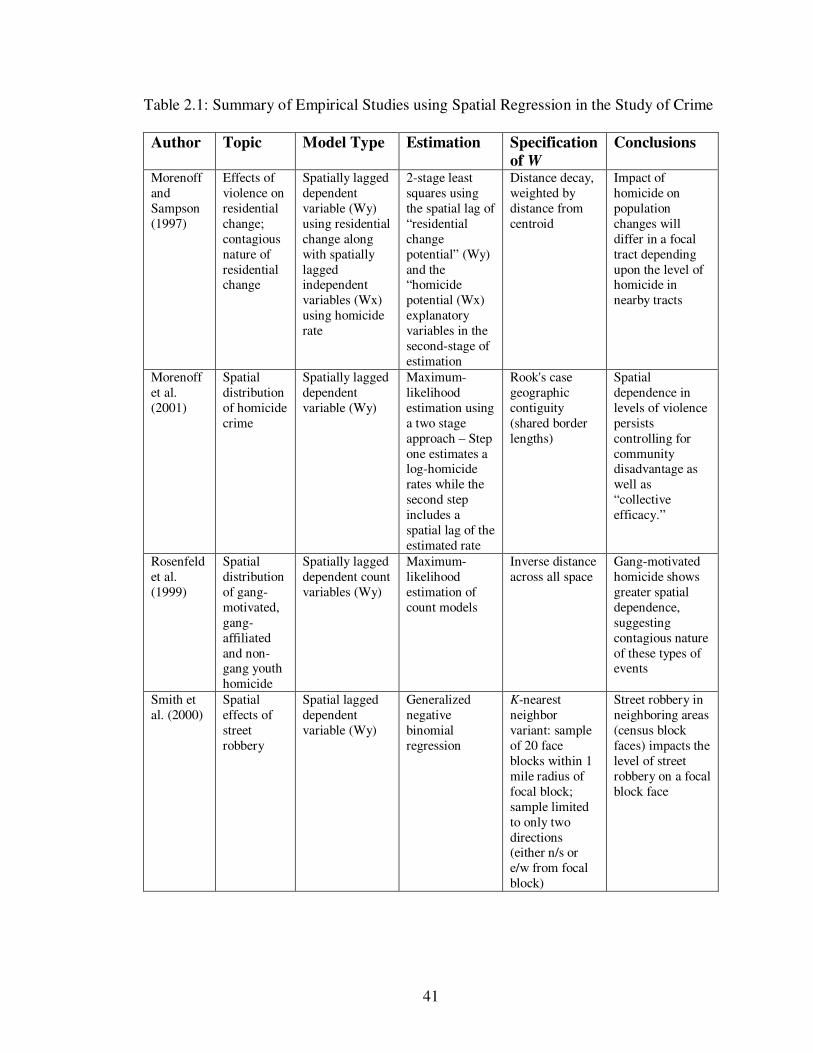
41

Table 2.1: Summary of Empirical Studies using Spatial Regression in the Study of Crime

Author Topic Model Type Estimation Specification

of W

Conclusions

Morenoff and Sampson (1997)

Effects of violence on residential change; contagious nature of residential change

Spatially lagged dependent variable (Wy) using residential change along with spatially lagged independent variables (Wx) using homicide rate

2-stage least squares using the spatial lag of “residential change potential” (Wy) and the “homicide potential (Wx) explanatory variables in the second-stage of estimation

Distance decay, weighted by distance from centroid

Impact of homicide on population changes will differ in a focal tract depending upon the level of homicide in nearby tracts

Morenoff et al. (2001)

Spatial distribution of homicide crime

Spatially lagged dependent variable (Wy)

Maximum-likelihood estimation using a two stage approach – Step one estimates a log-homicide rates while the second step includes a spatial lag of the estimated rate

Rook's case geographic contiguity (shared border lengths)

Spatial dependence in levels of violence persists controlling for community disadvantage as well as “collective efficacy.”

Rosenfeld et al. (1999)

Spatial distribution of gang-motivated, gang-affiliated and non-gang youth homicide

Spatially lagged dependent count variables (Wy)

Maximum-likelihood estimation of count models

Inverse distance across all space

Gang-motivated homicide shows greater spatial dependence, suggesting contagious nature of these types of events

Smith et al. (2000)

Spatial effects of street robbery

Spatial lagged dependent variable (Wy)

Generalized negative binomial regression

K-nearest neighbor variant: sample of 20 face blocks within 1 mile radius of focal block; sample limited to only two directions (either n/s or e/w from focal block)

Street robbery in neighboring areas (census block faces) impacts the level of street robbery on a focal block face

42

Table 2.1: Continued

Author Topic Model Type Estimation Specification

of W

Conclusions

Baller et al. (2001)

County level spatial patterns of homicide

Spatial regimes; Spatial error and spatially lagged dependent variable (Wy; We)

Maximum-likelihood: Robust Lagrange Multiplier tests

K-nearest neighbor (all counties connected to exactly 10 nearest (by centroid distance) neighboring counties)

South US region shows evidence of homicide diffusion; spatial dependence in non-South likely due to unobserved variables

Gorman et al. (2001)

Effects of alcohol outlets on violent crime rates

Spatial error and spatially lagged independent variables (Wx, We)

Maximum likelihood

Queen’s case geographic contiguity (shared border lengths and/or border points)

The density of alcohol outlets in neighboring areas had no significant impact on crime rates in focal units.

Mears and Bhati (2006)

Spatial distribution of homicide, by type

Spatially lagged dependent variable (Wy); Socially lagged dependent variable; Social and spatially weighted independent variables (Wx).

Negative Binomial using natural log of homicide counts

Geographic space is measured using queen’s case contiguity; Social space is measured by comparing measures of social similarity (including resource deprivation) between each pair of communities. The similarity matrix decays exponentially as dissimilarity increases.

With the exception of gang homicide, social similarity among geographic units is more strongly related to homicide than is geographic adjacency.

Kubrin and Stewart (2006)

Effects of neighborhood context on recidivism rates

Multi-level model (included a spatial lag variable) (Wy)

HLM with the inclusion of a spatially lagged measure of recidivism rates.

Queen’s case geographic contiguity

Spatial dependence in recidivism; unable to assess evidence for diffusion

43

Table 2.1: Continued

Author Topic Model Type Estimation Specification

of W

Conclusions

Tita (2006); Tita and Greenbaum (2009)

Spatial distribution of Gang violence

Spatially lagged dependent variable (Wy); Socially lagged dependent variable

“Anselin-alternative Method” using the “violence potential” as an instrumental variable in 2-stage estimation

Geographic space is measured using queen’s case contiguity; Social space is constructed using the location of gangs in space, and the rivalry network that links them socially

Spatial dependence is best modeled by considering the socio-spatial distribution of gang rivalries, which extend beyond contiguous neighbors.

Hipp et al. (2009)

Intra-group and Inter-group Violence

Spatially lagged independent variables (Wx)

Negative Binomial with spatially lagged X’s

Distance decay, 2 mile maximum

Clear evidence of income inequality and racial transition in surrounding tracts impacting inter-group violence in focal tract

44

Figure 2.1: Spatial data may demonstrate a pattern of positive spatial autocorrelation (left), negative spatial autocorrelation (right), or a pattern that is not spatially autocorrelated (center). Statistical tests, such as Moran’s I, should always be used to evaluate the presence of spatial autocorrelation.

45

CHAPTER 3

THEORIZING SPACE AND PLACE FOR SPATIAL

ANALYSIS IN CRIMINOLOGY

This chapter is drawn from a conceptual essay published in a special issue of the

Journal of Quantitative Criminology (Tita and Radil 2010a) and presents a theoretical

framework for understanding and modeling context that builds on the place concept in

geography that emphasizes connections between places. Therefore this essay may be seen

as akin to a theory chapter in a traditional dissertation format and is offered in that spirit.

It is presented here in a slightly altered form from Tita and Radil (2010a) to avoid

duplication with the previous chapter.

INTRODUCTION

In this essay, we attempt to better understand the role that place plays in

explaining the spatial distribution of crime. We briefly explore the relevant

criminological literature beginning with the works published in the last decade and

comment on the important contributions and advances achieved since then. Though a

formal review of the voluminous literature even on this subset of spatial analysis is far

beyond the scope of this paper, we do try to highlight some of the more seminal findings

along with more recent works that employ innovative approaches to understanding the

spatial distribution of crime. In terms of advancing the field of spatial analysis, we focus

on two important issues that are beginning to garner increasing attention within the crime

literature: Defining and measuring “place” and the adoption of more deductive models

that attempt to capture particular processes of influence in the specification of the spatial

weights matrix, represented as W.

46

Clearly the development of important theoretical constructs related to the ecology

of crime far pre-date the availability of user-friendly, off-the-shelf mapping and spatial

analysis software. However, it would be very difficult to overstate the important role

these tools played over the last decade in terms of advancing our understanding of the

spatial distribution of crime. The mapping of crime incident data permits one to explore

how the built environment, the presence of certain types of businesses or activities, or

characteristics of the local residential population impact the observed spatial distribution

of crimes. The impact of bars, public housing or illicit activities such as gangs or drug

markets on local patterns of crime has been of particular interest (Tita and Ridgeway

2007; Taniguchi et al. 2011). One can also determine how the spatial distribution of

crime changes over different time scales. For instance, in the short term, one might be

interested in determining how the policing of drug markets or gang areas might impact

the spatial distribution of crime (e.g., Braga 2001; Tita et al. 2003). In fact, using GIS and

spatial analysis in the evaluation of such place-based policing strategies has resulted in

the robust conclusion that crime does not “move around the corner” and that rather than a

displacement effect, we often see a diffusion of the benefits of place-based policing to

adjoining areas (Bowers and Johnson 2003; Weisburd et al. 2006). One can also look

over longer time periods, and at larger units of analysis, to examine the relationship

between changes in the socio-economic composition of local neighborhoods and the

spatial distribution of crime (Cullen and Levitt 1997; Morenoff and Samspon 1997; Hipp

et al. 2009).

It is worth noting that the term “spatial analysis” applies equally to the study of

incident level point patterns (e.g., crime hot spots) as well as to the study of aggregated

47

crime counts or rates at the area level (e.g., spatial autocorrelation among census block

groups, tracts, or “neighborhoods”). For our purposes, we focus solely on the spatial

analysis of crime at the aggregate rather than the incident level.10

ECOLOGICAL STUDIES OF CRIME – THE USE OF SPATIAL REGRESSION

MODELS

In a review of the growing use of spatial approaches in criminology, Cohen and

Tita (1999a) noted that the growing spatial analysis of crime literature was enabling

criminologists to move beyond simply mapping crime and demonstrating that crime does

indeed cluster in space. Indeed many studies over the last two decades have begun to

seriously consider why crime clustered in space and search for evidence of diffusion

across space (e.g., Morenoff and Sampson 1997). In the time since Cohen and Tita

(1999a), spatial regression models were often used in an attempt to construct, inductively,

explanation for the observed patterns of spatial clusters. In addition to crime, researchers

began to use spatial regression models to demonstrate that many negative health issues

including, but not limited to, low birth weight (Morenoff 2003), infant mortality (Rushton

et al., 1996), and depression (Ross 2000) also cluster spatially (for a complete review of

the neighborhood effects literature see Sampson et al., 2002). From these studies

emerged a consistent set of explanatory variables that characterize “bad” neighborhoods

(e.g., concentrated poverty, stability of residents, female headed households, minority

10 We would be remiss if we did not mention two areas of growing importance. Trajectory models are being employed by a number of researchers to examine the “criminal careers” of communities (Weisburd et al. 2004; Groff et al. 2009). Griffiths and Chavez (2004) used this method to focus specifically on the issue of diffusion. Second, there have been two recent publications within the criminology literature (Cahill and Culligan 2007; Graif and Sampson 2009) that argue for the primacy of Geographically Weighted Regression (GWR) over “global” regression models. GWR differs in that it does not assume stationarity, thus coefficients are permitted to vary over different regions of one’s study area.

48

population), and that there appeared to be an aggregate effect, dubbed a “neighborhood

effect,” to living in these places. For instance, concentrated poverty negatively impacts

all residents of a community regardless of one’s own level of personnel income. That

such places also cluster in space suggests that neighborhoods are not independent units of

observation. On one hand the lack of independence might simply be a result of the

clustering of important variables such as race and poverty in space. On the other hand, it

was posited that there might be forces at work that make the level of crime in one

neighborhood dependent upon the actions and activities occurring in other areas

(Sampson 2004; Morenoff et al. 2001). That is, social processes might be at work that

result in the diffusion, or contagion of crime, across space over time (for a discussion of

the types of diffusion and contagion, see Cohen and Tita 1999).

In trying to further understand the patterns and the spread of violence, spatial

regression (or spatial econometrics) quickly became, and remains, the methodology of

choice. As noted above, spatial autocorrelation occurs when the values of variables

sampled at nearby locations are not independent from each other. This lack of

independence makes the use of OLS regression techniques inappropriate. While there are

a variety of methods to address spatially autocorrelated data, simultaneous autoregressive

(SAR) models have become the most popular, especially spatial error models and spatial

lag (or “dependence”) models (see Tita and Radil 2010a).

Spatial error models are appropriate for modeling unobservable processes (e.g.,

norms or beliefs) that are shared among individuals residing in proximate places, or when

the boundaries that separate “places” are arbitrary to the extent that two “different” places

49

are actually very similar across various social, economic, or demographic features (i.e.,

the clustering of like places). The spatial error models takes the following form:

,with , ; I =] uE[u 0, =E[u] u + = + X = Y 2σλεεεβ ′

where ε = Wε, and W is the (N x N) autocorrelation weighting matrix that contains

information about which spatial units (e.g., census tracts, neighborhoods) are spatially

connected and λ measures the spatial correlation of the error term. In the absence of

correlation among neighbors' error terms, the λ equals zero therefore using OLS methods

is appropriate. Failure to account for the non-dependence in the error will still yield

unbiased coefficients; however, estimates of the standard errors on those coefficients will

be incorrect (Anselin 2002).

When the level of crime in one neighborhood is directly dependent upon the

activities or social processes occurring in a neighboring area, one must apply a spatial lag

(spatial dependence) model. Failure to consider spatial dependence in one’s model is far

more serious than ignoring spatially autocorrelated error terms because the model is mis-

specified and the estimates of the coefficients are incorrect. The spatial lag model takes

the form:

, with, I =] E[ 0, =] E[ + X + WY = Y 2σεεεεβρ ′

where ρ is the spatial coefficient on the spatially lagged dependent variable, and it will be

nonzero if outcomes in one location influence outcomes in another location. W is once

again the (N x N) autocorrelation weighting matrix.

The autocorrelation matrix, W, is what adds a spatial dimension to the above

models allowing the researcher to define which spatial units are related. Though formal

statistical models of spatial autocorrelation are relatively new, most crime researchers

50

continue to rely on the specification of one’s spatial weights matrix, W, using either

spatial contiguity/adjacency or by employing measures of distance decay. The decision to

employ such measures is consistent with Tobler’s First Law of Geography (Tobler 1970),

which states that “Everything is related to everything else, but near things are more

related than distant things.” Our goal is not to refute this assertion or criticize studies that

continue to rely on weights matrices specified in this manner. In fact, there are plenty of

theories to support the notion that crime in a focal area influences the amount of crime in

immediately proximate areas and in such cases, this is the correct specification of how

space matters in W. However, we do want to highlight innovative attempts to model

crime by recognizing that crime in a focal area may directly influence crime in

geographically distant areas.

As we have noted elsewhere (Tita and Greenbaum 2009; Tita and Radil 2010b),

the selection of which model, error or lag, has, and continues to be, driven by conducting

goodness of fit tests rather than theory. Similarly, in the case of the estimate of spatial

lag models, the conventional approach has been inductive by nature as post-hoc

explanations of why “space matters” are constructed after the models are estimated.

Again, as with the specification of W by only considering strictly geographic notions of

space, we do not want to be overly critical. Empirical exercises to choose one’s model

and inductive reasoning have added tremendously to the collective understanding of the

diffusion of violence. However, as Radil et al. (2010) cautions, it is important to remain

vigilant against a sort of “spatial fetishism” in which the ability to simply map crime

patterns takes precedence over attempting to explain the causes of the clusters. That is,

“When spatial analysis is overly dependent on reasoning from spatial form to social

51

process, the risk of reducing people to the spaces they occupy grows while the likelihood

of new insights shrinks” (Radil et al. 2010: 308).

As noted above, the theme of diffusion for the Special Issue was motivated by the

unprecedented growth in levels of youth homicide during the late 1980s through the early

1990s. As a result, criminologists began to adopt an epidemiological framework and

speak of the contagious diffusion of violence. The simple descriptive analysis of

homicide data showed that urban minority males killed with guns represented the

subpopulation at greatest risk for victimization. The combination of exploratory spatial

data analysis and spatial regression analysis found evidence in support of the conclusion

that violence was diffusing at the national level (Blumstein and Rosenfeld 1998; Cork

1999; Kellerman 1996), county level (Messner et al. 1999; Baller et al. 2001; Messner

and Anselin 2004), and local levels (Block and Block 1993; Cohen and Tita 1999; Fagan

et al. 1998; Kennedy and Braga 1998; Klein et al. 1991; Morenoff et al. 2001).

As we have noted elsewhere (Tita and Radil 2010b), these early studies were

important because they began to hint at the structures and underpinnings of social

processes that might help us understand why violence diffuses across space.

Collectively, these studies also found that the clustering of violence is better explained

using spatial lag models (i.e., the result of an unobserved pattern) rather than spatial error

models (i.e., the result of the clustering of covariates). By examining the statistically

significant coefficient on the spatially lagged dependent variable, specific explanations

were offered regarding the forces driving the spread of lethal violence within urban

settings. Most frequently, the explanations offered in the above studies included some

(or all) elements of the proliferation of crack cocaine markets, an increase in the carrying

52

and use of guns by youths, and/or the emergence of urban street gangs. More recently, the

impact of parolees re-entering communities on crime (and recidivism) has been examined

(Kubrin and Stewart 2006).

DEDUCTIVE SPATIAL MODELS AND ALTERNATIVE MEASURES OF “SPACE”

There have been several novel attempts to capture the geographic dimensions of

the forces that influence the spread of violence by offering alternative specifications of

the autocorrelation matrix. These new techniques take a deductive approach to the

modeling of specific social processes believed to be driving the diffusion of crime and are

based in the “social influence” literature wherein social network analysis has been used to

understand the diffusion/adoption of norms or innovations among individuals or

organizations (see Marsden and Friedkin 1994; Leenders 2002).

In one of the first attempts to geographically “unbound” the autocorrelation

matrix, Mears and Bhati (2006) model homicide by exploiting the finding that social

similarity increases the probability of communication and social interaction (see

McPherson et al. 2001). The researchers examined race, ethnicity and income at the tract

level and linked together the tracts only if the residents were similar. They argue that

events in a focal area will be influenced more strongly by events in non-adjacent but

socially similar areas than in adjacent, but socially dissimilar areas. The authors find

support for this argument and conclude that social distance is important. However, space

also matters and the influence of violence in one area has on violence in another is

especially powerful when the areas are both spatially and socially proximate.

53

Tita and Greenbaum (2009) and Tita and Radil (2011) provide examples of how

the spatial and social dimensions of urban street gangs can be exploited in an inductive

approach. Their research argues that gangs are likely to be especially relevant to diffusion

because they are organizations that are sustained over time through continuing social

interactions within specific geographic locations and because the area in which gangs

hang out experience high levels of crime, especially violence (Kennedy et al. 1997; Tita

and Ridgeway 2007.) Their inductive models of violence exploit social network data on

gang rivalries along with the location of gang “set space” (Tita et al. 2005). Using matrix

algebra, an autocorrelation matrix (W) is constructed wherein a non-zero value indicates

that a pair of geographic units contains the set space of rival gangs. The results from

studies in Pittsburgh and Los Angeles were consistent in demonstrating that the weights

matrix that considers the socio-spatial nature of gangs and their rivalries provides a better

fit to the data.

Different types of violence/crime will require different theories and different

specifications of the spatial autocorrelation matrix. For instance, one might model the

diffusion of youth violence by considering social interactions that occur within schools.

In such a case neighborhoods would be linked together if and only if they send students

to the same school buildings. Though Meares and Bhati (2006) have strong theoretical

justification for modeling patterns of influence using measures of similarity, studies that

capture the social networks and communication networks would provide an empirical

validation of their approach. In fact, a recent publication in the journal Science provides

an excellent template for how such a study could be accomplished.

54

Interested in testing the relationship between community level economic

development (employment) and interpersonal social networks, Eagle et al. (2010), are

able to measure the patterns of social interactions for the entirety of the United Kingdom.

Each year in August, the “from” and “to” locations for over 99 percent of the land line

telephone calls and over 90 percent of all cell phone calls are recorded. The researchers

used this dataset to test the “strength of weak ties” argument (Granovetter 1973) by

examining the level of social, economic and demographic (dis)similarity between the

locations of the communicating parties. Their analysis demonstrates that communities

that place calls to others who reside in places heterogeneous from their own fare much

better economically.

One could imagine using geographically identified communication data for a

variety of reasons within the community and crime literature, in general, in the spatial

analysis, in particular. As used in the original article, the communication patterns could

be used to construct community-level measures of “bridging” versus “bonding” social

capital (see Tita and Boessen forthcoming). It could also be used in the construction of

spatial autocorrelation matrices. One could create a simple binary matrix in which two

areas were identified as “neighbors” if the number of calls linking the two areas exceeded

a user set threshold. Measuring the frequency of calls between two areas would permit

one to capture the strength of the link between the two communities, though this would

be complicated by mobile phone technology. Using this information would result in a

correlation matrix that explicitly includes a weighted measure of the potential for

activities in one area to influence crime in another based not on geography, but on the

social distance between places.

55

DEFINING PLACE FOR SPATIAL ANALYSIS

As noted above, spatial approaches in criminology have a long history of drawing

upon geographic concepts, and later, geographic technologies. One particular way in

which geographers and criminologists have tried to understand the behavior of social

actors is through the concept of place. Place is one of the most central concepts in

geography (e.g., Relph 1976; Tuan 1977; Entrinkin 1991; Sack 1997; Staehel, 2003;

Cresswell 2004) and a great deal of research in spatial criminology makes use of different

aspects of the place concept, albeit sometimes uncritically. As such, we begin with a

discussion of the place concept, how it is used in different research traditions in

geography, and how such approaches can inform current and future research in

criminology.

Place seems simple enough on the surface but a great many scholars have

struggled to describe and define exactly what is place. As noted by Staeheli (2003),

Cresswell (2004) and others, place is a multifaceted concept and often used in different

ways within different research traditions. For example, Staeheli (2003: 159) identifies

different but interrelated perspectives on place within geography: place as a physical

location or site; as a cultural and/or social location; as context; as something socially

constructed over time; and as an ongoing process. These various elements and

perspectives on place should be read as fundamentally interrelated although some are

more prominent than others. For example, nearly all contemporary work explicitly

involving place in human geography proceeds from assuming that places are socially

constructed and are the products of human activity. From this starting point, the research

56

questions involving place range from ideographic approaches that emphasize the

distinctiveness of a given place to those that attempt to explain such uniqueness by

reference to wider political or economic processes or structural conditions (Cresswell

2004).

As noted by Staeheli (2003), understanding place as a specific physical location

or an otherwise bounded site is a common approach, especially within spatial analytic

traditions in geography. Expressly spatial approaches are often framed as the study of

relationships that connect discrete places (e.g., Staeheli 2003). In other words, in this

tradition, places are typically seen as discrete locations in a spatial setting. However, this

tradition also deemphasizes the uniqueness or distinctiveness of places and a

consideration of place becomes a question of research design: how to select observation

locations or sites for research. Places then are defined primarily spatially. The issues

focus on how locations are bounded in space, how distant sites are from each other on a

spatial plane, etc.

Another approach to place familiar to the ecological tradition in criminology is to

see place as context. This approach also has been important in many different subfields of

geography and tends to see places as part of a broader environmental context which one

must consider to fully understand human action (which of course occurs within 'places',

i.e. specific locations). The characteristics of places are typically understood as potential

'variables' for a statistical/spatial analysis in this approach in geography, criminology, and

many other fields of study (see O’Loughlin 2000, 2003). The place as context approach is

neither new nor exclusive to geography (see for example Émile Durkheim's (1897)

research on the environmental and personal factors associated with suicide). However,

57

understanding place as context tells one little about the appropriate way in which to

define a place or a series of places for systematic study.

These two perspectives on place are at the heart of an emerging technical

discussion in criminology about the importance of considering the proper level of

aggregation when estimating neighborhood effects for spatial modeling (see Hipp 2007;

Wiesburd et al. 2008; Wiesburg and Braga 2010). As Hipp (2007) points out, in the

ecological tradition in criminology, data is typically aggregated to geographic areas

which vary in size and configuration, such as census units, which typically serve as the

units of analysis for spatial models. Taking this approach to the study of crime leaves one

confronted with the challenges of the modifiable areal unit problem, or MAUP

(Openshaw and Taylor 1979, 1981; Openshaw 1984; see Gehlke and Beh, 1934 or

Robinson 1950 for classic examples of MAUP, or Openshaw 1996 for a more

contemporary review). The modifiable areal unit problem arises from the fact that areal

units are usually arbitrarily determined in the sense that they can be aggregated or

disaggregated to form units of different sizes or spatial arrangements (in other words,

they are ‘modifiable’). MAUP involves two interrelated elements, the scale problem and

the zoning problem (Openshaw and Taylor 1979). Openshaw and Taylor (1979: 128)

describe the scale problem as “the variation in results that may be obtained when the

same areal data are combined into sets of increasingly larger areal units of analysis,” and

the zoning problem as “variations in results due to alternative units of analysis where n,

the number of units, is constant.” For the scale problem, increasing the aggregation of

units by increasing the area covered by the units (which also typically involves

decreasing the total number of units for a given area) decreases the variance in the data

58

between the units. For the zoning problem, rezoning the areas contained by each unit

while holding the total number of units the same can impact both the mean and variance

of any measured data.

These issues have important implications for ecological studies of crime as

multivariate statistical analyses can be sensitive to variations in scale and zoning systems,

leading to highly unreliable results (e.g., Fotheringham and Wong 1991). The problems

posed for statistical inference from MAUP have led some to conclude that all methods

whose results depend on areal units should be discarded and techniques independent of

areal units should be used (e.g., Tobler 1989; see also Openshaw and Taylor 1981;

Openshaw 1984; Fotheringham 1989; Fotheringham and Wong 1991; Fotheringham and

Rogerson 1993). Grid-based models have also been advocated in spatial analysis to avoid

the use of inconsistently sized areal units but the issues of the choice of grid size and the

associated level of aggregated information remains. Hipp’s advice is not as extreme as

Tobler’s (1989), but he does advocate that analysts should carefully consider whether a

particular geographic unit of analysis “is actually appropriate for the outcome of interest

or the structural predictors being used” (2007: 660). Given that there remains no technical

solution to the problems posed by MAUP, Hipp’s (2007) advocacy for theory to guide

one’s choice of the appropriate spatial unit of analysis is crucial.

In response to a growing recognition of the need for a careful consideration of the

concept of place and of how place can be operationalized for the systematic study of

crime, Hipp (2007) argues for a move toward using geographically smaller units of

analysis and, correspondingly, less aggregated data in the spatial analysis of crime (see

also Hipp et al. 2009). For example, Hipp (2010) describes a unit of analysis for spatial

59

modeling that he calls “micro-neighborhoods” which consist of around 10 households.

The obvious size reference (“micro”) in Hipp’s (2010) unit of analysis suggests the utility

of another geographic concept, that of scale, when considering the question of defining

and operationalizing place for systematic analysis. Scale, which refers to the geographic

scope or reach of a given phenomena (see Marston et al. 2005), is necessary to consider

when attempting to specify any geographically-based unit of analysis. In other words,

scale is implicated in thinking about how places are bounded in space. However, scale

has also been heavily critiqued in recent debates in human geography about the nature of

the concept and its utility in geographic research (e.g., Herod and Wright 2002;

Mamadouh et al. 2004; McMaster and Sheppard 2004; Marston et al. 2005)

The arguments about scale focus on the geographic reach and scope of the social

activities that are presumed to form places and how such scales can be and are routinely

created, maintained, and marshaled by people for certain political and economic agendas

(e.g., Taylor 1982; Smith 1992; Swyngedouw 2004). An important element of these

critiques for this discussion is that the larger the scale that one chooses to focus upon to

define a place or to otherwise bound or delimit a place, the more likely it is that the

specific issue of interest can be obscured from the analyst by processes operating at

various other scales and in various other places (e.g., Massey 1997). The broad point for

criminology from these debates is that analysts should be ever cautious of uncritically

using arbitrary or pre-given units for analysis or of assuming that such units can or should

be thought of as ‘places’. The reference to micro-scale units in criminology research

(e.g., Hipp 2010) evokes this point and the scale/place debates in geography help draw

attention toward careful and theoretically informed thinking of about places.

60

The move toward smaller scale units of analysis can be seen as perhaps driven by

the technical issues of data collection and levels or aggregation (e.g., MAUP) but should

also be one in which the insights of the scale/place debates are considered. A careful read

of the technical and theoretical issues involved with delimiting space for systematic study

makes it clear that it is “geographical scale that defines the boundaries and bounds the

identities around which control is exerted and contested” (Smith, 1992: 66). In short, the

scales used to delimit places that could be used as units of analysis are products of myriad

human action and goals. Places, therefore, are never natural, preformed, or given and

there is no such thing as the ‘right’ scale for any given research topic or interest. Hipp

(2007, 2010), Hipp et al. (2009), and others are to be commended for suggesting

approaches that consciously attempt to deal with the challenges posed by MAUP. But just

as with grid-based approaches, the ‘smaller is better’ micro-scale approach to place in

criminology must still wrestle with the problems of place as something that is ultimately

socially constructed and therefore contested and subject to change as well as with the

perhaps more familiar technical issues of MAUP.

Given the combination of the realities of the high costs of collecting data and the

general availability of census data, it is unlikely and perhaps unreasonable to expect that

criminologists will abandon the use of geographic units with some amount of aggregated

data (such as census units). Accordingly, there are some innovative advances being

undertaken which rely upon capturing the spatial dimension of social networks to define

the geography of a community.11 For example, Radil et al. (2010) and Tita and Radil

11 A move toward using social networks (either empirically or conceptually) is also evident in geography where concerns about the problems with scale have led some to turn to network models of social process (notable examples from a variety of geographic sub-disciplines include Cox 1998; Amin 2002; and Flint et al. 2009).

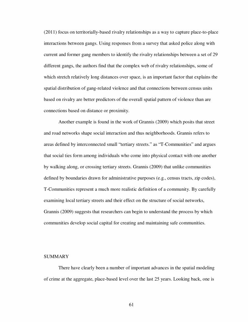
61

(2011) focus on territorially-based rivalry relationships as a way to capture place-to-place

interactions between gangs. Using responses from a survey that asked police along with

current and former gang members to identify the rivalry relationships between a set of 29

different gangs, the authors find that the complex web of rivalry relationships, some of

which stretch relatively long distances over space, is an important factor that explains the

spatial distribution of gang-related violence and that connections between census units

based on rivalry are better predictors of the overall spatial pattern of violence than are

connections based on distance or proximity.

Another example is found in the work of Grannis (2009) which posits that street

and road networks shape social interaction and thus neighborhoods. Grannis refers to

areas defined by interconnected small “tertiary streets.” as “T-Communities” and argues

that social ties form among individuals who come into physical contact with one another

by walking along, or crossing tertiary streets. Grannis (2009) that unlike communities

defined by boundaries drawn for administrative purposes (e.g., census tracts, zip codes),

T-Communities represent a much more realistic definition of a community. By carefully

examining local tertiary streets and their effect on the structure of social networks,

Grannis (2009) suggests that researchers can begin to understand the process by which

communities develop social capital for creating and maintaining safe communities.

SUMMARY

There have clearly been a number of important advances in the spatial modeling

of crime at the aggregate, place-based level over the last 25 years. Looking back, one is

62

hard pressed to even identify the existence of expressly spatial analytic approaches to

understanding crime until the concurrent development of and widespread access to both

desktop mapping and spatial statistical software in the early to mid-1990s (e.g., desktop

GIS packages and spatial software such as SpaceStat). It is clear that we have come very

far in a relatively short period of time. In fact, we've come so far that it is now difficult to

argue that the most pressing needs for the future of the spatial analysis of crime are either

technological or methodological in nature. It is our conclusion that the most pressing

issues remain to do with the sound theorization of human behavior and crime in

geographic space and with making sure that the now sophisticated spatial methods that

we do use are those that flow from and are informed by theory.

As it turns out, this is an old dilemma for spatial analysis. For example, it was

more than 30 years ago that geographer Piers Blaikie (1978: 276) took stock of the state

of affairs of diffusion research in geography and remarked that the application of

sophisticated quantitative spatial techniques “has been more concerned with the

techniques themselves than what they tell us about the process of spatial diffusion. The

preoccupation with spatial form without an adequate theory of process has meant that the

progress in technique has not been able to help progress in theory.” Blaikie (1978: 276)

concluded that methods should be a secondary concern “until a satisfactory theoretical

framework [for diffusion] is devised.” Unfortunately, things may not have changed as

much as we would hope. Arthur Getis, a foundational figure in spatial analysis, recently

argued that overly simplistic notions of the importance of distance to human activity

(which he traces to 19th century 'least effort' theories of human activity; see also Isard

(1956)) continue to underpin most spatial modeling research and that “unfortunately for

63

the discipline of geography, no substantial work about distance theory has occurred since

the 1960s and early 1970s” (Getis 2009: 407).

From these perspectives, the challenges for future work are not those that pertain

to the development of new mapping technologies or more sophisticated statistical

methodologies (e.g., geographically weighted regression, the development of Bayesian

methods in spatial analysis). The most pressing issues remain connected to the sound

theorization of spatial human behavior. The most important developments have, and

continue to occur, within the realm of theory and good science. That is, regardless of how

sophisticated our methodologies become for the estimation of spatial models, the key will

always be that the specification of these models be sound in terms of the measurement

and definition of place and the manner in which areas are deemed “neighbors.”

In using spatial regression methods to explain crime patterns, we are respectful

that researchers relying on official sources of data such as the Census Bureau will forever

be hamstrung by the availability of meaningful covariates that are aggregated to the

appropriate level of crime. Being mindful that place is often socially constructed and that

various criminological theories suggest social processes that operate at different spatial

resolution is all the more important. It is also vital that, in the case of spatial lag models,

one must carefully consider the full geographic extent in which the events in one area can

influence events in other areas regardless of the geographic distance between them.

Though the influence for a crime in a focal area in other areas might decay over distance,

it is possible that there are other networks of social interactions (e.g., interactions that

occur outside the neighborhood at work or school, participation in voluntary or religious

organizations, adversarial networks as presented in our gang example) that make events

64

in one area extremely salient in the commission of future events in otherwise

geographically distant areas.

65

CHAPTER 4

MODELING SOCIAL PROCESS IN THE

SPATIAL WEIGHTS MATRIX

This chapter, published in the Journal of Quantitative Criminology (Tita and

Radil 2011), examines alternative specifications of the spatial weights matrix and

compares more common distance-based (adjacency-based) specifications with those that

are more explicitly grounded in a theory of competition between the gangs. These

alternative specifications are used in spatial regression models and the impact of the

different specifications on model performance is evaluated. An important finding from

this chapter is that a ‘hybrid’ spatial weights matrix can be constructed that captures both

distance-based and social relationship-based interactions. This finding leads directly to

the research presented in the next chapter. This paper is presented in this chapter

unaltered from the published version aside from minor formatting changes.

INTRODUCTION

Social networks are often implicated as being important mechanisms in the

development and maintenance of safe, low crime neighborhoods (e.g., Taylor et al. 1984;

Sampson 1988; Sampson et al. 1997; Veysey and Messner 1999; Bellair 2000). The

research on the relative importance of local, as well as non-local, social ties is framed

within either the systemic model of social disorganization (e.g., Shaw and McKay 1942;

Sampson 1986; Sampson and Groves 1989; Bursik and Grasmick 1993) or the more

recent conceptual framework of “collective efficacy” (Sampson et al. 1997; Sampson

2004). In either case, these approaches argue that it is the individual-level social bonds

among local residents that facilitate the formation of informal social control and the

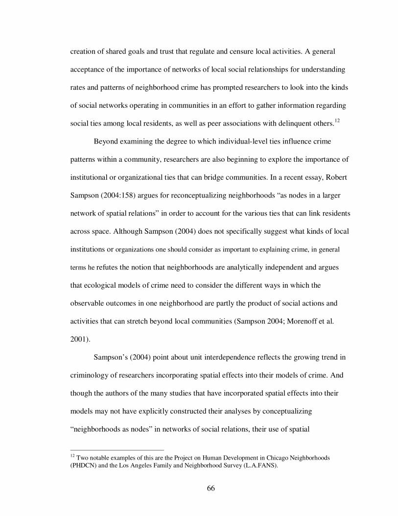
66

creation of shared goals and trust that regulate and censure local activities. A general

acceptance of the importance of networks of local social relationships for understanding

rates and patterns of neighborhood crime has prompted researchers to look into the kinds

of social networks operating in communities in an effort to gather information regarding

social ties among local residents, as well as peer associations with delinquent others.12

Beyond examining the degree to which individual-level ties influence crime

patterns within a community, researchers are also beginning to explore the importance of

institutional or organizational ties that can bridge communities. In a recent essay, Robert

Sampson (2004:158) argues for reconceptualizing neighborhoods “as nodes in a larger

network of spatial relations” in order to account for the various ties that can link residents

across space. Although Sampson (2004) does not specifically suggest what kinds of local

institutions or organizations one should consider as important to explaining crime, in general

terms he refutes the notion that neighborhoods are analytically independent and argues

that ecological models of crime need to consider the different ways in which the

observable outcomes in one neighborhood are partly the product of social actions and

activities that can stretch beyond local communities (Sampson 2004; Morenoff et al.

2001).

Sampson’s (2004) point about unit interdependence reflects the growing trend in

criminology of researchers incorporating spatial effects into their models of crime. And

though the authors of the many studies that have incorporated spatial effects into their

models may not have explicitly constructed their analyses by conceptualizing

“neighborhoods as nodes” in networks of social relations, their use of spatial

12 Two notable examples of this are the Project on Human Development in Chicago Neighborhoods (PHDCN) and the Los Angeles Family and Neighborhood Survey (L.A.FANS).

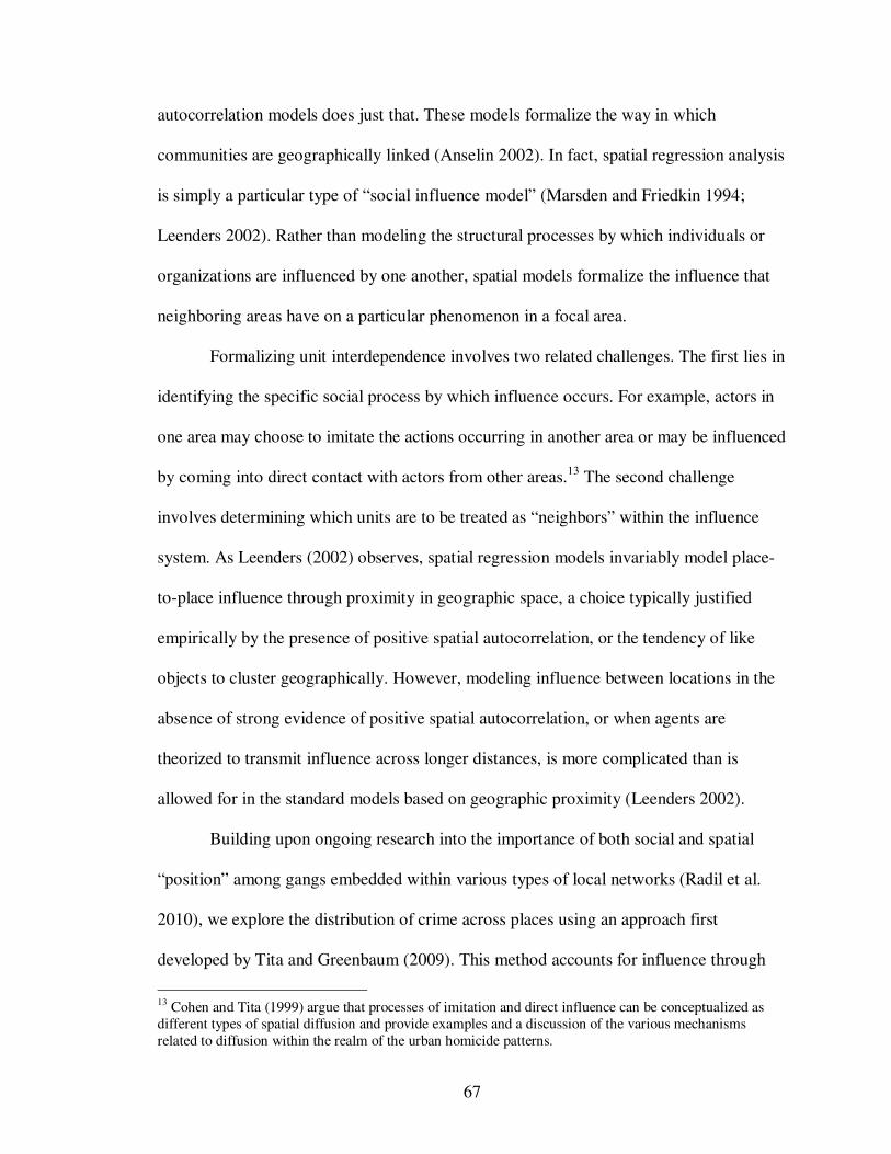
67

autocorrelation models does just that. These models formalize the way in which

communities are geographically linked (Anselin 2002). In fact, spatial regression analysis

is simply a particular type of “social influence model” (Marsden and Friedkin 1994;

Leenders 2002). Rather than modeling the structural processes by which individuals or

organizations are influenced by one another, spatial models formalize the influence that

neighboring areas have on a particular phenomenon in a focal area.

Formalizing unit interdependence involves two related challenges. The first lies in

identifying the specific social process by which influence occurs. For example, actors in

one area may choose to imitate the actions occurring in another area or may be influenced

by coming into direct contact with actors from other areas.13 The second challenge

involves determining which units are to be treated as “neighbors” within the influence

system. As Leenders (2002) observes, spatial regression models invariably model place-

to-place influence through proximity in geographic space, a choice typically justified

empirically by the presence of positive spatial autocorrelation, or the tendency of like

objects to cluster geographically. However, modeling influence between locations in the

absence of strong evidence of positive spatial autocorrelation, or when agents are

theorized to transmit influence across longer distances, is more complicated than is

allowed for in the standard models based on geographic proximity (Leenders 2002).

Building upon ongoing research into the importance of both social and spatial

“position” among gangs embedded within various types of local networks (Radil et al.

2010), we explore the distribution of crime across places using an approach first

developed by Tita and Greenbaum (2009). This method accounts for influence through

13 Cohen and Tita (1999) argue that processes of imitation and direct influence can be conceptualized as different types of spatial diffusion and provide examples and a discussion of the various mechanisms related to diffusion within the realm of the urban homicide patterns.

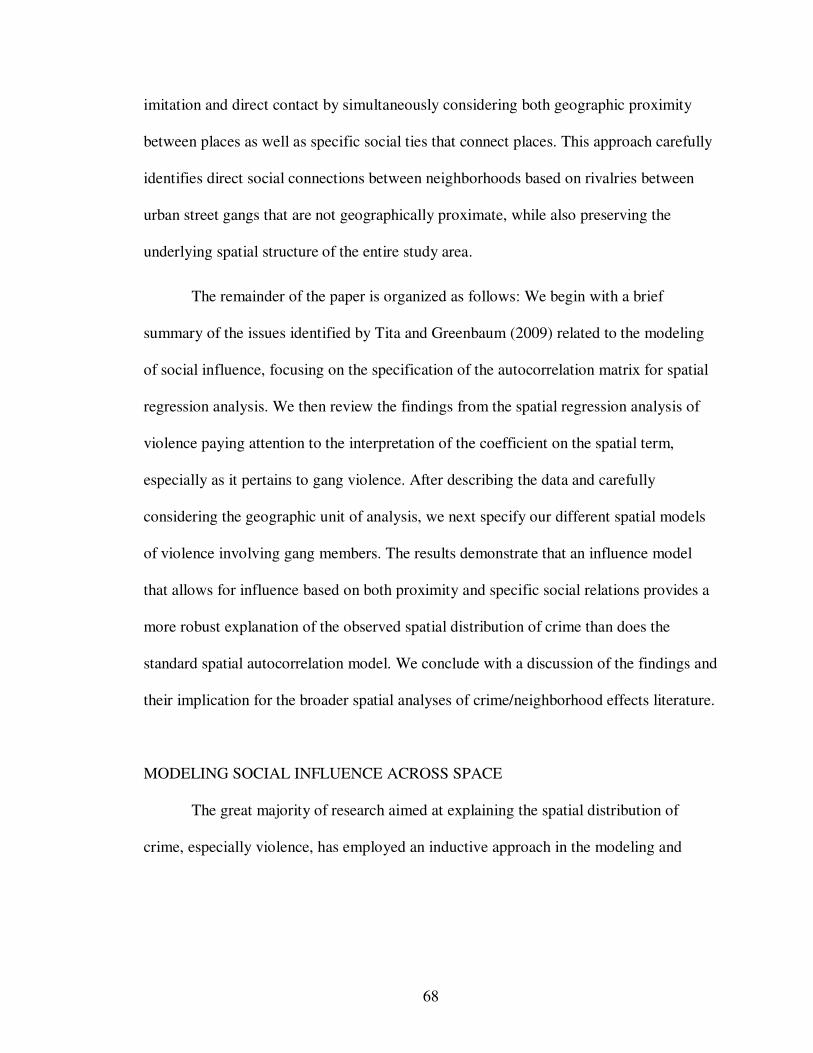
68

imitation and direct contact by simultaneously considering both geographic proximity

between places as well as specific social ties that connect places. This approach carefully

identifies direct social connections between neighborhoods based on rivalries between

urban street gangs that are not geographically proximate, while also preserving the

underlying spatial structure of the entire study area.

The remainder of the paper is organized as follows: We begin with a brief

summary of the issues identified by Tita and Greenbaum (2009) related to the modeling

of social influence, focusing on the specification of the autocorrelation matrix for spatial

regression analysis. We then review the findings from the spatial regression analysis of

violence paying attention to the interpretation of the coefficient on the spatial term,

especially as it pertains to gang violence. After describing the data and carefully

considering the geographic unit of analysis, we next specify our different spatial models

of violence involving gang members. The results demonstrate that an influence model

that allows for influence based on both proximity and specific social relations provides a

more robust explanation of the observed spatial distribution of crime than does the

standard spatial autocorrelation model. We conclude with a discussion of the findings and

their implication for the broader spatial analyses of crime/neighborhood effects literature.

MODELING SOCIAL INFLUENCE ACROSS SPACE

The great majority of research aimed at explaining the spatial distribution of

crime, especially violence, has employed an inductive approach in the modeling and

69

explanation of findings.14 That is, the structure of influence between communities is

modeled geographically using rook’s or queen’s case contiguity. The implication is that

space matters, but that influence is constrained by distance and that nearest neighbors

matter most (also known as “Tobler’s First Law of Geography” (Tobler 1970)). If the

coefficient on the spatial terms is statistically significant, post-hoc explanations centered

on contagion (Loftin 1986), exposure (Morenoff et al. 2001; Griffiths and Chavez 2004),

gangs (Rosenfeld et al. 1999; Cohen and Tita 1999), and drug markets (Morenoff and

Sampson 1997; Cork 1999; Tita and Cohen 2004) have been advanced as the possible

mechanisms responsible for the spatial clustering of events. Though these studies have

been invaluable in empirically demonstrating the existence of unobserved contextual or

“neighborhood effects”, very little progress has been made in moving these unobserved

neighborhood effects into the realm of the observable. To take this next step, Tita and

Greenbaum (2009) argue for the adoption of deductive approach in model construction.

The key element in identifying the way that “influence” matters in spatial

regression models is the autocorrelation–or spatial weights–matrix, represented by W,

which captures the structure linking persons, places, or things together. Part of the reason

that the mechanisms of influence remain unidentified is related to the way in which the

autocorrelation matrix is specified in spatial analysis. Restricting processes of influence

to operate only among contiguous neighbors is to ignore processes of influence that are

inherently more complex in terms of the spatial extent of interactions (e.g. Sampson

2004). A more deductive approach would consider both the social and the geographic

structure of the data and incorporate these complexities into the spatial weights matrix.

14 For a detailed review and critique of inductive approaches to modeling influence across space see Tita and Greenbaum (2009).

70

The construction of W is extremely important in terms of identifying the mechanisms

driving influence processes. As Leenders (2002:22) notes: “W is supposed to represent

the theory a researcher has about the structure of the influence processes in the network.

Since any conclusion drawn on the basis of autocorrelation models is conditional upon

the specification of W, the scarcity of attention and justification researchers pay to the

chosen operationalization of W is striking and alarming. This is especially so, since

different specifications of W typically lead to different empirical results.” Put more

succinctly, “Change one’s theory, change W” (Leenders 2002:26.)

A deductive approach built on the understanding that social networks are

inherently geographic, existing both within and across localities and connecting

communities separated by distance (e.g. Ettlinger and Bosco 2004), offers a promising

framework for advancing our understanding of why space matters. This analytic

framework allows influence to take place not just between geographically proximate

neighbors (as with conventional spatial analysis) but also between locations that are

connected by social networks. By carefully considering and allowing for processes that

extend beyond (or perhaps preclude) spatially adjacent areas, one can ensure that the

spatial weights matrix adequately captures the realities of the mechanisms of influence.

Just as Morenoff (2003:997) argues that spatial analysis “…expands the neighborhood-

effects paradigm by considering not only the local neighborhood but also the wider

spatial [emphasis added] context within which that neighborhood is embedded”, we

argue that careful consideration of the socio-spatial dimensions of social influence will

facilitate the inclusion of the “wider social context of neighborhoods” into the

neighborhood effects literature.

71

Outside of the examination of crime, there are several examples of innovative

efforts that recognize that the processes of influence are not neatly bounded by, or limited

to, spatially adjacent areas. Gould (1991) finds that overall levels of resistance during the

Paris Commune of 1871 were not influenced by levels of resistance in neighboring areas.

Instead, resistance levels were greatest among those districts (arrondissements) that

shared enlistments. The sharing of resources (resistance fighters) increased solidarity,

which translated into greater overall effectiveness in the local insurgency’s effort. More

recently, Greenbaum (2002) explored the spatial distribution of wages among teachers in

Pennsylvania. He finds that teachers’ wages are more alike when contiguity among

school districts is based upon socio-economic similarities rather than geographic

contiguity. That is, wages in non-adjacent affluent school districts exhibit similar wages

when compared to adjacent but non-affluent school districts. State level budgets and

fiscal policy are also known to be related to the expenditures and policies of

“neighboring” states (Case et al. 1993.) Not only are expenditures similar among spatially

adjacent states, but they are also similar among states that are identified as “neighbors”

because they share similarity in terms of median income and racial composition.

There are fewer examples of studies that “unbound” space within the

criminological literature. In addition to the work of Tita and Greenbaum (2009), Mears

and Bhati (2006) link adjacent as well as non-adjacent areas to one another if the

residents are economically and demographically similar. The stated goal of their research

is not to examine “…spatial diffusion processes, wherein violence in one community

causes crime in another. Rather, [they] examine whether resource deprivation exerts an

influence on violent crime in other communities” (Mears and Bhati 2006:2). On the basis

72

of “homophily” (Blau and Blau 1982; McPherson et al. 2001), they posit that behaviors

in a focal area will be influenced by behaviors in socially similar areas because social

similarity increases the probability of interactions among individuals. Mears and Bhati

(2006) test this by constructing an autocorrelation matrix based on “similarity” that links

socially similar areas together regardless of spatial proximity. This work is an important

advance in the modeling of influence by a general contagion process which too often

assumes that transmission by social networks occurs through the direct social contact

among individuals residing only in spatially adjacent communities (Lofton 1986;

Morenoff 2003). Recent work by Papachristos (2007) focuses more on how the structure

of gang networks in Chicago influences the pattern of intra- and inter-gang violence.

Controlling for spatial adjacency and contested territory, this work demonstrates that

proximity between gangs is a strong predictor of retaliatory behavior.

Although as Feld (1981) notes, geographic proximity among individuals can

create opportunities for the interactions that constitute social networks, it is not clear that

modeling social influence through geographic distance or proximity alone adequately

captures the full range of social interactions that researchers believe to be important (see

also Reiss and Farrington 1991). The importance of considering ties across

geographically distant but socially similar places is further underscored by Sampson and

Sharkey (2008) who demonstrate that intra-metropolitan residential mobility patterns are

largely confined by either class, race or, in the case of African-Americans, both.

73

MODELING SPATIAL PATTERNS OF VIOLENCE

Two consistent findings have emerged from the spatial analysis of violence

literature. First, the subpopulation at greatest risk of homicide victimization is comprised

of young urban minority males. Second, homicides exhibit a non-random pattern of

positive spatial concentration, meaning that areas with similar levels of violence cluster

in space. This pattern has been interpreted as evidence of diffusion, or the spread of

violence over space and through time. As noted above, inductive approaches have

proffered a variety of mechanisms responsible for the diffusion of crime including

exposure and the social organization of drug markets. Though these are highlighted

elsewhere (see Tita and Greenbaum 2009), the current research focuses specifically on

the role of urban street gangs in explaining the spatial distribution of violence (see

Decker 1996; Wilkinson and Fagan 1996; Cohen et al. 1998; Cohen and Tita 1999;

Rosenfeld et al. 1999; Morenoff et al. 2001; Griffiths and Chavez 2004; Tita and Cohen

2004; Papachristos 2007).

One reason that the presence of an urban street gang has emerged as one of the

most common mechanisms implicated as a source of spatial dependence and the spatial

distribution of violent crime is that gang-related homicide demonstrates patterns of

positive spatial autocorrelation on a more consistent basis than do other types of

homicides (Cohen et al 1998; Cohen and Tita 1999; Rosenfeld et al. 1999). This nexus

between gangs and the geography of violent crime rests upon two defining features of

gangs. First, gangs are geographically oriented in that they have a strong attachment to

the territory, or turf, under their direct control. Further, while the total territorial area

claimed by a gang may be quite large and vary over time, the “set space” where urban

74

street gangs come together is a well-defined, sub-neighborhood area that remains

consistent over time (Klein 1995; Moore 1985, 1991; Tita et al. 2005). Second, behaviors

associated with the control of territory, such as communicating turf boundaries,

regulating activities within turf, and defending turf against rivals, are important elements

in the diffusion of violence (Sack 1986; Newman 2006; Papachristos 2007). In the

process of controlling territorial space, gangs have negative relations (i.e., rivalries) that

explicitly tie them to other gangs and to other territories, turfs, and set spaces. The

combination of a gang’s persistent geographic presence and the territorial behaviors

required to defend, maintain, or expand turf help diffuse certain types of violence in

urban settings.

While the territorial claims and behaviors of gangs can be understood as an

important geographic component to the theory of the spatial distribution of violence,

gang turf itself is not an ideal choice as a spatial unit of analysis. Issues surrounding the

selection of units of analysis when using data grouped or aggregated to geographical

areas, such as border effects or the modifiable areal unit problem, are ever present and,

like any area partitioned into discrete units by politically-minded boundaries, gang turf is

less than optimal for spatial analysis.15 Recognizing the importance of the geographic

unit of analysis to analytic outcomes when using spatially aggregated socio-economic

data, we took steps in data collection to mitigate common issues of unit selection in

spatial analysis. Through the use of address-matching in a geographic information system

15 Border effects refer to the fact that the often-arbitrary boundaries of study regions may exclude information that affects outcomes within the study region (see Griffith 1983). The modifiable areal unit problem refers to the fact that the results of statistical analysis, such as correlation and regression, can be sensitive to the geographic zoning system used to group data by area (see Gehlke and Behl (1934) or Robinson (1950) for classic examples of MAUP, or Openshaw (1996) for a more contemporary review). While well-established in geography, these issues tend to resurface in other disciplines as spatial analysis becomes more prevalent (for example, see Hipp 2007). For a review of the treatment of these issues in the spatial analysis of crime, see Weisburd et al. (2009).

75

(GIS), each incident in our crime data is precisely located in space rather than already

aggregated to an areal unit. This has the positive effect of freeing subsequent analysis

from the use of any particular unit of analysis, allowing the researcher to select a unit that

best fits the aims of the research question. We made use of this flexibility in a very

specific fashion in this project by overlaying a census block group geography over the

gang turf geography. By doing so we were able to rescale the unit of analysis from

relatively large areas of gang turf into smaller scale census units. Gang turf claims and

violence counts were then assigned to the census units along with aggregate-level socio-

economic data. By making use of precisely located crime data, we were able to rescale

the unit of analysis, enabling us to examine both compositional and contextual elements

of the diffusion of gang violence while helping to mitigate common issues of unit

selection in spatial analysis.

Together, the territorial geography of gangs and their social network of rivalries

suggest a set of structural properties that researchers have not adequately exploited in

terms of understanding the spatial structure of gang violence. As Tita and Greenbaum

(2009) point out, this oversight is unfortunate given the existence of social network

analyses of gangs which have been used to guide the development and implementation of

problem-solving/gun violence reduction strategies (see Kennedy et al. 1997; Tita et al.

2002; McGloin 2005). By combining the gang turf geography with information on the

social networks between those gangs, it becomes possible to determine whether rival

gangs are located in spatially adjacent areas. If the socio-spatial dynamics of gang enmity

are more complex – meaning that they span simple geographic proximity and serve as

76

mechanisms that can link non-contiguous areas—then the spatial dependence matrix

should be specified such that it is able to capture these complexities.

The goal of this research is to better understand the spatial distribution of one type

of violence: that which is perpetrated by and/or against gang members. Drawing from

existing theories and empirical evidence from the gang literature and the spatial analysis

of violence literature, two models are specified. The first model follows the conventional

approach and limits the influence of violence in other area on a focal area by restricting

the impact among only spatially adjacent areas. The second model considers the socio-

spatial dimensions of gangs, which combines spatial data on gang locations with social

network data on gang rivalries. In specifying our social process (gang rivalry, retaliation)

a priori, we construct a spatial autocorrelation matrix that links observations (census

block groups) only when each pair of places contains the gang set space of rival gangs.

The central question, then, is this: Does modeling spatial dependence using spatial

adjacency best account for the distribution of gang violence, or are additional insights

gained by explicitly considering the socio-spatial dimension of gangs and their rivalries?

If violence committed by gang members in a neighborhood is influenced by the actions of

rival gang members, and if gang rivalries extend beyond geographic neighbors, one might

expect the network-based matrix to better explain the observed spatial distribution of

crimes in the study area.

Tita and Greenbaum (2009) are careful to note that spatial adjacency may still

play an important role in explaining spatial patterns of gang-involved violence. Given

that gang members commit more violent crimes than do non-gang members (see

Thornberry et al. 2003), a community that is exposed to gang members is likely to exhibit

77

higher levels of violence. Therefore, any geographic clustering of gang territories should

produce spatial autocorrelation in gang violence across the geography. We contend,

however, that diffusion driven by the social interactions among gangs involved in

ongoing rivalries may also (or perhaps, better) explain the observed spatial patterning of

violence involving gang members, especially if the violence is primarily gang motivated

and retaliatory in nature. The extent to which the interaction patterns of gang rivalries

span simple contiguity to encompass non-contiguous areas should inform the

specification of one’s spatial weights matrix.

RESEARCH DESIGN AND MEASUREMENT

The empirical analysis is conducted using census block group data and geo-coded

crime data provided by the Los Angeles Police Department (LAPD) for the Hollenbeck

Policing Area (see Figure 4.1.) Hollenbeck encompasses roughly fifteen (15) square

miles and has a population of approximately 170,000. Most of the population is Latino

(84.5%) and the vast majority are of Mexican descent (82.6%) – half (39.4%) of whom

were born in Mexico. The median household income in Hollenbeck is $27,096 and thirty

percent of the population lives below the poverty line. Of the total population that is

twenty-five years old or older, thirty five percent have less than a high school degree (or

equivalent).

Because of physical and geo-political barriers, Hollenbeck is ecologically distinct

from neighboring areas. For instance, on the western border the Los Angeles River

separates Hollenbeck from downtown Los Angeles. To the south, Hollenbeck borders the

city of Vernon, which has a total population of less than 100 and is dominated by

78

meatpacking and other industrial sites. The unincorporated area of Los Angeles

commonly referred to as “East Los Angeles” as well as the city of Pasadena border

Hollenbeck to the east/northeast. In addition to the Los Angeles River, numerous

freeways dissect Hollenbeck differentiating it from other parts of Los Angeles and

creating ecologically distinct neighborhoods within Hollenbeck (e.g., “Boyle Heights”,

“Lincoln Heights” and “El Sereno”). As demonstrated elsewhere (see Tita et al. 2002;

Tita et al. 2003), these borders serve to create a landscape within which the rivalries of

the Hollenbeck gangs are wholly contained. As a result, the current research does not

suffer from the sort of “boundary effect” inherent in most examples of spatial analysis

that are not dealing with a complete social and geographical system.16

Hollenbeck has a long and well-studied history of urban street gangs with some of

the gangs originating before the Second World War. Joan Moore (1985, 1991) has

written extensively on one of the oldest gangs in the neighborhood, White Fence, while

other gangs have been the focus of such notable gang researchers as Malcolm Klein

(1971) and James Diego Vigil (1988, 2002). The gangs in Hollenbeck are “traditional

gangs” (Klein 1995) and have a strong attachment to turf. Violence in Hollenbeck is

expressive in nature, with much of it tied to the defense of one’s turf (see Tita et al.

2002.) During the research period, between 2000 and 2002, twenty-nine “criminally

active” street gangs were identified in Hollenbeck. All other groups such as “tagger

crews”, “skate punks” and “stoners” were excluded on the basis that, according to local

police, they do not participate in violence and they are not territorially defined.

16 City-level studies of violence, for instance, often exclude data from spatially contiguous areas located just beyond the focal city’s borders not because these areas are unimportant, but rather because the data may not be available. Because none of the rivalries extend to gangs that lie beyond the borders of the research site, there are no non-Hollenbeck rival gangs to be excluded thereby ensuring that the full extent of the social process believed to matter (gang rivalries) is being captured.

79

Measures of Gang Turf

Identifying and mapping the territorial claims of the gangs was made possible by

working with detectives and patrol officers assigned to LAPD’s Hollenbeck gang unit as

well as Los Angeles County probation officers whose caseload was comprised

exclusively of Hollenbeck gang members. These gang experts were given detailed, large-

scale maps for each of the fifty-six “reporting districts” and then asked to draw the

boundaries of each gang. This information was transferred to a geographic information

system (GIS) which enabled us to layer a map of census block group boundaries over the

gang turf map. We were thus able to disaggregate the turf map and locate the presence or

absence of a gang at the census block group level – a level at which evidence suggests is

meaningful in the ecological study of gangs (see Tita et al. 2005; Tita and Ridgeway

2007). Of the 120 census block groups included in this study, gangs claimed at least some

portion of 103 block groups. In seven instances, two gangs claimed parts of the same

block group; sometimes these gangs were rivals, sometimes they were simply

“neighbors.”

Measurement of Gang Rivalries

A list-sort technique was used to identify the rivalries that link the gangs. Each

informant was provided with a survey comprised of one page for each gang. At the top of

the page, a particular gang was identified and the respondent was asked to “Please

Identify All of the Gangs that are an Enemy of the <insert gang name>.” In addition to

the law enforcement experts, several current and former members of gangs also

80

completed the survey network form. Gang members were accessed through an

employment/training center and its founder, a nationally known Jesuit Priest who works

with gang members from Hollenbeck and surrounding areas. Though only members from

six of the 29 gangs completed surveys, there was perfect agreement across the gang

members’ and law enforcement experts’ surveys regarding the enmity connections

between gangs. A sociogram depicting the structure of the gang rivalries is provided in

Figure 4.2

Measures of Gang Violence

The dependent variable includes all violent crimes committed by or against gang

members in the Hollenbeck Policing Area between May of 2000 through December of

2002.17 Therefore, the violence is “gang related” and includes both “gang motivated”

violence (e.g., protection of turf from an incursion by rival members) as well as all other

violence involving a gang member. The total number of crimes included in the study is

1,223, or an average of 10.2 violent gang crimes per block group (n=120) over the thirty-

month period. The crime types included in the file are all aggravated assaults, simple

assaults, assault with a deadly weapon, attempted homicides, homicides, robberies,

kidnappings, and firing a gun into an inhabited dwelling/vehicle. The spatial distribution

of these crimes is presented in Figure 4.3. Rape and instances of domestic violence are

excluded from this analysis because the data were unavailable. Sexual and/or domestic

17 Research has demonstrated that in this area of Los Angeles, gang involved violence accounts for 75% of all lethal violence (see Tita et al. 2003). Additionally, the current analysis was performed on all violent crimes regardless of gang involvement. Not surprisingly in light of the gang dominance in the commission of violent acts, there were no differences. These analyses are available from the authors upon request.

81

violence is also less likely to be influenced by either exposure or diffusion processes

operating at the neighborhood level.

Ecological Measures

Included in the models is a set of commonly used indicators of neighborhood

structural composition associated with high levels of homicide (Land et al. 1990; Krivo

and Peterson 1996). Specifically, the following 2000 census variables are included in the

analysis: the percentage of residents that are of Hispanic origin, the median household

income, the percentage of households that are headed by females, the percentage of

residents who rent, the percentage of adults over the age of twenty-five with less than a

high school (or GED) degree, the percentage of residents who moved into the community

in the last five years, the percent of housing units that are vacant, the percentage of

residents between the crime prone ages of fourteen to twenty-four years of age, and

population density. A dichotomous variable to distinguish among high poverty (between

twenty and forty percent of the population in poverty) and extreme poverty (at least forty

percent of the population living in poverty) neighborhoods from low poverty

neighborhoods was also constructed (see Krivo and Peterson 1996). Finally, the model

controls for the area (square miles) of the census block group. Descriptive statistics for

the independent variables, along with the dependent variable, are presented in Table 4.1.

Measurement of the Weights Matrix

82

The geographically based spatial weights matrix (Wg) is based on rook’s case

first-order contiguity and was constructed using the GeoDa software (version 0.95i) for

spatial analysis (Anselin et al. 2006).18 We settled on this specification after specifying

several different spatial configurations and then examining the amount of spatial

autocorrelation in the number of gang crimes per block group. The most common statistic

used to determine the overall pattern of spatial autocorrelation is Moran’s I, which is very

similar to a simple correlation coefficient. The formula is given by:

2)(/))(( µµµ −∑−−∑∑= iijiijji xxxwI

The test statistic, I, is bounded by 1.0 (perfect positive autocorrelation meaning

the spatial clustering of like values) and –1.0 (perfect negative autocorrelation meaning

dissimilar values cluster spatially.) Both rook’s case (neighbors defined by shared border

lengths) and queen’s case (neighbors defined by a shared border point) configurations

were tested for first-order neighbors (those that are immediately contiguous to the focal

unit), second-order neighbors (those that are immediately contiguous to the focal unit’s

first-order neighbors), and first- and second-order neighbors combined. The Moran’s I

results for these different configurations are presented in Table 4.2.

Based on these results, it is clear that the spatial autocorrelation of gang crime

diminishes quickly across space when using census block group geography. Crime counts

show weak but statistically significant measures of positive spatial autocorrelation for

rook’s case first-order neighbors (I = 0.0907 with a significance level of 0.047), but when

18 As discussed previously, we theorize that the territoriality of gangs is at the heart of rivalry relations between gangs. However, we do not limit the Wg matrix to include only units already claimed by neighboring gangs. We see areas that were unclaimed at the time of the study as something that gangs may compete over as well.

83

second-order neighbors are considered, the results show weakly negative spatial

autocorrelation. Based on these results, rook’s case first-order contiguous neighbors form

the Wg. The weights matrix can also be depicted as a network drawing where the nodes

are the block groups and an edge between block groups means that they are adjacent (see

Figure 4.4).

The second weights matrix employed in this research is derived from the ties

within the enmity network and the spatial location of the gangs’ activity space (i.e., turf

or “set space”). This matrix, Wn, was constructed by first creating a location-by-gang

matrix with dimensions of m x n (120 block groups x 29 gangs). The dark colored nodes

in the network diagram in Figure 4.5 represent the gangs while the lighter shaded nodes

presents each of the census block groups. This matrix was then multiplied by the n x n

(29 x 29) enmity network followed by the transpose of the location-by-gang matrix (29 x

120). After executing the matrix algebra one is left with a two-mode, m x m (120 x 120)

matrix that identifies census block groups that are “enemies” of one another. That is, a

non-zero value in a cell of Wn indicates that the pair of block groups is linked because

they both contain the turf of rival gangs.

Repeating the Moran’s I analysis but using the network derived weights matrix,

Wn, I = 0.124 and is statistically significant at the 0.015 level. While Moran’s I tests for

both Wg and Wn demonstrate positive spatial autocorrelation, the test statistic is larger

when the network-based W is used. However, it is incorrect to evaluate the two

approaches based upon the magnitude of Moran’s I without also examining the

significance levels. Because the significance level is greater for Wn, the level of spatial

84

autocorrelation is more consistent with the socio-spatial dimensions of gang rivalries

rather than the simple contiguity-based measure of influence.

Figure 4.6 provides a visualization of the network-derived weights matrix (Wn).

Yet this picture is deceptive because many of the nodes (census block groups) are, in

network terms, structurally equivalent.19 That is, every block group that contains the turf

of gang “A” is tied in exactly the same way with every other block group that contains

the turf of “A’s” rival. This is demonstrated graphically in Figure 4.7 where the same

node, #11, identified in the circle in Figure 4.6, has been “spread out” to show that there

were actually two other nodes (#5 and #7) that are also tied to exactly the same set of

nodes. Thus, the network matrix is no longer a fully connected binary matrix where every

unit has at least one neighbor, but instead one where some block groups have no

neighbors while others have multiple ties to the same block group (as in the case where

multiple gangs share the same block group and also share a common enemy.)

MODELS OF GANG VIOLENCE

To model the impact of both geographical space and social space on the spatial

distribution of gang involved violence, we use a spatial dependence model, also

commonly referred to as a “spatial lag” model. While the spatial error model is

appropriate when one is concerned about unmeasured endogenous effects among

spatially proximate areas, given that we are interested in exploring two specific

19 The two most common approaches to equivalence in network analysis are structural equivalence and regular equivalence. The most important difference between the two is that structural equivalence requires that equivalent actors have the same connection to the same neighbors while regular equivalent actors have the same or similar patterns to potentially different neighbors (see Doreian et al. 2005).

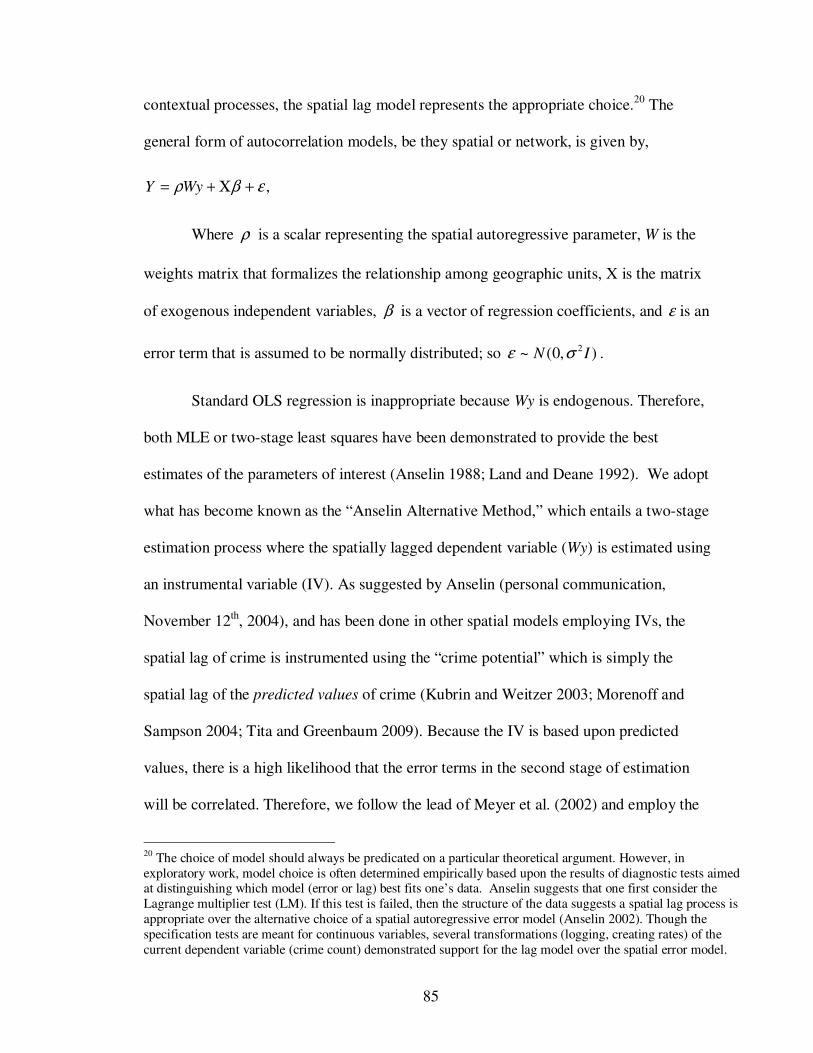
85

contextual processes, the spatial lag model represents the appropriate choice.20 The

general form of autocorrelation models, be they spatial or network, is given by,

,εβρ +Χ+= WyY

Where ρ is a scalar representing the spatial autoregressive parameter, W is the

weights matrix that formalizes the relationship among geographic units, X is the matrix

of exogenous independent variables, β is a vector of regression coefficients, and ε is an

error term that is assumed to be normally distributed; so ),0(~ 2 IN σε .

Standard OLS regression is inappropriate because Wy is endogenous. Therefore,

both MLE or two-stage least squares have been demonstrated to provide the best

estimates of the parameters of interest (Anselin 1988; Land and Deane 1992). We adopt

what has become known as the “Anselin Alternative Method,” which entails a two-stage

estimation process where the spatially lagged dependent variable (Wy) is estimated using

an instrumental variable (IV). As suggested by Anselin (personal communication,

November 12th, 2004), and has been done in other spatial models employing IVs, the

spatial lag of crime is instrumented using the “crime potential” which is simply the

spatial lag of the predicted values of crime (Kubrin and Weitzer 2003; Morenoff and

Sampson 2004; Tita and Greenbaum 2009). Because the IV is based upon predicted

values, there is a high likelihood that the error terms in the second stage of estimation

will be correlated. Therefore, we follow the lead of Meyer et al. (2002) and employ the

20 The choice of model should always be predicated on a particular theoretical argument. However, in exploratory work, model choice is often determined empirically based upon the results of diagnostic tests aimed at distinguishing which model (error or lag) best fits one’s data. Anselin suggests that one first consider the Lagrange multiplier test (LM). If this test is failed, then the structure of the data suggests a spatial lag process is appropriate over the alternative choice of a spatial autoregressive error model (Anselin 2002). Though the specification tests are meant for continuous variables, several transformations (logging, creating rates) of the current dependent variable (crime count) demonstrated support for the lag model over the spatial error model.

86

Murphy and Topel (1985) correction to the standard errors in the second stage of

estimation. The estimation of this model was completed using Stata 8.2 SE (StataCorp

2005) and the “QVF” routine that fits generalized linear models using IRLS (maximum

quasi-likelihood). The model is estimated by specifying the negative binomial as the

underlying distribution of the dependent variable and the link function is set equal to the

log function.

We estimate four models. First, in order to obtain the predicted values for the

number of crimes in each block group, gang violence is modeled only as a function of the

community-level (block group) structural variables as follows:

1.) (Eq AreaCrimeAge%

NoHSPopDensityHighPovExtremePovVacantProp%

NewRes%Renters%FemHH%MedHHIncHispanic%

1211

109876

543210

εββ

βββββ

ββββββ

++

+++++

++++++=Y

To test whether gang involved violence in a focal neighborhood is influenced by

levels of such violence among contiguous units, we next use the predicted values of

crime ( y ) multiplied by the spatial weights matrix, Wg, as an IV (for the regular spatial

lag of crime counts, Wgy) in the second-stage of estimation.

2.) (Eq AreaCrimeAge%

NoHSPopDensityHighPovExtremePovVacantProp%

NewRes%Renters%FemHH%MedHHIncHispanic%ˆ

1211

109876

543210

εββ

βββββ

βββββρβ

++

+++++

+++++++= yWY G

The third model examines the socio-spatial dynamics of gang rivalries on

observed patterns of violence involving gang members. This model is identical to

Equation 2 except the IV is a function of the weights matrix based upon the network ties

linking geography (Wn) and the predicted values of y.

87

3.) (Eq AreaCrimeAge%

NoHSPopDensityHighPov ExtremePovVacantProp%

NewRes%Renters%FemHH%MedHHIncHispanic%ˆ

1211

109876

543210

εββ

βββββ

βββββρβ

++

+++++

+++++++= yWY n

The final model includes both the spatially lagged and socially lagged predicted

values as the IV for their respective spatial lags and is defined as:

4.) (Eq AreaCrimeAge%

NoHSPopDensityHighPovExtremePovVacantProp%

NewRes%Renters%FemHH%MedHHIncHispanic%ˆˆ

1211

109876

543210

εββ

βββββ

βββββρρβ

++

+++++

++++++++= yWyWY ng

RESULTS

The results of the regressions are presented in Table 4.3. In the non-spatial model

used to obtain the predicted values to be used as IV’s, poverty and female-headed

household are found to be statistically significant predictors of gang crime. Similarly,

block groups with a higher proportion of Hispanics and those with greater population

density also experience higher levels of gang violence. We included the percentage of

Hispanic residents to control for the geography of project housing in the study area.

While the overall demographic composition of the study area is largely Hispanic, there is

considerable variation in the percentage of Hispanic residents at the scale of block groups

and the units with the highest percentages of Hispanic residents largely track with the

presence of housing projects. These results are consistent with other findings in the

literature that show areas with higher levels of resource deprivation suffer higher levels

of violent crime (Krivo and Petersen 1996; Morenoff et al. 2001; Mears and Bhati 2006).

Similarly, population density, an indicator of informal local social control, is positively

associated with crime and violence. Counter to expectations, areas with a higher

88

percentage of the population renting experience lower levels of gang crime. We also find

that larger census block groups contain more gang crime.

When the spatially lagged crime variable is added to the model, poverty measures

(+), the percent Hispanic (+), and the percent renting (-) continue to be statistically

significant. The spatial lag, however, sits right at the cusp of statistical significance

(t=0.068). Although this variable is often found to be statistically significant in the

analysis of aggregate levels of lethal and non-lethal violence (Morenoff and Sampson

1997; Rosenfeld et al.1990; Baller et al. 2001; Morenoff and Sampson 2004), this does

not appear to be the case when the focus is specifically on gang violence. This finding is

consistent with the results achieved by Mears and Bhati (2006), but contradicts the de

facto explanations offered in most studies of the spatial distribution of all types of

homicide that often evoke “gangs” as one of the chief contributors to the positive spatial

dependence among events.

By replacing the lagged crime variable created using the contiguity matrix (Wg)

with the lagged crime variable produced using the network based measure (Wn), we find

that poverty is significant. Consistent with the results from the first two models, a larger

concentration of Hispanic residents is also significantly associated with higher levels of

gang violence. Once again we find that larger areas are more likely to contain a greater

number of incidents. Most importantly, the network based spatial lag variable is positive

and significant. This suggests that gang rivalries do indeed impact the observed spatial

distribution of gang violence, but that such linkages matter in ways that extends well

beyond simple spatial contiguity.

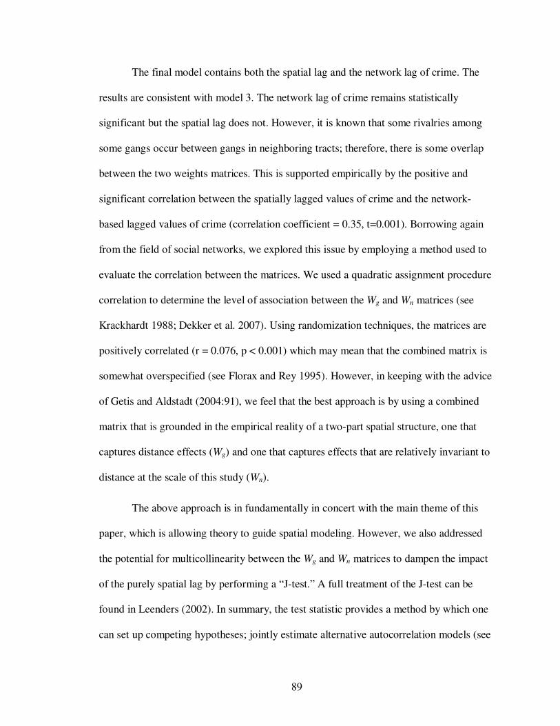
89

The final model contains both the spatial lag and the network lag of crime. The

results are consistent with model 3. The network lag of crime remains statistically

significant but the spatial lag does not. However, it is known that some rivalries among

some gangs occur between gangs in neighboring tracts; therefore, there is some overlap

between the two weights matrices. This is supported empirically by the positive and

significant correlation between the spatially lagged values of crime and the network-

based lagged values of crime (correlation coefficient = 0.35, t=0.001). Borrowing again

from the field of social networks, we explored this issue by employing a method used to

evaluate the correlation between the matrices. We used a quadratic assignment procedure

correlation to determine the level of association between the Wg and Wn matrices (see

Krackhardt 1988; Dekker et al. 2007). Using randomization techniques, the matrices are

positively correlated (r = 0.076, p < 0.001) which may mean that the combined matrix is

somewhat overspecified (see Florax and Rey 1995). However, in keeping with the advice

of Getis and Aldstadt (2004:91), we feel that the best approach is by using a combined

matrix that is grounded in the empirical reality of a two-part spatial structure, one that

captures distance effects (Wg) and one that captures effects that are relatively invariant to

distance at the scale of this study (Wn).

The above approach is in fundamentally in concert with the main theme of this

paper, which is allowing theory to guide spatial modeling. However, we also addressed

the potential for multicollinearity between the Wg and Wn matrices to dampen the impact

of the purely spatial lag by performing a “J-test.” A full treatment of the J-test can be

found in Leenders (2002). In summary, the test statistic provides a method by which one

can set up competing hypotheses; jointly estimate alternative autocorrelation models (see

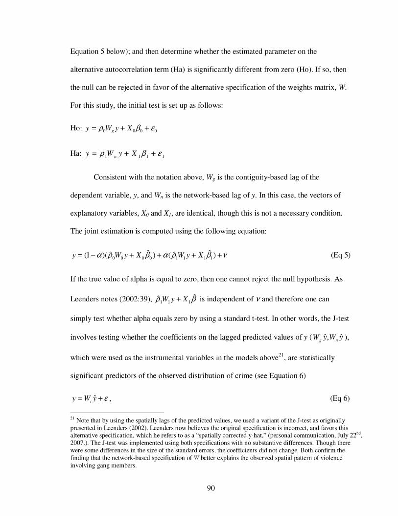
90

Equation 5 below); and then determine whether the estimated parameter on the

alternative autocorrelation term (Ha) is significantly different from zero (Ho). If so, then

the null can be rejected in favor of the alternative specification of the weights matrix, W.

For this study, the initial test is set up as follows:

Ho: 0000 εβρ ++= XyWy g

Ha: 1111 εβρ ++= XyWyn

Consistent with the notation above, Wg is the contiguity-based lag of the

dependent variable, y, and Wn is the network-based lag of y. In this case, the vectors of

explanatory variables, X0 and X1, are identical, though this is not a necessary condition.

The joint estimation is computed using the following equation:

νβραβρα ++++−= )ˆˆ()ˆˆ)(1( 11110000 XyWXyWy (Eq 5)

If the true value of alpha is equal to zero, then one cannot reject the null hypothesis. As

Leenders notes (2002:39), βρ ˆˆ 111 XyW + is independent of ν and therefore one can

simply test whether alpha equals zero by using a standard t-test. In other words, the J-test

involves testing whether the coefficients on the lagged predicted values of y ( yWyW ngˆ,ˆ ),

which were used as the instrumental variables in the models above21, are statistically

significant predictors of the observed distribution of crime (see Equation 6)

=y ε+yWiˆ , (Eq 6)

21 Note that by using the spatially lags of the predicted values, we used a variant of the J-test as originally presented in Leenders (2002). Leenders now believes the original specification is incorrect, and favors this alternative specification, which he refers to as a “spatially corrected y-hat,” (personal communication, July 22nd, 2007.). The J-test was implemented using both specifications with no substantive differences. Though there were some differences in the size of the standard errors, the coefficients did not change. Both confirm the finding that the network-based specification of W better explains the observed spatial pattern of violence involving gang members.

91

where Wi is either the network-based measure of dependence or the contiguity-based

measure of dependence. The researcher is free to specify either autocorrelation matrix

under the null hypothesis. To insure that the conclusion one reaches is not simply a

byproduct of which matrix is chosen as the null, the specifications of the null and

alternative are reversed and Equation 6 is estimated a second time.

The null hypothesis is initially specified under the condition in which the

predicted spatially lagged variables were constructed using the spatial contiguity matrix

(Wg). As reported in Table 4.4, the coefficient on the lagged spatial term is not

statistically significant (t=0.151.) Therefore, one cannot reject the null hypothesis that the

true value of alpha = 0. It does not follow, however, that the geographically based

weights matrix (Wg) provides a better measure of dependence than does the network-

based measure (Wn). To test which specification of the weights matrix better predicts the

outcome, the null hypothesis is then specified using the lagged network term. Under this

specification the coefficient on the lagged predicted values is found to be statistically

significant at the t=0.001 level. It is now possible to reject the null hypothesis that alpha

is equal to zero in favor of the alternative. Therefore, we rejected the hypothesis that Wg

is correct in favor of the alternative that Wn is the more appropriate specification of the

autocorrelation/dependence matrix.

CONCLUSIONS

A growing number of studies in the social sciences have adopted spatial

regression in an effort to model and understand neighborhood effects (see Sampson et al.

92

2002; Ward and Gleditsch 2008).22 In criminology, these efforts have used spatially

lagged variables as proxies for various social phenomena thought to be responsible for

the consistent finding that spatial clustering of crime events remains even after

controlling for place-to-place variations in compositional effects such as race, ethnicity

and poverty. While we see these efforts as a positive first step toward a “spatially

integrated” criminology (see Goodchild et al. 2004), the way in which space is

incorporated requires careful consideration. Specifications of the spatial weights matrix

that rely on spatial contiguity to define the spatial reach of the various social processes

posited to be responsible for clustering forces researchers to assume that all such

processes decay rapidly over geographic distance, and therefore matter only among

spatially contiguous neighbors. Furthermore, even when multiple social processes are

considered, the conventional modeling approach is to specify a single spatial weights

matrix rather than specify different kinds of connections between places for different

social processes. In addition to making it impossible to parse the impact of one process

from that of another, this is an atheoretical approach to understanding why and how space

matters (Leenders 2002).

Building on these perspectives, this research focuses on the particular outcome of

violence involving gang members and demonstrates that “space” continues to matter as

the compositional characteristics of places cannot adequately account for the overall

geographic patterns of violence. And while our findings also verify that researchers have

22 We are sensitive to arguments that quantitative modeling is not the only way to approach issues of crime in place specific settings. Although the methods demonstrated in this article are capable of standing alone, they seem particularly valuable when used in concert with other ways of knowing. As noted in the discussion of specific findings about the spaces of gang rivalry in Hollenbeck, the analytic methods used in this article answer some questions and suggest others, and are not offered as an absolute substitute for granular, situated, and ethnographic knowledge.

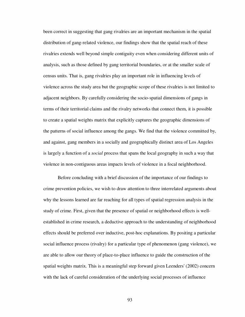
93

been correct in suggesting that gang rivalries are an important mechanism in the spatial

distribution of gang-related violence, our findings show that the spatial reach of these

rivalries extends well beyond simple contiguity even when considering different units of

analysis, such as those defined by gang territorial boundaries, or at the smaller scale of

census units. That is, gang rivalries play an important role in influencing levels of

violence across the study area but the geographic scope of these rivalries is not limited to

adjacent neighbors. By carefully considering the socio-spatial dimensions of gangs in

terms of their territorial claims and the rivalry networks that connect them, it is possible

to create a spatial weights matrix that explicitly captures the geographic dimensions of

the patterns of social influence among the gangs. We find that the violence committed by,

and against, gang members in a socially and geographically distinct area of Los Angeles

is largely a function of a social process that spans the local geography in such a way that

violence in non-contiguous areas impacts levels of violence in a focal neighborhood.

Before concluding with a brief discussion of the importance of our findings to

crime prevention policies, we wish to draw attention to three interrelated arguments about

why the lessons learned are far reaching for all types of spatial regression analysis in the

study of crime. First, given that the presence of spatial or neighborhood effects is well-

established in crime research, a deductive approach to the understanding of neighborhood

effects should be preferred over inductive, post-hoc explanations. By positing a particular

social influence process (rivalry) for a particular type of phenomenon (gang violence), we

are able to allow our theory of place-to-place influence to guide the construction of the

spatial weights matrix. This is a meaningful step forward given Leenders' (2002) concern

with the lack of careful consideration of the underlying social processes of influence

94

exhibited by researchers in their construction of weights matrices. An important corollary

to a deductive approach is that one must carefully match socio-spatial processes to the

specific type of event being studied. For instance, focusing on drug violence might lead

one to specify a weights matrix that captures the important geographical information

pertaining to the location of the markets as well as the spatial dimensions of the actors

involved within the markets. A one-size-fits-all approach to the modeling of spatial

effects of different types of crime is insufficient in a deductive framework, and as Tita

and Greenbaum (2009) noted in their initial work, adapting Leenders’ (2002:26) “change

one’s theory, change W” statement to the current discussion, one is reminded to “change

one’s crime, change W.”

Second, and clearly related to the first, is the need to look beyond measures of

simple contiguity when incorporating spatial effects into models of crime without

necessarily disregarding the underlying spatial structure of a given study area. This

argument takes on added relevance in light of the developing arguments about the

importance of micro-scale units of analysis in criminology (see Weisburd et al. 2009).

Reducing the areal extent of the unit of analysis may also reduce the potential for place-

to-place influence or interaction when modeled through contiguity alone. However, we

are not arguing for throwing out the baby of contiguity with the bathwater. In fact,

contiguity can be an important way to incorporate the overall spatial structure of a study

area, an meaningful goal in the face of likely spillover or other unmeasurable spatial

effects (which may increase as the areal scale of the unit of analysis decreases) (Anselin

1988). Further, contiguity is theoretically justified when exposure is meant to capture

social influence processes wherein local offenders transgress into neighboring areas to

95

commit their crime, or when they influence residents in neighboring areas to carry/use

guns. Our approach to specifying a spatial weights where place-to-place connections can

be defined on both the presence of social network ties and on geographic contiguity

demonstrates that researchers are not faced with an either/or choice and contiguity can be

included with other more-theoretically informed models of place-to-place influence.

Third, conducting an ecological analysis of gang violence presents an interesting

problem with respect to choosing the correct spatial unit of analysis. On the one hand,

researchers have argued that the that the “set space” – the activity space of the gang – can

often only occupy an area as small as a block face, street corner, or perhaps the front yard

of a permissive parent (Whyte 1943; Moore 1991; Klein 1995; Tita et al. 2005). On the

other hand, the territory or “turf” that an individual gang often claims as their domain

may encompass entire neighborhoods. In the Hollenbeck Policing Area there are clearly

examples of both types of gangs. Revisiting Figure 4.5, we see that certain gangs actually

claim different parts of the same relatively small census block groups used in this

analysis. For instance, at the bottom center of the figure we see that Gang 4 and Gang 2

share block group 72 and that Gangs 6 and 22 share geography 8. Gang 22 is a

particularly interesting case as it also claims two of the same block groups as does Gang

12. This suggests, perhaps, that block groups might be too coarsely grained to adequately

capture the activity space of a particular gang or gangs. Alternatively, the gang

prominently displayed in the middle of the figure (Gang 28) is known to occupy space in

fourteen different geographies, sharing none with any other gangs. In this case, one might

argue that block groups are in fact too fine grained a unit of analysis and that these block

groups should be collapsed into a single unit of observation and tied to Gang 28.

96

The above clearly illustrates that researchers interested in understanding the nexus

between the socio-spatial dimensions of urban street gangs and the spatial distribution of

violence must think carefully about the unit of analysis. However, we also recognize that

crime is not simply a function of the socio-spatial dimensions of gangs. Therefore, we

also wanted to be sure to include measures that we believe are theoretically important to

explaining crime (e.g., poverty, residential stability, race/ethnicity, etc.). We chose census

block groups as our unit of analysis for much the same reason that most researchers who

model the ecology of crime do: Census block groups are the smallest unit of geography

for which meaningful data are available. One should also not forget the advice of Hipp

(2007) who reminds us that ultimately there is no “best” unit of analysis and that the

choice of spatial unit of analysis should be driven by empirical and theoretical evidence

which supports the social process matching the spatial scale of analysis. Similar to

Leenders’ (2002:26) advice that “change one’s theory, change W”, Hipp might say

“change one’s social process, change the unit of analysis.”

Lastly, the value of understanding the socio-spatial dimensions of gang rivalries

has important implications for understanding and evaluating geographically targeted

policies. Mears and Bhati (2006) echo this by pointing to the spatial displacement

literature and stating that in addition to considering spatial displacement “there is a

greater need to couple such analysis with theoretically informed assessments about ripple

effects that may occur along geographic and social dimensions” (Mears and Bhati

2006:25). In fact, the evaluation of a gun violence reduction strategy employed in Los

Angeles did just that. The intervention was aimed at reducing the commission of gun

violence by gang members by allocating additional resources (primarily law enforcement,

97

but also social services) in the neighborhoods occupied by specific gangs (Tita et al.

2003). In their evaluation of the effort, the authors demonstrate that in addition to

displacing the benefits of the intervention spatially, the intervention also had the effect of

quelling gun violence among the rivals of the gangs that were targeted for focused

enforcement.

The existence of positive spatial autocorrelation is well supported within the

extant crime and place literature. The value of inductive approaches in terms of positing

various theories and mechanisms responsible for observable patterns of crime cannot be

over-stated. However, after nearly two decades of spatial regression models of crime, it

is time to “un-bound” space and to consider the geographic complexities of mechanisms

of influence such as exposure and/or diffusion. That is, we need spatial models that

adequately capture patterns of social interaction to determine the true geographic

dimensions of influence. The current research has demonstrated the value of employing

such an approach. We were able to posit a mechanism (gang rivalry) and then use

empirical observations to construct an autocorrelation matrix that adequately captured

this mechanism that is so often posited as a major contributor to the clustering of crime in

space. But with the exception of urban street gangs, we know little about the geography

of influence for other types of crimes. It is our hope that others to adopt a deductive

approach to explore other types of violence and crime.

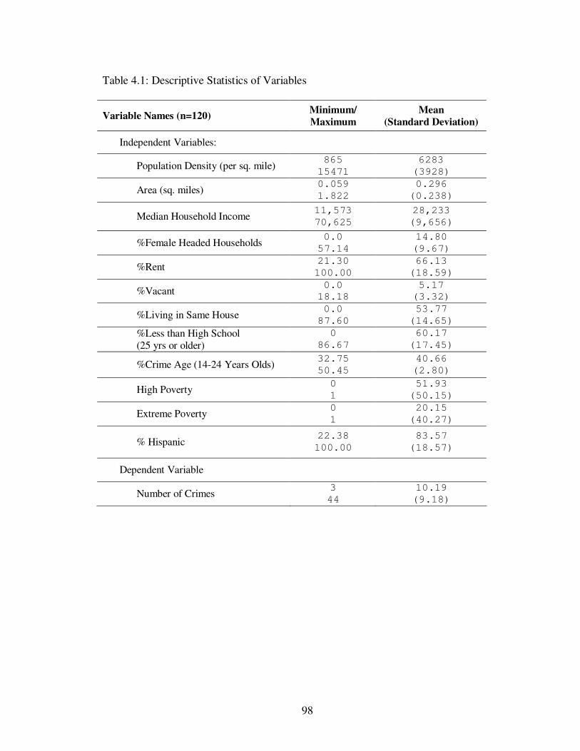
98

Table 4.1: Descriptive Statistics of Variables

Variable Names (n=120) Minimum/

Maximum

Mean

(Standard Deviation)

Independent Variables:

Population Density (per sq. mile) 865

15471

6283

(3928)

Area (sq. miles) 0.059

1.822

0.296

(0.238)

Median Household Income 11,573

70,625

28,233

(9,656)

%Female Headed Households 0.0

57.14

14.80

(9.67)

%Rent 21.30

100.00

66.13

(18.59)

%Vacant 0.0

18.18

5.17

(3.32)

%Living in Same House 0.0

87.60

53.77

(14.65)

%Less than High School (25 yrs or older)

0

86.67

60.17

(17.45)

%Crime Age (14-24 Years Olds) 32.75

50.45

40.66

(2.80)

High Poverty 0

1

51.93

(50.15)

Extreme Poverty 0

1

20.15

(40.27)

% Hispanic 22.38

100.00

83.57

(18.57)

Dependent Variable

Number of Crimes 3

44

10.19

(9.18)

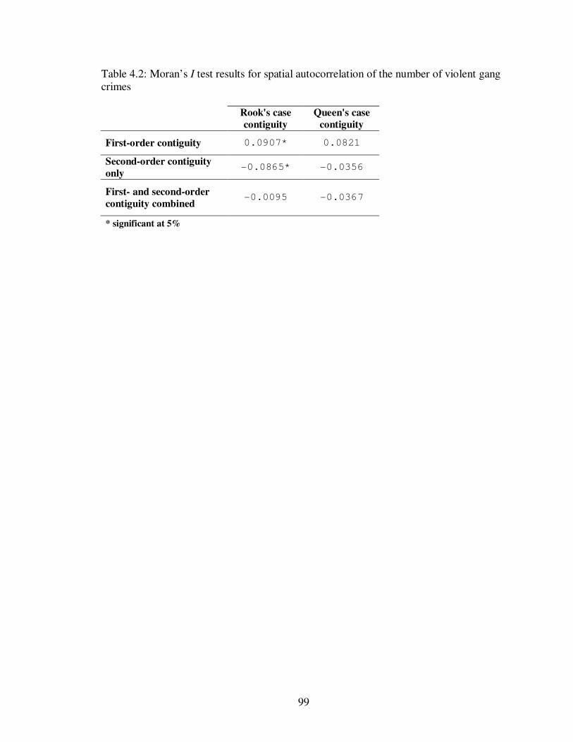
99

Table 4.2: Moran’s I test results for spatial autocorrelation of the number of violent gang crimes

Rook's case

contiguity

Queen's case

contiguity

First-order contiguity 0.0907* 0.0821

Second-order contiguity

only -0.0865* -0.0356

First- and second-order

contiguity combined -0.0095 -0.0367

* significant at 5%

100

Table 4.3: Regression Results (Dependent Variable – Number of Violent Gang Crimes) (1)

Predicting

Crime

(2) Contiguity-based

Lag

(3) Network-based

Lag

(4) Both Lags

Population Density 0.047

(3.27)**

0.036

(0.98)

0.040

(1.19)

0.031

(0.88)

Area (square miles) 0.796

(2.60)**

0.822

(1.43)

1.240

(2.06)*

1.233

(2.06)*

Median Household Income

0.072

(0.89)

0.092

(0.54)

0.132

(0.79)

0.147

(0.76)

%Female Headed Households

2.137

(3.55)**

1.544

(1.16)

1.749

(1.36)

1.486

(1.12)

%Rent -0.015

(4.02)**

-0.017

(2.09)*

-0.012

(1.51)

-0.013

(1.58)

%Vacant -0.019

(0.88)

-0.044

(0.79)

-0.028

(0.59)

-0.038

(0.72)

%Living in Same House

0.001

(0.34)

-0.005

(0.52)

-0.009

(0.94)

-0.012

(1.22)

%Less than High School

0.010

(1.39)

-0.012

(0.49)

-0.000

(0.01)

-0.011

(0.47)

%Crime Age (14-24 Years Olds)

0.003

(0.16)

0.048

(0.75)

-0.015

(0.34)

0.011

(0.18)

Extreme Poverty 0.902

(4.30)**

0.910

(2.05)*

0.971

(2.24)*

0.934

(2.10)*

High Poverty 0.765

(4.88)**

0.876

(2.60)**

0.845

(2.67)**

0.869

(2.61)**

% Hispanic 0.027

(7.79)**

0.022

(2.53)*

0.023

(3.50)**

0.022

(2.82)**

Spatial Lag of Crime 0.186

(1.82)

0.093

(0.87)

Network Lag of Crime

0.085

(2.54)*

0.083

(2.43)*

Constant -0.673

(0.68)

-3.818

(1.00)

-0.480

(0.21)

-2.332

(0.64)

Observations (n=120) Absolute value of z-statistics in parentheses * significant at 5%; ** significant at 1%

101

Table 4.4: J-Test Results

Coefficient Std. Error z P>|z|

Contiguity-based lag 0.059 0.040 1.44 0.151

Network-based lag 0.055 0.016 3.37 0.001

102

Figure 4.1: Map of study site

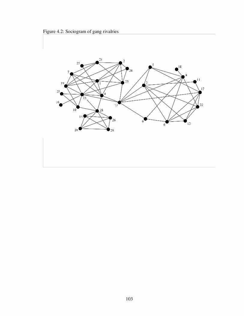
103

Figure 4.2: Sociogram of gang rivalries

104

Figure 4.3: Spatial distribution of violent gang crime

105

Figure 4.4: Network Depiction of the Spatial Contiguity of Hollenbeck

106

Figure 4.5: Gang-by-location network

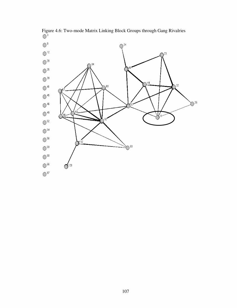
107

Figure 4.6: Two-mode Matrix Linking Block Groups through Gang Rivalries

108

Figure 4.7: Example of the “Structural Equivalence” of Nodes

109

CHAPTER 5

SPATIALIZING SOCIAL NETWORKS: GEOGRAPHIES OF RIVALRY,

TERRITORIALITY, AND VIOLENCE

This chapter, published in the Annals of the Association of American Geographers

(Radil et al. 2010), blends concepts and techniques from social network analysis with

conventional spatial analysis to theorize the socio-spatial processes involved in the

‘hybrid’ weights matrix from the previous chapter and to perform an analysis of the

spatial patterning of violence using a social network analysis methodology. This research

finds evidence for the production of differential spaces of violence in Hollenbeck, which

I interpret as partial evidence of the social production of space, which is simultaneously

made by the actions of the gangs and a mediator of further action by the gangs

themselves. This paper is presented in this chapter unaltered from the published version

aside from minor formatting changes.

INTRODUCTION

Social network analysis is an increasingly prominent technique in a number of

social sciences and seemingly has obvious connections to geographies of networks and

flows that have become popular in studies of globalization as well as identity politics

(Murdoch and Marsden 1995; Dicken et al. 2001; Lantham 2002; Sheppard 2002).

However, the compatibility of the techniques of social network analysis to geographic

theories of networks has been challenged because of a lack of geographic nuance or

consideration of the spatialities of power and other social relations in social networks

(Allen 2003; Bosco 2006a). We recognize these shortcomings and explore the technique

of structural equivalence in social networks as a means to incorporate theoretically

110

informed geographies of situation or embeddedness into social network analysis, a

specific step in the broader project of integrating social theories of geography and spatial

analytical techniques (Goodchild et al. 2000).

Specifically, we explore how an actor’s position in geographic space can be

analyzed simultaneously with their position in social networks. The geographic premise

that social behavior is context-specific, and that space and society are mutually

constituted, requires the incorporation of multiple spatialities into the analysis of social

processes (Leitner et al. 2008). A typical social network analysis is a one-dimensional

spatiality, identifying an actor’s location in a social network. By spatializing social

networks to include actors’ simultaneous position in networks of relations and places we

offer a technique to analyze the simultaneous embeddedness of actors in both network

space and geographic space. The term embeddedness has become popular in discussing

social networks to illustrate the many situations that social actors create and must

negotiate in their behavior (Bosco 2006b). Embeddedness may be seen as a process of

creating an increasing intensity of relationships (Bosco 2006b), but it is also a recognition

that relationships, distance, and place-specific social relations are intertwined to situate

actors (Sheppard 2002; Ettlinger 2003; Staeheli 2003; Leitner et al. 2008). Spatializing

social networks facilitates the analysis of social behavior within the simultaneous and

related contexts of network position and relative location in geographic space.

The ability of spatial analysis to incorporate the relative location of social actors,

and the linkages between them, can, paradoxically, atomize actors being studied through

a “spatial fetishism” that ignores or is unable to address the social relations that construct

111

the spaces within which actors operate.23 Simply put, spatial analysis is good at analyzing

clusters of social behaviors and phenomena (such as crime or disease) but struggles to

illustrate the underlying causal structures and relationships. When spatial analysis is

overly dependent on reasoning from spatial form to social process, the risk of reducing

people to the spaces they occupy grows while the likelihood for new insights shrinks. A

spatial analysis that is grounded in theories of the social construction of space and that

can model the spatial patterning of relevant social relationships would represent a

meaningful advance.

We argue that such an outcome is possible through making use of the concept of

embeddedness and the related social network analytic technique of structural

equivalence. By performing a hybrid analysis that integrates a spatial analytic approach

into the analysis of social networks, we believe that we make a first useful step towards

spatializing social network analysis while reducing the possibility of privileging space

over social process. The technique we outline combines relative position in geographic

space with social network position in a manner that identifies similarly situated actors in

network and geographic spaces simultaneously. This in turn allows hypothesis

development and evaluations of how differences in position in multidimensional

spatialities may be said to relate to material outcomes. The technique and its ability to

inform are illustrated by an analysis of gang violence in Los Angeles.24

23 This critique can be traced to Wolpert’s (1964) behaviorist approach, but saw a more recent manifestation in Harley’s (1989) critiques of the cultural norms within cartographic representations and Pickles’ (1995) concerns of the unacknowledged representations in GIS. More recently Bosco (2006a) and Ettlinger and Bosco (2004) have noted the need to consider power relations in social network analysis. See also Collinge (2005: 191-201) for a contemporary discussion of spatial fetishism. 24 This paper reports on initial findings in a collaborative project between geographers and a criminologist and extends the results of an exploratory spatial analysis of gang violence by the criminologist (Tita et al. 2003). The data used in this paper are the same as used in Tita et al. (2003).

112

In the following section, a discussion of embeddedness and how it relates to

network perspectives and methods is offered. We then describe the study area and

introduce the data used: a social network of gang rivalries and the geographic distribution

of gang-related violence in the Hollenbeck Policing Area in Los Angeles, CA. We

theorize territoriality, geographic embeddedness, and network position as the specific

spatialities at work in the rivalry network and discuss how to consider these

simultaneously. In the subsequent section, we present the results of a multi-relational

positional analysis using social network methods. We conclude the paper with a

discussion of the findings, which demonstrate that the spatialized social network is

indeed a useful lens on gang violence in Hollenbeck. The geographic patterns in

measures of violence in Hollenbeck are interpretable through and clarified by an

understanding of the both the network and spatial relationships of the rivalry relations

between gangs in the area. The technique demonstrated here has promise beyond this one

study of gang crime. It operationalizes relational data in a way that allows simultaneous

systematic evaluation of the way in which social actors’ positionality in network

relationships and spatial settings provide constraints and possibilities upon their behavior.

In the conclusion we briefly explore how this technique can be further developed to allow

for the addition of other spatialities into a systematic analysis.

EMBEDDEDNESS, SPATIAL ANALYSIS, AND SOCIAL NETWORK ANALYSIS

One particular way in which geographers have tried to understand the behavior of

social actors (individuals, groups, organizations, or other social collectives) situated in

specific contexts is through the concept of embeddedness. As noted by Ettlinger (2003),

113

Hess (2004) and others, the use of embeddedness in geography largely arose from the

work of sociologist Mark Granovetter. In a parallel to calls for more ‘spatialized’ social

science approaches (e.g., Goodchild et al. 2000), Granovetter (1985) argued for a more

‘socialized’ understanding of “the extent to which economic action is embedded in

structures of social relations,” and described what he called the argument of

embeddedness: “that the behavior and institutions to be analyzed are so constrained by

ongoing social relations that to construe them as independent is a grievous

misunderstanding” (1985: 481–482). This idea of embeddedness as a form of structural

constraint on social action made use of a reading of the word embed that implies a state

of being surrounded tightly, enveloped, or otherwise constrained. However, another

reading of the word embed suggests not just closeness but the state of something

becoming part of an integral whole. Later Granovetter (1992) refined his arguments to

differentiate between the kind of embeddedness that suggests closeness (which he called

‘relational embeddedness’) and the kind that suggests the importance of position in a

larger whole (‘structural embeddedness’).

Both perspectives on embeddedness have been important for geography.

Embeddedness as closeness has resonance for geographers that explore the themes of

geography, space, and place as contexts with implications for human behavior. Entrikin

offers a helpful example with the claim that “my life is always embedded in the story of

those communities from which I derive my identity’’ (1991: 9). For Entrikin, the

‘embeddedness’ of being within a place-specific social milieu is inseparable from the

particulars of human activity. Entrikin’s sentiments also reflect Pred’s (1984) theoretical

understanding of place as a historically contingent process. Embeddedness as position in

114

a larger social structure is also an emerging theme. For example, Flint argued that space

is partly produced by the “connections [of a given place] to the rest of the world” (2002,

33) and that, presumably, different connections lie at the heart of the production of

different kinds of spaces. In fact, as Staeheli (2003) points out, this perspective on space

blurs with concepts of place in geography. Although space has historically been

understood as referencing the general or universal in geography, as Staeheli notes,

contemporary concepts of the social construction of space leads to a refocus from the

universality of processes across space to the unique outcomes present in different spaces:

spaces become ‘social locations’ embedded in “webs of cultural, social, economic, and

political relationships” (Staeheli 2003: 160). From this perspective, the distinctiveness of

spaces/places is due to the ‘embeddedness’ of being differently located in larger social

structures.

As Granovetter (1992) suggests, these different perspectives on embeddedness are

not mutually exclusive or necessarily discrete categories, but rather points that blend into

the other. As such, both may be seen as important elements in geographic arguments

about the social production of space and how geography mediates social behavior in

places. For example, when Agnew (1987) described places as composed of three related

elements (locale, location, and sense of place), embeddedness as closeness is similar to

Agnew’s description of locale as “the settings in which social relations are constituted,”

while embeddedness as position is similar to Agnew’s notion of location as “the

geographical area encompassing the settings for social interaction . . . at a wider scale”

(1987: 28). Massey (1993: 66) provides another useful example: her power-geometry

concept is concerned with the position of individuals and social groups relative to the

115

spatial flows of people, information, and capital between places while her progressive

sense of place concept incorporates both kinds of embeddedness, emphasizing the role of

social relations that are both “in a situation of co-presence” and “stretched out over

space.” Drawing on these lines of thinking, social behavior can be understood as affected

and produced not just by the specific embedded practices, conditions, institutions, or

identities of a single place, social location, space, or geography, but also by the way these

features are in turn affected and produced by the specific embedded practices, conditions,

institutions, or identities of other places, social locations, spaces, or geographies to which

they are connected.

Many kinds of spatial analysis make use of the concept of embeddedness as

closeness. For example, spatial econometric models consider the influence of places on

each other by formalizing the geographic connectivity between the units of analysis

which is used to create new variables for inclusion into statistical models (Anselin 2002).

More plainly, the degree to which a focal spatial unit is embedded in its closest

neighboring geographies is modeled, usually either by identifying its areal contiguity

with other spatial units or by selecting neighbors based on the smallest geographic

distances between them. Beyond the issues of spatial fetishism, there are some

meaningful limitations to this particular approach. All the processes that might contribute

to the production of certain spatial patterns are modeled in the same fashion — by using

the relative location of each unit of analysis. For example, in an analysis of U.S. crime

patterns aggregated to the scale of counties, Baller et al. (2001) accounted for all the

processes of social interaction between counties by defining a set number of the nearest

counties (measured by the geographic distance between the approximate center of each

116

county) as influential neighbors for a given focal county. Then, crime data from the set of

influential neighbors were used to create a “spatial lag” variable that was included with

other explanatory variables for regression modeling (Baller et al. 2001).

In this example, embeddedness is simply the degree to which each county exhibits

similarity in crime and location. If the social relationships that are theorized to underlie a

particular observed geographic form are one of embeddedness as closeness, then the

model used by Baller and his colleagues may be an appropriate choice. What this

approach does not allow is a consideration of any spatiality that cannot or should not be

operationalized through an examination of the qualities of the closest units in geographic

space. This limitation is meaningful because as observed by Leitner et al. (2008),

multiple spatialities are bound up in issues of interest to geographers and these should be

examined together where possible. Ettlinger (2003: 161) emphasized similar themes

when describing what she refers to as overlapping networks: “the intersection of different

networks in which individuals are engaged,” where each network may be thought to

represent different kinds of relationships and where only some relationships are “based

on proximity.” Kwan (2007) also argues that the complexity of human spatial behavior

cannot be captured in spatial models with a single type of spatial measurement, such as

distance. Quantitative analytic techniques that allow for the consideration of more than a

single kind of embeddedness, including position within a social network, would be an

important step in addressing the concerns noted above.

Embeddedness that is based upon occupying a particular position within a

network is a central concept within sociology. Since the work of Georg Simmel (Simmel

1955: see also Breiger 1974 and Grabher 2008) in the late 19th and early 20th centuries

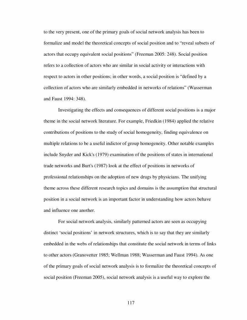
117

to the very present, one of the primary goals of social network analysis has been to

formalize and model the theoretical concepts of social position and to “reveal subsets of

actors that occupy equivalent social positions” (Freeman 2005: 248). Social position

refers to a collection of actors who are similar in social activity or interactions with

respect to actors in other positions; in other words, a social position is “defined by a

collection of actors who are similarly embedded in networks of relations” (Wasserman

and Faust 1994: 348).

Investigating the effects and consequences of different social positions is a major

theme in the social network literature. For example, Friedkin (1984) applied the relative

contributions of positions to the study of social homogeneity, finding equivalence on

multiple relations to be a useful indictor of group homogeneity. Other notable examples

include Snyder and Kick's (1979) examination of the positions of states in international

trade networks and Burt's (1987) look at the effect of positions in networks of

professional relationships on the adoption of new drugs by physicians. The unifying

theme across these different research topics and domains is the assumption that structural

position in a social network is an important factor in understanding how actors behave

and influence one another.

For social network analysis, similarly patterned actors are seen as occupying

distinct ‘social positions’ in network structures, which is to say that they are similarly

embedded in the webs of relationships that constitute the social network in terms of links

to other actors (Granovetter 1985; Wellman 1988; Wasserman and Faust 1994). As one

of the primary goals of social network analysis is to formalize the theoretical concepts of

social position (Freeman 2005), social network analysis is a useful way to explore the

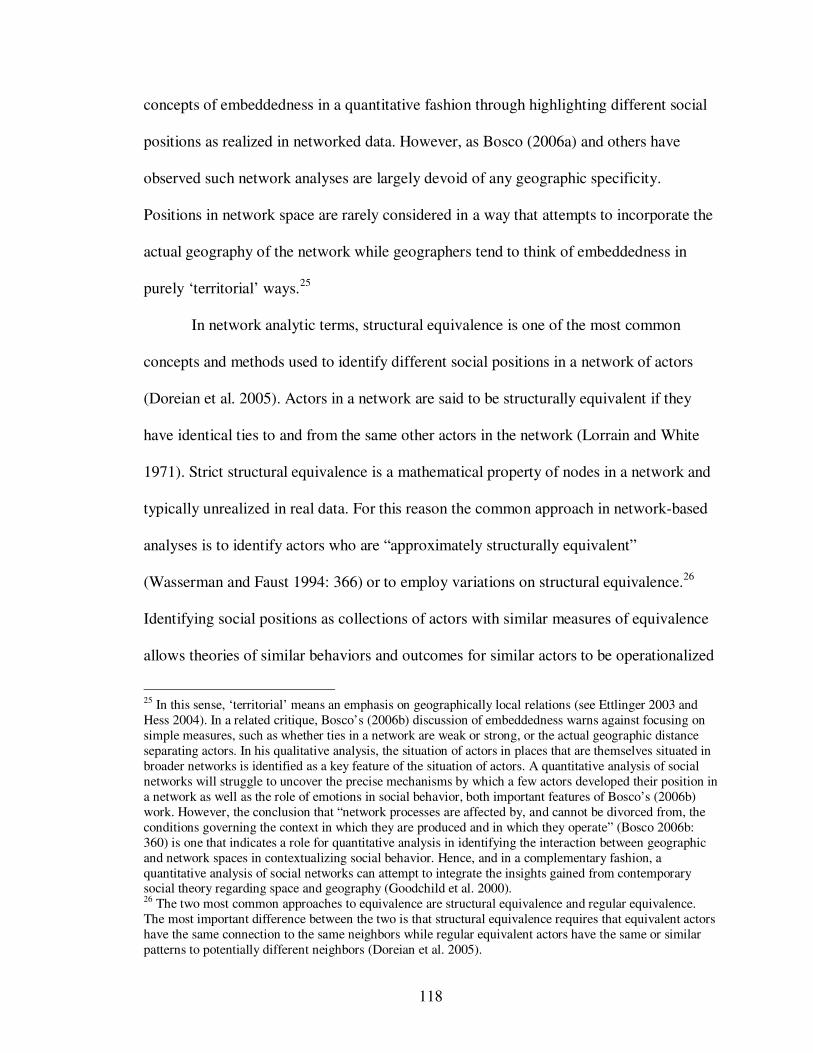
118

concepts of embeddedness in a quantitative fashion through highlighting different social

positions as realized in networked data. However, as Bosco (2006a) and others have

observed such network analyses are largely devoid of any geographic specificity.

Positions in network space are rarely considered in a way that attempts to incorporate the

actual geography of the network while geographers tend to think of embeddedness in

purely ‘territorial’ ways.25

In network analytic terms, structural equivalence is one of the most common

concepts and methods used to identify different social positions in a network of actors

(Doreian et al. 2005). Actors in a network are said to be structurally equivalent if they

have identical ties to and from the same other actors in the network (Lorrain and White

1971). Strict structural equivalence is a mathematical property of nodes in a network and

typically unrealized in real data. For this reason the common approach in network-based

analyses is to identify actors who are “approximately structurally equivalent”

(Wasserman and Faust 1994: 366) or to employ variations on structural equivalence.26

Identifying social positions as collections of actors with similar measures of equivalence

allows theories of similar behaviors and outcomes for similar actors to be operationalized

25 In this sense, ‘territorial’ means an emphasis on geographically local relations (see Ettlinger 2003 and Hess 2004). In a related critique, Bosco’s (2006b) discussion of embeddedness warns against focusing on simple measures, such as whether ties in a network are weak or strong, or the actual geographic distance separating actors. In his qualitative analysis, the situation of actors in places that are themselves situated in broader networks is identified as a key feature of the situation of actors. A quantitative analysis of social networks will struggle to uncover the precise mechanisms by which a few actors developed their position in a network as well as the role of emotions in social behavior, both important features of Bosco’s (2006b) work. However, the conclusion that “network processes are affected by, and cannot be divorced from, the conditions governing the context in which they are produced and in which they operate” (Bosco 2006b: 360) is one that indicates a role for quantitative analysis in identifying the interaction between geographic and network spaces in contextualizing social behavior. Hence, and in a complementary fashion, a quantitative analysis of social networks can attempt to integrate the insights gained from contemporary social theory regarding space and geography (Goodchild et al. 2000). 26 The two most common approaches to equivalence are structural equivalence and regular equivalence. The most important difference between the two is that structural equivalence requires that equivalent actors have the same connection to the same neighbors while regular equivalent actors have the same or similar patterns to potentially different neighbors (Doreian et al. 2005).

119

and tested. These sorts of questions are drawn from theories of social influence which

generally posit that identically positioned actors in a relational network use each other as

a frame of reference for appropriate behavior even if the actors have no direct interaction

with the other (Burt 1987: 1293). From this perspective, influence is directly tied to the

perception of what constitutes proper actions for actors in specific network positions

(Galaskiewicz and Burt 1991).

Network-based operationalizations of theories of social position offer potential

insight into the spatiality of social behavior. We begin with the recognition that space is

socially constructed, and emphasize that part of the construction process relates to the

simultaneous geographic embeddedness and network position of actors. Conceptualizing

the geographic spaces within which actors are embedded as a kind of relational network

and using the ability of network methods to identify similarly positioned actors can lead

to a consideration of the spatiality of these networks. In other words, combining

geographic and social networks in such a way that identifies differently structured spaces

(beyond just a consideration of the relative location of these spaces) may offer insight

into the relational nature of space and how measures of equivalence relate to specific

behavioral outcomes in different spaces of social position.

We call this approach spatializing social networks. As an analytic framework, this

approach allows influence to take place not just between geographically proximate

neighbors (as with conventional spatial analysis) but also between actors that are close in

terms of social network space. We see this as a first step toward addressing the complex

nature of embeddedness (Bosco 2006b) and considering more than one spatiality of

embeddedness (Leitner et al. 2008). Spatializing social networks allows the identification

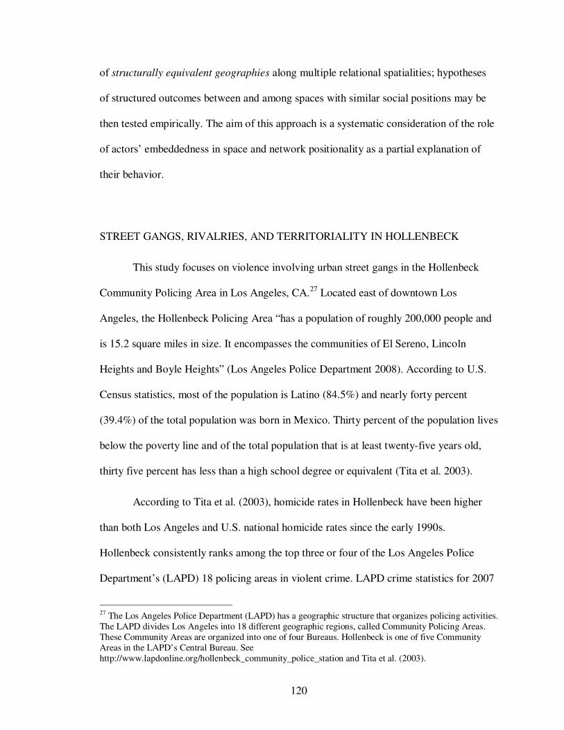
120

of structurally equivalent geographies along multiple relational spatialities; hypotheses

of structured outcomes between and among spaces with similar social positions may be

then tested empirically. The aim of this approach is a systematic consideration of the role

of actors’ embeddedness in space and network positionality as a partial explanation of

their behavior.

STREET GANGS, RIVALRIES, AND TERRITORIALITY IN HOLLENBECK

This study focuses on violence involving urban street gangs in the Hollenbeck

Community Policing Area in Los Angeles, CA.27 Located east of downtown Los

Angeles, the Hollenbeck Policing Area “has a population of roughly 200,000 people and

is 15.2 square miles in size. It encompasses the communities of El Sereno, Lincoln

Heights and Boyle Heights” (Los Angeles Police Department 2008). According to U.S.

Census statistics, most of the population is Latino (84.5%) and nearly forty percent

(39.4%) of the total population was born in Mexico. Thirty percent of the population lives

below the poverty line and of the total population that is at least twenty-five years old,

thirty five percent has less than a high school degree or equivalent (Tita et al. 2003).

According to Tita et al. (2003), homicide rates in Hollenbeck have been higher

than both Los Angeles and U.S. national homicide rates since the early 1990s.

Hollenbeck consistently ranks among the top three or four of the Los Angeles Police

Department’s (LAPD) 18 policing areas in violent crime. LAPD crime statistics for 2007

27 The Los Angeles Police Department (LAPD) has a geographic structure that organizes policing activities. The LAPD divides Los Angeles into 18 different geographic regions, called Community Policing Areas. These Community Areas are organized into one of four Bureaus. Hollenbeck is one of five Community Areas in the LAPD’s Central Bureau. See http://www.lapdonline.org/hollenbeck_community_police_station and Tita et al. (2003).

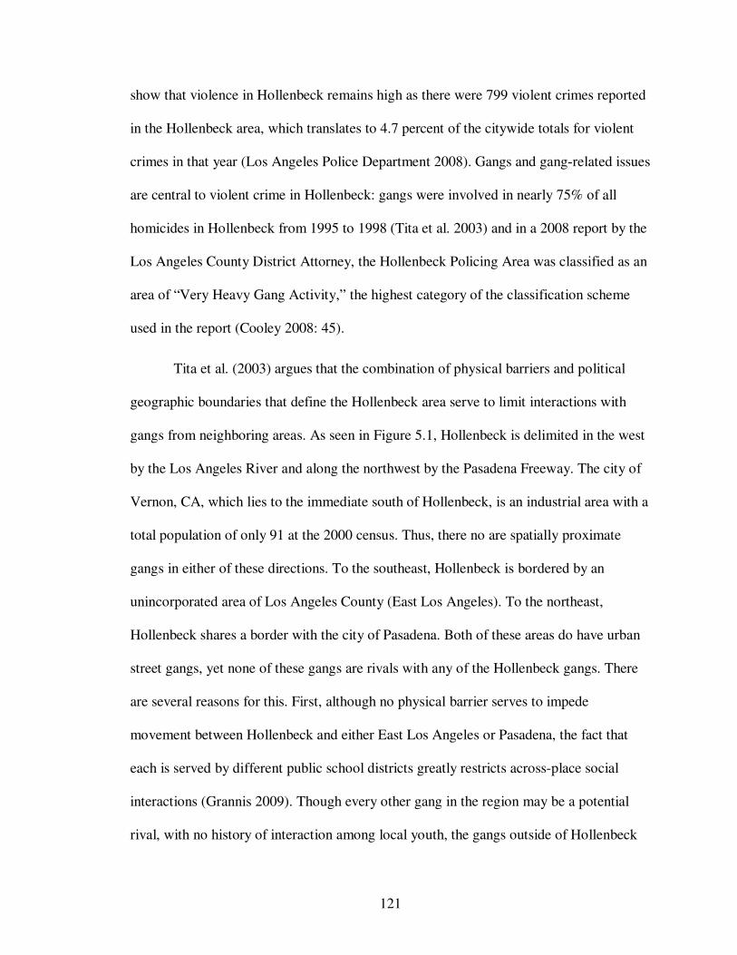
121

show that violence in Hollenbeck remains high as there were 799 violent crimes reported

in the Hollenbeck area, which translates to 4.7 percent of the citywide totals for violent

crimes in that year (Los Angeles Police Department 2008). Gangs and gang-related issues

are central to violent crime in Hollenbeck: gangs were involved in nearly 75% of all

homicides in Hollenbeck from 1995 to 1998 (Tita et al. 2003) and in a 2008 report by the

Los Angeles County District Attorney, the Hollenbeck Policing Area was classified as an

area of “Very Heavy Gang Activity,” the highest category of the classification scheme

used in the report (Cooley 2008: 45).

Tita et al. (2003) argues that the combination of physical barriers and political

geographic boundaries that define the Hollenbeck area serve to limit interactions with

gangs from neighboring areas. As seen in Figure 5.1, Hollenbeck is delimited in the west

by the Los Angeles River and along the northwest by the Pasadena Freeway. The city of

Vernon, CA, which lies to the immediate south of Hollenbeck, is an industrial area with a

total population of only 91 at the 2000 census. Thus, there no are spatially proximate

gangs in either of these directions. To the southeast, Hollenbeck is bordered by an

unincorporated area of Los Angeles County (East Los Angeles). To the northeast,

Hollenbeck shares a border with the city of Pasadena. Both of these areas do have urban

street gangs, yet none of these gangs are rivals with any of the Hollenbeck gangs. There

are several reasons for this. First, although no physical barrier serves to impede

movement between Hollenbeck and either East Los Angeles or Pasadena, the fact that

each is served by different public school districts greatly restricts across-place social

interactions (Grannis 2009). Though every other gang in the region may be a potential

rival, with no history of interaction among local youth, the gangs outside of Hollenbeck

122

remain outside of the awareness space of the Hollenbeck gangs. Second, there exists a

simple propinquity effect as none of the gangs found in either East Los Angeles or

Pasadena occupy space on the border shared with Hollenbeck. The net effect of these

border features, both physical and political, is to create a landscape within which the

rivalries of the Hollenbeck gangs are wholly contained (Tita et al. 2003).

Hollenbeck is no stranger to gangs and gang activity. The history of urban street

gangs in east Los Angeles, including Hollenbeck, is a long one, with some gangs

documented back to the late 1940s (Moore 1991). From 2000 to 2002, 29 active gangs

were identified in the Hollenbeck area (Tita et al. 2003). Control over territory is a central

theme for the gangs of Hollenbeck. The gangs in Hollenbeck are what Klein (1995)

describes as ‘traditional’ in that they have a strong attachment to turf, or the territory

under the direct control of a gang. Tita et al. (2003) makes a similar argument and

characterizes the gang violence in Hollenbeck as expressly tied to the defense of turf and

control over territory. Although they arise from different motivations, the anti-gang

activities of the LAPD also revolve around control of territorial space. As described by

Herbert (1997) “police (LAPD) strategies to create public order involve enacting

boundaries and restricting access” (1997: 11). The key point here, made by Sack (1986)

and others (e.g., Paasi 2003), is that territory is not the static result of social processes but

is instead what Newman calls an “imperative” and an “essential component of human

behavior” (2006: 88-89). The attempts by the various gangs to control the spaces of

Hollenbeck result in violence between the different street gangs themselves.

Understanding the spatial patterning of the relationships between the gangs, themselves

123

wrapped up in issues of contesting and controlling space, are key to understanding the

spatial patterning of gang violence in Hollenbeck.

The emphasis on territorial control by gangs in Hollenbeck relates to a key way in

which spaces and places are socially constituted. In geography, territoriality is often seen

as the “delimitation of boundaries” and the interrelated “behavior within those

boundaries” (Kahler 2006: 2). Robert Sack’s (1986) influential work on territoriality

defines it as the use of territory for political, social, and economic ends and it has been

most often associated with the spatiality of the nation-state (Paasi 2003). We can say that

territoriality is conventionally understood in geography as involving both a partitioning

of space into distinct units and ongoing attempts to control the space in order to maintain

the borders between the units (Kuus and Agnew 2008). These characteristics track well

with how Tita describes gang turf: a well-defined geographic area of a city, such as a

neighborhood, that is claimed by the gang as its ‘domain’ (Tita et al. 2005).

Territoriality as domain and partitioning behavior leads Newman (2006: 91) to

conclude that territorial behavior is quite meaningful at “local levels”: “rivalries are

played out through the daily life practices of segregated groups residing in their own

distinct . . . neighborhood turfs.” Both Newman's (2006) emphasis on spatial segregation

and Cresswell's (1996) work on places as geographic expressions of cultural norms and

transgression to those norms suggests a reason why the persistent territoriality of

Hollenbeck's various gangs might result in violence between them. When a gang member

enters the turf another gang, a spatial transgression has occurred and the gang member is

now “out of place.” In these situations, the response to such spatial transgressions may

involve violence. If presence in other turfs can be seen as transgressive, there is an

124

expectation that local geographic embeddedness or the relative nearness to differently

controlled spaces is an important element to certain kinds of outcomes, such as violence

(Kahler 2006).

MAPPING GANG VIOLENCE IN HOLLENBECK

As described in Tita (2006), from 2000-2002, Hollenbeck experienced 1,223 violent

crimes by or against gang members. This kind of violence is defined by Tita (2006) as ‘gang

related’ and includes the protection of turf from an incursion by rival members as well as all

other violence involving a gang member. The list of crimes over this time period include the

legal classifications of aggravated assaults, simple assaults, assault with a deadly weapon,

attempted homicides, homicides, robberies, kidnappings, and firing a gun into an inhabited

dwelling/vehicle.28 When aggregated by U.S. Census block groups, mapping the violent

crimes suggest two important features (see Figure 5.2). First, violence has penetrated all

areas of Hollenbeck and, second, there may be some spatial clustering of gang-related

violence.

The first point is straightforward as violent crimes were present in every block group.

Incident counts by block group range from a low of 1 (occurring 6 times) to a high of 44

(occurring once) with a mean across block groups of 10.19. To evaluate the second

observation, a global Moran’s I test of spatial autocorrelation was performed by identifying

block groups as neighbors on the basis of either sharing a common length of border (“rook”

28 Rape and domestic violence reports were not available and not included in violence counts (Tita et al. 2003).

125

contiguity) or sharing a single border point (“queen” contiguity).29 Despite the presentation

in Figure 5.2, neither rook nor queen configurations resulted in strong statistical measures of

dependence (see Table 5.1). The Moran’s I ratios of 0.09 for rook and 0.08 for queen are

interpreted as very weak positive dependence (positive dependence means neighboring

values are similar). In fact repeating the test by increasing the contiguity from first-order

neighbors (those that share border lengths or points) to also include second-order neighbors

(neighbors of the first set of neighbors using the same criteria of shared border length or

point) results in measures that are interpreted as very weak negative spatial dependence

(neighboring values are dissimilar; Moran’s I ratio’s of -0.09 for 2nd order rook and -0.04 for

2nd order queen). While the absence of evidence for robust global spatial dependence may be

due to the level of aggregation in the data, it also does not recommend a conventional spatial

analytic approach.

GANG RIVALRY AND TERRITORIAL NETWORKS

Tita et al.’s (2003) analysis of violence pertaining to the 29 different gangs active

in Hollenbeck from 2000-2002 identified a social network of gang rivalries. Rivalry is a

meaningful relation in this circumstance as urban street gangs are committed to the

defense of their turf and have negative relationships (i.e., rivalries) that explicitly tie them

to other gangs (Tita et al. 2003). This interpretation is related to implications of rivalries

as a key social relation in the attempt to understand other forms of violence (see Diehl

and Goertz 2000 and Flint et al. 2009 for examples). The rivalry relations were identified

through the use of a survey by Tita et al. (2003) that asked informants from both the

29 Contiguity matrices and Moran’s I tests were constructed and performed using the GeoDa spatial econometric software package (Anselin et al. 2006).

126

LAPD and some of the gangs to identify the rivalries between each of the gangs.30 A

network diagram of these rivalries is shown in Figure 5.3. The nodes in this network

represent the gangs and the connections between them represent the rivalries. The

measurement of rivalry was binary where the presence of a rivalry resulted in a link and

the absence of a rivalry resulted in no link. Every gang was connected to the network

structure and the number of rivalries ranged from a minimum of 1 to a maximum of 10.

As is common in network analyses, the network can also be described as a matrix. In this

case, a 2929× binary matrix was produced where the presence of a rivalry between the

gangs was coded as 1 and the absence of a rivalry was coded as 0 (Tita et al. 2003).

In addition to identifying gang rivalries, the location and boundaries of the turf of

each of the 29 gangs was mapped through the participation of the LAPD (Tita et al.

2003). Tita (2006) later used U.S. Census block group areal units to establish the

presence or absence of gang turf at a geographic level that possessed data of interest to

ecological studies of crime. The Hollenbeck area is comprised of 120 such block groups

and gang turf was present in 103 of these units. In seven instances, more than one gang

claimed turf in the same block group. However, close spatial proximity was not always a

predictor of rivalry (Tita 2006).

After identifying both a social network of rivalries and the relative geographic

locations of gang turf with a disaggregated territorial map, Tita (2006) made a unique

methodological choice by attempting to blend these structures together. This was done by

30 Rivalry relationships between the gangs were identified through the use of a survey of local police and former gang members by Tita et al. (2003). Each informant was provided with a survey comprised of one page for each gang. At the top of the page, a particular gang was identified and the respondent was asked to ‘Please Identify All of the Gangs that are an Enemy of the <insert gang name>.’ Law enforcement experts and several current and former gang members completed the survey and there was perfect agreement across the gang members’ and law enforcement experts’ surveys.

127

first reimagining the geography of gang turf as a network of neighbors, a conventional

way to produce a 'spatial weights matrix' for use in spatial econometric models (Anselin

2002). Each areal unit of Hollenbeck (census block groups) became a single node in a

new network and the links between the nodes were based on geographic contiguity. The

coding scheme was again binary where block groups that shared borders are formally

connected while those that do not remained unconnected. After distributing the gang

rivalries to the disaggregated territorial map, the two separate network matrices

( 2929× gang rivalries and 120120× census block groups) were then associated using

matrix multiplication to produce a single 120120× matrix for use in a spatial

econometric model. This weights matrix was then used to create a new explanatory

variable, which was included in a regression along with a variety of other common

measures in criminology, such as education and income (Tita 2006).

Tita's (2006) use of the hybrid weights matrix as the connectivity input for a

spatial econometric regression model was an innovative approach in the spatial

econometric modeling of crime, but it also kept at arm's length one of the central claims

of relational social science - that relationships between actors have more explanatory

power than do attribute-based categories (Emirbayer and Goodwin 1994; Emirbayer

1997). Despite using relational data (the relative locations of the gangs and the rivalry

relationships), the initial analytic product was another attribute-based explanatory

variable and the analytic focus remained on the perceived causal power of attributes.

Additionally, and most importantly for this paper, this approach forced network position

to be modeled as local geographic embeddedness. In other words, the theoretically

distinct spatialities of embeddedness were operationalized as a single form of

128

embeddedness and all interactions between the geographic units of analysis became

overly ‘territorialized’ (Hess 2004).

The lack of fidelity to the explanatory power of relationships along with the fact

that both the spatialities of geographic embeddedness and network positionality must be

operationalized in the same way leaves something to be desired. On this basis and by

drawing on Anselin's (2002) observation that the construction of the spatial weights

matrix in spatial econometric models is actually based on social network concepts, the

authors began a series of conversations that extended Tita’s previous analysis while

engaging theoretical discussions of embeddedness. In this paper, the particular outcome

is a consideration of whether structural similarity based on both kinds of embeddedness

contributes to similar outcomes for actors.31 We examine this question in a way that that

fits the spatialities under consideration. The hypothesis here is whether or not similarly

embedded and positioned territorial spaces experience similar amounts of violence. In

other words, can structurally equivalent geographies be identified from both the

embedded gang turf and the rivalry network that connects them and do differently

structured geographies exhibit different violence patterns?

SPATIALIZING THE SOCIAL NETWORKS OF HOLLENBECK’S GANG

RIVALRIES

Positional analyses involve identifying social positions in a relational network

based on similar patterns of links between individual nodes. The process is well

31 See Leenders (2002) for a discussion of the nature of the spatial weights matrices in spatial econometrics and similarities with social network analysis.

129

developed in social network analysis and most positional analyses “focus on identifying

subsets of equivalent actors” (Wasserman and Faust 1994: 354). Identifying subsets in a

complex network involves simplifying the networked data. Whether presented as a

network diagram or a matrix, it is difficult to visually identify meaningful patterns that

may exist. For example, the spatialized rivalry network is shown in Figure 5.4. The

complexity of the ties precludes visual interpretation. However, a matrix of spatialized

rivalry relations may be reorganized on the basis of similar ties between actors in the

network. This activity is referred to in network terms as matrix permutation and allows

similar actors to be grouped together (Wasserman and Faust 1994).

As previously discussed, relationships between the 29 different gangs of

Hollenbeck may be represented in matrix form. However, the rows and columns of the

resulting 2929× matrix represent both a social unit (gangs) and a territorial unit (turf).

As such, there are two distinct spatialities of embeddedness that must be considered: local

geographic embeddedness and position in the overall network structure. Geographic

embeddedness, especially among territorial units with demarked boundaries and that are

mutually exclusive of other units (such as gang turf), can be represented in the

conventional spatial econometric way through a consideration of relative location.

Neighboring gang turf (those that comprise the geography in which a given gang's turf is

embedded) can be identified through shared borders. The rivalry network can be

represented in a similar way, with rivalries between gangs coded in the matrix. The result

is two 2929× matrices, one for each spatiality.

While the 2929× matrices capture all the social and territorial units identified by

Tita et al. (2003) in the Hollenbeck Policing Area, the matrices do not capture the entire

130

geography of Hollenbeck. There are areas of Hollenbeck that are not claimed as turf by

any of the gangs but that do experience gang-related violence. Although these areas of

Hollenbeck do not represent the territorial claims of the gangs, we include these areas

into both the geographic embeddedness matrix and the network positionality matrix. An

important reason for this choice is that some of the gangs do not share borders with other

gangs and are instead bounded by unclaimed areas. However, these unclaimed areas still

must be negotiated in some sense to reach the turf of other gangs and therefore may be

understood as a kind of connective tissue to the overall gang geography (see Tita and

Cohen 2004: 199). Further, as an empirical reality, gang-related violence is not wholly

contained within claimed turf and excluding unclaimed areas would also involve

excluding information that could affect the outcome of the analysis. More plainly, a

consideration of local geographic embeddedness that did not include unclaimed spaces

would be partial and incomplete. For these reasons, the unclaimed areas were included by

simply adding another row and column to each matrix. In the case of the geographic

embeddedness matrix, the unclaimed areas were treated as another possible neighbor in

the embedded geography of the gang turf. For the network positionality matrix, the

unclaimed areas never resulted in a link as they did not represent a social unit that another

gang could have a rivalry with. The final result was two binary 3030× matrices.

The identification of equivalent geographies on the patterning of ties of both

geographic embeddedness and network positionality was accomplished using the network

analysis program UCINET (Borgatti et al. 2005). The particular technique used for this

study is called ‘convergence of iterated correlations’ or CONCOR (Breiger et al. 1975;

see also Wasserman and Faust 1994: 376-381). This procedure computes Pearson

131

product-moment correlation coefficients among the rows and columns of the input

matrices by comparing the value of a given cell to the mean value of both the row and

column in which it occurs.32 The result is a new single matrix where cell values are the

calculated correlation coefficients which is meant to represent the structural similarities

between pairs of actors based on similarities in the patterns of the ties between them.

Actors that are perfectly equivalent on all relations will have correlation coefficients of

1+ between their rows and columns of the original input matrices. However, as noted

earlier, perfect equivalence rarely occurs in most actual network data. For this reason, the

CONCOR process uses the correlation matrices as input for a new round of correlation

computations. The output from this calculation is used as input for yet another round of

correlations, and the process continues in this fashion. As noted by Wasserman and Faust

(1994: 377), “after several iterations of this procedure, the values of all correlations in the

matrix are equal to either 1+ or 1− .”33 The final correlation matrices are dichotomized

to allow all actors to be grouped into one of two categories. In network terms, actors in

32 Correlations are not the only method to identify equivalences in a network. It was chosen for this study as

it is identified by Wasserman and Faust (1994) as the preferred measure for pattern similarities. The formula for calculating correlations on a single relation between an actor i and an actor j is

( )( ) ( )( )( ) ( ) ( ) ( )∑ ∑∑ ∑

∑∑

••••

••••

−+−−+−

−−+−−=

2222jjkjkjiikiki

jjkiikjkjiki

ij

xxxxxxxx

xxxxxxxxr where •ix is the mean

of the values in row i of the matrix (excluding the diagonal) and i

x• is the mean of the values in column i

of the matrix (excluding the diagonal). This formula can accept matrices coded as 0 or 1 as it subtracts mean row and column values from the focal unit cell values. Calculating correlations on multirelational data is done using a generalized version of the formula for single relations:

( )( )( ) ( )2

12

12

12

1

12

1

•==•==

••==

−−

−−=

∑∑∑∑

∑∑

jjkr

g

k

R

riikr

g

k

R

r

jjkriikr

g

k

R

r

ij

xxxx

xxxxr where there are Rr ,,2,1 K=

relations (Wasserman and Faust 1994, 368-369). The result for both formulas is a single matrix where the non-diagonal cells are correlation coefficients. Our study uses two matrices as inputs - one for geographical embeddedness and one for network position.

33 The default number of iterations in UCINET is 25 and this was used for this analysis.

132

the same category are similarly structured in the network, which is the functional

definition of equivalence.

The CONCOR process also allows analysts to define the number of positions to

identify. For example, the process will identify exactly two social positions for all of the

actors in a given multi-relational network. This may be a useful generalization, but it may

also be an oversimplification and the analyst may desire to identify more detailed

patterning. This can be done by performing another round of CONCOR to sub-matrices

of the original data, which are comprised of the actors of each of the two positions

identified in the first round as described above. In other words, all the actors from each

category are reorganized into new and separate matrices (one for each relation) and the

CONCOR process begins again to each of these new sets of matrices. Each set of

matrices are split into two positions again; two becomes four, four becomes eight, and so

on.34

For this study, the CONCOR process was applied three times, which produced

eight positions. As mentioned above, more positions could be identified up to a

maximum of 30.35 However, in keeping with the overall goal of a positional analysis to

simplify patterns, it was concluded identifying more than eight positions could be

counterproductive. A common way to represent the product of the CONCOR process is 34 The CONCOR procedure always splits a set of actors into exactly two subsets and repeating the process

results in a series of binary splits. This has been critiqued in the social network literature as imposing a form on the identification of social positions that may not connect well with theory (Wasserman and Faust 1994, 380). This critique can be seen in this study as imposing a hierarchical structure to the gang turf geography. Even in an exploratory study such as this one, this issue is worth noting and future efforts along these lines would benefit from comparing the positions identified by CONCOR with those identified by other commonly used techniques. See Borgatti and Everett (1992) for a helpful discussion of the challenges in matching the methods used to identify social positions with the different theoretical concepts of equivalence in social network analysis.

35 Because each matrix contained only 30 rows and columns, the maximum number of possible equivalence categories is 30 which would occur when each row/column in the matrix becomes its own unique category.

133

with a dendrogram. The dendrogram that resulted from applying the CONCOR process

three times to the spatialized rivalry data is shown in Figure 5.5. Each of the 30 units in

the two relational matrices was classified into one of eight positions, many of which were

comprised of multiple gangs. Only two positions were made up of a single gang or unit of

analysis: after the third split, the unclaimed areas of Hollenbeck were identified as a

unique geography as was the turf of one of the gangs (see Figure 5.5).

Each time the CONCOR process was applied, two further analytic steps were

taken to interpret the results. First, the resulting positions were mapped using a GIS to aid

in understanding and describing the overall geography of the equivalence categories.

Second, analysis of variance tests were performed on violence counts to determine

statistically significant differences between the geographies identified by each CONCOR

iteration.36 Statistically significant results suggest that the observations on violence are

drawn from different populations. We interpret this not just as empirical evidence of

differences in the amount of gang-related violence between differently embedded and

positioned geographies but also as evidence of different social processes at work. The

results of each split and of the associated analysis of variance tests are described below

and presented in Table 5.2.

36 Parametric and non-parametric analysis of variance (ANOVA) tests were performed and results of each are reported in Table 2. The non-parametric test used is the Kruskal-Wallis test which uses ranks in place of actual data. The Kruskal-Wallis test, like all rank-based statistics, lacks resolving power (as seen by the second and third split results in Table 2) but is generally considered robust against non-normal data, such as the count data we used. The census block group geography used by Tita et al. (2003) and Tita (2006) was retained for the analysis of variance tests. Counts were aggregated by census block group (n = 120) and each block group was coded to one of the 29 gangs. Block groups that were outside any gang turf were coded as part of the single unclaimed area unit previously described.

134

RESULTS

First Split

The first application of CONCOR resulted in the identification of two differently

structured positions based on patterns of geographic embeddedness and network

positionality. As seen in Figure 5.6A, these positions result in a clear north-south division

in the gang geography in Hollenbeck. The northern position, labeled as Position 1 in

Figure 5.6A, is comprised of the turf of 11 different gangs plus the unclaimed areas

(which accounts for the presence of this position in some of the census block groups in

the southern half of Hollenbeck). The southern position, labeled as Position 2 in Figure

5.6A, is comprised of the turf of 18 different gangs. This north-south gang geography

corresponds to an observation in Tita et al. (2003) of a strong north-south division in the

rivalry network based on a landscape feature: the San Bernadino Freeway (Interstate 10)

bisects Hollenbeck and may constrain gang interaction in the same way that Tita et al.

(2003) argues that built landscape and political boundary features do. Interestingly,

CONCOR grouped the unclaimed areas of Hollenbeck together with the turf of the gangs

in the northern half of Hollenbeck. This suggests two insights: 1) the spatiality of

geographic embeddedness is mediating the rivalry links between gangs in Hollenbeck as

the rivalries are clearly geographically organized at this level; and 2) that the material

geography of violence in claimed turf in the north may be more similar to the patterns in

the unclaimed areas than to the claimed turf in the southern position. While we return to

the first point in the concluding discussion of the paper, the second point is easily

evaluated using gang-related violence as a metric. The southern position in Hollenbeck

clearly experienced more violence as the mean amount of gang violence in the southern

135

position was over 30% higher (33.76%) than that in the north. The ANOVA tests clearly

pick up on the fact that the differences between the variations in violence between the

two positions were larger than the variations in violence among each position.

Second Split

The second application of CONCOR to the spatialized social network subdivided

the first two categories, resulting in a total of four new differently structured categories as

shown by Figure 5.6B. The northern position was partitioned into two new geographies

which suggest a center-periphery arrangement: Position 1.1 describes a geography

comprised of the turf of six different gangs that roughly occupy the center of the original

northern position plus the unclaimed areas of Hollenbeck while Position 1.2 describes a

geography of the turf of five gangs to both the east and west of the first new position.

Interestingly, the CONCOR correlations identify the unclaimed areas as most similar to

the gang turf in the center of the northern position (1.1) which might suggest lower

violence levels than in the east/west position (1.2). The southern position was also

partitioned, but a different geographic pattern was evident. This position was subdivided

into two new north-south oriented geographies: Position 2.1 describes the northern-most

geography and is comprised of the turf of 12 different gangs while Position 2.2 describes

the southern-most geography of 6 gangs. The number of gangs in Position 2.1 is at least

double that of any other position, suggesting the possibility of more violence.

Despite the identification of four distinctly structured geographies based on

patterns of geographic embeddedness and network positionality, violence data for the

four new positions suggests fewer material differences, at least between each of the sub-

136

groups of Positions 1 and 2. Mean violence among the four positions was lowest in the

northern 'periphery' group (Position 1.2, mean of 7.48) but at very similar levels in the

northern 'core' group (Position 1.1, mean of 8.34) which contained the unclaimed areas.

Mean violence counts were highest in the southern-most group (Position 2.1, mean of

13.78) while violence counts for the final group were slightly lower (Position 2.2, mean

of 12.48). Despite different patterns of geographic embeddedness and network

positionality, there were not significant material differences in violence patterns between

these two pairs of geographies. We believe this is an important matter and return to

discuss this in more detail in the conclusion.

Third Split

The third application of CONCOR to the spatialized rivalry relations again

subdivided the previously identified positions into eight differently structured positions

which are mapped in Figure 5.6C. At this stage the geographies are considerably more

complex but we wish to highlight the following features. First, only at this stage does the

CONCOR process identify the unclaimed areas as unique and separate position (Position

1.1.1 in Figure 5.6C), which is meaningful as it shows that these areas are indeed

implicated in the relationships that constitute violence in Hollenbeck. Second, of the

northern-most positions derived from Position 1 (Positions 1.1.1, 1.1.2, 1.2.1, and 1.2.2)

the violence levels are similarly low except for the gang geography that essentially lies

between those where violence is highest (Position 1.1.2, mean of 10.44). For example,

Position 1.1.2, composed of the turf of 6 different gangs, lies roughly geographically

between the all the gangs of the southern most positions and the gangs of Positions 1.2.1

137

and 1.2.2 but also geographically between the turf of the three different gangs that

comprise Position 1.2.2. This finding points to a new spatiality, that of geographical

betweenness, which may be implicated in producing a higher level of violence. Lastly, of

the southern-most positions (Positions 2.1.1, 2.1.2, 2.2.1, and 2.2.2) violence is also

similar for three of the positions and noticeably higher for the other position. Position

2.2.1, composed of the turf of a single gang (Evr_grn; see Figure 5.4), experienced 32

incidents of gang-related violence, one of the highest census block group counts for the

entire study area. This outcome may also be attributable to a relational betweenness, as

while the gang’s turf is not obviously geographically situated between many other gangs

or positions as in the previous example, it is situated between two important gangs, (WF

and KAM; see Figures 5.3 and 5.4) that both have rivalries with Evr_grn and with each

other. This relational betweenness may play a significant role in producing a high level of

violence. The ability of the technique to highlight new and previously unobserved

spatialities is an important outcome that we expand upon in the paper’s conclusion.

CONCLUSIONS

The spatialities of social relations among and between gangs in Hollenbeck

undoubtedly have implications and manifestations that cannot be completely captured

and interpreted by the hybrid spatial analytic and social analytic methods used here. For

example, dynamism is not present in our data and, as such, our analysis presents a

presumably unchanging rivalry network and associated turf map. Social relations are

inherently dynamic and, although changes occur within existing structures, today’s

rivalries may in fact be tomorrow’s alliances. Our approach does not prevent the

138

consideration of different network structures over time and disaggregating networks

temporally (in additional to distributing them geographically) would be a positive step

toward introducing dynamism in a way that we were not able to with this data. Further,

our example was quite streamlined in that only rivalries and relative location in space

were considered for network position. This limitation undoubtedly overlooks some

factors in the production of gang violence and therefore is not a perfect example of an

analysis of multiple spatialities.

Nonetheless, accepting multiple networks of relations as analytic inputs is a

hallmark of the techniques we presented and including other kinds of relationships that

would better reflect the concerns of the overlapping networks of Ettlinger (2003) or the

multiple spatialities of Leitner et al. (2008) is certainly possible. Even when considering

the limitations of our example, it is evident that using territoriality as a lens through

which to focus upon the rivalry relations in Hollenbeck leads to several important

conclusions. Although the specific findings of the gang rivalry networks in Hollenbeck

are certainly dependent of the geographic and historical context of gangs in Hollenbeck,

we interpret these findings in a way that emphasizes the utility of the demonstrated

concepts and methods for other topics.

The specific findings of this study offer meaningful evidence that, in Hollenbeck,

the overall geographic pattern of violence is interpretable by spatializing the rivalry

relationships and that new spatialities can emerge from the complex web of relationships

in geographic and network space. To the first point, the spatialized positional analysis

clearly reveals that the rivalry network has produced distinct spatial patterns. These

distinct geographies, easily verified by the material geography of gang-related violence,

139

are formed by the rivalry network but also clearly mediated by the relative location of

each gang in geographic space. This geographic mediation of the rivalry network is more

than just an argument of space as mechanism of integration of social processes (e.g.,

Goodchild et al. 2000) and one would be hard pressed to reach this observation through

either a conventional spatial analysis that did not consider social relations or a

conventional social network analysis that did not consider geography.

To the second point, social network analytic techniques can simplify complex and

multidimensional network structures, which may also highlight new kinds of spatialities

that emerge from the interplay of different spatialized networks. For example, spatialities

of betweenness may be important to the overall geography of violence in Hollenbeck. We

use betweenness here in its social network sense, as a kind of network centrality that has

to do with being located between and connecting different actors in a network structure

(Freeman 1977; Friedkin 1991). In the social network literature, the betweenness concept

has typically been used to evaluate the importance of particular actors in gatekeeping

roles (also known as ‘brokerage’) or to explain the benefits for actors that bring together

otherwise disconnected networks (‘structural holes’), both major themes in social

network analysis when dealing with flows of information, capital, or anything else that

can move through a network.37 Our concept of spatialities of betweenness is related to

these ideas in that being situated between other actors either in social space (relational

betweenness), geographic space (geographical betweenness), or both may be important

37 Influential examples of these concepts related to betweenness in the social network literature include Granovetter’s (1973) investigation of how information about job opportunities is transmitted in professional social networks and Burt’s (1992) analysis of structural position on entrepreneurial success. Various methods to operationalize and evaluate measures of betweenness have also been developed, mostly inspired by the work of Freeman (1977; 1979). See also Wasserman and Faust (1994) and Everett and Borgatti (2005).

140

elements in understanding the overall geographic patterns of gang violence. Given that

part of what is ‘flowing’ in our example of the territorialized network of rivalries is

violence, betweenness is not necessarily a positive and bridging a structural hole (such as

connecting different spatial domains) may mean being targeted for more violence.

Although the research presented in this paper concerns a specific kind of violence

between specific kinds of social units in a specific locality, there are general implications

for research into other contexts that are framed here in terms of methodology. First, and

most importantly, the patterning of ties in the social network, or the structure of social

relations, can and should be understood geographically. Despite arguments that

geographic perspectives on social networks (especially while utilizing social network

analytic methodologies) are difficult to achieve (Leedners 2002; Bosco 2006a), this paper

demonstrates a relatively simple yet powerful technique to link relational networks with

geography. Second, because many relations have a material geographic nature, positional

analyses can yield insights into how social relations may be implicated in the production

of differentiated spaces/places. These insights may be particularly valuable because they

are arrived at in a novel fashion. By and large, investigations into spatiality in geography

are almost exclusively qualitative affairs. In as much as the conventional approach to

spatiality may not easily penetrate other social science disciplines where quantitative

methodologies remain central, the addition of a quantitative and empirically-minded set

of techniques that engages with issues of spatiality is significant.38 Third and lastly, while

the methods demonstrated in this paper are capable of standing alone, they seem

particularly valuable when used in concert with other ways of knowing. As noted in the

38 See O’Loughlin (2000) for an example of how different methodologies contribute to keeping ideas from conventional political geography apart from the mainstream of thought and practice in political science.

141

discussion of specific findings about the spaces of gang rivalry in Hollenbeck, the

analytic methods used in this paper answer some questions while suggesting others and

are not offered as an absolute substitute for granular, situated, and ethnographic

knowledge.

This paper focused on introducing a set of techniques that we feel can be

compatible with issues in geography concerned with the patterning of social relations.

However, because we focus on methodology here, we are not making an explicit

argument about theories of social relations and, as such, the issues of precisely how

territorially-defined gang rivalry networks produce different patterns of violence in

Hollenbeck are not exhausted in our study. Many paths for future inquiry are open.

Although not intended as a comprehensive list, we wish to use our example to draw

attention to a few possibilities that we also feel suggest the flexibility and applicability of

social network analysis methods and techniques to other kinds and scales of research in

geography. As we have already mentioned, issues associated with changing patterns of

relationships over time is a potentially fruitful line of inquiry. Beyond this, perhaps the

most important frontier is the investigation of gang rivalries in other geographic contexts.

Relational data on other gang rivalry networks at similar geographic scales would allow

comparisons that may reveal ‘domain specific laws’ applicable to other contexts (e.g.,

O’Loughlin 2000) or suggest other kinds of relationships that should also be considered.

Even if the focus remains with the gangs of Hollenbeck, network methods offer potential

lines of inquiry.

Positional analyses, such as the type performed in this paper, are holistic and

global in that they are concerned with the structural properties of an entire network.

142

However, they are also but one possible approach to applying social network analysis

methods to issues of the social construction of space. For example, an ‘egocentric’

approach, which focuses on properties of the network from the perspective of different

actors situated in particular locations, might tell a great deal more about the differences

and similarities between places (social locations) while also refocusing inquiry from

networks of gangs to networks of individuals.39 It is our hope that through the example of

Hollenbeck, the issues and methods presented in this study encourage future research into

how social networks are involved in the social production of space and how social

network analysis methods may be utilized to understand if and how the structure of social

networks have implications for material geographic outcomes.

39 A focus on individuals is a persistent concern for geographers as a way to avoid spatial fetishism. Adapting these arguments to social networks, Ettlinger (2003, 146) argues that the unit of analysis (or node) in a network should be at least partly composed of individuals as a way to avoid “a reification of firms or other organizations or networks themselves.” In our example, the units of analysis are both social collectives (gangs) and the spaces they control (turf). Although we feel that in our example the gangs themselves reify turf with their abiding emphasis on territorial control, we acknowledge the importance of Ettlinger's (2003) argument to certain research objectives and advocate careful consideration of her argument when selecting the unit(s) of analysis.

143

Table 5.1: Global Moran's I results of violence counts by census block (n = 120)

1st order

contiguous

neighbors only

1st and 2nd order

contiguous

neighbors

Rook contiguity 0.09 -0.09

Queen contiguity 0.08 -0.04

144

Table 5.2: Analysis of variance results for each iteration of the CONCOR process

Position

No. of

gangs

Mean no. of

violent

incidents

n

(block

groups)

Parametric

ANOVA

(F)

Non-parametric

ANOVA

(χ2)

1 11† 8.00 52 1st Split

2 18 13.06 68

9.586a***

(p = 0.002) 6.518a**

(p = 0.011)

1.1 6† 8.34 41

1.2 5 7.48 27 2.1 12 12.48 29

2nd Split

2.2 6 13.78 23

3.294b**

(p = 0.023) 7.595*

(p = 0.055)

1.1.1 0† 7.00 25

1.1.2 6 10.44 16 1.2.1 2 6.00 4 1.2.2 3 7.74 23 2.1.1 6 14.30 10 2.1.2 6 11.53 19 2.2.1 1 32.00 1

3rd Split

2.2.2 5 12.95 22

2.404c**

(p = 0.025) 11.738c

(p = 0.110)

† includes unclaimed areas a d.f. = 1, b d.f. = 3, c d.f. = 7 * p < 0.1, ** p < 0.05, *** p < 0.01

145

Figure 5.1: The Hollenbeck Policing Area is east of downtown Los Angeles. Numerous street gangs are active in Hollenbeck, but elements of the urban landscape, including the Los Angeles River and the Pasadena Freeway, serve to limit interactions with gangs from other areas.

146

Figure 5.2: Gang and gang-related violence in Hollenbeck from May 2000 through December 2002 by U.S. Census block group

147

Figure 5.3: A network diagram of the rivalry network among gangs in Hollenbeck. Each of the 29 gangs is shown as a node and the presence of a rivalry between two gangs results in a link between them. Although all gangs are connected to the network by at least one rivalry, all but two gangs are involved in multiple rivalries.

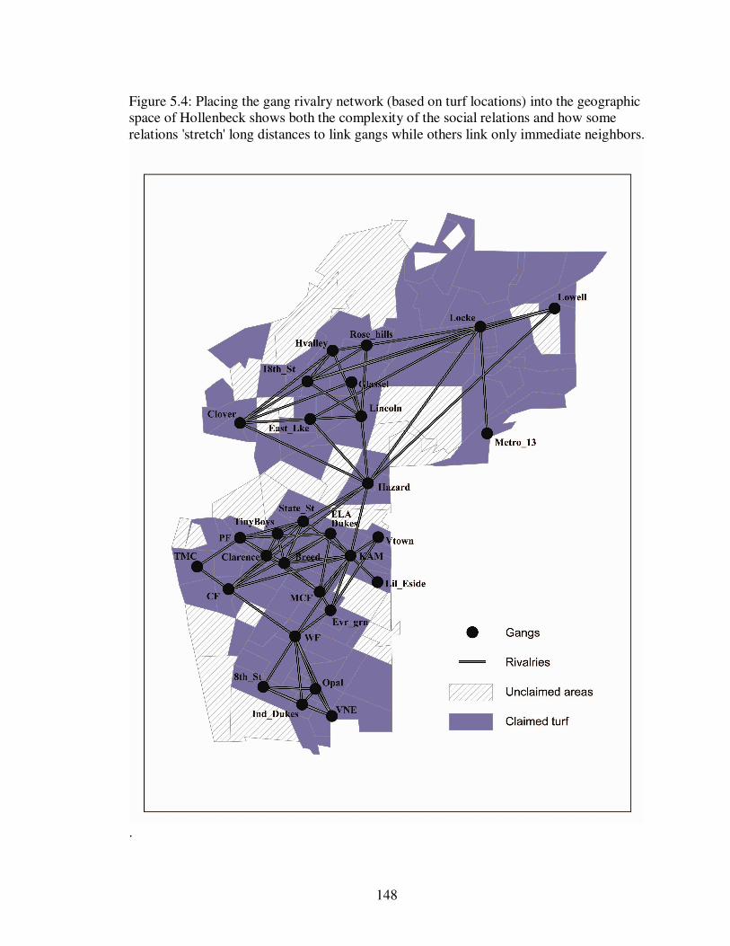
148

Figure 5.4: Placing the gang rivalry network (based on turf locations) into the geographic space of Hollenbeck shows both the complexity of the social relations and how some relations 'stretch' long distances to link gangs while others link only immediate neighbors.

.

149

Figure 5.5: A dendrogram of the CONCOR positional analysis process through three splits. Each of the 30 units (29 gangs plus one unit for unclaimed turf) in Hollenbeck is classified into distinct positions at each stage of the process

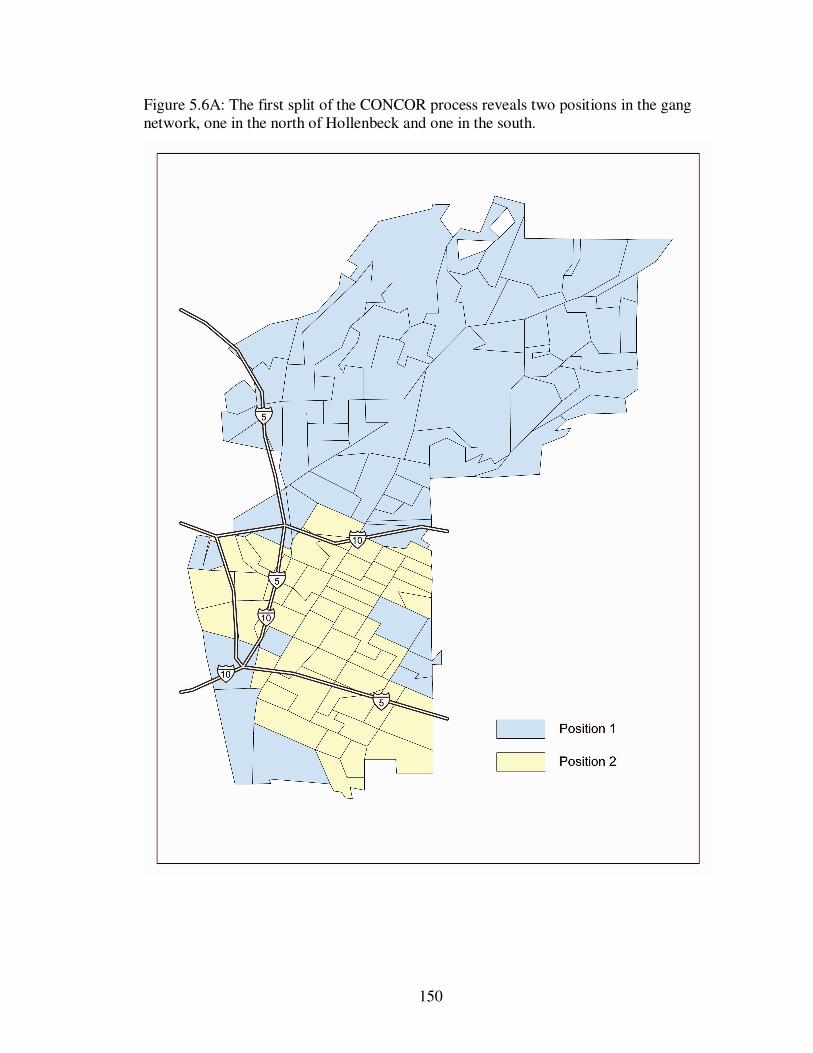
150

Figure 5.6A: The first split of the CONCOR process reveals two positions in the gang network, one in the north of Hollenbeck and one in the south.

151

Figure 5.6B: The second split of the CONCOR process subdivides each of the first two positions.

152

Figure 5.6C: The third split of the CONCOR process continues to subdivide positions. In both the north and south areas of Hollenbeck, core-periphery positions continue to be suggested.

153

CHAPTER 6

CONCLUSIONS

Quantitative spatial analyses of social behavior within criminology have

progressed significantly within the last decade, but further advances have been limited by

several factors, the most notable of which is a need for a more rigorous theoretical

approach through which we can better understand the processes of gang-related violence.

The research presented in this dissertation has attempted to contribute to this endeavor by

focusing on the geography of gang violence within a single area of a city over a relatively

short period of time. By integrating contemporary thinking in human geography about the

social production of space and place with concepts and methods in social network

analysis and spatial criminology, this study has presented an alternative framework to

consider how the processes of competition, both territorial and non-territorial, contributed

to the production of differentiated spaces of gang violence in east Los Angeles. In this

chapter, I summarize the findings presented in the empirical chapters and discuss the

importance of the framework developed for this research. I also discuss issues for future

research that are also drawn from these conclusions.

DISCUSSION

As with many other social sciences, spatial regression has become an important

way to understand and incorporate context in criminology. These models typically use

spatially lagged variables as proxies for various social phenomena thought to be

responsible for the consistent finding that spatial clustering of crime events remains even

after controlling for place-to-place variations in compositional effects such as race,

154

ethnicity and poverty. These efforts are a positive first step but this research demonstrates

that the way in which space is incorporated into such models requires careful

consideration. Specifications of the spatial weights matrix that rely on spatial contiguity

to define the spatial reach of the various social processes posited to be responsible for

clustering forces researchers to assume that all such processes decay rapidly over

geographic distance, and therefore matter only among spatially contiguous neighbors.

Furthermore, even when multiple social processes are considered, the conventional

modeling approach is to specify a single spatial weights matrix rather than specify

different kinds of connections between places for different social processes. In addition to

making it impossible to parse the impact of one process from that of another, this is an

atheoretical approach to understanding why and how space matters.

Building on these perspectives, this research has demonstrated that “space”

continues to matter as the compositional characteristics of places cannot adequately

account for the overall geographic patterns of violence. The findings presented in this

research also verify that gang rivalries are an important mechanism in the spatial

distribution of gang-related violence. However, there is also evidence that the spatial

reach of these rivalries extends well beyond simple contiguity even when considering

different units of analysis, such as those defined by gang territorial boundaries, or at the

smaller scale of census units. That is, gang rivalries play an important role in influencing

levels of violence across the study area but the geographic scope of these rivalries is not

limited to adjacent neighbors. By carefully considering the socio-spatial dimensions of

gangs in terms of their territorial claims and the rivalry networks that connect them, it is

possible to create a spatial weights matrix that explicitly captures the geographic

155

dimensions of the patterns of social influence among the gangs. The violence committed

by, and against, gang members in a socially and geographically distinct area of Los

Angeles is largely a function of a social process that spans the local geography in such a

way that violence in non-contiguous areas impacts levels of violence in a focal

neighborhood.

There are both practical and theoretical points that merit emphasis in the face of

the above findings that have obvious implications for the application of spatial analysis in

criminology. The practical point is that different specifications of the spatial weights

matrix, or W, can impact modeling results statistically. The theoretical point is that the

analyst must be prepared to engage the question of why and how space matters. This

remains the most pressing issue for analysts: to consider how the selected specification of

W relates to one’s theoretical framework about the phenomenon of interest. In the

absence of a theoretically-grounded W specification, one is invariably left with important

and often unaddressed questions about the nature of the possible interactions. As there

remains no statistical method capable of estimating the ‘best fit’ of a spatial weight

matrix to one’s data (Leenders 2002), embodying one’s theory into the specification of W

is the only sensible recourse available.

As demonstrated in this research, grounding a model of spatial interaction in a

theory of spatiality is possible. This was done by drawing on the understanding in

geography of the importance of context to human activity and that social and spatial

processes are bound up together. This is best demonstrated in the literature through the

concept of “place,” which is associated with “historical tradition, socio-cultural relations,

context, and geo-sociological effects” (O’Loughlin 2000: 133). Given the importance of

156

territory (turf) and territorial control to the gangs of Hollenbeck, the specific socio-spatial

processes were theorized as at least partly territorial in nature, which led to the

development of a ‘hybrid’ W that captured both territorial and non-territorial competitive

interactions between the gangs. In this research, spatial interaction between the gangs in a

particular place-based context was theorized and a W that matched that theory as closely

as possible was a strong predictor of the overall geography of gang-related violence.

These findings demonstrate the value of employing such an approach. It is my hope that

demonstrating an inductive approach to theorizing spatial interaction will encourage

others to do the same.

Beyond demonstrating the potential for incorporating theory in spatial analysis is

a perhaps more meaningful contribution by this research. By using the techniques and

concepts of social network analysis, this research has offered meaningful evidence that

new spatialities can emerge from complex web of social relationships in geographic and

network space. More plainly, by theorizing, tracking, and spatializing social

relationships, this research has shown that variations in the material geography of gang-

related violence were partially formed by the geography of the rivalry network but also

clearly mediated by the relative location of each gang in geographic space. This

geographic mediation of the rivalry network is more than just an argument of space as a

mechanism of integration of social processes (e.g., Goodchild et al. 2000). Furthermore,

one would be hard pressed to reach this observation through either a conventional spatial

analysis that did not consider social relations or a conventional social network analysis

that did not consider geography.

157

A further contribution is made by demonstrating that social network analytic

techniques can not just simplify complex and multidimensional socio-spatial network

structures but also reveal new kinds of spatialities that emerge from the interplay of

different networks of relationships. For example, because the rivalry relations between

gangs at times stretch over relatively long distances and bypass territorial neighbors, the

spatialities of betweenness appear to be meaningful in the neighborhoods of Hollenbeck.

The spatiality of betweenness, or the notion that being situated between other actors

either in social space (relational betweenness), geographic space (geographical

betweenness), or both, is an important element in understanding the overall geographic

patterns of gang violence and only is revealed as such by considering the interplay of

different networks.

Although the research presented in this dissertation concerns a specific kind of

violence between specific kinds of social units in a specific locality, there are general

implications for research into other contexts. While I frame these issues here in terms of

methodology, they are drawn from the overall point regarding the importance for

theoretically information spatial analyses. First, and most importantly, the patterning of

ties in the social network, or the structure of social relations, can and should be

understood geographically. Despite arguments that geographic perspectives on social

networks (especially while utilizing social network analytic methodologies) are difficult

to achieve (Leedners 2002; Bosco 2006a), this research demonstrates relatively simple

yet powerful techniques to link relational networks with geography. Second, because

many relations have a material geographic nature, positional analyses can yield insights

into how social relations may be implicated in the production of differentiated

158

spaces/places. These insights may be particularly valuable because they are arrived at in a

novel fashion. By and large, investigations into spatiality in geography are almost

exclusively qualitative affairs. In as much as the conventional approach to spatiality may

not easily penetrate other social science disciplines where quantitative methodologies

remain central, the addition of a quantitative and empirically-minded set of techniques

that engages with issues of spatiality is significant. Third and lastly, while the methods

demonstrated in this paper are capable of standing alone, they seem particularly valuable

when used in concert with other ways of knowing. As noted in the discussion of specific

findings about the spaces of gang rivalry in Hollenbeck, the analytic methods used in this

paper answer some questions while suggesting others and are not offered as an absolute

substitute for situated and ethnographic knowledge.

FUTURE RESEARCH

This research has focused on introducing a set of approaches and techniques that

can be compatible with theoretical issues in geography concerned with the patterning of

social relations. Although this dissertation has focused on a single issue (gang violence)

in a single setting (the neighborhoods of Hollenbeck), many paths for future inquiry are

open. I wish to draw attention to possibilities based on the particular limitations of this

particular study as well as to those that I feel suggest the flexibility and applicability of

social network analysis methods and techniques to other kinds and scales of research in

geography.

From the point of view of this particular study, our findings are based on a series

of operational choices (e.g., how to measure variables of interest, coding schemes, units

159

of analysis, etc.) that could be possibly improved upon. For example, the dependent

variable in the empirical chapters was a count of violent crimes committed by or against

gang members in the Hollenbeck Policing Area between May of 2000 through December

of 2002. While this violence is therefore certainly “gang related” in that it involves gang

members in some fashion, it is not entirely certain how much of the violence is “gang

motivated” in nature (e.g., protection of turf from an incursion by rival members and

suitable to model through the rivalry and turf-based territoriality networks) as opposed to

opportunistic in nature (which may have little to do with either gang rivalries or turf

claims). Further, as the dependent variable included different types of violent crimes

(aggravated assaults, simple assaults, assault with a deadly weapon, attempted homicides,

homicides, robberies, kidnappings, and firing a gun into an inhabited dwelling/vehicle),

perhaps disaggregating robberies from assault/homicides sharpen the patterns under

investigation in this study.

From the spatial analytic perspective, perhaps the most important improvement

for future research lies not in further disaggregation of the dependent variable but of the

study area itself. Based on the traditional emphasis on areally aggregated data in spatial

criminology (the ‘ecological’ tradition), this study has used census units as the basic unit

of analysis. However, given that the crime variable is already geographically

disaggregated from any areal units (see Figure 4.3), one need not adopt existing areal

units for this type of analysis. Recent efforts in different types of analytic human

geography have emphasized the precise mapping of the location of the phenomenon of

interest (e.g., O'Loughlin and Raleigh 2008) and by using GIS-based techniques to create

new uniform units of analysis by overlaying a grid on the study site. This perspective has

160

the advantage of not privileging a particular type of areal unit and dealing with some of

the issues of the MAUP problem. However, such an approach would likely preclude the

use of social data aggregated into preexisting units (such as census units) and research

using this approach remains a largely descriptive endeavor, emphasizing mapping, rates

of diffusion, and statistical summaries (e.g., O'Loughlin and Raleigh 2008). A significant

challenge for this perspective is to connect and evaluate the descriptive findings of spatial

patterns to theories behavior of interest.

Future efforts should also attempt to incorporate dynamism and change over time.

The data used in these studies was temporally pooled and as such, the analysis presents a

presumably unchanging rivalry network and associated turf map. Social relations are

inherently dynamic and, although changes occur within existing structures, today’s

rivalries may in fact be tomorrow’s alliances. The approach presented in this dissertation

does not prevent the consideration of different network structures over time and

disaggregating networks temporally (in addition to distributing them geographically)

would be a positive step toward introducing dynamism.

Further, this research was quite parsimonious in that only rivalries and relative

location in space were considered as elements of socio-spatial network position. This

limitation undoubtedly overlooks some factors in the production of gang violence and

therefore is not a perfect example of an analysis of multiple spatialities. Nonetheless,

accepting multiple networks of relations as analytic inputs is a hallmark of the techniques

presented in this dissertation and including other kinds of relationships that would better

reflect the concerns of overlapping networks (Ettlinger 2003) or multiple spatialities

(Leitner et al. 2008) is certainly possible.

161

Lastly, positional analyses, such as the type performed in this paper, are holistic

and global in that they are concerned with the structural properties of an entire network.

However, they are also but one possible approach to applying social network analysis

methods to issues of the social construction of space. For example, an ‘egocentric’

approach, which focuses on properties of the network from the perspective of different

actors situated in particular locations, might tell a great deal more about the differences

and similarities between places (social locations) while also refocusing inquiry from

networks of gangs to networks of individuals (e.g., Ettlinger 2003).

It is my hope that through the example of Hollenbeck, the issues and methods

presented in this study encourage future research into how social networks are involved

in the social production of space and how social network analysis methods may be

utilized to understand if and how the structure of social networks have implications for

material geographic outcomes. Even when considering the limitations of the example of

gang violence in the neighborhoods of Hollenbeck, it is evident that letting

geographically-informed theories of social behavior guide a spatial analysis can lead to

meaningful insights. Although the specific findings of the gang rivalry networks in

Hollenbeck are certainly dependent of the geographic and historical context of gangs in

Hollenbeck, I believe this research has emphasized the utility of the demonstrated

concepts and methods for other topics.

162

References

Agnew, J. 1987. Place and politics: The geographical mediation of state and society.

Boston: Allen & Unwin. Allen, J. 2003. Lost geographies of power. Malden, MA: Blackwell Pub. Anderson, E. 1999. Code of the street: Decency, violence, and the moral life of the inner

city. New York: W. W. Norton & Company Anselin, L. 1988. Spatial econometrics: Methods and models. Boston: Kluwer Academic

Publishers. ———. 1995. Local indicators of spatial association - LISA. Geographical Analysis

27(1): 93–115. ———. 1998. Exploratory spatial data analysis in a geocomputational environment. In P.

Longley, S. Brooks, R. McDonnell, and B. Macmillan (eds.), Geocomputation, a

primer. New York: John Wiley & Sons. ———. 1999. Interactive techniques and exploratory spatial data analysis. In P. Longley,

M. Goodchild, D. Maguire, and D. Rhind (eds.), Geographical information systems. New York: John Wiley & Sons.

———. 2002 Under the hood: Issues in the specification and interpretation of spatial

regression models. Agricultural Economics 27(3): 247–267. ———. 2006. Spatial econometrics. In T.C. Mills & K. Patterson (eds.), Palgrave

Handbook of econometrics: Volume 1, Econometric Theory, 901-941. Basingstoke: Palgrave Macmillan.

Anselin, L., R. Florax, and S. Rey. 2004. Advances in spatial econometrics:

Methodology, tools and applications. Berlin: Springer-Verlag. Anselin L., E. Griffiths, and G. Tita. 2008. Crime mapping and hot spot analysis. In R.

Wortley & L. Mazerolle (eds.), Environmental Criminology and Crime Analysis, 97–116. Willan Publishing.

Anselin, L., I. Syabri, and Y. Kho. 2006. GeoDa: An introduction to spatial data analysis.

Geographical Analysis 38: 5–22. Bailey, T., and A. Gatrell. 1995. Interactive spatial data analysis. Harlow, UK: Addison

Wesley Longman.

163

Baller, R., L. Anselin, S. Messner, G. Deane, and D. Hawkins. 2001. Structural covariates of U.S. county homicide rates: Incorporating spatial effects. Criminology 39(3): 561–590.

Bellair, P. 2000. Informal surveillance and street crime: A complex relationship.

Criminology 38: 137–167. Bivand, R. 2002. Spatial econometrics functions in R: Classes and methods. Journal of

Geographical Systems 4(4): 405–421. Blaikie, P. 1978. The theory of the spatial diffusion of innovations: A spacious cul-de-

sac. Progress in Human Geography 2: 268–295. Blau, J., and P. Blau. 1982. Cost of inequality: Metropolitan structure and violent crime.

American Sociological Review 47(1): 114–129. Block, C., and R. Block. 1993. Street gang crime in Chicago. Research in Brief. National

Institute of Justice, Washington, D.C. Blumstein, A. 1995. Youth violence, guns, and the illicit-drug industry. Journal of

Criminal Law and Criminology 86: 10–36. Blumstein, A., and D. Cork. 1996. Linking gun availability to youth gun violence. Law

and Contemporary Problems 59(1): 5–24. Blumstein, A., and R. Rosenfeld. 1998. Explaining recent trends in US homicide rates.

Journal of Criminal Law and Criminology 88: 1175–1216. Borgatti, S., and M. Everett. 1992. Notions of position in social network analysis.

Sociological Methodology 22: 1–35 Borgatti, S., M. Everett, and L. Freeman. 2005. UCINET 6 for Windows: Software for

social network analysis. Analytic Technologies, Boston. Bosco, F. 2006a. Actor-network theory, networks, and relational approaches in Human

Geography. In Approaches to Human Geography (eds.), S. Aitken and G. Valentine. London, UK: Sage Publications.

———. 2006b. The Madres de Plaza de Mayo and three decades of human rights’

activism: Embeddedness, emotions, and social movements. Annals of the Association

of American Geographers 96: 342–365. Bowers, K., and S. Johnson. 2003. Measuring the geographical displacement and

diffusion of benefit effects of crime prevention activity. Journal of Quantitative

Criminology 19: 275–301.

164

Boulding, K. 1962. Conflict and defense. New York: Harper. Braga, A. 2001. The effects of hot spots policing on crime. The Annals of the American

Academy of Political and Social Science 578: 104–125. Brantingham, P. J., and P. L. Brantingham. 1981. Environmental criminology. Beverly

Hills: Sage Publications. Breiger, R. 1974. The duality of persons and groups. Social Forces 53:181–190. Breiger, R., S. Boorman, and P. Arabie. 1975. An algorithm for clustering relational data

with applications to social network analysis and comparison with multidimensional scaling. Journal of Mathematical Psychology 12:328–383.

Bursik, R., and H. Grasmick. 1993. Neighborhoods and crime: The dimensions of

effective community control. San Francisco, Lexington Books. Burt, R. 1987. Social contagion and innovation: cohesion versus structural equivalence.

American Journal of Sociology 92: 1287-1335. ———. 1992. Structural holes: The social structure of competition. Cambridge, MA:

Harvard University Press. Cahill, M., and G. Mulligan. 2007. Using geographically weighted regression to explore

local crime patterns. Social Science Computer Review 25: 174–193. Case, A., H. Rosen, J. Hines. 1993. Budget spillovers and fiscal policy interdependence:

Evidence from the states. Journal of Public Economics 52: 285–307. Casetti, E. 1997. The expansion method, mathematical modeling, and spatial

econometrics. International Regional Science Review 20: 9–33. Cliff, A., and J. Ord. 1973. Spatial autocorrelation. London: Pion. ———. 1981. Spatial processes, models, and applications. London: Pion. Cohen, J., and G. Tita. 1999a. Editors’ introduction. Journal of Quantitative Criminology

154: 373–378. ———. 1999b. Diffusion in homicide: Exploring a general method for detecting spatial

diffusion processes. Journal of Quantitative Criminology 154: 451–493. Cohen, J., D. Cork, J. Engberg, and G. Tita. 1998. The role of drug markets and gangs in

local homicide rates. Homicide Studies 2: 241–262.

165

Cohen, L., and M. Felson. 1979. Social change and crime rate trends: A routine activities approach. American Sociological Review 44: 588–608.

Coleman, J., E. Katz, and H. Menzel. 1966. Medical innovation: A diffusion study. New

York, Bobbs-Merrill. Collinge, C. 2005. The différance between society and space: Nested scales and the

returns of spatial fetishism. Environment and Planning D: Society and Space 23(2): 189–206.

Cooley, S. 2008. Gang crime and violence in Los Angeles County: Findings and

proposals from the District Attorney's Office. Available online at http://da.co.la.ca.us/pdf/LADA_Gang_Crime_and_Violence_APR_2008.pdf last accessed 29 May 2009.

Cork, D. 1999. Examining space–time interaction in city-level homicide data: Crack

markets and the diffusion of guns among youth. Journal of Quantitative Criminology 154: 379–406.

Cox, K. 1998. Spaces of dependence, spaces of engagement and the politics of scale, or:

looking for local politics. Political Geography 17: 1–23. Cox, K., M. Low, and J. Robinson. 2008. Political geography: Traditions and turns. In K.

Cox, M. Low, and J. Robinson (eds.), The SAGE handbook of political geography, 1–14. Thousand Oaks, CA: Sage.

Cressie, N. 1993. Statistics for spatial data, rev. ed. New York: Wiley and Sons. Cresswell, T. 1996. In place/out of place: Geography, ideology and transgression.

Minneapolis: University of Minnesota Press. ———. 2004. Place: A short introduction. Malden, MA: Blackwell. Cullen, J., and S. Levitt. 1997. Crime, urban flight, and the consequences for cities.

National Bureau of Economic Research, working paper 5737. Decker, S. 1996. Collective and normative features of gang violence. Justice Quarterly

13: 243–264. Dicken, P., P. Kelly, K. Olds, and H. W.-C. Yeung. 2001. Chains and networks,

territories and scales: Towards a relational framework for analysing the global economy. Global Networks 1(2): 89–112.

Diehl, P., and G. Goertz. 2000. War and peace in international rivalry. Ann Arbor, MI:

The University of Michigan Press.

166

Doreian, P. 1980. Linear models with spatially distributed data: Spatial disturbances or spatial effects? Sociological Methods and Research 9: 29–60.

Doreian, P., and N. Hummon. 1976. Modeling social processes. New York: Elsevier. Doreian, P., V. Batageli, and A. Ferligoj. 2005. Positional analyses of sociometric data.

In Models and methods in social network analysis, (eds.) P. J. Carrington, J. Scott and S. Wasserman, 77–97. Cambridge; New York: Cambridge University Press.

Durkheim, É. 1897. Il suicidio dal punto di vista sociologico. Rivista italiana di

sociologia 1: 17–27. Eagle, M., N. Macy, and R. Claxton. 2010. Network diversity and economic

development. Science 328: 1029–1031. Elffers, H. 2003. Analyzing neighbourhood influence in criminology. Journal of the

Netherlands Society for Statistics and Operations Research 57(3): 347–367. Emirbayer, M. 1997. Manifesto for relational sociology. American Journal of Sociology

103: 281–317. Emirbayer, M., and J. Goodwin. 1994. Network analysis, culture, and the problem of

agency. American Journal of Sociology 99: 1411–1454. Entrikin, J. 1991. The betweenness of place: Toward a geography of modernity.

Baltimore: Johns Hopkins University Press. Ettlinger, N. 2003. Cultural economic geography and a relational and microspace

approach to trusts, rationalities, networks, and change in collaborative workplaces. Journal of Economic Geography 3(2): 145–171.

Ettlinger, N., and F. Bosco. 2004. Thinking through networks and their spatiality: a

critique of the US (public) war on terrorism and its geographic discourse. Antipode 36: 249–271.

Everett, M., and S. Borgatti. 2005. Extending centrality. In Models and methods in social

network analysis, (eds.) P. Carrington, J. Scott, and S. Wasserman, 57–76. New York: Cambridge University Press.

Fagan, J., F. Zimring, and J. Kim. 1998. Declining homicide in New York: a tale of two

trends. Journal of Criminal Law and Criminology 88: 1277-1324. Feld, S. 1981. The focused organization of social ties. American Journal of Sociology 86:

1015–1035.

167

Flint, C. 1998. Forming electorates, forging spaces: The Nazi Party vote and the social construction of space. American Behavioral Scientist 41(9): 1282–1303.

———. 2002. The theoretical and methodological utility of space and spatial statistics:

The Nazi Party in geographical context. Historical Methods 35(1): 32–42. Flint, C., P. Diehl, J. Scheffran, J. Vasquez, and S-H. Chi. 2009. Conceptualizing

ConflictSpace: Towards a geography of relational power and embeddedness in the analysis of interstate conflict. The Annals of the Association of American

Geographers 99(5): 827–835. Florax, R., & Rey, S. 1995. The impacts of misspecified spatial interaction in linear

regression models. In L. Anselin and R. Florax (eds.), New directions in spatial

econometrics, 111–135. Berlin: Springer. Fotheringham, A. 1989. Scale-independent spatial analysis. In M. Goodchild, and S.

Gopal (eds.), Accuracy of spatial databases, 221–228. London: Taylor and Francis. ———. 1997. Trends in quantitative methods I: Stressing the local. Progress in Human

Geography 21: 88–96. Fotheringham, A., M. Charlton, and S. Brundson. 2002. Geographically weighted

regression: The analysis of spatially varying relationships. New York: John Wiley. Fotheringham, A., and P. Rogerson. 1993. GIS and spatial analytical problems.

International Journal of Geographic Information Systems 7: 3–19. Fotheringham, A., and D. Wong. 1991. The modifiable areal unit problem in statistical

analysis. Environment and Planning A 23: 1025–1044. Freeman, L. 1977. A set of measures of centrality based on betweenness. Sociometry

40(1): 35–41 ———. 1979. Centrality in social networks: Conceptual clarification. Social Networks

1(3): 215–239. ———. 2005. Graphic techniques for exploring social network data. In P. Carrington, J.

Scott and S. Wasserman (eds.), Models and methods in social network analysis, 248–269. Cambridge; New York: Cambridge University Press.

Friedkin, N. 1984. Structural cohesion and equivalence explanations of social

homogeneity. Sociological Methods and Research 12(3): 235–261. ———. 1991. Theoretical foundations for centrality measures. American Journal of

Sociology 96(6): 1478–1504.

168

Galaskiewicz, J., and R. Burt. 1991. Interorganizational contagion in corporate philanthropy. Administrative Science Quarterly 36: 88–105.

Gehlke, C., and K. Biehl. 1934. Certain effects of grouping upon the size of the

correlation coefficient in census tract material. Journal of the American Statistical

Association 29: 169–170. Getis, A. 2009. Spatial weight matrices. Geographical Analysis 41: 404–410. Getis, A., and J. Aldstadt. 2004. Constructing the spatial weights matrix using a local

statistic. Geographical Analysis 36: 90–104. Getis, A., and J. Ord. 1992. The analysis of spatial association by use of distance

statistics. Geographical Analysis 24: 189–206. Goodchild, M. 2004. GIScience, geography, form, and process. Annals of the Association

of American Geographers 944: 709–714. Goodchild, M., L. Anselin, R. Appelbaum, and B. Harthorn. 2000. Toward spatially

integrated social science. International Regional Science Review 23: 139–159. Gorman, D., P. Speer, P. Gruenewald, and E. Labouvie. 2001. Spatial dynamics of

alcohol availability, neighborhood structure and violent crime. Journal of Studies on

Alcohol 625: 628–636. Gould, R. 1991. Multiple networks and mobilization in the Paris Commune, 1870.

American Sociological Review 56: 716–729. Grabher, G. 2008. Trading routes, bypasses, and risky intersections: Mapping the travels

of ‘networks’ between economic sociology and economic geography. Progress in

Human Geography 30 (2): 163–189. Graif, C. and Sampson, R. 2009. Spatial heterogeneity in the effects of immigration and

diversity on neighborhood homicide rates. Homicide Studies 13: 242–260. Grannis, R. 2009. From the ground up: Translating geography into community through

neighbor networks. Princeton, NJ: Princeton University Press. Granovetter, M. 1973. The strength of weak ties. American Journal of Sociology 78(6):

1360–1381. ———. 1985. Economic action and economic structure: the problem of embeddedness.

American Journal of Sociology 91(3): 481–510.

169

———. 1992. Problems of explanation in economic sociology. In R. G. Eccles and N. Nohria (eds.), Networks and organizations: Structure, form, and action, 25–26. Boston: Harvard Business School Press.

Grattet, R., V. Jenness, and T. Curry. 1998. The homogenization and differentiation of

‘hate crime’ law in the U.S., 1978-1995: An analysis of innovation and diffusion in the criminalization of bigotry. American Sociological Review 63: 286–307.

Greenbaum, R. 2002. A spatial study of teachers' salaries in Pennsylvania school

districts. Journal of Labor Research 23: 69–86. Griffith, D. 1983. The boundary value problem in spatial statistical analysis. Journal of

Regional Science 23: 377–378. ———. 1987. Spatial autocorrelation: a primer. Washington, D.C.: Association of

American Geographers. ———. 1996. Some guidelines for specifying the geographic weights matrix contained

in the spatial statistical models. In S. Arlinghaus (ed.), Practical handbook of spatial

statistics, 65–82. Boca Raton: CRC Press. Griffiths, E., and J. Chavez. 2004. Communities, street guns, and homicide trajectories in

Chicago, 1980-1995: Merging methods for examining homicide trends across space and time. Criminology 424: 941–978.

Groff, E., T. McEwen. 2006. Exploring the spatial configuration of places related to

homicide events. Final Report. National Institute of Justice. Washington, DC Groff, E., D. Weisburd, and N. Morris 2009. Where the action is at places: Examining

spatio-temporal patterns of juvenile crime at places using trajectory analysis and GIS. In D. Weisburd, W. Bernasco, and G. Bruinsma (eds.), Putting crime in its place 61–86. New York: Springer.

Haining, R. 1990. Spatial data analysis in the social and environmental sciences.

Cambridge: Cambridge University Press. ———. 2003. Spatial data analysis: Theory and practice. Cambridge: Cambridge

University Press. ———. 2009. The special nature of spatial data. In S. Fotheringham and P. Rogerson

(eds.), The SAGE Handbook of spatial analysis. Thousand Oaks, CA: Sage. Herbert, S. 1997. Policing space: territoriality and the Los Angeles Police Department.

Minneapolis: University of Minnesota Press.

170

Herod A., and M. Wright. 2002. Placing scale: an introduction. In A. Herod and M. Wright (eds.), Geographies of power: placing scale, 1–14. Oxford: Blackwell.

Hess, M. 2004. ‘Spatial’ relationships? Towards a reconceptualization of embeddedness.

Progress in Human Geography 28(2): 165–186. Hipp, J. 2007. Block, tract, and levels of aggregation: Neighborhood structure and crime

and disorder as a case in point. American Sociological Review 72: 659–680. ———. 2010. Micro-structure in micro-neighborhoods: A new social distance measure,

and its effect on individual and aggregated perceptions of crime and disorder. Social

Networks 32: 148–159. Hipp, J., G. Tita, and L. Boggess. 2009. Inter- and intra-group interactions: The case of

everyday violent crime as an expression of group conflict or social disorganization. Criminology 47(2): 521–564.

Hipp, J., G. Tita, and R. Greenbaum. 2009. Drive-bys and trade-ups: examining the

directionality of the crime and residential instability relationship. Social Forces 87: 1777–1812.

Isard, W. 1956. Location and the space economy. New York, Wiley. Kahler, M. 2006. Territoriality and conflict in an era of globalization. In M. Kahler, (ed.),

Territoriality and conflict in an era of globalization, 1–24. Cambridge, UK: Cambride University Press.

Kellerman, A. 1996. Understanding and preventing violence: a public health perspective.

National Institute of Justice Review. Washington, D.C.: U.S. Government Printing Office.

Kennedy, D., and A. Braga. 1998. Homicide in Minneapolis: research for problem

solving. Homicide Studies 2: 263–290. Kennedy, D., A. Braga, and A. Piehl. 1997. The (un)known universe: mapping gangs and

gang violence in Boston. In D. Weisburd and T. McEwen (eds.), Crime mapping and

crime prevention, 219–262. Monsey, NY, Criminal Justice Press. Klein, M. 1971. Street gangs and street workers. Englewood Cliffs, NJ: Prentice-Hall. ———. 1995. The American street gang: Its nature, prevalence and control. New York:

Oxford University Press. Klein, M., C. Maxson, and L. Cunningham. 1991. Crack, street gangs, and violence.

Criminology 29: 623–650.

171

Krivo, L. and R. Peterson. 1996. Extremely disadvantaged neighborhoods and urban crime. Social Forces 75: 619–650.

Kubrin, C., and R. Weitzer. 2003. Retaliatory homicide: Concentrated disadvantage and

neighborhood culture. Social Problems 50: 157–180. Kubrin, C., and E. Stewart. 2006. Predicting who reoffends: The neglected role of

neighborhood context in recidivism studies. Criminology 44: 165–197. Kuus, M., and J. Agnew. 2008. Theorizing the state geographically: Sovereignty,

subjectivity, territoriality. In K. Cox, M. Low and J. Robinson (eds.), The SAGE

Handbook of Political Geography, 95–106. Thousand Oaks, CA: Sage. Kwan, M.-P. 2007. Mobile communications, social networks, and urban travel: Hypertext

as a new metaphor for conceptualizing spatial interaction. The Professional

Geographer 59(4): 434–446. Land, K., and G. Deane. 1992. On the large-sample estimation of regression models with

spatial or network effects terms: A two-stage least-squares approach. In P. Marsden (ed.), Sociological methodology 1992, 221–248. Oxford: Basil Blackwell.

Land, K., P. McCall, and L. Cohen. 1990. Structural covariates of homicide rates: Are

there any invariances across time and social space? American Journal of Sociology 95: 922–963.

Lantham, A. 2002. Retheorizing the scale of globalization: Topologies, actor-networks,

and cosmopolitanism. In A. Herod and M. Wright (eds.), Geographies of power:

Placing scale, 115–144. Oxford, UK: Blackwell. Leenders, R. 2002. Modeling social influence through network autocorrelation:

Constructing the weight matrix. Social Networks 24: 21–47. Lefebvre, H. 1991. The production of space, trans. D. Nicholson-Smith. Oxford: Basil

Blackwell. Leitner, H., E. Sheppard, and K. Sziarto. 2008. The spatialities of contentious politics.

Transactions of the Institute of British Geographers 33(2): 157–172. Loftin, C. 1986. Assultive violence as a contagious process. Bulletin of New York

Academy of Medicine 62: 550-555. Lorrain, F. and H. White. 1971. Structural equivalence of individuals in social networks.

Journal of Mathematical Sociology 1: 49–80. Los Angeles Police Department. 2008. Hollenbeck Crime Statistics. Available online at

http://www.lapdonline.org/assets/pdf/hbkprof.pdf (last accessed 29 May 2009).

172

Mamadouh, V., O. Kramsch, and M. Van der Velde. 2004. Articulating local and global

scales. Tijdschrift voor Economische en Sociale Geografie 95: 455–466. Marsden, P., and N. Friedkin. 1993. Network studies of social influence. Sociological

Methods & Research 22: 125–149. Marston, S., J. Jones, and K. Woodward. 2005. Human geography without scale.

Transactions of The Institute of British Geographers 30: 416–432. Massey, D. 1993. Power-geometry and a progressive sense of place. In J. Bird, B. Curtis,

T. Putnam, G. Robertson, and L. Tickner (eds.), Mapping the future: Local cultures,

global change, 59–69. London: Routledge. ———. 1997. A global sense of place. In T. Barnes and D. Gregory (eds.), Reading

Human Geography, 315–323. London: Arnold. ———. 1999. Power geometries and the politics of timespace. Heidelberg: Heidelberg

University Press. McGloin, J. 2005. Policy and intervention considerations of a network analysis of street

gangs. Criminology and Public Policy 4: 607–636. McPherson, M., L. Smith-Lovin and J. Cook. 2001. Birds of a feather: Homophily in

social networks. Annual Review of Sociology 27: 415–444. McMaster, R, and E. Sheppard, E. 2004. Introduction: scale and geographic inquiry. In E.

Sheppard and R. McMaster (eds.), Scale and geographic inquiry, 1–22. Oxford: Blackwell.

Mears, D., and A. Bhati. 2006. No community is an island: The effects of resource

deprivation on urban violence in spatially and socially proximate communities. Criminology 44(3): 509–548.

Messner, S., and L. Anselin. 2004. Spatial analyses of homicide with areal data. In M.

Goodchild & D. Janelle (eds.), Spatially integrated social science, 127–144. Oxford: Oxford University Press.

Messner, S., L. Anselin, R. Baller, D. Hawkins, G. Deane, and S. Tolnay. 1999. The

spatial patterning of county homicide rates: An application of exploratory spatial Data analysis. Journal of Quantitative Criminology 15(4): 423–450.

Messner, S., and K. Tardiff. 1986. The social ecology of urban homicide: An application

of the ‘routine activities’ approach. Criminology 22: 241–267.

173

Moore, J. 1985. Isolation and stigmatization in the development of an underclass: The case of Chicano gangs in East Los Angeles. Social Problems 33: 1–12.

———. 1991. Going down to the barrio: Homeboys and homegirls in Change.

Philadelphia: Temple University Press. Morenoff, J. 2003. Neighborhood mechanisms and the spatial dynamics of birth weight.

American Journal of Sociology 108: 976–1017. Morenoff, J., and R. Sampson. 1997. Violent crime and the spatial dynamics of

neighborhood transition: Chicago, 1970–1990. Social Forces 76(1): 31–64. ———. 2004. Spatial (dis)advantage and homicide in Chicago neighborhoods. In M.

Goodchild and D. Janelle (eds.), Spatially integrated social science, 145–170. New York: Oxford Press.

Morenoff, J., R. Sampson, and S. Raudenbush. 2001. Neighborhood inequality, collective

efficacy, and the spatial dynamics of urban violence. Criminology 39: 517–560. Murdoch, J., and T. Marsden. 1995. The spatialization of politics: Local and national

actor-spaces in environmental conflict. Transactions of the Institute of British

Geographers 20(3): 368–380. Murphy, K., and R. Topel. 1985. Estimation and inference in two-step econometric

models. Journal of Business and Economic Statistics 3: 370–379. Newman, D. 2006. The resilience of territorial conflict in an era of globalization. In M.

Kahler (ed.), Territoriality and conflict in an era of globalization, 85–110. Cambridge, UK: Cambride University Press.

O'Loughlin, J. 2000. Geography as space and geography as place: The divide between

political science and political geography continues. Geopolitics 5: 126–137. ———. 2003. Spatial analysis in political geography. In J. Agnew, K. Mitchell and G. Ó

Tuathail (eds.), A companion to Political Geography, 30–46. Malden, MA: Blackwell Pub.

O'Loughlin, J., and C. Raleigh. 2008. Spatial analysis of civil war violence. In K. Cox,

M. Low, and J. Robinson (eds.), The SAGE Handbook of Political Geography, 493–508. Thousand Oaks, CA: Sage.

Openshaw, S. 1984. The modifiable areal unit problem. Concepts and techniques in

modern Geography 38. Norwich, CT: Geobooks.

174

———. 1996. Developing GIS-relevant zone-based spatial analysis methods. In: P. Longley and M. Batty (eds.), Spatial analysis: Modeling in a GIS environment, 55 –73. New York: Wiley.

Openshaw, S., and P. Taylor. 1979. A million or so correlation coefficients: Three

experiments on the modifiable areal unit problem. In N. Wrigley (ed.), Statistical

applications in the spatial sciences, 127–144. London: Pion. ———. 1981. The modifiable areal unit problem. In N. Wrigley and R. Bennett (eds.),

Quantitative geography: A British view, 60–69. London: Routledge and Kegan Paul. Ord, J. 1975. Estimation methods for models of spatial interaction. Journal of the

American Statistical Association 70: 120–126. Ord, J., and A. Getis. 1995. Local spatial autocorrelation statistics: Distributional issues

and an application. Geographical Analysis 27: 286–306. Paasi, A. 2003. Territory. In J. Agnew, K. Mitchell and G. Ó Tuathail (eds.), A

companion to political geography, 109–122. Malden, MA: Blackwell Pub. Pred, A. 1984. Place as historically contingent process: Structuration and the time-

geography of becoming places. Annals of the Association of American Geographers 74: 279–297.

Radil, S., C. Flint, and G. Tita. 2010. Spatializing social networks: Using social network

analysis to investigate geographies of gang rivalry, territoriality, and violence in Los Angeles. Annals of the Association of American Geographers 100(2): 307–326.

Reiss, A., and D. Farrington. 1991. Advancing knowledge about co-offending: Results

from a prospective longitudinal survey of London males. Journal of Criminal Law

and Criminology 82: 360–395. Relph, E. 1976. Place and placelessness. London: Pion. Robinson, W. 1950. Ecological correlation and the behavior of individuals. American

Sociological Review 15: 351–357. Rogers, E. 1983. Diffusion of innovations. New York: Free Press. Rosenfeld, R., T. Bray, and A. Egley. 1999. Facilitating violence: A comparison of gang-

motivated, gang-affiliated, and nongang youth homicides. Journal of Quantitative

Criminology 15(4): 494–516. Ross, C. 2000. Neighborhood disadvantage and adult depression. Journal of Health and

Social Behavior 41: 177–187.

175

Rushton, G., R. Krishnamurthy, D. Krishnamurti, P. Lolonis, and H. Song. 1996. The spatial relationship between infant mortality and birth defect rates in a U.S. city. Statistics in Medicine 15: 1907–1909.

Sack, R. 1986. Human territoriality: Its theory and history. Cambridge, UK: Cambridge

University Press. Sack, R. 1997. Homo Geographicus: A framework for action, awareness, and moral

concern. Baltimore, MD: Johns Hopkins University Press. Sampson, R. 1986. Crime in cities: Formal and informal social control. In A. Reiss and T.

Michael (eds.), Communities and crime, 271–311. Chicago: University of Chicago Press.

——— 1988 Local friendship ties and community attachment in mass society: A multi

level systemic model. American Journal of Sociology 53: 766–779. ———. 2004. Networks and neighbourhoods: The implications of connectivity for

thinking about crime in the modern city. In H. McCarthy, P. Miller, and P. Skidmore (eds.), Network logic: who governs in an interconnected world? 157–166. London, Demos.

———. 2008. “After school” Chicago: Space and the city. Urban Geography 292: 127–

137. Sampson, R., and W. Groves. 1989. Community structure and crime: Testing social-

disorganization theory. American Journal of Sociology 94: 774–802. Sampson, R., and P. Sharkey. 2008. Neighborhood selection and the social reproduction

of concentrated racial inequality. Demography 451: 1–29. Sampson, R., J. Morenoff, and T. Gannon-Rowley. 2002. Assessing neighborhood

effects: Social processes and new directions in research. Annual Review of Sociology 28: 443–478.

Sampson, R., S. Raudenbush, and F. Earls. 1997. Neighborhoods and violent crime: A

multilevel study of collective efficacy. Science 277: 918–924. Shaw, C., and H. McKay. 1942. Juvenile delinquency and urban areas. Chicago:

University of Chicago Press. Sheppard, E. 2002. The spaces and times of globalization: Place, scale, networks, and

positionality. Economic Geography 78(3): 307–330. Simmel, G. 1955. Conflict and the web of group affiliations. New York: Free Press.

176

Smith, N. 1992. Contours of a spatialized politics: homeless vehicles and the production of geographical space. Social Text 33: 54–81.

Smith, W., S. Frazee, and E. Davison. 2000. Furthering the integration of routine Activity

and social disorganization theories: Small units of analysis and the study of street robbery as a diffusion process. Criminology 38: 489–523.

Snyder, D. and E. Kick. 1979. Structural position in the world system and economic

growth, 1955–1970: A multiple-network analysis of transnational interactions. The

American Journal of Sociology 84(5): 1096–1126. Staeheli, L. 2003. Place. In J. Agnew, K. Mitchell and G. Ó Tuathail (eds.), A companion

to political geography, 158–170. Malden, MA: Blackwell Pub. StataCorp. 2005. Statistical software: Release 8.0. Stata Corporation, College Station,

TX. Swyngedouw, E. 2004. Scaled geographies: nature, place and the politics of scale. In E.

Sheppard, and R. McMaster (eds.), Scale and geographic inquiry, 129–153. Oxford: Blackwell.

Taniguchi, T., J. Ratcliffe, and R. Taylor. 2011. Gang set space, drug markets, and crime:

violent and property crimes around drug corners in Camden, Journal of Research in Crime and Delinquency.

Taylor, P. 1982. A materialist framework for political geography. Transactions of the

Institute of British Geographers 7: 15–34. Taylor, R., S. Gottfredson, and S. Brower. 1984. Block crime and fear: Defensible space,

local social ties, and territorial functioning. Journal of Research on Crime and

Delinquency 21: 303–331. Thornberry, T., M. Krohn, A. Lizotte, C. Smith, and K. Tobin. 2003. Gangs and

delinquency in developmental perspective. Cambridge, UK: Cambridge University Press.

Tita, G. 2006. Neighborhoods as nodes: Combining social network analysis with spatial analysis to explore the spatial distribution of gang violence. In Workshop on Space,

Networks, and Social Influence. University of California, Irvine. Tita, G., and A. Boessen. forthcoming. Social networks and the ecology of crime: Using

social network data to understand the spatial distribution of crime. In D. Gadd, S. Karstedt, and S. Messner (eds.), The SAGE Handbook of Criminological research

methods. Thousand Oaks, CA: Sage.

177

Tita, G., and J. Cohen. 2004. Measuring spatial diffusion of shots fired activity across city neighborhoods. In M. Goodchild and D. Janelle (eds.), Spatially integrated social

science, 171–204. Oxford, UK: Oxford University Press. Tita, G., and Greenbaum, R. 2009. Crime, Neighborhoods and Units of Analysis: Putting

Space in its Place. In D. Weisburd, W. Bernasco, and G. Bruinsma (eds.), Putting

crime in its place: Units of analysis in spatial crime research, 145–170. New York: Springer.

Tita, G., and S. Radil, 2010a. Making space for theory: The challenges of theorizing

space and place for spatial analysis in criminology. Journal of Quantitative

Criminology 264: 467–479. ———. 2010b. Spatial regression models in Criminology: Modeling social processes in

the spatial weights matrix. In A. Piquero and D. Weisburd (eds.), Handbook of

quantitative Criminology, 101–121. New York: Springer. ———. 2011. Spatializing the social networks of gangs to explore patterns of violence.

Journal of Quantitative Criminology forthcoming. Tita, G., and G. Ridgeway. 2007. The impact of gang formation on local patterns of

crime. Journal of Research on Crime and Delinquency 44: 208–237. Tita, G., Cohen, J., and Engberg, J. 2005. An ecological study of the location of gang 'set

space'. Social Problems, 52, 272–299. Tita, G., K. Riley, and P. Greenwood. 2002. From Boston to Boyle Heights: The process

and prospects of a ‘pulling levers’ strategy in a Los Angeles barrio. In S. Decker (ed.), Gangs, youth violence and community policing, 102–130. Belmont, MA: Wadsworth Press.

Tita, G., K. Riley, G. Ridgeway, C. Grammich, A. Abrahamse, and P. Greenwood. 2003.

Reducing gun violence: results from an intervention in East Los Angeles. Santa Monica, CA: Rand.

Tobler, W. 1970. A computer movie simulating urban growth in the Detroit region.

Economic Geography 462: 234–240. ———. 1989. Frame independent spatial analysis. In M. Goodchild and S. Gopal (eds.),

Accuracy of spatial databases, 115–122. London: Taylor and Francis. Tuan, Y-F. 1977. Space and place: The perspective of experience. University of

Minnesota Press, Minneapolis.

178

Veysey, B., and S. Messner. 1999. Further testing of social disorganization theory: An elaboration of Sampson and Groves’ ‘Community structure and crime.’ Journal of

Research in Crime and Delinquency 36: 147–156. Vigil J. 1988. Barrio gangs: Street life and identity in Southern California. Austin, TX:

University of Texas Press. ———. 2002. A rainbow of gangs: Street cultures in the mega-city. Austin, TX:

University of Texas Press. Ward, M., and K. Gleditsch. 2008. Spatial regression models. Thousand Oaks, CA: Sage. Wasserman, S., and K. Faust. 1994. Social network analysis: Methods and applications.

Cambridge, UK: Cambridge University Press. Wellman, B. 1988. Structural analysis: From methods and metaphor to theory and

substance. In B. Wellman and S. Berkowitz (eds.), Social structures: A network

approach, 19–61. New York: Cambridge University Press. Weisburd, D., W. Bernasco, and G. Bruinsma (eds.). 2009. Putting crime in its place:

Units of analysis in spatial crime research. New York: Springer. Weisburd, D., L. Wyckoff, J. Ready, J. Eck, J. Hinkle, and F. Gajewski. 2006. Does

crime just move around the corner?: A controlled study of spatial displacement and diffusion of crime control benefits in two crime hotspots. Criminology 44: 549–592.

Whyte, W. 1943. Street corner society. Chicago: University of Chicago Press. Wilkinson, D., and J. Fagan. 1996. Understanding the role of firearms in violence scripts:

The dynamics of gun events among adolescent males. Law and Contemporary

Problems 59: 55–90. Wolpert, J. 1964. The decision process in spatial context. Annals of the Association of

American Geographers 54(4): 337–358.