spatio-temporal analysis of water quality parameters in
TRANSCRIPT

water
Article
Spatio-Temporal Analysis of Water QualityParameters in Machángara River with NonuniformInterpolation Methods
Iván P. Vizcaíno 1,*, Enrique V. Carrera 1, Margarita Sanromán-Junquera 2,Sergio Muñoz-Romero 2, José Luis Rojo-Álvarez 2 and Luis H. Cumbal 3
1 Departamento de Eléctrica y Electrónica, Universidad de las Fuerzas Armadas ESPE,Av. General Rumiñahui s/n, P.O. Box 171-5-231B, Sangolquí, Ecuador; [email protected]
2 Department of Signal Theory and Communications and Telematic Systems and Computation,Universidad Rey Juan Carlos, Camino del Molino S/N, 28942 Fuenlabrada, Madrid, Spain;[email protected] (M.S.-J.); [email protected] (S.M.-R.); [email protected] (J.L.R.-Á.)
3 Centro de Nanociencia y Nanotecnología, Universidad de las Fuerzas Armadas ESPE,Av. General Rumiñahui s/n, P.O. Box 171-5-231B, Sangolquí, Ecuador; [email protected]
* Correspondence: [email protected]; Tel.: +593-2398-9400 (ext. 1873)
Academic Editor: Richard SkeffingtonReceived: 25 July 2016; Accepted: 28 October 2016; Published: 4 November 2016
Abstract: Water quality measurements in rivers are usually performed at intervals of days or monthsin monitoring campaigns, but little attention has been paid to the spatial and temporal dynamics ofthose measurements. In this work, we propose scrutinizing the scope and limitations of state-of-the-artinterpolation methods aiming to estimate the spatio-temporal dynamics (in terms of trends andstructures) of relevant variables for water quality analysis usually taken in rivers. We used a databasewith several water quality measurements from the Machángara River between 2002 and 2007 providedby the Metropolitan Water Company of Quito, Ecuador. This database included flow rate, temperature,dissolved oxygen, and chemical oxygen demand, among other variables. For visualization purposes,the absence of measurements at intermediate points in an irregular spatio-temporal sampling grid wasfixed by using deterministic and stochastic interpolation methods, namely, Delaunay and k-NearestNeighbors (kNN). For data-driven model diagnosis, a study on model residuals was performedcomparing the quality of both kinds of approaches. For most variables, a value of k = 15 yieldeda reasonable fitting when Mahalanobis distance was used, and water quality variables were betterestimated when using the kNN method. The use of kNN provided the best estimation capabilities inthe presence of atypical samples in the spatio-temporal dynamics in terms of leave-one-out absoluteerror, and it was better for variables with slow-changing dynamics, though its performance degradedfor variables with fast-changing dynamics. The proposed spatio-temporal analysis of water qualitymeasurements provides relevant and useful information, hence complementing and extending theclassical statistical analysis in this field, and our results encourage the search for new methodsovercoming the limitations of the analyzed traditional interpolators.
Keywords: water quality; interpolation; smoothing; Delaunay; kNN
1. Introduction
Pollution is related to the introduction into the environment of substances, from anthropogenicor natural origin, which are harmful or toxic to humans and ecosystems. Pollution usually alters thechemical, physical, biological, or radiological integrity of soil, water, and living species, resultingin alterations of the food chain, with effects on human health [1,2]. In particular, water pollution ismainly due to the increment in urban and industrial density. Growing population waste poses a threat
Water 2016, 8, 507; doi:10.3390/w8110507 www.mdpi.com/journal/water

Water 2016, 8, 507 2 of 17
to public health and jeopardizes the continuous use of water reserves [3]. For example, contaminationof watercourses is a consequence of wastewater discharge, from municipal, industrial, or farmingrunoffs [4]. Typically, urban wastewater is a complex mixture containing water (usually over 99%)mixed with organic and inorganic compounds, both in suspension and dissolved with very smallconcentrations (mg/L) [5]. Globally, two million tons of wastewater are discharged into the worldwaterways [6]. Wastewater Treatment Plants (WWTPs) are used to combat water pollution of rivers incommunities (municipalities) reducing suspended solids and the organic load to accelerate the naturalprocess of water purification [3,7].
On the other hand, several properties and factors are usually considered in the water qualityanalysis and in the monitoring of pollution water sources in order to assess the impact of water pollutionon flora, fauna, and humans. Water appearance, color or turbidity, temperature, taste, and smell oftendescribe the physical properties of drinking water, whereas the water chemical characterization includesthe analysis of organic and inorganic substance concentrations. Microbiological features are related topathogenic agents (bacteria, viruses, and protozoa), which are relevant to public health and usuallymodify the water chemistry. In addition, radiological factors could be also considered in areas wherewater comes into contact with radioactive substances [8]. Other specifications such as water hardness,pH, acidity, oils, and fats can also be taken into account in the water quality analysis.
Water quality monitoring focuses on programmed sampling, measurement, and recording ofregulated water quality parameters. The water quality management in rivers can be more efficientwhen: (1) monitoring of rivers is continuous, hence its seasonal behavior can be characterized; (2) thesampling period is based on the spatio-temporal dynamics (trends or patterns) of the measuredvariables; (3) the choice of the sampling sites takes into account the basin irregularities; and(4) other factors at the study area are taken into consideration, such as population and industrialgrowth. Measurements are not usually taken uniformly at determined locations and times during themonitoring campaigns, and the pollutant concentrations in river waters do not follow linear variations.Therefore, the use of mathematical models with basic physics (that govern the transport process ofpollution) and linear models can be complemented with data-driven models for modeling the rivercontaminants dynamics, in the sense of trends and spatio-temporal structures [9].
For these reasons, several scientific works have scrutinized different spatio-temporal analysisof water quality from a statistical point of view, in order to understand their behavior and help togenerate water decontamination designs in a more efficient way. Siyue et al. analyzed up to 41 sites atthe Han River (China) during 2005 and 2006 in order to explore the spatio-temporal variations in thebasin [10]. Cluster methods and analysis of variance (ANOVA) grouped the 41 sampling sites intofive statistically significant clusters. Results showed that dissolved inorganic nitrogen and nitrates hadlarge spatial variability, while nitrogen had a relatively higher concentration in wet seasons comparedwith dry seasons, and phosphorous had the opposite trend. On the other hand, Serre et al. usedthe Bayesian maximum entropy to analyze spatio-temporal variability of water quality parametersin the case of phosphate estimation along the Raritan River basin (New Jersey, USA) between 1990and 2002 [11]. The database consisted of 1305 phosphate measurements at 55 monitoring stations.Their results showed that the spatio-temporal analysis improves the purely spatial analysis when thewater samples are noisy and scarce. In addition, Duan et al. proposed a statistical multivariate analysisincluding cluster analysis, discriminant analysis and principal component analysis/factor analysis todistinguish spatio-temporal variation of water quality and contaminants [12]. Fourteen parameterswere studied in 28 sites of Eastern Poyang Lake Basin, Jiangxi Province of China from January 2012 toApril 2015. This work also pointed out the spatio-temporal analysis as a tool to help in the optimizationof the water quality monitoring programs. The impact of wastewater was also scrutinized in a detailedanthropogenic study of the Henares River (Spain) [13]. The Henares River runs through residential,industrial, and farming areas. Thus, strategic points were chosen along the river, with five stationsupstream of a WWTP, and five stations downstream. Six monitoring campaigns were carried outbetween April and June 2010, assembling 36 water samples altogether. Descriptive statistics, such as
Water 2016, 8, 507 3 of 17
frequency or mean of pollutant concentration and uni-dimensional graphical representations were usedto analyze their spatial and temporal evolution, showing the influence of the wastewater discharge andof the farm areas’ proximity. For example, high concentrations of polycyclic aromatic hydrocarbons,which are usually adsorbed on the river sediments, still continued along the Henares River regardlessof season. Note that all these results point out the relevance of the observable dynamics of thesepollutants with respect to time and space. This work pointed out the importance of the spatio-temporalanalysis in order to visualize the trends of some compounds in the rivers, which could determinea possible relationship between river water contamination and wastewater effluent discharges.
However, and to the best of our knowledge, the variability of measurements jointly expressed inspace and time has not been explored for analyzing the spatio-temporal distributions of water qualityvariables. In the present work, we propose scrutinizing the scope and limitations of state-of-the-artinterpolation methods aiming to estimate the spatio-temporal dynamics (in terms of trends andstructures) of relevant variables for water quality analysis usually taken in rivers. For visualizationpurposes, the absence of measurements at intermediate points in an irregular spatio-temporal samplinggrid is fixed by using deterministic and stochastic interpolation methods, namely, Delaunay andk-Nearest Neighbors (kNN). For data-driven model diagnosis, a study on model residuals is performed,allowing for comparison of the model quality for both kinds of approaches.
These methods are here applied to pollution measurements at the Machángara River and itstributaries in Quito, Ecuador. Whereas several previous studies of Machángara River pollution havebeen made since 1977 [14], they have conducted statistical analysis on specific variables such asphosphates, pesticides, nitrates, and hydrocarbons, but a more detailed and complete view of thewastewater dynamics can still be addressed.
The rest of this paper is as follows. In Section 2, the materials and methods are explained,including the mathematical description of the interpolation algorithms and details of the databaseused for this analysis. In Section 3, results are presented for a number of measured variables, thealgorithmic performance is benchmarked, a comparative analysis is made on the data-driven residualsof the models with both methods, and the analysis on several environmental variables and theirspatio-temporal dynamics is described. In Section 4, the results are discussed, and in Section 5,the main conclusions are presented.
2. Materials and Methods
2.1. Study Area
Quito, the capital of Ecuador, is located at approximately 2815 m above sea level, at UTMWGS84coordinates with latitude 9973588.50 [00°13′47′′ S] and longitude 776529.41 [78°31′30′′ W], as depictedin Figure 1, and it had an average temperature of 14 °C between 2002 and 2007. The MachángaraRiver was chosen for this study because it is the main wastewater collector of Quito. This river runsthrough the city from south to north, collecting wastewater at a distance of approximately 22 km, andit receives about 75% of the city waste. Along the river pathway, 25 water quality monitoring stationsare installed [14,15]. For our work, six stations were chosen in the upstream section of the River, withina reach of about 10 km, in order to monitor large amounts of wastewater. The identification of themonitoring stations is shown in Table 1, and the water quality parameters to be analyzed are describedin Table 2.
Sixty-four monitoring campaigns were carried out to measure 15 water quality parametersbetween 2002 and 2007. Note that a value of each parameter is usually collected in each campaign.However, some water quality parameters are sometimes not collected, and also more than one valuecan be registered in several campaigns. The number of water quality measurements available for eachvariable is shown in Table 3. In the same time period, rainfall measurements were conducted at oneweather station near the study area, and these measurements were assembled to compare rainfall withwater quality variables at the Machángara River.

Water 2016, 8, 507 4 of 17
San P
edro
Riv
er
Gu
am
bi R
ive
r
Ma
ch
an
ga
ra
R
ive
r
Pita River
Pus
uqui
River
Ch
ich
e R
iver
Sam
Ba
ch
i Riv
er
Uravia River
2.09
3.04
3.03
3.02
6.03
6.02
2.14
1.09
2.112.10
2.08
2.07
4.08
4.03
4.02
750000
750000
755000
755000
760000
760000
765000
765000
770000
770000
775000
775000
780000
780000
785000
785000
790000
790000
795000
795000
800000
800000
99
60
00
0
99
60
00
0
99
65
00
0
99
65
00
0
99
70
00
0
99
70
00
0
99
75
00
0
99
75
00
0
99
80
00
0
99
80
00
0
99
85
00
0
99
85
00
0
99
90
00
0
99
90
00
0
99
95
00
0
99
95
00
0
Ocean
o P
acífico
Peru
Colombia
PICHINCHA
78°0’0"W
78°0’0"W
78°30’0"W
78°30’0"W
79°0’0"W
79°0’0"W
0°0
’0"
0°0
’0"
0°3
0’0
"S
0°3
0’0
"S
0 46.000 92.000 138.000 184.00023.000
Metros
Scale:1:200.000
Figure 1. Monitoring station location at the Machángara River. The station name and numeric codeswere provided by the Metropolitan Water Company of Quito, Ecuador.
The preprocessing of the water quality database required the design of the following modules inMatlab™ (R2014b, TheMathWorks Inc., Natick, MA, USA): (1) station selection, which allowed thegraphical selection of water quality monitoring stations from a map of Quito and those measurements;and (2) model estimation with smoothing interpolation methods and its representations, whichallows us to work with the database of the selected monitoring stations in specific sections along theMachángara River. The latter module also helped to calculate the Mean Absolute Error (MAE) for thetwo studied interpolation algorithms, namely, Delaunay and kNN algorithms.
Table 1. Monitoring Stations of Machángara River. ST1 is the first station and d is the distance fromeach station with respect to the first one. Each monitoring station name is followed by the original codeprovided by the Metropolitan Water Company of Quito, Ecuador.
Station Name Code d (km)
R. Mch. El Recreo (2.07) ST1 0.00R. Mch. Villaflora (2.08) ST2 1.75R. Mch. El Sena (2.09) ST3 2.75
R. Mch. El Trébol (2.10) ST4 4.91R. Mch. Las Orquídeas (2.11) ST5 6.31
Q. El Batán (1.09) ST6 9.49
Water 2016, 8, 507 5 of 17
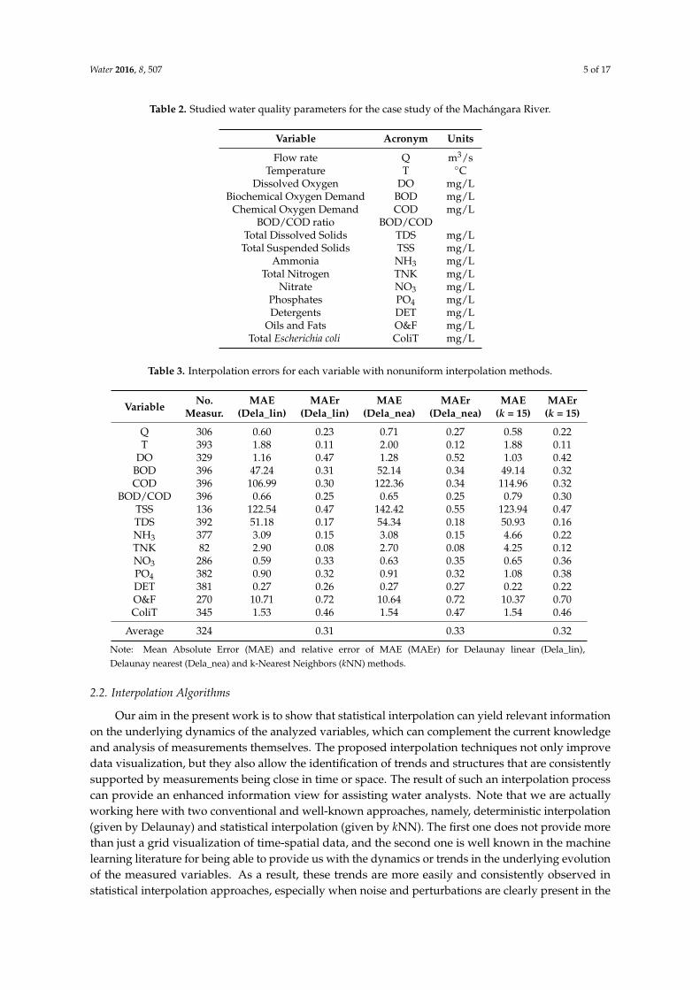
Table 2. Studied water quality parameters for the case study of the Machángara River.
Variable Acronym Units
Flow rate Q m3/sTemperature T ◦C
Dissolved Oxygen DO mg/LBiochemical Oxygen Demand BOD mg/L
Chemical Oxygen Demand COD mg/LBOD/COD ratio BOD/COD
Total Dissolved Solids TDS mg/LTotal Suspended Solids TSS mg/L
Ammonia NH3 mg/LTotal Nitrogen TNK mg/L
Nitrate NO3 mg/LPhosphates PO4 mg/LDetergents DET mg/L
Oils and Fats O&F mg/LTotal Escherichia coli ColiT mg/L
Table 3. Interpolation errors for each variable with nonuniform interpolation methods.
Variable No. MAE MAEr MAE MAEr MAE MAErMeasur. (Dela_lin) (Dela_lin) (Dela_nea) (Dela_nea) (k = 15) (k = 15)
Q 306 0.60 0.23 0.71 0.27 0.58 0.22T 393 1.88 0.11 2.00 0.12 1.88 0.11
DO 329 1.16 0.47 1.28 0.52 1.03 0.42BOD 396 47.24 0.31 52.14 0.34 49.14 0.32COD 396 106.99 0.30 122.36 0.34 114.96 0.32
BOD/COD 396 0.66 0.25 0.65 0.25 0.79 0.30TSS 136 122.54 0.47 142.42 0.55 123.94 0.47TDS 392 51.18 0.17 54.34 0.18 50.93 0.16NH3 377 3.09 0.15 3.08 0.15 4.66 0.22TNK 82 2.90 0.08 2.70 0.08 4.25 0.12NO3 286 0.59 0.33 0.63 0.35 0.65 0.36PO4 382 0.90 0.32 0.91 0.32 1.08 0.38DET 381 0.27 0.26 0.27 0.27 0.22 0.22O&F 270 10.71 0.72 10.64 0.72 10.37 0.70ColiT 345 1.53 0.46 1.54 0.47 1.54 0.46
Average 324 0.31 0.33 0.32
Note: Mean Absolute Error (MAE) and relative error of MAE (MAEr) for Delaunay linear (Dela_lin),Delaunay nearest (Dela_nea) and k-Nearest Neighbors (kNN) methods.
2.2. Interpolation Algorithms
Our aim in the present work is to show that statistical interpolation can yield relevant informationon the underlying dynamics of the analyzed variables, which can complement the current knowledgeand analysis of measurements themselves. The proposed interpolation techniques not only improvedata visualization, but they also allow the identification of trends and structures that are consistentlysupported by measurements being close in time or space. The result of such an interpolation processcan provide an enhanced information view for assisting water analysts. Note that we are actuallyworking here with two conventional and well-known approaches, namely, deterministic interpolation(given by Delaunay) and statistical interpolation (given by kNN). The first one does not provide morethan just a grid visualization of time-spatial data, and the second one is well known in the machinelearning literature for being able to provide us with the dynamics or trends in the underlying evolutionof the measured variables. As a result, these trends are more easily and consistently observed instatistical interpolation approaches, especially when noise and perturbations are clearly present in the

Water 2016, 8, 507 6 of 17
measurements. Note that, in this case, the interpolation process can be seen as a smoothing estimationprocess, which identifies the consistent trends and separates them from the system perturbations, asestimated by the model residuals.
In studies about multi-dimensional variables, it can be useful to search for dependencies amongthem; therefore, the construction of mathematical models should be able to describe those existingrelationships. Regression models can explain the dependency relationship between a response variableand one or more independent or explanatory variables in such a way that these models can estimatenew values from a new unobserved set of measurements from the explanatory variables.
The use of nonparametric regression is sometimes suitable when a response is difficult to obtainin terms of physical models or when the measuring methods are expensive. The main objective ofthe interpolation is to estimate one or more unknown independent variables from a given set ofsimultaneously measured samples from the independent variables and the response variable.
An intermediate goal in this work is to fill up the regular grid in the quantitative representationof water quality measurements at those times when no monitoring campaigns were conducted, and inthose spaces of rivers where there are no monitoring stations. The interpolation methods used in thiswork were Delaunay Triangulation and kNN.
2.2.1. Interpolation with Delaunay Triangulation
The interpolation with Delaunay triangulation has been used in digital cartography forthe generation of digital terrain models [16]. The starting point of this method is a cloud ofthree-dimensional (3D) points, usually irregularly spatial distributed, which allows us to representsurfaces digitally. This triangulation approximates surfaces by irregular and planar triangles thatconnect the 3D points. In this work, we do not use the 3D spatial coordinates of the points as inputspace, but instead we pursue a representation for two-dimensional input spaces given by the time andlocation (in terms of the distance along the river path), where a measurement was taken.
The Delaunay interpolation method is based on Voronoi diagrams and Delaunay triangulation,which uses the Euclidean distance as interpolation criterion [17]. Given two points in the spatio-temporalplane (x, t), denoted as p1 = (x1, t1) and p2 = (x2, t2), the Euclidean distance among them is
dist(p1, p2) :=√(x1 − x2)2 + (t1 − t2)2. (1)
Let P = {p1, p2, ..., pn} be a set of n distinct points (or sites) in the spatio-temporal plane.The Voronoi diagram of P is the subdivision of the plane in n cells (Figure 2a), one for each sitein P. The condition is that a point pe lies in the cell corresponding to a site pi if and only ifdist(pe, pi) < dist(pe, pj) for each pj ∈ P with j 6= i. The Voronoi diagram of P is denoted byVor(P), and it indicates only the edges and vertices of the subdivision pi [17]. Graph G has a nodefor every Voronoi cell equivalent for every site, and the union of external edges for each G conformsa polygon Pol.
Figure 2b shows the measurements (m axe) of a variable which forms a polyhedron of irregulartriangles where the measurements are the vertices. Note that bold uppercases are used to representpoints (vertices of irregular triangles which form a polyhedron) defined in the coordinates (x, t, m),while the projections of these vertices in the plane (x, t) are represented by bold lowercases.For example, samples represented by points A, B, and C form a triangle polyhedron, and whenit is projected in the plane (x, t), a new triangle with p1, p2, and p3 vertices is formed. The estimatedvalue, m̂E, at a new point E = (xE, tE), is obtained two-fold: (1) a Delaunay triangle, which enclosesthe point E, is found; and (2) m̂E is computed as the results of applying the values xE and tE in theplane equation defined by the points A, B and C in the linear interpolation, and as the mE value of thenearest neighbor vertex in the nearest interpolation.

Water 2016, 8, 507 7 of 17
2 4 6 8 101
2
3
4
5
6
7
8
9
10
Distance, x
Tim
e, t
G
pe
Region
pj
pi
Vor(P)
(a) (b)
Figure 2. Representation and nomenclature of the elements in our Delaunay interpolation: (a) Delaunaytriangulation and Voronoi diagram; and (b) obtaining a polyhedral from a set of sample points.
2.2.2. kNN Interpolation
The kNN rule is among the simplest statistical learning tools in density estimation, classification,and regression. Trivial to train and easy to code, the nonparametric algorithm is surprisinglycompetitive and fairly robust to errors when using cross-validation procedures [18]. The fittingis made by using only those measurements close to the target point pe. A function of weights assignedto each pi is based on the distance from pe.
The usual calculation methods of known distances are Euclidean, Manhattan, Minkowski,weighted Euclidean, Mahalanobis, and Cosine, among others. The Mahalanobis distance between twopoints p1 and p2 is defined as
distM(p1, p2) =
√(p1 − p2)
′∑−1(p1 − p2), (2)
where ∑ is the covariance matrix. Mahalanobis distance has advantageous properties compared tothe use of Euclidean distance, namely, it is invariant to changes in scale, and it does not depend onmeasurements units. By using matrix ∑−1, we consider correlations between variables and redundancyeffect. The estimation function of pe is represented by f̂ (pe), and it is estimated according to DistanceWeighted Nearest Neighbor algorithm as
f̂ (pe) =∑k
i=1 wi f (pi)
∑ki=1 wi
, (3)
where f (pi) represents the samples near pe, and wi is the weights function that is defined in terms ofMahalanobis distance as
wi =1
distM(pe, pi)2 . (4)
2.3. Performance Measures
The goal of any data-driven methodology is to estimate (learn) a useful model of the unknownsystem from available data. A criteria related to usefulness is the prediction accuracy (generalization),related to the capability of the model to provide accurate estimates for future data. In the learningproblem, the goal is to estimate a function by using a finite number of training samples. The availabilityof a finite number of training samples implies that any estimate of an unknown function is ofteninaccurate. In regression learning problems, we can obtain a measurement of the performance in

Water 2016, 8, 507 8 of 17
terms of the generalization capabilities of the model, with the goal of minimizing the empirical risk asdescribed below [19].
Given D = (xi, ti, mi)ni=1 as the training set, the pairs (xi, ti) are identified as inputs and (mi) as
outputs, where x represents the distance, t is time, and m is any water quality measurement. The basicgoal of supervised learning is to use the training set D to learn a function f̂ (in the hypothesis space H)that evaluates at a new pair (x, t) and estimates its associated value (m).
In order to measure the quality of f̂ function, we use a loss function denoted by l( f̂ , D).The estimation for a given (x, t) is f̂ (x, t), and the true value is (m). One of the loss functionsused in this paper is the absolute error loss, which can be written as
l( f̂ , D) = | f̂ (x, t)−m|. (5)
Given a function f̂ , a loss function l, and a probability distribution g over (x, t), the generalizationerror (also called actual error) of f̂ is defined as
Rgen[ f̂ ] = EDl( f̂ , D), (6)
which is also the expected loss on a new example which has been randomly drawn from the distribution.In general, we do not know g and cannot compute Rgen[ f̂ ]. Therefore, we use the empirical error
(or risk) of f̂ as
Remp[ f̂ ] =1n
n
∑i=1
l( f̂ , Di), (7)
and when the loss function is the absolute error loss, the empirical error is
Remp[ f̂ ] =1n
n
∑i=1| f̂ (xi, ti)−mi|, (8)
which is the risk function used in this work, but from now on, we will use for it MAE, [20,21],
MAE = Remp[ f̂ ]. (9)
Therefore, predictive performance of regression models can be estimated by using standardmetrics such as the regression MAE.
The loss function can be calculated using the validation data, which are sensitive to the choice ofthe validation set. This is a problem when the data set is small, and, in these cases, the cross validationtechnique allows more efficient use of available data [22]. For statistical result evaluation, the k-foldcross-validation method was used here, where data are partitioned into k subsets or folds, D1, D2, ..., Dkthat are generally of the same size. A Di partition serves for testing and the remaining ones for training.On the first iteration, D1 is used for the test and the remaining D2, D3, ..., Dk for training. Therefore,k iterations are carried out until Dk are tested, and the others are used for training. Each data setsample is used once for training and after that just for testing. Leave-one-out is a special case of k-foldcross-validation where k is set to number of initial tuples. That is, only one sample is “left out” at a timefor the test set. Therefore, in this work, we have used Leave-One-Out for the estimation of the MAEin the two interpolation algorithms used here, called Delaunay (either with linear or with nearestcriterion) and kNN (with Mahalanobis distance).
2.4. Behavior of Interpolation Errors
Given that the interpolation error depends on the analyzed variable, the number of measurements,and the interpolation method, it is advisable to use a relative error of the MAE value. Following [23],in this work, we use
MAEr =MAE
u, (10)

Water 2016, 8, 507 9 of 17
where MAEr is the relative error of MAE, and u is the average value of each variable of water quality.On the other hand, the MAE obtained by the kNN algorithm for different variables of water
quality depends on the k parameter, which takes different values due to the nature of each variable.
3. Results
In this section, the performance of the interpolation algorithms is analyzed, based on data frommonitoring campaigns conducted in irregular time periods and non-uniform distances betweenstations. This is a usual situation, which can be due to logistical problems or bad weather conditions,among other factors.
3.1. Free Parameter k and Algorithm Comparisons
In order to establish a comparison between deterministic and statistical interpolation, we startedby scrutinizing the value of k to be used as a free parameter in the kNN algorithm. Figure 3 shows thechanges of MAEr with respect to k. It can be observed that we almost always need few neighbors foryielding a value close to the minimum MAE. As errors decrease very slowly after some point, and forcomputational simplicity, we decided to use k = 15 for all the kNN variable models. On the other hand,Figure 4 shows the variability of MAEr with respect to the normalized number of measurements. It canbe observed that MAEr is reduced by increasing the number of available samples, though a extremelyreduced number of available samples sometimes can yield an apparently reduced error, probably dueto the poor representation of the dynamics in these cases.
Figure 3. Behavior of MAEr for different k values.
Figure 4. MAEr for different normalized numbers of measurements. DL-MAEr is for Delaunay linear,DN-MAEr is for Delaunay nearest, and kNN-MAEr is for kNN method.

Water 2016, 8, 507 10 of 17
Table 3 presents the MAE of each variable obtained with each interpolation algorithm (withk = 15 for kNN). Note that MAE values are significantly different among water quality variables, andbecause of that, we also included the relative MAE (MAEr). The average value of MAEr was 0.31 forDelaunay-linear, 0.33 for Delaunay-nearest, and 0.32 for kNN, which, roughly speaking, shows thatabout two thirds of the variations are jointly explained by the underlying dynamics.
We also analyzed which interpolation method provides with the best estimation of the dynamics(i.e., trends or patterns) for the observed variables. Figure 5a shows the interpolation of NH3 withDelaunay-linear, which also resembles the one obtained by applying Delaunay-nearest shown inFigure 5b. Both interpolation techniques present a typical step-like view of the interpolated variable.On the other hand, Figure 5c shows the interpolation results of NH3 with the kNN method. In thislater case, data dynamics are better observed because of the improved smoothing, allowing us toeasily see spatial and temporal trends. As another example, Figure 5d shows PO4 interpolation withDelaunay-linear, while Figure 5e shows a noticeable smoothing when the kNN method is used. Again,the kNN technique shows more clearly some spatial trends for the PO4 variable. Figure 5f showsanother example of the ColiT interpolation when using the kNN method, displaying the dynamicsof some trends and consistent peaks on it. Interpolation errors of each method on each variable aredetailed in Table 3.
Figure 6a shows the rainfall in the study area during the period 2002–2007 recorded by a nearbyweather station. This information is included for comparison of some of the water quality variables inthe same figure. The variables in Figure 6 are Q, T, DO, BOD/COD, and TNK, whose representationsare drawn in elevation view for better visual observation of their spatio-temporal dynamics. As far asFigures 5 and 6 show eight variables of a total of 15 water quality parameters of Machángara River,the seven remaining variables that are not represented are BOD, COD, TDS, TSS, NO3, DET, andO&F. It should be noted that those representations exhibit a similar smoothing compared to the eightvariables previously represented when using the kNN method.
(a) (b)
(c) (d)
Figure 5. Cont.

Water 2016, 8, 507 11 of 17
(e) (f)
Figure 5. Results of Delaunay and kNN Interpolation methods: (a) NH3 with Delaunay linear; (b) NH3
with Delaunay nearest; (c) NH3 with kNN; (d) PO4 with Delaunay linear; (e) PO4 with kNN; and(f) ColiT with kNN.
500 1000 1500 2000
20
40
60
80
100
120
140
160
180
200
time, days
Rain,(m
m/m
2)
(a) (b)
(c) (d)
(e) (f)
Figure 6. Spatio-temporal variation: (a) rainfall level in Quito from 2002 to 2007 at ‘La Tola’ monitoringstation; (b) Q; (c) DO; (d) T; (e) BOD/COD; (f) TNK.

Water 2016, 8, 507 12 of 17
3.2. Analysis of the Spatio-Temporal Model Residuals
In the previous section, it was not clear which interpolation method performed better justin terms of averaged error. For a fair benchmarking, we proposed making an analysis on thespatio-temporal distribution of the model residuals. Taking into account that the leave-one-out residualwas obtained for each method in each sample, Figure 7 displays the difference in terms of AbsoluteError (AE) between kNN and Delaunay methods for six different variables. Blue markers representthe difference of AE (∆AE = AEDelaun − AEkNN) when Delaunay obtains worse performances thankNN (i.e., for the case AEDelaun − AEkNN > 0) and red markers are shown otherwise (i.e., for the case∆AE = AEkNN − AEDelaun).
(a) (b)
(c) (d)
(e) (f)
Figure 7. Spatio-temporal distributions for |∆AE| = |AEkNN − AEDelaun|: (a) O&F; (b) DET;(c) BOD/COD; (d) DO; (e) NO3; and (f) PO4.

Water 2016, 8, 507 13 of 17
From Figure 7, several ideas can be summarized. Although the largest differences (due to outliersor atypical measurements) can be obtained for both methods in some cases, as seen in (e,f), outliers arebetter treated by kNN in most of the cases, as seen in (a–d). In addition, kNN works better for somegiven variables, which are (a,b), and (d), whereas its performance can degrade compared to Delaunayin cases such as (e), or it can be similar in cases such as (f).
If we compare these results with the observations and estimation in Figure 5, it can be concludedthat kNN works better for outliers and for slow-dynamics variables with smooth changes, whereasfast-dynamics variables can be over-smoothed by this method, and, then its model residuals are notcapable of improving the trivial interpolation made by Delaunay.
3.3. Evolution of Water Quality Measurements
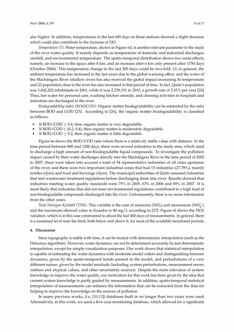
Flow rate (Q). Figure 6b shows the Machángara River flow rate, and it depends on several factors,namely, the tributaries formed by streams coming from the Pichincha volcano (Quito is a city locatedbetween the slopes of a volcano and the Machángara River), the runoffs due to rainfall in the upperbasin of Quito, and the wastewater from domestic and industrial discharges in the central and thesouthern parts of the city. Additionally, Quito does not have independent pipes for domestic, industrial,or runoff water, but rather this wastewater is a composition of all them. Figure 8 represents the averageof the maximum values of flow rates for each year from 2002 to 2007 of a total of 19 major tributariesupstream of the Machángara River. Figure 8 shows two peaks (m3/s) that are present at about 500 days(2003) and 1250 days (2005), whereas we can see a decrease of the flow rate at 800 days (2004), likelydue to the scarcity of rains. Although this represents an annually averaged measurements of flowrates, this plot and the rainfall one (Figure 6a) could better explain the evolution of water dischargesinto the river as shown in Figure 6b. In this last figure, two flow rate peak at about 500 and 1500 daysare displayed, which could be due to rainfall and flow rate of the Machángara River’s tributaries.The changes in the total flow could affect the behavior of other water quality characteristics.
Figure 8. Average of the maximum values of flow rates for each year (from 2002 to 2007) depictedwhen time is shown in days.
Dissolved Oxygen (DO). Figure 6c shows that DO increases in space after about 2 km, and in timeespecially after January 2006 (1460 days). Figure 6d shows a temperature increase in the river´s water atthe last station (9.49 km). As temperature increases, oxygen solubility decreases. Therefore, dissolvedoxygen should be lower (see Figure 6c). In addition, it can be observed that DO increases during thelast 600 days between ST3 and ST5. In this section, the Machángara River has a lot of stones and debris.This condition may cause an intensive crush of water against these materials, hence producing a largeamount of small water bubbles. It is well known that as water bubbles get smaller, the liquid–gasinterface area increases, and thus oxygen can be dissolved at a higher rate. As a result, DO should be
Water 2016, 8, 507 14 of 17
also higher. In addition, temperatures in the last 600 days in those stations showed a slight decreasewhich could also contribute to the increase of DO.
Temperature (T). Water temperature, shown in Figure 6d, is another relevant parameter in the studyof the river water quality. It mainly depends on temperature of domestic and industrial discharges,rainfall, and environmental temperature. The spatio-temporal distribution shows two main effects,namely, an increase in the space after 8 km, and an increase after 6 km only present after 1750 days(October 2006). This temperature change in the last 300 days could be two-fold: (1) in general, theambient temperature has increased in the last years due to the global warming effect, and the water ofthe Machángara River (shallow river) has also received the global impact increasing its temperature;and (2) population close to the river has also increased in that period of time. In fact, Quito’s populationwas 1,842,202 inhabitants in 2001, while it was 2,239,191 in 2010, a growth rate of 2.41% per year [24].Thus, hot water for personal care, washing kitchen utensils, and cleaning activities in hospitals andindustries are discharged in the river.
Biodegradability index (BOD/COD). Organic matter biodegradability can be estimated by the ratiobetween BOD and COD [25]. According to [26], the organic matter biodegradability is classifiedas follows:
• If BOD/COD ≥ 0.4, then organic matter is very degradable.• If BOD/COD ∈ (0.2, 0.4), then organic matter is moderately degradable.• If BOD/COD ≤ 0.2, then organic matter is little degradable.
Figure 6e shows the BOD/COD ratio where there is a relatively stable value with distance. In thetime period between 800 and 1200 days, there were several industries in the study area, which usedto discharge a high amount of non-biodegradable liquid compounds. To investigate the pollutionimpact caused by their water discharges directly into the Machángara River in the time period of 2002to 2007, there were taken into account a total of 54 representative industries of all cities upstreamof the river, and there were two important industrial zones that had 15 industries (27.78%), mainlytextiles (dyes) and food and beverage (dyes). The municipal authorities of Quito assessed industriesthat met wastewater treatment regulations before discharging them into river. Results showed thatindustries meeting water quality standards were 75% in 2005, 63% in 2006 and 69% in 2007. It ismost likely that industries that did not meet environmental regulations contributed to a high load ofnon-biodegradable compounds discharged into the river. Unfortunately, there is no more informationfrom the other years.
Total Nitrogen Kjeldahl (TNK). This variable is the sum of ammonia (NH3) and ammonium (NH+4 ),
and the maximum allowed value in Ecuador is 40 mg/L according to [27]. Figure 6f shows the TKNvariation, which is in this case constrained to about the last 400 days of measurements. In general, thereis a sustained level near the limit, both below and above it, for most of the available monitored periods.
4. Discussion
Since topography is stable with time, it can be treated with deterministic interpolation (such as theDelaunay algorithm). However, water dynamics can not be determined accurately by just deterministicinterpolation, except for simple visualization purposes. Our work shows that statistical interpolationis capable of estimating the water dynamics with moderate model orders and distinguishing betweendynamics, given by the spatio-temporal trends present in the model, and perturbations of a verydifferent nature, given by the model residuals (including system perturbations, measurement errors,outliers and atypical values, and other uncertainty sources). Despite the main relevance of systemknowledge to improve the water quality, our motivation for this work has been given by the idea thatcurrent system knowledge is partly guided by measurements. In addition, spatio-temporal statisticalinterpolation of measurements can enhance the information that can be extracted from the data forhelping to improve the knowledge on the sources of pollution.
In many previous works, (i.e, [10,13]) databases built in no longer than two years were used.Alternatively, in this work, we used a five-year monitoring database, which allowed for a significant
Water 2016, 8, 507 15 of 17
amount of records of water quality parameters similar to the work described in [11,28]. Our databaseconsisted of 64 monitoring campaigns and 4867 water quality records. This allowed us to buildinterpolation grids with a spatial resolution of 400 m and a temporal resolution of one day. We obtaineda simple to adjust k value by using the kNN algorithm where a stable and close to minimum MAEwas achieved. This simplicity allowed us to construct a spatio-temporal grid with the measured waterquality parameters and the data processed by nonuniform interpolation methods.
When analyzing the model residuals for comparison between kNN and Delaunay interpolation,we found that kNN estimation provides acceptable estimation of the variable dynamics in the presenceof atypical samples, and in slow-dynamics variables, whereas it can present some over-smoothingeffects on fast-changing variables. This suggests that, whereas conventional interpolation algorithmscan provide acceptable estimation capabilities, further interpolation algorithms should be designed forovercoming their current limitations.
The MAE obtained for phosphates in [11] was 0.466 by using Bayesian methods, while, in thiswork, it is 1.08 when using kNN. This difference could be due to different water quality datasets, and,therefore, it does not stand for a straight comparison. However, we consider this previous work ascomparable to ours in terms of estimation techniques. While [29] presents only the nitrate dynamicsof the Turia River (Valencia Spain), in this paper we show nitrogen and other variables with goodspatio-temporal resolution.
5. Conclusions
The proposed spatio-temporal analysis of water quality measurements using interpolationalgorithms for measurements from campaigns can provide useful and relevant information on theirdynamics, in the sense of trends and structure. This can complement the current knowledge from theexperience and from physical models and help extend it. New methods of interpolation are encouragedto overcome the limitations of conventional interpolation methods in this scenario. While a secondarytarget, visualization of these trends provides a way of visually inspecting the data models, andresidual visualization can provide data quality measurement of the estimation model under use andits uncertainty.
Water quality values resulting from the application of the smoothing interpolation algorithms,especially for those places that are difficult to reach and for irregular time periods, can also providerelevant information for designers of wastewater treatment plants. For example, it can be used forother sections of the Machángara River and make studies about inter-dependence between waterquality variables, (e.g., nitrates and phosphates).
The database used in this work corresponds to a period between 2002 and 2007, a time periodwhen few hydrology monitoring stations existed for capturing the rainfall in the city or near the studyzone. Even today, there are no more water quality monitoring stations than those ones constructed in2002–2007. The major contributors of wastewater in the Machángara River are domestic and industrialdischarge, and furthermore, in our city, there were no separate pipes for rainfall and wastewater(and still today there are not yet any). For these reasons, in our study, we especially missed havingdenser spatial sampling rates (stations), as well as the always desirable increase in time sampling rates(measurement campaigns).
A limitation of this study is the lack of time records (the hour of the day) in which the watersamples were collected and analyzed. Variables such as water temperature, concentrations of detergents,phosphates, oils and fats are not constant during the 24 h, since they depend on discharge of domesticand industrial wastewater and meteorological conditions. Therefore, conducting an extended studyconsidering smaller time periods between samples for 24 h each day could provide us with usefulinformation for studies on the uses of water than could be characterized by time and population type.
Acknowledgments: This work was supported in part by the Universidad de las Fuerzas Armadas ESPE underGrant 2015-PIC-004 and has also been partly supported by Research Grants PRINCIPIAS (TEC2013-48439-C4-1-R)and FINALE (TEC2016-75161-C2-1-R) from the Spanish Government and PRICAM (S2013/ICE-2933) from

Water 2016, 8, 507 16 of 17
Comunidad de Madrid. The authors thank the Metropolitan Water Company of Quito, Ecuador, for providing theMachángara River water quality data.
Author Contributions: Iván P. Vizcaíno, Enrique V. Carrera, José Luis Rojo-Álvarez and Luis H. Cumbal conceivedand designed the experiments. Iván P. Vizcaíno, Sergio Muñoz-Romero and Margarita Sanromán-Junqueraperformed the experiments. Enrique V. Carrera, Luis H. Cumbal and José Luis Rojo-Álvarez supervised theexperiments. Iván P. Vizcaíno wrote the paper, and all authors contributed with changes in all sections.
Conflicts of Interest: The authors declare no conflicts of interest.
References
1. Van der Perk, M. Soild and Water Contamination from Molecular to Catchment Scale, 1st ed.; Taylor andFrancis/Balkema: Leiden, The Netherlands, 2006.
2. Duan, W.; Takara, K.; He, B.; Luo, P.; Nover, D.; Yamashiki, Y. Spatial and temporal trends in estimates ofnutrient and suspended sediment loads in the Ishikari River, Japan, 1985 to 2010. Sci. Total Environ. 2013,461–462, 499–508.
3. Duan, W.; He, B.; Takara, K.; Luo, P.; Nover, D.; Sahu, N.; Yamashiki, Y. Spatiotemporal evaluation of waterquality incidents in Japan between 1996 and 2007. Chemosphere 2013, 93, 946–953.
4. Heinke, G.G.; Ingeniería Ambiental, 2nd ed.; Prentice Hall Hispanoamericana, S.A.: Upper Saddle River, NJ,USA, 1999; pp. 421–424.
5. Tebbutt, T.H.Y. Principles of Water Quality Control, 5th ed.; Butterworth-Heinemann an Imprint of ElsevierScience: Oxford, UK, 1998; pp. 21–22.
6. Corcoran, E.; Nellemann, C.; Baker, E.; Bos, R.; Osborn, D. Sick Water? The Central Role of WastewaterManagement in Sustainable Development; Savelli, H., Ed.; Birkeland Trykkeri AS: Birkeland, Norway, 2010.
7. Meneses, M.; Concepción, H.; Vilanova, R. Joint Environmental and Economical Analysis of WastewaterTreatment Plants Control Strategies: A Benchmark Scenario Analysis. Sustainability 2016, 8, 360.
8. Thangarajan, M. Groundwater Resource Evaluation, Augmentation, Contamination, Restoration, Modeling andManagement; Springer: Dordrecht, The Netherlands; Capital Publishing Company: New Delhi, India, 2007;pp. 12–17.
9. Taalohi, M.; Tabatabaee, H. Predicting Bar Dam Water Quality using Neural-Fuzzy Inference System. Indian J.Fundam. Appl. Life Sci. 2014, 4, 630–636.
10. Li, S.; Liu, W.; Gu, S.; Cheng, X.; Xu, Z.; Zhang, Q. Spatio temporal dynamic of nutrients in the upper HanRiver basin, China. Hazard. Mater. 2009, 162, 1340–1346.
11. Serre, M.; Carter, G.; Money, E. Geostatistical space/time estimation of water quality along the Raritan riverbasin in New Jersey. Dev. Water Sci. 2004, 55, 1839–1852.
12. Duan, W.; He, B.; Nover, D.; Yang, G.; Chen, W.; Meng, H.; Zou, S.; Liu, C. Water Quality Assessment andPollution Source Identification of the Eastern Poyang Lake Basin Using Multivariate Statistical Methods.Sustainability 2016, 8, 133.
13. Gomez, M.; Herrera S.; Solé, D.; García-Calvo, E.; Fernández-Alba, A. Spatio temporal evaluation of organiccontaminants and their transformation products along a river basin affected by urban, agricultural andindustrial pollution. Sci. Total Environ. 2012, 420, 134–145.
14. Empresa Pública Metropolitana de Agua Potable Quito. Estudios de Factibilidad y Diseños Definitivos delPlan de Descontaminación de los Ríos de Quito Informe No.1 “Revisión de la Información Existente y Diagnóstico”;Technical Report; Empresa Pública Metropolitana de Agua Potable Quito: Quito, Ecuador, 2009.
15. Municipio del Distrito Metropolitano de Quito. Plan de Desarrollo 2012–2022. Consejo Metropolitano dePlanificación. Quito, Ecuador; Municipio del Distrito Metropolitano de Quito: Quito, Ecuador, 2011; pp. 14–26.
16. Priego de los Santos, J.; Porres de la Haza, M. La Triangulación Delaunay Aplicada a los Modelos Digitalesdel Terreno; Universidad Politécnica de Valencia: Valencia, Spain, 2002; pp. 1–8.
17. De-Berg, M.; Cheong, O.; Van-Kreveld, M.; Overmars, M. Computational Geometry, Algorithms and Applications,3rd ed.; Springer: Berlin/Heidelberg, Germany, 2008; pp. 196–198.
18. Karl, S.; Truong, Q. An Adaptable k-Nearest Neighbors Algorithm for MMSE Image Interpolation.IEEE Trans. Image Process. 2009, 18, 1976–1987.
19. Cherkassky, V.; Mulier, F. Learning From Data: Concepts, Theory, and Methods, 2nd ed.; Wiley-Interscience:Hoboken, NJ, USA, 2007; pp. 61–64.

Water 2016, 8, 507 17 of 17
20. Elisseeff, A.; Pontil, M. Leave-one-out error and stability of learning algorithms with applications.Mach. Learn. Res. 2002, 55, 71–97.
21. Mukherjee, S.; Niyogi, P.; Poggio, T.; Rifkin, R. Statistical Learning: Stability Is Sufficient For Generalization andNecessary and Sufficient for Consistency of Empirical Risk Minimization; Massachusetts Institute of Technology:Cambridge, MA, USA, 2004.
22. Rogers, S.; Girolami, M. A First Course in Machine Learning, 1st ed.; Chapman & Hall/CRC: New York, NY,USA, 2011; pp. 29–31.
23. Uriel-Jiménez, E.; Aldás-Manzano, J. Análisis Multivariante Aplicado; Thomson Editores Spain Paraninfo S.A.:Madrid, Spain, 2005; pp. 56–57.
24. Instituto Nacional de Estadísticas y Censos. Base de Datos Censo 2010; INEC: Quito, Ecuador, 2010.25. Tien, M.; Lai, J.; Jin, H. Estimating the Biodegradability of Treated Sewage Samples Using Synchronous
Fluorescence Spectra . Sensors 2011, 11, 7382–7394.26. Martín, I.; Betancourt, J. Guía Sobre Tratamientos de Aguas Residuales Urbanas para PequeñOs NúCleos de
PoblacióN. Mejora de la Calidad de los Efluentes, 1st ed.; Daute Diseño, S.L.: Las Palmas, Spain, 2006.27. Presidencia de la República del Ecuador. Norma de Calidad Ambiental y de Descarga de Efluentes: Recurso Agua;
Technical Report; Presidencia de la República del Ecuador: Quito, Ecuador, 2012.28. Clement, L.; Thas, O.; Vanrolleghem, P.A.; Ottoy, J.P. Spatio-temporal statistical models for river monitoring networks.
Water Sci. Technol. 2006, 53, 9–15.29. Capella, J.; Bonastre, A.; Ors R.; Peris, M. In line river monitoring of nitrate concentration by means of
a Wireless Sensor Network with energy harvesting. Sens. Actuators 2013, 177, 419–427.
© 2016 by the authors; licensee MDPI, Basel, Switzerland. This article is an open accessarticle distributed under the terms and conditions of the Creative Commons Attribution(CC-BY) license (http://creativecommons.org/licenses/by/4.0/).