spe 141677 use of approximate dynamic programming for...

SPE 141677

Use of Approximate Dynamic Programming for Production Optimization

Zheng Wen, Louis J. Durlofsky, SPE, Benjamin Van Roy, Khalid Aziz, SPE, Stanford University

Copyright 2011, Society of Petroleum Engineers

This paper was prepared for presentation at the 2011 SPE Reservoir Simulation Symposium held in Woodlands, Texas, U.S.A., 21-23 February 2011.

This paper was selected for presentation by an SPE Program Committee following review of information contained in an abstract submitted by the author(s). Contents of the

paper, as presented, have not been reviewed by the Society of Petroleum Engineers and are subject to correction by the author(s). The material, as presented, does not

necessarily reflect any position of the Society of Petroleum Engineers, its officers, or members. Papers presented at SPE meetings are subject to publication review by Editorial

Committees of the Society of Petroleum Engineers. Electronic reproduction, distribution, or storage of any part of this paper for commercial purposes without the written consent

of the Society of Petroleum Engineers is prohibited. Permission to reproduce in print is restricted to an abstract of not more than 300 words; illustrations may not be copied. The

abstract must contain conspicuous acknowledgment of SPE copyright.

Abstract

In production optimization, we seek to determine the well settings (bottomhole pressures, flow rates) that maximize an objectivefunction such as net present value. In this paper we introduce and apply a new approximate dynamic programming (ADP) algorithmfor this optimization problem. ADP aims to approximate the global optimum using limited computational resources via a systematicset of procedures that approximate exact dynamic programming algorithms. The method is able to satisfy general constraints such asmaximum watercut and maximum liquid production rate in addition to bound constraints. ADP has been used in many applicationareas, but it does not appear to have been implemented previously for production optimization. The ADP algorithm is applied to two-dimensional problems involving primary production and water injection. We demonstrate that the algorithm is able to provide clearimprovement in the objective function compared to baseline strategies. It is also observed that, in cases where the global optimum isknown (or surmised), ADP provides a result within 1-2% of the global optimum. Thus the ADP procedure may be appropriate forpractical production optimization problems.

Introduction

Many optimization algorithms have been applied to maximize reservoir performance. Most of these optimization algorithms can beclassified into two categories: gradient-based/direct-search [20, 15] and global stochastic search [13, 1, 7]. Both classes of optimizationalgorithms face limitations: gradient-based and direct-search algorithms settle for local optima, while global stochastic search algorithmssuch as genetic algorithms typically require many function evaluations for convergence, and even then there is no assurance that theglobal optimum has been found.

In principle, one can formulate production optimization as a nonlinear optimal control problem and find a global optimum usingdynamic programming (DP) [2]. The key idea in DP is to decompose the optimization problem into a sequence of sub-problems, eachrepresenting optimization of a control action at one point in time. These sub-problems are related through the value function, whichmaps the system state to the net present value of future revenues. Once the value function is computed, the optimal control action at eachtime can be found by solving a sub-problem at that time. In general, these sub-problems are much simpler than the original optimizationproblem; in many cases, a global optimum of each sub-problem can be efficiently computed.

For problems of practical scale, the computational requirements of DP become prohibitive due to the curse of dimensionality. Inparticular, time and memory requirements typically grow exponentially with the number of state variables. Approximate dynamicprogramming (ADP) aims to address this computational burden by efficiently approximating the value function (see [3, 25, 19] for moreon ADP). The result is an approximate value function, which is typically represented by a linear combination of a set of predefinedbasis functions. ADP algorithms provide methods for computing the coefficients associated with these basis functions. ADP hasbeen successfully applied across a broad range of domains such as asset pricing [23, 18, 24], transportation logistics [21], revenuemanagement [26, 10, 27], portfolio management [14, 12], and even to games such as backgammon [22].

In this paper, we introduce a new ADP algorithm for petroleum reservoir production optimization. We apply our algorithm to single-

2 Use of Approximate Dynamic Programming for Production Optimization SPE 141677

phase and multiphase problems with simple or general well and production constraints and compare performance to that achieved usingvarious baseline strategies. As we will show, ADP performs well relative to the baseline results for the problems considered.

Performance aside, it is worth noting that for reservoir production problems, our ADP algorithm offers some advantages relative toalternative optimization techniques. For example, ADP can readily handle general (nonlinear) constraints, such as maximum watercut,which are not straightforward to handle with some algorithms. In addition, although our proposed ADP algorithm does include non-deterministic components (specifically constraint sampling, as described below), the ADP algorithm is otherwise non-stochastic, yetit searches for the global optimum. This distinguishes it from other global search algorithms that have been applied to productionoptimization.

This paper is organized as follows. First, we formulate a dynamic optimization model for the reservoir production problem. Second,we describe our ADP algorithm for reservoir production, focusing on how we construct and select basis functions and how we computethe coefficients of these basis functions. Third, we discuss the computational demands of the ADP algorithm in terms of the number ofsimulations required. Fourth, we present simulation results and compare the performance of the ADP algorithm to various baselines.We conclude with a summary.

Dynamic Optimization Model

We represent the discrete system of reservoir flow equations as a system of ordinary differential equations:

dx(t)/dt = F (x(t),u(t)) , (1)

subject to an initial condition x(0) = x0 and instantaneous constraints S(x(t),u(t)) ≤ 0. Here x(t) and u(t) denote the reservoir statesand the control action at time t, respectively. Typically, x includes the pressure and saturation of each grid block and u encodes BHPsand/or flow rates of the injection/production wells (or well groups). The constraints S(x(t),u(t)) ≤ 0 restrict the state and controlaction at time t. Constraints in reservoir production problems typically include upper/lower bounds on BHPs, upper/lower bounds onflow rates of components (oil/water/gas), and maximum watercut or gas cut of production wells or well groups.

We also assume that at time t, a payoff accumulates at a rate given by an instantaneous payoff function L(x(t),u(t)) that dependson the state x(t) and control action u(t). A widely used instantaneous payoff function is

L(x(t),u(t)) = revenue from producing oil − (cost for producing water + cost for injecting water) . (2)

Our objective is to maximize the net present value (NPV) of future payoffs� T0 e−αtL (x(t),u(t)) dt, where α ≥ 0 is the continuous-

time discount rate.In most reservoir production problems, the termination time T is large enough so that the difference between the NPV of the

cumulative profit,� T0 e−αtL (x(t),u(t)) dt, and its infinite horizon approximation,

�∞0 e−αtL (x(t),u(t)) dt, is sufficiently small.

Moreover, it is well known that there exists a stationary policy u∗(t) = µ∗ (x(t)) maximizing the infinite horizon discounted objective.As we will see later, the existence of a stationary globally optimal policy µ∗ simplifies our ADP algorithms. For this reason, we willfocus on solving the infinite horizon dynamic optimization problem:

max{u(t),t≥0}

� ∞

t=0e−αt

L(x(t),u(t))dt

s.t. dx(t)/dt = F (x(t),u(t)) (3)x(0) = x0

S (x(t),u(t)) ≤ 0.

Approximate Dynamic Programming Algorithms for Reservoir Production

In this section, we develop an optimization algorithm based on Approximate Dynamic Programming (ADP) for the dynamic op-timization model presented above. We first review Dynamic Programming (DP) and Approximate Dynamic Programming (ADP),then describe how we construct basis functions for reservoir production problems, then introduce a linear programming (LP) basedapproach to compute the basis-function coefficients, then discuss the computation of globally-optimal controls (or near globally-optimal controls), and finally describe two advanced techniques – adaptive basis function selection and bootstrapping – to improvealgorithm performance. Throughout this section, we assume that we have access to a reservoir simulator, which can numerically solvedx(t)/dt = F (x(t),u(t)).

Review of Dynamic Programming

Dynamic programming (DP) offers a class of optimization algorithms that decompose a dynamic optimization problem into asequence of simpler sub-problems. At each time t, an optimal control action u∗(t) is computed by solving one sub-problem. Thesesub-problems are coordinated across time through a value function denoted by J∗. The value function captures the future impact of the

SPE 141677 Wen, Durlofsky, Van Roy and Aziz 3

current action; the algorithm must balance immediate payoff against future possibilities. In our model, the value function is defined by:

J∗(x0) = maxu(t),t≥0

�∞t=0 e

−αtL(x(t),u(t))dt

s.t. dx(t)/dt = F (x(t),u(t))x(0) = x0

S (x(t),u(t)) ≤ 0.

(4)

Note that J∗(x0) is the maximum net present value starting from state x0 at time 0. Further, given the time homogeneity of our model,the value J∗(x(t)) at any time t and for any state x(t) is the maximum net present value of payoffs that can be accumulated starting atthat time and state.

Given the value function J∗ and current state x(t), an optimal control action at time t can be selected by solving the followingoptimization problem [2]:

maxu

L (x(t),u) + F (x(t),u)T ∇J∗ (x(t)) (5)

s.t. S(x(t),u) ≤ 0,

where ∇J∗ is the gradient of J∗. Note that this problem decouples the choice of control action at time t from that at all other times. Itis in this sense that DP decomposes the dynamic optimization problem into simpler sub-problems through use of the value function. Aswe will see later, for reservoir production problems, the sub-problem (5) can be solved efficiently.

In light of the relative ease of generating optimal control actions given the value function, the challenge in optimizing reservoirproduction using DP (or ADP) reduces to the computation of the value function. As discussed in [12], the optimal value function for acontinuous-time optimal control problem can in principle be computed by solving the Hamilton-Jacobi-Bellman (HJB) equation:

maxu:S(x,u)≤0

�L(x,u) + F (x,u)T∇J(x)− αJ(x)

�= 0, (6)

which is a nonlinear partial differential equation, or alternatively by solving an infinite dimensional linear program (LP):

minJ

�J(x)π(dx)

s.t. L(x,u) + F (x,u)T∇J(x)− αJ(x) ≤ 0 ∀x,u such that S(x,u) ≤ 0, (7)

where π is a probability measure chosen with exhaustive support such that that the integral of J∗ is finite. This LP poses an infinitenumber of decision variables and an infinite number of constraints since there is one decision variable J(x) per state x and there is oneconstraint S(x,u) ≤ 0 per state-action pair (x,u).

In most reservoir production problems of practical interest, solving the HJB equation (6) or the LP (7) exactly is impossible, as thiswould require computing and storing J∗ for each state in a continuous state space. Even if we were to discretize the state space byquantizing each state variable into multiple discrete values, the number of discrete states would grow exponentially as a function of D,the dimension of the state space, again making storage and computation impractical.

In a few special cases, the value function assumes a special structure which facilitates efficient computation and storage. This is thecase, for example, with single-phase reservoir models with no constraints on control actions and an instantaneous payoff function thatis quadratic in state and control action. In this context, the value function is itself quadratic and the problem reduces to one of linear-quadratic control (LQ). Such problems are well known to be tractable. For more realistic problems, involving for example multiphaseflow, the reservoir dynamics are nonlinear and computing the value function exactly is infeasible.

Approximate Value Function

One way to overcome the curse of dimensionality is to approximate the value function. As is common in ADP, we will approximatethe value function of our dynamic optimization model in terms of a linear combination of a selected set of basis functions:

J∗(x) ≈ J(x) =

K�

k=0

rkφk(x), (8)

where φk(·), k = 0, · · · ,K is a set of basis functions, and the rk’s are their respective coefficients. Replacing the exact value functionJ∗ with the approximation J when solving each sub-problem (5) results in a control strategy u = µ(x). Of course µ is not in generalequal to µ∗, and thus is not in general a global optimum. However, if J is “close” to J∗, the use of controls µ will provide performancethat is “close” to the global optimal. ADP algorithms aim to obtain a near-optimal strategy µ through appropriate (application-specific)approximation of the value function.

Our ADP algorithm proceeds as follows:


1. Construct a set of basis functions φk(·), k = 0, · · · ,K.

2. Compute the coefficients rk of the basis functions.

3. Compute near-optimal control actions u using the approximate value function J by solving sub-problem (5).

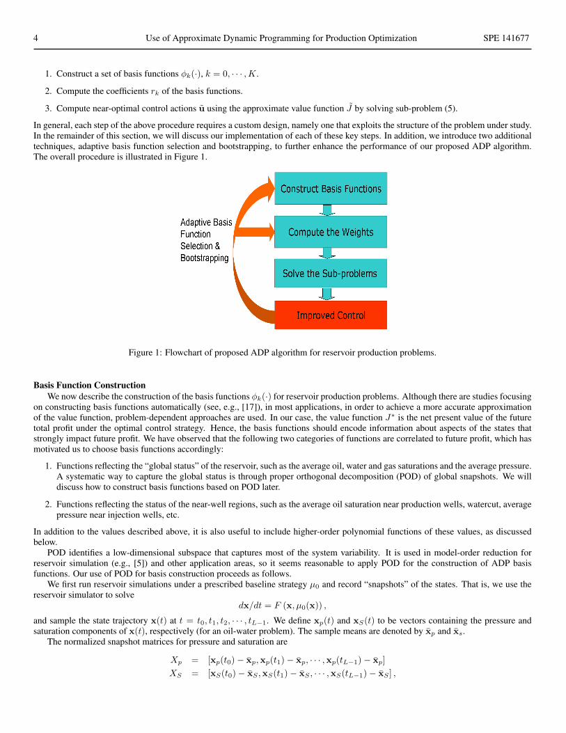
In general, each step of the above procedure requires a custom design, namely one that exploits the structure of the problem under study.In the remainder of this section, we will discuss our implementation of each of these key steps. In addition, we introduce two additionaltechniques, adaptive basis function selection and bootstrapping, to further enhance the performance of our proposed ADP algorithm.The overall procedure is illustrated in Figure 1.

Figure 1: Flowchart of proposed ADP algorithm for reservoir production problems.

Basis Function Construction

We now describe the construction of the basis functions φk(·) for reservoir production problems. Although there are studies focusingon constructing basis functions automatically (see, e.g., [17]), in most applications, in order to achieve a more accurate approximationof the value function, problem-dependent approaches are used. In our case, the value function J∗ is the net present value of the futuretotal profit under the optimal control strategy. Hence, the basis functions should encode information about aspects of the states thatstrongly impact future profit. We have observed that the following two categories of functions are correlated to future profit, which hasmotivated us to choose basis functions accordingly:

1. Functions reflecting the “global status” of the reservoir, such as the average oil, water and gas saturations and the average pressure.A systematic way to capture the global status is through proper orthogonal decomposition (POD) of global snapshots. We willdiscuss how to construct basis functions based on POD later.

2. Functions reflecting the status of the near-well regions, such as the average oil saturation near production wells, watercut, averagepressure near injection wells, etc.

In addition to the values described above, it is also useful to include higher-order polynomial functions of these values, as discussedbelow.

POD identifies a low-dimensional subspace that captures most of the system variability. It is used in model-order reduction forreservoir simulation (e.g., [5]) and other application areas, so it seems reasonable to apply POD for the construction of ADP basisfunctions. Our use of POD for basis construction proceeds as follows.

We first run reservoir simulations under a prescribed baseline strategy µ0 and record “snapshots” of the states. That is, we use thereservoir simulator to solve

dx/dt = F (x, µ0(x)) ,

and sample the state trajectory x(t) at t = t0, t1, t2, · · · , tL−1. We define xp(t) and xS(t) to be vectors containing the pressure andsaturation components of x(t), respectively (for an oil-water problem). The sample means are denoted by xp and xs.

The normalized snapshot matrices for pressure and saturation are

Xp = [xp(t0)− xp,xp(t1)− xp, · · · ,xp(tL−1)− xp]

XS = [xS(t0)− xS ,xS(t1)− xS , · · · ,xS(tL−1)− xS ] ,


respectively. The subspace can now be characterized using singular value decomposition (SVD). Specifically, after applying SVD, wedecompose Xp and XS as Xp = UpΣpV

Tp and XS = USΣSV

TS , respectively, where Σp and ΣS are diagonal matrices made up of

singular values in descending order. Let Up(1 : Np) and US(1 : NS) denote the first Np and NS columns of Up and US , respectively.We define the projection matrix Φ as

Φ =

�Up(1 : Np) 0

0 US(1 : NS)

�. (9)

Note that span(Φ) is a subspace that captures most of the variation in pressure and saturation.Now, we construct basis functions that are polynomials defined on span(Φ). Specifically, letting ϕi denote the ith column of Φ, the

basis functions take the form

φk(x) = Mk

I�

i=1

�ϕTkix�mi

,

where mi are nonnegative integers, Mk is a normalization constant and I is the number of terms in the basis function φk. We say φk isa one-term polynomial if I = 1.

This approach is based on the assumption that the reservoir dynamics under the baseline strategy µ0 are sufficiently similar to thoseunder the optimal strategy µ∗. This is not always the case. One way to address this issue involves bootstrapping, as we will describelater.

It is evident that we can potentially construct many (polynomial) functions reflecting either the status of the entire reservoir or thestatus of near-well regions. Thus, there are many candidate basis functions. However, the use of too many basis functions can resultin onerous computational requirements or performance loss due to overfitting. Thus, in practice, only a subset of all of these candidatebasis functions are used to approximate the value function. We will later propose an adaptive basis function selection scheme, whichchooses an effective subset of basis functions.

Finally, no matter how we construct and choose basis functions, we always include a constant basis function φ0(x) = 1 to achievebetter approximation results and numerical stability. We also normalize all basis functions such that |φk(x0)| = 1 for k = 0, · · · ,K,where x0 is the initial state.

Computation of Coefficients

As discussed above, for a given set of basis functions, we need to compute coefficients to approximate the value function. A numberof ADP algorithms have been proposed for this purpose. Examples include approximate value iteration, approximate policy iteration,temporal-difference learning, Bellman error minimization and approximate linear programming (ALP) (see [3, 25, 19]). In this paper,we use smoothed reduced linear programming (SRLP) with L1 regularization. This is a variant of ALP proposed in [9]. Compared withother ADP algorithms, the main advantage of this procedure (in our context) is that it provides “optimal” solutions in much less timethan alternative approaches. In the remainder of this section, we describe the SRLP algorithm with L1 regularization. A key aspect ofthis algorithm – constraint sampling – is discussed in the Appendix.

Theoretically, the value function can be obtained by solving the infinite dimensional LP (7). However, this is not feasible becausethere are an infinite number of decision variables and an infinite number of constraints. This technical difficulty can be addressed byconstraining the function to the span of the basis functions. In particular, we consider solving

minr

� K�

k=0

rkφk(x)π(dx) (10)

s.t. L(x,u) + F (x,u)TK�

k=0

rk∇φk(x)− αK�

k=0

rkφk(x) ≤ 0 ∀x,u such that S(x,u) ≤ 0,

which is known as the approximate linear program (ALP). However, there are still an infinite number of constraints in the ALP (10),so it cannot be solved exactly. We overcome this issue through constraint sampling; that is, only M, a finite set of sampled statesand control actions, is used to constrain variables. This results in what is known as the reduced linear program (RLP). Let M =�(x(1),u(1)), · · · , (x(M),u(M))

�, where M is the cardinality of M. The RLP takes the form

minr

1

M

M�

m=1

K�

k=0

rkφk(x(m)) (11)

s.t. L(x(m),u(m)) + F (x(m)

,u(m))TK�

k=0

rk∇φk(x(m))− α

K�

k=0

rkφk(x(m)) ≤ 0 ∀m = 1, · · · ,M.

The way in which constraints are sampled significantly impacts the performance of the resulting approximation, and our approach toconstraint sampling is nontrivial. Roughly speaking, we sample the state/action pairs based on a randomized baseline strategy and then


bootstrap this process. Details are provided in the Appendix. We choose the number of sampled states M to be 40 to 60 times the sizeof K, the number of basis functions. It has been observed in some studies [9] that RLP (11) might be in some sense over-constrained.We have also observed that the L1 regularization of r can improve performance. These observations motivate the smoothed reducedlinear program (SRLP) [9] with L1 regularization:

minr,s

1

M

M�

m=1

K�

k=0

rkφk(x(m)) + �||r||1

s.t. L(x(m),u(m)) + F (x(m)

,u(m))TK�

k=0

rk∇φk(x(m))− α

K�

k=0

rkφk(x(m)) ≤ s

(m) ∀m = 1, · · · ,M.

s(m) ≥ 0 ∀m = 1, · · · ,M. (12)M�

m=1

s(m) ≤ θ,

where s =�s(1), s(2), · · · , s(M)

�. There are two parameters to be specified in (12), θ and �. The variable θ ≥ 0 characterizes the extent

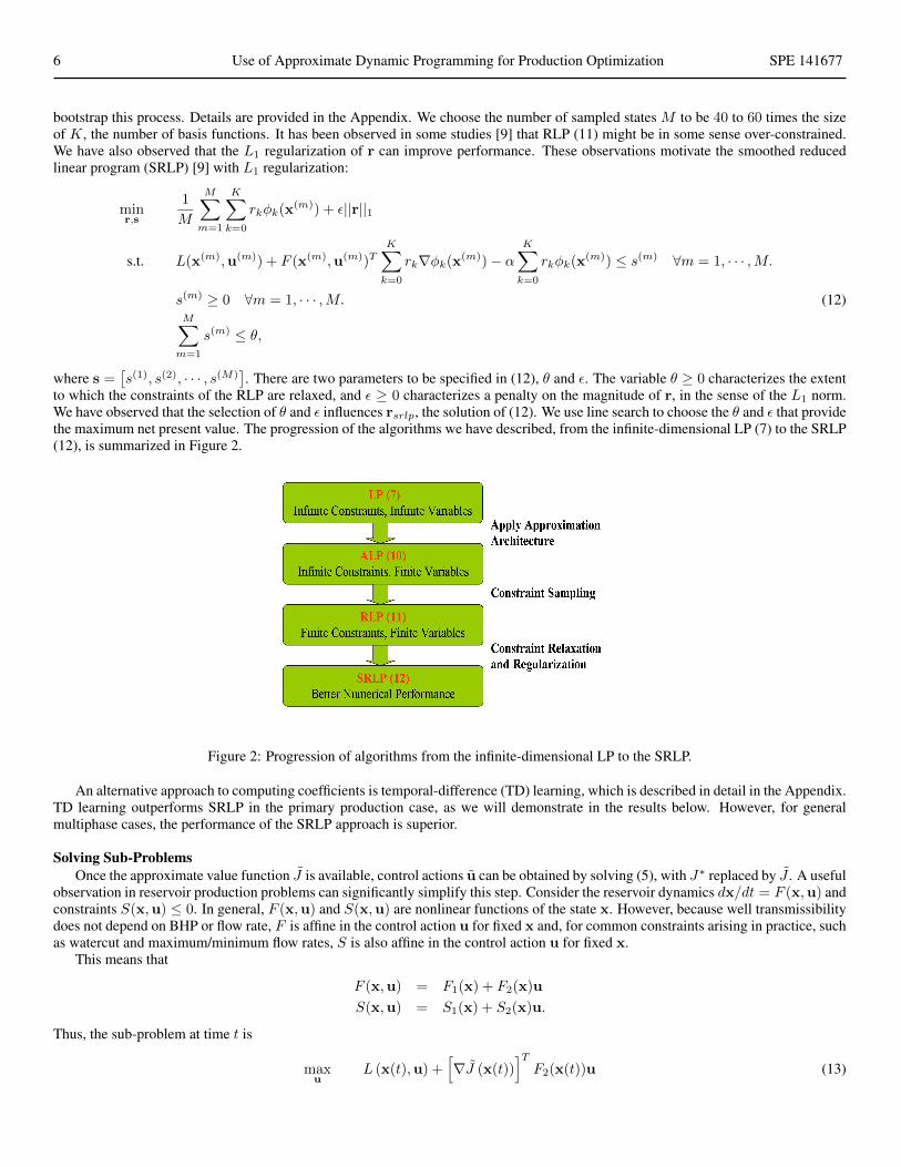
to which the constraints of the RLP are relaxed, and � ≥ 0 characterizes a penalty on the magnitude of r, in the sense of the L1 norm.We have observed that the selection of θ and � influences rsrlp, the solution of (12). We use line search to choose the θ and � that providethe maximum net present value. The progression of the algorithms we have described, from the infinite-dimensional LP (7) to the SRLP(12), is summarized in Figure 2.

Figure 2: Progression of algorithms from the infinite-dimensional LP to the SRLP.

An alternative approach to computing coefficients is temporal-difference (TD) learning, which is described in detail in the Appendix.TD learning outperforms SRLP in the primary production case, as we will demonstrate in the results below. However, for generalmultiphase cases, the performance of the SRLP approach is superior.

Solving Sub-Problems

Once the approximate value function J is available, control actions u can be obtained by solving (5), with J∗ replaced by J . A usefulobservation in reservoir production problems can significantly simplify this step. Consider the reservoir dynamics dx/dt = F (x,u) andconstraints S(x,u) ≤ 0. In general, F (x,u) and S(x,u) are nonlinear functions of the state x. However, because well transmissibilitydoes not depend on BHP or flow rate, F is affine in the control action u for fixed x and, for common constraints arising in practice, suchas watercut and maximum/minimum flow rates, S is also affine in the control action u for fixed x.

This means that

F (x,u) = F1(x) + F2(x)u

S(x,u) = S1(x) + S2(x)u.

Thus, the sub-problem at time t is

maxu

L (x(t),u) +�∇J (x(t))

�TF2(x(t))u (13)


Figure 3: Architecture of the overall ADP algorithm.

s.t. S1(x(t)) + S2(x(t))u ≤ 0.

This problem (13) is easy to solve if the instantaneous payoff function L is concave in u. For example, with the instantaneous payofffunction L defined in (2), the sub-problem at each time reduces to a low-dimensional linear program.

Adaptive Basis Function Selection and Bootstrapping

The ADP algorithm described thus far is “open-loop” in the sense that once a new control u is available, it does not get used to furtherimprove the result. In this subsection, we introduce two advanced techniques, adaptive basis function selection and bootstrapping, to“close the loop” and enhance the performance of the ADP algorithm.

Adaptive Basis Function Selection As discussed earlier, in practical implementations, we need to select a subset of basis functionsfrom the large set of candidates. One way to effectively choose basis functions is through use of adaptive basis function selection.Specifically, we initialize the set of basis functions F as a set containing only the constant basis function φ0(·) = 1. At each iteration,we choose a new basis function and add it to F . Our rule in selecting the new basis function is that, compared to other candidatebasis functions, including the new basis function in F results in the largest increase in the net present value. We continue to add basisfunctions until the addition of any new basis function leads to a decrease in net present value. A detailed description of this algorithm isgiven in the Appendix.

Bootstrapping Another technique to further improve the performance of our ADP algorithm is bootstrapping. Specifically, to con-struct basis functions based on POD and sample the constraints for SRLP (12), we need to sample states and state/action pairs based ona known strategy µ. Theory [8] suggests that, to obtain the best results, we should use an optimal control policy when sampling. Sincean optimal policy is not available (the objective of the ADP algorithm is to find a policy close to optimal), we sample using a baselinestrategy µ0, which inevitably leads to some performance loss.

Bootstrapping has been proposed to address this issue. Specifically, we start from a baseline strategy µ0, then we apply the above-described ADP algorithm to compute an approximate value function J1, which generates a new strategy µ1. Then, we sample statesand state/action pairs based on µ1, and apply the ADP algorithm again to obtain a new approximate value function J2 and a policyµ2. We repeat this procedure until it no longer increases net present value. The Appendix provides a more detailed description of thebootstrapping algorithm.

Figure 3 illustrates the architecture of our ADP algorithm with the incorporation of adaptive basis function selection and bootstrap-ping.


Computational Requirements for the ADP Algorithm

As is the case for other production optimization algorithms, most of the computation in ADP is consumed by the reservoir simula-tions. Thus it is appropriate to assess the computational demands for ADP in terms of the required number of simulations. As shown inFigure 3, the ADP algorithm uses the reservoir simulator to sample states and evaluate the strategy µ. As discussed above, in general,SRLP (12) requires 40K to 60K state samples, where K is the number of basis functions, and each state sample requires one simulation.For example, in Case 2 below, we use 39 basis functions and 2000 state samples. Hence, the number of simulations is 2001, with oneextra simulation for strategy evaluation.

Adaptive basis function selection requires a large number of additional simulations. For this approach, assume there are K candidatebasis functions and we are allowed to use up to Kmax basis functions. One obvious upper bound on the number of required simulationsis 60Kmax+ KKmax. However, this bound is far from tight for the following reasons: first, as is observed in Case 3 below, the numberof basis functions ultimately used (K) tends to be much less than Kmax. Second, the ADP algorithm does not need to reevaluate thestrategy if the computed coefficient of the new basis function is zero, which happens frequently since coefficients are solved by SRLPwith L1 regularization. Thus the number of required simulations in practice is much less than the theoretical bound. For Case 3 below,K = 412, Kmax = 50, so the theoretical bound is around 23600. However, for this case K = 7 and we only perform about 2600simulations.

For the ADP algorithm with bootstrapping, assuming the algorithm applies the bootstrapping B times, the required number ofsimulations will be B times the above results. In practice, it has been observed that the performance tends to degrade after severaliterations of bootstrapping (see [11]; this is also observed in Case 1). Hence, B ≤ 10 in most cases. For Case 1 below, where eachbootstrapping iteration requires 1001 simulations, we observe that the ADP algorithm bootstraps four times and the total number ofsimulations is 4004.

It is evident that ADP run time scales with the number of (candidate) basis functions. In general, the use of more candidate basisfunctions in adaptive basis function selection will improve algorithm performance though it requires more computation. Thus, there isa trade-off between performance and computational effort. It is important to note that both state sampling and adaptive basis functionselection can be implemented in parallel. Thus, by using multiple processors, the elapsed time for the ADP algorithm need not beexcessive.

One way to design the candidate basis function pool is to consider only one-term polynomials. In this case, the number of candidatebasis functions is K = O(Np +NS +Nw), where Nw is the number of wells/well groups and Np and NS are determined during POD.However, in some cases, the “cross terms” (i.e., functions with more than one term) are useful in approximating the value function. Ofcourse, adding all such cross terms will result in an intractably large candidate basis function pool. One way to address this issue is toadd only the cross terms between the first few columns of Φ to the candidate basis function pool. This approach is used in Case 3 below.

We note finally that it is not always necessary to use adaptive basis function selection or bootstrapping. In Case 2 below, for example,useful results are obtained without using either of these procedures.

Simulation Results

In this section, we apply the ADP algorithm to three example cases and compare our results against various baseline strategies.These examples involve single-phase primary production, waterflood with bound constraints, and waterflood with general (nonlinear)constraints. All examples involve two-dimensional reservoir models. In our implementation we use Stanford’s General Purpose Re-search Simulator, GPRS [4, 16] for all simulations and CPLEX, a commercial LP solver, to solve the SRLP (12). Other components ofthe ADP algorithm are implemented in MATLAB.

Case 1: Primary Production with Penalty Term

In the first example, we apply the ADP algorithm to a single-phase primary production case. The reservoir dynamics are describedby a linear flow equation in this case. The geological model is a modified portion of the SPE 10 model (see [6]). The x-directionpermeability field is shown in Figure 4(a). The model contains 35 × 35 grid blocks and has four production wells, each of which iscontrolled by a bounded BHP. We simulate for 6000 days with 200 control periods. The instantaneous profit function is

L(x,u) = revenue from producing oil + λ4�

i=1

log(ui − LBi),

where ui is the BHP for producer i and LBi is its lower bound. The logarithm term penalizes BHPs that are close to the lowerbound. Including this term (in this form) enables an analytical solution of the global optimum using DP. The parameters for Case 1 aresummarized in Table 1.

We apply the ADP algorithm with fixed basis functions and bootstrapping. The basis functions are constructed based on POD.Specifically, POD characterizes a subspace of dimension 13 that captures more than 99.9999% of the variation in pressure (in the senseof singular values). We choose basis functions as one-term polynomials in that subspace. In each iteration of bootstrapping, we resample1000 states to reconstruct the basis functions and better constrain the SRLP (12). Hence, for this case, the ADP algorithm requires 4004simulations in total. Bootstrapping is terminated at the fourth iteration since at this point performance starts to degrade.


(a) Case 1 (b) Case 2

(c) Case 3

Figure 4: Geological model and well configurations for the three cases. Injection and production wells are represented as white crossesand white circles, respectively. Grid blocks are colored to indicate value of permeability in x-direction (red and blue indicate high andlow permeability, respectively).


Table 1: Parameters for Case 1

BHP range for Producer 1 2500-5000 psi BHP range for Producer 2 2400-5000 psiBHP range for Producer 3 2700-5000 psi BHP range for Producer 4 2600-5000 psi

Initial pressure 4500 psi Oil price $42.93/STBLogarithm penalty coefficient λ 1× 104 Discount rate α 5× 10−4

The result using the ADP algorithm is presented in Figure 5(a), where the normalization is with respect to the global optimum. Weobserve that the result from the ADP algorithm is within 2% of the global optimum. The “myopic policy” in Figure 5(a) is a policy thataims at maximizing the instantaneous profit at each time. It is evident that the result of the ADP algorithm is significantly better thanthat using the myopic policy.

(a) SRLP (b) TD Learning

Figure 5: Performance of ADP for primary production problem using (a) SRLP and (b) TD learning.

For this case, the use of TD learning to compute coefficients yields slightly better performance. This is illustrated in Figure 5(b),where the ADP optimum is now within 1% of the global optimum. Each iteration of TD learning requires only one simulation, so 1000total simulations are performed. We have observed, however, that the use of SRLP to compute the coefficients tends to outperform TDlearning for multiphase models.

Although this case is quite simple, it represents one of the few cases where the global optimum can be obtained analytically. Itis significant that, for a case where the global optimum is known, ADP does indeed provide a result that is very close to the globaloptimum.

Case 2: Water Injection with Bounded BHPs

In the second example, we apply the ADP algorithm to an oil-water model with bounded BHPs. The reservoir model contains40 × 40 blocks, with four producers and four injectors. The model is simulated for 3000 days and there are 10 control periods. Thepermeability field in the x-direction is shown in Figure 4(b). The instantaneous profit in this case is computed using (2). The parametersused for Case 2 are summarized in Table 2.


BHP range for producers 2500-4500 psi BHP range for injectors 6000-9000 psiInitial pressure 5080 psi Initial Sw 0.15

Oil price $80/STB Water production cost $36/STBWater injection cost $18/STB Discount rate α 1× 10−3

In this case, we compare the performance of our proposed ADP algorithm with that of the gradient-based method described in [20].


The performance of the gradient-based method depends on the starting point. For this case, we ran the gradient-based method from 200randomly generated starting points and thus obtained 200 local optima. We recorded the best and the worst of these local optimum.

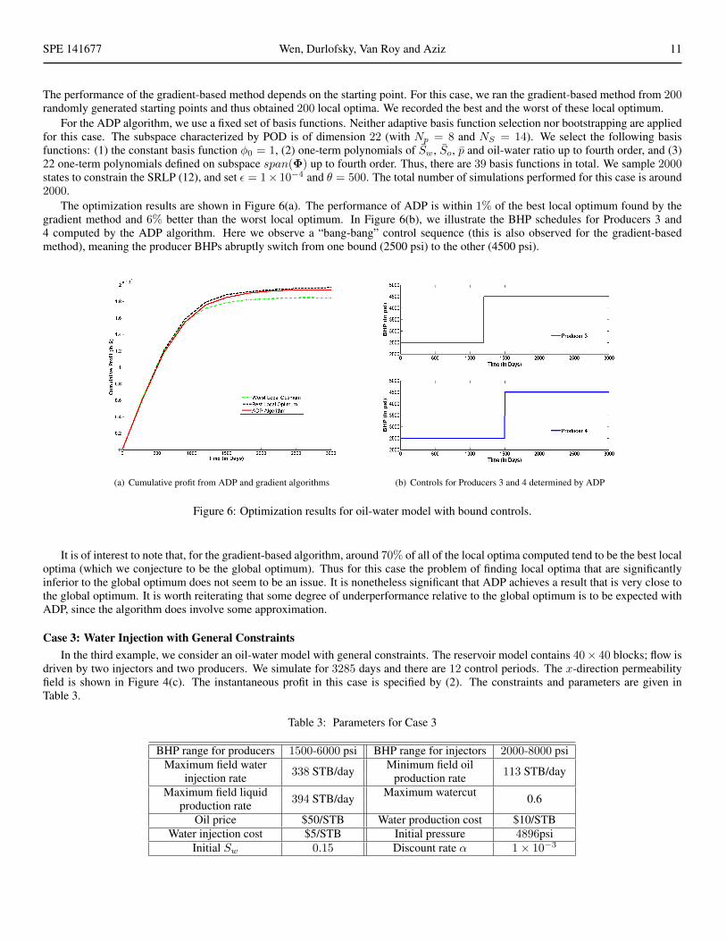
For the ADP algorithm, we use a fixed set of basis functions. Neither adaptive basis function selection nor bootstrapping are appliedfor this case. The subspace characterized by POD is of dimension 22 (with Np = 8 and NS = 14). We select the following basisfunctions: (1) the constant basis function φ0 = 1, (2) one-term polynomials of Sw, So, p and oil-water ratio up to fourth order, and (3)22 one-term polynomials defined on subspace span(Φ) up to fourth order. Thus, there are 39 basis functions in total. We sample 2000states to constrain the SRLP (12), and set � = 1× 10−4 and θ = 500. The total number of simulations performed for this case is around2000.

The optimization results are shown in Figure 6(a). The performance of ADP is within 1% of the best local optimum found by thegradient method and 6% better than the worst local optimum. In Figure 6(b), we illustrate the BHP schedules for Producers 3 and4 computed by the ADP algorithm. Here we observe a “bang-bang” control sequence (this is also observed for the gradient-basedmethod), meaning the producer BHPs abruptly switch from one bound (2500 psi) to the other (4500 psi).

(a) Cumulative profit from ADP and gradient algorithms (b) Controls for Producers 3 and 4 determined by ADP

Figure 6: Optimization results for oil-water model with bound controls.

It is of interest to note that, for the gradient-based algorithm, around 70% of all of the local optima computed tend to be the best localoptima (which we conjecture to be the global optimum). Thus for this case the problem of finding local optima that are significantlyinferior to the global optimum does not seem to be an issue. It is nonetheless significant that ADP achieves a result that is very close tothe global optimum. It is worth reiterating that some degree of underperformance relative to the global optimum is to be expected withADP, since the algorithm does involve some approximation.

Case 3: Water Injection with General Constraints

In the third example, we consider an oil-water model with general constraints. The reservoir model contains 40× 40 blocks; flow isdriven by two injectors and two producers. We simulate for 3285 days and there are 12 control periods. The x-direction permeabilityfield is shown in Figure 4(c). The instantaneous profit in this case is specified by (2). The constraints and parameters are given inTable 3.


BHP range for producers 1500-6000 psi BHP range for injectors 2000-8000 psiMaximum field water

338 STB/day Minimum field oil113 STB/dayinjection rate production rate

Maximum field liquid394 STB/day Maximum watercut 0.6production rate

Oil price $50/STB Water production cost $10/STBWater injection cost $5/STB Initial pressure 4896psi

Initial Sw 0.15 Discount rate α 1× 10−3


For reservoir production problems with general constraints, it can be difficult to find a feasible control strategy without applying anoptimization technique. However, for the sub-problems (13), feasible control strategies can be found as follows. We randomly sampleparameters g and replace the unknown linear function L (x(t),u) + [∇J∗ (x(t))]T F2(x(t))u by gTu. At time t with state x(t), wethen solve the following LP to obtain a feasible control at time t:

maxu

gTu (14)

s.t. S1(x(t)) + S2(x(t))u ≤ 0.

If (14) is infeasible at time t, we restart this procedure from time 0. We use this approach to generate 100 feasible control strategies, andchoose the best one as the baseline for Case 3.

Adaptive basis function selection is used for this case. The coefficients are computed based on SRLP (12). Specifically, we partitionΦ = [Φ1,Φ2], where Φ1 includes the first seven left singular vectors. The candidate basis function pool includes (1) a constant basisfunction φ0 = 1, (2) one-term polynomials of Sw, So, p and oil-water ratio of the entire reservoir up to third order, (3) one-termpolynomials of the average oil saturations in near-producer regions up to third order, (4) all the polynomials defined on span(Φ1) upto third order, and (5) all the other one-term polynomials defined on span(Φ) up to third order. There are thus a total of K = 412candidate basis functions. We use SRLP (12) to compute the coefficients and set θ = 0 and � = 0.005.

The maximum number of basis functions is prescribed as Kmax = 50, so we sample 2000 states to constrain the SRLP. The adaptivebasis function selection algorithm terminates after having added six basis functions. Due to L1 regularization in SRLP, the total numberof strategy evaluations in the course of adaptive basis function selection is about 600.

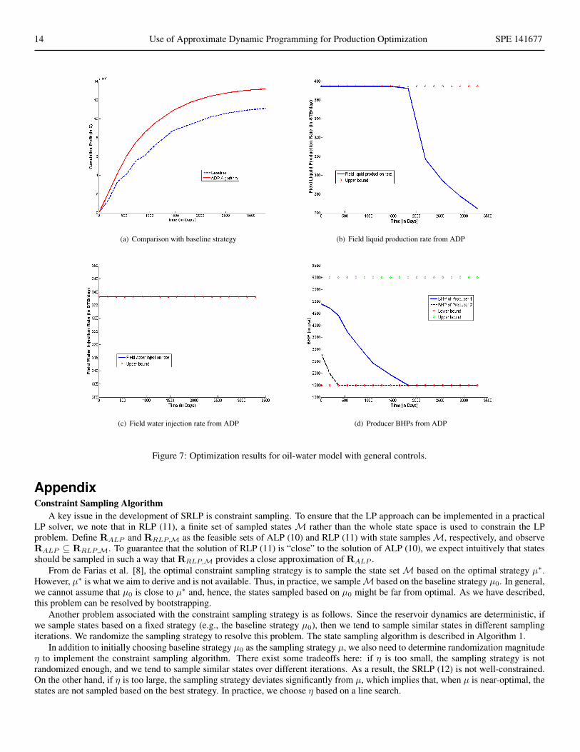
Optimization results are presented in Figure 7(a). The ADP algorithm achieves a 19% improvement compared with the baselinestrategy. We plot the tight constraints over time in Figures 7(b), 7(c) and 7(d). It is evident that the maximum liquid production rate istight at the beginning of simulation, the lower bounds on the producer BHPs are tight at the end of the simulation, and the maximumwater injection rate is tight at all times. The other constraints are not tight over the course of the simulation, which suggests that theycould be relaxed for this example. In any event, this example demonstrates that our ADP algorithm does indeed satisfy bound andnonlinear constraints throughout the simulation.

Concluding Remarks

In this paper, we developed an optimization algorithm for reservoir production based on Approximate Dynamic Programming(ADP). We discussed the general algorithm, described how to construct ADP basis functions, and proposed two additional techniques,adaptive basis function selection and bootstrapping, to enhance algorithm performance. Results were presented for primary productionand waterflooding problems. Both bound constraints and general constraints were considered. Compared with baseline strategies (or inone case results from a gradient-based algorithm), the performance of the ADP algorithm was found to be very good.

In future work, we plan to refine and further test our ADP implementation. This will include testing on larger three-dimensionalproblems and three-phase cases.

Acknowledgements

We are grateful to the industry sponsors of the Stanford Smart Fields Consortium for partial funding of this work. We thank theStanford Center for Computational Earth and Environmental Science for providing distributed computing resources. We also thankDavid Echeverrıa Ciaurri and Huanquan Pan for useful discussions and suggestions.

References

[1] V. Artus, L. J. Durlofsky, J. Onwunalu, and K. Aziz. Optimization of nonconventional wells under uncertainty using statisticalproxies. Computational Geosciences, 10:389–404, 2006.

[2] D. P. Bertsekas. Dynamic Programming and Optimal Control, volume 1. Athena Scientific, 1995.

[3] D. P. Bertsekas and J. N. Tsitsiklis. Neuro-Dynamic Programming. Athena Scientific, 1996.

[4] H. Cao. Development of Techniques for General Purpose Simulators. PhD thesis, Stanford University, 2002.

[5] M. A. Cardoso and L. J. Durlofsky. Use of reduced-order modeling procedures for production optimization. SPE Journal,15(2):426–435, June 2010.

[6] M. A. Christie and M. J. Blunt. Tenth SPE comparative solution project: A comparison of upscaling techniques. SPE ReservoirEvaluation and Engineering, 4:308–317, 2001.

[7] A. S. Cullick, D. Heath, K. Narayanan, J. April, and J. Kelly. Optimizing multiple-field scheduling and production strategy withreduced risk. SPE paper 84239 presented at the 2003 SPE Annual Technical Conference and Exhibition, Denver, Colorado.


[8] D. P. de Farias and B. Van Roy. On constraint sampling in linear programming approach to approximate dynamic programming.Mathematics of Operations Research, 29(3):462–478, August 2004.

[9] V. V. Desai, V. F. Farias, and C. C. Moallemi. The smoothed approximate linear program. In Advances in Neural InformationProcessing Systems 22. MIT Press, 2009.

[10] V. F. Farias and B. Van Roy. An approximate dynamic programming approach to network revenue management. www.

stanford.edu/˜bvr/psfiles/adp-rm.pdf. Working paper.

[11] V. F. Farias and B. Van Roy. Tetris: A study of randomized constraint sampling. In G. Calafiore and F. Dabbene, editors,Probabilistic and Randomized Methods for Design Under Uncertainty. Springer-Verlag, 2006.

[12] J. Han and B. Van Roy. Control of diffusions via linear programming. To appear in Stochastic Programming.

[13] T. J. Harding, N. J. Radcliffe, and P. R. King. Optimization of production strategies using stochastic search methods. SPE paper35518 presented at the 1996 European 3-D Reservoir Modeling Conference, Stavanger, Norway.

[14] M. Haugh, L. Kogan, and Z. Wu. Portfolio optimization with position constraints: an approximate dynamic programming ap-proach. www.columbia.edu/˜mh2078/ADP_Dual_Oct06.pdf. Working paper.

[15] O. J. Isebor. Constrained production optimization with an emphasis on derivative-free methods. Master’s thesis, Stanford Univer-sity, 2009.

[16] Y. Jiang. Techniques for Modeling Complex Reservoirs and Advanced Wells. PhD thesis, Stanford University, 2007.

[17] P. W. Keller, S. Mannor, and D. Precup. Automatic basis function construction for approximate dynamic programming andreinforcement learning. In Proceedings of the 23rd International Conference on Machine Learning, 2006.

[18] F. A. Longstaff and E. S. Schwartz. Valuing American options by simulation: A simple least-square approach. Review of FinancialStudies, 14(1):113–147, 2001.

[19] W. B. Powell. Approximate Dynamic Programming. John Wiley and Sons, 2007.

[20] P. Sarma, L. J. Durlofsky, K. Aziz, and W. H. Chen. Efficient real-time reservoir management using adjoint-based optimal controland model updating. Computational Geosciences, 10:3–36, 2006.

[21] H. P. Simao, A. George, W. B. Powell, T. Gifford, J. Nienow, and J. Day. Approximate dynamic programming captures fleetoperations for schneider national. Interfaces, 40(5):342–352, 2010.

[22] G. J. Tesauro. Temporal difference learning and TD–Gammon. Communications of the ACM, 38:58–68, 1995.

[23] J. N. Tsitsiklis and B. Van Roy. Optimal stopping of Markov processes: Hilbert space theory, approximation algorithms, and anapplication to pricing high-dimensional financial derivatives. IEEE Transactions on Automatic Control, 44(10):1840–1851, 1999.

[24] J. N. Tsitsiklis and B. Van Roy. Regression methods for pricing complex American-style options. IEEE Transactions on NeuralNetworks, 12(4):694–703, July 2001.

[25] B. Van Roy. Neuro-dynamic programming: Overview and recent trends. In E. Feinberg and A. Shwartz, editors, Handbook ofMarkov Decision Processes: Methods and Applications. Kluwer, 2001.

[26] D. Zhang and D. Adelman. Dynamic bid-prices in revenue management. Operations Research, 55(4):647–661, 2007.

[27] D. Zhang and D. Adelman. An approximate dynamic programming approach to network revenue management with customerchoice. Transportation Science, 43:381–394, 2009.


(a) Comparison with baseline strategy (b) Field liquid production rate from ADP

(c) Field water injection rate from ADP (d) Producer BHPs from ADP

Figure 7: Optimization results for oil-water model with general controls.

Appendix

Constraint Sampling Algorithm

A key issue in the development of SRLP is constraint sampling. To ensure that the LP approach can be implemented in a practicalLP solver, we note that in RLP (11), a finite set of sampled states M rather than the whole state space is used to constrain the LPproblem. Define RALP and RRLP,M as the feasible sets of ALP (10) and RLP (11) with state samples M, respectively, and observeRALP ⊆ RRLP,M. To guarantee that the solution of RLP (11) is “close” to the solution of ALP (10), we expect intuitively that statesshould be sampled in such a way that RRLP,M provides a close approximation of RALP .

From de Farias et al. [8], the optimal constraint sampling strategy is to sample the state set M based on the optimal strategy µ∗.However, µ∗ is what we aim to derive and is not available. Thus, in practice, we sample M based on the baseline strategy µ0. In general,we cannot assume that µ0 is close to µ∗ and, hence, the states sampled based on µ0 might be far from optimal. As we have described,this problem can be resolved by bootstrapping.

Another problem associated with the constraint sampling strategy is as follows. Since the reservoir dynamics are deterministic, ifwe sample states based on a fixed strategy (e.g., the baseline strategy µ0), then we tend to sample similar states in different samplingiterations. We randomize the sampling strategy to resolve this problem. The state sampling algorithm is described in Algorithm 1.

In addition to initially choosing baseline strategy µ0 as the sampling strategy µ, we also need to determine randomization magnitudeη to implement the constraint sampling algorithm. There exist some tradeoffs here: if η is too small, the sampling strategy is notrandomized enough, and we tend to sample similar states over different iterations. As a result, the SRLP (12) is not well-constrained.On the other hand, if η is too large, the sampling strategy deviates significantly from µ, which implies that, when µ is near-optimal, thestates are not sampled based on the best strategy. In practice, we choose η based on a line search.


Algorithm 1 Constraint Sampling AlgorithmRequire: Number of samples M , time step ∆, initial state x0, randomization magnitude η and a sampling strategy µ.Ensure: Return a set of sampled state/action pairs M.

for m = 1 to M do

Set initial state x(0) := x0 and set horizon N ∼ Geom�e−α∆

�, where Geom(q) refers to a geometric distribution with parameter

q.for n = 0 to N − 1 do

Set randomized greedy control as u(n∆) = µ (x(n∆)) + ηu, where u is a length(u) dimensional vector whose componentsare i.i.d. uniformly distributed over interval [−1, 1].Set the control as u(n∆) on time interval [n∆, (n+ 1)∆] and run reservoir simulator to obtain x((n+ 1)∆).

end for

Set the mth sample as x(m) = x(N∆) and u(m) = u((N − 1)∆).end for

return M =�x(1),u(1)

�, · · · ,

�x(M),u(M)

�

It is also worth noting that in Algorithm 1, sampling one state/action pair is independent from sampling another. Hence, usingparallel computing, the constraint sampling algorithm 1 can run much faster.

TD-learning Algorithm

An alternative approach for computing the coefficients of the basis functions is temporal-difference (TD) learning. The TD(λ)algorithm for reservoir production problems is summarized in Algorithm 2.

Algorithm 2 TD-learning Algorithm

Require: Set of basis functions {φ0 = 1,φ1, · · · ,φK}, parameters 0 ≤ λ ≤ 1 and γ0, maximum number of iterations I , time step ∆,horizon T , and initial state x0 for reservoir simulation.

Ensure: Return the coefficient vector r.Initialize Zcum = 0, r = 0 and i = 1 {Zcum is the cumulative eligibility vector }for i = 1, 2, · · · , I do

Set Z = 0 and γ = γ0/i.Run a simulation from time 0 to time T , with step size ∆. At each step, generate control greedy to the current approximatevalue function J(x; r) and compute the temporal difference dt = L(x,u)∆ + e−α∆J(xnew; r) − J(x, r) and update Z :=Z+ e−αtdtφ(x).Normalize Z = (1− e−α∆)Z.Update Zcum = λZcum + Z and r := r+ γZcum.Test the performance of J(x; r). If the performance satisfies certain criterion, terminate the loop; otherwise, set i := i+ 1.

end for

return r.

Adaptive Basis Function Selection Algorithm

Adaptive basis function selection algorithm is described in Algorithm 3. In this algorithm, we treat parameters �, η and θ as fixed,though they can be tuned in the SRLP step. Tuning these parameters can potentially improve algorithm performance, though it alsoconsumes more time. Finally, we observe that at each step of Algorithm 3, the adaptive basis function selection iterates over all ofthe candidate basis functions to choose the optimal basis function to add to F , which can be time consuming. However, similar to theconstraint sampling algorithm, parallel computation can significantly accelerate this algorithm.

Bootstrapping Algorithm

The bootstrapping algorithm is described in Algorithm 4.


Algorithm 3 Adaptive Basis Function Selection

Require: Set of sampled states/actions M, set of candidate basis functions {φ0 = 1,φ1, · · · ,φL}, parameters �, η, θ for SRLP, timestep ∆, horizon T and initial state x0 for reservoir simulation.

Ensure: Return a set of basis functions F .Set F = {φ0 = 1}; set evaluated profit J (0) = −∞ and n = 0.repeat

Update n := n+ 1 and set Jr = −∞ and l∗ = −1 {Jr means the best profit of the round.}for l = 1 to L do

if µl /∈ F then

Define F � = F�{φl}.

Selecting F � as the set of basis functions and using parameters �, η and θ, solve SRLP (12) to obtain the coefficients and,hence, the approximate value function J .if the coefficient of φl is not 0 then

Run the reservoir simulator under policy greedy to J , with time step ∆ until time T . Record the profit from the simulationas Je {Je means the evaluated profit.}if Je > Jr

then

Set Jr = Je and l∗ = l.end if

end if

end if

end for

Set J (n) = Jr.if J (n) > J (n−1)

then

F := F�

{µl∗}.end if

until J (n) ≤ J (n−1)

return F .

Algorithm 4 ADP Algorithm with BootstrappingRequire: Baseline strategy µ0.Ensure: Return a near-optimal strategy µ∗∗.

Set k := 0 and J (0) = −∞.repeat

Sample states and state/action pairs based on (randomized) strategy µk. Construct a large set of basis functions based on thesampled states. Set k := k + 1.Apply an ADP algorithm (either with or without adaptive basis function selection) to obtain an approximate value function Jk andits greedy policy µk.Run the reservoir simulation under the strategy µk and record the profit from the simulation as J (k).

until J (k) ≤ J (k−1)

Set µ∗∗ = µk−1.return µ∗∗.

spe 141677 use of approximate dynamic programming for...

Documents