SPE 146776

The Effect of Mechanical Properties Anisotropy in the Generation of Hydraulic Fractures in Organic Shales George A. Waters, Richard E. Lewis and Doug C. Bentley, Schlumberger

Copyright 2011, Society of Petroleum Engineers This paper was prepared for presentation at the SPE Annual Technical Conference and Exhibition held in Denver, Colorado, USA, 30 October–2 November 2011. This paper was selected for presentation by an SPE program committee following review of information contained in an abstract submitted by the author(s). Contents of the paper have not been reviewed by the Society of Petroleum Engineers and are subject to correction by the author(s). The material does not necessar ily reflect any position of the Society of Petroleum Engineers, its officers, or members. Electronic reproduction, distribution, or storage of any part of this paper without the written consent of the Society of Petroleum Engineers is prohi bited. Permission to reproduce in print is restricted to an abstract of not more than 300 words; illustrations may not be copied. The abstract must contain conspicuous acknowledgment of SPE copyright.

Abstract Organic shale reservoirs have very low matrix permeabilities. An extensive conductive hydraulic fracture network is

necessary to impose a pressure drop in the formation to produce hydrocarbons at an economic rate. In addition, horizontal

wells permit the initiation of multiple hydraulic fractures within the reservoir section of the organic shale. The location of the

lateral landing point can have a significant impact on hydraulic fracture geometry.

The stimulated fracture system is influenced by the extensive horizontal laminations that are pervasive in shale reservoirs.

The laminations will strongly influence the hydraulic fracture height because of the difference in rock mechanical properties

measured normal and parallel to the bedding planes. In order to accurately predict fracturing height from logs in this

environment, these mechanical property differences must be taken into account.

A series of sonic logs have been run in organic shales and the stress profile generated from these logs has been estimated,

accounting for the difference in mechanical properties in the vertical and horizontal directions. This stress profile has been

calibrated to measured closure stresses acquired in-situ via micro-fracturing of multiple intervals in vertical, openhole

environments. The results show that ignoring the impact of mechanical property anisotropy can lead to significant errors in

the estimation of hydraulic fracture height. Correspondingly, the optimal landing point of a horizontal wellbore may not be

selected when ignoring this effect. This can result in excessively high fracture initiation pressures, difficulty achieving

injection rate or proppant placement, and unexpected fracture height growth. Simulations of hydraulic fracture width indicate

that thin high-stress intervals can create pinch points that limit vertical fracture conductivity. Each of these factors can result

in un-optimized hydrocarbon productivity.

Mechanical Properties Anisotropy A fundamental property of shale is textural anisotropy due to the platy nature of the abundant clay minerals within its matrix.

As the clay minerals are deposited they are aligned by gravity with the surface of the earth. This fine scale alignment, along

with subtle differences in clay content and other minerals, creates fine-scale layering or laminations. The presence of these

laminations leads to differences, or anisotropy, in many fundamental rock properties including permeability, electrical

resistivity, acoustic velocity, moduli, and Poisson’s ratio. The anisotropic nature of shale should be taken into account when

attempting to predict its behavior. This paper will focus on the effects of anisotropy in organic shale to hydraulic fracturing

and the resulting fracture geometry.

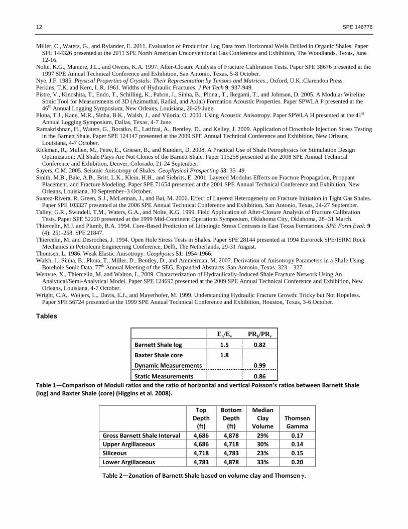
Hornby et al. (1999) demonstrated acoustic anisotropy by comparing compressional slowness recorded in a series of deviated

boreholes drilled in the North Slope of Alaska. They demonstrated that the compressional slowness of shale decreased

significantly as borehole deviation increased. Shale is much slower normal to laminations than parallel to laminations. Sonic

anisotropy was minimal in the underlying sandstone (Fig 1).

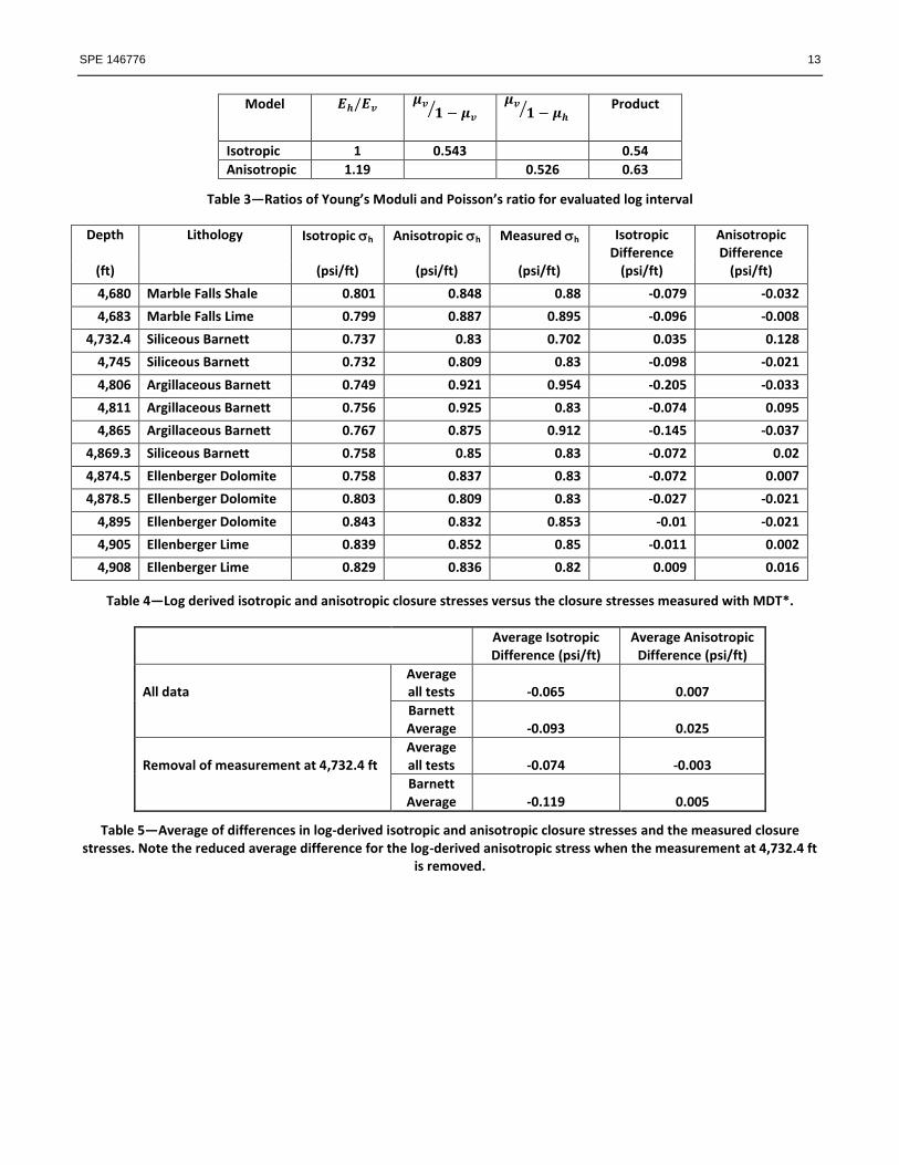
If the shale laminations are horizontal and the formation has no dip, the formation is defined as transverse isotropic with a

vertical axis of symmetry (TIV). The sonic velocities measured in the two vertical orthogonal directions are assumed equal.

They are different from the horizontal velocity measured parallel to the laminations. Fig. 2 demonstrates TIV anisotropy.

Sonic velocity is the same in all directions for an isotropic formation.

2 SPE 146776

Sayers (2005) has demonstrated the relationship between acoustic velocities and elastic moduli for TIV anisotropy through

the application of Hook’s Law shown in Eq. 1. are the elastic stiffness coefficients. A simplified stiffness tensor (Nye

1985; Higgins et al. 2008) that accounts for TIV symmetry is shown in Eq. 2.

................................................................................................................................................... (1)

.................................................................................................................... (2)

C11 represents the horizontally propagating compressional wave, C33 the vertically propagating compressional wave, C44 the

vertically polarized shear wave, and C66 the horizontally polarized shear wave. Each of the Cii is the product of bulk density

and the appropriate velocity squared. C44 is the vertical shear modulus; C66 is the horizontal shear modulus. Higgins et al.

(2008) provide detail in the relationships between these stiffness coefficients, and how they are combined to calculate

Young’s Modulus and Poisson’s ratio for a TIV formation.

Eq. 3 presents the traditional equation used to determine the minimum horizontal stress for an isotropic medium (Thiercelin

and Plumb 1994) that is believed to be linear elastic.

.................................................................................... (3)

Where

= Minimum horizontal stress gradient (psi/ft)

= Poisson’s ratio

= Overburden stress gradient (psi/ft)

= Pore pressure gradient (psi/ft)

= Biot’s elastic constant

= Young’s Modulus (psi)

= Maximum horizontal strain

= Minimum horizontal strain

Variants of this equation are the foundation for calculating stress with acoustic logs. Eq. 4 presents the equation used to

determine the minimum horizontal stress for TIV medium (Thiercelin and Plumb 1994). It will be referred to as the

anisotropic stress equation throughout the remainder of this paper.

................................................................... (4)

Where

= Horizontal Young’s Modulus (psi)

= Vertical Young’s Modulus (psi)

= Horizontal Poisson’s ratio

= Vertical Poisson’s ratio

= Poroelastic constant

The primary difference between Eqs. 3 and 4 is the input of moduli measured in the vertical and horizontal axes

(perpendicular and parallel to shale laminations) in Eq. 4. Both equations will be used to calculate the minimum horizontal

stresses for the example in this paper.

Young’s Modulus is converted from the acoustically measured dynamic value to a static value using a proprietary

approximation for organic shales that is similar, in concept, to published approximations (Lacy 1997; Barree et al. 2009). The

dynamic Poisson’s ratio was not converted. Figs. 3 and 4 present the relationships between static and dynamic core data for a

well in the Baxter Shale (Higgins et al. 2008). These published data present typical core results where there is a well-defined

SPE 146776 3

relationship between the Young’s Moduli, not so with the Poisson’s ratios. The lack of a conversion for Poisson’s ratio does

not prove to be too significant for calculating stress using the anisotropic equation. Using the same core data, the mean

ratio is 1.7. The mean term is 0.30 for static and 0.32 for dynamic data. The difference in the

component of Eq. 4 between using a static or dynamic Poisson’s ratio is 7% of the measurement.

Buller et al, (2010) previously noted the sensitivity of the minimum horizontal stress to the TIV anisotropy via the anisotropic

mechanical property ratios in Eq 4:

. Buller’s work did not quantify the impact of this anisotropy on closure stress, but

instead utilized a series of indexes to qualitatively capture the variation in closure stress with mineralogy. This work follows

on the work of Higgins et al, (2008) and quantifies the closure stress contrast with variations in TIV anisotropy. This allows

the user to perform hydraulic fracturing simulations to determine the impact of parameters such as lateral landing point,

fracturing fluid viscosity and volumes, injection rate and proppant scheduling on created fracture dimensions.

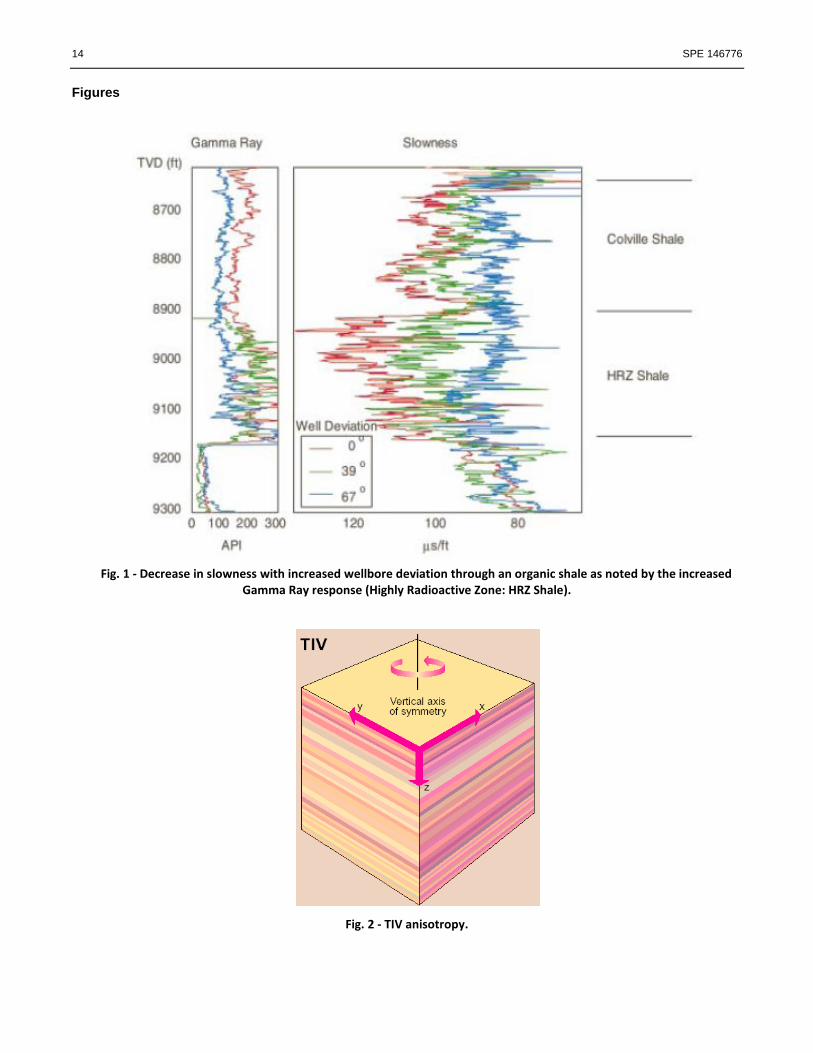
Stress Profile of Heterogeneous Shales Fig. 5 presents both isotropic and anisotropic stress profiles calculated for a well drilled through the Barnett Shale in the Fort

Worth Basin. Log and test data from this well will be the basis for most of the work presented in this paper. These data

include the lower part of the overlying Marble Falls Limestone and the upper part of the underlying Ellenberger Formation.

This well is vertical and formation dip is no greater than 1 degree.

The isotropic stress profile employed vertical compressional and shear slowness measured along the borehole axis. These

measurements are representative of those collected by a conventional dipole sonic log.

The anisotropic stress profile requires both axial and radial slowness measurements in a vertical borehole to account for TIV

anisotropy. Recent advances in acoustic logging permit the estimation of a horizontal shear slowness in a vertical open

borehole through the conversion of monopole Stoneley measurements (Pistre et al. 2005; Walsh et al. 2007). Once the

horizontal shear slowness ( ) is calculated, Eq. 5 can be used to calculate the horizontal compression slowness (Higgins et

al. 2008).

...................................................................................................................................... (5)

Where it is assumed that

Walsh et al. (2007) compared borehole sonic measurements from both vertical and horizontal sonic logs in a pilot well and

associated lateral in the Barnett Shale. Their work confirmed that the horizontal slowness values estimated in the vertical

wellbore were comparable to those measured directly in the lateral wellbore.

Other parameters used in these calculations are:

= 0.443 psi/ft

= 1.1 psi/ft

= 1

= 0

= 0

= 0

Pore pressure was measured at one point in the Barnett Shale (see below), and it was assumed to be constant throughout the

entire interval. Overburden stress was calculated by integrating the density log over true vertical depth and correcting for lack

of surface compaction. Biot’s elastic constant can be measured in the laboratory, but this is very difficult to do in low

permeability rock as it is difficult to change the pore pressure during the tests. The assumption in this paper is that Biot’s

elastic constant is unity. While this may not be the case, it is the authors’ experience that this value, in conjunction with other

calibrated values for pore pressure and tectonic strain, provides an estimate of closure stress in organic shales similar to those

measured through testing.

The magnitude of tectonic strain cannot be directly determined from core or well logs. The Fort Worth Basin presently is in a

relaxed, extensional environment with a low horizontal stress anisotropy (Fisher et al. 2004). Thus, neutral strain values are a

realistic starting point prior to calibrating the calculated stress profile to the measured in-situ values.

4 SPE 146776

Track 5 of Fig. 5 plots and . These two curves overlie in the Ellenberger Formation and in the carbonate rich intervals

within the Marble Falls Limestone. This is expected as these intervals are isotropic. The two diverge, with greater

, throughout almost all of the Barnett Shale interval and in the more clay-rich intervals within the Marble Falls

Limestone. These are intervals with TIV anisotropy, and they coincide with the intervals with elevated clay mineral content

shown in Track 3 of Fig. 5. The clay content and sonic measurements are independent.

Track 9 of Fig. 5 plots the minimum horizontal stress gradient calculated using both an isotropic (Eq. 3) and anisotropic (Eq.

4) model at a scale of 0.6 to 1.1 psi/ft. The two curves overlie in the isotropic Ellenberger Formation and diverge in the

overlying Barnett Shale and the clay-rich parts of the Marble Falls Limestone. The divergence is highlighted with pink fill,

and it coincides with those zones with TIV anisotropy, where is greater than .

There are no core data for this well. Comparison of the log results for the Barnett Shale section of this well to published core

data from the Baxter Shale is presented in Table 1 (Higgins et al. 2008). The comparison between the ratio of horizontal and

vertical Young’s Moduli ratios is comparable with values of 1.5 and 1.8, respectively. Both are reasonable for a TIV shale.

The ratio of horizontal to vertical Poisson’s ratios is 0.82 for the dynamic log measurements. The ratios for the core values

are variable with 0.86 for static and 0.99 for dynamic.

Tracks 10 and 11 of Fig. 5 each present 2D color maps of the calculated minimum horizontal stress gradient for the isotropic

and anisotropic models, respectively. Each track uses a range of colors from red to white to blue to show increasing minimum

horizontal stress from 0.65 to 1.0 psi/ft. The same results are plotted as curves in Track 9.

Shale Mineralogy and Mechanical Properties Mineralogy was determined over the logged interval through a combination of geochemical and triple combo logging strings

(Track 3 of Fig. 5). The penetrated formations were subdivided into volumes of illite, chlorite, smectite, calcite, dolomite,

phosphate, quartz, kerogen, clay bound water, pore water, and gas. Total clay volume for the Barnett Shale has a median of

29%. The Barnett Shale was subdivided into three zones based on clay content (Table 2 and Fig. 5).

The clay content and the stress estimations calculated from sonic logs are independent. Nevertheless, it is apparent that the

TIV zones within this borehole occur where the clay content is elevated or where the clay fraction contains abundant

smectite. The magnitude of TIV anisotropy can be quantified using the Thomsen gamma ( ) parameter (Thomsen 1986)

which is defined in Eq. 6. Gamma is plotted on the right side of Track 5 in Fig. 5.

................................................................................................................................................................. (6)

Fig. 6 is a cross plot between gamma and weight percent clay measured with a geochemical logging tool (Herron and Herron

1996). The correlation between these parameters is a common observation in organic shales indicating the clay content is a

key factor in the development of TIV anisotropy and, ultimately, zones with elevated minimum horizontal stress. The

presence of smectite, as exhibited in the shales within the Marble Falls Limestone, seems to enhance this effect.

If one assumes no horizontal strain and a constant pore pressure, the product of and is the source for

variability in the calculated stress profile. Examination of Eqs. 3 and 4 shows that the primary difference in the calculated

minimum horizontal stress between an isotropic and anisotropic stress profile is driven by rather than .

Table 3 presents values for these two ratios averaged over the evaluated interval. is 19% greater for the anisotropic

model ( is unity for the isotropic model) and the is 3% lower for the anisotropic model. The product of

these ratios for the anisotropic model is 17% greater (0.63 to 0.54). Fig. 7 shows that is related to clay weight percent

within the Barnett Shale for the evaluated well.

Calibration of Sonic-Derived Stress to In-situ Measurements In order to accurately calibrate stress profiles determined from sonic logs, in-situ measurements of closure stress are required.

This has been done successfully in shale reservoirs (Gatens et al. 1990; Thiercelin and Deroches 1994; Ramakrishnan et al.

2009). Closure stress measurements were made in the well in which the sonic derived closure stress is shown in Fig. 5, and

they are plotted on Track 9. The technique utilized to measure these values has been previously described (Ramakrishnan et

al. 2009). This technique uses the Modular Formation Dynamic Tester* (MDT) downhole tool which is capable of inflating

two packers separated by approximately 3 ft, isolating small intervals in an open hole section, and then using a pump within

the tool to initiate a hydraulic fracture. Gauges within the tool monitor the pressure and temperature during the injection and

pressure decline sequence. Interpretation of the pressure responses yield values of fracture initiation pressure, fracture

extension pressure, the source of the pressure decline (matrix or fissure controlled, fracture extension, or height/length

recession) and closure stress. Potentially, pore pressure and transmissibility can be determined from a post-fracture closure

pressure decline analysis.

SPE 146776 5

Closure stress measurements were made in multiple Barnett Shale intervals as well as the underlying Ellenberger Formation

and overlying Marble Falls Limestone. An accurate measure of closure stress in a rock with isotropic mechanical properties

is required to calibrate the sonic derived stress profile. Eqs. 3 and 4 include several parameters that cannot be quantified by

either core or log measurements: pore pressure gradient, Biot’s elastic constant and the horizontal strain coefficients. Pore

pressure can be measured independently (see below). The most reliable way to estimate horizontal strain is to measure the

closure stress in a rock that is most sensitive to strain. Examination of Eqs. 3 and 4 indicate that this is a zone with the highest

Young’s Modulus, typically a carbonate. The Ellenberger Formation is the most appropriate zone through the interval and

was used as the tectonic strain calibration point.

The interval selection methodology has been previously described (Ramakrishnan et al. 2009). Intervals anticipated to have

the lowest closure stress are tested first to minimize the differential pressure placed on the inflatable packers in the testing

tool. Those intervals thought to be most significant in controlling the hydraulic fracture geometry are selected. Small

intervals such as thin carbonates are generally not selected as they are not expected to vertically contain hydraulic fractures.

Identification of these intervals via conventional triple combo logs can be problematic. These intervals are commonly

concretions in organic shales and not considered to be viable hydraulic fracturing barriers. Concretions are readily identified

by borehole resistivity images from an electrical micro-resistivity imager log. Fig. 8 shows the triple-combo log response

through an interval containing concretions. Classic log responses for a carbonate – low gamma ray activity, high resistivity,

low neutron porosity, high bulk density, and high Pe – are evident. The electrical micro-resistivity imager log response over

the same interval is in Fig. 9. The concretions are resistive and appear to be laterally non-continuous. The nature of the

concretions is evidenced by their small size and the deformation of surrounding strata caused by their formation.

Pore pressure is required to calibrate the stress profile, but its estimation in ultra-low permeability shale is problematic

because of the extended shut in period required to monitor pressure declines/inclines. One technique that has the potential to

accurately estimate pore pressure in a timely manner is post-hydraulic fracture closure pressure decline analysis. This method

relies on the pressure transient to develop into pseudo-radial flow (Nolte et al. 1997), although analysis when the transient is

in transition from pseudo-linear flow to pseudo-radial flow can yield accurate values (Talley et al. 1999). For a timely

analysis, hydraulic fractures of short length created at low injection rates are requisite, as the necessary shut in time increases

exponentially with the fracture length (Talley et al. 1999).

There are several competing factors when attempting to perform post-closure pressure decline analyses in ultra-low

permeability shales. As stated, desired fracture half lengths are short. But hydraulic fractures must penetrate through the near-

wellbore stress concentration to escape its influence on the pressure decline. An estimate of the desired injected volume to

achieve this is made a priori based on the following assumptions:

Fluid efficiency during injection = 100%

Fluid Flow Behavior Index (n’) = 0.8

Horizontal Young’s Modulus (Eh) = 3,000,000 psi

Hydraulic Fracture Height (hf) = 4 ft

Anticipated Net Pressure (PN) = 250 psi

Desired Fracture Half Length (xf) = 10 ft

For such a geometry, PKN behavior can be assumed (xf > 2hf). Fracture compliance (Perkins and Kern 1961) for this

geometry (Eq. 7) yields a hydraulic width (wf) of 0.005 in.

.......................................................................................................................................................... (7)

Where

.......................................................................................................................................... (8)

with n’ being the power law flow behavior index.

Beta adjusts the fracture width to account for the change in Net Pressure that occurs immediately after pumping ceases and

friction losses along the fracture face are minimized due to reduced fluid flow within the fracture. We assumed a water based

drilling fluid with a n’ = 1, beta = 0.8. Material balance indicates an injected volume of 0.25 gal of drilling mud is required to

create a fracture that will penetrate beyond the stress concentration of approximately four times the wellbore diameter of 8.75

inches (El Rabaa 1989).

6 SPE 146776

An injection of 0.25 gal following fracture initiation was made in the siliceous Barnett Shale interval at 4,732.4 ft. The

subsequent pressure decline was monitored for 8 hours (Fig. 10). This interval was selected for an extended pressure decline

as the permeability was expected to be moderately high for an organic shale (~ 0.0002 md) based on the log evaluation. The

G Function decline analysis indicated matrix leakoff, or possibly slight fracture height or length recession, and yielded a

closure stress of 3,322 psi (0.702 psi/ft) (Fig. 11). The instantaneous shut in pressure was 3,481 psi yielding a Net Pressure of

159 psi.

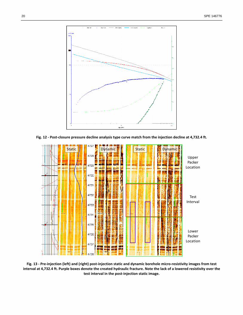
Pressure decline analysis was performed in real time until a reliable value of pore pressure was attained. Fig. 12 shows the

post-closure pressure derivative versus 1/FL2. Reservoir response is represented when the pressure derivative (blue dots) has a

negative slope. In this case the pressure transient is in the transition from pseudo-linear flow to pseudo-radial flow. Type

curves, solid lines in Fig. 12, allow for pore pressure approximation in this case, although the analysis is non-unique.

Therefore, a sensitivity analysis was performed in which reasonable type curve matches were obtained for variable pore

pressures. Lower and upper bounds of pore pressure were determined to be 2,065 psi and 2,100 psi, respectively, a difference

of 0.007 psi/ft. Thus, a pore pressure gradient of 0.443 psi/ft was accurately acquired in an ultra-low permeability organic

shale in a reasonable period of time.

The fact that the G Function superposition indicated matrix leakoff behavior during fracture closure is somewhat perplexing.

This is an indication that fluids can indeed imbibe into rocks with permeability on the order of 0.0002 md. Yet the post-

injection static resistivity image from the electrical imaging log does not portray a lowered “resistivity ring” over the

borehole interval that was exposed to the injection pressure, indicating that no imbibition of drilling fluids occurred at the

wellbore interface during the injection and decline (right side of Fig. 13). In addition, filter cake was not apparent on the

borehole to support the imbibition theory during drilling. A possible explanation is that the drilling process has altered the

pores at the borehole thereby reducing leakoff. Pores exposed to a hydraulic fracture would not have undergone such

alteration. This issue requires further study, but it has been the authors’ observation that a “resistivity ring” has yet to be

identified across intervals in organic shales where stress tests have been performed. Furthermore, pressure dependent leakoff

from the G Function analysis is the norm, not the exception, indicating that fissure leakoff is the dominant pressure decline

mechanism. These observations are based on the testing of more than 200 organic shale intervals using this technique.

As shown in the pre-injection electrical imager log images on the left side of Fig. 13, there is a pre-existing conductive

fracture over this interval. This near-vertical fracture is striking N10W. This interval also exhibited polarization of the shear

waves into fast and slow directions. Track 1 of Fig. 5 shows the relative amount of this anisotropy as a difference in energy

between the waveforms aligned with the fast direction (maximum energy) and those aligned with the slow direction. Note

that this is the only interval within the Barnett Shale that exhibits this type of anisotropy. The direction of the fast shear over

this interval is N9W, basically the same as the fracture orientation measured with the electrical image log. The dominant

mechanism for this anisotropy can be identified through the analysis of dipole dispersion curves (Plona et al. 2000), and Fig.

14 indicates that it is intrinsic. Because the bedding is flat-lying, the source for this anisotropy is a natural fracture. Thus

acoustic dispersion analysis can aid in determining whether conductive fractures identified with borehole imaging tools are

natural or mechanically induced during the drilling process. The induced hydraulic fractures imaged in the post-injection

electrical image log strikes N70E & N90W. The difference in strike of the pre-existing fracture and the hydraulic fracture is a

strong indication that the pre-existing fracture is natural and not induced, and validates the acoustic log analysis. The strike of

the hydraulic fracture is somewhat more easterly than has been noted in the basin (Fisher et al. 2002), but is still consistent

with the structural setting in the basin. Also of interest is the nature of the induced fractures. The wing striking N70E is a

single, vertical fracture. The fractures striking N90W are a series of conjugate, inclined fractures. The pressure response

during the injection does not exhibit classic behavior (Fig. 15). The rapid pressure increases and decreases during injection

may be an indication of propagation of en echelon fractures. The fact that the hydraulic fractures are not offset by 180

degrees indicates that the lowest stress concentrations are not aligned on opposite sides of the borehole. Rock texture or

mechanical properties anisotropy (Suarez-Rivera et al. 2006) are likely influencing this behavior. It is possible that the

existing natural fractures are influencing this behavior as well.

The post-injection electrical image log allows one to quantify the upper bound of hydraulic fracture height and to estimate the

fracture half length. The right side of Fig. 13 shows that the hydraulic fracture height is 4.2 ft. Because subsequent larger

injections to validate closure were performed following the 8 hour shut in, the final imaged fracture height is likely greater

than created during the initial 0.25 gal injection. A Net Pressure of 159 psi was developed during the first injection (Fig. 11).

The average horizontal static Young’s Modulus over the fractured interval, as determined from the sonic log analysis, is 2.89

x 106 psi. The G Function pre-closure decline analysis yields a fluid efficiency of 74% (ct = 0.00002 ft/min

0.5), a fracture

length of 20 ft, and a hydraulic width of 0.0025 in. To honor the hydraulic width of 0.0025 in, a fracture height of 3.1 ft is

required in Eq. 7. This is less than the 4.2 ft imaged by the electrical borehole imager indicating that additional height growth

occurred during the subsequent injections. The corresponding hydraulic fracture half length of 20 ft is well beyond the near-

wellbore stress concentration (El Rabaa 1989).

SPE 146776 7

An alternative G Function decline analysis yields a closure stress of 3,160 psi (0.67 psi/ft) (Fig. 16). The resulting higher Net

Pressure of 321 psi requires either a horizontal Young’s Modulus of approximately 10 x 106 psi or a much more contained

fracture of approximately 1.7 ft. This modulus is unrealistically high. While it is possible that the initial injection only created

a fracture of this height, to do so requires a fracture half length of 37 ft and a large Net Pressure (321 psi) for a very small

injection (0.25 gal). It is the authors’ opinion that a fracture geometry aspect ratio in excess of 40 (2 x 37 ft / 1.7 ft) is

unrealistic for these conditions. In summary, the post injection electrical micro-resistivity image improves the interpretation

of the pressure decline analysis by setting an upper bound on fracture height growth and ultimately leading to a more accurate

value of closure stress. This process was used to determine the closure stress in the 13 intervals that were in-situ stress tested

in the Ellenberger Formation, Barnett Shale, and Marble Falls Limestone for the subject well. These results are plotted in

Track 9 of Fig. 5.

With a measured pore pressure that is assumed to be constant through all intervals, the sonic derived stress profile can now be

estimated and compared to the measured closure stress values. Table 4 displays the sonic-derived isotropic and anisotropic

stress gradients as well as the measured values of stress at each depth where testing was performed. The sonic interpretation

provides a closure stress estimate every 6 in. The log values posted in Table 4 are averaged over a 5 ft interval as this more

accurately represents the interval over which vertical hydraulic fractures grew. Table 5 presents the average of the

differences between both the isotropic and anisotropic log-derived stress gradients and the measured stresses. The average of

the difference for the log-derived anisotropic stress is lower than that for the log-derived isotropic stress. The average

difference for the log-derived anisotropic stress goes almost to zero if the measurement at 4,732.4 ft is removed. This point

does represent an anomalous zone where there is image and sonic evidence for open natural fractures within the Barnett Shale

(Fig 13) as previously discussed. No other tested zones showed any indication of open natural fractures. From the micro-

resistivity image (Fig. 13) it is clear that the injection created a new hydraulic fracture. It is possible that the existing natural

fracture has relieved the local stress to the point that a measurably lower closure stress occurs. Negative strain coefficients are

required to calibrate the sonic derived stress profile in this environment. Sonic dispersion and radial profiling plots with

characteristics like Fig.14 have identified similar behavior in other Barnett Shale wells where MDT measured stresses were

lower than log estimated stresses that did not utilize negative strains. These observations suggest that naturally fractured

intervals could be optimal intervals for landing laterals or placing perforation clusters because they are indicators of a lower

stress and corresponding low fracture initiation pressures.

Multiple conclusions can be drawn from the comparison of measured closure stress with the log derived isotropic and

anisotropic stress profiles:

1. The sonic-derived closure stresses in the Ellenberger Formation for both the isotropic and anisotropic processing

closely match the measured values. This is because the Ellenberger Formation is an isotropically behaving carbonate

with few to no laminations.

2. The sonic stress profile derived from the isotropic equation (Eq. 3) significantly under-predicts the closure stress in

the laminated Barnett Shale and Marble Falls Limestone. At only one depth where closure stress was measured

within these zones is the isotropic stress within 0.07 psi/ft of the measured stress: a naturally fractured interval at

4,732.4 ft.

3. The anisotropic stress profile more accurately matches the measured closure stress values in these laminated shales.

In all but one case the predicted closure stress is within 0.10 psi/ft, and most differ by less than 0.04 psi/ft.

When considering the implications for hydraulic fracture height growth the following conclusions can be made:

1. The isotropic stress profile predicts a large stress contrast across the Barnett Shale – Ellenberger Formation

interface. The measured downhole stress values do not support this.

2. The anisotropic stress profile does indeed predict that there is no significant stress contrast between the lower

Barnett Shale and the underlying Ellenberger Formation.

3. Hydraulic fractures may easily grow into the underlying Ellenberger Formation, especially if initiated in the high

stress, argillaceous lower zone of the Barnett Shale.

4. Downward fracture height growth into the Ellenberger Formation would be unexpected if conventional dipole sonic

stress profiles are employed that do not account for TIV anisotropy.

Stress profiles alone do not accurately predict hydraulic fracture height growth. Inspection of Track 11 of Fig. 5 would

suggest that downward fracture height would be contained by the lower argillaceous zone of the Barnett Shale starting at

4,783 ft, and upward growth contained by the Marble Falls Limestone from 4,624 – 4,662 ft. Hydraulic fracture simulations

are required to accurately predict hydraulic fracture height growth.

Applications for Lateral Landing Point and Hydraulic Fracture Geometry “Horizontal wells” in organic shales is somewhat of a misnomer as the wells are frequently drilled toe up for gravity

drainage. Alternatively, attempts are often made to drill parallel to expected bedding planes to land the lateral in the “sweet

spot.” Because of their highly laminated nature this is extremely difficult to do, especially when a gamma ray measurement is

8 SPE 146776

the primary record used for steering. The end result is that productivity along a lateral can be quite variable (Miller et al.

2011).

Laterals that intersect different strata along their length can have inconsistent hydraulic fracture heights because of their

variable fracture initiation pressures. Hydraulic fracture simulations should be performed to quantify this behavior. Vertical

fracture height growth in shales with TIV anisotropy is not solely a function of the minimum horizontal stress contrast

between the various layers. The variability in the mechanical properties between adjacent laminations may impact vertical

fracture height growth (Wright et al. 1999; Smith et al. 2001), a situation akin to the influence of vertical natural fractures to

lateral fracture complexity. This will have the effect of limiting fracture height growth. Conventional hydraulic fracture

simulators cannot model this behavior, although more advanced fracturing simulators can begin to address complex fracture

systems developed in fissured media (Wenyue 2009; Meyer 2011). But simulators can be used to get an order of magnitude

estimate of fracture height growth and how this varies with initiation point.

A limitation of most hydraulic fracturing simulators is that they do not model complex vertical fractures of variable azimuths.

Organic shales can be a highly fractured media and exhibit this behavior. To approximate the impact of this complexity on

hydraulic fracture height growth one may use empirically derived leakoff coefficients to model “leakoff” into natural

fractures. The total leakoff coefficient (Ct) can be determined via simulation iterations to match the height, length, and Net

Pressure build of the dominant planar fracture generated. Microseismic monitoring is used as the reference of the fracture’s

length and height. Such a calibrated fracturing simulator can then be used with some accuracy to estimate height growth. The

process can certainly indicate when variable fracture heights are created because of differing fracture initiation/lateral landing

points.

A series of hydraulic fracture simulations employing a fully 3D, finite difference, planar simulator was performed to evaluate

the effect of lateral landing point on hydraulic fracture geometry. The calibrated anisotropic stress profile was used and the

results compared to those modeled using the incorrect conventional isotropic stress profile. Simulations were performed at

four depths as noted in Fig. 5.

Fig. 17 shows the pump schedule used in the simulations. This schedule is based on the assumptions that there are three

perforation clusters per frac stage, and symmetric hydraulic fractures are propagating from each perforation cluster. This

equates to a 100 bpm pump rate with 495,000 gal of Slickwater and 290,000 lbm of 40/70 mesh sand per stage. This schedule

is comparable to what is pumped on horizontal wells in the Barnett Shale. No interaction between the simultaneously

propagating fractures is modeled. The Stage Name column in Fig. 17 portrays a typical proppant schedule. The Prop Conc.

column shows that no proppant was actually included in the simulations. This was done so an upper bound on hydraulic

fracture dimensions could be established. Modeled proppant transport with Slickwater fracturing fluids will result in the

lower perimeter of the hydraulic fracture screening out. This may result in an underestimation of fracture height growth.

Therefore, proppant was excluded from these simulations.

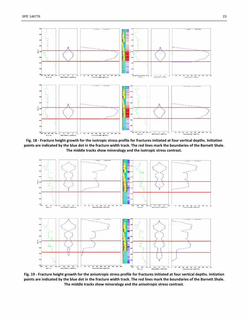
The geometries for these simulations with the isotropic profiles are shown in Fig. 18. The anisotropic geometries are shown

in Fig. 19. The red horizontal lines on each fracture geometry figure denote the boundaries for the Barnett Shale.

Isotropic Stress Profile Fracture Geometries Because of the high stresses predicted by the isotropic stress profile in the underlying Ellenberger Formation and overlying

argillaceous interval of the Marble Falls Limestone, the simulated hydraulic fractures are well contained within the Barnett

shale. According to the model, there is only minimal growth into the Marble Falls Limestone and no growth into the

underlying Ellenberger Formation. This is true for all four simulations and indicates that lateral landing point does not play a

significant role in the height and length of hydraulic fractures provided that an isotropic model is representative of the Barnett

Shale.

Anisotropic Stress Profile Fracture Geometries The fracture geometries are much different when the calibrated anisotropic stress profile is used in the simulations. In all

cases significant upward height growth through the Marble Falls Limestone is predicted. A large percentage of the fracturing

fluid is placed in the Marble Falls Limestone rendering the Barnett Shale less efficiently stimulated.

The extent of the downward growth is a function of the fracture initiation point. When the perforations are placed within the

upper argillaceous zone of the Barnett Shale (Table 2), the lower argillaceous zone of the Barnett Shale performs as a barrier

to downward fracture growth into the Ellenberger Formation. In this case the Barnett Shale is not completely contacted by the

stimulation treatment. Any hydrocarbons below approximately 4,780 ft would probably not be produced due to lack of

stimulation. Over this bottom section of the Barnett Shale there is an estimated total Gas in Place (GIP) of 24 BCF/mi2 (Track

4 of Fig. 5). This represents 48% of the total GIP of 50 BCF/mi2 through the entire Barnett Shale interval that is not

effectively stimulated.

SPE 146776 9

For the two simulations in which the fracture is initiated in the bottom argillaceous zone of the Barnett Shale (Table 2), the

downward growth of the fracture extends into the Ellenberger Formation. This is because the fracture is initiated in a high

stress interval that is bounded by lower stress intervals. In these cases the bottom of the Barnett Shale does receive some

stimulation, although the hydraulic fracture lengths are minimal. More relevantly, these stimulation treatments may contact

producible formation water that is common to the Ellenberger Formation. Because of its much larger mobility, water in the

Ellenberger Formation will be produced preferentially to gas in the Barnett Shale.

Another potential issue with landing the lateral in a high stress interval is the narrow hydraulic fractures that are created near

the borehole in these intervals. The two simulations with fractures initiated in the lower argillaceous Barnett Shale intervals

both exhibit these pinch points at the depth of the perforations (Fig. 19). These width restrictions may cause significant issues

with proppant placement. Treatments initiated from these intervals may also exhibit significant near-wellbore pressure losses

during injection that may limit pump rate because of high treating pressures. Lastly, these argillaceous intervals not only

posses a high stress, they normally have low horizontal Young’s Moduli, which may lead to proppant embedment and

corresponding fracture conductivity impairment that can adversely affect productivity (Miller et al. 2011).

The fracture geometry simulations yield several conclusions:

1. The calibrated anisotropic stress profile shows that significant upward fracture growth through the Marble Falls

Limestone occurs in all simulations, independent of the fracture initiation point.

2. The basal 80 ft of the Barnett Shale is not stimulated unless the fracture is initiated within this interval. In all cases

this argillaceous Barnett Shale is rendered inefficiently stimulated.

3. For fractures initiated in the high stressed, lower argillaceous zone of the Barnett Shale downward fracture growth

into the Ellenberger Formation is predicted. As the Ellenberger Formation is frequently wet, fractures initiated in

these lower zones run the risk of producing native water.

4. Simulations using the uncalibrated isotropic sonic-derived stress profile grossly under predict hydraulic fracture

height.

5. The fracture height is insensitive to fracture initiation point for simulations using the uncalibrated sonic-derived

isotropic stress profile.

6. Growth into the underlying Ellenberger Formation, with the potential for water production, is not predicted with the

isotropic stress profile. Simulations using such profiles may provide a false sense of security that the well will

produce free of formation water.

7. Variable lateral landing points create variable fracture geometries when using the calibrated anisotropic stress

profile.

8. Fractures initiated in the lower argillaceous Barnett Shale interval may experience high treating pressures, and

placing proppant may be problematic. This is because of the pinch points associated with initiating fractures in these

high stressed, low Young’s Modulus intervals.

9. Fracture conductivity may constrain production for laterals landed in the lower argillaceous Barnett Shale interval.

Comparison to Alternative Interpretation Techniques One technique that is used to select lateral points and perforation location is to compare the vertical Young’s Moduli and

vertical Poisson’s ratios derived from dipole sonic logs. Those zones with the highest vertical Young’s Modulus and lowest

vertical Poisson’s ratio are defined as brittle. The Brittleness Index (BI) (Grieser and Bray 2007; Rickman et al. 2008) is

defined in Eq. 9. It was calculated for the Barnett Shale well using the vertical Young’s Moduli and vertical Poisson’s ratios

from the Marble Falls Limestone, through the Barnett Shale, and into the Ellenberger Formation.

–

.............................................................................................................. (9)

Where

= Minimum vertical Young’s Modulus in interval of interest (psi)

= Maximum vertical Young’s Modulus in interval of interest (psi)

= Minimum vertical Poisson’s ratio in interval of interest (psi)

= Maximum vertical Poisson’s ratio in interval of interest (psi)

The resulting value is an index scaled from 0 to 100. It is plotted with the isotropic and anisotropic stress profiles computed

from the sonic log in Track 9 of Fig. 5. It is also plotted as a 2D color map in Track 12 of Fig. 5. With proper scaling of the

index there is good agreement between BI and the isotropic stress profile. This can also be seen in the crossplot of Fig. 20.

This should be expected as this stress profile is driven by lithostatic loading via the vertical Poisson’s ratio used in the BI

calculation (Eqs. 3 and 9). Poisson’s ratio is essentially a proxy for minimum horizontal stress for the BI. However, the sonic-

10 SPE 146776

derived stress profile that matches the measured in-situ closure stresses is not a function of lithostatic loading only. It is much

more sensitive to the difference in the vertical and horizontal Young’s Moduli (Eq. 4). Consequently, there is much less

agreement between BI and the calibrated anisotropic stress profile (Fig. 21). The error associated with using a lithostatic

model in this way can be significant. The anisotropic stress model based on the sonic log predicts a high stress in the lower

argillaceous zone of the Barnett Shale, and the in-situ stress measurements confirm this (Table 4). Yet the lowest BI through

the whole section of the wellbore is in this interval (Track 9 of Fig. 5). If BI is used land a lateral in this lower interval then

the risk of fracturing into the Ellenberger Formation is greatly increased (Fig. 19). Stimulation placement and fracture

conductivity may be compromised as well.

As previously demonstrated, the stress profile and corresponding fracture height growth in a laminated reservoir is a function

of the mechanical properties anisotropy as outlined in Eq. 4 and noted by Buller et al. (2010). These properties therefore

provide an indication of expected hydraulic fracture height growth. For given values of overburden, pore pressure and

tectonic strains closure stress is directly proportional to these mechanical properties. Eq. 10 shows this proportionality.

................................................................................................................................................. (10)

Plotting this Shale Stress Index (SSI) versus depth will therefore provide an indication of the expected closure stress contrast

through the interval without inputs for pore pressure and horizontal strains. Track 8 of Fig. 5 compares the SSI to the BI.

Comparison to the adjoining Track 9 shows the SSI to effectively mimic the calibrated anisotropic stress profile. The BI does

not because it is based on a lithostatic loaded stress model. Therefore, the SSI can be used as an indicator of closure stress in

shales without having to quantify the overburden, pore pressure or strain coefficients as long as these parameters do not vary

significantly through the intervals. Fig. 22 plots the SSI vs. the anisotropic stress profile. As expected the plot is a straight

line as defined by Eq. 4. The slope is and its y-intercept is plus any horizontal strain components.

The SSI can be used to reliably select lateral landing points from pilot hole logs. From Track 8 of Fig. 5 the optimum lateral

landing point based on the SSI is from 4,720 ft to 4,755 ft. This is at least 121 ft from the Ellenberger Formation. The

anisotropic stress profile in Track 9 of Fig. 5 shows this to be the lowest stressed interval within the Barnett Shale. Fracture

simulations (Fig. 19) show that hydraulic fractures initiated in this interval do not penetrate the Ellenberger Formation.

Contrast this to the interval from 4,794 ft to 4,816 ft with the lowest BI. The anisotropic stress profile shows that this is

actually the highest stressed Barnett Shale interval. This zone is also only 60 ft from the Ellenberger Formation and fracture

simulations (Fig. 19) show that fractures initiated in this interval will grow into the Ellenberger Formation.

Conclusions 1. Shale reservoirs are laminated and, assuming flat-lying dip, these laminations create TIV anisotropy.

2. The magnitude of TIV anisotropy is strongly influenced by clay content and clay type.

3. In-situ stress tests indicate that an anisotropic stress model which accounts for TIV anisotropy provides a more

accurate prediction of minimum horizontal stress than an isotropic model that ignores this mechanical properties

variability.

4. Calibrating sonic-derived closure stress profiles to measured values provides an accurate stress profile in laminated

shales. This is the only way within the industry today to quantify the tectonic strain coefficients.

5. Naturally occurring fractures within the formation will lead to an overestimation of stress using the anisotropic

model.

6. Micro-fracturing with the MDT tool has been successful at measuring closure stress in a timely manner in ultra-low

permeability organic shales.

7. Modeling hydraulic fracture height growth on a specific Barnett Shale well resulted in the following:

The fracture initiation point, a proxy for lateral landing point, strongly influences the hydraulic fracture height

growth. All simulations using the calibrated anisotropic stress profile indicate that upward height growth into

the Marble Falls Limestone will occur.

Simulations with fractures initiated in the upper half of the Barnett Shale show that the lower argillaceous zone

of the Barnett Shale is an effective barrier to downward height growth into the Ellenberger Formation.

Simulations initiated from the lower argillaceous zone of the Barnett Shale grow down into the potentially wet

Ellenberger Formation.

Initiating fractures from high stress, argillaceous intervals may result in difficulty placing stimulation treatments

because of narrow fracture widths. Production may also be compromised because of proppant embedment in

low Young’s Modulus argillaceous intervals.

Simulations using an isotropic stress profile can lead to erroneous results when modeling horizontal well

landing points and the subsequent hydraulic fracture height growth. Using the incorrect isotropic stress profile

SPE 146776 11

shows that moderate fracture growth into the Marble Falls Limestone does occur. The Ellenberger Formation is

not penetrated leading one to erroneously conclude that Ellenberger Formation water production is unlikely.

8. It is possible to acquire an accurate pore pressure in an organic shale in a timely manner through interpretation of the

pressure decline analysis following closure of the hydraulic fracture. This requires an injected volume designed to

penetrate the near-wellbore stress concentration but generates a small enough hydraulic fracture that a reasonable

period of shut in time is attained. The test interval should focus on the most permeable zone so that the pressure

decline will be fairly rapid. These intervals are also likely to have the lowest closure stress. This is beneficial as low

injection shut in pressure provides a starting point for the decline that is moderately close to the pore pressure.

9. An introduced Shale Stress Index (SSI) is an excellent indicator of fracture height growth in laminated shales

without the need for overburden, pore pressure, and tectonic strain coefficients. But it assumes that these parameters

do not vary within the interval of interest

10. The SSI can be used to select lateral landing points that provide:

a. The lowest fracture initiation pressure.

b. A reduced likelihood for dramatic fracture height growth.

c. The highest likelihood that near-wellbore fracture conductivity will not be compromised.

11. Although an anisotropic stress model is demonstrably superior, the model is still incomplete for the subsurface due

to uncertainties in Biot’s constant, pore pressure and tectonic strain. Calibration to in-situ stress tests can reduce

these uncertainties.

12. Once a stress profile is calibrated, hydraulic fracture modeling can provide an estimate of the expected fracture

height growth. Simulators that model planar hydraulic fractures can still provide a robust estimate of height growth

if their fluid efficiency is calibrated to the known fracture dimensions through microseismic monitoring and to

fracturing Net Pressure.

* Mark of Schlumberger

Acknowledgements The authors wish to thank Schlumberger for supporting the presentation of this data. We would also like to thank Erik and

Leslie Wigger plus Erik Rylander, John Lassek and Utpal Ganguly for their critical review of this paper.

References Barree, R.D., Gilbert, J.V., and Conway, M.W. 2009. Stress and Rock Property Profiling for Unconventional Reservoir Stimulation. Paper

SPE 118703 presented at the 2009 SPE Hydraulic Fracturing Technology Conference, The Woodlands, Texas, 19-21 January.

Buller, Dan, Hughes, Simon, Market, Jennifer and Petre, Erik. 2010. Petrophysical Evaluation for Enhancing Hydraulic Fracture

Stimulation in Horizontal Shale Gas Wells. Paper SPE 132990 presented at the 2010 SPE Annual Technical Conference and Exhibition,

Florence, Italy, 19–22 September.

El Rabaa, W. 1989. Experimental Study of Hydraulic Fracture Geometry Initiated From Horizontal Wells. Paper SPE 19720 presented at

the 1989 SPE Annual Technical Conference and Exhibition, San Antonio, Texas, 8-11 October.

Fisher, M.K. Heinze, J.R., Harris, C.D., Davidson, B.M., Wright, C.A., and Dunn, K.P. 2004. Optimizing Horizontal Completion

Techniques in the Barnett Shale using Microseismic Fracture Mapping. Paper SPE 90051 presented at the 2004 SPE Annual Technical

Conference and Exhibition, Houston, Texas, 26-29 September.

Fisher, M.K., Wright, C.A., Davidson, B.M., Goodwin, A.K., Fielder, E.O., Buckler, W.S., and Steinsberger, N.P. 2002. Integrating

Fracture-Mapping Technologies to Improve Stimulation in the Barnett Shale. Paper SPE 77441 presented at the 2002 SPE Annual

Technical Conference and Exhibition, San Antonio, Texas, 29 September–2 October.

Gatens, J., Harrison, C., Lancaster, D., and Guidry, F. 1990. In-Situ Stress Tests and Acoustic Logs Determine Mechanical Properties in the

Devonian Shales. SPE Form Eval: 5 (3): 248–254.

Grieser, Bill and Bray, Jim. 2007. Identification of Production Potential in Unconventional Reservoirs. Paper SPE 106623 presented at the

2007 SPE Production Operations Symposium, Oklahoma City, Oklahoma, 31 March–3 April.

Herron, S.L. and Herron, M.M. 1996. Quantitative Lithology: An Application for Open and Cased Hole Spectroscopy. Paper SPWLA E

presented at the 37th Annual Logging Symposium, New Orleans, Louisiana, 16-19 June.

Higgins, S., Goodwin, S., Donald, A., Bratton, T., and Tracy, G. 2008. Anisotropic Stress Models Improve Completion Design in the

Baxter Shale. Paper SPE 115736 presented at the 2008 SPE Annual Technical Conference and Exhibition, Denver, Colorado, 21-24

September.

Hornby, B.E., Howie, J.M., and Ince, D.W. 1999. Anisotropy Correction for Deviated Well Sonic Logs: Application to Seismic Well Tie.

69th Annual Meeting of the Society of Exploration Geophysicists, Extended Abstracts: 112 – 115.

Lacy, L.L. 1997. Dynamic Rock Mechanics Testing for Optimized Fracture Designs. Paper SPE 38716 presented at the 1997 SPE Annual

Technical Conference and Exhibition, San Antonio, Texas, 5-8 October.

Meyer, Bruce R, and Bazan, Lucas, W. 2011. A Discrete Fracture Network Model for Hydraulically Induced Fractures: Theory, Parametric

and Case Studies. Paper SPE 140514 presented at the 2011 SPE North American Unconventional Gas Conference and Exhibition, The

Woodlands, Texas, June 12-16.

12 SPE 146776

Miller, C., Waters, G., and Rylander, E. 2011. Evaluation of Production Log Data from Horizontal Wells Drilled in Organic Shales. Paper

SPE 144326 presented at the 2011 SPE North American Unconventional Gas Conference and Exhibition, The Woodlands, Texas, June

12-16.

Nolte, K.G., Maniere, J.L., and Owens, K.A. 1997. After-Closure Analysis of Fracture Calibration Tests. Paper SPE 38676 presented at the

1997 SPE Annual Technical Conference and Exhibition, San Antonio, Texas, 5-8 October.

Nye, J.F. 1985. Physical Properties of Crystals: Their Representation by Tensors and Matrices., Oxford, U.K.:Clarendon Press.

Perkins, T.K. and Kern, L.R. 1961. Widths of Hydraulic Fractures. J Pet Tech 9: 937-949.

Pistre, V., Kinoshita, T., Endo, T., Schilling, K., Pabon, J., Sinha, B., Plona., T., Ikegami, T., and Johnson, D. 2005. A Modular Wireline

Sonic Tool for Measurements of 3D (Azimuthal, Radial, and Axial) Formation Acoustic Properties. Paper SPWLA P presented at the

46th Annual Logging Symposium, New Orleans, Louisiana, 26-29 June.

Plona, T.J., Kane, M.R., Sinha, B.K., Walsh, J., and Viloria, O. 2000. Using Acoustic Anisotropy. Paper SPWLA H presented at the 41st

Annual Logging Symposium, Dallas, Texas, 4-7 June.

Ramakrishnan, H., Waters, G., Boratko, E., Latifzai, A., Bentley, D., and Kelley, J. 2009. Application of Downhole Injection Stress Testing

in the Barnett Shale. Paper SPE 124147 presented at the 2009 SPE Annual Technical Conference and Exhibition, New Orleans,

Louisiana, 4-7 October.

Rickman, R., Mullen, M., Petre, E., Grieser, B., and Kundert, D. 2008. A Practical Use of Shale Petrophysics for Stimulation Design

Optimization: All Shale Plays Are Not Clones of the Barnett Shale. Paper 115258 presented at the 2008 SPE Annual Technical

Conference and Exhibition, Denver, Colorado, 21-24 September.

Sayers, C.M. 2005. Seismic Anisotropy of Shales. Geophysical Prospecting 53: 35–49.

Smith, M.B., Bale, A.B., Britt, L.K., Klein, H.H., and Siebrits, E. 2001. Layered Modulus Effects on Fracture Propagation, Proppant

Placement, and Fracture Modeling. Paper SPE 71654 presented at the 2001 SPE Annual Technical Conference and Exhibition, New

Orleans, Louisiana, 30 September–3 October.

Suarez-Rivera, R, Green, S.J., McLennan, J., and Bai, M. 2006. Effect of Layered Heterogeneity on Fracture Initiation in Tight Gas Shales.

Paper SPE 103327 presented at the 2006 SPE Annual Technical Conference and Exhibition, San Antonio, Texas, 24-27 September.

Talley, G.R., Swindell, T.M., Waters, G.A., and Nolte, K.G. 1999. Field Application of After-Closure Analysis of Fracture Calibration

Tests. Paper SPE 52220 presented at the 1999 Mid-Continent Operations Symposium, Oklahoma City, Oklahoma, 28–31 March.

Thiercelin, M.J. and Plumb, R.A. 1994. Core-Based Prediction of Lithologic Stress Contrasts in East Texas Formations. SPE Form Eval: 9

(4): 251-258. SPE 21847.

Thiercelin, M. and Desroches, J. 1994. Open Hole Stress Tests in Shales. Paper SPE 28144 presented at 1994 Eurorock SPE/ISRM Rock

Mechanics in Petroleum Engineering Conference, Delft, The Netherlands, 29-31 August.

Thomsen, L. 1986. Weak Elastic Anisotropy. Geophysics 51: 1954-1966.

Walsh, J., Sinha, B., Plona, T., Miller, D., Bentley, D., and Ammerman, M. 2007. Derivation of Anisotropy Parameters in a Shale Using

Borehole Sonic Data. 77th Annual Meeting of the SEG, Expanded Abstracts, San Antonio, Texas: 323 – 327.

Wenyue, X., Thiercelin, M. and Walton, I., 2009. Characterization of Hydraulically-Induced Shale Fracture Network Using An

Analytical/Semi-Analytical Model. Paper SPE 124697 presented at the 2009 SPE Annual Technical Conference and Exhibition, New

Orleans, Louisiana, 4-7 October.

Wright, C.A., Weijers, L., Davis, E.J., and Mayerhofer, M. 1999. Understanding Hydraulic Fracture Growth: Tricky but Not Hopeless.

Paper SPE 56724 presented at the 1999 SPE Annual Technical Conference and Exhibition, Houston, Texas, 3-6 October.

Tables

Eh/Ev PRh/PRv

Barnett Shale log 1.5 0.82

Baxter Shale core 1.8

Dynamic Measurements 0.99

Static Measurements 0.86

Table 1—Comparison of Moduli ratios and the ratio of horizontal and vertical Poisson’s ratios between Barnett Shale (log) and Baxter Shale (core) (Higgins et al. 2008).

Top Depth

(ft)

Bottom Depth

(ft)

Median Clay

Volume

Thomsen Gamma

Gross Barnett Shale Interval 4,686 4,878 29% 0.17

Upper Argillaceous 4,686 4,718 30% 0.14

Siliceous 4,718 4,783 23% 0.15

Lower Argillaceous 4,783 4,878 33% 0.20

Table 2—Zonation of Barnett Shale based on volume clay and Thomsen .

SPE 146776 13

Model

Product

Isotropic 1 0.543 0.54

Anisotropic 1.19 0.526 0.63

Table 3—Ratios of Young’s Moduli and Poisson’s ratio for evaluated log interval

Depth Lithology Isotropic h Anisotropic h Measured h Isotropic Difference

Anisotropic Difference

(ft) (psi/ft) (psi/ft) (psi/ft) (psi/ft) (psi/ft)

4,680 Marble Falls Shale 0.801 0.848 0.88 -0.079 -0.032

4,683 Marble Falls Lime 0.799 0.887 0.895 -0.096 -0.008

4,732.4 Siliceous Barnett 0.737 0.83 0.702 0.035 0.128

4,745 Siliceous Barnett 0.732 0.809 0.83 -0.098 -0.021

4,806 Argillaceous Barnett 0.749 0.921 0.954 -0.205 -0.033

4,811 Argillaceous Barnett 0.756 0.925 0.83 -0.074 0.095

4,865 Argillaceous Barnett 0.767 0.875 0.912 -0.145 -0.037

4,869.3 Siliceous Barnett 0.758 0.85 0.83 -0.072 0.02

4,874.5 Ellenberger Dolomite 0.758 0.837 0.83 -0.072 0.007

4,878.5 Ellenberger Dolomite 0.803 0.809 0.83 -0.027 -0.021

4,895 Ellenberger Dolomite 0.843 0.832 0.853 -0.01 -0.021

4,905 Ellenberger Lime 0.839 0.852 0.85 -0.011 0.002

4,908 Ellenberger Lime 0.829 0.836 0.82 0.009 0.016

Table 4—Log derived isotropic and anisotropic closure stresses versus the closure stresses measured with MDT*.

Average Isotropic Difference (psi/ft)

Average Anisotropic Difference (psi/ft)

All data Average all tests -0.065 0.007

Barnett Average -0.093 0.025

Removal of measurement at 4,732.4 ft Average all tests -0.074 -0.003

Barnett Average -0.119 0.005

Table 5—Average of differences in log-derived isotropic and anisotropic closure stresses and the measured closure stresses. Note the reduced average difference for the log-derived anisotropic stress when the measurement at 4,732.4 ft

is removed.

14 SPE 146776

Figures

Fig. 1 - Decrease in slowness with increased wellbore deviation through an organic shale as noted by the increased

Gamma Ray response (Highly Radioactive Zone: HRZ Shale).

Fig. 2 - TIV anisotropy.

SPE 146776 15

Fig. 3 - Comparison between dynamic and static Young’s Moduli for core data from the Baxter Shale (Higgins et al. 2008).

Fig. 4 - Comparison between dynamic and static Poisson’s ratio for core data from the Baxter Shale (Higgins et al. 2008).

0.0

1.0

2.0

3.0

4.0

5.0

6.0

7.0

0.0 2.0 4.0 6.0 8.0 10.0 12.0

Stat

ic Y

ou

ng’

s M

od

ulu

s, 1

06

psi

Dynamic Young’s Modulus, 106 psi

Vertical

Horizontal

0

0.05

0.1

0.15

0.2

0.25

0.3

0.35

0.00 0.05 0.10 0.15 0.20 0.25 0.30 0.35

Stat

ic P

ois

son

’s r

atio

Dynamic Poisson’s ratio

Vertical

Horizontal

16 SPE 146776

Fig. 5 - Well montage plotting lithology, gas in place, and geomechanical results. The heavier horizontal lines delineate the contacts among the three formations evaluated: Marble Falls Limestone, Barnett Shale and the Ellenberger Formation. The thinner horizontal lines within the Barnett Shale delineate the zone boundaries among the different Barnett lithogroups (Table 2). The arrows represent the four depths used for the hydraulic fracture simulations.

SPE 146776 17

Track 1 : Depth and Energy Anisotropy from a dipole measurement. Track 2: Gamma Ray, bit size, and caliper. Track 3: volumetric components for minerals and liquids determined by a petrophysical evaluation. Track 4: discrete gas in place for adsorbed, free and total (SCF/ton) and cumulative gas in BCF/mi2. The red numbers are cumulative total gas; the blue numbers are cumulative free gas. Track 5: C44 and C66 representing vertical and horizontal shear moduli. The difference is shaded where C66 > C44 which represents TIV anisotropy. Thomsen Gamma is also plotted. Track 6: vertical and horizontal Poisson’s ratio. Track 7: vertical and horizontal static Young’s Modulus. Track 8: the Brittleness Index and the Shale Stress Index (SSI) Track 9: the minimum horizontal stress gradient calculated for isotropic and anisotropic models. The in-situ stress tests are plotted as discrete points. The Brittleness Index is also posted. Track 10: the isotropic minimum horizontal stress gradient 2d image map from 0.65 to 1 psi/ft depicted as a color range from red to white to blue. Track 11: the anisotropic minimum horizontal stress gradient 2d image map from 0.65 to 1 psi/ft. Track 12: the Brittleness Index plotted from 20 to 90. The range is designed to represent the range of values calculated within the evaluated interval.

Fig. 6 - Relationship between Thomsen Parameter and total clay wt% in the Barnett Shale.

Fig. 7 - Relationship between the ratio of horizontal Young’s Moduli and total clay wt% in the Barnett Shale.

0

0.1

0.2

0.3

0.4

0.5

0.6

0 0.1 0.2 0.3 0.4 0.5

Tota

l Cla

y, w

t%

Thomsen Gamma

0

0.1

0.2

0.3

0.4

0.5

0.6

0.7

0 0.5 1 1.5 2 2.5 3

Tota

l Cla

y, w

t%

Eh / Ev

Ellenberger and Marble Falls

Barnett Shale

18 SPE 146776

Fig. 8 - Triple combo and geochemical log response through concretions.

Fig. 9 - Static and Dynamic borehole micro-resistivity image log through concretions.

SPE 146776 19

Fig. 10 - 0.25 gal injection and 8 hr pressure decline designed to measure closure stress and estimate pore pressure from

the interval at 4,732.4 ft.

Fig. 11 - G Function decline analysis of the interval at 4,732.4 ft. A fracture closure stress of 3,322 psi was determined.

0 50 100 150 200 250 300 350 400 450 5000

500

1000

1500

2000

2500

3000

3500

4000

0

0.01

0.02

0.03

0.04

Measured BHP

Packer Pressure

Injection Rate

Time (min)

Pre

ssu

re (

psi)

Inje

ctio

n R

ate

(gal/m

in)

G Function Analysis of Injection Test at 4,732.4 ft

0 5 10 15 20 25 30 35 40 452400

2600

2800

3000

3200

3400

3600

0

100

200

300

400

500

600

Bottomhole Pressure Derivative (dP/dG)

Superposition Derivative (GdP/dG)

G Function

Bo

tto

mh

ole

Pre

ss

ure

- p

si

dP

/dG

& G

dP

/dG

Pc

ISIP

Max

Min

L1-S

L1-E

L2-S

L2-E

Pc = 3,322 psi

ISIP = 3,481 psi

20 SPE 146776

Fig. 12 - Post-closure pressure decline analysis type curve match from the injection decline at 4,732.4 ft.

Fig. 13 - Pre-injection (left) and (right) post-injection static and dynamic borehole micro-resistivity images from test interval at 4,732.4 ft. Purple boxes denote the created hydraulic fracture. Note the lack of a lowered resistivity over the

test interval in the post-injection static image.

Upper Packer

Location

Lower Packer

Location

Test Interval

Static Dynamic Static Dynamic

SPE 146776 21

Fig. 14 - Sonic dispersion plot and radial variation profiling plot from 4,734 ft. The red dots represent the fast shear and the blue dots represent the slow shear. The two curves are parallel in the radial variation plot (right) indicating intrinsic

anisotropy probably caused by natural fractures as formation dip is horizontal.

Fig. 15 - Bottomhole pressure response during injection at 4,732.4 ft indicating non-ideal fracturing behavior during

injection.

Woodford Shale Frac

8.5 9.0 9.5 10.0 10.5 11.0 11.5 12.02500

2750

3000

3250

3500

3750

4000

0

0.1

0.1

0.2

0.2

0.3

0.3

Measured BHP

Injection Rate

Time (min)

Bo

tto

mh

ole

Pre

ssu

re (

psi)

Inje

ctio

n R

ate

(gp

m)

22 SPE 146776

Fig. 16 - Alternative G Function decline analysis of the interval at 4,732.4 ft. A fracture closure stress of 3,160 psi was

estimated.

Fig. 17 - Pump schedule used for simulation of an individual hydraulic fracture. No proppant was included in the simulations.

G Function Analysis of Injection Test at 4,732.4 ft

0 10 20 30 40 502400

2650

2900

3150

3400

3650

0

150

300

450

600

Measured BHP Derivative (dP/dG) Superposition Derivative (GdP/dG)

G Function

Bo

tto

mh

ole

Pre

ss

ure

- p

si

dP

/dG

& G

dP

/dG

Pc

ISIP

Max

Min

L1-S

L1-E

L2-S

L2-E

Pc = 3,160 psi

ISIP = 3,481 psi

SPE 146776 23

Fig. 18 - Fracture height growth for the isotropic stress profile for fractures initiated at four vertical depths. Initiation

points are indicated by the blue dot in the fracture width track. The red lines mark the boundaries of the Barnett Shale. The middle tracks show mineralogy and the isotropic stress contrast.

Fig. 19 - Fracture height growth for the anisotropic stress profile for fractures initiated at four vertical depths. Initiation points are indicated by the blue dot in the fracture width track. The red lines mark the boundaries of the Barnett Shale.

The middle tracks show mineralogy and the anisotropic stress contrast.

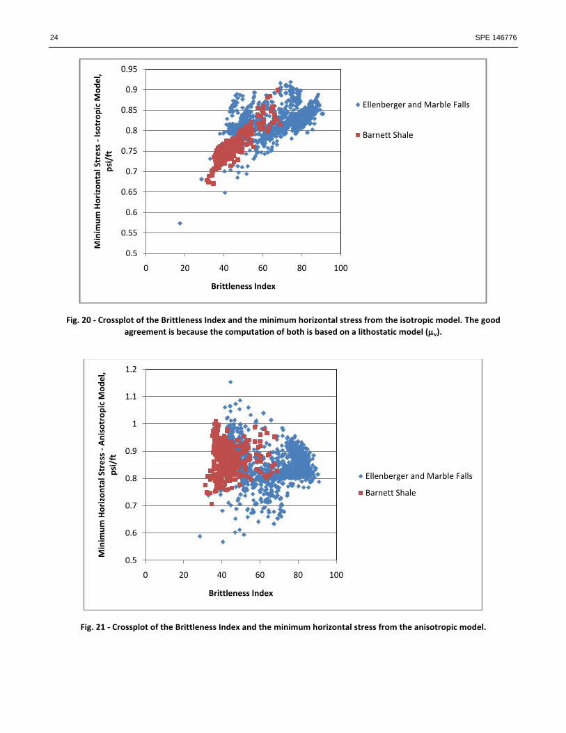
24 SPE 146776

Fig. 20 - Crossplot of the Brittleness Index and the minimum horizontal stress from the isotropic model. The good

agreement is because the computation of both is based on a lithostatic model (v).

Fig. 21 - Crossplot of the Brittleness Index and the minimum horizontal stress from the anisotropic model.

0.5

0.55

0.6

0.65

0.7

0.75

0.8

0.85

0.9

0.95

0 20 40 60 80 100

Min

imu

m H

ori

zon

tal S

tre

ss -

Iso

tro

pic

Mo

de

l, p

si/f

t

Brittleness Index

Ellenberger and Marble Falls

Barnett Shale

0.5

0.6

0.7

0.8

0.9

1

1.1

1.2

0 20 40 60 80 100

Min

imu

m H

ori

zon

tal S

tre

ss -

An

iso

tro

pic

Mo

de

l, p

si/f

t

Brittleness Index

Ellenberger and Marble Falls

Barnett Shale

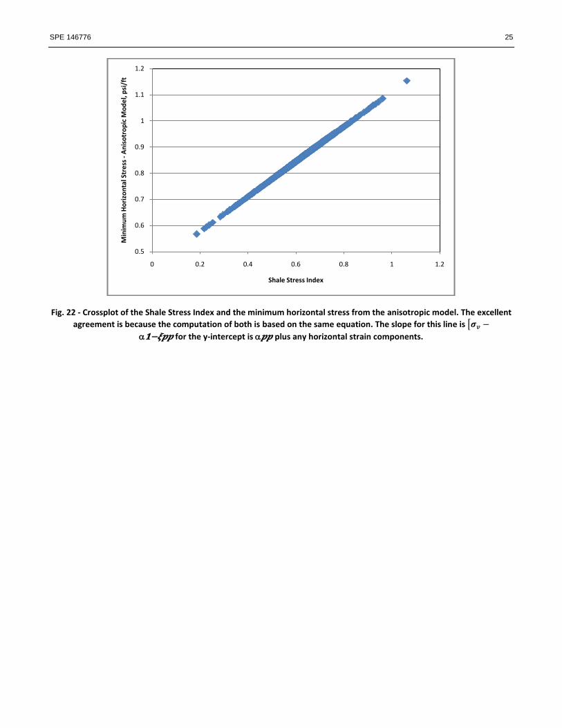
SPE 146776 25

Fig. 22 - Crossplot of the Shale Stress Index and the minimum horizontal stress from the anisotropic model. The excellent

agreement is because the computation of both is based on the same equation. The slope for this line is

for the y-intercept is plus any horizontal strain components.

0.5

0.6

0.7

0.8

0.9

1

1.1

1.2

0 0.2 0.4 0.6 0.8 1 1.2

Min

imu

m H

ori

zon

tal S

tre

ss -

An

iso

tro

pic

Mo

de

l, p

si/f

t

Shale Stress Index