SPE 161184

Modeling and History Matching Hydrocarbon Production from Marcellus Shale using Data Mining and Pattern Recognition Technologies S. Esmaili, A. Kalantari-Dahaghi, SPE, West Virginia University, S.D. Mohaghegh, SPE, Intelligent Solution, Inc. & West Virginia University

Copyright 2012, Society of Petroleum Engineers This paper was prepared for presentation at the SPE Eastern Regional Meeting held in Lexington, Kentucky, USA, 3–5 October 2012. This paper was selected for presentation by an SPE program committee following review of information contained in an abstract submitted by the author(s). Contents of the paper have not been reviewed by the Society of Petroleum Engineers and are subject to correction by the author(s). The material does not necessarily reflect any position of the Society of Petroleum Engineers, its officers, or members. Electronic reproduction, distribution, or storage of any part of this paper without the written consent of the Society of Petroleum Engineers is prohibited. Permission to reproduce in print is restricted to an abstract of not more than 300 words; illustrations may not be copied. The abstract must contain conspicuous acknowledgment of SPE copyright.

Abstract

The Marcellus Shale play has attracted much attention in recent years. Our understanding of the complexities of the flow

mechanism in matrix, sorption process and flow behavior in complex fracture system (natural and hydraulic) still has a long

way to go in this prolific and hydrocarbon rich formation.

In this paper, we present and discuss a novel approach to modeling, history matching of hydrocarbon production from a

Marcellus shale asset in southwestern Pennsylvania using advanced data mining and pattern recognition technologies. In this

new approach instead of imposing our understanding of the flow mechanism, the impact of multi-stage hydraulic fractures,

and the production process on the reservoir model, we allow the production history, well log, and hydraulic fracturing data to

force their will on our model and determine its behavior. The uniqueness of this technology is that it incorporates the so-

called “hard data” directly into the reservoir model, such that the model can be used to optimize the hydraulic fracture

process. The “hard data” refers to field measurements during the hydraulic fracturing process such as fluid and proppant type

and amount, injection pressure and rate as well as proppant concentration.

The study focuses on part of Marcellus shale including 135 wells with multiple pads, different landing targets, well length

and reservoir properties. The full-field history matching process was completed successfully. Artificial Intelligence (AI)-

based model was shown its capability in capturing the production behavior with acceptable accuracy for individual wells and

for the entire field.

Introduction

Shale gas reservoirs pose a tremendous potential resource for future development, and study of these systems is proceeding

apace. Shale gas reservoirs in particular possess many so-called “unconventional” features and considerations, on macro- and

micro-scales of flow (Freeman e al.2011).

Shale reservoirs are characterized by extremely low permeability rocks that have a number of unique attributes, including

high organic content, high clay content, extremely fine grain size, plate-like micro-porosity, little to no macro-porosity, and

coupled Darcy and Fickian flow through the rock matrix.

In contrast with conventional and even tight sandstone gas reservoirs where all the gas in the pore space is free gas, the gas in

shale is stored by compression (as free gas) and by adsorption on the surfaces of the solid material (either organic matter or

minerals) as well (Guo et al.2012).

This combination of traits has led to the evolution of hydraulic fracture stimulation involving high rates, low-viscosities, and

large volumes of proppant. The stimulation design for plays such as Marcellus Shale is drastically different than anything

else that has been performed in the past. It takes large amounts of space, materials, and equipment to treat the Marcellus

2 SPE 161184

Shale to its fullest potential (Houston et al., 2009)

Currently, the Marcellus shale, covering a large area in the northeastern US, is one of the most sought-after shale-gas

resource play in the United States. It has presumably the largest shale-gas deposit in the world, having a potentially

prospective area of 44,000 square miles, containing about 500 TCF of recoverable gas (Engelder, 2009).

This geological formation was known for decades to contain significant amounts of natural gas but was never considered

worthwhile to produce. Uneconomic resources, however, are often transformed into marketable assets by technological

progress (Considine 2009).

Advances in horizontal drilling and multi-stage hydraulic fracturing have made the Marcellus shale reservoir a focal point for

many operators. Nevertheless, our understanding of the complexity associated with the flow mechanism in the natural

fracture and its coupling with the matrix and the induced fracture, impact of geomechanical properties and optimum design of

hydraulic fractures is still a work in progress.

A vibrant and fast-growing literature exists related to various aspects of gas shales, including operational (e.g., drilling,

completion, and production) and technological challenges. The latter mainly involves difficulties in formation

evaluation/characterization, in modeling macro- and micro-scales of gas flow and transport, and in developing reliable

reservoir simulators.

Understanding reservoir properties like lithology, porosity, organic carbon, water saturation and mechanical properties of the

rock, which includes stresses, beforehand and planning completions based on that knowledge is the key to production

optimization. Therefore, the final objective is to increase our ability to integrate proprietary laboratory and petrophysical

measurements with geochemical, geological, petrologic, and geomechanical knowledge, to develop a more solid

understanding of shale plays and to provide better assessments, better predictions, and better models. Reservoir simulation

has played an important role in this aspect. However there are still many challenges to overcome. One is that the physics of

fluid flow in shale rocks haven’t been fully understood, and are undergoing continuous development as the industry learns

more (Lee and Sidle, 2010). Another one is that detailed reservoir simulation is resource intensive and time consuming.

Alternatively, we can apply pattern recognition technology to deal with the complex behaviors of shale reservoirs. In this

paper, we developed an Artificial Intelligence -based model to honor all field measurement data (e.g. production history,

measured reservoir characterizations including geomechanical and geochemical properties) and raw hydraulic fracturing data

like slurry volume, proppant amount and sizes, injection rate etc.)

This provides the operators with an alternate way to history-match, predict and assess reserves in shale gas. The pattern

recognition approach not only has a much faster turnaround time compared to grid-based simulation techniques, but also

good enough accuracy by incorporating all available data compared to analytical and numerical techniques. The integrated

framework enables reservoir engineers to compare and contrast multiple scenarios and propose field development strategies. Top-down Modeling- Pattern Recognition Based Modeling Approach

Pattern recognition is a tool to achieve this goal by finding patterns among non-linear and interdependent parameters involve

in the shale gas development process.

Interest in the research of pattern recognition applications has spawned in recent years. Popular areas include: data mining

(identification of a 'pattern', i.e., a correlation, or an outlier in millions of multidimensional patterns), document classification

(efficient search of text documents), financial forecasting, and biometrics.

Top down modeling is a formalized comprehensive and very first full-field empirical shale model, which take into account all

aspects of shale reservoirs from reservoir characterization to completion etc.

Despite the common practice in shale modeling using a conventional approach, which is usually done at the well level

(Strickland et al.2011), this technique is capable of performing history matching for all individual wells in addition to full

field by taking into account the effect of offset wells.

There are major steps in the development of a Top-down Shale reservoir model, which essentially is an Artificial Intelligent

(AI)-based shale reservoir model.

SPE 161184 3

a. Spatio-temporal database development-The first step in developing a data driven shale model is preparing a

representative spatio-temporal database (data acquisition and preprocessing). The extent at which this spatio-

temporal database actually represents the fluid flow behavior of the reservoir that is being modeled, determines the

potential degree of success in developing a successful model. The nature and class of the AI-based shale reservoir

model is determined by the source of this database. The term spatio-temporal defines the essence of this database

and is inspired from the physics that controls this phenomenon (Mohaghegh 2011) .An extensive data mining and

analysis process should be conducted at this step to fully understand the data that is housed in this database. The data

compilation, curation, quality control and preprocessing is one of the most important and time consuming steps in

developing an AI-based Reservoir Model.

b. Simultaneous training and history matching of the reservoir model- In conventional numerical reservoir

simulation the base model will be modified to match production history, while AI-based reservoir modeling starts

with the static model and try to honor it and not modify it during the history matching process. Instead, we will

analyze and quantify the uncertainties associated with this static model at a later stage in the development. The

model development and history matching in AI-based shale reservoir model are performed simultaneously during

the training process. The main objective is to make sure that the AI-based shale reservoir model learns fluid flow

behavior in the shale reservoir being modeled. The spatio-temporal database developed in the previous step is the

main source of information for building and history matching the AI-based Reservoir Model.

In this work, multilayer neural networks or multilayer perceptions are used (Hykin 1999). These neural networks are

appropriate for pattern recognition purposes in case of dealing with non-linear cases. The neural network consists of

one hidden layer with different number of hidden neurons, which have been optimized based on the number of data

records and the number of inputs in training, calibration and verification process.

It is extremely important to have a clear and robust strategy for validating the predictive capability of the AI-based

Reservoir Model. The model must be validated using completely blind data that has not been used, in any shape or

form, during the development. Both training and calibration datasets that are used during the initial training and

history matching of the model are considered non-blind.

As noted by Mohaghegh (2011), some may argue that the calibration - also known as testing dataset -is also blind.

This argument has some merits but if used during the development of the AI-based shale reservoir model can

compromise validity and predictability of the model and therefore such practices are not recommended.

c. Sensitivity analysis and quantification of uncertainties-During the model development and history matching that

was defined in Step b, the static model is not modified. Lack of such modifications may present a weakness of this

technology, knowing the fact that the static model includes inherent uncertainties. To address this, the AI-based

Reservoir Modeling workflow includes a comprehensive set of sensitivity and uncertainty analyses.

During this step, the developed and history matched model is thoroughly examined against a wide range of changes

in reservoir characteristics and/or operational constraints. The changes in pressure or production rate at each well are

examined against potential modification of any and all the parameters that have been involved in the modeling

process. These sensitivity and uncertainty analyses include single- and combinatorial-parameter sensitivity analyses,

quantification of uncertainties using Monte Carlo simulation methods and finally development of type curves. All

these analyses can be performed on individual wells, groups of wells or for the entire field.

d. Deployment of the model in predictive mode-Similar to any other reservoir simulation model, the trained, history

matched and validated AI-based shale reservoir model is deployed in predictive mode in order to be used for

performing reservoir management and decision making purposes.

AI-based Reservoir Modeling in Marcellus Shale

The study focuses on part of Marcellus shale including 135 wells with multiple pads, different landing targets, well length

and reservoir properties. In this process, all available data including static, dynamic, completion, hydraulic fracturing,

operational constraint etc. has been used for training and validation of the model. A complete list of inputs that are included

in main data set for development of the base model is shown in Figure 1.

The data set includes more than 1,200 hydraulic fracturing stages. Some wells have up to 17 stages of hydraulic fracturing

while others have been fractured with as few as four stages. The perforated lateral length ranges from 1400 to 5600 ft. The

4 SPE 161184

total injected proppant in these wells ranges from a minimum of about 97,000 lbs up to a maximum of about 8,500,000 lbs

and total slurry volume of about 40,000 bbls to 181,000 bbls.

The Porosity of Upper Marcellus varies from 5 to 10 percent while its gross thickness is measured to be between 43 to 114 ft

with a Total Organic Carbon Content (TOC) between 0.8 to 1.7 percent. The reservoir characteristics of Lower Marcellus

includes porosity of 8 to 14 percent, gross thickness between 60 to 120 ft and TOC of 2 to 6 percent.

Figure 1.Data available in the dataset that includes Location & Trajectory, Reservoir Characteristics, Completion, hydraulic fracturing and Production details

Results and Discussion

History matching process using AI-based modeling approach has gone through a process of inclusion and exclusion of

certain parameters based on their impact on model behavior. A flowchart that shows the evolution process of developing the

AI-based Marcellus shale model from base model to best history match model (optimum number of inputs) is illustrated in

Figure 2.

Figure 2.Marcellus shale AI-Based Full-field history matching process

SPE 161184 5

Impact of the Different Input Parameters

Base Model-As illustrated in Figure 2, the base model was built by incorporating all available data, which is listed in Figure

1. This model consists of all raw field data including (well locations, trajectories, static data, completion, hydraulic fracturing

data, production rates, and operational constraints).

Effect of Offset Well-In order to consider the effect of offset well and taking into account any well interference effects, all

aforementioned properties for closest offset well were included in the modeling.

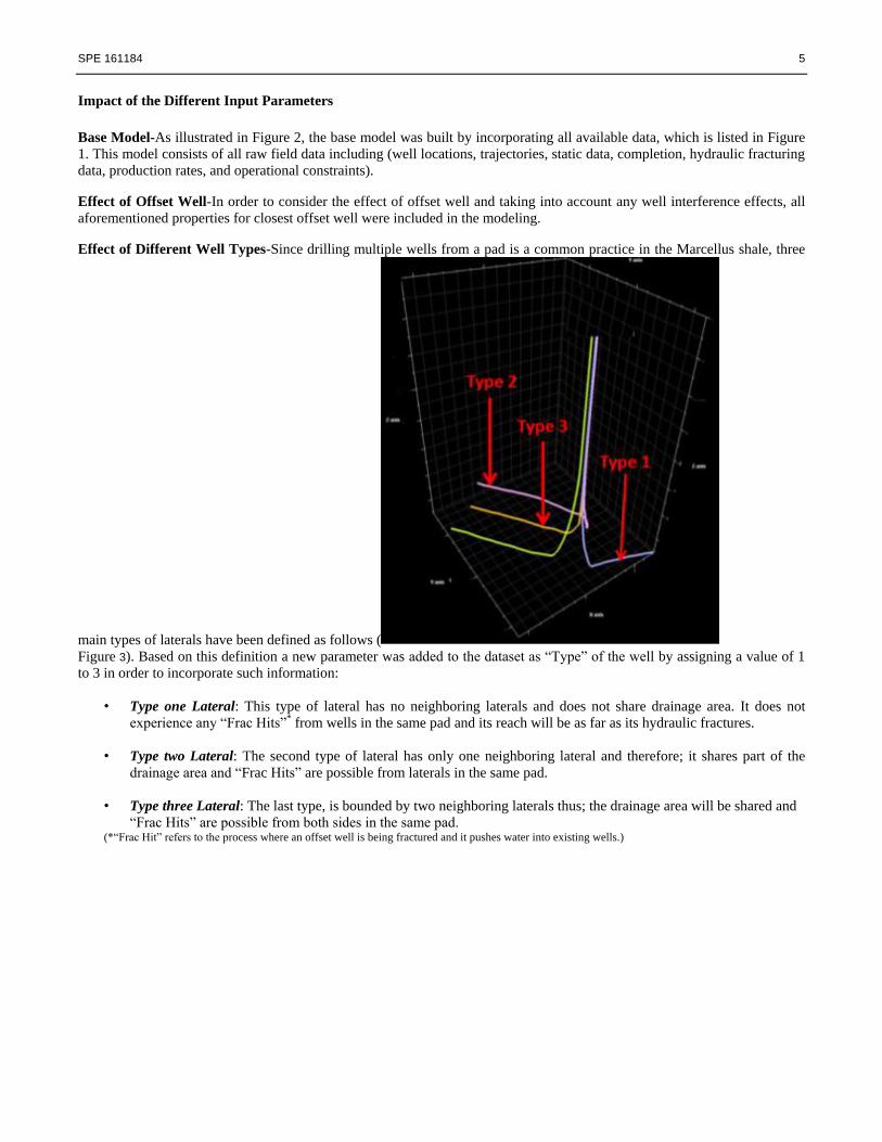
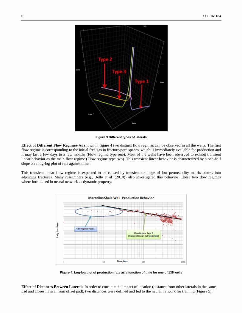
Effect of Different Well Types-Since drilling multiple wells from a pad is a common practice in the Marcellus shale, three

main types of laterals have been defined as follows (

Figure 3). Based on this definition a new parameter was added to the dataset as “Type” of the well by assigning a value of 1

to 3 in order to incorporate such information:

• Type one Lateral: This type of lateral has no neighboring laterals and does not share drainage area. It does not

experience any “Frac Hits”* from wells in the same pad and its reach will be as far as its hydraulic fractures.

• Type two Lateral: The second type of lateral has only one neighboring lateral and therefore; it shares part of the

drainage area and “Frac Hits” are possible from laterals in the same pad.

• Type three Lateral: The last type, is bounded by two neighboring laterals thus; the drainage area will be shared and

“Frac Hits” are possible from both sides in the same pad. (*“Frac Hit” refers to the process where an offset well is being fractured and it pushes water into existing wells.)

6 SPE 161184

Figure 3.Different types of laterals

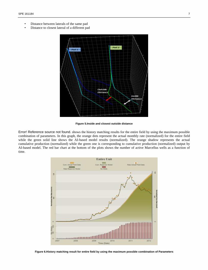
Effect of Different Flow Regimes-As shown in figure 4 two distinct flow regimes can be observed in all the wells. The first

flow regime is corresponding to the initial free gas in fracture/pore spaces, which is immediately available for production and

it may last a few days to a few months (Flow regime type one). Most of the wells have been observed to exhibit transient

linear behavior as the main flow regime (Flow regime type two) .This transient linear behavior is characterized by a one-half

slope on a log-log plot of rate against time.

This transient linear flow regime is expected to be caused by transient drainage of low-permeability matrix blocks into

adjoining fractures. Many researchers (e.g., Bello et al. (2010)) also investigated this behavior. These two flow regimes

where introduced in neural network as dynamic property.

Figure 4. Log-log plot of production rate as a function of time for one of 135 wells

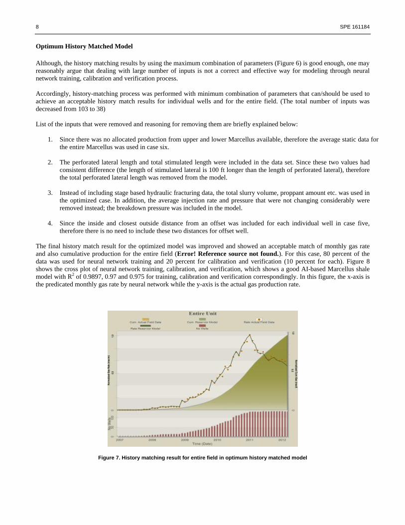
Effect of Distances Between Laterals-In order to consider the impact of location (distance from other laterals in the same

pad and closest lateral from offset pad), two distances were defined and fed to the neural network for training (Figure 5):

SPE 161184 7

• Distance between laterals of the same pad

• Distance to closest lateral of a different pad

Figure 5.Inside and closest outside distance

Error! Reference source not found. shows the history matching results for the entire field by using the maximum possible

combination of parameters. In this graph, the orange dots represent the actual monthly rate (normalized) for the entire field

while the green solid line shows the AI-based model results (normalized). The orange shadow represents the actual

cumulative production (normalized) while the green one is corresponding to cumulative production (normalized) output by

AI-based model. The red bar chart at the bottom of the plots shows the number of active Marcellus wells as a function of

time.

Figure 6.History matching result for entire field by using the maximum possible combination of Parameters

8 SPE 161184

Optimum History Matched Model

Although, the history matching results by using the maximum combination of parameters (Figure 6) is good enough, one may

reasonably argue that dealing with large number of inputs is not a correct and effective way for modeling through neural

network training, calibration and verification process.

Accordingly, history-matching process was performed with minimum combination of parameters that can/should be used to

achieve an acceptable history match results for individual wells and for the entire field. (The total number of inputs was

decreased from 103 to 38)

List of the inputs that were removed and reasoning for removing them are briefly explained below:

1. Since there was no allocated production from upper and lower Marcellus available, therefore the average static data for

the entire Marcellus was used in case six.

2. The perforated lateral length and total stimulated length were included in the data set. Since these two values had

consistent difference (the length of stimulated lateral is 100 ft longer than the length of perforated lateral), therefore

the total perforated lateral length was removed from the model.

3. Instead of including stage based hydraulic fracturing data, the total slurry volume, proppant amount etc. was used in

the optimized case. In addition, the average injection rate and pressure that were not changing considerably were

removed instead; the breakdown pressure was included in the model.

4. Since the inside and closest outside distance from an offset was included for each individual well in case five,

therefore there is no need to include these two distances for offset well.

The final history match result for the optimized model was improved and showed an acceptable match of monthly gas rate

and also cumulative production for the entire field (Error! Reference source not found.). For this case, 80 percent of the

data was used for neural network training and 20 percent for calibration and verification (10 percent for each). Figure 8

shows the cross plot of neural network training, calibration, and verification, which shows a good AI-based Marcellus shale

model with R2 of 0.9897, 0.97 and 0.975 for training, calibration and verification correspondingly. In this figure, the x-axis is

the predicated monthly gas rate by neural network while the y-axis is the actual gas production rate.

Figure 7. History matching result for entire field in optimum history matched model

SPE 161184 9

Figure 8-Neural network training, calibration, and verification cross plots

Figure 9 shows the list of inputs that were used in optimum history matched model.

Figure 9. List of the inputs in optimum history matched model

Figure 10 shows two wells with the best and worst history matching results in optimum history matched model. As it has

shown in this figure, the erratic behavior of the well with worst result could not be captured by AI-base model, even though

the trend was followed.

Figure 10: The best (Left) and worst (Right) history matching results in optimum history matched model

Error Calculation

10 SPE 161184

The error percentage of monthly gas production rate for all 135 wells was calculated using the following equation:

√∑ (

)

Eqn.1

Where:

is the predicted production by TDM (AI-based model)

is the Actual Field data

is the measured maximum change in actual production data

is the number of month of production

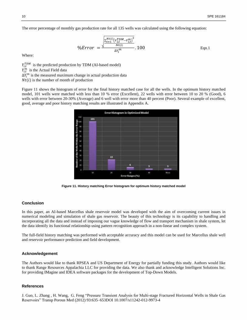
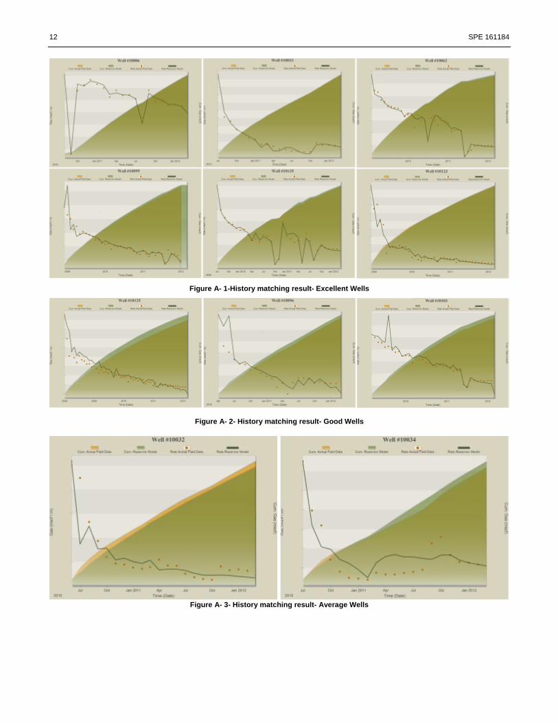
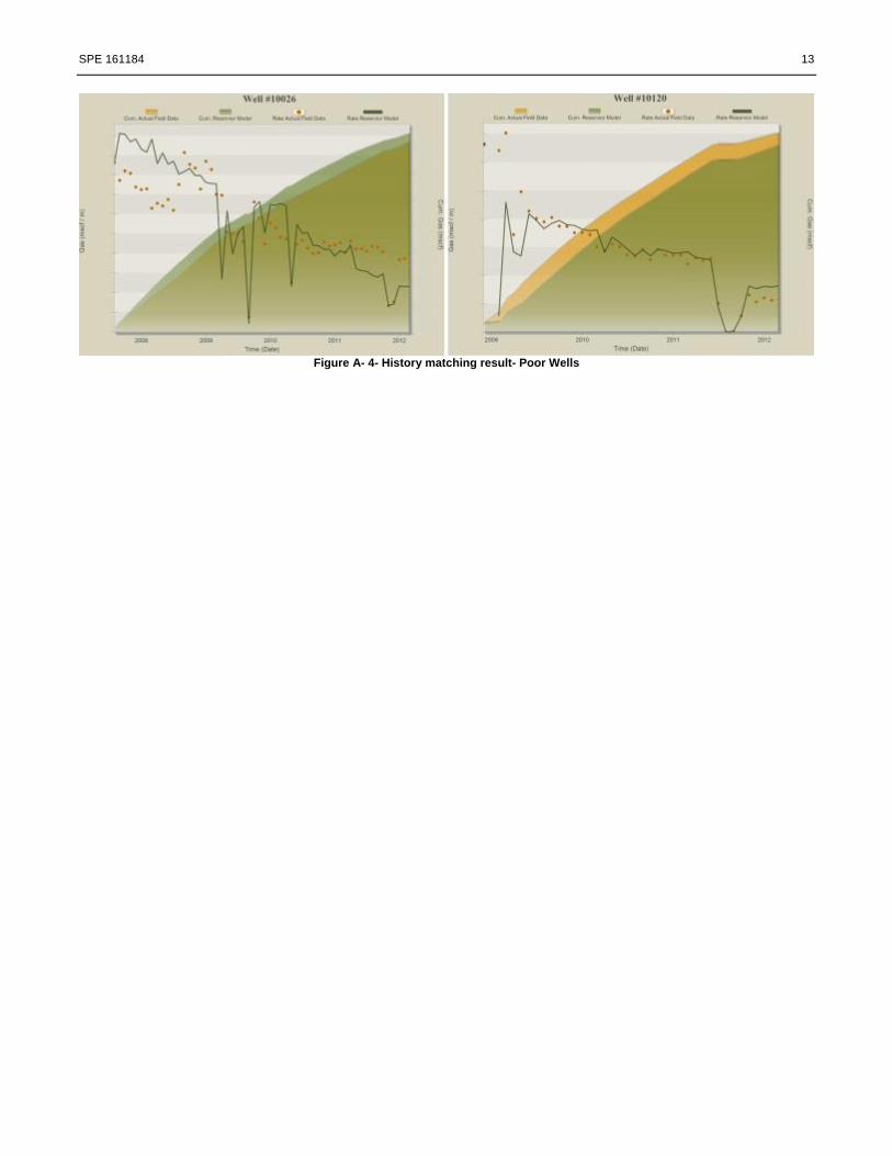
Figure 11 shows the histogram of error for the final history matched case for all the wells. In the optimum history matched

model, 101 wells were matched with less than 10 % error (Excellent), 22 wells with error between 10 to 20 % (Good), 6

wells with error between 20-30% (Average) and 6 well with error more than 40 percent (Poor). Several example of excellent,

good, average and poor history matching results are illustrated in Appendix A.

Figure 11. History matching Error histogram for optimum history matched model

Conclusion

In this paper, an AI-based Marcellus shale reservoir model was developed with the aim of overcoming current issues in

numerical modeling and simulation of shale gas reservoir. The beauty of this technology is its capability to handling and

incorporating all the data and instead of imposing our vague knowledge of flow and transport mechanism in shale system, let

the data identify its functional relationship using pattern recognition approach in a non-linear and complex system.

The full-field history matching was performed with acceptable accuracy and this model can be used for Marcellus shale well

and reservoir performance prediction and field development.

Acknowledgement The Authors would like to thank RPSEA and US Department of Energy for partially funding this study. Authors would like

to thank Range Resources Appalachia LLC for providing the data. We also thank and acknowledge Intelligent Solutions Inc.

for providing IMagine and IDEA software packages for the development of Top-Down Models.

References

J. Guo, L. Zhang , H. Wang, G. Feng “Pressure Transient Analysis for Multi-stage Fractured Horizontal Wells in Shale Gas

Reservoirs” Transp Porous Med (2012) 93:635–653DOI 10.1007/s11242-012-9973-4

SPE 161184 11

C. M. Freeman · G. J. Moridis · T. A. Blasingame” A Numerical Study of Microscale Flow Behavior in Tight Gas and Shale

Gas Reservoir Systems” Transp Porous Med (2011) 90:253–268 DOI 10.1007/s11242-011-9761-6

T. Engelder, 2009, Marcellus 2008: Report card on the breakout year for gas production in the Appalachian Basin: Fort

Worth Basin Oil and Gas.

T. Considine, R. Watson, R. Entler, J. Sparks. “An Emerging Giant: Prospects and Economic Impacts of Developing the

Marcellus Shale Natural Gas Play” State College: EME Department, PSU, 2009.

J .Lee, and R. Sidle, Texas A&M “Gas-Reserves Estimation in Resource Plays” SPE Economics & Management Journal,

Volume 2, Number 2, 2010

S.D. Mohaghegh:” Reservoir simulation and modeling based on artificial intelligence and data mining (AI&DM)” Journal of

Natural Gas Science and Engineering, Elsevier B.V., 2011

N. Houston, M. Blauch, and D. Weaver, III, Superior Well Services, Inc.; and David S. Miller, BLX, Inc.; Dave O’Hara,

Snyder Brothers, Inc.:” Fracture-Stimulation in the Marcellus Shale-Lessons Learned in Fluid Selection and Execution” SPE

125987, SPE Eastern Regional Meeting, 23-25 September 2009, Charleston, West Virginia, USA

R.O. Bello and R.A. Wattenbarger, Texas A&M University:” Modeling and Analysis of Shale Gas Production with a Skin

Effect” Journal of Canadian Petroleum Technology (JCPT) December 2010, Volume 49, No. 12

Appendix a: Example of Excellent, Good, Average, and Poor History matching Results

12 SPE 161184

Figure A- 1-History matching result- Excellent Wells

Figure A- 2- History matching result- Good Wells

Figure A- 3- History matching result- Average Wells

SPE 161184 13

Figure A- 4- History matching result- Poor Wells