spe 84276 accounting for interpreted well test pore

Copyright 2003, Society of Petroleum Engineers Inc. This paper was prepared for presentation at the SPE Annual Technical Conference and Exhibition held in Denver, Colorado, U.S.A., 5 – 8 October 2003. This paper was selected for presentation by an SPE Program Committee following review of information contained in an abstract submitted by the author(s). Contents of the paper, as presented, have not been reviewed by the Society of Petroleum Engineers and are subject to correction by the author(s). The material, as presented, does not necessarily reflect any position of the Society of Petroleum Engineers, its officers, or members. Papers presented at SPE meetings are subject to publication review by Editorial Committees of the Society of Petroleum Engineers. Electronic reproduction, distribution, or storage of any part of this paper for commercial purposes without the written consent of the Society of Petroleum Engineers is prohibited. Permission to reproduce in print is restricted to an abstract of not more than 300 words; illustrations may not be copied. The abstract must contain conspicuous acknowledgment of where and by whom the paper was presented. Write Librarian, SPE, P.O. Box 833836, Richardson, TX 75083-3836, U.S.A., fax 01-972-952-9435.

Abstract Optimal reservoir management requires reliable reservoir performance forecasts with as little uncertainty as possible. There is a need for improved techniques for dynamic data integration to construct realistic reservoir models by using geostatistical techniques. This paper gives a method to create porosity models that honor interpreted pore volumes from well test data. Well porosity data, seismic data and well test results are integrated in sequential simulation. Seismic data is modified iteratively until the co-simulated porosity matches the interpreted well test pore volume. A number of examples are shown. Introduction There are many data that can be used to constrain reservoir models including core data, well logs, seismic and production data. There are few wells during reservoir exploration. Seismic data is areally extensive. The large-scale information provided by seismic data is accounted for in the structural framework and facies model. Seismic may also provide additional information on large-scale porosity variations within the facies.

Production data are extraordinarily important because they are direct observations of reservoir performance. Any reliable reservoir characterization study should account for these dynamic data [1,2].

Well test data is one kind of production data that can provide average porosity and permeability in some volume near the well. In fact, average porosity is an input to well test analysis, but it must be adjusted during well test interpretation in order to make the actual pressure curves and theoretical type curves match better. Because effective pore volume in the area around a well is a basic concept used in well test model and can be calculated by multiplying average effective porosity by formation thickness and relevant area, the basic idea of this paper is to account for the pore volume from well

test data by slight modifications to seismic data when co-simulating porosity. This makes the model more predictive since it matches interpreted flow data and decreases uncertainty in the porosity model. Methodology Hard data include the facies assignments, porosity, and permeability observations taken from core and well logs that provide reliable measurements at the scale we are modeling. All other data including seismic data and production history are called soft data and must be calibrated to the hard data.

Seismic data are frequently used as secondary data for co-simulation of porosity based on the relationship between porosity and seismic [3,4,5]. The seismic data are often impedance values from seismic inversion or some other attribute if an inversion has not been undertaken. The sole calibration parameter is the correlation coefficient between the Gaussian transform of porosity and the Gaussian transform of seismic. Seismic data constrains the spatial distribution of porosity. Well test data can be seen as additional soft data that the porosity model must reproduce [6,7]. The two soft data (seismic data and well test) must be considered simultaneously. Two significant complexities make this difficult. First, the volume scale difference between the hard data, the modeling scale, the seismic scale, and the well test make it very difficult to quantify the relationship between the data types. Second, the cross correlation or redundancy between the different soft data must be modeled at the same time as their correlation to the hard data. Finally, porosity does not average linearly after Gaussian transformation. For these reasons, a full cokriging approach is not practical.

It is conceptually straightforward and practically efficient to slightly modify or update the seismic data to carry the information of the well test data. Using the updated seismic data as secondary data for Gaussian simulation will decrease the uncertainty of the results.

Consider the estimation of an unknown Gaussian transform of porosity z*(u) at an unsampled location u by:

)()()(*1

uuu yzzn

iii µλ += ∑

=

(1)

The collocated seismic value is denoted y(u). The n+1

weights ( µλ ;,,2,1, nii ⋅⋅⋅= ) are calculated by the well known collocated cokriging equations:

SPE 84276

Accounting for Interpreted Well Test Pore Volumes in Reservoir Modeling Linan Zhang, SPE, Luciane B. Cunha, SPE, and Clayton V. Deutsch, SPE, University of Alberta

2 Accounting for Interpreted Well Test Pore Volumes in Reservoir Modeling SPE 84276

)()()(1

uuuuuu −=−⋅⋅+−∑=

ii

n

jjij CCC ρµλ

for ni ,1,2, ⋅⋅⋅=

ρµρλ =+−∑=

n

jjij C

1)( uu

The estimation variance or kriging variance is given by:

µρλσ −−= ∑=

)()(1

2 uuu i

n

iiK C (3)

Assuming multivariate Gaussianity permits the distribution

of uncertainty at u to be predicted as Gaussian in shape with mean z*(u) and variance )(2 uKσ . Simulation proceeds by drawing from such conditional distributions with increasing levels of conditioning. A Gaussian value is drawn:

)(*)()()( )(1)( uuu zpGz K

ll +⋅= − σ (4)

where G-1 is the Gaussian quartile function and p(l) is a uniform pseudo random number.

The porosity is established by back transformation

)))((()( )(1)( uu ll zGF −= φφ (5)

The seismic data y(u) value in Equation 1 can be modified within some allowable range to ensure that the simulated realization reproduces the average porosity from the well test interpretation.

Matching pressure transient well test data requires an average porosity for a specified areal geometry and reservoir thickness. The effective porosity is considered to be an input parameter; however, it is often adjusted in the well test interpretation process. This provides additional data for reservoir characterization. The porosity values and geometry are denoted:

( i

WT

i V,φ ) for WTni ,,2,1 ⋅⋅⋅=

where Vi represents a 3-D volume defined by upper and lower surfaces and inner/outer drainage radii.

There may be multiple annular regions around the same well. The average porosity of a geostatistical realization is written by:

∑∈

=iV

jl

i

li N

juu )(1 )()( φφ

for WTni ,1,2, ⋅⋅⋅= ; Ll ,1,2, ⋅⋅⋅= (6)

The average values from the simulated realizations should

reasonably match the average effective porosity from well test interpretation.

Of course, the well test data provides a total connected pore volume or “storativity” and not just an average porosity; however, if we match the average porosity within the correct volume (area and thickness) we will also match the storativity.

WTiφ is compared with )(l

iφ . If they do not match, the following factor f is used to update the Gaussian transforms of the seismic data:

)1)((sign1)(

)( −+=l

i

WT

ilif

φφ

ρ

for WTni ,1,2, ⋅⋅⋅= ; Ll ,1,2, ⋅⋅⋅= (7)

where 1, for ρ > 0

sign( ρ ) = 0, for ρ = 0 -1, for ρ < 0

The seismic data is modified by :

)()( 1)(j

klij

k yfy uu −⋅=

for ,ij V∈∀u WTni ,1,2, ⋅⋅⋅= (8)

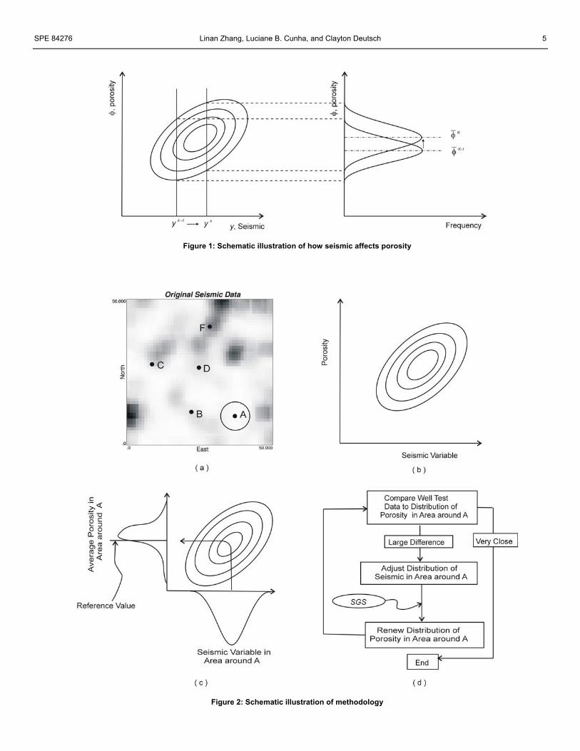
The seismic data are adjusted so that the porosity moves in the right direction. For example, an increase in y in Figure 1 results in an increase in the expected value of porosity.

Co-simulation will give new simulated porosity values with the new seismic data. The seismic is updated until the simulated porosity )(l

iφ matches the well test porosity WTiφ .

This procedure must be applied iteratively and repeatedly for each realization.

Iteration number k = 0 is corresponding to unadjusted seismic data.

Figure 2 gives a schematic explanation for the methodology. Figure 2(a) is a map of seismic data with wells posted on it. The area in the circle indicates the area of influence of the well test at A. There is a relationship between porosity and seismic data and the correlation coefficient is shown in Figure 2(b). Using seismic data as secondary data in co-simulation, the porosity distributions are changed to use the seismic as drawn as Figure 2(c). In most cases, the simulated porosity does not match the reference value from the well test and the simulated value has a larger uncertainty. Using the interpreted average porosity from well test can reduce the uncertainty and increase the accuracy for the simulated value. The iterative procedure is shown in Figure 2(d).

The porosity is simulated with SGS (Sequential Gaussian Simulation)[8] using the latest grid of seismic data. The average porosity values are calculated and compared to the well test derived average values. The seismic values are updated until the simulated average values match the average porosity interpreted from well test.

)2(

SPE 84276 Linan Zhang, Luciane B. Cunha, and Clayton Deutsch 3

Application A reference porosity field with 50x50 grid cells is shown in Figure 2(a). There are 6 wells in it and 5 of them have well test data and corresponding connected volumes. Pressure transient data and their interpretation are uncertain; therefore, the reference values were assigned an error variance of 5%.

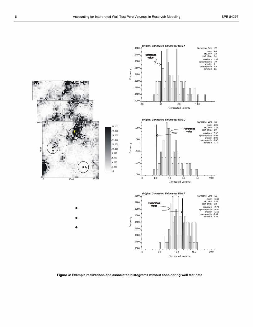
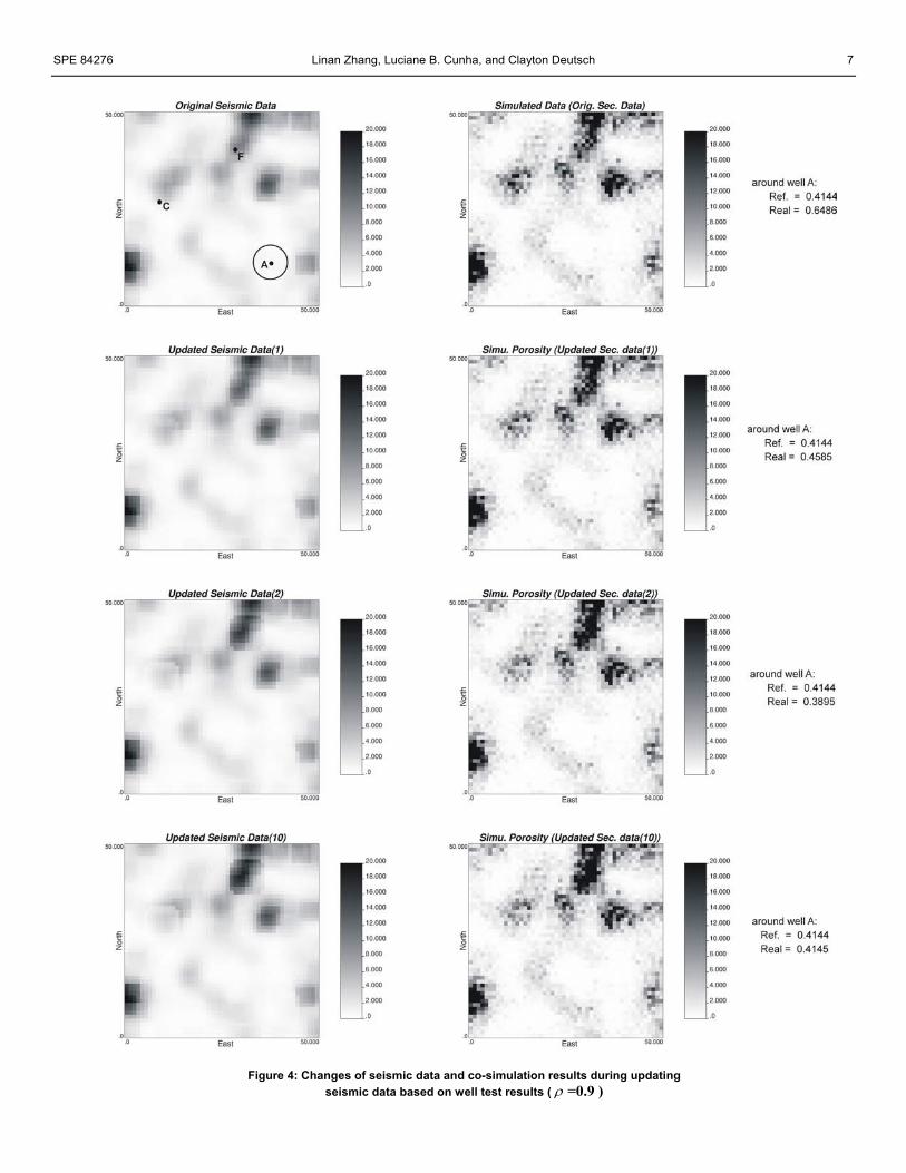
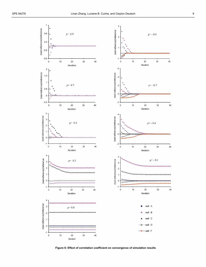
The standard GSLIB data set “true.dat” and related secondary data “ydata.dat” were used for this first example [8]. The units are not exactly for porosity; however, the methodology is insensitive to the exact units. Any volumetric average could be considered. Using original seismic as secondary data in co-simulation. To check how close the simulated connected volumes are to the reference well test values, one hundred realizations of porosity were generated by Sequential Gaussian Simulation with an isotropic spherical variogram and the original seismic data as secondary data. Figure 3 gives the histograms of connected volumes for three wells based on the 100 realizations. Well A is located where seismic values are low. Well F is located where seismic values are high. Well C is located at the interface between low and high seismic value regions. The reference connected volumes from the reference well test values are also shown in the Figure. We see a large uncertainty for the connected volumes from simulated porosity. The probability of simulating porosity that just happens to match the reference value is low. Changes of simulated connected volume versus updated seismic data. Figure 4 shows pixel plots of seismic and simulated porosity as well as connected volumes for the initial realization, first, second, and tenth iteration with the correlation coefficient of 0.9. The changes can be seen in the plots. When seismic data is updated 10 times, the connected volume calculated from the simulated values is very close to the reference value ( “Ref.” means the reference connected volume from well tests and “Real” means the connected volume from simulated porosity). The method appears to work for the Well A. Changes of factor and relative error versus iteration. Figure 5 shows the factor and the relative difference between the reference and simulated values versus iteration for correlation coefficients between porosity and seismic of 0.9, -0.9, 0.7 and –0.7, respectively. The connected volumes converge to the reference values in both cases. For positive correlation coefficient, the factor should be less than one when the reference value is smaller than the simulated porosity. The factor should be larger than one when the reference value is larger than the simulated porosity. For negative correlation coefficient, the factor is larger than one when the reference value is smaller than the simulated value. The factor should be less than one when the reference value is larger than the simulated value. The factor should converge to one when the connected volumes from the simulated porosity converge to the reference values. Effect of correlation coefficient on convergence of results. The correlation coefficient between porosity and seismic data can affect the convergence of results. Correlation coefficients -0.9, -0.7, -0.4, -0.1, 0, 0.1, 0.4, 0.7 and 0.9 were studied. Figure 6 shows the effect of correlation coefficient on the convergence of simulated connected volume. In general, the higher the absolute value of the correlation coefficient, the

quicker the convergence of the simulated values to the reference values. For the same absolute values, the connected volumes for negative correlation coefficients converge more slowly than those for positive correlation coefficients. This is because the porosity and seismic data (from the GSLIB data sets) are actually positively correlated.

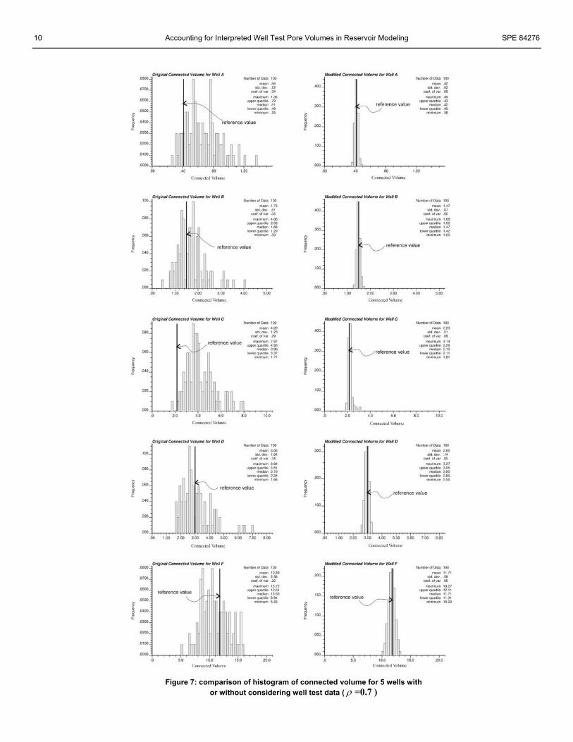
The simulated values can not converge to the reference values when the correlation coefficient is close to zero, e.g. -0.1, 0, 0.1. This is expected. The seismic values are given no weight (µ=0) when the correlation is zero; any changes to seismic would have no affect whatsoever on the connected volume. Comparison of histograms for connected volume with and without considering well test data. 100 realizations considering the well test data were generated with the correlation coefficient of 0.7. For each realization, a reference connected volume is drawn from a Gaussian distribution with a mean equal to the reference value and a variance 0.05. This is done to account for error or uncertainty in the interpreted well test storativity. Any value could be used

Figure 7 shows the comparison of histograms for connected volumes around 5 wells with and without considering well test data. The figures on the left side correspond to no well test data and the figures on the right side correspond to those considering well test data. The uncertainty decreases when the well test data are used to update the seismic data.

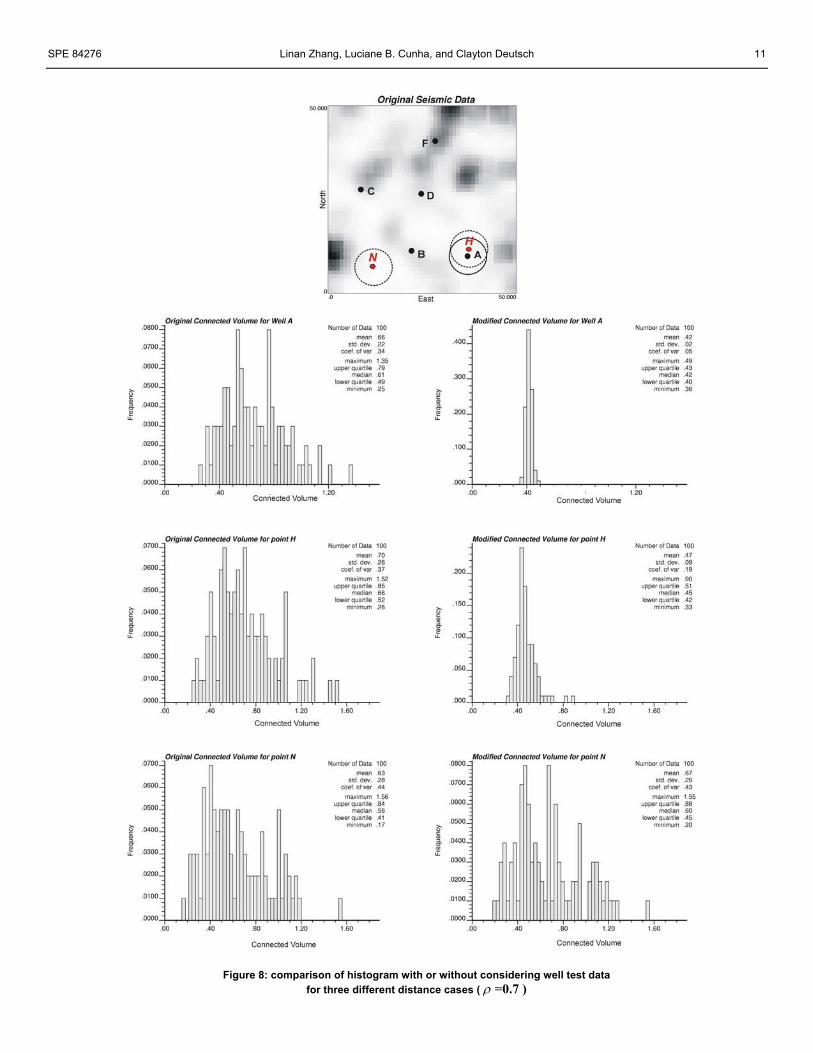
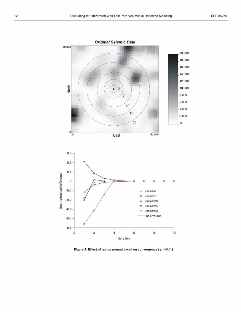
Figure 8 shows the histograms for connected volumes with and without considering well test data in three areas: at the well, near the well and outside the influence of the well. The figures on the left side correspond to no well test data and the figures on the right side correspond to the realizations considering well test data. Modifying seismic data according to well test data reduces the uncertainty of simulated porosity near the well, but does not affect the simulated porosity values far away from the well. The effect of geometry around a well on the result convergence. The geometry of the well test volume around a well affects the connected volume and the simulated porosity values with the correlation coefficient of 0.7. Assuming the area influenced by a well is circular, different radii are used to represent different geometries. Figure 9 shows the effect of different radii on the convergence of connected volumes. The connected volumes converge to the reference values for all radii. Discussion

The changes to seismic data to reproduce well test data should be small. If the changes are large, then it is important to look for alternative explanations such as (1) errors in well test modeling (2) incorrect structure, or (3) biased Geostatistical modeling parameters. The proposed procedure could be used to detect inconsistent modeling parameters.

The changes to the secondary variable could be spread smoothly to the entire reservoir area. The technique would then resemble the sequential self-calibration (SSC)[9] and gradual deformation techniques [10].

The procedure could also be adapted to permeability modeling where the goal is to match interpreted k-h values.


Conclusion and Future Work This paper presents a methodology for generating porosity models honoring well test results. The method is to use seismic data as secondary data in Sequential Gaussian Simulation and the effective connected volume interpreted from well test data as additional soft data to update seismic data. The methodology has been demonstrated with some synthetic examples. The results showed that the methodology is able to decrease the porosity uncertainty derived from porosity-seismic co-simulation due to the constraint of the well test data.

Although some sensitivity studies have been performed to investigate how robust the methodology is, there are some important issues that warrant further research. The application of smoothing techniques on the updated seismic map should be explored. The allowable deviation of seismic data is an important aspect to be investigated. Additional application of this methodology to real reservoirs is a priority. Nomenclature

C(h) = covariance (1- )(hγ ) of the Gaussian-transformed porosity

f (l) = factor used to update the Gaussian transforms of the seismic data( Ll ,1,2, ⋅⋅⋅= )

φF = porosity distribution G = standard Gaussian distribution. i = location index with porosity data or well test

data j = cell index l = realization index k = iteration number L = number of realizations n = number of sampled porosity data

nWT = number of wells with well test data Ni = the number of cells within the specified

volume (uj∈Vi , i= WTn,,2,1 ⋅⋅⋅ ). p(l) = a random number seed ( Ll ,1,2, ⋅⋅⋅= ) u = location being estimated ui = sampled location of porosity data

( ni ,1,2, ⋅⋅⋅= )

iV = the connected volume for the affected region by well i ( i= WTn,,2,1 ⋅⋅⋅ )

)(uy = Gaussian-transformed seismic value at the location being estimated

Z(ui) = Gaussian-transformed porosity data at sampled location ui ( ni ,1,2, ⋅⋅⋅= )

Z*(u) = Gaussian-transformed porosity at unsampled location u

z(l)(u) = Gaussian-transformed value of the lth realization of simulated porosity data ( Ll ,1,2, ⋅⋅⋅= )

)(hγ = variogram of the Gaussian-transformed porosity

iλ = weight applied to the ith known porosity data ( ni ,1,2, ⋅⋅⋅= )

µ = weight applied to the seismic data ρ = correlation between Gaussian-transformed

porosity and Gaussian-transformed seismic data.

)(2 uKσ = kriging variance or estimation variance )(l

iφ = average porosity from simulated porosity of the lth resolution in the region affected by well i (i= WTn,,2,1 ⋅⋅⋅ , Ll ,1,2, ⋅⋅⋅= )

WT

iφ = average porosity from well test interpretation in the region affected by well I (i = WTn,,2,1 ⋅⋅⋅ )

References 1. Deutsch C.V.: Geostatistical Reservoir Modeling, Oxford

University Press, New York (2002) 376 pages. 2. Goovaerts, P.: Geostatistics for natural resources evaluation,

Oxford University Press, New York (1997) 483 pages. 3. Bortoli, L. J., Alabert, F., Haas, A. and Journel, A.:

“Constraining stochastic images to seismic data,” GEOSTATISTICS TROIA’92, volume 1, Kluwer Academic publishers, 3300 AA Dordrecht, The Netherland (1993) pp 325-337.

4. Doyen, P. M., Boerand, L. D. den and Pillet W. R.: “Seismic porosity mapping in the Ekofisk Field using a new form of collocated cokriging,” paper SPE 36498 presented at the 1996 SPE Annual Technical conference and exhibition, Denver, Oct.6-9.

5. Xu, W., Tran, T.T., Srivastava, R.M., and Journel, A.G.: “Integrating seismic data in reservoir modeling:The collocated cokriging alternative,” paper SPE 24742 presented in the 67th Annual Technical conference and exhibition, Washington, DC, Oct.1992.

6. Cunha, L.B., Oliver D.S., Render, R.A. and Reynolds, A.C.: “A Hybrid Markov Chain Monte Carlo method for generating permeability fields conditioned to multiwell pressure data and prior information,” paper SPE 36566 presented at the 1996 SPE Annual Technical conference and exhibition, Denver, Oct. 6-9.

7. Landa, J.L. and Horne, R.N.: “Procedure to integrate well test data, reservoir performance history and 4D seismic information into a reservoir description,” paper SPE 38653 presented at the SPE Annual Technical conference and exhibition, San Antonio, TX,, Oct.1997.

8. Deutsch C.V. and Journel A.G.: GSLIB: Geostatistical Software Library: and User’s G uide, second edition, Oxford University Press, New York (1998) 369 pages.

9. Wen, X. H., Deutsch, C. V. and Cullick, A.S.: “High-resolution reservoir models integrating multiplewell production data,” SPEJ (Dec. 1998) pp 344-355.

10. Hu, L.Y.: “Combination of Dependent Realizations within the gradual deformation method,” Mathematical Geology (Nov. 2002) pp 953-964.


Figure 1: Schematic illustration of how seismic affects porosity

Figure 2: Schematic illustration of methodology


Figure 3: Example realizations and associated histograms without considering well test data


Figure 4: Changes of seismic data and co-simulation results during updating

seismic data based on well test results ( ρ =0.9 )


Figure 5: Changes of factor and relative error with iteration


Figure 6: Effect of correlation coefficient on convergence of simulation results


Figure 7: comparison of histogram of connected volume for 5 wells with

or without considering well test data ( ρ =0.7 )


Figure 8: comparison of histogram with or without considering well test data for three different distance cases ( ρ =0.7 )


Figure 9: Effect of radius around a well on convergence ( ρ =0.7 )

spe 84276 accounting for interpreted well test pore

Documents