spe 90108 dynamic reservoir well interaction - ntnu: startside - ntnu
TRANSCRIPT
Copyright 2004, Society of Petroleum Engineers Inc. This paper was prepared for presentation at the SPE Annual Technical Conference and Exhibition held in Houston, Texas, U.S.A., 26–29 September 2004.
This paper was selected for presentation by an SPE Program Committee following review of information contained in a proposal submitted by the author(s). Contents of the paper, as
presented, have not been reviewed by the Society of Petroleum Engineers and are subject to correction by the author(s). The material, as presented, does not necessarily reflect any position of the Society of Petroleum Engineers, its officers, or members. Papers presented at
SPE meetings are subject to publication review by Editorial Committees of the Society of Petroleum Engineers. Electronic reproduction, distribution, or storage of any part of this paper for commercial purposes without the written consent of the Society of Petroleum Engineers is
prohibited. Permission to reproduce in print is restricted to a proposal of not more than 300 words; illustrations may not be copied. The proposal must contain conspicuous acknowledgment of where and by whom the paper was presented. Write Librarian, SPE, P.O.
Box 833836, Richardson, TX 75083-3836, U.S.A., fax 01-972-952-9435.
Abstract
In order to develop smart well control systems for unstable oil
wells, realistic modeling of the dynamics of the well is
essential. Most dynamic well models use a semi-steady state inflow model to describe the inflow of oil and gas from the
reservoir. On the other hand, reservoir models use steady state
lift curves for modeling of the wells. When producing oil from
thin oil rims, this description does not sufficiently describe the
well behavior observed in practice. For this reason, a model was built that describes both the dynamic flow of oil and gas
towards the well bore and the dynamic flow inside the well.
The integrated model provides a realistic description of the
well dynamics on a time scale of minutes, which is the time
scale that is required for development of a control system. As
a result, the integrated model allows the development of model based gas coning control or water coning control schemes, as
well as model based interpretation of well data.
Introduction
Oil producing wells often encounter instabilities during
production. Various types of automatic control systems can be developed in order to prevent unstable operation. Due to the
increasing availability of sensors and actuators applications of
smart well control become gradually more feasible1 2 3. For the
development of smart well control systems realistic modelling
of the dynamic well behaviour is essential. From practical
experience it appears that in several applications the interaction between the reservoir and the well plays a
dominant role in the dynamic behaviour of the well. In order
to still be able to develop control systems for these situations,
the near well bore reservoir was modelled and was integrated
with the well model, resulting in a model describing the dynamic interaction between reservoir and well.
________________________ * Now with Scandpower Petroleum Technolgy AS
One condition for unstable oil production occurs at low gas lift rates and is known as heading. Although steady-state flow
analysis sometimes indicates most efficient production at these
gas lift rate, dynamic analysis predicts cyclic variations of
liquid and gas production. This often results in periods with
reduced or even no liquid production, followed by large peaks of liquid and gas.
Another situation where unstable production occurs, is when
oil is produced from a thin oil rim, where the gas cap is close
to the perforations of the well. When increasing the drawdown
a cone of gas will be formed. Due the formation of a gas cone, not only oil enters the tubing, but also gas will enter the
tubing. In some conditions this can lead to excessive
production of gas, and as a result a decreased or unstable oil
production. In other conditions however a small amount of
cone gas entering the well can create natural gas lift, and will
stimulate oil production rather then disturbing it. For operation of an oil well where the risk of gas coning is present, it is
important to know the conditions that affect the production of
cone gas. Cone formation and production of cone gas is a
dynamic phenomenon, involving both reservoir and well
dynamics. When the well perforations are close to the water layer, also water coning can take place. Also water coning is a
dynamic phenomenon, involving reservoir and well dynamics.
A simulation model was developed with the aim to describe
the main dynamic phenomena that are important for the
development of smart well control systems. This includes the situations mentioned above. The model focusses on the
dynamic interaction between the different subsystems, which
allows some simplifications in the description of the individual
subsystems.
The structure of the model is explained in this paper and typical behaviour indicating reservoir well interaction is
pointed out. The simulation results are compared to the results
where only the dynamics of the well are described and where
the reservoir dynamics are neglected. In addition the model
was validated with field data from a thin oil rim reservoir.
Finally different applications are mentioned how the model can be used for the optimisation of oil production
Model structure
The system investigated consists of a vertical production
tubing, an annulus for the lift gas and the near well bore reservoir region (Fig. A-1, Appendix). A mechanistic model
SPE 90108
Dynamic Reservoir Well Interaction W.L. Sturm, SPE, S.P.C. Belfroid, SPE, O. van Wolfswinkel
*, M.C.A.M. Peters, SPE, F.J.P.C.M.G. Verhelst, SPE
TNO TPD, Delft, The Netherlands
2 SPE 90108
was developed describing the dynamic behaviour of the gas
and oil flow in the reservoir towards the well bore and the
behaviour of the flow in the production tubing. The near well bore region is described with a radial inflow model for both
the oil and gas phase.
The two-phase flow in the tubing is described by means of a
drift-flux model and in the annulus a single phase gas flow is
described.
The different components involved are discussed hereafter.
Dynamic Reservoir Model. The reservoir model comprises a
radial inflow model. In this section of the reservoir it is
assumed that a fully segregated oil and gas phase exists below a cap rock. The segregated black oil and gas layers are coupled
by means of the mass conservation for each phase and the
pressures in each layer. The oil flow in the reservoir is
described by the Darcy equation according to Dake4:
r
pA
kqL ∂
∂−=µ
, (1)
with qL the liquid flow [m3/s], κ the permeability [m2], µ the viscosity [Pa s], A the (effective) flow area, p the pressure and
r the radial distance to the tubing. The gas flow in the reservoir is calculated with the Forscheimer equation:
��
�
�
��
�
�����
��+−−=
drdpkA
qG
ρβµρβ
µ2
2
4112
, (2)
with qG the gas flow [m3/s], ρ the (gas) density [kg/m3] and β the non-Darcy parameter [1/m].
The Gas Oil Contact (GOC) is the location of the dynamic
interface between the gas and oil layer. The GOC is calculated
with the mass conservation for the liquid (oil) phase:
( )r
rq
rt
xA LLL
L ∂∂−=
∂∂ ρρ 1
, (3)
with ρL the oil density and xL the (relative) oil height (0..1), which corresponds to the GOC.
The pressure in the gas layer is determined with the mass conservation for the gas phase:
( )( ) ( )r
rq
rt
xA GL
∂∂−=
∂−∂ ρρ 11
. (4)
The pressure in the liquid layer is related to the pressure in the gas layer and the hydrostatic head:
LLGLghxpp ρ+= , (5)
with h the height of the reservoir section.
With the equations (1) to (5), a radial inflow model was
established, comprising a number of radial sections (rings)
around the well bore. In each radial section the pressure and the GOC is computed, as well as the flow of oil and gas
towards the next radial section. All variables are a function of
time, i.e. the dynamic response is calculated. At the
perforations, the flow area is corrected with the size of the
perforations and the perforation density. The coupling with the tubing is by the inflows of oil and gas from the radial section
next to the well bore towards the production tubing.
At the outside of the radial inflow sections, i.e. the far field, a semi-steady state inflow performance characteristic is
assumed, i.e. a constant productivity index.
Tubing. In the tubing the two-phase flow is modeled by
means of the drift-flux model (Whalley5). In this approach the
relative motion between the two phases is modeled. Furthermore, fully segregation of the two phases is assumed,
so release of gas from the oil due to the decreasing pressure
along the well was neglected, i.e. black oil. All relations were
derived for a single string, vertical well.
The flow velocity of liquid and gas is computed by combining
the impulse balance for the liquid and gas phase and by using
the drift flux model:
( ) ( )bsL
L
L
GuAqC
Cq ⋅+
−−−=
0
011
1
αα
, (6)
with αL the liquid hold-up, and C0 and ubs the drift-flux model parameters (Whalley5, Legius6). The parameters C0 and ubs are
flow regime dependent and several descriptions and values are
known.
The liquid hold up is calculated with the mass balance for the liquid phase:
x
q
At
LL
∂∂
−=∂
∂ 1α (7)
The pressure in the tubing is calculated with the mass balance
for the gas phase:
xA
q
x
q
Ax
q
At
G
G
GL
G
GG
G
GG
∂∂
−∂
∂−
∂∂
−=∂
∂ ραα
ραρρ
(8)
Using the discretization of the equations (6) to (8) the
production tubing is divided in a number of sections, where
for each section the pressure and the hold up was calculated,
as well as the oil and gas flow to the next section.
Annulus. The annulus was modeled similar to the tubing,
however here only one phase is present. The annulus was
divided in a number of sections, and the pressure and gas flow
are computed for each section.
Production Choke. The flow through the production choke is a multiphase flow. The pressure drop over the production
choke was described with: 2
mixturemixturePCqKp ρ=∆ (9)
where KPC is a constant which depends on the effective size of
the restriction (dependent on the valve position).
The flow line pressure downstream of the production choke is
regarded as a constant pressure in the simulations shown in this publication.
SPE 90108 3
Cases indicating interaction between reservoir and well In this section the response behaviour of the system to
different process variations is explained. Subsequently, the
response of the reservoir to a sudden increase in the
drawdown, the response of the reservoir to a sinusoidal
variation in the drawdown, the response of the system to a
variation in the choke setting and the response of the system in the case of heading are treated.
Height of reservoir section h 100 m
Porosity Φ 0.3
Effective permeability (oil and gas)
k 5 10-14
m2
Average reservoir pressure pres 190 bar
Drainage area boundary re 350 m
Well Bore radius rw 0.07 m
Top of the perforated section
xpt 60 m (above bottom of oil rim)
Bottom of the perforated section
xpb 25 m (above bottom of oil rim)
Perforation density rp 0.5
Table 1 Reservoir parameters
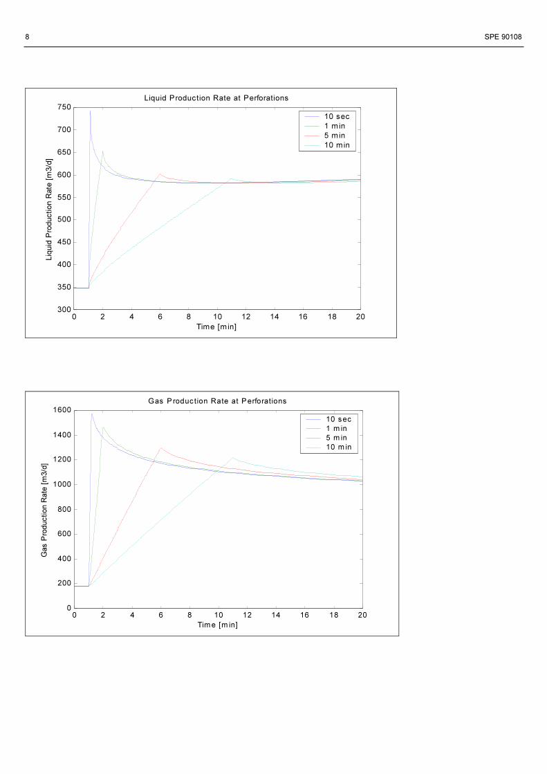
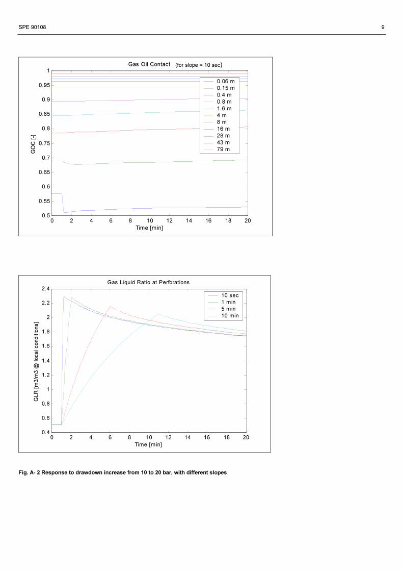
Response to ramp increase of drawdown. While simulating
only the reservoir and imposing an increase in the drawdown
(with different slopes) the behaviour of the oil/gas flows and of the GOC is illustrated in Fig. A-2 (Appendix).
This graph shows that the response of the oil flow depends on
the slope of the ramp of the drawdown. At a slow increase of
the drawdown, the behaviour of the reservoir can be regarded as semi-steady state since the oil flow follows the ramp of the
drawdown. However, when the drawdown increases within 10
seconds, there is a large overshoot in oil production, which
will not be predicted by a semi-steady state reservoir model.
The overshoot is caused by the fact that the pressure in the
dynamic reservoir section closest to the well bore remains higher than the pressure in the well, until enough flow has left
this section, and a new equilibrium arises.
Up to the time this equilibrium exists the oil flow is larger than
the steady state flow that corresponds with this pressure in the
well. When the new equillibrium arises the GOC in the region close to the well bore is lower than far away from the well
bore. In addition the GOC at the end of the response is lower
than at the start of the response, so when increasing the
drawdown the region close to the well bore is drained more
effectively than the region further away from the well bore.
The response of the gas flow also shows an overshoot.
Moreover the GOR response shows an overshoot during a fast
increase of the drawdown. This indicates that the gas
production increases faster than the oil production, due to the
higher mobility of the gas.
When applying a dynamic model for the development of a
well control system, it appears that the reservoir dynamics
have to be taken into account when the control system
operates at a time scale faster than 5 to 10 minutes. The
response of the oil and gas flow to a change of the bottom hole
pressure (due to a change in production choke, or lift gas rate), cannot be regarded as semi-steady state. With a semi-steady
state description of the reservoir the oil flow would exactly
follow the ramp of the bottom hole pressure, while with the
dynamic description there is an overshoot in liquid production
in the first minutes after the ramp starts.
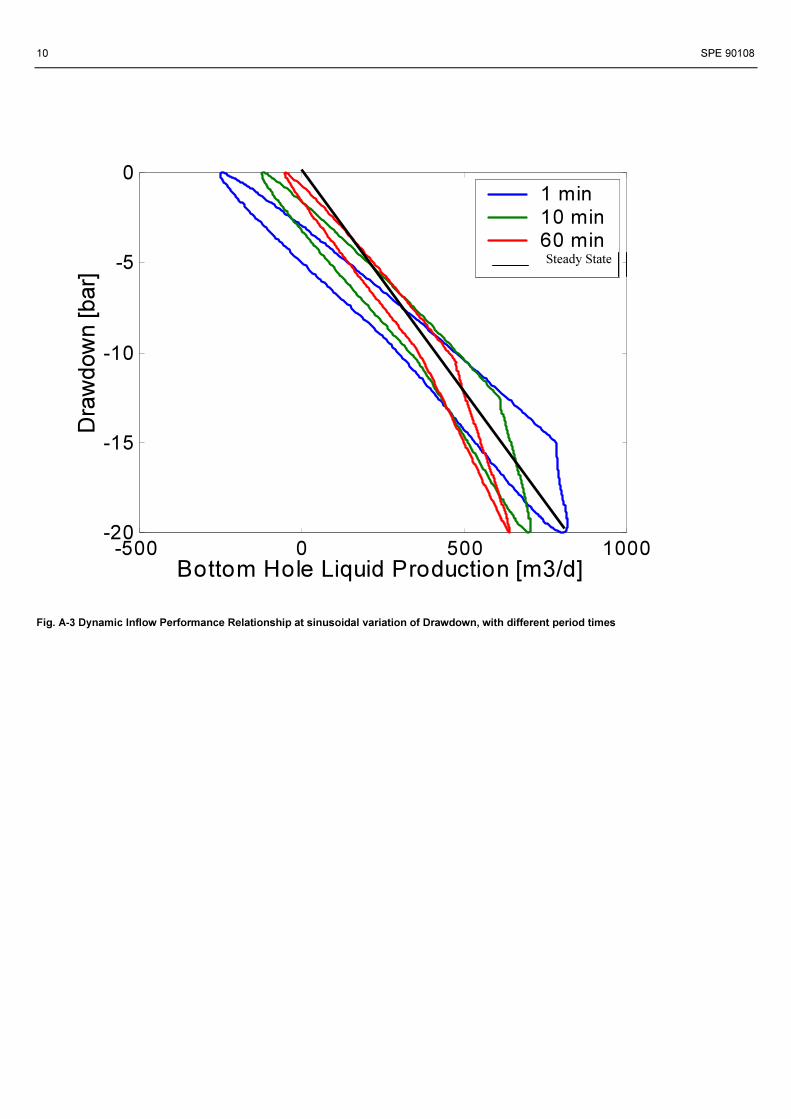
Response to sinusoidal variation of drawdown. To get more
insight in the relevant time scales simulations were carried out
where the drawdown was varied according to a sine wave. Fig.
A-3 (Appendix) shows the dynamic inflow performance
relationship (IPR) at sinusoidal variation of the bottom hole pressure, at different period times. The average bottom hole
pressure was set to 180 bar, so the average drawdown is 10
bar. The amplitude of the bottom hole pressure is 10 bar, so
the drawdown varies between 0 and 20 bar. The straight line
indicates the semi-steady state inflow performance curve.
At a certain point the cone gas is entering the well. At this
point the IPR line is twisted, and the liquid inflow increases
more slowly as a function of drawdown, due to gas entering
the well.
At small drawdowns and at long period times of the drawdown the dynamic IPR is close to the steady behaviour. However,
when the period time is 1 minute the inflow performance can
no longer be regarded as semi-steady state, also when no gas
is entering the well. When an average drawdown of 5 bar with
an amplitude of 5 bar would have been used, (i.e. the drawdown varies from 0 to 10 bar), the dynamic Inflow
Performance curve would be an ellipsis. In this case, it is clear
that at a longer period time the dynamic inflow curve would
approach a straight line (i.e. the semi-steady state IPR),
however, at a short period time the ellipsis shape would differ
significantly from a straight line.
The ellipsis is caused by the phase difference between the
pressure and the flow, due to the dynamic relation between the
pressure and the flow. A fast change in pressure, causes a
delayed change in flow. The faster the pressure change, the
larger the relative delay, so the radius of the ellipsis increases when a smaller period time for the drawdown variations is
applied.
The second phenomena that is observed, is the entering of
cone gas into the well. This occurs when the drawdown has
reached a certain level for a certain time. At a small period time, a larger drawdown is needed for the production of cone
gas, than at a larger period time. When cone gas enters the
well, the production of oil decreases and the production of gas
increases, as is made clear by the inflow curves in Fig. A-3. It
is clear that a steady state IPR is not sufficient to describe the oil production and that instead a dynamic reservoir model
should be used to describe the inflow relations at the right
level of detail.

4 SPE 90108
Response to change production choke setting. At normal
operation, it is expected that if the production choke is opened,
the well head pressure decreases. It will be explained that also different responses are possible due to the effect of reservoir
dynamics.
Fig. A-4 (Appendix) shows a simulation where the response is
displayed to an increase of the production choke opening. In
this picture two different situations are compared. First, the response is calculated for the situation where the well inflow is
described with semi-steady state relations. The inflow of oil is
calculated with a semi-steady state Inflow Performance
Relationship (Dake4):
PI
qS
r
r
kh
qpp L
w
eL
holebottomreservoir=��
�
����
�+−=−
2
1ln
2πµ
(10)
rw is the radius of the well, re is the outer radius of the
reservoir section that is observed. S is the mechanical skin
factor. PI is a constant factor, that takes into account the
average pressure drop over the near well bore reservoir
section, dependent on porosity and permeability of the formation. The reduced permeability close to the well is
accounted for by the mechanical skin factor S.
The inflow of gas is described with the following semi-steady
state relation (Dake4): 222
GGholebottomreservoirFqAqpp +=− (11)
The parameter A describes the pressure loss over the porous
formation, whereas F gives the pressure loss near the tubing,
often accounting for the occurence of turbulent flow. The
parameters A and F are both dependent on porosity and
permeability of the reservoir.
Fig. A-4 shows the response of the dynamic well model,
where the well inflow is described with the above mentioned
semi-steady state reservoir model. This is a classical way of
simulating well dynamics. The response to an increased opening of the production choke is a decrease of the well head
pressure. The production of oil increases fast when the choke
is opened, but later decreases due to the decreased bottom hole
pressure.
The next line in Fig. A-4 shows the response when also the reservoir dynamics are taken into account. Also in this
situation the well head pressure decreases fast after opening
the production choke. The bottom hole pressure decreases
from 100 to 70 bar. At the start of the simulation the GOC is
above the perforations, so no cone gas is entering the well.
Due to the increased drawdown the GOC migrates to a lower position, which causes cone gas flowing into the well. This
increased gas flow causes the well head pressure to increase,
because the pressure drop over the production choke rises, due
to the increased flow through the choke. As a result the
response of the well head pressure to opening the production
choke, is first a decrease of the well head pressure, and after some time an increase of the well head pressure.
In the simulation with the steady state model the gas flow at
the start of the simulation is not zero, because the semi-steady
state relation for gas inflow does not take into account the
formation of a cone.
Again here a dynamic well model, in combination with a
semi-steady state reservoir model, does not sufficiently the
describe the phenomena that take place on a short time scale.
Since this is the time scale that is important for control system
development, the semi-steady model is not sufficient for the
development of well control schemes, and instead the integrated reservoir and well model provides a better
description of the relevant behaviour.
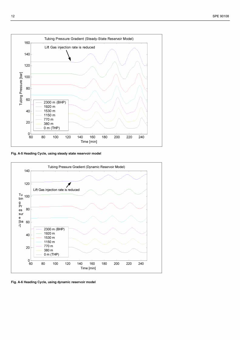
Well performance during heading instability. In gas lifted
wells, instability in the oil production may occur when the lift gas injection rate is too low. This effect is known as heading
instability and is caused by the interaction between the flow
dynamics in the annulus and in the tubing. When heading
instability occurs a cyclic variation of oil flow and well head
pressure is observed. It is interesting to analyze the effect of
dynamic reservoir modelling on the well behaviour during a heading cycle. For this reason two simulations were carried
out. In the first simulation the semi-steady state reservoir
model was used (equation (10)). The result of this simulation
is indicated in Fig. A-5 (Appendix). After 125 minutes, the lift
gas injection rate was reduced. As a result, the heading cycle
occurs, and the well head pressure oscillates with a slowly increasing amplitude. Next, a second simulation was carried
out, where the dynamic reservoir model replaced the semi-
steady state reservoir model. The results of this simulation are
illustrated in Fig. A-6 (Appendix). Again after 125 minutes the
lift gas injection rate was reduced to exactly the same value as was used in the first simulation. Again a heading cycle occurs,
however the amplitude of the changing well head pressure is
much lower than in the first case. This shows that the
dynamics of the reservoir decrease the amplitude of the
pressure fluctuations in the well.
The reason is that due to the short terms variation of the
bottom hole pressure, the oil flow from the reservoir to the
well is not in phase with the pressure fluctuations. The oil flow
is high, when the bottom hole pressure is low and as a result
this causes a stabilizing effect on the well performance.
This example shows that due to the mutual interaction beween
the reservoir and the well the near well bore dynamics cannot
be neglected. So in order to achieve an accurate description of
the dynamic phenomena in the well in this case, the dynamic
interaction with the near well bore reservoir must be taken into
account.
Comparison with field data The developed model was compared with field data. The aim
of the model is to qualitatively describe the behaviour of the
well, as observed by operator personnel. For this reason, data was obtained from a Shell operated field, where gas break
through often is encountered, due to the thin oil rims from
which production takes place. In reality production takes place
from a horizontal well, but the model for a vertical well
already allows to qualitatively investigate the effect of
dynamic interaction of well and reservoir. Therefor only a
SPE 90108 5
qualitative comparison between the model predictions and the
measured data was made. This comparison is shown in
Fig. A-7.
At the start of the measurement there is no oil production. The
well is started up by opening the production choke, and by
opening the lift gas valve. At t=1000 s the production choke
opening is increased, and also the oil and gas flow increase. At
t=3000 s a further increase of gas flow starts, while the (average) production choke opening is not increased. This
increase of gas flow is caused by the formation of a gas cone
in the reservoir. The gas flow gradually increases from 2 to 10
Million standard cubic feet/day during the next 1.5 hours. Due
to the huge increase of gas flow the Gas Oil Ratio increases from 2000 to 6000 scf/bbl.
The well head pressure decreases at t=1000 s when the
production choke is opened, but increases at t=3000 s when
the gasflow increases. At approximately an equal production
choke opening the well head pressure rises from 15 bar at t=2000 s to 35 bar at t=5000 s (1 hour later). In the same
period the oil production has dropped from 3000 bbl/day to
2000 bbl/day.
The problem with the operation of a well where gas coning
takes place, is that at low gas lift rates there is no production of oil. However, while increasing the gas lift rate, there is an
intermediate increase of oil production, but when the cone gas
flow increases the oil production again is strongly reduced. A
feasible operating point for the well can only be obtained by
finding the right combination of lift gas rate and production choke setting. In the example in Fig. A-7 the only way to stop
the increase of cone gas flow is to decrease the production
choke opening, which was done from t=5000 s.
The red line in Fig. A-7 shows the predictions of the
simulation model. The qualitative comparison shows that the dynamic model realistically predicts the measured increase of
gas flow due to the formation of a cone. Since only a
qualitative validation was carried out, the numeric values are
not identical (they are displayed on the right y-axis). Also the
dynamic behaviour of GOR was predicted well. At the start of
the measurement there is a mismatch in the prediction of oil production and well head pressure. However, the dynamic
effects are predicted well, like the initial decrease of the well
head pressure followed by an increase. It is expected that a
better match will be obtained when a dynamic model for flow
towards a horizontal well is built and when segregation of gas
from the oil is incorporated in the model.
Applications The model of dynamic reservoir and well behaviour can be
used as a tool to analyze the behaviour of a well and to
understand the dynamic phenomena that take place. Modification to the well design or well operation, can be
computed and different options can be analyzed before
considering applying a modification to the well.
Moreover, the integrated dynamic model can be used in the
development of smart well control systems. It has been
demonstrated that the integrated model realistically describes
the dynamic behaviour on the same time scale as a well
control system. As a result, the integrated model provides the knowledge of the dynamic behaviour of the well, which is
required for the development of a well control system.
It was shown that the integrated model gives a realistic
description of the instabilities in a gas lifted oil well. In the
development of a control system for an unstable oil well, it appears that the integrated model, where both the reservoir
dynamics and the well dynamics are taken into account, gives
a realistic description of the instabilities that take place in the
well. In addition it was shown that water and gas coning can
be modelled, so for the development of algorithms for gas coning control or water coning control the integrated model
can be used.
Other applications of the dynamic model are to assist the
operator personnel with a tool that predicts the future
behaviour of the well as response to changing choke settings. This can be implemented as an on-line operation support tool,
where the model is coupled to the data acquisition system that
presents the well data. The operator can fill in the adjustments
he wants to use in future (e.g. future production choke setting),
and the operation support tool predicts the future response of
the well (e.g. oil and gas production). The system can also be used as a training tool for operators, to get acquainted with the
dynamic behaviour of a gas coning well.
When the dynamic model is on-line with the data acquisition
system of the well, non-measured parameters (e.g. down hole flow estimation) can be computed during production based on
available measured signals and on detailed knowledge of the
reservoir and well dynamics that are captured by the model
(Bloemen)7. The model has to be brought on line and the
model must be tracked with the well data by applying Kalman
filtering techniques. The same methodology can be used in the interpretation of well test data.
Conclusions A model was build that describes both the flow of oil and gas
towards the well bore and the dynamic flow inside the well.
The Inflow Performance Relationship of the dynamic model was compared to the IPR of a semi-steady state model and it
was demonstrated that at a time scale of minutes, the dynamic
behaviour of the near well bore reservoir significantly affects
the IPR.
Therefore, it is concluded that a dynamic well model, in combination with a semi-steady state well inflow model, is not
sufficient to accurately describe the dynamic phenomena, that
play a role in the development of a control system. Instead it is
required to take into account the interaction between near well
bore reservoir and well, since this can play a dominant role in the description of the dynamic behaviour of the complete
system.
The dynamic model that was developed describes the
dynamics of a vertical well in combination with the dynamics
of the near well bore reservoir. The simulation results were
6 SPE 90108
qualitatively compared to field data. This shows the trends
predicted by the model correspond to the trends observed in
practice. Further model development has to take place to cope with the current mismatch. Future model development will
focus on modelling horizontal wells and segregation of gas.
Possible applications of the dynamic model are analyzing
dynamic well behaviour, development of well control
schemes, or supporting operators and engineers in the operation of a well and interpretation of well data.
Acknowledgment The authors wish to thank Shell Global Solutions for their
valuable contribution to this research project, and for making available measured well data.
Nomenclature A = Area [m2]
C0 = Drift flux model parameter
g = Gravitational constant [m/s2] h = Height of reservoir section
k = Permeability [m2]
KPC = Valve constant [-]
p = Pressure [Pa]
PI = Productivity Index [m3/s/bar]
q = Flow [m3/s] r = Radius [m]
S = Mechanical skin factor [bar]
t = Time [s]
u = Flow velocity [m/s]
x = Relative Height [0..1] α = Hold up [-]
β = non-Darcy parameter [1/m]
µ = Viscosity [Pa s]
ρ = Density [kg/m3]
subscripts L = Liquid (Oil)
G = Gas
bs = Bubble rise velocity (ubs)
mix = Mixture (Liquid and Gas)
e = Outer radius of reservoir section (re)
w = Well radius (rw)
References 1. Jansen, B., Dalsmo M., Nøkleberg, L., Havre, K., Veslemøy,
K., Lemetayer, L.: “Automatic Control of Unstable Gas Lifted
Wells,” SPE paper 56832 presented at the 1999 SPE Annual
Technical Conference and Exhibition, Houston, Texas, Oct.
3-6.
2. Eikrem, G.O., Foss, B., Imsland, L., Hu, B., Golan, M.:
“Stabilization of Gas Lifted Wells,” 15th Triennal World
Congres, Barcelona, Spain, 2002.
3. Hu, B., Golan, M.: “Dynamic Simulator Predicts Gas Lift Well
Instability,” SPE paper 84917 presented at the 2003
International Improved Oil Recovery Conference, Kuala
Lumpur, Oct. 20-21.
4. Dake, L.P.: Fundamentals of Reservoir Engineering, Elsevier
Science, 1978.
5. Whalley, P.B.: Boiling, Condensation and Gas-Liquid Flow,
Department of Engineering Science, published by Oxford
University Press, New York, 1987.
6. Legius, H.J.W.M.: Propagation of Pulsations and Waves in
Two-Phase Pipe Systems, thesis Technical University (TU)
Delft, The Neterlands, Dec. 15, 1997.
7. Bloemen H.H.J., Belfroid S.P.C., Sturm W.L., Verhelst
F.J.P.C.M.G, “Soft Sensing for Gas Lifted Wells”, SPE paper
90370, presented at. the SPE Annual Technical Conference and
Exhibition, Houston, Texas, September 2004

SPE 90108 7
Appendix A
Fig. A-1 Overview of the model for reservoir and well
8 SPE 90108
0 2 4 6 8 10 12 14 16 18 20300
350
400
450
500
550
600
650
700
750
Time [min]
Liq
uid
Pro
du
ctio
n R
ate
[m
3/d
]
Liquid Production Rate at Perforations
10 sec
1 min
5 min
10 min
0 2 4 6 8 10 12 14 16 18 200
200
400
600
800
1000
1200
1400
1600
Time [m in]
Gas P
roduction R
ate
[m
3/d
]
Gas Production Rate at Perforations
10 sec
1 m in
5 m in
10 m in
SPE 90108 9
0 2 4 6 8 10 12 14 16 18 200.5
0.55
0.6
0.65
0.7
0.75
0.8
0.85
0.9
0.95
1Gas Oil Contact
Time [min]
GO
C [
-]
0.06 m
0.15 m
0.4 m
0.8 m
1.6 m
4 m
8 m
16 m
28 m
43 m
79 m
0 2 4 6 8 10 12 14 16 18 200.4
0.6
0.8
1
1.2
1.4
1.6
1.8
2
2.2
2.4Gas Liquid Ratio at Perforations
Time [min]
GLR
[m
3/m
3 @
local conditio
ns]
10 sec
1 min
5 min
10 min
Fig. A- 2 Response to drawdown increase from 10 to 20 bar, with different slopes
(for slope = 10 sec)
10 SPE 90108
Fig. A-3 Dynamic Inflow Performance Relationship at sinusoidal variation of Drawdown, with different period times
-500 0 500 1000-20
-15
-10
-5
0
Bottom Hole Liquid Production [m3/d]
Dra
wd
ow
n [
bar]
1 min
10 min
60 min
Steady State

SPE 90108 11
Fig. A-4 Response to opening production choke
12 SPE 90108
60 80 100 120 140 160 180 200 220 2400
20
40
60
80
100
120
140
160Tubing Pressure Gradient (Steady-State Reservoir Model)
Time [min]
Tubin
g P
ressure
[bar]
2300 m (BHP)
1920 m
1530 m
1150 m
770 m
380 m
0 m (THP)
Lift Gas injection rate is reduced
Fig. A-5 Heading Cycle, using steady state reservoir model
60 80 100 120 140 160 180 200 220 2400
20
40
60
80
100
120
140 Tubing Pressure Gradient (Dynamic Reservoir Model)
Time [min]
Tubing Pressure [bar]
2300 m (BHP)
1920 m
1530 m
1150 m
770 m
380 m
0 m (THP)
Lift Gas injection rate is reduced
Fig. A-6 Heading Cycle, using dynamic reservoir model

SPE 90108 13
Fig. A-7 Qualitative comparison with field data