special edition using oracle8 (imprint: que) author...
TRANSCRIPT

To access the contents, click the chapter and section titles.
Special Edition Using Oracle8 (Imprint: Que) (Publisher: Macmillan Computer Publishing) Author: Nathan Hughes; Willia ISBN: 0789713454
CONTENTSAcknowledgmentsCredits About this book
PART I - Principles of Database Management Systems
Chapter 1 - Databases, DBMS Principles, and the Relational ModelChapter 2 - Logical Database Design and NormalizationChapter 3 - Physical Database Design, Hardware, and Related IssuesChapter 4 - Chapter not available
PART II - The Oracle Database Server
Chapter 5 - The Oracle Instance ArchitectureChapter 6 - The Oracle Database ArchitectureChapter 7 - Exploring the Oracle Environment
PART III - Oracle Interfaces and Utilities
Chapter 8 - SQL*Plus for AdministratorsChapter 9 - Oracle Enterprise ManagerChapter 10 - PL/SQL FundamentalsChapter 11 - Using Stored Subprograms and PackagesChapter 12 - Using Supplied Oracle Database PackagesChapter 13 - Import/ExportChapter 14 - SQL*LoaderChapter 15 - Designer/2000 for Administrators
PART IV - Oracle on the Web

Chapter 16 - Oracle Web Application Server 3.0Chapter 17 - Web Application Server ComponentsChapter 18 - Installing and Configuring the OracleWeb Application Server
PART V - Oracle Networking
Chapter 19 - Oracle Networking Fundamentals20 Chapter - Advanced Oracle Networking
PART VI - Managing the Oracle Database
Chapter 21 - Managing Database StorageChapter 22 - Identifying Heavy Resource UsersChapter 23 - Security ManagementChapter 24 - Backup and RecoveryChapter 25 - Integrity Management
PART VII - Parallel and Distributed Environments
Chapter 26 - Parallel Query ManagementChapter 27 - Parallel Server ManagementChapter 28 - Distributed Database Management
PART VIII - Performance Tuning
Chapter 29 - Performance Tuning FundamentalsChapter 30 - Application TuningChapter 31 - Tuning MemoryChapter 32 - Tuning I/O
APPENDIX A Oracle on UNIX APPENDIX B Oracle on Windows NT APPENDIX C New Features of Oracle8 APPENDIX D Oracle Certification Programs

Table of Contents | Next
Page 5
Contents
Contents at a Glance
Introduction 1
I Principles of Database Management Systems
1 Databases, DBMS Principles, and the Relational Model 92 Logical Database Design and Normalization 193 Physical Database Design, Hardware, and Related Issues 294 The Oracle Solution 43
II The Oracle Database Server
5 The Oracle Instance Architecture 536 The Oracle Database Architecture 737 Exploring the Oracle Environment 93
III Oracle Interfaces and Utilities
8 SQL*Plus for Administrators 1199 Oracle Enterprise Manager 14710 PL/SQL Fundamentals 17311 Using Stored Subprograms and Packages 23912 Using Supplied Oracle Database Packages 27113 Import/Exportv 30514 SQL*Loader 32915 Designer/2000 for Administrators 351

IV Oracle on the Web
16 Oracle Web Application Server 3.0 39317 Web Application Server Components 40118 Installing and Configuring the Oracle Web Application Server 423
V Oracle Networking
19 Oracle Networking Fundamentals 44520 Advanced Oracle Networking 467
Page 6
VI Managing the Oracle Database
21 Managing Database Storage 48722 Identifying Heavy Resource Users 53123 Security Management 56724 Backup and Recovery 58525 Integrity Management 621
VII Parallel and Distributed Environments
26 Parallel Query Management 64927 Parallel Server Management 66128 Distributed Database Management 703
VIII Performance Tuning
29 Performance Tuning Fundamentals 72730 Application Tuning 74931 Tuning Memory 77332 Tuning I/O 795

Appendixes
A Oracle on UNIX 815B Oracle on Windows NT 829C New Features of Oracle8 847D Oracle Certification Programs 863
Index 879
Page 7
Table of Contents
Introduction
Who Should Use This Book? 2
What's in This Book 2
I Principles of Database Management Systems
1 Databases, DBMS Principles, and the Relational Model 9
Understanding Databases 10
Understanding a DBMS 11
Securing Data 11Maintaining and Enforcing Integrity 12Understanding Transactions 12Communicating with the Database 13
Understanding an RDBMS 13
Using the Relational Model 14Using Codd's Twelve Rules 16
2 Logical Database Design and Normalization 19

Entity-Relationship Modeling 20
Mapping ERDs to the Relational Model 23
Understanding Normalization 23
Using a Normalization Example 24Continuing the Normal Form 27
3 Physical Database Design, Hardware, and Related Issues 29
Understanding Application Types 30
Using Quantitative Estimates 31
Transaction Analysis 31Sizing Analysis 32
Denormalizing 32
Understanding the Storage Hierarchy and RAID 34
Understanding RAID 35
Understanding Bottlenecks in a DBMS 36
Making Your Platform Selection 37
Operating System Integration and General Memory/CPU Recommendations 38
Physical Design Principles and General Hardware Layout Recommendations 39
4 The Oracle Solution 43
Reviewing Oracle History 44
Oracle Is a DBMS 44
Is Oracle an RDBMS? 45
Revisiting the Physical Layout 46

Sizing for Oracle 48
Oracle's Future 48
II The Oracle Database Server
5 The Oracle Instance Architecture 53
Introduction 54
Defining the Instance 54
Creating the Instance 55
Understanding the Oracle Instance 55
The System Global Area (SGA) 57The Oracle Background Processes 60
Understanding the Anatomy of a Transaction 66
Monitoring the Instance 67
Using the Trace Files 67 Tracking Through the Operating System 67
Page 8
Using the v$ Tables to Monitor Instance Structures 68
6 The Oracle Database Architecture 73
Defining the Database 74
The SYS and SYSTEM Schemas 74
Understanding the Components of the Database 75

System Database Objects 75User Database Objects 84
Understanding Database Segments 85
Tables 85Indexes 86Rollback Segments 87Table Clusters 88
Hash Clusters 88
Using the Oracle Data Dictionary 89
Internal RDBMS (X$) Tables 89Data Dictionary Tables 90Dynamic Performance (V$) Views 90Data Dictionary Views 90
Other Database Objects 90
Views 90Sequences 91Triggers 91Synonyms 91Database Links 92Packages, Procedures and Functions 92
7 Exploring the Oracle Environment 93
Creating the Oracle Environment 94
Designing an Optimal Flexible Architecture 94
Creating Top-Level Directories 94Using Application Directories 95Managing Database Files 96Naming Conventions 98Putting It All Together 99
Configuring the Oracle Environment 101

Understanding the Oracle Software Environment 101
ORACLE_HOME Sweet Home 102The ORACLE_HOME Directories 104Other Important Configuration Files 105
Creating Your First Database 106
Creating the Initialization Parameter File 106Creating the Instance 106Creating the Database 108Running Post-Database Creation Procedures 109Creating the Supporting Database Objects 110Securing the Default Accounts 111Updating the System Configuration Files 111
Exploring the Oracle Database 111
Looking at the Database 112Looking at the Database Segments 114Looking at Miscellaneous Database Objects 114
Exploring an Unfamiliar Environment 115
Exploring the UNIX Environment 115Exploring the Windows NT Environment 116
III Oracle Interfaces and Utilities
8 SQL*Plus for Administrators 119
Administering SQL*Plus 120
Using SQL*Plus Environment Variables 120Invoking/Accessing SQL*Plus 122Editing SQL Commands 122Entering and Editing SQL*Plus Commands 124Using Your Operating System Editor in SQL*Plus 125Running SQL*Plus/SQL Commands 126

Page 9
Using the SQL*Plus COPY Command 130
Using SQL to Create SQL 132
Restricting a User's Privileges in SQL*Plus 135
Disabling a SQL Command 136Reenabling a SQL Command 137Disabling SET ROLE 139Disabling Roles 139
Tracing SQL Statements 139
Understanding the Execution Plan 142Using the AUTOTRACE Feature 143
9 Oracle Enterprise Manager 147
Understanding the Enterprise Manager Architecture 148
Getting Started 150
Using the Console Functions 152
Understanding the Integrated Console Functions 153Surfing Databases with Navigator 154Visualizing the Database World with Map 155Automating Administration Tasks with Job 155Responding to Change with Event Management 157
Using the Database Administration Tools 159
Managing Instances 160Managing Schemas 161Managing Security 163Managing Storage 163Executing SQL 165

Managing Recoverability 165Managing Data 165Managing Software 166
Using the Performance Pack 166
Monitoring and Tracking Performance 166Tracing Database Activity 167Managing Tablespaces 168Monitoring Sessions 169Using Oracle Expert 170
Using the Enterprise Value-Added Products 172
10 PL/SQL Fundamentals 173
Understanding PL/SQL 174Understanding the PL/SQL Engine 175
Fitting into the Client/Server Environment 175Fitting into the Client Environment 178Server-Side Versus Client-Side Development 178
Adding PL/SQL to Your Toolbox 179
Energize Your SQL Scripts 180Simplifying Database Administration 180Getting Better Information With Less Hassle 180Designing Better Database Applications 181
Getting Started with PL/SQL 181
Understanding the Schema of Things 182Your Basic PL/SQL Development Environment 183Accessing the Data Dictionary 184
Language Tutorial 185
Coding Conventions 185Special Characters 186PL/SQL's Block Structure 187Declaring Variables 200

Assignment 214Looping 214Using Cursors 217Handling Exceptions 224Using Subprograms 230
11 Using Stored Subprograms and Packages 239
Defining Stored Subprograms and Packages 240
Page 10
Building and Using Stored Programs 240
Calling Stored Programs from SQL 244Calling Stored Programs from PL/SQL 247
Debugging with Show Errors 248
Checking the State of a Stored Program or Package 255
Building and Using Packages 256
Using Package Parts 257Comparing Public and Private Declarations 260Knowing when To Use Packages 261Referencing Package Elements 262
Creating a Real-World Example 263
Designing the Package Header 263Designing the Package Body 266Designing the Procedures 269Wrapping Up the Package 269
12 Using Supplied Oracle Database Packages 271
About the Supplied Oracle Database Packages 272
Interaction Within the Server 272Interaction Beyond the Server 272

Getting More Information from Your Server 272
Describing Supplied Packages 272
Getting Started with the Oracle-Supplied Packages 274
Locating the DBMS Packages 275Making Sure the Packages Are Installed Correctly 276
Hands-On with the Oracle-Supplied Packages 277
Monitoring Programs with DBMS_APPLICATION_INFO 277Recompiling Packages with DBMS_DDL 279Formatting Output with DBMS_OUTPUT 282Sharing Data with DBMS_PIPE 284Altering the Session with DBMS_SESSION 287Managing the Shared Pool with DBMS_SHARED_POOL 289Obtaining Segment Space Information with DBMS_SPACE 290Enabling Dynamic SQL with DBMS_SQL 293Running a Trace with DBMS_SYSTEM 297Using Miscellaneous Utilities in DBMS_UTILITY 299
13 Import/Export 305
Understanding the Purpose and Capabilities of Import/Export 306
Understanding Behavior 307
Controlling and Configuring Import and Export 309
Taking Walkthroughs of Import and Export Sessions 319
Identifying Behavior When a Table Exists 319Reorganizing a Fragmented Tablespace 320Moving Database Objects from One Schema to Another 323Multiple Objects and Multiple Object Types 324Identifying Behavior When Tablespaces Don't Match 325Moving Database Objects from One Tablespace to Another 325
Using the SHOW and INDEXFILE Options 326

14 SQL*Loader 329
Running SQL*Loader 330
Components of SQL*Loader 331
The Control File 331SQL*Loader Input Data 332SQL*Loader Outputs 332Control File Syntax 333
Page 11
Looking at SQL*Loader Examples 334
Example 1—Loading Fixed-Length Data 337Example 2—Loading Variable-Length Data 339Example 3—Loading with Embedded Data 341Example 4—Loading with Conditional Checking 342Example 5—Loading into a Table Partition 345
Conventional and Direct Path Loading 347
Using Conventional Path Load 348Using Direct Path Load 349Using SQL*Loader Performance Tips 350
15 Designer/2000 for Administrators 351
Designer/2000—Oracle's Popular CASE Solution 352
Systems Development Life Cycle (SDLC) 352Upper CASE Versus Lower CASE 353
Designer/2000 Overview 353
Designer/2000 Components 354Understanding the Repository 355Using the Diagrammers 356Diagramming Techniques Used by Designer/2000 357Generators 359

Module Regeneration Strategy 362Oracle CASE Exchange 362Waterfall-Oriented Methodology Using Designer/2000 363
Designer/2000 Administration 365
Understanding the Repository 365Repository Sizing 366Protecting the Designer/2000 Repository 366Sharing and Transferring Objects 367Referential Integrity Using the Repository 368Version and Change Control 369Migrating Applications 370Moving Primary Access Controlled (PAC) Elements 371Placing Designer/2000 Diagrams in Documents 372Reverse-Engineering Using Designer/2000 373Data Administration Configuration Using Designer/2000 374
Enhancing the Performance of Designer/2000 377
Optimizing the Client Machine 377Optimizing the Network 378Optimizing Designer/2000 378Optimizing the Database Server 378
Application Programming Interface 379
Using the API 379API Views and Packages 380API Limitations 381
Troubleshooting Designer/2000 381
Checking Common Errors 381Using Diagnostics and Tracing 382Tips to Efficiently Generate Developer/2000 Applications from Designer/2000 384Designer/2000 R 2.0 Features 387Designer/2000 and Oracle8 388
IV Oracle on the Web

16 Oracle Web Application Server 3.0 393
Introducing the Oracle Web Application Server 394
Understanding the Network Computing Architecture (NCA) 394
Understanding the Oracle Web Application Server 395
The Web Listener 397The Web Request Broker 397Cartridges 397
Providing Basic Services with the Oracle Web Application Server 398
Page 12
Transaction Services 399Inter-Cartridge Exchange Services 399Persistent Storage Services 399Authentication Services 399
17 Web Application Server Components 401
Examining the Web Listener 402
Getting Into More Details 402Understanding Web Listener's Architecture 403Memory Mapping of Files 403Directory Mapping 403Resolving the Domain Name 403Web Listener Configuration Parameters 404
Examining the Web Request Broker 404
WRB Messaging 405Third-Party Implementations 405The WRB Dispatcher 406IPC Support 407The WRB Execution Engine (WRBX) 407WRB Application Program Interface 407

Examining the Web Application Server SDK 408
The WRB Logger API 408Understanding Cartridges and ICX 410Using the PL/SQL Agent 421
18 Installing and Configuring the Oracle Web Application Server 423
Installing Oracle Web Application Server for Sun Solaris 424
Hardware and Software Requirements 424
Understanding Web Application Server's Latest Installation Features 425
Relinking Your Executables After Installation 425
Identifying Product Dependencies 426
Implementing Pre-Installation Tasks 426
Setting Preliminary Environment Variables 427
Setting Permission Codes for Creating Files 428
Updating Your Environment from a Startup File 428
Designing the Directory Structure 428
Installation Notes on the Web Agent 429
Inside the OWA.CFG File 431
Using the Web Administrative Server 432
Installing the Oracle Web Application Server Option 432
Configuring Web Server 433
Installing the Web Application Server Developer's Toolkit 434

Improving Performance for Multiple Web Agent Installations 435
Using the Oracle Web Application Server Administration Utility 436
Setting Up a New Web Agent Service 436
Defining Configuration Parameters for the Web Listener 438
Troubleshooting 439
Other Helpful Notes on Installation 440
Attempting to Install Oracle Web Application Server on Windows NT 441
V Oracle Networking
19 Oracle Networking Fundamentals 445
Understanding Oracle Networking Product Features 446
Understanding the Administration and Management Components 447
Page 13
Network Naming Conventions 447Understanding the Optional Security Extensions 448
SQL*Net and Net8 Architectures 448
Networking Protocol Stacks 449
Oracle Protocol Adapters 450Transparent Network Substrate TNS) 450
Using the Open Systems Interconnection Reference Model 451
The Foundation 451The Interface 452The Protocol Stack 453The TCP/IP Protocol Stack 453

Understanding SQL*Net Operations 456
Installing and Configuring SQL*Net 456
Planning the Network Design 456Overview of Configuration Files 457Preparing to Install SQL*Net 458Installing 16-Bit SQL*Net (Non-OCSM)460Installing 32-Bit SQL*Net 461Using The Oracle Client Software Manager (OCSM) Component 463Installing SQL*Net Using the Oracle Client Software Manager 464
20 Advanced Oracle Networking 467
Understanding Enterprise Networking 468
Configuring SQL*Net and Net8 468
Using the Oracle Tools to Configure Oracle Networking 469Exploring the New Net8 Parameters 470Administering the Oracle Listener 471Troubleshooting the Client Configuration 472Troubleshooting the Server 474
Understanding the Oracle Names Server 475
Names Server Configuration 475Configuring Clients to Use the Names Server 476Configuring the Names Server for Dynamic Discovery 477
Using the Advanced Networking Option 477
Enabling Data Encryption and Checksums 478
Understanding the Multi-Threaded Server 479
Multi-Threaded Server Architecture 480Configuring the Multi-Threaded Server 480Administering the Multi-Threaded Server 482
Using the Oracle Connection Manager 483

Configuring Connection Multiplexing 483Configuring Multiple Protocol Support 484
VI Managing the Oracle Database
21 Managing Database Storage 487
Administering Database Objects 488
Managing Oracle Blocks 488
Understanding PCTFREE and PCTUSED 488
Managing Table Storage 489
Managing Indexes 491
Monitoring Temporary Tablespaces and Segments 492
Understanding Database Fragmentation 492
Understanding Fragmented Tablespaces 492
Dealing with Fragmented Tablespaces 495
Understanding Object Fragmentation 496
Page 14
Managing Rollback Segments 499
Understanding Rollback Segment Operation 500Sizing Rollback Segments 501Avoiding Rollback Segment Contention 503Using the OPTIMAL Parameter 504Performing Load Tests to Obtain Rollback Estimates 505

Identifying Storage Problems 506
Exploring Tablespaces 508Checking on Tables 511Optimizing Cluster Storage 512Checking Indexes 513Watching the Growth of Rollback Segments 513Managing Temporary Tablespace 514
Administering a Growing Database 514
Monitoring Database Storage 515Correcting Excessive Table Growth 518Consolidating Clusters 518Consolidating Indexes 519Managing Tablespace Growth 519
Understanding Space Manager521
Knowing the Features of Space Manager 521Using the Output of Space Manager 522Configuring and Using Space Manager 525
22 Identifying Heavy Resource Users 531
Resources That Make the Difference 532
Resource: CPU 533
Taking a CPU Overview 533Finding Heavy CPU Users 536
Resource: File I/O (Disk Access) 549
Taking an I/O Overview 550Finding Heavy I/O Users 555
Resource: Memory 557
Process Memory Breakup 559Taking a Memory Overview 560

Finding Heavy Memory Users 562
23 Security Management 567
User Authentication 568
Database Authentication 568External Authentication 570Enterprise Authentication 571
Database Privilege Management 572
Understanding Security Roles 578Understanding Administration 578
Monitoring Database Assets 579
Auditing Logins 579Auditing Database Actions 580Auditing DML on Database Objects 581Administering Auditing 581
Protecting Data Integrity 582
Hardware Security 582
Recovering Lost Data 583
Operating System Backup 583Logical Backup 584
24 Backup and Recovery 585
Backup Strategy 586
Understanding Physical and Logical Data Loss 587
Using Logical Backups 590
Full Logical Backups 593Logical Backups of Specific User Schemas 594

Logical Backups of Specific Tables 594
Using Cold Physical Backups 595
Command-Line_Driven Cold Physical Backups 595Desktop-Driven Cold Backups 598
Using Hot Physical Backups 600
Understanding the Reasoning 600Command-Line_Driven Hot Physical Backups 601Desktop-Driven Hot Physical Backups 603
Restoring from Logical Backups 604
Page 15
Fully Restoring from a Logical Backup 607Partial Restores with Logical Backups 608
Using Physical Recovery 609
Physically Re-creating a Database 609Complete Recovery 611Incomplete Recovery 614
Testing Strategies 618
25 Integrity Management 621
Introduction 622
Implementing Locks 622
Need for Locking 622Locking Concepts 623
Analyzing v$lock 627
Case 1: A Table Locked Exclusively 628Case 2: Session Updating a Row of an Exclusively Locked Table 629

Case 3: A Session Trying to Update an Updated Row by Another Session 630
Monitoring Locks on the System 631
Avoiding Locks: Possible Solutions 635
Implementing Locks with Latches 638
Functioning of Latches 638Analyzing Views Related to Latches 639Checking for Latch Contention 640Tuning Some Important Latches 642
VII Parallel and Distributed Environments
26 Parallel Query Management 649
Introduction 650
Parallel Load 650Parallel Recovery 651Parallel Propagation (Replication) 651Parallel SQL Execution 651
SQL Operations That Can Be Parallelized 653
Understanding the Degree of Parallelism 654
Determining the Degree of Parallelism 654When Enough Query Slaves Are Not Available 656
Understanding the Query Server Processes 656
Analyzing Objects to Update Statistics 656
Understanding the 9,3,1 Algorithm 657
Understanding Parallel DML 657
Parallel Execution in OPS Environment 658

Tuning Parallel Query 659
27 Parallel Server Management 661
Understanding the Benefits of Parallel Server 662
Using Single Instance Versus Parallel Server Databases 663
Using Vendor Interfaces 664Using the Parallel Cache Management Lock Process 664Using Parallel Cache Management Lock Parameters 667Parallel Server Initialization Parameters 675Rollback Segment Considerations for Parallel Server 678Redo Logs and Parallel Server Instances 679Using Freelist Groups to Avoid Contention 680
Determining when Parallel Server Can Solve a Business Need 683
Designing a Parallel Database for Failover 684
Page 16
Designing a Parallel Database for Scalability 686
Application and Functional Partitioning 687Department/Line of Business Partitioning 689Physical Table Partitioning 690Transaction Partitioning 691Indexes and Scalability Considerations 691Sequence Generators and Multiple Instances 692
Special Considerations for Parallel Server Creation 693
Monitoring and Tuning Parallel Server 695
Monitoring V$LOCK_ACTIVITY 696Monitoring V$BH 698Monitoring V$CACHE and V$PING 699Tuning Strategy for Parallel Server 700
28 Distributed Database Management 703

Understanding Distributed Databases 704
Describing Each Type of Database 704Naming Databases 705Achieving Transparency 705Using Oracle Security Server and Global Users 706SQL*Net 707
Using a Distributed Database 707
Setting Up a Distributed System 708Identifying Potential Problems with a Distributed System 712Tuning a Distributed System 712
Using Distributed Transactions 713
Understanding Two-Phased Commit 713Dealing with In-Doubt Transactions 714
Understanding Read-Only Snapshots 717
Setting Up a Snapshot 717Using Snapshot Refresh Groups 719Identifying Potential Problems with a Snapshot 719Understanding Limitations of Snapshots 722Tuning Snapshots 723Using Initialization Parameters for Snapshots 724
VIII Performance Tuning
29 Performance Tuning Fundamentals 727
Revisiting Physical Design 728
Understanding Why You Tune 729
Knowing the Tuning Principles 730
Tuning Principle 1 730Tuning Principle 2 731

Tuning Principle 3 732Tuning Principle 4 732Tuning Principle 5 733
Tuning Goals 734
Using the Return on Investment Strategy 735
Step 1: Do a Proper Logical Design 735Step 2: Do a Proper Physical Design 735Step 3: Redesign If Necessary 736Step 4: Write Efficient Application Code 736Step 5: Rewrite Code If Necessary 736Step 6: Tune Database Memory Structures 736Step 7: Tune OS Memory Structures If Necessary 736Step 8: Tune Database I/O 737Step 9: Tune OS I/O If Necessary 737Step 10: Tune the Network If Necessary 737Step 11: Tune the Client(s) If Necessary 738Step 12: If All Else Fails, Consider More Exotic Solutions 738
Page 17
Revisiting Application Types 741
OLTP Issues 741DSS Issues 742Other Considerations for both OLTP and DSS 743
Understanding Benchmarks 743
Using Oracle Diagnostic Tools 745
Using SQL_TRACE and TKPROF 745Using EXPLAIN PLAN 745Using the V$ Dynamic Performance Views 745Using the Server Manager Monitor 746Using the Performance Pack of Enterprise Manager 746Using utlbstat/utlestat and report.txt 746Using Third-Party Products 747
30 Application Tuning 749

Motivation 750
Understanding the Optimizer 751
Ranking Access Paths 752Analyzing Queries to Improve Efficiency 754Specifying Optimizer Mode 755Understanding Optimization Terms 758
SQL Trace and tkprof 759
Understanding EXPLAIN PLAN 762
Identifying Typical Problems 764
The Proper Use of Indexes 764Dealing with Typical Problems in Application Tuning 766
Rewriting Queries 768
Using Set Operators 769Using Boolean Conversions 769
Introducing New Index Features for Oracle8 770
Using Index Partitioning 770Using Equi-Partitioned, Local Indexes 770Using a Partition-Aware Optimizer 771Using Index-Only Tables 771Using Reverse Key Indexes 771
31 Tuning Memory 773
Introduction 774
UTLBSTAT/UTLESTAT 774
Interpreting Results 775Reviewing the Report File 776

Tuning the Shared Pool 776
Guidelines for Improving the Performance of the Library Cache 778MultiThreaded Server Issues 781
Tuning the Database Buffer Cache 782
Tuning Sorts 786
What Triggers Sorts? 787Parameters for Sorts 788Other Fine-Tuning Parameters for Sorts 790
Tuning the MultiThreaded Server (MTS) 791
Tuning Locks 792
Operating System Integration Revisited 793
32 Tuning I/O 795
Tuning Tablespaces and Datafiles 796
Partitioning Tablespaces 797Clustering 798Monitoring 801
Tuning Blocks and Extents 802
Using Preallocation 802Using Oracle Striping 803Avoiding Fragmentation 804
Tuning Rollback Segments 807
Tuning Redo Logs 808
Oracle8 New I/O Features 810
Partition-Extended Table Names 810Direct Load Inserts 811

Page 18
Appendixes
A Oracle on UNIX 815
Solaris 816
A UNIX Primer for Oracle DBAs 816
Shells and Process Limits 816Soft and Hard Links 817Named Pipes and Compression 817Temporary Directories 818
The SA and DBA Configuration on UNIX 818
Setting Up the dba Group and OPS$ Logins 819Using the oratab File and dbstart/dbshut Scripts 819Using the oraenv Scripts and Global Logins 820
Configuring Shared Memory and Semaphores 821
Understanding the OFA 822
Comparing Raw Disk and UFS 824
Using Additional UNIX Performance Tuning Tips 825
B Oracle on Windows NT 829
Why Choose Oracle on Windows NT? 830
Windows NT File Systems 831
FAT Features 831NTFS Features 832
Understanding Windows NT Administration 833

Associated Windows NT Tools 833Windows NT Services and Oracle Instances 835
Installing Oracle Server on the Windows NT Server 837
Before Installing 837Installation Instructions 837Before Upgrading 838Upgrade Instructions 838
Creating an Instance on Windows NT 839
Creating INITsid.ora 839Creating a Service 839
Tuning and Optimizing Oracle on Windows NT 841
Adjusting Windows NT Configurations 841Storing Oracle Configurations 842
Learning from Oracle Windows NT 842
Knowing the Limitations 842Installing Enterprise Manager 843Accessing Large File Sizes on Windows NT 843Exporting Directly to Tape on Windows NT 843Trying Automation on Windows NT 843The UTL_FILE Package 84
Supporting Oracle8 on Windows NT 845
C New Features of Oracle8 847
Changing from Oracle7 to Oracle8 848
Enhanced Database Datatypes 848New Database Datatypes 849Enhanced ROWID Format 850Heterogeneous Services 850Internal Changes to the Database Engine 850

Supporting Large Databases 851
Partitioned Tables and Indexes 851Direct Load Insert and NOLOGGING 852Enhanced Parallel Processing Support 853Index Fast Full Scan 853
Supporting Object-Relational Features 853
Abstract Datatypes 854Variable Arrays 855Nested Tables 855Object Views 856
Administering Oracle8 857
Enhancements to Password Administration 857
Page 19
Backup and Recovery Optimizations 857shutdown transactional 858Disconnect Session Post Transactional 858Minimizing Database Fragmentation 858New Replication Options 858
Developing Applications 858
External Procedures 858Index-Only Tables 859Reverse Key Indexes 859Instead Of Triggers 860Data Integrity Management 860
D Oracle Certification Programs 863
Benefiting from Technical Certification 864
The Oracle Certified Professional Program 864
Becoming an Oracle Certified Database Administrator 865

Describing the Program 865Preparing for the Tests 866
The Certified Database Administrator Program 874
Description of the Program 874
Index 879
Page 20
Table of Contents | Next

Previous | Table of Contents | Next
Page 1
About this Book
UsingSpecial EditionUsing
Oracle8 ™
Page 2
Page 3
UsingSpecial EditionUsing
Oracle8 ™
William G. Page, Jr., and Nathan Hughes, et al.
Page 4
Special Edition Using Oracle8 ™
Copyright© 1998 by Que® Corporation.
All rights reserved. Printed in the United States of America. No part of this book may be used or reproduced in any form or by any means, or stored in a database or retrieval system, without prior written permission of the publisher except in the case of brief quotations embodied in critical articles and reviews. Making copies of any part of this book for any purpose other than your own personal use is a violation of United States copyright laws. For information, address Que Corporation, 201 W. 103rd Street, Indianapolis, IN, 46290. You may reach Que's direct sales line by calling 1-800-428-5331 or by faxing 1-800-882-8583.

Library of Congress Catalog No.: 97-80936
ISBN: 0-7897-1345-4
This book is sold as is, without warranty of any kind, either express or implied, respecting the contents of this book, including but not limited to implied warranties for the book's quality, performance, merchantability, or fitness for any particular purpose. Neither Que Corporation nor its dealers or distributors shall be liable to the purchaser or any other person or entity with respect to any liability, loss, or damage caused or alleged to have been caused directly or indirectly by this book.
00 99 98 6 5 4 3 2 1
Interpretation of the printing code: the rightmost double-digit number is the year of the book's printing; the rightmost single-digit number, the number of the book's printing. For example, a printing code of 98-1 shows that the first printing of the book occurred in 1998.
All terms mentioned in this book that are known to be trademarks or service marks have been appropriately capitalized. Que cannot attest to the accuracy of this information. Use of a term in this book should not be regarded as affecting the validity of any trademark or service mark.
Screen reproductions in this book were created using Collage Plus from Inner Media, Inc., Hollis, NH.
Page 21
Credits
PublisherJoseph B. Wikert
Executive EditorBryan Gambrel
Managing EditorPatrick Kanouse
Acquisitions EditorTracy Dunkelberger
Development EditorNancy Warner
Technical EditorSakhr Youness
Project Editor

Rebecca M. Mounts
Copy EditorsNancy AlbrightMichael BrumittPatricia KinyonSean Medlock
Team CoordinatorMichelle Newcomb
Cover DesignerDan Armstrong
Book DesignerRuth Harvey
Production TeamCarol BowersMona BrownAyanna LaceyGene Redding
IndexersErika MillenChristine Nelsen
Composed in Century Old Style and ITC Franklin Gothic by Que Corporation.
Page 27
Acknowledgments
Thanks to the various people at Mitretek who supported me in this effort, and, of course, special thanks to my piglets.
—William G. Page, Jr.
I give no small amount of credit for my current success and happiness to three very special and important people I met while working for the University of Michigan: Russell Hughes, Richard Roehl, and William Romej. I count them among my closest and most respected friends, and would not be where I am today without their support and advice over the years. I'd like to thank the folks at Oracle Education for their fine classes and materials, as well as the professionals at Oracle Corp., who have put up with my badgering, pestering, and even complaining. I'd also like to acknowledge the expertise of the folks on oracle-l and comp.databases.oracle.*, who have provided me much valuable knowledge and even a few laughs. And finally, thanks to the wonderful folks at Que, and especially Tracy Dunkelberger, for their understanding and patience with this first-time author. It's been a great

trip.
—Nathan Hughes
Page 28
Page 22
In memory of Y. W. G. Fong.
—William G. Page, Jr.
This book is dedicated to the amazing women who have made such a lasting impact on my life. To my beautiful wife Janet, who fills all my days with joy and makes my life complete. To my Mom, who showed me the way but made me make the choices—and welcomed me with open arms even when I strayed. And to my Grandma, who taught me (through example!) that since life is what you make of it, you might as well make it something good.
—Nathan Hughes
Previous | Table of Contents | Next

Previous | Table of Contents | Next
Page 7
PART I
Principles of Database Management Systems
1. Database, DBMS Principles, and the Relational Model 2. Logical Database Design and Normalization 3. Physical Database Design, Hardware, and Related Issues 4. The Oracle Solution
Page 8
Page 9
CHAPTER 1
Databases, DBMS Principles, and the Relational Model
In this chapter
● Understanding Databases 10 ● Understanding a DBMS 11 ● Understanding an RDBMS 13
Page 10
Understanding Databases
Over the years, there have been many definitions of database. For our purposes, a database is an organized collection of data serving a central purpose. It is organized in the sense that it contains data that is stored, formatted, accessed, and represented in a consistent manner. It serves a central purpose in that it does not contain extraneous or superfluous data. A phone book is a good example of a database. It contains relevant data (that is, names) that allow access to phone numbers. It does not contain irrelevant data, such as the color of a person's phone. It stores only what is relevant to its purpose. Most often, a database's purpose is business, but it may store scientific, military, or other data not normally thought of as business data. Hence, there are business databases, scientific databases, military databases, and the list

goes on and on. In addition, data can not only be categorized as to its business, but also its format. Modern databases contain many types of data other than text and numeric. For example, it is now commonplace to find databases storing pictures, graphs, audio, video, or compound documents, which include two or more of these types.
When discussing databases, and database design in particular, it is commonplace to refer to the central purpose a database serves as its business, regardless of its more specific field, such as aerospace, biomedical, or whatever. Furthermore, in real life a database is often found to be very, very specific to its business.
In earlier days, programmers who wrote code to serve Automatic Data Processing (ADP) requirements found they frequently needed to store data from run to run. This became known as the need for persistent storage; that is, the need for data to persist, or be saved, from one run of a program to the next. This fundamental need began the evolution of databases as we know them. A secondary need, simple data storage, also helped give rise to databases. Online archiving and historical data are a couple of specific examples. Although files, directories, and file systems could provide most general data storage needs, including indexing variations, databases could do what file systems did and more.
Modern databases typically serve some processing storage need for departments or smaller organizational units of their parent organization or enterprise. Hence, we use the terms enterprise-wide database, referring to the scope of the whole organization's business; the department-wide database, referring to the level of a department; and the workgroup database, usually referring to some programming or business unit within a department. Most often, databases are found at the department-wide and workgroup levels.
Occasionally one finds databases that serve enterprise-wide needs, such as payroll and personnel databases, but these are far outnumbered by their smaller brethren. In fact, when several departmental databases are brought together, or integrated, into one large database, this is the essence of building a data warehouse (DW). The smaller databases, which act as the data sources for the larger database, are known as operational databases. However, this is nothing new. An operational database is just one that produces data, which we have known for years as a production database. Only in the context of building a DW do you find production databases also referred to as operational databases, or sometimes operational data stores. With the advent of Internet technology, databases and data warehouses now frequently serve as back ends for Web browser front ends.
Page 11
When workgroup databases are integrated to serve a larger, departmental need, the result is typically referred to as a data mart (DM). A DM is nothing more than a departmental-scale DW. As you can imagine, just as with the term database, the term data warehouse has yielded a multitude of definitions. However, when you're integrating several smaller databases into one larger database serving a broader organizational need, the resulting database can generally be considered a DW if it stores data

historically, provides decision support, offers summarized data, serves data read-only, and acts essentially as a data sink for all the relevant production databases that feed it.
Otherwise, if a database simply grows large because it is a historical database that's been storing data for a long period of time (such as a census database) or because of the type of data it must store (such as an image database) or because of the frequency with which it must store data (such as a satellite telemetry database), it is often referred to as a very large database (VLDB).
What qualifies as a VLDB has changed over time, as is to be expected with disk storage becoming denser and cheaper, the advent of small multiprocessing machines, the development of RAID technologies, and database software growing, or scaling, to handle these larger databases. Currently, a general guideline is that any database of 100GB or larger can be considered a VLDB. As little as a few years ago, 10GB was considered the breakpoint.
Understanding a DBMS
A Database Management System (DBMS) is the software that manages a database. It acts as a repository for all the data and is responsible for its storage, security, integrity, concurrency, recovery, and access. The DBMS has a data dictionary, sometimes referred to as the system catalog, which stores data about everything it holds, such as names, structures, locations, and types. This data is also referred to as metadata, meaning data about data. The lifespan of a piece of data, from its creation to its deletion, is recorded in the data dictionary, as is all logical and physical information about that piece of data. A Database Administrator (DBA) should become intimate with the data dictionary of the DBMS, which serves him or her over the life of the database.
Securing Data
Security is always a concern in a production database, and often in a development or test database too. It is usually not a question of whether or not to have any security, but rather how much to have. A DBMS typically offers several layers of security, in addition to the operating system (OS) and network security facilities. Most often, a DBMS holds user accounts with passwords requiring the user to login, or be authenticated, in order to access the database.
DBMSs also offer other mechanisms, such as groups, roles, privileges, and profiles, which all offer a further refinement of security. These security levels not only provide for enforcement, but also for the establishment of business security policies. For example, only an authenticated user who belongs to an aviation group may access the aviation data. Or, only an authenticated user who has the role of operator may back up the database.
Previous | Table of Contents | Next

Previous | Table of Contents | Next
Page 12
Maintaining and Enforcing Integrity
The integrity of data refers to its consistency and correctness. For data to be consistent, it must be modeled and implemented the same way in all of its occurrences. For data to be correct, it must be right, accurate, and meaningful.
One way a DBMS maintains integrity is by locking a data item in the process of being changed. A database usually locks at the database page level or at the row level. Incidentally, locking also permits concurrency, which we'll cover next.
Another way a DBMS enforces integrity is to replicate a change to a piece of data if it is stored in more than one place. The last way a DBMS enforces integrity is by keeping an eye on the data values being entered or changed so that they fall within required specifications (for example, a range check).
If proper modeling and implementation practices are followed, to be discussed later in Chapter 2, "Logical Database Design and Normalization," the DBMS helps to automatically enforce this integrity when put in place, for example, through a trigger or constraint. Without integrity, data is worthless. With integrity, data is information. Integrity not only enhances data, but also gives data its value.
A DBMS must manage concurrency when it offers multiuser access. That is, when more than one person at a time must access the same database, specifically the same pieces of data, the DBMS must ensure that this concurrent access is somehow possible. Concurrent can be defined as simultaneous, in the looser sense that two or more users access the same data in the same time period.
The methods behind how a DBMS does this are not too complex, but the actual programming behind it is. Essentially, when two or more people want to simply look at the same data, without changing it, all is well. But when at least one person wants to change the data and others want to look at it or change it too, the DBMS must store multiple copies and resolve all of the changed copies back into one correct piece of data when everyone is done.
We mentioned one aspect of concurrency management already: locking. Generally speaking, the finer-grained (smaller) the lock, the better the concurrency (that is, more users have simultaneous access without having to wait). Rows are typically smaller than the smallest database page or block. Hence, row-level locks serve short, random data transactions better, and block-level locks may serve long, sequential data transactions better.
This is how concurrency and integrity are linked. When a person wants to look at or change a piece of

data, that person is performing a transaction with the database.
Understanding Transactions
A DBMS has, as part of its code, a transaction manager whose sole purpose is to manage concurrency and ensure integrity of transactions. The transaction manager has a tough job because it must allow many people to access the same data at the same time, and yet it must put the data back as though it had been accessed by one person at a time, one after the other, which ensures its correctness. Therein lies the fundamental answer as to how a DBMS must resolve all those multiple copies of data. Transactions occurring during the same time period
Page 13
can preserve the accuracy of the data if (and only if) they are serializable. Simply put, the DBMS must rearrange them so that the net result of all the changes is as if they all occurred single file.
The transaction is a unit of concurrency, or a unit of work. Nothing smaller or lesser than a transaction can occur. That is, no one can halfway change a piece of data. All transactions must be atomic in that each individual transaction either completes or not. Until modern twentieth century physics came along, the atom was thought to the smallest unit of matter. Likewise, the transaction is the smallest unit of concurrency. It is all or nothing. A transaction that completes is said to be committed, and one that does not is rolled back.
The DBMS handles recovery using transactions as units of recovery. Normal completions, manual requests for aborts, and unexpected aborts all require the DBMS to again call upon its multiple copies of data to either commit or roll back the data. A transaction log is kept by the DBMS for the purpose of rolling back (undo), and also for rolling forward (redo). A rollback is an undo operation. A rollforward is a redo operation that takes place when, for example, a committed transaction doesn't make it from memory to disk because of a hardware or software failure. The DBMS simply redoes it. Hence, the key to transaction recovery in a DBMS is that a transaction must be atomic and can be done, undone, or redone when necessary.
Communicating with the Database
A DBMS is no good if you can't talk to it. How does one talk to a DBMS? Through an access or query language. The Structured Query Language (SQL) is the predominant query language today. It works mostly with the predominant type of DBMS that we will discuss shortly, the Relational DBMS (RDBMS). All communication to and from the database should pass through the DBMS, and to do this, we use SQL or something like it. DBAs use query languages to build and maintain a database, and users use query languages to access the database and to look at or change the data.
Understanding an RDBMS

In 1970, E. F. Codd fathered the concept of the relational model. Before RDBMSs like DB2 were born, hierarchic (IMS) and network (IDMS) models were commonplace. Before these models, databases were built using flat files (operating system files, not necessarily flat!) and third generation language (3GL) access routines. In fact, some customized systems are still built this way, justified or not. Many of these legacy databases still exist on mainframes and minicomputers. CODASYL (from the COnference on DAta SYstem Languages) was a database standard created by the Database Task Group (DBTG). This was a COBOL-based network database standard, and IDMS was one vendor implementation. Since the seventies, however, RDBMSs have come to dominate the marketplace, with products such as Oracle, Sybase, Informix, and Ingres.
Recently, object-oriented (OO) DBMSs have come into the foreground and found many > niche applications, such as CAD/CAM, engineering, multimedia, and so forth. OO DBMSs filled those niches because their strengths are handling complex data types in an almost
Previous | Table of Contents | Next

Previous | Table of Contents | Next
Page 14
non-transactional environment. To compete, RDBMS vendors have made universal servers commercially available to offer OO/multimedia capabilities, including text, audio, image, and video data types. Oracle's Universal Server is an example. In addition, user-defined data types, or extensible types, have been augmented or added to the core database servers. Oracle8 offers such capability. RDBMS products like these are considered hybrid, yet they are clearly more mainstream than ever.
Furthermore, Multi-Dimensional Databases (MDDs) have found some market share. These databases offer highly indexed data for applications with many variables that must be multi-dimensionally accessed and tabulated, such as behavioral science data. In traditional RDBMSs, this would be nearly impossible to implement, let alone use. Again, to compete with MDDs, RDBMS vendors offer some layered products of their own that provide super-indexed data and use special techniques such as bit-mapped indexes. Oracle's Express is an example.
Using the Relational Model
We've already discussed the major responsibilities of a DBMS, so to understand what constitutes an RDBMS, we must first cover the relational model. A relational model is one in which:
● The fundamental pieces of data are relations. ● The operations upon those tables yield only relations (relational closure).
What is a relation? It's a mathematical concept describing how the elements of two sets relate, or correspond to each other. Hence, the relational model is founded in mathematics. For our purposes, however, a relation is nothing more or less than a table with some special properties. A relational model organizes data into tables and only tables. The customers, the database designer, the DBA, and the users all view the data the same way: as tables. Tables, then, are the lingua franca of the relational model.
A relational table has a set of named attributes, or columns, and a set of tuples, or rows. Sometimes a column is referred to as a field. Sometimes a row is referred to as a record. A row- and-column intersection is usually referred to as a cell. The columns are placeholders, having domains, or data types, such as character or integer. The rows themselves are the data. Table 1.1 has three columns and four rows.
Table 1.1 Car Table

Make Model Cost
Toyota Camry $25K
Honda Accord $23K
Ford Taurus $20K
Volkswagen Passat $20K
Page 15
A relational table must meet some special properties to be part of the relational model:
● Data stored in cells must be atomic. Each cell can only hold one piece of data. This is also known as the information principle. To do otherwise is a no-no, although many systems have been built that way over the years. When a cell contains more than one piece of information, this is known as information coding. A good example is a Vehicle Identification Number (VIN). If this were stored as one column, it would violate the information principle because it would contain many pieces of information, such as make, model, origin of plant, and so on. Whether practice overrules theory is a design choice in such cases, although in most cases, this turns out to be bad news for data integrity.
● Data stored under columns must be of the same data type. ● Each row is unique. (No duplicate rows.) ● Columns have no order to them. ● Rows have no order to them. ● Columns have a unique name.
In addition to tables and their properties, the relational model has its own special operations. Rather than get deeper and deeper into relational mathematics, suffice it to say that these operations allow for subsets of columns, subsets of rows, joins of tables, and other mathematical set operations such as union. What really matters is that these operations take tables as input and produce tables as output. SQL is the current ANSI standard language for RDBMSs, and it embodies these relational operations.
Before SQL became dominant, a competing language was QUErL, or QUEry Language, from Ingres. Another was UDL, or Unified Data Language. ANSI, the American National Standards Institute, is a standards body with very broad scope, one that includes computer software languages such as SQL. The primary statements that permit data manipulation, or data access, are SELECT, INSERT, UPDATE, and DELETE. Hence, any one of these data manipulation operations is a transaction, as we discussed earlier in the chapter.
The primary statements that permit data definition, or structural access, are CREATE, ALTER, and DROP. All of these statements are replete with a slew of clauses that permit many variations with which to define and access the structure and data of the relational tables, which make up your database. Hence, SQL is both a Data Definition Language (DDL) and a Data Manipulation Language (DML). A unified

DDL and DML is inherently more productive and useful than two different languages and interfaces. The DBAs and the users access the database through the same overall language.
The last thing the relational model requires are two fundamental integrity rules. These are the entity integrity rule and the referential integrity rule. First, two definitions:
A primary key is a column or set of columns that uniquely identifies rows. Sometimes, more than one column or sets of columns can act as the primary key. A primary key that is made up of multiple columns is called a concatenated key, a compound key, or, more often, a composite key.
Page 16
The database designer decides which combination of columns most accurately and efficiently reflects the business situation. This does not mean the other data isn't stored, just that one set of columns is chosen to serve as the primary key.
The remaining possible primary keys are referred to as candidate keys, or alternate keys. A foreign key is a column or set of columns in one table that exist as the primary key in another table. A foreign key in one table is said to reference the primary key of another table. The entity integrity rule simply states that the primary key cannot be totally nor partially empty, or null. The referential integrity rule simply states that a foreign key must either be null or match a currently existing value of the primary key that it references.
An RDBMS, then, is a DBMS that is built upon the preceding foundations of the relational model and generally satisfies all of the requirements mentioned. However, what happened when RDBMSs were first being sold, in the late seventies through the early eighties, was that SQL was being slapped on top of essentially non-relational systems and being called relational. This triggered some corrective movements; namely, Codd's Twelve Rules (1985).
Using Codd's Twelve Rules
Codd proposed twelve rules that a DBMS should follow to be classified as fully relational:
1. The information rule. Information is to be represented as data stored in cells. As we discussed earlier, the use of VIN as a single column violates this rule.
2. The guaranteed access rule. Each data item must be accessible by combination of table name + primary key of the row + column name. For example, if you could access a column by using arrays or pointers, then this would violate this rule.
3. Nulls must be used in a consistent manner. If a Null is treated as a 0 for missing numeric values and as a blank for missing character values, then this violates this rule. Nulls should simply be missing data and have no values. If values are desired for missing data, vendors usually offer the

ability to use defaults for this purpose. 4. An active, online data dictionary should be stored as relational tables and accessible through the
regular data access language. If any part of the data dictionary were stored in operating system files, this would violate this rule.
5. The data access language must provide all means of access and be the only means of access, except possibly for low-level access routines (see rule 12). If you could access the file supporting a table, through a utility other than an SQL interface, this might violate this rule. See rule 12.
6. All views that may be updatable should be updatable. If, for example, you could join three tables as the basis for a view, but not be able to update that view, then this rule would be violated.
7. There must be set-level inserts, updates, and deletes. Currently, this is provided by most RDBMS vendors to some degree.
Previous | Table of Contents | Next

Previous | Table of Contents | Next
Page 17
8. Physical data independence. An application cannot depend on physical restructuring. If a file supporting a table was moved from one disk to another, or renamed, then this should have no impact on the application.
9. Logical data independence. An application should not depend on logical restructuring. If a single table must be split into two, then a view would have to be provided joining the two back together so that there would be no impact on the application.
10. Integrity independence. Integrity rules should be stored in the data dictionary. Primary key constraints, foreign key constraints, check constraints, triggers, and so forth should all be stored in the data dictionary.
11. Distribution independence. A database should continue to work properly even if distributed. This is an extension of rule 8, except rather than only being distributed on a single system (locally), a database may also be distributed across a network of systems (remotely).
12. The nonsubversion rule. If low-level access is allowed, it must not bypass security nor integrity rules, which would otherwise be obeyed by the regular data access language. A backup or load utility, for example, should not be able to bypass authentication, constraints, and locks. However, vendors often provide these abilities for the sake of speed. It is then the DBA's responsibility to ensure that security and integrity, if momentarily compromised, are reinstated. An example is disabling and re-enabling constraints for a VLDB load.
If a DBMS can meet all of the fundamental principles discussed in this chapter (two-part definition, six properties, relational operations, and two integrity rules) and these twelve rules, it may be designated an RDBMS. Codd summed up all of this with his Rule Zero: "For a system to qualify as an RDBMS, that system must use its relational facilities exclusively to manage the database."l
Page 18
Previous | Table of Contents | Next

Previous | Table of Contents | Next
Page 19
CHAPTER 2
Logical Database Design and Normalization
In this chapter
● Entity-Relationship Modeling 20 ● Mapping ERDs to the Relational Model 23 ● Understanding Normalization 23
Page 20
Entity-Relationship Modeling
The best thing a DBA can do for his or her database is to start out with a proper, logical design. Unfortunately, database design is often hurried through, done wrong, and even back-engineered after the database has been built. A well-informed and wise DBA knows that a good design improves performance rather than detracts from it, contrary to popular wisdom. Indeed, jumping directly into the physical design or further simply invites trouble, not just in terms of performance, but in data integrity. What good is a database that runs fast and houses bad data? Early on in the design phase of a database system, a proper logical design can tolerate physical design changes later on in the production and maintenance phases. If, however, you shortcut the logical design, not only will you likely have to redesign your logical model, but also restructure your underlaying physical model. The indirect cost (staff hours, downtime, and so on) can be staggering. So let's cover the principles behind logical database design and normalization before you run off and build your database.
As the relational model came to dominate over other data models during the mid-seventies, relational modeling techniques sprung up that permitted formal design capabilities. The most popular of these is the Entity-Relationship Diagram (ERD), developed by P. P. Chen in 1976. This is known as semantic data model because it attempts to capture the semantics, or proper meaning, of business elements, the essence of the business. Because the relational model itself is mostly a syntactic model, one dealing mostly with structure, the ERD typically supplements it. In fact, ERD modeling naturally precedes relational modeling. Once an ERD is complete, it is mapped into the relational model more or less directly, and later the relational model is mapped to its physical model.

An entity is a business element, such as an employee or a project. A relationship is an association between entities, such as employees working on several projects. Attributes are the characteristics that make up an entity, such as an employee's salary or a project's budget. Attributes are said to take on values from domains, or value sets. The values they take will be the data used later on in the relational model. These are all abstractions of a business or part of a business. ERDs can be drawn many ways. It doesn't really matter as long as you choose one and remain consistent in your meaning throughout.
For our purposes, diagrams are drawn using boxes for entities, with the attribute names listed inside the box and the entity name listed outside the box. Arrows are drawn between the boxes to represent the relationship types. There are three kinds of relationships: one-to-one, one-to-many, and many-to-many. A one-to-one relationship uses a single-headed arrow on one or both sides, depending on the kind of one-to-one relationship. A one-to-many uses a double-headed arrow. A many-to-many uses a double-headed arrow on both sides. A pure one-to-one relationship exists when every value of one entity is related to one and only one value of another entity, and vice versa. This type of relationship is rare. Figure 2.1 shows a one-to-one relationship. A husband is married to only one wife, and a wife is married to only one husband. (We aren't counting polygamists.)
Page 21
FIG. 2.1A one-to-one (1:1)relationship.
A more common kind of one-to-one relationship is the subtype relationship. This is one of the foundations of OO analysis and design. In OO systems, this is seen as a class and a subclass (or more simply put, a class hierarchy). Figure 2.2 shows how a one-to-one subtype relationship is modeled. This diagram shows the classic example of a square being a subtype of a rectangle. The direction of the arrow indicates the direction of the inheritance, another OO concept related to the class hierarchy. In other words, attributes in the more general entity (the rectangle) donate attributes (such as length and width) to the more specific entity (the square). Hence, the direction of inheritance flows from general to specific.
FIG. 2.2A one-to-one (1:1)subtype relationship.

Subtype relationships are more common than pure ones, yet both find infrequent use. As is often the case, when a designer runs across one-to-one relationships, he or she must ask the following questions:
● Can these two entities be combined? ● Are they one and the same for our purposes? ● Must they remain separate and distinct for some compelling business reasons?
More often than not, one-to-one entities can be combined.
The dominant relationship to be used in the relational model is the one-to-many. Figure 2.3 shows a one-to-many relationship. A state has many cities, but those same cities belong to only one state. (It is true, however, that you will find a city's name reused by different states. This only means that, as a designer, your choice of primary key must not be a city name. For example, it might be state name + city name. The previous section contains a definition of the primary key concept and how to choose one.)
Finally, Figure 2.4 shows our many employees, seen earlier, working on many projects, a many-to-many relationship. Notice that the underlined attributes are identifier attributes, representing our best current guess about what will later be the primary key in the relational model.
Page 22
FIG. 2.3A one-to-many (1:M)relationship.

FIG. 2.4A many-to-many (M:N)relationship.
Suggestion: At this point, one of the best things you can do for yourself as a designer is to rid yourself of all your many-to-many relationships. Not that you'd actually be getting rid of them, but you can substitute two or more one-to-many relationships in their place. You want to do this because the relational model can't really handle a direct implementation of many-to-many relationships. Think about it. If we have many employees working on many projects, how do we store the foreign keys? (We can't without storing multiple values in one column, thus violating the relational requirement that data be atomic, that no cell may hold more than one piece of information. These two things also lead directly to, and in fact are the same as, First Normal Form, to be discussed shortly.) Hence, to ensure data atomicity, each many-to-many relationship will be replaced by two or more one-to-many relationships.
Hence, what you want to do is to split it so that many employees working on many projects become one employee with many assignments, and one project belongs to many assignments, with assignments being the new entity. Figure 2.5 shows this new relationship. Notice that identifier attributes have been combined.
The new entity called assignment is often called an intersection table in the relational model, because it represents the intersection of every real pairing of the two tables it relates. It is also called a join table. The intersection table is an entity that is not necessarily always a real-life abstraction of some business element, but it is the fundamental way to solve and implement the many-to-many relationships in the relational model.
Previous | Table of Contents | Next

Previous | Table of Contents | Next
Page 23
FIG. 2.5Revised many-to-many(M:N)relationshipusing two one-to-many(1:M and 1:N)relationships.
Mapping ERDs to the Relational Model
An ERD folds nicely into the relational model because it was created for that purpose. Essentially, entities become tables and attributes become columns. Identifier attributes become primary keys. Relationships don't really materialize except through intersection tables. Foreign keys are created by always placing the primary keys from a table on a one side into the table on a many side. For example, a relationship of one state to many cities would call for you to place the state primary key in the city table to create a foreign key there, thus forging the relationship between the two.
Many automatic Computer Assisted Software Engineering (CASE) tools exist in the current market to help you accomplish just this mapping. Examples include LogicWorks' ERwin and Oracle's own Designer/2000. These tools permit you to not only draw the ERDs, but also specify primary and foreign keys, indexes, and constraints, and even generate standard Data Definition Language (DDL) SQL code to help you create your tables and indexes. For Oracle, you can run those scripts directly, but frequently you need to modify them, for example, to change datatypes or add storage parameters. These tools can also help you reverse engineer the logical model from an existing database which has none documented! This is especially useful when attempting to integrate databases, or when you must assume DBA responsibilities of an already built database. So, CASE tools not only help you to design and build database systems, but they also can help you to document as well.
Understanding Normalization
Normalization is a refinement, or extension, of the relational model. Normalization is also a process that acts upon the first draft relational model and improves upon it in certain concrete ways that we'll discuss

soon. The foundation of normalization is mathematical, like the relational model. It is based on a concept known as functional dependency (FD).
Page 24
Although it isn't necessary to get bogged down in the mathematics of functional dependency, it is useful and instructive to at least define it for our context, the relational model. A column or set of columns, Y, is said to be functionally dependent on another column or set of columns, X, if a given set of values for X determine a unique set of values for Y. To say that Y is functionally dependent on X is the same as saying X determines Y, usually written as X -> Y. Of course, the most obvious example is the primary key of a relational table uniquely determining the values of a row in that table. However, other dependencies may exist that are not the result of the primary key. The main purpose of normalization is to rid relational tables of all functional dependencies that are not the result of the primary key.
Here are the three major reasons for normalization that are usually always cited in any database analysis and design text:
● To maintain data integrity. This reason, perhaps above all else, is enough justification for troubling at all with normalization. Data stays correct and consistent because it's stored only once. In other words, multiple copies of the data do not have to be maintained. Otherwise the various copies of the same data items may fall out of synchronization, and may ultimately require heavy application programming control because the automatic integrity mechanisms of an RDBMS cannot be leveraged. Many legacy systems suffer this fate.
● To build a model that is as application independent as possible. In other words, normalization simply furthers the notion that the relational model should be data-driven, not process-driven. For the most part, this means the database design can remain stable and intact, given changing process needs. Application programming requirements should be irrelevant in logical database design. (However, they mean everything to physical database design, as we shall see later.)
● To reduce storage needs (and frequently lay the foundation for improved search performance, too). Except for foreign keys, full normalization will rid your relational design of all redundancies. Unnecessary copies of data likewise require unnecessary secondary storage needs. In addition, the more data that exists and possibly has to be searched, the more total system time required, and hence, worse performance.
Using a Normalization Example
In the last section, we passed quickly over how the atomic data requirement (the information principle) is tantamount to First Normal Form (1NF). But let's reemphasize it:
First Normal Form (1NF): No repeating groups. This is the same as saying that the data stored in a cell must be of a single, simple value and cannot hold more than one piece of information.

Table 2.1 lists states with cities whose populations increased at least five percent over the previous year. Because all the city information is stored in a repeating group, this table is non-normal, or not 1NF. First of all, how do we know for sure that the populations and percentages in the columns to the right of the cities belong to those cities? We could assume an order to them, of course, but this violates the fundamental relational rule that columns have no order. Worse, arrays would have to be used, and this requires end-users to know about and use a physical data structure such as an array. This surely can't make for a good user interface.
Page 25
Table 2.1 States with Cities Having >= 5% Population Increases
STATE ABBREV SPOP CITY LPOP CPOP PCTINC
North Carolina
NC 5M Burlington, 40K 44K 10%
Raleigh 200K 222K 11%
Vermont VT 4M Burlington 60K 67.2K 12%
New York
NY 17M Albany, 500K 540K 8%
New York City,
14M 14.7M 5%
White Plains
100K 106K 6%
To make it 1NF, move repeating groups from across columns to down rows. Table 2.2 shows the same table in 1NF, with STATE as the primary key. However, this table still suffers from problems. To update or delete state information, we must access many rows and programmatically guarantee their consistency (the DBMS won't do it). To insert city info, we must add state info along with it. If we delete the last city of a state, the state info goes with it, and so on. What's the problem? We'll see in a moment.
Table 2.2 States and Cities in First Normal Form (1NF)
STATE ABBREV SPOP CITY LPOP CPOP PCTINC
North Carolina
NC 5M Burlington 40K 44 K 10%
North Carolina
NC 5M Raleigh 200K 222K 11%

Vermont VT 4M Burlington 60K 67.2K 12%
New York
NY 17M Albany 500K 540K 8 %
New York
NY 17M New York City
14M 14.7M 5%
New York
NY 17M White Plains
100K 106K 6%
To tackle the higher normalization levels, we need a nonkey column. The strict definition of a nonkey column is simply one, which is not part of the primary key. The broader definition of a nonkey column is one that is not part of any candidate key. For our purposes, we'll take the strict definition. Essentially, the set of columns of a table can be thought of as having a primary key and the remainder. Any column that is part of the remainder is a nonkey column.
Second Normal Form (2NF): No partial dependencies. Every nonkey column depends on the full primary key, including all of its columns if it is composite. Our Table 2.2 does not currently comply with this criterion. City information does not depend on state information. Namely, all the city columns (CITY, LPOP, CPOP, and PCTINC) do not depend on the state name (STATE). Hence, we break them up into 2 tables (Tables 2.3 and 2.4). It only makes sense that states and cities are separate entities, although related, and therefore should be separate tables.
Previous | Table of Contents | Next

Previous | Table of Contents | Next
Page 26
Table 2.3 States in Second Normal Form (2NF)
STATE ABBREV SPOP
North Carolina NC 5M
Vermont VT 4M
New York NY 17M
Table 2.4 Cities in Second Normal Form (2NF)
CITY ABBREV LPOP CPOP PCTINC
Burlington NC 40K 44K 10%
Raleigh NC 200K 222K 11%
Burlington VT 60K 67.2K 12%
New York City NY 14M 14.7M 5%
Albany NY 500K 540K 8%
White Plains NY 100K 106K 6%
Third Normal Form (3NF): No transitive dependencies. No nonkey column depends on another nonkey column. A table is in 3NF if all of its nonkey columns are dependent on the key, the whole key, and nothing but the key. If, after eliminating repeating groups, every nonkey column is dependent on the key and the whole key, then this is 2NF. And nothing but the key is 3NF. Our city table (Table 2.4) doesn't pass this test because the column PCTINC (percent increase) depends on CPOP (current population) and LPOP (last year's population). In fact, it is a function of the two. This type of column is called a derived column, because it is derived from other, existing columns. However, all of these are nonkey. The immediate solution is to drop PCTINC and calculate it on-the-fly, preferably using a view if it is highly accessed. Also in our state table (Table 2.3), SPOP (state population) depends on ABBREV (abbreviation) because this is a candidate key, although not the primary one. Tables 2.5, 2.6, and 2.7 show our solution, which now gives us three tables in 3NF.
Table 2.5 States in Third Normal Form (3NF)

ABBREV SPOP
NC 5 M
VT 4 M
NY 17 M
Page 27
Table 2.6 State Names in Third Normal Form (3NF)
STATE ABBREV
North Carolina NC
Vermont VT
New York NY
Table 2.7 Cities in Third Normal Form (3NF)
CITY ABBREV LPOP CPOP PCTINC
Burlington NC 40K 44K 10%
Raleigh NC 200K 222K 11%
Burlington VT 60K 67.2K 12%
New York City NY 14M 14.7M 5%
Albany NY 500K 540K 8%
White Plains NY 100K 106K 6%
Continuing the Normal Form
The Boyce Codd Normal Form (BCNF): No inverse partial dependencies. This is also sometimes referred to, semi-seriously, as 31/2 NF. Neither the primary key, nor any part of it, depends on a nonkey
attribute. Because we took the strict definition of nonkey, 3NF took care of our candidate key problem, and our tables are already in BCNF.
Fourth Normal Form and higher. Normalization theory in academia has taken us many levels beyond BCNF. Database analysis and design texts typically go as high as 5NF. 4NF deals with multivalued dependencies (MVDs), while 5NF deals with join dependencies (JDs). Although the theory behind these forms is a little beyond the scope of this book, you should know that a table is in 4NF if every MVD is a FD, and a table is in 5NF if every JD is a consequence of its relation keys.

Normal forms as high as 7 and 8 have been introduced in theses and dissertations. In addition, alternative normal forms such as Domain Key Normal Form (DKNF) have been developed that parallel or otherwise subsume current normalization theory.
Recommendation: strive for at least BCNF, then compensate with physical database design as necessary, which leads us to our next topic. If possible, study 4NF and 5NF and try to reach them in your normalization efforts. Your goal as a DBA is to normalize as high as you can, yet balance that with as few entities as possible. This is a challenge because, generally, the higher the normal form, the more entities produced.
Page 28
Previous | Table of Contents | Next

Previous | Table of Contents | Next
Page 29
CHAPTER 3
Physical Database Design, Hardware,and Related Issues
In this chapter
● Understanding Application Types 30 ● Using Quantitative Estimates 31 ● Denormalizing 32 ● Understanding the Storage Hierarchy and RAID 34 ● Understanding RAID 35 ● Understanding Bottlenecks in a DBMS 36 ● Making Your Platform Selection 37 ● Operating System Integration and General Memory/CPU Recommendations 38 ● Physical Design Principles and General Hardware Layout Recommendations 39
Page 30
Understanding Application Types
Before we discuss physical database design, and later, performance tuning, it is important to cover the major application types. First, let's clarify the terms transaction and query. In database theory, broadly speaking, a transaction is a single, atomic SELECT, INSERT, UPDATE, or DELETE. However, with regards to application types, a transaction is generally more loosely defined as a business transaction, possibly containing multiple INSERTs, UPDATEs, or DELETEs. In addition, DML truly refers to SELECT, INSERT, UPDATE, and DELETE. However, you will find "DML," like "transaction," in this context often used to mean only INSERT, UPDATE, and DELETE operations. In sum, DML and transaction usually mean write-only, or modify-only. To distinguish the SELECT operation as read only, the term query is used.
We'll follow these latter industry conventions for the sake of common understanding, although they are quite confusing and, in fact, at conflict with their real definitions. That said, there are three main application types in the world of database systeqÓ applications:

OLTP: On-Line Transaction Processing. An OLTP system is an application that contains heavy DML, transaction-oriented activity; primarily updates, but also inserts and deletes. Classic examples are reservation systems such as those used by airlines and hotels. OLTP systems can have high concurrency. (In this case, high concurrency typically means many users simultaneously using a database system.) DSS: Decision Support System. A DSS is typically a large, read-only database with historical content, and is generally used for simple canned or ad hoc queries. Often a DSS grows into VLDB, DM, or DW in the manner discussed in Chapter 1, "Databases, DBMS Principles, and the Relational Model." A good example of a DSS is a database behind an organization's intranet. Batch: A batch system is a non-interactive, automatic application that works against a database. It usually contains heavy DML and has low concurrency. (In this case, low concurrency typically means few users simultaneously using a database system.) The ratio of querying to transactions determines how to physically design it. Classic examples are production databases and operational databases relative to DWs.
Some less common application types include:
OLAP: On-Line Analytical Processing. An OLAP system offers analytical services, as the name implies. This means mathematics, statistics, aggregations, and high computation. An OLAP system doesn't always fit the OLTP or DSS molds. Occasionally, it is a cross between the two. In addition, some people simply view OLAP as an extension or an additional functional layer on top of an OLTP system or DSS. ROLAP stands for Relational OLAP. This term doesn't really add much in the way of classification, though. An OLAP tool is often tightly coupled with a MDD (discussed in Chapter 1), and sometimes it is simply layered on top of a modified RDBMS. A demographic database for social statistics is a good example. VCDB: Variable Cardinality Database. This type of database is frequently a back-end for a processing system that causes the tables in that database to grow and shrink considerably during the processing phase, which otherwise may be constant or periodic.
Page 31
Cardinality refers to the number of rows in a table at a given time. Some tables may be static lookup tables, but most are definitely highly variable in their number of records. Good examples are any databases that record short-lived activities, such as a security authorization database.
Using Quantitative Estimates
Quantitative estimating of any sort is an attempt to quantify, or measure, some process or product. With databases, the two main types of quantitative estimates are transaction analysis (sometimes referred to as

volume analysis) and sizing analysis.
Transaction Analysis
Transaction analysis is simply putting numbers on the database system. Different measures mean different things, and apply to certain kinds of database systems. The most typical measures, or metrics, include the minimums, averages, or maximums of the following:
● Number of concurrent users ● Response time ● Elapsed time ● Number of transactions ● Number of concurrent programs ● Number of bytes read or written
There are many more metrics, such as number of rows affected by an operation, but these will offer some insight.
Usually, these measures have more meaning if they are expressed in the context of a given time period or activity. For example, it is usually more useful to know the maximum number of transactions per second than the cumulative number of transactions. The latter tells us little about the typical stress, or load, on the database. These numbers also mean more in the context of what kind of application your database serves.
If your application type is an OLTP system, the number of concurrent users, transactions per second, and response time are more important, because concurrence is the prime issue with OLTP.
If you have a batch system, elapsed time and number of concurrent programs is perhaps most important. A DSS might require you to know the bytes read per some unit of time, among other things.
You need to ask these questions as a DBA and gather your best possible answers, for this will affect your physical design and your performance tuning. In addition, these figures are largely the same measures that are used for benchmarking efforts. What we're trying to do here, though, is gather estimated, prototyped, or piloted numbers before the system is actually built, in order to help build it.
Page 32
Sizing Analysis
Sizing is perhaps a more widely known activity, if not widely practiced often enough by all DBAs. Whereas in transaction or volume analysis, we ask "How often?" and "How much?" with regards to processes and data flow; with sizing we ask "How much?" with regard to data storage.

The fundamental thing is simply that a table with n rows of b max bytes per row will need at least n¥b bytes of storage. Of course, we've left out overhead. And this calculation varies considerably with the vendor of choice. Oracle, for example, offers a fairly complicated set of steps, as do other vendors, to help size a table, an index, or other structures. The best recommendation is to place this formula into a spreadsheet once, and you'll never have to do it again. Just pull it out and dust it off every time you need to do sizing for another database project. Just plug in the relevant input numbers, such as block size, block parameters, number of rows, column sizes, and so on. This way, you'll be able to subtotal by table, by sets of tables, by indexes, by sets of indexes, and for the whole database.
Then a seasoned DBA will add a fudge factor on top of that estimate to account for any mistaken underestimates, accidental oversights, and unanticipated future changes. Something like the final estimate size¥120 percent is not unreasonable.
Remember, too, that the figure you size for is usually based on tables and indexes alone. As with all RDBMS vendors, there are many more architectural considerations, to be discussed in Chapters 5 and 6, which will add to the overall system size. And whatever final figure of bytes you come up with, remember that this is the usable space you need, not the amount of raw disk space. Low-level hardware and a high-level operating system can subtract from the initial unformatted (raw) size of the disk, leaving less usable space than you'd think.
For example, formatting can consume 15 percent of a 4GB disk. This only leaves 85 percent, or 3.4GB. If your final sizing estimate was 20 GB, and you didn't take this into account, you'd purchase 5¥4GB disks and yet have only 5¥3.4GB, or 17GB, of usable space. You'd need another disk.
Denormalizing
Denormalization refers to dropping the level of your tables' normal forms back down a few notches for physical design, performance tuning, or other reasons.
Recommendation: Don't do this unless you have very good reasons. A shortage of disks with no budget for new ones may be a good reason. Expecting to have poor performance without evidence, as opposed to actually having poor performance, is not a good reason. In fact, even poor performance itself does not immediately indicate the need to back off on your logical design. Your first step should be performance tuning. Denormalization should always be a last resort.
Previous | Table of Contents | Next

Previous | Table of Contents | Next
Page 33
That said, what to do? Suppose you have 30-odd tables that make up the logical design in your database, all of which are 3NF or higher (not unrealistic). However, three of these tables are virtually always joined together when they are used. Now, join operations themselves, with or without indexes, are resource-intensive and can consume a small machine in no time. In the interest of performance, with no other performance-tuning tricks at hand, you might want to pre-join these three tables into one table for permanent use, thereby avoiding the join for future accesses. By placing two or more normalized tables back into one, you are virtually guaranteed of reducing the normalization level, or even worse, becoming fully unnormalized. Of course, if this must be done, more and more procedural and application-level data integrity controls must be written to take the place of the DBMS's automatic features.
If, for example, you opt to keep both the original tables and the newly joined one, you are faced with the unenviable task of keeping them synchronized. However, if updates are very frequent, (every hour or less), and currency of the joined data is required, other methods will have to be used.
Another method is to create a denormalized view on top of the normalized base tables. However, the performance of this option is the same or worse than simply having the original three tables. Its only advantage is user interface simplicity. So, while denormalization may help in some static data cases, it usually cannot solve many dynamic data problems. A method like Oracle's clustering might suffice in this type of situation if denormalization doesn't work. However, we'll have more to say about that later.
A final, fairly common, example of denormalization is when DBAs must deal with time series. The reason why time series often must be denormalized is because time must almost always be part of the primary key of a table. This is true because most data stored is time-dependent.
A good example is a database storing satellite feed data. This data is timestamped, which is part of the primary key on most of the tables in the database. For any given table which has the timestamp as the component, all the other columns which make up the primary key, such as satellite ID, are repeated for every different timestamp. In other words, if the database downloads 100 rows of data from a single satellite every hour, then in 8 hours, we have 800 rows stored, with all the other satellite information unnecessarily repeated 800 times. The wasted storage can be tremendous, especially considering you may have multiple satellites or more frequent sample rates.
The typical solution is to denormalize by inverting the data from row-wise to column-wise. We now have 100 timestamp columns, and we have reduced the number of rows from 800 to 8, or by a factor of the sample interval of 100. Storage reduction, especially row reduction, almost always helps search performance since there are fewer rows to scan through, either in a table or an index. However, this type of denormalization, though often necessary, results in a table which is not normal by virtue of the

timestamps being stored as repeating group columns. Hence, you are then unable to use a foreign key constraint on this former primary key com-ponent. Instead, you must resort to check constraints, procedures, triggers, and possibly supplemental application integrity handling. If anything, the lesson you should learn from this particular example is that if you must denormalize for performance, you will have to pay the price in integrity management.
Page 34
Understanding the Storage Hierarchy and RAID
One of the most important things a DBA can learn about is the storage hierarchy and its associated tradeoffs. This, more than anything, helps explain a lot about physical design and performance tuning. One of the key ideas behind the storage hierarchy is the electromechanical disadvantage—anything that has a motor or moving parts is inherently slower than something that is solely electronic.
Figure 3.1 shows a modern interpretation of the storage hierarchy. Clearly, memory is faster than disk. As you go up the pyramid, speed increases (access time), cost increases (per unit), but storage decreases.
FIG. 3.1The storage hierarchy.
The more we want to store, the more we have to pay. Especially if we want it fast. However, we can make some tradeoffs. With a historical system, we can put the older stuff nearline on optical disks or at least slower disks, and even older stuff on tape, either nearline or offline. If your particular storage pyramid has everything robotically nearline, down through tape, and you have software to access it on demand, that's a Hierarchical Storage Management (HSM) system. There are vendors who specialize in this sort of hardware and software. So historical systems can afford to gravitate toward the bottom, because speed is not of the essence, relative to the data currency. However, real-time systems, such as aircraft navigation and so forth, should place most of their storage toward the faster elements at the top. A reasonable medium for many businesses is to place important, current data on RAID or fast disk, and everything else on slower disk.
Page 35
Understanding RAID

RAID, or Redundant Array of Inexpensive Disks, is perhaps a misnomer. Since its inception, the disks that make up RAID have never really cost any less than regular SCSI (Small Computer Systems Interface) disks. In addition, RAID requires special hardware, software, or both to work, at added cost. So the I in RAID is not quite correct.
RAID is a set of disks that can work in parallel to reduce I/O time by a factor of how many disks make up the set, an important thing for databases. RAID works in parallel through a technique known as striping, as opposed to ordinary disk storage, which works in serial. This is simply writing a single file using stripes, or chunks of the file, across multiple disks in parallel. The stripes are some multiple size of a physical data block, the smallest unit of disk I/O. Typically, a data block is made up of 512 bytes. This is true for most UNIX systems, VMS, and DOS/NT.
RAID also offers real-time disk failure recovery, another important thing for databases. RAID can offer this level of availability through parity information, which is also written out to a disk or disks. Parity, checksums, and error correction are handled through certain mathematical formulae and algorithms that can reconstruct the missing data on a lost disk. And RAID can offer either small or large disks in a set, which can help different database application types. For example, DSS often performs better with larger disks, while OLTP does better with smaller ones. RAID comes in many flavors, known as levels.
The RAID levels most used in industry today are 0, 1, 3, and 5. All other levels are either not used or are some variation of these four. RAID levels are offered by vendors that number 7 and higher, but these are rarely seen in practice. RAID 0 is basic striping with no parity. That is, you get the performance advantage but no parity. This is good when pure speed is the goal and availability isn't as important.
RAID 1 is known as mirroring, or sometimes duplexing, again with no parity. In mirroring, you essentially have an even set of disks, half of which contain the real or primary data and half of which contain the copies of that data, on a disk-wise basis. Actually, both disks are written to at the same time, and sometimes this can mean a performance loss when writing. Reading, on the other hand, can actually be sped up, if software is designed to read the multiple disks and merge the streams for use.
RAID 3 is striping again, except now with a single, dedicated parity disk. You can afford to lose one data disk and still recover it using the parity disk. However, the parity disk is a single point of failure. If it's lost it could be fatal, depending on the software or hardware and how it is written to handle this event.
RAID 5 is also striping with parity, except rather than using a single, dedicated disk, it stripes the parity along with the data across all disks. Parity information is as well protected as data, and there is no single point of failure. RAID 5, like RAID 3, can tolerate and recover from the loss of a single disk. However, neither 3 nor 5 can lose two disks and recover. Too much parity information is lost.
Previous | Table of Contents | Next

Previous | Table of Contents | Next
Page 36
RAID levels 2, 4, and 6 are rarely sold or implemented in industry. The mathematics behind the parity information for these levels is too computationally intense to be practical.
A final word about RAID. With regards to striping, RAID does what can be done manually with RDBMS and OS utilities and techniques. However, it usually does a better, finer-grained form of striping, and offers more features such as partitioning volumes (stripe sets), adjustable stripe sizes, and so forth. In addition, although the striping part of RAID can be done in a gross manner without much difficulty, you still have to manage those stripes. RAID usually excels at this and offers a single file interface in a virtual file system (VFS), leveraging OS file-level commands and utilities, as well as offering other features such as files larger than physical disk size.
Lastly, while you might be able to manage some form of striping, you have no safety net other than your standard backup and restore mechanisms. Whereas RAID will give you the tolerance to lose one disk and recover, it would be too complex for you to attempt to write this software that already exists.
Recommendation: Use gross, manual RDBMS or OS striping when availability is not a major concern. Otherwise, use RAID when you need the availability it offers, want even better performance through finer-grained stripes, or need its other features such as large files.
Understanding Bottlenecks in a DBMS
Most often in the past, DBMSs have always been accused of being I/O-bound, or disk-bound. This is the same as saying that a DBMS is bottlenecked in a system by its reading to and writing from disk. Studying the storage hierarchy we just covered, this is hardly a revelation. A disk has a much slower access speed than memory or CPU. And this actually has been the case for many database applications over the years. It is especially true for DSSs, VLDBs, and DWs, because huge amounts of data (GB) must be moved with single queries. However, this is not always the case. OLTP and OLAP (On-Line Analytical Processing) systems can often be memory- or CPU-bound.
If a database hardware server has a low memory-to-disk ratio, meaning that the application is memory-poor, that database will suffer considerably due to the lack of room in the memory for data and code caching. If a database application is of the OLAP type, such as a scientific database, number-crunching speed is of utmost importance. Hence, if that type of application runs on a server with a relatively weak CPU, performance will surely be poor in terms of user expectations (such as response time). The lesson here is that bottlenecks in any system, database systems included, are application-specific.
Finally, in client/server database systems, the network is the slowest component of the total system,

slower even than disk. For a client/server system to function efficiently, proper application segmentation must occur, and the network must not be overloaded. Further, the network must be designed, like the other resources, to minimize contention. Further the network hardware and software should be modernized to take advantage of the current networking capabilities. We'll revisit all of these bottlenecks in Chapter 29, "Performance Tuning Fundamentals."
Page 37
Making Your Platform Selection
When choosing what type of hardware database server and operating system is right for your application, there are many things to consider, including:
● Application Type: As discussed, OLTP, DSS, batch, or something else. ● Quantitative Estimates: As discussed, your figures regarding transactions, volumes, and sizing. ● Current Environment: Basically, what are your predominant platforms now? ● Trends: Where is the industry headed with your current environment and what you're now
considering? ● Processing Needs: Is your need real-time, less time-critical, or periodic? Use your transaction and
volume figures to specify concurrence and load. ● Storage Needs: Use your sizing figures to specify raw disk needs. Use transaction and volume
figures to specify RAID or not. ● Staff Capabilities: Is what you're considering too far from your staff's base expertise? ● Time Constraints: Can you migrate or develop given your time window? ● Porting and Partnerships: Does the RDBMS vendor have cozy relationships with the OS and
hardware vendors? ● Integration: Similar to the preceding, but also how well do all the pieces work together,
regardless of their business relationships?
The current major RDBMS vendors are Oracle, Sybase, and Informix. CA has yet to do much with Ingres, and Microsoft only offers SQL Server on NT. Smaller, desktop databases aren't considered here. Now, considering only Oracle, UNIX and Windows NT are its two major platforms—for UNIX, specifically Sun Solaris. Oracle also ports to the other flavors of UNIX, of course. And Oracle also has some large installed bases on MVS and VMS. However, Solaris and Windows NT are its current top two porting priorities as of this writing.
As for hardware, Sun is the only real choice for Solaris, of course, not counting Intel machines. Sun has many available processors, but its latest is the UltraSPARC. Windows NT is predominantly found on Compaq, but also on DEQ and HP machines. The significant thing about Windows NT on DEC is that DEC offers both Alpha and Intel machines. Both Solaris and Windows NT can run on multiprocessing machines. However, Windows NT can only handle a limited number of processors (14), and its ability to scale flattens out at about 4 processors for Oracle. Solaris can scale very well past 20 processors, even

for Oracle. Disk storage options are roughly equivalent, although some larger options are more readily available with Sun than with Compaq or HP. DEC, of course, can offer large storage like Sun.
Rather than getting further bogged down with hardware comparisons, let's make a recommendation: As a set of general guidelines, consider all the options listed earlier when trying to pick a platform. If your predominant environment is DEC/VMS and you're likely to stay there for a few more years, your next platform might as well be DEC/VMS, especially if you're only planning to buy one additional machine. If you're buying for a whole department and the risk is not critical, however, it might be time to consider Windows NT or UNIX.
Previous | Table of Contents | Next

Previous | Table of Contents | Next
Page 38
And if you need only one machine for a relatively small database of <10 GB, consider NT. On the other hand, if you only need one machine but the storage is large or high performance is required, consider UNIX. Finally, if you don't really have a predominant environment or you're just starting up new (or can treat your purchase in that respect), by all means consider both Windows NT and UNIX and let all the factors come into play except the environment factor.
Operating System Integration and General Memory/CPU Recommendations
Aside from secondary storage, disks, and RAID, which we emphasized when discussing the storage hierarchy, we need to consider other hardware issues and operating system (OS) components, such as memory and CPU.
NOTE
What we mean by memory is often referred to as core memory, physical memory, main memory, or random access (RAM) memory. These are all terms for the same thing, so we'll just use memory. n
Essentially, memory is very fast electronic storage. It stores instructions and data. For a DBMS, the most important thing is that the OS can yield some of its memory to it. Then the DBMS can do with it what it will. And it does. This is why a DBMS is sometimes referred to as a micro-OS, or an OS within an OS, or an OS on top of an OS. In essence, a DBMS takes care of itself with regards to the care and feeding of its resource needs, albeit in deference to and cooperation with the OS. This is often done through a capability known as shared memory, especially in UNIX. (See Appendix A, "Oracle on UNIX," for more details.)
Locking, a key component to DBMSs, is also handled through memory structures. Shared resources are secured one at a time from competing processes. A DBMS either handles its own locking, does it partially with the OS, or yields locking duties to the OS.
Once an OS yields some of its memory to the processes that constitute a DBMS, the DBMS takes it from there, storing in that memory space its own instructions (code caching) and data (data buffering). Without getting too much into Oracle's architecture, which will be discussed later, let us broadly map what we have discussed. Oracle's memory access is based on the allocation of its System Global Area (SGA). The SGA contains a structure known as the data block buffers (data buffering) and shared pool.

The shared pool contains the library cache (code caching), as well as the data dictionary cache. Undo (rollback) blocks are buffered within the data block buffers, and redo is buffered in its own redo log buffers section. These components are all configurable through Oracle's parameter file, init.ora. More on this later.
RDBMSs have come a long way with regards to CPU utilization. As mentioned earlier, most database systems of the past have tended to be I/O-bound. However, with VLDBs and OLAP/MDD systems, more and more database systems are memory- or CPU-bound. With VLDBs, memory is a bottleneck because the amount of memory is usually too small to be of use with huge amounts of data. With heavy analytical or scientific systems, or even DW systems, CPUs can be the bottleneck due to the enormous, concurrent computational demands.
Page 39
With the advent and evolution of multiprocessor machines within the last 10 years, many things have changed. Very large memory is now possible (>= 10s of GBs). Also, CPU architectures and speeds have advanced considerably. Word sizes are 32-bit and 64-bit now, with clock speeds around 200 to 300 MHz at the time of this writing. And these CPUs have pipelined architectures, permitting multiple instructions per clock tick (CPU step). But the important thing is that the RDBMS software has followed suit.
Oracle and the other major RDBMS vendors have likewise rewritten their code over time to take advantage of these hardware advances. Aside from shared memory and very large memory, multiprocessing is the major advancement and refinement of recent years. Two major classes of multiprocessors exist now:
● Symmetric MultiProcessors (SMPs) ● Massively Parallel Processors (MPPs)
In SMP machines, such as those Sun offers, the CPUs use shared memory and other internal hardware items such as buses. SMPs now have up to 64 processors. MPP machines have a shared-nothing architecture and are like micro-LANs, or Local Area Networks in a box. MPPs can have hundreds or thousands of processors.
RDBMS software now is either fully multithreaded or pseudo-multithreaded to take advantage of the processing power of the multiprocessing machines. To an operating system, an RDBMS is just one or more processes. Multithreading is a piece of software's capability to run multiple subprocesses, or threads, within its same parent process environment. Sybase and Informix, for example, are fully multithreaded. Oracle is pseudo-multithreaded when using the MultiThreaded Server (MTS) option; otherwise it is single-threaded. A DBA simply needs to know his number of CPUs, and he can configure the Oracle MTS. Other Oracle parameters are affected by the number of CPUs, such as certain locking structures known as latches.

Physical Design Principles and General HardwareLayout Recommendations
What are the major principles of physical database design? Well, we have alluded to the fact that physical database design is actually pre-tuning, or nothing more than the second stage of tuning. (Logical database design is the first stage.) It should not be surprising, therefore, to learn that the major physical database design principles are essentially the same as the major performance tuning principles, except that we are dealing with the database before and during its construction, rather than after. There are many design principles, but the major ones always include the following:
● Divide and conquer. Partitioning, segmentation, and parallelization are all extensions of the divide-and-conquer algorithm design approach. If a process time can be broken up to pieces that can be run concurrently, it is said to be parallelizable. The main requirement for this is that each of the pieces of the process must be data-independent; that is, one piece can start regardless of whether or not any of the others have completed. An
Previous | Table of Contents | Next

Previous | Table of Contents | Next
Page 40
example is to split a long-running query to find a sum into two pieces, run them on separate CPUs, and then add their subtotals to get the final result. This is, in fact, what Oracle's Parallel Query capability provides.
● Preallocate and precompile. Static allocation and fixed allocation mean the same thing as preallocation. In other words, allocate your resources ahead of time, rather than let the software do it for you on-the-fly, or dynamically. This typically results in additional computational and I/O overhead, which is nearly always undesirable. Precompiled programs will save substantial time over interpreted programs. DBMS caching handles a lot, but the DBA should be on the lookout for what he or she can also do as a supplement. For example, write generic, reusable procedures and pin them in memory. Oracle's KEEP operation does the latter. The KEEP operation is discussed further in Chapter 31, "Tuning Memory."
● Be proactive. Anticipate the major problems. Follow the Pareto rule: fix the 20 percent of the problems that might cause 80 percent of the trouble. This is also referred to as the 20/80 rule. A statistical way of saying this is that performance problems aren't uniformly distributed among causes. We want to try to predict the most major problems and either design them out of the system or at least compensate and design around them. Consider a large batch system that runs only a few major programs serially, each one inserting, updating, or deleting large amounts of data. The potential problem here is with the transaction log, especially the undo log, growing extremely large and perhaps running out of room. With Oracle, the undo log is the set of available rollback segments. As a DBA, the proper design would to be have at least one very large, non-SYSTEM rollback segment capable of handling the maximum amount of undo data generated.
● Bulk, block, and batch. Use mass transit. Batch things together that make sense to be batched. What this means is that for things such as disk and network I/O, often the best route to take is mass transit—group together I/O operations with the same origins and destinations. This works most often for DSS and batch systems. For example, users may frequently select a large number of rows from an extremely large table. Since these selects return so many rows, they never use any available indexing. If this is the case, and without the benefit of any parallelizing hardware or software, the table should exist contiguously on a single, large disk. Then we increase the database logical buffer sizes, and read many physical data blocks at once. In Oracle, for example, we would set DB_BLOCK_SIZE to the highest amount for our platform; for example, 8K on a Windows NT machine. We're reading as many blocks as we can with one read request. This all stems from the simple fact that in most all-electromechanical systems, startup costs are expensive. An analogous network situation is to send as much in one packet as possible, because this is more cost effective.
Page 41

● Segment the application appropriately. This could be considered a subheading under divide and conquer. But it is somewhat different in that what we are emphasizing is the entire environment and the application, not just the database behind it (the back end). Consider the relative performance capabilities of the client, the network, and the server before distributing the application. Put functionality where functionality is performed logically. For example, display and presentation duties clearly belong to the client in an interactive application, whereas database events that act on database objects should be handled at the database (by the DBMS) and not by some front-end piece of software. In Oracle, use triggers and stored procedures for this design.
The major objective of physical design and tuning is to eliminate, or at least minimize, con-tention. Contention is when two or more pieces of software compete for the same resource. Common sense only tells us that something has to wait. To combat this, practice the following layout recommendations:
● Separate tables and indexes. ● Place large tables and indexes on disks of their own. ● Place frequently joined tables on either separate disks (or cluster them). ● Place infrequently joined tables on the same disks if necessary (that is, if you're short on disks). ● Separate DBMS software from tables/indexes. ● Separate the data dictionary from tables/indexes. ● Separate the undo (rollback) logs and redo logs onto their own disks if possible. ● Use RAID 1 (mirroring) for undo or redo logs. ● Use RAID 3 or 5 (striping with parity) for table data. ● Use RAID 0 (striping without parity) for indexes.
As we discussed regarding RAID, manual striping can suffice in certain cases if RAID is not available. However, in general it is not as flexible, safe, or fast. Also, when we say to separate something, we mean put them on separate disks, but it can further mean to put them on separate disk controllers. The more controllers, the more ideal the performance and safety.l
Page 42
Previous | Table of Contents | Next

Previous | Table of Contents | Next
CHAPTER 4
Chapter not available
Page 43
Previous | Table of Contents | Next

Previous | Table of Contents | Next
CHAPTER 4
Chapter not available
Page 44
Previous | Table of Contents | Next

Previous | Table of Contents | Next
CHAPTER 4
Chapter not available
Page 45
Previous | Table of Contents | Next

Previous | Table of Contents | Next
Page 53
CHAPTER 5
The Oracle Instance Architecture
In this chapter
● Introduction 54 ● Defining the Instance 54 ● Creating the Instance 55 ● Understanding the Oracle Instance 55 ● Understanding the Anatomy of a Transaction 66 ● Monitoring the Instance 67
Page 54
Introduction
When someone refers to the Oracle database, they are most likely referring to the entire Oracle data management system. But as Oracle professionals, we must recognize the difference between the database and the instance—a distinction often confusing to non-Oracle administrators. In this chapter we explore the structure and configuration of the Oracle instance, and continue our exploration of the internals of the Oracle Relational Database Management System (RDBMS) in the next chapter by looking in-depth at the Oracle database. (To avoid confusion, the term RDBMS, is used to describe the entire data management server consisting of the Oracle database and instance.) The creation of the instance is automatic and behind the scenes. The details of how and when this happens are discussed.
Defining the Instance
To provide the degree of service, flexibility, and performance that Oracle clients expect, much of the work done by the database is handled by a complex set of memory structures and operating system processes called the instance. Every Oracle database has an instance associated with it, and unless the Oracle Parallel Server option is implemented, a database is mounted by only one instance. The organization of the instance allows the RDBMS to service many varied types of transactions from multiple users simultaneously, while at the same time providing first class performance, fault tolerance, data integrity, and security.

NOTE
This chapter defines the term process as any running task, operating without user intervention. Your particular OS may refer to these as tasks, jobs, threads, and the like.
The instance structure is loosely styled after UNIX's implementation of the multitasking operating system. Discrete processes perform specialized tasks within the RDBMS that work together to accomplish the goals of the instance. Each process has a separate memory block that it uses to store private variables, address stacks, and other runtime information. The processes use a common shared memory area in which to do its work—a section of memory that can be written to and read from at the same time by many different programs and processes. This memory block is called the System Global Area (SGA).
NOTE
Because the SGA resides in a shared memory segment, it is also often referred to as the Shared Global Area.
You might think of the background processes as the hands, eyes, ears, and mouth of the database, with the SGA as the brain, storing and distributing information as necessary. The SGA takes part in all information and server processing that occurs in the database.
NOTE
Single user Oracle configurations (such as Personal Oracle Lite) do not use multiple processes to perform database functions. Instead, all database functions are contained within one Oracle process. For this reason, single user is also known as single process Oracle.
Page 55
Creating the Instance
Opening an Oracle database involves three steps:
1. Creating the Oracle instance (nomount stage). 2. Mounting the database by the instance (mount stage). 3. Opening the database (open stage).

The Oracle instance is created during the nomount stage of database startup. When the database passes through the nomount phase the init.ora parameter file is read, the background processes are started, and the SGA is initialized. The init.ora file defines the configuration of the instance, including such things as the size of the memory structures and the number and type of background processes started. The instance name is set according to the value of the ORACLE_SID environment variable and does not have to be the same as the database name being opened (but for convenience, usually is). The next stage the database passes through is called the mount stage. The value of the control file parameter of the init.ora file determines the database the instance mounts. In the mount stage, the control file is read and accessible, and queries and modifications to the data stored within the control file can be performed. The final stage of the database is when it is opened. In this stage the database files whose names are stored in the control file are locked for exclusive use by the instance, and the database is made accessible to normal users. Open is the normal operating state of the database. Until a database is open, only the DBA is able to access the database, and only through the Server Manager utilities.
In order to change the operating state of the database, you must be connected to the database as internal, or with SYSDBA privileges. When going from a shutdown state to an open state you can step through each operating state explicitly, but when shutting down the database you can only go from the current operating state to a complete shutdown. For example, you can issue the STARTUP NOMOUNT command in the Server Manager utility. This will put your database into the nomount stage. Next, you can issue ALTER DATABASE MOUNT or ALTER DATABASE OPEN to step through the operating stages. At any operating state, if you issue a SHUTDOWN command you will completely shut down the database. For example, you cannot go from an open state to a mount state.
An instance that does not have a database mounted is referred to as idle—it uses memory, but does not do any work. An instance can only attach to one database, and unless Parallel Server is being used, a database only has one instance assigned to it. The instance is the brain of the data management system—it does all the work, while the database stores all the data.
Understanding the Oracle Instance
Figure 5.1 is a visual representation of the Oracle instance. Explanations of the different components follow.
Previous | Table of Contents | Next

Previous | Table of Contents | Next
CHAPTER 4
Chapter not available
Page 52
Previous | Table of Contents | Next
Previous | Table of Contents | Next
CHAPTER 4
Chapter not available
Page 51
PART II
The Oracle Database Server
5. The Oracle Instance Architecture 6. The Oracle Database Architecture 7. Exploring the Oracle Environment
Previous | Table of Contents | Next

Previous | Table of Contents | Next
Page 56
FIG. 5.1The Oracle Instance is acomplex interaction of discrete processes.
Many parameters and techniques exist to help you configure the instance to best support your applications and requirements. Configuring the instance objects for peak performance is, in most cases, a trial and error procedure—you can start with likely parameter values, but only time and monitoring give you the best possible mix of all settings and variables.
Configuring instance parameters involves changing the necessary init.ora parameter and bouncing (stopping and starting) the database. There are numerous init.ora parameters, and many of these are undocumented. Although you should not change or add unfamiliar initialization parameters, you can reference the internal x$ksppi table to view all the possible initialization parameters for a database. The ksppinm and ksppdesc columns give you the parameter name and a brief description of the parameter, respectively.
NOTE
Manipulating initialization file parameters without a clear understanding of the possible consequences is dangerous! There are many parameters that exist for pure diagnostic reasons, which can leave your database in an unsynchronized or corrupted state. Undocumented parameters are named with a leading underscore. Do not add or change keys or values in the init.ora file unless you are confident in what you are doing!
For the most part, instance configuration is primarily concerned with the objects in the SGA, and you find most of your database configuration and tuning time spent with these structures. However, there are issues and configuration options with the background processes that also need to be addressed, and we explore those parts of the instance as well.

Page 57
The System Global Area (SGA)
The SGA is the primary component of the instance. It holds all the memory structures necessary for data manipulation, SQL statement parsing, and redo caching. The SGA is shared, meaning that multiple processes can access and modify the data contained within it at the same time. All database operations use structures contained in the SGA at one point or another. As mentioned in the previous section, the SGA is when the instance is created, during the nomount stage of the database, and is deallocated when the instance is shut down.
The SGA consists of the following:
● The Shared Pool ● The Database Buffer Cache ● The Redo Log Buffer ● Multi-Threaded Server (MTS) structures
These are each explained in the following sections.
The Shared PoolThe shared pool (see Figure 5.2) contains the library cache, the dictionary cache, and server control structures (such as the database character set). The library cache stores the text, parsed format, and execution plan of SQL statements that have been submitted to the RDBMS, as well as the headers of PL/SQL packages and procedures that have been executed. The dictionary cache stores data dictionary rows that have been used to parse SQL statements.
FIG. 5.2The shared pool cachesinformation used whenparsing and executingSQL statements.
The Oracle server uses the library cache to improve the performance of SQL statements. When a SQL statement is submitted, the server first checks the library cache to see if an identical statement has already been submitted and cached. If it has, Oracle uses the stored parse tree and execution path for the statement, rather than rebuilding these structures from scratch. Although this may not affect the performance of ad-hoc queries, applications using stored code can gain significant performance improvements by utilizing this feature.

NOTE
For a SQL statement to use a previously cached version, it must be identical in ALL respects to the cached version, including punctuation and letter case—upper versus lower. Oracle identifies the statements by applying a hashing algorithm to the text of the statement—the hash value generated must be identical for both the current and cached statements in order for the cached version to be used.
Page 58
The library cache contains both shared and private SQL areas. The shared SQL area contains the parse tree and execution path for SQL statements, while the private SQL area contains session-specific information, such as bind variables, environment and session parameters, runtime stacks and buffers, and so on. A private SQL area is created for each transaction initiated, and deallocated after the cursor corresponding to that private area is closed. The number of private SQL areas a user session can have open at one time is limited by the value of the OPEN_CURSORS init.ora parameter. Using these two structures, the Oracle server can reuse the information common across all executions of a SQL statement, while session-specific information to the execution can be retrieved from the private SQL area.
NOTE
An application that does not close cursors as they are used continues to allocate more and more memory for the application, in part because of the private SQL areas allocated for each open cursor.
The private SQL area of the library cache is further divided into persistent and runtime areas. Persistent areas contain information that is valid and applicable through multiple executions of the SQL statement, while the runtime area contains data that is used only while the SQL statement is being executed.
The dictionary cache holds data dictionary information used by the RDBMS engine to parse SQL statements. Information such as segment information, security and access privileges, and available free storage space is held in this area.
The size of the shared pool is determined by the init.ora parameter SHARED_POOL_SIZE. This value is specified in bytes. You must set this value high enough to ensure that enough space is available to load and store PL/SQL blocks and SQL statements. The shared pool becomes fragmented over time from the loading and unloading of data objects, and errors can occur if there is not enough contiguous free space in the pool to load an object. You can solve this problem in the short term by issuing the SQL command ALTER SYSTEM FLUSH SHARED_POOL, but if you are regularly encountering shared pool errors during database operation, you have to increase the shared pool size.

The Database Buffer Cache The operation of the database buffer cache is one of the biggest factors affecting overall database performance. The buffer cache is made up of memory blocks the same size as the Oracle blocks. All data manipulated by Oracle is first loaded into the buffer cache before being used. Any data updates are performed on the blocks in memory. For this reason, it is obviously very important to size the buffer cache correctly. Memory access is hundreds of times faster than disk access, and in an OLTP environment, most of your data operations should take place completely in memory, using database blocks already loaded into the cache.
The Oracle RDBMS swaps data out of the buffer cache according to a Least Recently Used (LRU) list. The LRU list keeps track of what data blocks are accessed, and how often. When a block is accessed or retrieved into the buffer cache, it is placed on the Most Recently Used (MRU) end of the list. When the Oracle server needs more space in the buffer cache to read a data block from disk, it accesses the LRU list to decide which blocks to swap out. Those blocks
Previous | Table of Contents | Next

Previous | Table of Contents | Next
Page 59
at the far end of the MRU side are removed first. This way, blocks that are frequently accessed are kept in memory.
NOTE
The exception to the LRU loading rule is that data that is accessed through a full table scan is automatically placed at the bottom of the LRU list. This behavior can be overridden by specifying the table as CACHE.
Buffer blocks that have been modified are called dirty, and are placed on the dirty list. The dirty list keeps track of all data modifications made to the cache that have not been flushed to disk. When Oracle receives a request to change data, the data change is made to the blocks in the buffer cache and written to the redo log, and the block is put on the dirty list. Subsequent access to this data reads the new value from the changed data in the buffer cache.
The Oracle server uses deferred, multiblock writes to lessen the impact of disk I/O on database performance. This means that an update to a piece of data does not immediately update the data in the data files. The RDBMS waits to flush changed data to the data files until a predetermined number of blocks have been changed, space needs to be reclaimed from the cache to load new data, a checkpoint occurs, or DBWR times out. When DBWR is signaled to perform a buffer cache write, it moves a group of blocks to the data files.
The key to configuring the buffer cache is to ensure that the correct amount of memory is allocated for optimal caching of data. This doesn't necessarily mean allocating all possible memory resources to the buffer cache; however, as in most computer applications, there is a point of diminishing returns with increased memory allocation. You find that beyond a certain point, the increase in buffer cache hit percentage gained with an addition of memory becomes less and less worthwhile, and that the memory you are allocating to the buffer cache could be better used in other places, such as other Oracle memory structures.
Two initialization parameters determine the size of the buffer cache—DB_BLOCK_SIZE and DB_BLOCK_BUFFERS. The DB_BLOCK_SIZE parameter is used during database creation to set the size of the Oracle block (which is explained in detail in Chapter 7, "Exploring the Oracle Environment"). The DB_BLOCK_BUFFERS parameter determines the number of blocks to allocate to the buffer cache. Multiplying DB_BLOCK_SIZE * DB_BLOCK_BUFFERS gives you the total amount of memory (in bytes) of the buffer cache.

The Redo Log Buffer The redo log buffer is used to store redo information in memory before it is flushed to the online redo log files. It is a circular buffer, meaning that it fills from top to bottom and then returns to the beginning of the buffer. As the redo log buffer fills, its contents are written to the online redo log files.
The redo log buffer is sized by means of the LOG_BUFFER initialization parameter. The value is specified in bytes, and determines how much space is reserved in memory to cache redo log entries. If this value is set too low, processes contend with each other and the Log Writer (LGWR) (explained later) process reading and writing to the buffer, possibly causing performance problems. This is, however, a rarity in all but the most active of databases and can be monitored using the v$sysstat view. Query v$sysstat for the "value" field with the field "name"
Page 60
equal to "redo log space requests." This indicates the time user processes spent waiting for the redo log buffer.
To enforce the sequential nature of the redo log writes, the Oracle server controls access to the buffer using a latch. A latch is nothing more than a lock by an Oracle process on a memory structure—similar in concept to a file or row lock. A process must hold the redo allocation latch to be able to write to the redo log buffer. While one process holds the allocation latch, no other process can write to the redo log buffer using the allocation latch.
The Oracle server limits the amount of redo that can be written at one time using the value of the initialization parameter LOG_SMALL_ENTRY_MAX_SIZE. This parameter is specified in bytes, and the default value varies, depending on OS and hardware. For servers with multiple CPUs, the Oracle server does allow redo entries needing space greater than the value of the LOG_SMALL_ENTRY_MAX_SIZE parameter to be written using the redo allocation latch. Instead, processes must hold a redo copy latch. The number of redo copy latches available is equal to the value of the LOG_SIMULTANEOUS_COPY initialization parameter. The default for LOG_SIMULTANEOUS_COPY is the number of CPUs in the system. Using redo copy latches, multiple processes can simultaneously write to the redo log buffer.
You can monitor the redo allocation and copy latches using the v$latch dynamic performance view. (See Chapter 31, "Tuning Memory," for more information on tuning the redo latches.)
The Oracle Background Processes
At any one point in time, an Oracle database can be processing thousands (or millions!) of rows of information, handling hundreds of simultaneous user requests, and performing complex data manipulations, all while providing the highest level of performance and data integrity. To accomplish these tasks, the Oracle database divides the grunt work between a number of discrete programs, each of

which operates independently of one another and has a specific role to play. These programs are referred to as the Oracle background processes, and are the key to effectively handling the many operational stresses placed upon the database. A complete understanding of the background processes and the tasks they perform helps you to analyze performance problems, pinpoint bottlenecks, and diagnose trouble spots in your database.
NOTE
On Windows NT servers, the background processes are implemented as multiple threads to the Oracle Service. This allows the Oracle process to use shared memory address space more efficiently, and results in less context changes by the Windows NT OS to handle Oracle operations.
The Oracle background processes are as follows:
● SMON and PMON ● DBWR ● LGWR ● ARCH ● CKPT
Previous | Table of Contents | Next

Previous | Table of Contents | Next
Page 73
CHAPTER 6
The Oracle Database Architecture
In this chapter
● Defining the Database 74 ● The SYS and SYSTEM Schemas 74 ● Understanding the Components of the Database 75 ● Understanding Database Segments 85 ● Using the Oracle Data Dictionary 89 ● Other Database Objects 90
Page 74
Defining the Database
The term database is used both as the name for the entire database management environment and as a description (in Oracle terms) of the logical and physical data structures that make up the Relational Database Management System (RDBMS). As Oracle professionals, we define the Oracle database as the configuration files, datafiles, control files, and redo log files that make up the data processing environment, as well as the tables, indexes, and other structures contained within these objects.
The SYS and SYSTEM Schemas
There are two default accounts installed with every Oracle database that you should know about. The SYS schema is the owner of all of the internal database tables, structures, supplied packages, procedures, and so on. It also owns all of the V$ and data dictionary views and creates all of the packaged database roles (DBA, CONNECT, RESOURCE, and so on). SYS is the root or administrator ID of an Oracle database, and because of the all-powerful nature, you should avoid doing work logged in as it. Making a simple typo when you're logged in as SYS can be devastating.
The SYS UserID is the only one able to access certain internal data dictionary tables. Because it owns all of the data dictionary structures, it is also the schema you must log in to in order to grant explicit rights to data dictionary objects to other schemas. This is necessary when you're writing stored procedures or

triggers using the data dictionary views and tables. The default password for the SYS account when a database is first installed is CHANGE_ON_INSTALL, and every DBA worth his or her salt will follow that advice to the letter.
The SYSTEM schema is also installed upon database creation and is the default schema used for DBA tasks. SYSTEM also has full rights to all database objects, and many third-party tools rely on the existence and privileges of the SYSTEM schema. The default password for the SYSTEM account is MANAGER, and like the SYS account should be changed immediately after creating a database. Many DBAs use the SYSTEM schema to perform database administration tasks, but it's preferable to create a specific schema just to do DBA tasks. This ensures that a specific UserID, linked to a specific person, is responsible for any database modifications.
Because these schemas are well known and exist in every Oracle database, it is important to change their default passwords immediately upon database installation, securing the accounts against unauthorized access. If security is a major issue, you might also consider making it impossible to log in to these accounts and setting valid passwords only when it is necessary to log in to them.
NOTE
You can make it impossible to log in to an account by issuing ALTER USER xxx IDENTIFIED BY VALUES `password';, where `password' is any lowercase string. This sets the stored password to the actual value you give, rather than the encrypted version Oracle would store with a normal ALTER USER xxx IDENTIFIED BY `password'; command. It is impossible for Oracle to generate a lowercase encrypted password string, making it impossible to log in to the account.
Page 75
Understanding the Components of the Database
We can group the pieces of the database into two distinct categories: objects used internally by the RDBMS, which we call system database objects, and objects that can be accessed by any process, which we call user database objects.
System Database Objects
When referring to system database objects, we're looking at the database objects the RDBMS uses to support internal database functions. These objects are configured and created by the DBA or the server itself and are not explicitly used in end user database transactions.

The system database objects are:
● The initialization parameter file(s) ● The control file ● Online redo log files ● The archived redo logs ● The trace file(s) ● The ROWID ● Oracle blocks
An explanation of each of these objects follows.
The Initialization Parameter File(s)The initialization parameter file, or init.ora, is the primary configuration point for the RDBMS. It is nothing more than a collection of configuration keys and values, each of which controls or modifies one aspect of the operation of a database and instance. It is an ASCII text file found in $ORACLE_HOME/dbs on UNIX servers and $ORACLE_HOME/database on Windows NT servers. By default it is named initSID.ora, where SID is equal to the system identifier for the database it controls. On a UNIX server this is the filename the Oracle server will look for (where SID will be equal to the value of the $ORACLE_SID environment variable) when starting the database, if an init.ora file is not explicitly provided on the command line. Each Oracle database and instance should have its own unique init.ora file.
The init.ora file can include configuration values from other files using the IFILE parameter. It's also quite common in UNIX environments to link the $ORACLE_HOME/dbs/init.ora file to a file in another location, to allow better control and structure of the database environment installation. Undocumented parameters (used primarily by Oracle Worldwide Customer Support) are named with a leading underscore.
The init.ora is read when the database is started, before the instance is created or the control files are read. The values in the init.ora determine database and instance characteristics such as shared pool, buffer cache, and redo log buffer memory allocations, background processes to automatically start, control files to read, rollback segments to automatically bring online, and so on. Changes made to parameters in the init.ora file will not be recognized until the database is shut down and restarted.
Page 76
The default init.ora file shipped with the Oracle RDBMS, located in the $ORACLE_HOME/dbs directory, comes preconfigured with the essential init.ora parameters and different recommended (arbitrary) values for small, medium, and large databases. This file can be copied and renamed when you're creating new databases and instances.
The configuration parameters set in the init.ora file can be viewed from within a database by querying

the V$PARAMETER view. This view lists all of the init.ora parameters and their values, and each one has a flag indicating whether the parameter value is the server default or not.
Explanations of the parameters contained within the default init.ora file are given in Table 6.1. For a more comprehensive list, consult the Oracle Server Reference Manual contained within your server documentation set.
Table 6.1 Common init.ora Parameters
Parameter Name Use
audit_trail
Enables or disables writing records to the audit trail. Note that this merely allows auditing; audit actions must be configured separately.
background_dump_dest
Destination directory for Oracle background process trace files, including alert.log.
compatible
Compatibility level of the database. Prevents the use of database features introduced in versions higher than the value of this parameter.
control_files The control files for this database.
db_block_buffers
Number of database blocks contained in the buffer cache. db_block_buffers ¥ db_block_size = size of database buffer cache, in bytes.
db_block_size
Size of the Oracle database block. Cannot be changed once the database has been created.
db_files Maximum number of database files that can be opened.

db_name
Optional name of the database. If used, must match the database name used in the CREATE DATABASE statement.
db_file_multiblock_read_count
Maximum number of database blocks read in one I/O. Used for sequential scans, and important when tuning full table scans.
dml_locks Maximum number of DML locks for all tables by all users of the database.
log_archive_dest Destination of archived redo log files.
Previous | Table of Contents | Next

Previous | Table of Contents | Next
Page 72
Previous | Table of Contents | Next
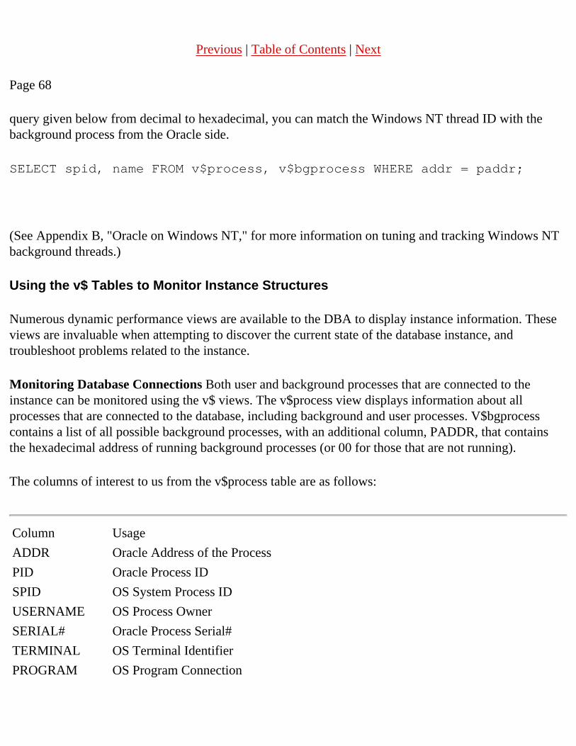
Previous | Table of Contents | Next
Page 68
query given below from decimal to hexadecimal, you can match the Windows NT thread ID with the background process from the Oracle side.
SELECT spid, name FROM v$process, v$bgprocess WHERE addr = paddr;
(See Appendix B, "Oracle on Windows NT," for more information on tuning and tracking Windows NT background threads.)
Using the v$ Tables to Monitor Instance Structures
Numerous dynamic performance views are available to the DBA to display instance information. These views are invaluable when attempting to discover the current state of the database instance, and troubleshoot problems related to the instance.
Monitoring Database Connections Both user and background processes that are connected to the instance can be monitored using the v$ views. The v$process view displays information about all processes that are connected to the database, including background and user processes. V$bgprocess contains a list of all possible background processes, with an additional column, PADDR, that contains the hexadecimal address of running background processes (or 00 for those that are not running).
The columns of interest to us from the v$process table are as follows:
Column Usage
ADDR Oracle Address of the Process
PID Oracle Process ID
SPID OS System Process ID
USERNAME OS Process Owner
SERIAL# Oracle Process Serial#
TERMINAL OS Terminal Identifier
PROGRAM OS Program Connection

BACKGROUND 1 for Background Process, NULL for User Process
The columns of interest to us from the v$bgprocess table are as follows:
Column Usage
PADDR Oracle Process Address (Same as ADDR column of v$process)
NAME Name of the Background Process
DESCRIPTION Description of the Background Process
ERROR Error State Code (0 for no error)
You can display the addresses and names of all running background processes by joining the v$process and v$bgprocess table, as in the following query:
Page 69
SELECT spid, nameFROM v$process, v$bgprocessWHERE paddr(+) = addr;
Information about user sessions that are connected to the database are stored in the v$session view. The v$session view contains many fields, and a great deal of valuable information can be accessed from this view.
The columns of interest from the v$session view are as follows:
Column Usage
SID Session Identifier
SERIAL# Session Serial#
PADDR Address of Parent Session
USER# Oracle User Identifier (from the SYS.USER$ table)
USERNAME Oracle Username

COMMAND
Current Command in Progress for this Session. For number to command translations, see the sys.audit_actions table
STATUS Status of the Session (ACTIVE, INACTIVE, KILLED)
SERVER
Type of Server Connection the Session Has DEDICATED, SHARED, PSEDUO, or NONE)
OSUSER OS Username the Connection Has Been Made From
PROGRAM OS Program Making the Connection into the Database
TERMINAL Type of Terminal the Connection Is Made From
TYPE Type of Session (BACKGROUND or USER)
SQL_HASH_VALUE and SQL_ADDRESS
Used to Uniquely Identify the Currently Executing SQL Statement
The following query displays important information on connected processes. It also demonstrates the manner in which the process views relate to each other:
col bgproc format a6 heading `BGProc'col action format a10 heading `DB Action'col program format a10col username format a8col terminal format a10
Page 70
SELECT b.name bgproc, p.spid, s.sid, p.serial#, s.osuser, s.username, s.terminal,

DECODE(a.name, `UNKNOWN', `-----', a.name) actionFROM v$process p, v$session s, v$bgprocess b, sys.audit_actions aWHERE p.addr=s.paddr(+) AND b.paddr(+) = s.paddr AND a.action = NVL(s.action, 0)ORDER BY sid;
By querying the v$access view, you can display information on what database objects users are currently accessing. This is useful when trying to figure out what a third-party application or undocumented procedure is doing, and can also be used to resolve security problems. By using a DBA account to run an application or procedure that is giving you security problems, you can determine the exact objects to which security should be granted.
Finally, the v$mts view contains tracking information for shared server processes. This view contains columns for maximum connections, servers started, servers terminated, and servers highwater.
Monitoring the Shared SQL Area Often it is useful to be able to look into the RDBMS engine and see what SQL statements are being executed. The v$sqlarea view contains information on SQL statements in the shared SQL area, including the text of SQL statements executed, the number of users accessing the statements, disk blocks and memory blocks accessed while executing the statement, and other information.
NOTE
The disk_reads and buffer_gets columns that are found in v$sqlarea track the number of blocks that are read from disk and from the buffer cache. These two columns are quick and easy ways to find queries that are utilizing large amounts of database resources.
The v$open_cursor view is also useful to investigate cursors that have not yet been closed. The following query displays all open cursors for a given user's SID:
SELECT b.piece, a.sql_textFROM v$open_cursor a, v$sqltext bWHERE a.sid = &SID and a.address = b.address and a.hash_value = b.hash_valueORDER BY b.address, b.hash_value, b.piece asc;

The v$sqltext view can also be used to determine what SQL statements are passed to the database engine. Unlike v$sqlarea, which only stores the first 80 characters of the SQL statement, this view holds the entire SQL statement. The v$sqltext_with_newlines view is identical to
Page 71
NOTE
v$sqltext, except that the newline characters in the SQL statements have been left in place.
The SQL statements stored in v$sqltext are split into pieces. To retrieve the entire statement, you have to retrieve all the parts of the SQL statement and order by the PIECE column.
Monitoring the SGA There are two v$ views available that provide information about the operation of the SGA. The v$sga view displays the size (in bytes) of each major component of the SGA, including the redo log cache, the database buffer cache, and the shared pool. The v$sgastat contains much more interesting information. Within this view you find the specific size for each individual memory structure contained in the SGA, including the memory set aside for stack space and PL/SQL variables and stacks. You can also query this view to find the amount of free memory available in the SGA:
SELECT bytes FROM v$sgastat WHERE name = `free memory';
Monitoring the Library and Dictionary Cache Two views exist that contain information regarding the library and data dictionary cache. v$librarycache contains library cache performance information for each type of object in the library cache. The v$rowcache view contains performance information for the data dictionary cache. (See Chapter 31 for more information on these views and the information contained in them.)
Monitoring the Parallel Query Processes The v$pq_sysstat and v$pq_tqstat views contain information on the parallel server processes and their behavior. Query v$pq_sysstat to display current runtime information on parallel query servers, such as the number of query servers busy and idle and dynamic server creation and termination statistics. The v$pq_tqstat view contains information on queries that have previously run that used parallel query servers. (See Chapter 26, "Parallel Query Management," for more information on tracking the parallel servers.)
Monitoring the Archiver Processes Archiver activity is stored in the v$archive view. You can retrieve information on the archived logs written by ARCH from this view. (For an explanation of the columns in this view, see Chapter 27.)

Monitoring the Multi-Threaded Server Processes The v$mts, v$dispatcher, and v$shared_server views contain information on the status of the MTS processes and memory structures. v$mts contains tracking information on the shared server processes such as the number of servers started, terminated, and the highwater value for running servers. v$dispatcher contains information on the dispatcher processes running. From this view you can query the name, supported protocol, number of bytes processed, number of messages processed, current status, and other runtime information relating to the dispatcher processes. The v$shared_server view provides the same type of information, but for the shared running shared server processes.
(See Chapter 19, "Oracle Networking Fundamentals," for more information on setting up and tuning the shared server and dispatcher processes.)
Previous | Table of Contents | Next

Previous | Table of Contents | Next
Page 77
Parameter Name Use
log_archive_start
Enables or disables automatic archiving. When true, the ARCH process will automatically start when the instance is started.
log_buffer Number of bytes allocated to the redo log buffer.
log_checkpoint_interval The number of redo log file blocks that must be filled to trigger a checkpoint.
max_dump_file_size Maximum size in operating system blocks of Oracle trace files.
processes
Maximum number of OS processes that can connect to the database, including the background processes. Important when tuning shared memory on a UNIX server.
remote_login_passwordfile
Specifies whether a password file is used for remote internal authentication, and how many databases can use a single password file. Can be set to NONE, SHARED, and EXCLUSIVE.
rollback_segments List of rollback segments to automatically take online at database startup.
sequence_cache_entries
Number of sequences that can be cached in the SGA. Should be set to the maximum number of sequences that will be used in the instance at one time.

shared_pool_size Size of the shared pool, in bytes.
snapshot_refresh_processes
Number of SNP processes to start at instance startup. SNP processes are responsible for refreshing snapshots and running database jobs submitted with DBMS_JOB.
timed_statistics
Enables or disables the collecting of timing statistics for the database. While setting this to true incurs a minimal performance overhead, it allows much greater flexibility in database tuning.
user_dump_dest
Destination directory for user trace files,including those generated by setting sql_trace to true.
The Control FileThe control file is the heart of the database. It contains information on what datafiles and redo log files belong to the database, what character set the data should be stored as in the database, the status and revision of each datafile in the database, and other critical information. Most of the parameters contained in the control file are set during database creation and are relatively static—they do not change from day to day. The control file is in binary format and cannot be read or edited manually.
Page 78
The control file is created when the database is created. Most databases operate with multiplexed control files (as explained later) and are therefore usually referred to in the plural. The specific control files created are those specified in the CONTROL_FILES init.ora parameter. The database creation parameters specified in the CREATE DATABASE clause are stored in these files.
The database cannot be opened without the correct control files. If the control file is unavailable or corrupted for some reason, the database cannot be started and the data contained in the database cannot be accessed. For this reason, mirroring of the control files is internally supported by the Oracle server and is highly recommended. To mirror control files in a new database, merely specify more than one value for the CONTROL_FILES init.ora parameter before issuing the CREATE DATABASE command. To mirror control files in a preexisting database, you must shut down the database, copy the current control file to the directories where you want it to be mirrored, edit the CONTROL_FILES parameter to specify the new control file locations, and start the database.

NOTE
A good rule of thumb is to store no fewer than three copies of the control files on three separate physical disks.
Unfortunately, modifying control file parameters is not as easy as changing an initialization parameter and bouncing the database. To change any of the control file parameters, you must re-create the control files. Follow these steps to re-create your control file:
1. Back up your database. Making an error while modifying your control file can corrupt your database beyond recovery. Never perform this activity without a valid backup of the database.
2. Issue the ALTER DATABASE BACKUP CONTROLFILE TO TRACE; command from Server Manager or SQL*Plus. This creates a user trace file (located in USER_DUMP_DEST) with the commands necessary to re-create your current control file.
3. Edit the trace file generated in the preceding step. Delete all of the lines in the trace file except for the CREATE CONTROLFILE statement. Set the new parameter values.
4. Shut down your database normal, by issuing the SHUTDOWN command in Server Manager. 5. Start your database in nomount mode, by issuing the STARTUP NOMOUNT command from
Server Manager. 6. Execute ALTER DATABASE OPEN;.
You can avoid ever having to re-create your control files by setting the database parameters during database creation to values higher than you'll ever need. The only thing wasted in setting these control file parameters higher than needed is a negligible amount of disk space.
Page 79
CAUTION
It's important that you set the CHARACTERSET parameter correctly when you create the database. Changing this parameter requires re-creating the entire database. It cannot be changed by rebuilding the control file.
The configurable control file parameters are listed in Table 6.2.
Table 6.2 Modifiable Configuration Parameters Contained in the Control File
Parameter Name Description

MAXLOGFILES Maximum number of online redo log files
MAXLOGMEMBERS Maximum number of members per redo log file
MAXDATAFILES Maximum number of datafiles
MAXINSTANCES Maximum number of instances that can mount this database(parallel server)
MAXLOGHISTORY Maximum number of archived redo log file groups to use forinstance recovery (parallel server)
NOTE
To change the database name, re-create the control file as described, but change the REUSE DATABASE "OLD_NAME" line in the trace file to SET DATABASE "NEW_NAME".
The V$CONTROLFILE view lists the control files that the Oracle server is currently reading from and writing to.
Online Redo Log FilesThe log writer background process (LGWR) writes the contents of the redo log cache to the online redo log files. The redo logs store all of the change information for the database and are used by Oracle during database recovery.
As shown in Figure 6.1, the online redo log files are made up of at least two groups of redo log files and are written to in a circular nature. A redo log group is active if it is currently being written to by LGWR. A log switch occurs when the current log group fills up and LGWR stops writing to it and moves on to the next one. When a log switch occurs and archivelog mode is enabled for the database, the redo log group previously written to is locked by the archiver (ARCH) process and copied to disk or tape, depending on your configuration. If LGWR catches up with the ARCH process and needs to write to the group currently being written to by ARCH, all database activity will be suspended until ARCH finishes writing to the log. If you see errors in your alert.log file stating that a free log group could not be latched by LGWR, this behavior is occurring in your database, indicating that you need to add more redo log groups or adjust the size of the groups.
Previous | Table of Contents | Next

Previous | Table of Contents | Next
Page 80
FIG. 6.1Redo log groups withmultiple members.
Each log group can consist of multiple members. Each member of a log group is an exact mirror of the others, and redo log entries are written to each member in parallel. If LGWR cannot write to a member of the group, it does not fail. Rather, it writes an entry into the alert.log file. By using multiple members per group, you can safeguard against database failure resulting from lost redo logs. As long as one member of the group is accessible, the database will continue to function.
NOTE
The same functionality can be obtained by mirroring your redo log groups using RAID 1 (Mirrored) or RAID 5 volumes. This alleviates the overhead caused when LGWR has to update multiple log group members for each database transaction.
As shown in Figure 6.2, the redo logs are written to in a circular fashion. LGWR writes to one group until it is full. It then moves on to the next group in the sequence. Meanwhile, ARCH will copy the just-filled online redo log to the operation system as an archived redo log. This process will continue until all of the logs have been filled, and then LGWR will begin writing back at the first online redo log. At no point will LGWR write to an online redo log that ARCH is still copying. If this happens, all database activity will seem to halt until ARCH has finished its copy. This LGWR-ARCH contention can be avoided by having online redo log groups of ample size and number available in the database.
Page 81
FIG. 6.2Redo logs are written toin a circular fashion.

The V$LOG and V$LOGFILE views hold information on the online redo log files. The following query checks the status of the current logs:
SELECT member, bytes, members, a.statusFROM v$log a, v$logfile bWHERE a.group# = b.group#ORDER BY member;
SELECT b.member, b.bytes, b.members, a.statusFROM v$log a, v$logfile bWHERE a.group# = b.group#ORDER BY b.member;
The Trace File(s)All Oracle databases have at least one file where system messages, errors, and major events are logged. This file, named sidALRT.log (where sid is the system identifier for the database), is stored at the location specified by the init.ora parameter BACKGROUND_DUMP_DEST. It is the first place you should look when investigating database problems. Critical failures are always logged here, as well as database startup and shutdown messages, log switch messages, and other events.
Background and user processes also create their own trace files where problems and failures are logged. Background process trace files are stored in the BACKGROUND_DUMP_DEST location, while user trace files are stored in the directory pointed to by the USER_DUMP_DEST parameter setting. Setting the USER_DUMP_DEST directory differently than that pointed to by BACKGROUND_DUMP_DEST will allow you to keep track of the different classes of trace files. Background process trace files are named sidPROC.trc, where sid is the system identifier for the database and PROC is the name of the background process (DBWR, LGWR, SMON, PMON, and so on).
User session trace files are given an ora prefix, followed by a sequence of unique numbers, with a .trc file extension. User session trace files are generated when a user session causes an unrecoverable problem (such as a deadlock or a crashed server process) or when the user session is explicitly told to, such as when SQL tracing is enabled or an ALTER DATABASE BACKUP CONTROLFILE TO TRACE command is issued. To enable SQL tracing, issue ALTER SESSION
Page 82
SET SQL_TRACE=TRUE from the SQL*Plus prompt, or set the SQL_TRACE init.ora parameter to true. Be cautious, however, because setting SQL_TRACE to true in init.ora will cause all SQL statements that occur against the database to be written to trace files; this will generate an enormous amount of trace information.

The current settings for the BACKGROUND_DUMP_DEST and USER_DUMP_DEST parameters can be queried from the V$PARAMETER view.
The ROWIDFor the Oracle database to retrieve information, it must be able to uniquely identify each row in the database. The internal structure the Oracle RDBMS uses for this task is called the ROWID, a two-byte value that stores the physical location for a row in the database. The format of the ROWID is as follows:
BBBBBBBB.RRRR.FFFF
where
BBBBBBBB is the block number (in hex) where the row resides in the datafile,
RRRR is the row number (in hex) in the block where the data row exists, and
FFFF is the file where the block exists.
For example, a row in a table might have a OWID as follows:
0000068C.0000.0001
This ROWID is in the first datafile (0001), the 68C (hex) block in that datafile, and the first row in that block (0000).
NOTE
You can match the file number from the preceding ROWID to the filename by querying the DBA_DATA_FILES view. In Oracle7, these file numbers are fixed, while in Oracle8 they are determined at database startup.
A row is assigned a ROWID when it is first created. The ROWID remains the same until the row is deleted or the segment the row is in is reorganized (through import/export, third party reorganization tools, and so on). Using the ROWID is the fastest method of finding a row in the database. Every table

in the database contains a pseudocolumn named ROWID, which can be queried to show the ROWID of each row in the table.
Because of the unique nature of the ROWID, it can be used to creatively solve many different problems. For example, one of the most common usages of the ROWID is to identify columns with duplicate values in the database. The following SQL script shows how this can be done:
delete from duplicate_tablewhere ROWID not in (select MIN (ROWID) from duplicate_table group by a1, a2);
You can also use the value of the actual ROWIDs in queries. The following SQL script will display the number of database files a table has rows in:
SELECT COUNT(DISTINCT(SUBSTR(ROWID, 15, 14)))) "Files"FROM test_table;
Previous | Table of Contents | Next

Previous | Table of Contents | Next
Page 93
CHAPTER 7
Exploring the Oracle Environment
In this chapter
● Creating the Oracle Environment 94 ● Designing an Optimal Flexible Architecture 94 ● Configuring the Oracle Environment 101 ● Understanding the Oracle Software Environment 101 ● Creating Your First Database 106 ● Exploring the Oracle Database 111 ● Exploring an Unfamiliar Environment 115
Page 94
Creating the Oracle Environment
The Oracle database is a powerful yet complicated data storage and retrieval system, capable of supporting enormous workloads while maintaining high levels of performance, security, and data integrity. An integral part of a successful database is the manner in which the software is installed and configured on the database server. This chapter examines the role the server software and configuration plays in the database environment, and deciphers the sometimes confusing aspects of the Oracle server installation. This chapter also explores strategies for creating your Oracle server environment, as well as your first Oracle database. Finally, it looks at what you can do to familiarize yourself with an unfamiliar Oracle database.
When configuring a server to house the Oracle software, you must take several key factors +into consideration. These include the flexibility of the design, the ease of administration, and the simplicity of the structure. If you design your environment with these points in mind, you will be rewarded with an environment conducive to your uptime and performance goals, as well as avoid the problems and anxiety that a poorly designed server structure can create.
Designing an Optimal Flexible Architecture

The Oracle standard for creating and configuring your Oracle environment is named the Optimal Flexible Architecture, or OFA, Standard. It is a set of rules and guidelines that enables you to easily create and configure a production-level Oracle server. As the name states, the OFA Standard was created to give you the most flexible Oracle environment without sacrificing usability, ease of administration, or simplicity of design.
Mr. Cary Millsap of Oracle Corporation wrote the OFA Standard in the early 1990s. The definitive white paper on the structure can be found at http://www.europa.com/~orapub/index.html. Mr. Millsap's article goes into much more detail than will be described here. His white paper deals with configuring the entire environment, while we are concerned with the creation and configuration of the operating system directory structures and naming conventions used to support the Oracle database. Mr. Millsap's OFA Standard paper is required reading for any Oracle DBA or systems integrator interested in the best practices for implementing an Oracle installation.
Mr. Millsap sums up the purpose of the OFA Standard Recommendations with his statement that "A good standard should act as a strong floor, without becoming a ceiling that inhibits `creative magic.'" The OFA Standard Recommendations are just those—recommendations. Your specific environment will have requirements and specifications that are best met with methods not included in (or contrary to) the OFA Standard. However, close study of the OFA Standard will reveal many best practice methods that would only be obvious through difficult trial, error, and experience.
Creating Top-Level Directories
The first step in configuring your environment is to decide on the naming and creation of the OS mount points and top-level directories of your Oracle installation. As with many
Page 95
configuration items, the implementation varies from UNIX to Windows NT, but the general concepts remain the same. The first OFA rule relates to this topic and is
OFA Recommendation 1: Name all mount points that will hold site-specific data to match the pattern /pm, where p is a string constant chosen not to misrepresent the contents of any mount point, and m is a unique fixed-length key that distinguishes one mount point from another.
In other words, create top-level mount points that are unique, but do not have meaning in and of themselves. The character portion (p) should be short and simple—one or two characters are ideal. The numbered portion distinguishes the mount points from each other. Each mount point should have the same named portion, and be of the same length, for example, u01, u02, and u03 or ora01, ora02, and ora03.

On a Windows NT server, the different drives and volumes are already separated according to drive letters. This makes the usage of mount-point names as described above unnecessary. Use a directory named orant (the default Oracle name) on each drive to denote Oracle applications and files.
NOTE
To minimize confusion, UNIX naming conventions will be used throughout this explanation. However, unless otherwise indicated, all of the structure and naming conventions given are applicable to both UNIX and Windows NT environments.
Using mount points without site-specific, application-specific, or hardware-specific connotations enables great flexibility when reconfiguring your system. Consider the following example: Bob, a novice DBA, names mount points on his UNIX system that refer to the physical disks each mount-point volume is attached to. This makes it very easy for Bob to balance his datafile I/O over drives. By glancing at the pathname, he can tell that his main data tablespace is on DISK01, while his index tablespace is on DISK05. But, as always happens, Bob's database grows, forcing him to add more disks and new hardware. Bob wants to take advantage of his new RAID controller to stripe and mirror some volumes, which means he must reorganize his entire drive subsystem to accomplish this goal. Unfortunately, this also means that if he wants to keep his naming convention, he must rename his mount points and change all of his backup scripts, applications, and so on, to point to the new paths. Bob could have avoided this hassle by using directory names that are unique, but that by themselves have no meaning.
Using Application Directories
One of the benefits gained from implementing an OFA-compliant configuration is the ease in which multiple applications and multiple versions of the same application can be installed, using the same directory structure. In an OFA environment, each application has its own home directory that stores the binaries, configuration files, and so forth that are necessary for running the application. The next two OFA rules relate to this and are as follows:
OFA Rule 2: Name application home directories matching the pattern /pm/h/u, where pm is a mount-point name, h is selected from a small set of standard directory names, and u is the name of the application or application owner.
Previous | Table of Contents | Next

Previous | Table of Contents | Next
Page 91
information, while not showing Social Security number and salary data), and to make complicated queries easier to understand and use. Views can also be used to hide distributed database objects by creating views on remote database tables. Any statement that can be executed as a SQL query can be created as a view.
NOTE
Views can be very helpful when designing applications because they can be used to hide complicated query logic in a table format that is much easier to query. They can be created with optimizer hints embedded in them, to ensure top query performance.
The DBA_VIEWS view holds information on views created in the database.
Sequences
Sequences are database objects that are used to generate unique numbers. A sequence is created with a starting value, an increment, and a maximum value. Each time a number is recalled from a sequence, the current sequence value is incremented by one. Each sequence-generated number can be up to 38 digits long.
You use a sequence by selecting the NEXTVAL or CURRVAL pseudocolumns from it. If you have a sequence named EMP_SEQ, for example, issuing SELECT EMP_SEQ.NEXTVAL FROM DUAL will return the next integer value of the sequence and increment the current value of the sequence by one. You can SELECT EMP_SEQ.CURRVAL FROM DUAL to return the current integer value of the sequence. Note that to use CURRVAL, you must have initialized the sequence for your user session by previously issuing a query on the NEXTVAL pseudocolumn of the sequence.
The most common usage of sequences is to provide unique numbers for primary key columns of tables. Information on sequences is stored in the DBA_SEQUENCES view.
Triggers
Triggers are stored procedures that fire when certain actions occur against a table. Triggers can be coded to fire for inserts, updates, or deletes against a table and can also occur for each row that is affected or for each statement. Triggers are most often used to enforce data integrity constraints and business rules that are too complicated for the built-in Oracle referential integrity constraints. Information on database

triggers can be found in the DBA_TRIGGERS view.
Synonyms
Synonyms are database pointers to other database tables. When you create a synonym, you specify a synonym name and the object the synonym references. When you reference the synonym name, the Oracle server automatically replaces the synonym name with the name of the object for which the synonym is defined.
There are two types of synonyms: private and public. Private synonyms are created in a specific schema and are only accessible by the schema that owns it. Public synonyms are owned by the PUBLIC schema, and all database schemas can reference them.
Page 92
It's important to understand the order in which an object name is resolved within a SQL statement. If the SQL statement SELECT * FROM EMP_SALARY is issued, the Oracle server attempts to resolve the EMP_SALARY object in the following way:
1. First, the server checks to see if a table or view named EMP_SALARY exists in the issuing user's schema.
2. If the table or view doesn't exist, Oracle checks for the existence of a private synonym named EMP_SALARY.
3. If this private synonym exists, the object that the synonym references is substituted for EMP_SALARY.
4. If the private synonym does not exist, the existence of a public synonym named EMP_SALARY is checked.
5. If a public synonym does not exist, Oracle returns the message ORA-00942, table or view does not exist.
Public synonyms should be used with care. Because all schemas can use public synonyms to resolve object names, unpredictable results can occur.
Information on public synonyms is stored in DBA_SYNONYMS. Note that the owner of public synonyms will be listed as PUBLIC in this view.
Database Links
Database links are stored definitions of connections to remote databases. They are used to query remote tables in a distributed database environment. Because they are stored in the Oracle database, they fall under the category of database object. More information on database links can be found in Chapter 28, "Distributed Database Management."

Information on database links can be found in the DBA_DB_LINKS data dictionary view.
CAUTION
DBA_DB_LINKS is one of the views that can store passwords in clear text, if the database link is defined with a specific UserID and password to connect to the remote database. Care should be taken when allowing end users access to this database view.
Packages, Procedures, and Functions
Stored packages, procedures, and functions are stored in the data dictionary, along with their source code. A stored procedure is a code unit that does work, can be passed arguments, and can return values. A stored function is a code unit that is passed an argument and returns one value. A package is a collection of procedures, variables, and functions, logically grouped by function. See Chapter 10, "PL/SQL Fundamentals," for more information.
You can access information on stored packages, procedures and functions through the DBA_OBJECTS and DBA_SOURCE views.
Previous | Table of Contents | Next

Previous | Table of Contents | Next
Page 88
the buffer cache. If another user session requests the same data, the before image stored in the rollback segment is returned (this is called a consistent read). When the session that is making the change commits, the rollback segment entry is marked invalid.
Multiple user sessions can share a single rollback segment. Each rollback segment is made up of at least two extents. When a transaction starts, the user session gets an exclusive lock on an available extent in an available rollback segment. Transaction information is then written to the rollback segment. If the transaction fills the first extent, it allocates another extent. If another extent is unavailable, the rollback segment automatically allocates another extent to itself, which the user session grabs. This is called rollback segment extension. Because extent allocation affects performance, your goal should be to enable all transactions to run without allocating new extents.
If the rollback segment is unable to allocate another extent (either because the maximum number of extents has been reached for the rollback segment or there are no more free extents in the rollback segment tablespace), an error occurs and the transaction is rolled back. This commonly occurs in large data loads, where online rollback segments do not provide sufficient space to store all of the rollback information for the transaction.
See Chapter 21 for more information on creating and administering rollback segments.
The DBA_ROLLBACK_SEGS view contains information on rollback segments.
Table Clusters
A table cluster is a database object that physically groups tables that are often used together within the same data blocks. The clustering of tables is most effective when you're dealing with tables that are often joined together in queries. A table cluster stores the cluster key (the column used to join the tables together), as well as the values of the columns in the clustered tables. Because the tables in the cluster are stored together in the same database blocks, I/O is reduced when working with the clusters.
Hash Clusters
Hash clusters are the final option for database storage. In a hash cluster, tables are organized based upon a hash value derived by applying the hash function to the primary key values of the tables. To retrieve data from the hash cluster, the hash function is applied to the key value requested. The resulting hash value gives Oracle the block in the hash cluster where the data is stored.

Using hash clusters can significantly reduce the I/O required to retrieve rows from a table. There are several drawbacks to using hash clusters, however. See Chapter 21 for more information on creating and administering hash clusters.
Page 89
Using the Oracle Data Dictionary
The data dictionary is the repository of information on all of the objects stored in the database. It is used by the Oracle RDBMS to retrieve object and security information and by the end-users and DBAs to look up database information. It holds information on the database objects and segments in the database, such as tables, views, indexes, packages, and procedures. The data dictionary is read only; you should NEVER attempt to manually update or change any of the information in any of the data dictionary tables. It consists of four parts: the internal RDBMS (X$) tables, the data dictionary tables, the dynamic performance (V$) views, and the data dictionary views.
Internal RDBMS (X$) Tables
At the heart of the Oracle database are the so-called internal RDBMS (X$) tables—the tables used by the Oracle RDBMS to keep track of internal database information. The X$ tables are cryptically named, undocumented, and nearly impossible to decipher. Most of them are not designed to be used directly by the DBAs or end users. Nonetheless, they contain valuable information. Many undocumented or internal statistics and configurations can be found only in the X$ tables.
The easiest way to decipher what is stored in a particular X$ table is to work backward from a known data dictionary table. The SQL*Plus autotrace feature is invaluable for this work. For example, to determine where the information in V$SGASTAT is really stored, you can perform the following analysis:
● Log in to SQL*Plus as SYS (or an account with explicit access to the X$ and V$ tables). If a plan_table does not exist for the schema you are logged in to, create one by running $ORACLE_HOME/rdbms/admin/UTLXPLAN.sql.
● Issue the following SQL*Plus command: SET AUTOTRACE ON. ● Issue a query against the table whose components you are interested in. Set the WHERE clause to
a value that will never be true, so that no rows are returned: SELECT * FROM v$sgastat WHERE 0 =1;.
● Among other information, the autotrace will return output similar to the following: Execution Plan
0 SELECT STATEMENT Optimizer=CHOOSE
1 0 FILTER

2 1 FIXED TABLE (FULL) OF `X$KSMSS'
From the output of the SQL trace, you can decipher the data dictionary base tables from which the information for the view is extracted. Querying the X$ tables found in this manner often produces surprising information.
Page 90
Data Dictionary Tables
The data dictionary tables hold information for tables, indexes, constraints, and all other database constructs. They are owned by SYS and are created by running the SQL.BSQ script (which happens automatically during database creation). They are easily identified by the trailing dollar sign at the end of their names (tab$, seg$, cons$, and so on). Most of the information found in the data dictionary tables can be found in the data dictionary views, but certain applications and queries still benefit from using the information contained in the base tables.
The columns and tables of the data dictionary are well documented in the SQL.BSQ file. This file is found in the $ORACLE_HOME/dbs directory. By familiarizing yourself with the contents of SQL.BSQ, you can gain a better understanding of how the Oracle RDBMS actually stores the data dictionary and database information.
Dynamic Performance (V$) Views
The dynamic performance (V$) views are the mainstay of the Oracle DBA. These views contain runtime performance and statistic information on a large number of database functions. They are also fairly readable (as opposed to the X$ tables) and are meant to be used by the DBA to diagnose and troubleshoot problems. Documentation on most V$ views can be found in the Oracle Reference Manual, supplied on your Oracle server media.
Note that the V$ views are actually public synonyms to the V_$ views, owned by SYS. This is important to note when writing stored procedures or functions that read the V$ tables. It is often necessary to reference or grant privileges to the base V_$ view rather than the V$ public synonym.
Data Dictionary Views
The data dictionary views are views created on the X$ and data dictionary tables and are meant to be queried and used by end users and DBAs. They are divided into three categories—the DBA_, ALL_, and USER_ views. The DBA_ views contain information on all objects in the database. For example, DBA_TABLES contains information on all tables created. The ALL_ views contain information on all objects to which the user querying the table has access. The USER_ views contain information on all

objects the user querying the table owns.
Other Database Objects
There are several other objects stored in the database that are not rightfully classified as segments but should be discussed nonetheless. They include views, sequences, synonyms, triggers, database links, and stored packages, procedures and functions. They are described in the following sections.
Views
Views are stored SQL statements that can be queried. A view is used for security reasons to hide certain data (such as an HR view that shows only first name, last name, and address
Previous | Table of Contents | Next

Previous | Table of Contents | Next
Page 96
OFA Rule 3: Store each version of Oracle server distribution software in a directory matching the pattern h/product/v, where h is the application home directory of the Oracle software owner and v represents the version of the software.
A sample implementation of this rule is given in the following directory template:
/[mount_point]/APP/[application_name]/PRODUCT/[version]/application home
In this example, we see that application home directories are stored in the APP subdirectory directly underneath our mount point. We next use a generic name to identify the directory under which the application will be stored. The PRODUCT directory and version then follow.
A sample hierarchy using this naming convention is
/u01
app finance [...] qse [...]
oracle
admin
product
7.1.6
[...]
7.3.3
[...]

8.0.3
[...]
While this method may seem more complicated than necessary, the resulting flexibility and ease of administration is well worth it. As you can see, under this mount point you have three applications installed—finance, QSE, and Oracle. Finance and QSE are third-party or homegrown applications, and the directory structures underneath the main directories follow the same format as shown in the Oracle hierarchy. In the Oracle application directory, you see the product and admin subdirectories. Within the product subdirectory are three versions of the Oracle software—7.1.6, 7.3.3, and 8.0.3. Any change or new installation of Oracle software can be made to one version without fear of interaction with any other version.
Separating the versions in this manner is very important when performing testing and cutover of new Oracle versions. Obviously you need the ability to easily install a new version of the software without impacting your production installation. After your new version is tested, cutover to the new version is a simple matter of setting the correct environment variables to the new directory. The old version then can be deleted at your leisure.
Managing Database Files
One of the needs that necessitated the creation of the OFA guidelines was the difficulty DBAs faced when simultaneously administering many databases. A method to organize administrative information and data into a manageable and predictable format was needed. The admin directory we saw earlier is used to store files related to administering the database and goes a
Page 97
long way in improving the capability of a single person to keep track of many databases. Our next OFA rule is related to this structure:
OFA Rule 4: For each database with db_name=d, store database administration files in subdirectories of /h/admin/d, where h is the Oracle software owner's login home directory.
The following chart shows a sample admin directory structure:
/u01/app/oracle/admin PROD

bdump udump cdump pfile sql create
The subdirectories in the admin directory are explained in Table 7.1.
Table 7.1 ADMIN Directories
Directory Name
Usage
bdump Background dump files (value of BACKGROUND_DUMP_DEST)
udump User dump files (value of USER_DUMP_DEST)
cdump Core files (UNIX only)
pfile init.ora and any other database initialization parameters
sql Database administration SQL files
create Scripts used to create the initial database and database objects
init.ora files, trace and dump files, alert.log, and so forth are all stored in this central administrative directory. This eases administering the large amounts of data produced by an Oracle database. You can add directories to store other data as the need arises.
NOTE
On UNIX platforms, create a link of the init.ora file from the $ORACLE_HOME/dbs directory to the admin/pfile directory. This ensures the Oracle default configuration is intact, while allowing you to benefit from the OFA structure. On Windows NT platforms, you will have to either specify the full pathname to the init.ora file when starting the database and create an OFA- compliant structure or store the init.ora files in the default $ORACLE_HOME/database directory to keep the default Oracle configuration intact.
Page 98

Naming Conventions
When managing multiple databases on one database server, a file-naming convention is important. The OFA standard gives the following rule for naming database files:
OFA Rule 5: Name Oracle database files using the following patterns:
/pm/q/d/control.ctl _ control files
/pm/q/d/redon.log _ redo log files
/pm/q/d/tn.dbf _ data files
where:
1 pm is a mount-point name1 q is a string denoting the separation of Oracle data from all other files1 d is the db_name of the database1 n is a distinguishing key that is fixed-length for a given file type1 t is an Oracle tablespace name
Never store any file other than a control, redo log, or data file associated with a database d in /pm/q/d.
Deviation from this standard depends on your personal preference, but the naming convention ideas should not be ignored. Use a meaningful filename extension, include the tablespace name in datafile names, and keep all datafiles in their own exclusive directories.
A template for an alternative naming standard that keeps the original naming conventions could be tn_SID_n.ext, where tn is an abbreviation for the tablespace the datafile is for, SID is the database the datafile belongs to, and n is the datafile number.
Try to keep the tablespace abbreviation brief and, if possible, keep it a set number of letters. This will produce uniform reports. Also, the number portion for redo log files should indicate both the log group and member—using a combination of numbers and characters, such as 01a (first log group, first member) and 02c (second log group, third member), works well. Names using the alternative notation are shown in Table 7.2.

Table 7.2 Database File Examples
File Name Explanation
syst_PROD_01.dbf First SYSTEM tablespace datafile for the PROD database
ctrl_TEST_02.ctl Second controlfile for the TEST database
redo_PPRD_01a.log
First member of first redo log group for database PPRD
redo_PPRD_02c.log
Third member of second redo log group for database PPRD
data_PROD_02.dbf Second data tablespace datafile for the PROD database
initTEST.ora Initialization parameter file for the TEST database
Previous | Table of Contents | Next

Previous | Table of Contents | Next
Page 99
As you can see, investing the extra time in implementing a naming convention for your database files results in names that have no guesswork involved. You can immediately determine their function by glancing at the name.
The OFA rule also dictates that database datafiles, redo log files, and control files should be stored in a dedicated directory off of the mount point. The following shows a directory structure that complies with this recommendation, containing data for four databases:
/u01 app oradata PROD [...]
PPRD
[...]
DEVL
[...]
TEST
[...]
All datafiles, log files, control files, and archived redo log files are stored in the directory under the oradata subdirectory. Each database has its own directory, and ONLY database files are stored in these directories.
Putting It All Together
A wise person once said that the great thing about standards is the variety from which to choose. This is especially apt when describing the OFA guidelines. There is no one perfect solution for creating an

Oracle server environment because no two environments are the same.
The following are sample OFA implementations on both UNIX and Windows NT. These are meant to give you ideas and get you started. You may find specific points that, when reworked, serve your particular needs better than those presented. Explanations of each section are also given.
UNIX Implementation
/ Root Directory u01 u01 Mount Point app Application Directory oracle Oracle Application Directory admin Administrative Directory PROD PROD Database Directory pfile Initialization Parameter Files bdump Background Dump Files udump User Dump Files cdump Core Files create Database Creation Scripts sql SQL Scripts PPRD PPRD Database Directory [...] Same Directory Structure as PROD TEST TEST Database Directory [...] Same Directory Structure as PROD product Application Files
Directory
Page 100
7.1.3 Version 7.1.3 Files [...] ORACLE_HOME for version 7.1.3

8.0.3 Version 8.0.3 Files [...] ORACLE_HOME for version 8.0.3 qse QSE Application Directory admin Administrative Directory [...] Directories for QSE Administration product Application Files Directory [...] QSE Versions and Files oradata Oracle Database Files Directory PROD PROD Database Files PPRD PPRD Database Files TEST TEST Database Files u02 u02 Mount Point oradata Oracle Database Files Directory PROD PROD Database Files PPRD PPRD Database Files TEST TEST Database Files[...]
Windows NT Implementation
C: Drive Designator oracle Oracle Software Directory home Oracle Home Directory [...] ORACLE_HOME Contents oradata Oracle Database Files PROD PROD Database Files Directory [...] PROD Database Files PPRD PPRD Database Files Directory [...] PPRD Database Files admin Oracle Administrative Directories PROD PROD Administrative Directory [...] Same Structure as UNIX PPRD PPRD Administrative Directory [...] Same Structure as UNIXD: Drive Designator

oracle Oracle Software Directory oradata Oracle Database Files PROD PROD Database Files Directory [...] PROD Database Files PPRD PPRD Database Files Directory [...] PPRD Database Files[...]
One of the crucial factors in making the OFA standards work is the separation of application and database files. The admin and oradata directories are created in order to keep all database- specific files separate from the Oracle software. This is necessary to fulfill one of the promises discussed earlier; the simple and transparent cutover to new software versions.
The final OFA rule from Mr. Millsap's paper we are going to discuss follows:
OFA Rule 6: Refer to explicit path names only in files designed specifically to store them, such as the UNIX /etc/passwd file and the Oracle oratab file; refer to group memberships only in /etc/group.
Page 101
If followed, this rule will help you avoid a common pitfall we all step into: creating an application "on the fly" that becomes a common tool used everyday, which breaks as soon as any system reconfiguration is performed. Avoid using hard-coded directory names in a shell script, batch file, or application program. When working with the Oracle tools, this is easier than it sounds—any directory or value you might need to work with is probably already implemented as an environment variable or registry key.
Configuring the Environment
The Oracle server is a complex set of interacting programs and processes. The software environment involved is likewise complicated and often difficult to understand. Various parameters exist to control the behavior of the Oracle programs, set the locations for configuration or shared files, define the language and character set to use, and a myriad other traits. On a UNIX machine, these parameters are stored as environment variables, which are usually loaded from the supplied coraenv or oraenv files called from the user's login script. On a 16-bit Windows computer, the parameters are stored in the oracle.ini file. On 32-bit Windows computers (Windows 95, Windows NT, and so on), these configuration parameters are stored in the Registry.
The environment variable files or Registry keys are created the first time an Oracle product is installed on a machine. Subsequent software installations add to and update these configurations. Systems programmers or DBAs also modify these configurations by hand to tune, troubleshoot, and customize

the Oracle environment. A full description of the software configuration parameters can be found in your operating system-specific Oracle documentation. You should take a few minutes to familiarize yourself with the various parameters for your operating system— many problems can be solved with careful tweaking of these parameters.
NOTE
Don't confuse the Oracle configuration parameters with the initialization parameters of a database. The Oracle configuration parameters apply to the Oracle software installed on a computer, while the initialization parameters configure a single database.
There are several environment variables with which you should be immediately familiar, as they play an important role in the operation of the Oracle server. ORACLE_HOME defines the base path for the Oracle software. It is explained in detail later in this chapter. ORACLE_SID is set to the default database SID (System Identifier) for your session. Many tools use the ORACLE_SID to determine what database to connect to. It is important you always know what values these variables are set to—having wrong values for either of these can result in performing operations on the wrong database or using the wrong version of the Oracle tools.
Understanding the Oracle Software Environment
When you install the Oracle software on a server or client computer, an Oracle directory structure is created to store the binary executables, shared libraries, configuration files, trace files, and so on used by the Oracle programs. This directory tree is semi-standard across different server platforms and versions of Oracle software. Both server and client software is stored in the same directory.
Previous | Table of Contents | Next

Previous | Table of Contents | Next
Page 119
CHAPTER 8
SQL*Plus for Administrators
In this chapter
● Administering SQL*Plus 120 ● Using the SQL*Plus COPY Command 130 ● Using SQL to Create SQL 132 ● Restricting a User's Privileges in SQL*Plus 135 ● Tracing SQL Statements 139
Page 120
This chapter discusses SQL*Plus, Oracle's implementation of the Structured Query Language (SQL). SQL*Plus is an interactive program used to access an Oracle database. It is also the database administrator's best friend and an indispensable tool.
In addition to SQL*Plus, a database administrator (DBA) can interface with the database and use SQL*Plus commands (but only a subset of the commands) in two other tools:
● Server Manager ● Worksheet utility in the Enterprise Manager
Note that Server Manager replaces, beginning with Oracle7 7.3, the SQL*DBA utility that was used in Oracle version 6 and Oracle7 releases prior to 7.3.
Because SQL*Plus is such a vast subject, which cannot be dealt with in a single chapter, I will concentrate mainly on features of interest to DBAs, new features (EXECUTE and AUTOTRACE), and lesser-known and lesser-used features (COPY command, disabling commands).
Administering SQL*Plus
There are two files, glogin.sql and login.sql, that are used to administer SQL*Plus. The glogin.sql file is the global setup file, and login.sql is intended for individual use. These two files contain SQL*Plus

commands and/or SQL statements that are executed every time an Oracle user invokes SQL*Plus. The glogin.sql file is read and executed first, followed by the user's login.sql file.
The glogin.sql file is located in the $ORACLE_HOME/sqlplus/admin directory. The Oracle DBA may customize this file to include SQL*Plus commands, SQL statements, and PL/SQL blocks that will be executed by every SQL*Plus user at the beginning of his or her SQL*Plus session. The glogin.sql file is also known as a Site Profile.
NOTE
Under Windows 95/NT 4.0, the glogin.sql file is located in the directory %ORACLE_HOME%\PLUSnn, where nn represents the version of SQL*Plus installed on your machine. For example, if SQL*Plus 3.2 is installed, the directory name will be %ORACLE_HOME%\PLUS32.
Using SQL*Plus Environment Variables
There are two environment variables that are used by SQL*Plus:
● SQLPATH ● _editor
SQL*Plus uses the environment variable SQLPATH to identify the directory where the login.sql file is located. In other words, SQL*Plus will look in every directory defined in SQLPATH for login.sql, starting with the local directory—the directory you were in when you started SQL*Plus.
Page 121
For example, if you want SQL*Plus to look for login.sql first in the local directory, then in your home directory, and then in another directory, set SQLPATH as follows:
$ SQLPATH=".:$HOME:<other_directory>"; export SQLPATH --(Bourne/Korn shell)$ set SQLPATH=(. $HOME <other_directory>) -- C shell
Under Windows 95/NT 4.0, SQLPATH is defined in the Registry. The default value is $ORACLE_HOME\DBS (set during installation). The value for ORACLE_HOME is C:\ORAWIN95 for Windows 95 and C:\ORANT for Windows NT 4.0 (replace C: with the name of the disk drive where you installed Oracle, if you did not install it on your C: drive).
NOTE

Under Windows 95/NT 4.0, the login.sql file is located in directory %ORACLE_HOME%\DBS, the default value for SQLPATH.
To set or change the value of SQLPATH under Windows 95/NT 4.0, follow these steps:
1. Select Run from the Start menu. 2. Enter regedit.exe/regedit32.exe (for Windows 95/NT, respectively). 3. Click OK. 4. Double-click HKEY_LOCAL_MACHINE. 5. Double-click SOFTWARE. 6. Double-click ORACLE. 7. Double-click SQLPATH. 8. The Edit String dialog box appears. In the Value Data field, enter the new value for SQLPATH. 9. Click OK.
10. From the Registry menu, select Exit. 11. Reboot your machine for the new value to take effect (or log out and log back in
Windows NT 4.0).
NOTE
SQLPATH is also used by SQL*Plus to identify the location of SQL scripts that you run from SQL*Plus.
There is another environment variable that can be set in glogin.sql or login.sql. This environment variable is called _editor. It defines the editor you can use to edit SQL*Plus commands.
To set the value of _editor to the vi text editor, enter the following line in glogin.sql or login.sql:
define _editor=vi
If you use any other text editor, replace vi with the appropriate name. For more information on using different editors, see the section "Using Your Operating System Editor in SQL*Plus," later in this chapter.
Page 122
Invoking/Accessing SQL*Plus

To invoke SQL*Plus from the operating system prompt, use the following command:
$ sqlplus [[-S[ILENT]] [logon] [start]]|-?
The -S[ILENT]] parameter is used when running SQL*Plus from a shell script, because it suppresses all the information that SQL*Plus displays when invoked, such as the SQL*Plus banner, prompt messages, and the command prompt.
The [logon] section requires the following syntax:
username[/password] [@connect_string]|/|/NOLOG
The [start]] clause enables you to start SQL*Plus and run a command file containing any combination of SQL*Plus commands, SQL statements, and/or PL/SQL blocks. In addition, you can pass arguments to the command file. The start clause requires the following syntax:
@file_name[.ext] [arg...]
If you do not enter the username or the password, SQL*Plus prompts you to enter them.
After you successfully access SQL*Plus, you can enter three type of commands at the SQL*Plus prompt (SQL >):
● SQL commands/statements for working with database objects and manipulating the data stored in the database
● PL/SQL (Procedural Language/SQL) blocks for working with database objects and manipulating the data stored in the database
● SQL*Plus commands for setting options, editing, storing, and retrieving SQL commands and PL/SQL blocks, and for formatting the output of queries
To submit a SQL command to SQL*Plus, enter a semicolon (;) at the end of the command and press Enter. SQL*Plus executes the command, displays the results of the query, and returns you to the prompt.
To end a PL/SQL block, enter a period (.) on a line by itself. To submit a PL/SQL block for execution, terminate it with a slash (/) on a line by itself and press Enter.
Editing SQL Commands

If you make a mistake when entering a SQL command and want to correct it, or if you want to run the last command with only a minor change, you are lucky! SQL*Plus stores the most recently entered SQL statement in a buffer, appropriately called the SQL buffer. SQL*Plus provides a set of commands to retrieve and edit SQL statements and PL/SQL blocks stored in the buffer.
Note that SQL*Plus commands are not saved in the buffer. Therefore, they cannot be retrieved and modified. However, there is a way to store SQL*Plus commands in the buffer. This method is discussed in the section "Entering and Editing SQL*Plus Commands," later in this chapter.
Table 8.1 lists the commands used to view, edit, and run the contents of the SQL*Plus buffer.
Previous | Table of Contents | Next

Previous | Table of Contents | Next
Page 117
PART III
Oracle Interfaces and Utilities
8. SQL*Plus for Administrators 9. Oracle Enterprise Manager
10. PL/SQL Fundamentals 11. Using Stored Subprograms and Packages 12. Using Supplied Oracle Database Packages 13. Import/Export 14. SQL*Loader 15. Designer/2000 for Administrators
Page 118
Previous | Table of Contents | Next

Previous | Table of Contents | Next
Page 114
v$bgprocess can be used to quickly list the running background processes. The following query will help:
SELECT name FROM v$bgprocess WHERE paddr <> `00';
The dba_jobs table holds information on pending jobs scheduled through the DBMS_JOBS package. You can list the scheduled database jobs with the following query:
SELECT log_user, job, what, to_char(last_date, `DD-MON-YY') l1, last_sec l2, to_char(next_date, `DD-MON-YY') n1, next_sec n2, failuresFROM dba_jobsORDER BY next_date DESC, next_sec DESC;
User information is stored in dba_users. Information on granted privileges is stored in the dba_tab_privs, dba_sys_privs, and dba_role_privs tables. You can also query role_tab_privs, role_sys_privs, and role_role_privs to display information on privileges granted to roles. More information on monitoring security information can be found in Chapter 23, "Security Management."
Looking at the Database Segments
Now that we know where database configuration information is stored, let's look at the user data objects information. Database segments we are interested in include tables, indexes, views, clusters, and other data storing objects.
The DBA_TABLES, DBA_INDEXES, DBA_SEGMENTS, DBA_SEQUENCES, and DBA_OBJECTS data dictionary views listed in Table 7.6 provide information on the various database segments stored in the database.
The format and information in the views are fairly self explanatory. Dba_objects is interesting because it stores creation and last modification (timestamp) information on all objects stored in the database, and DBA_SEGMENTS is useful because it stores the size and number of extents used by each database segment.
Looking at Miscellaneous Database Objects

Our exploration of the database is not complete without looking at several other structures, including the stored PL/SQL objects, triggers, synonyms, and database links.
Sources for the packages, procedures, and functions are stored in the sys.source$ table. When you create the object, all of the blank lines are stripped and each line is stored as a separate record in this table. You can query dba_source to easily retrieve the text of stored packages, procedures, and functions. The following query will produce the source code for an indicated stored object:
SELECT textFROM dba_sourceWHERE name = upper(`&Object_Name')ORDER BY line;
Page 115
Information on triggers is stored in the dba_triggers table. Because the trigger body is stored as a long value, you'll need to set your longsize to an adequate value when querying on this column from SQL*Plus. In this view, the TRIGGER_TYPE column is either row or statement, and TRIGGERING_EVENT stores the type of trigger—before insert, after update, and so on.
DBA_synonyms lists information on the synonyms in the database. Note that public synonyms will have PUBLIC as their owner. Query dba_db_links for information on the defined database links. One word of caution on dba_db_links—if the link is defined with a user and password to connect to, the password is stored in clear text.
Exploring an Unfamiliar Environment
Let's put some of the information covered in this chapter into a familiar frame of reference. Suppose you are a contract DBA and have just arrived at a new site. The previous DBA has already departed the scene and, amazingly enough, has left no supporting documentation of his system configuration. What can you do?
The following two sections explore possible courses of action—one on a UNIX server, and one on a Windows NT server. They should give you ideas and reinforce the information presented earlier in the chapter.
Exploring the UNIX Environment
Your primary interest is to determine how the Oracle software has been installed and configured, and what databases are on the system. The first step is obtaining access to the OS account used to install the Oracle software. Next, you'll need to locate possible ORACLE_HOME directories. If there is only one ORACLE_HOME on the system, this should already be set by your login sequence. Check the

ORACLE_HOME environment variable for this value. Also, find and check the oratab file to determine if database and ORACLE_HOME information is contained within. This is not a guaranteed comprehensive list. However, the oratab file is manually updated, and up-to-date information is not a requirement to operate the database. Another alternative is to search for the Oracle server executable (oracle), or the rdbms and dbs directories. These are standard in all Oracle server installations. Make a careful list of all possible Oracle directories.
Next, you'll want to determine what databases are on the server. In each of the Oracle home directories you found, check the dbs directory. All of the configured databases should have an initSID.ora file in this directory. The file may be linked to a different administrative directory, but the listing of these files will show you all of the databases that are configured. Again, this does not necessarily mean that all of these databases exist. The creation as well as the deletion of the init.ora files is, for the most part, manually done by the DBA. It is also no guarantee that the init.ora files will be in the dbs directory. As this is where these files are looked for by default by Oracle programs, it is likely you'll find them here.
Check your user and system login script and determine whether custom modifications have been made to the Oracle environment. Check to see whether coraenv or oraenv are being
Page 116
called from the login script and whether these files have been modified in any way. If coraenv or oraenv is not being called, determine where the Oracle environment variables are being set. Check the system startup scripts (rc files and the like) to see what programs or daemons are automatically started upon system boot. Don't forget to check the crontab file or system scheduler for the Oracle owner and administrator to determine what automated jobs are scheduled and running. Finally, examine your UNIX kernel parameters to see how the memory and kernel has been configured for your Oracle install. The location and method of setting these parameters vary between UNIX vendors. Check your OS-specific documentation for more details.
Exploring the Windows NT Environment
On a Windows NT server, figuring out the specific configuration of the Oracle environment is a little more straightforward than on a UNIX server. This is because fewer aspects of the configuration are left completely to the DBA's whimsy. Your first step in deciphering a Windows NT environment is to look at the Oracle Registry values. Using regedit, look at the HKEY_LOCAL_MACHINE\Software\Oracle key. The string values will tell you the ORACLE_HOME location, among other useful information. Next, open up the Services applet in the Control Panel and look for any Oracle services. There will be one Oracle service for each database on the system. There may be an Oracle Start for each database, as well. Also, look for any other Oracle services that may be installed—the TNS Listener, Web Server, and so on.
All configuration values of interest will be stored in the Oracle Registry key. The init.ora parameter files

for the database are in $ORACLE_HOME/database. This is also the default directory to store database datafiles. You may or may not find them here. Be sure to check the Windows NT job scheduler to see what jobs may be or have been running.
Previous | Table of Contents | Next

Previous | Table of Contents | Next
Page 123
Table 8.1 SQL*Plus Commands Used with the SQL Buffer
Command Abbreviation Action
APPEND text A text Adds text to the end of a line
CHANGE old/new
C old/new Changes old text with new in a line
CHANGE /text C /text Deletes text from a line
CLEAR BUFFER CL BUFF Deletes all lines
DEL (NONE) Deletes current line in buffer
INPUT I Adds one or more lines to the buffer
INPUT text I text Adds a line consisting of text
LIST L Lists the contents of the SQL*Plus buffer
LIST n L n or n Lists line n
LIST * L * Lists the current line
LIST m n L m n Lists lines m to n
LIST LAST L LAST Lists the last line in buffer
With the exception of the LIST command, all other editing commands affect only a single line in the buffer. This line is called the current line. It is marked with an asterisk when you list the SQL command or PL/SQL block. When you run the LIST command, the current line will always be the last line in the buffer. Also note that the semicolon (;) that ends a SQL command is not saved in the buffer, as shown in Listing 8.1.
Listing 8.1 SQL Statement Stored in Buffer
SQL> LIST
1 SELECT empno, ename, deptno, job, sal, comm

2 FROM emp 3* WHERE comm IS NOT NULL
If you get an error message, the line containing the error becomes the current line so that you can edit it right away to correct the error(s). Listing 8.2 shows a listing with an error.
Listing 8.2 Line with Error Becomes Current Line
SQL> SELECT empno, empname, deptno, job, sal, comm 2 FROM emp 3 WHERE comm IS NOT NULL;SELECT empno, empname, deptno, job, sal, comm *ERROR at line 1:ORA-00904: invalid column name
Page 124
Entering and Editing SQL*Plus Commands
SQL*Plus commands, such as DESCRIBE, entered directly at the SQL*Plus prompt, are not saved in the SQL buffer. Therefore, you cannot retrieve the last SQL*Plus command entered to edit and/or rerun it. The result of trying to list an SQL*Plus command from the buffer is shown in Listing 8.3.
Listing 8.3 SQL*Plus Commands Are Not Buffered
SQL> DESCRIBE EMP Name Null? Type -------------- -------- ------ EMPNO NOT NULL NUMBER(4) ENAME VARCHAR2(10) JOB VARCHAR2(9) MGR NUMBER(4) HIREDATE DATE SAL NUMBER(7,2) COMM NUMBER(7,2) DEPTNO NOT NULL NUMBER(2)SQL> LISTNo lines in SQL buffer.
To store SQL*Plus commands in the buffer, enter INPUT with no text and press Enter. SQL*Plus

prompts you with a line number where you can enter the commands. When you are finished entering the commands, enter a blank line by pressing the Return key. Listing 8.4 shows an example.
Listing 8.4 Storing SQL*Plus Commands in the Buffer
SQL> INPUT 1 DESCRIBE EMP 2SQL> L 1* DESCRIBE EMP
NOTE
See Table 8.1 for the abbreviation "L," which stands for "List."
You cannot execute the command from the buffer, but you can save it in a file, which you can retrieve and run later in SQL*Plus. A failed attempt at running an SQL*Plus command from the buffer but then successfully saving it to a file is shown in Listing 8.5.
Page 125
Listing 8.5 Save SQL*Plus Commands to Files
SQL> RUN 1* DESCRIBE EMPDESCRIBE EMP*ERROR at line 1:ORA-00900: invalid SQL statementSQL> SAVE testCreated file testSQL> GET test 1* DESCRIBE EMP
The newly created file is saved in the directory pointed to by the SQLPATH environment variable.
Using Your Operating System Editor in SQL*Plus
The editing capabilities offered by SQL*Plus are poor and not intuitive compared to other text editors. (For instance, you cannot use the arrow, Home or End keys.) Therefore, many users prefer to create their

command files using editors they feel comfortable with, then run these files in SQL*Plus using the START or @ command.
If you would rather work with your operating system editor than use the editing capabilities of SQL*Plus, you can do that in SQL*Plus by using the EDIT command. The syntax of the EDIT command is
EDIT [file_name[.ext]]
This will open file_name with the editor defined by the variable _editor in the glogin.sql or login.sql file. If you want to use a different editor in your SQL*Plus session, you can redefine the _editor variable with the SQL*Plus command DEFINE:
DEFINE _editor=emacs
If the _editor variable is not defined, the EDIT command tries to use the default operating system editor (for example, Notepad in Windows 95).
When you issue the EDIT command, you invoke an editor from within SQL*Plus without leaving it, which is convenient.
If you do not supply a filename when running the EDIT command, SQL*Plus will save the contents of the SQL buffer in a file and open that file with the editor. By default, the name of the file is afiedt.buf, and it is created in the current directory or the directory defined in the SQLPATH environment variable. When opening the editor, you can use the full pathname for the file you want to edit, for example: EDIT C:\MYDIR\MYFILE.SQL.
SQL> EDITWrote file afiedt.buf
Page 126
You can change the name of the file where SQL*Plus saves the contents of the buffer by setting the appropriate value in the editfile variable, as shown in Listing 8.6.
Listing 8.6 Edited Files Have a Default Name
SQL> SHOW editfileeditfile "afiedt.buf"SQL> SET editfile "buffer.txt"SQL> SHOW editfileeditfile "buffer.txt"

If you do not enter a filename when running the EDIT command and the SQL buffer is empty, SQL*Plus returns a notification message, like the one shown in Listing 8.7.
Listing 8.7 Empty Buffers Have Nothing to Save
SQL> CLEAR BUFFERbuffer clearedSQL> EDITNothing to save.
The default extension for the filename is .sql. So, if you do not specify a file extension, SQL*Plus will look for a file named file_name.sql. If you want to edit a file with an extension other than .sql, you have to explicitly specify the extension. You can also change the default value for the file extension through the SUFFIX variable, as shown in Listing 8.8.
Listing 8.8 Changing the Default Suffix
SQL> SHOW SUFFIXsuffix "SQL"SQL> SET SUFFIX shSQL> SHOW SUFFIXsuffix "sh"
NOTE
The SUFFIX variable applies only to command files, not to spool (output) files. Depending on the operating system, the default extension for spool files is .lst or .lis.
Running SQL*Plus/SQL Commands
You can run SQL commands and PL/SQL blocks three ways:
● From the command line ● From the SQL buffer ● From a command file (informally known as a SQL script)
Previous | Table of Contents | Next

Previous | Table of Contents | Next
Page 127
To execute a SQL command or a PL/SQL block from the buffer, SQL*Plus provides the RUN command and the / (forward slash) command. The syntax of the RUN command is
R[UN]
The RUN command lists and executes the SQL command or PL/SQL block currently stored in the buffer.
Let's assume that the buffer contains this query:
SELECT empno, ename FROM emp
If you ran the query using the RUN command, it would look like Listing 8.8.
Listing 8.8 Running a Query with the RUN Command
SQL> RUN 1* SELECT empno, ename FROM empEMPNO ENAME---------- ---------- 7369 SMITH 7499 ALLEN 7521 WARD 7566 JONES 7654 MARTIN 7698 BLAKE 7782 CLARK 7788 SCOTT 7839 KING 7844 TURNER 7876 ADAMS 7900 JAMES 7902 FORD 7934 MILLER14 rows selected.
RUN displays the command from the buffer and returns the results of the query. In addition, RUN

makes the last line in the buffer the current line.
The / command is similar to the RUN command. It executes the SQL command or PL/SQL block stored in the buffer, but it does not display the contents of the buffer, as shown in Listing 8.9.
Listing 8.9 Running a Query with the / Command
SQL> /EMPNO ENAME---------- ---------- 7369 SMITH 7499 ALLEN 7521 WARD
Page 128
Listing 8.9 Continued
7566 JONES 7654 MARTIN 7698 BLAKE 7782 CLARK 7788 SCOTT 7839 KING 7844 TURNER 7876 ADAMS 7900 JAMES 7902 FORD 7934 MILLER14 rows selected.
NOTE
Unlike the RUN command, the / command does not make the last line in the buffer the current line.
To run a SQL command, a SQL*Plus command, or a PL/SQL block from a command line, there are two

commands:
● START ● @("at")
The syntax of the START command is
START file_name[.ext] [arg1 arg2...]
The file_name[.ext] represents the command file you wish to run. If you omit the extension, SQL*Plus assumes the default command-file extension (usually .sql).
SQL*Plus searches in the current directory for a file with the filename and extension that you specify in your START command. If no such file is found, SQL*Plus will search the directory or directories specified in the SQLPATH environment variable for the file. You could also include the full pathname for the file, for example: C:\MYDYR\MYFILE.SQL.
You can include any SQL command, SQL*Plus command, or PL/SQL block that you would normally enter interactively into a command file. An EXIT or QUIT command used in a command file exits SQL*Plus.
The arguments section ([arg1 arg2...]) represents values you want to pass to parameters in the command file. The parameters in the command file must be specified in the following format: &1, &2, ...(or &&1, &&2, ...). If you enter one or more arguments, SQL*Plus substitutes the values into the parameters in the command file. The first argument replaces each occurrence of &1, the second replaces each occurrence of &2, and so on.
Page 129
The START command defines the parameters with the values of the arguments. If you run the command file again in the same SQL*Plus session, you can enter new arguments or omit the arguments to use the current values of the parameters. To run a command file named DELTBL.SQL, you enter the following:
SQL> START DELTBL
The @ ("at") command functions very much like the START command. The only difference is that the @ command can be run both from inside a SQL*Plus session and at the command-line level when starting SQL*Plus, whereas a START command can be run only from within a SQL*Plus session. To start a SQL*Plus session and execute the commands from a command file, enter
$ sqlplus [username/password] @file_name[.ext] [arg1 arg2...]

If the START command is disabled, this will also disable the @ command. The section "Restricting a User's Privileges in SQL*Plus," later in this chapter, contains more information on disabling SQL*Plus commands.
Using the EXECUTE CommandStarting with SQL*Plus 3.2, there is a new command, EXECUTE, that enables the execution of a single PL/SQL statement directly at the SQL*Plus prompt, rather than from the buffer or a command file. EXECUTE's main usage is for running a PL/SQL statement that references a function or a stored procedure, as shown in Listing 8.10.
Listing 8.10 Use EXECUTE with Stored Procedures
SQL> VARIABLE id NUMBER -- Define a bind variableSQL> EXECUTE :id := ADD_CASES(10);PL/SQL procedure successfully completed.SQL> PRINT id ID-------- 10SQL> EXECUTE :id := ADD_CASES(3);PL/SQL procedure successfully completed.SQL> PRINT id ID-------- 0
The value returned by the stored procedure ADD_CASES is stored in the bind variable :id.
Saving SQL*Plus/SQL CommandsYou can save the SQL*Plus or SQL command stored in the buffer in an operating system file (called command file), using the SAVE command. The syntax of the SAVE command is
SAV[E] file_name[.ext] [CRE[ATE] | [REP[LACE] | APP[END]]
Page 130
The file_name[.ext] is the name of the operating system file where you want to store the contents of the SQL buffer. To name the file, use the file-naming conventions of the operating system where SQL*Plus is running. If you do not provide an extension for the file, SQL*Plus uses the default extension, .sql. You could also specify a path as part of the file name. If you do not specify a path, the SAVE command will use the directory named in the SQLPATH environment variable as the path for the file.
The CRE[ATE] parameter creates the file. If the file already exists, you will receive an error message.

The REP[LACE] parameter replaces an existing file with the contents of the SQL buffer. If the file does not exist, SAVE...REPLACE creates it.
The APP[END] parameter appends the contents of the SQL buffer at the end of the file. If the file does not exist, SAVE...APPEND creates it.
Retrieving SQL*Plus/SQL CommandsTo retrieve SQL*Plus or SQL commands, use the GET command. The syntax of the command is
GET file_name[.ext] [LIS[T] | NOL[IST]]
The GET command loads an operating system file—file_name—that contains SQL*Plus or SQL commands, into the SQL buffer, so that you can edit the commands in the file or run them. The default extension for the file is .sql.
The LIS[T] parameter lists the contents of the file as SQL*Plus loads the file in the buffer. LIST is the default. The NOL[IST] parameter does not list the contents of the file.
If you do not specify the full path for the filename in the GET command, SQL*Plus searches for it first in the current directory, then in the directories listed in the environment variable SQLPATH.
TIP
If you use Windows 95/NT, you can have SQL*Plus look in a specific directory for your command files by starting the application in that directory. To do this, change the Windows shortcut Start In property to the directory that contains the files. Files that you open, create, or save without specifying a directory path will be opened, created, or saved in the directory in which you start SQL*Plus.
Using the SQL*Plus COPY Command
Although its effectiveness has been somewhat reduced when Oracle introduced the CREATE TABLE...UNRECOVERABLE AS SELECT... in version 7.2, the COPY command is still one of the most useful SQL*Plus commands; yet it is not understood very well and therefore is not used very often. The COPY command can be used for several functions:
● Copying one or more tables, or an entire schema, from a local database to a remote database or to another local database. This can be used to move an entire schema from one database to another without using Export/Import utilities and is especially helpful when the export file is larger than

the operating system file limit.
Previous | Table of Contents | Next

Previous | Table of Contents | Next
Page 147
CHAPTER 9
Oracle Enterprise Manager
In this chapter
● Understanding the Enterprise Manager Architecture 148 ● Getting Started 150 ● Using the Console Functions 152 ● Using the Database Administration Tools 159 ● Using the Performance Pack 166 ● Using the Enterprise Value-Added Products 172
Page 148
Understanding the Enterprise Manager Architecture
Enterprise Manager is much more than just a set of database administration tools. This product provides a framework for an enterprise-wide distributed system management solution. For example, a database administrator can physically reside in Los Angeles and manage databases in New York, London, and Tokyo from the same integrated console. A set of centrally located Oracle tables forms a repository to store information necessary to support the activities of each administrator. This repository may reside anywhere on the network or on the local Windows 95 or Windows NT workstation supporting the Enterprise Manager client.
Enterprise Manager is open and extendible. Tool Command Language (Tcl), pronounced "tickle," is a nonproprietary and widely used scripting language characterized by ease of use and extensibility. Tcl is used to submit commands to remote operating systems and databases for execution. The implementation of Tcl used by Enterprise Manager, known as OraTcl, includes extensions that enable functions you need to fully manage an Oracle database environment:
● Start and stop Oracle databases. ● Execute SQL. ● Access operating system resources and functions. ● Access Simple Network Management Protocol (SNMP) Management Information Base (MIB)
variables describing Oracle databases.

● Access non-Oracle SNMP-enabled devices and services.
NOTE
To become familiar with Tcl, review the Enterprise Manager Tcl scripts found in <ORACLE_HOME>\SYSMAN\SCRIPTS\TCL.
SNMP is an open standard used by remote intelligent agents to communicate with non-Oracle software and hardware. Originally, SNMP was designed to communicate with network devices, but it is now used to communicate with applications as well. Use of the SNMP standard enables integration of a variety of third-party software and hardware with Enterprise Manager. Application developers integrate applications within the console using Object Linking and Embedding (OLE) or calls to one of the published Application Program Interfaces (APIs) specific to Enterprise Manager. To top it off, when information moves over the network between the console and the remote intelligent agents, it can be secured with Oracle Secure Network Services using the Net8 Advanced Networking Option (ANO). This level of security makes it possible to administer remote databases over the Internet.
All of these components and technologies are tied together with an architecture that makes use of a graphics-oriented console client linked to remote intelligent agents that communicate with the databases (see Figure 9.1). In addition to the messages between the communication daemon and the intelligent agents, the application components such as the Database Administration Tools communicate directly with remote databases by using SQL over Net8. Tasks performed by the application components directly on remote databases in real time do not use the
Page 149
communications daemon. The communications daemon uses either native TCP/IP or Net8 Transparent Network Substrate (TNS) connections to communicate with remote intelligent agents to perform core console functions such as job scheduling and event management.
FIG. 9.1 The Enterprise Managerarchitecture providescentralized databasemanagement.

The discovery cache is a large buffer that is used to store metadata describing the services and nodes managed by the console. Metadata is collected the first time an object is accessed, and the data is stored in the discovery cache for the remainder of the session. When metadata in the discovery cache is accessed, there is no need to repeat queries to determine the structure of remote databases. As a result, response time improves and unnecessary resource utilization is avoided. At the end of a session, the data is stored in the repository so that it will be available for the next session. Custom applications can also access the discovery cache.
The intelligent agents autonomously execute and manage remote activities. After the communications daemon instructs a remote agent to execute a particular script at a given time, the script executes independently from the console. If the console is unavailable when it is time for a remote job to run, the agent manages the execution and buffers up to 500 returned messages. The agent passes this information back to the console when it becomes available and reestablishes communication. Similarly, intelligent agents handle remote event monitoring and responses independent of the console.
Page 150
Most installations of Enterprise Manager do not take full advantage of the architecture. In some ways, this is a tribute to the flexibility of the product to support real-time database administration using components such as Schema Manager without depending on the entire architecture. Sites that already use robust third-party systems management tools such as BMC Patrol, CA-Unicenter, Compuware EcoTools, or Platinum ProVision duplicate existing functions while increasing administrative overhead and system workload if the entire framework is implemented. Sites that are not using such tools might find Enterprise Manager, which is bundled with Oracle8 Server at no extra cost, a suitable substitute (value-added products such as the Performance Pack are available at an additional charge).
Due to the limited scope of Enterprise Manager and currently available add-on tools to extend its capabilities, it is not a substitute for a robust systems management product whose scope extends well beyond database management. Particularly in large enterprises where the operations staff benefits from the efficiencies of a common user interface and approach to tasks across many platforms, database technologies, and other managed technology, a more comprehensive solution might add value. In any case, it is likely that there is a place for at least some of the components of Enterprise Manager in any Oracle database environment.
Getting Started
Enterprise Manager has a robust architecture, but it is easy to start using it. After the software is installed, tools such as Schema Manager, which does not require a repository or remote intelligent agent, are immediately functional. The repository enables some functions such as data accumulation for performance analysis and capacity planning. This repository makes some activities easier, such as logging into the console, by storing preferred credentials between sessions. Because stored information varies from one administrator to the next, each administrator should have a separate repository. Only one

instantiation of Enterprise Manager can connect to a repository at any given time.
The best place to start exploring and gain immediate benefit from Enterprise Manager is using the following Database Administration Tools:
● Instance Manager ● Schema Manager ● SQL Worksheet ● Security Manager ● Storage Manager
These five tools can be accessed in five ways. The first is directly from the Windows task bar. For example, from the Start menu on the task bar, choose Programs, Oracle Enterprise Manager, Instance Manager to start the Instance Manager. Second, the default configuration of the
Previous | Table of Contents | Next

Previous | Table of Contents | Next
Page 146
Listing 8.19 Continued
0 redo size 726 bytes sent via SQL*Net to client 376 bytes received via SQL*Net from client 3 SQL*Net roundtrips to/from client 0 sorts (memory) 0 sorts (disk) 14 rows processed
TIP
The TRACEONLY option is particularly useful when you are tuning a query that returns a large number of rows.
The client referred to in the execution statistics is SQL*Plus. SQL*Net refers to the generic interprocess communication between the client (SQL*Plus) and the server (Oracle RDBMS), whether SQL*Net is installed and used or not.
Previous | Table of Contents | Next

Previous | Table of Contents | Next
Page 142
After these steps are performed, the user can get a report on the execution path used by the optimizer and the execution statistics after the successful running of any DML statement (SELECT, INSERT, DELETE, UPDATE). The output of the report is controlled by the AUTOTRACE system variable.
The allowed settings for the AUTOTRACE system variable and the results of using them are listed in Table 8.5.
Table 8.5 AUTOTRACE Values
Value Result
SET AUTOTRACE OFF The default. No report is generated.
SET AUTOTRACE ON EXPLAIN
The trace report shows only the execution path; no execution statistics.
SET AUTOTRACE ON STATISTICS
The trace report shows only the execution statistics; no execution path.
SET AUTOTRACE ON The trace report shows both the execution path and the execution statistics.
SET AUTOTRACE TRACEONLY
Same as SET AUTOTRACE ON; however, the result of the query is not shown.
Understanding the Execution Plan
The execution plan shows the access paths the optimizer is using when executing a query. The execution plan output is generated using the EXPLAIN PLAN command. Each line displayed in the execution plan has a sequential line number. The line number of the parent operation is also displayed. The execution plan consists of four columns (for standard queries, only three columns are displayed; the fourth column is displayed only in the case of distributed queries or queries run using the Parallel Query Option (PQO)).

The name of the columns, the order in which they're displayed, and their description are shown in Table 8.6.
Table 8.6 Execution Plan Column Descriptions
Column Name Description
ID_PLUS_EXP Displays the line number of each execution step
PARENT_ ID_PLUS_EXP
Displays the relationship between a step and its parent
PLAN_ PLUS_EXP Displays each step of the report; for example, TABLE ACCESS (FULL) OF `DEPT'
Page 143
Column Name Description
OBJECT_NODE _PLUS_EXP
Displays the database link(s) or parallel query servers used (only when running distributed queries or queries using the Parallel Query Option (PQO)
The default column formats are usually set in the Site Profile (the glogin.sql file).
The format of the columns can be altered using the SQL*Plus command COLUMN. You can change the width of a column, rename it, or stop it from being displayed. For example, to prevent the ID_PLUS_EXP column from being displayed, enter
SQL> COLUMN ID_PLUS_EXP NOPRINT
The second part of the statement-tracing report displays the statement-execution statistics. They show the system resources required to execute the query and their usage. Unlike the execution path, the default format of the statistics report cannot be changed.
Using the AUTOTRACE Feature

This section shows in detail the steps required to enable user SCOTT to use the AUTOTRACE facility in SQL*Plus.
First, user SYSTEM logs on to SQL*Plus and grants user SCOTT the PLUSTRACE role (SYS has previously run the $ORACLE_HOME/sqlplus/admin/plustrce.sql script that creates the PLUSTRACE role in the database). Listing 8.16 shows this being done.
Listing 8.16 Granting the PLUSTRACE Role
$ sqlplus systemSQL*Plus: Release 3.3.3.0.0 - Production on Thu Oct 02 16:14:51 1997Copyright (c) Oracle Corporation 1979, 1996. All rights reserved.Connected to:Oracle7 Server Release 7.3.3.0.0 - Production ReleaseWith the distributed, replication and parallel query optionsPL/SQL Release 2.3.3.0.0 - ProductionEnter password: *******SQL>SQL> GRANT plustrace TO scott;Grant succeeded.
Next, user SCOTT logs on to SQL*Plus and creates the PLAN_TABLE (required by the EXPLAIN PLAN command) into his schema by running the script $ORACLE_HOME/rdbms73/admin/utlxplan.sql, as shown in Listing 8.17.
Page 144
Listing 8.17 Creating PLAN_TABLE
SQL> CONNECT scottEnter password: *****Connected.SQL> @$ORACLE_HOME/rdbms73/admin/utlxplanTable created.SQL> L 1 create table PLAN_TABLE ( 2 statement_id varchar2(30), 3 timestamp date, 4 remarks varchar2(80), 5 operation varchar2(30), 6 options varchar2(30), 7 object_node varchar2(128),

8 object_owner varchar2(30), 9 object_name varchar2(30), 10 object_instance numeric, 11 object_type varchar2(30), 12 optimizer varchar2(255), 13 search_columns numeric, 14 id numeric, 15 parent_id numeric, 16 position numeric, 17 cost numeric, 18 cardinality numeric, 19 bytes numeric, 20 other_tag varchar2(255), 21* other long)
The L[IST] command lists the contents of the SQL buffer, which contains the last SQL command executed by the CREATE TABLE plan_table statement from the ORACLE_HOME/rdbms73/admin/utlxplan.sql script.
Next, SCOTT enters and executes the query he wants to trace. Listing 8.18 shows an example.
Listing 8.18 Tracing a Query
SQL> SELECT t1.dname, t2.ename, t2.sal, t2.job 2 FROM dept t1, emp t2 3 WHERE t1.deptno = t2.deptno;DNAME ENAME SAL JOB-------------- ---------- -------- --------RESEARCH SMITH 800 CLERKSALES ALLEN 1600 SALESMANSALES WARD 1250 SALESMANRESEARCH JONES 2975 MANAGERSALES MARTIN 1250 SALESMANSALES BLAKE 2850 MANAGERACCOUNTING CLARK 2450 MANAGERRESEARCH SCOTT 3000 ANALYSTACCOUNTING KING 5000 PRESIDENTSALES TURNER 1500 SALESMAN
Page 145

RESEARCH ADAMS 1100 CLERKSALES JAMES 950 CLERKRESEARCH FORD 3000 ANALYSTACCOUNTING MILLER 1300 CLERK14 rows selected.
To get information on both the execution path and the execution statistics, SCOTT has to set the AUTOTRACE variable appropriately. Listing 8.19 shows the commands used to set AUTOTRACE on and run the previous query from the buffer.
Listing 8.19 Tracing the Query in the Buffer
SQL> SET AUTOTRACE ONSQL> /Execution Plan---------------------------------------------------------- 0 SELECT STATEMENT Optimizer=CHOOSE 1 0 NESTED LOOPS 2 1 TABLE ACCESS (FULL) OF `EMP' 3 1 TABLE ACCESS (BY ROWID) OF `DEPT' 4 3 INDEX (UNIQUE SCAN) OF `DEPT_PRIMARY_KEY' (UNIQUE)Statistics---------------------------------------------------------- 0 recursive calls 2 db block gets 43 consistent gets 0 physical reads 0 redo size 726 bytes sent via SQL*Net to client 376 bytes received via SQL*Net from client 3 SQL*Net roundtrips to/from client 0 sorts (memory) 0 sorts (disk) 14 rows processedTo trace the same statement without displaying the query data:SQL> SET AUTOTRACE TRACEONLYSQL> / -- slash command: doesn't display query text14 rows selected.Execution Plan---------------------------------------------------------- 0 SELECT STATEMENT Optimizer=CHOOSE 1 0 NESTED LOOPS

2 1 TABLE ACCESS (FULL) OF `EMP' 3 1 TABLE ACCESS (BY ROWID) OF `DEPT' 4 3 INDEX (UNIQUE SCAN) OF `DEPT_PRIMARY_KEY' (UNIQUE)Statistics---------------------------------------------------------- 0 recursive calls 2 db block gets 43 consistent gets 0 physical reads
Previous | Table of Contents | Next

Previous | Table of Contents | Next
Page 151
Oracle Administrator toolbar includes these five applications and the Net8 Assistant. To start the Oracle Administrator toolbar, from the Start menu on the task bar, choose Programs, Oracle Enterprise Manager, Administrator Toolbar. The Administrator toolbar functions much like the Windows task bar and the Microsoft Office shortcut bar.
The third way to access the database administration applications is from the Enterprise Manager console application launch palette. But before you can use the console, it is necessary to build a repository. Unlike earlier releases of Enterprise Manager, the process of repository construction is performed automatically. The first time the console starts with a given user ID, the Repository Manager describes the sub-components that are necessary to start the console. When you respond OK to the prompt, Repository Manager creates a repository for itself, Enterprise Manager, and Software Manager, and starts the Discover New Services Wizard. If there are nodes on the network that already have Oracle Intelligent Agent configured, this wizard will communicate with the remote nodes to populate the navigation tree on the console. Because this function can be performed at any time, you can skip it for a fast start.
CAUTION
Because a repository is built automatically during the first login, you must be careful to avoid creating a repository for a system user, such as SYSTEM, in the SYSTEM tablespace. A repository in the SYSTEM tablespace might cause fragmentation and space constraints that adversely affect performance and manageability.
After the Enterprise Manager console opens, use the Database Administration Tools from the Applications toolbar to explore the Instance Manager, the Schema Manager, and other Database Administration Tools. The remaining tools—Backup Manager, Data Manager, and Software Manager—can only be accessed from here in the console.
The fourth way to access the Database Administration Tools is also from within the console on the menu bar by selecting Tools, Applications.
Enterprise Manager is now ready to use, but there are no databases or listeners known to Enterprise Manager unless the Discover New Services Wizard took advantage of remote intelligent agents to automatically discover and define them. To add databases and nodes representing systems, from the menu bar choose Navigator, Service Discovery, Manually Define Services to start the Service Definition Wizard. The wizard guides database administrators through the process of defining listeners and

databases to Enterprise Manager. Database Administration Tools are now accessible in the fifth and final way by right-clicking one of the newly added databases in the upper-left Navigator window. From the mouse menu, select Related Tools to see a context-sensitive list of tools available to access the selected database (see Figure 9.2).
Page 152
FIG. 9.2Context-sensitive menusenable SchemaManager access toORCL through theconsole.
Using the Console Functions
When database administrators become familiar with Enterprise Manager, console functions are not usually the attraction of the product. Most database administrators become interested in the product because of the Database Administration Tools and the Performance Pack. However, a significant portion of these components are crippled or do not function at all without the Event Management and Job Scheduling components working with remote intelligent agents:
● The Backup Manager cannot perform backups or recoveries without Job Scheduling. ● Data Manager cannot perform imports, exports, or loads without Job Scheduling. ● Software Manager cannot distribute software without Job Scheduling. ● Trace Manager cannot collect performance data for analysis without Job Scheduling. ● The defragmentation and coalescence functions of Tablespace Manager require Job Scheduling. ● The advanced events that come with the Performance Pack depend on Event Management.
Use the information in this section to implement the full architecture so that the promise of Enterprise Manager is fulfilled. The focus on implementation and configuration of the integrated console functions found in this book is intended to enable database administrators to take full advantage of all the other useful functions that depend on the console components.
The Enterprise Manager console centralizes control of the database environment. Whether managing a single database or a global enterprise, the console provides consolidated

Page 153
management. There are four primary console functions, each of which is represented in a pane in the console window:
● Navigator ● Map ● Event Management ● Job Scheduling
The Navigator provides a tree structure representing all databases, servers, Net8 listeners, Web servers, and groups of these components. Context-sensitive access to the Database Administration Tools is only a few mouse clicks away. Map provides a way to geographically track the status of systems and drill down into systems to examine listeners and databases. In conjunction with the event functionality, Map shows system status at a glance.
Event management and job scheduling are dependent on the availability of remote intelligent agents. The Event Management component communicates with remote intelligent agents to track activities and conditions on remote systems. Using this capability, Enterprise Manager sends mail, pages people, or runs a job to correct a fault or capture diagnostic information for later analysis. If a job runs to resolve or prevent a fault, the Job Scheduler component handles the task. In addition, the Job Scheduler can launch, monitor, and report completion of a series of activities on remote systems.
Understanding the Integrated Console Functions
Some console functions apply to all of the other components of Enterprise Manager to enforce security, make applications available, manage the four panes of the console window, and manage the communications daemon.
SecuritySecurity functionality for Enterprise Manager is managed from the console and is accessible from the menu by selecting File, Preferences. The database administrator can store the passwords necessary to access the services managed by Enterprise Manager. When many user IDs with different passwords are required to administer a large environment, you often resort to writing them down on slips of paper or in notebooks. It is impossible to remember 20 user IDs and the associated continually changing passwords. The user preferences at least enable database administrators to store passwords in a secured environment where they will not accidentally fall into the wrong hands.
Launch PalettesLaunch palettes are small toolbars that can float as independent windows or as toolbars at the top or bottom of the console. The Launch palettes are accessed and managed, from the menu bar by selecting View, Launch Palettes. The default installation of Enterprise Manager without value added or custom products provides only the Application palette.

You can activate the Enterprise Manager toolbar by choosing View, Toolbar from the menu bar. The toolbar consists of five sections of buttons for related tasks (see Figure 9.3). These tasks manage which application panes are visible, provide drag-and-drop help, manage map images, create and remove events, and create and remove jobs.
Previous | Table of Contents | Next

Previous | Table of Contents | Next
Page 154
FIG. 9.3The Enterprise Managertoolbar provides toolsfor the Map, Event, andJob console panes.
Communications Daemon The database administrator uses the console to provide management of the communications daemon by selecting Tools, Daemon Manager. Daemon Manager enables the database administrator to manage and monitor the interaction of the local communications daemon and the remote intelligent agents by configuring items such as the TCP/IP port, polling intervals, and maximum connection counts. In addition, the database administrator can observe which applications and nodes have pending events and jobs.
Surfing Databases with Navigator
Navigator is the most widely used part of the Enterprise Manager console. It behaves much like the Windows Explorer, so the interface is intuitive and immediately usable. Right-clicking any object reveals a mouse menu to create new tree views, access Navigator functions, or use related Database Administration Tools.
From the mouse menu, select Split View to create a reference point for the top of a tree in a new view easily accessible using tabs at the top of the Navigator window. In a complex database or operating environment, the tree views make accessing the parts of the environment of interest more efficient (see Figure 9.4). Filters provide an alternative method of limiting branches of the tree to objects of interest. For example, if all general ledger objects begin with "GL_," a filter value of GL_% will limit objects below the filter in the tree structure to those that belong to the general ledger system.
The same menu enables the database administrator to create new objects of the same type or delete existing objects. Some object changes are possible directly from Navigator using Quick Edit, while more complex changes may require accessing one of the Database Administration Tools that operate on the selected object by selecting Related Tools.
NOTE

Because the mouse menu is context sensitive, the operations available vary widely across different objects.
Navigator is also the source of components for Map. To add an object to a map, simply drag the object from Navigator to Map and drop it where you want it on the map.
Using Navigator, a single administrator can access every object in every database, create new objects, and delete existing objects without writing a single SQL statement. Navigator easily becomes the database administrator's primary interface to manually query and alter databases and their objects.
Page 155
FIG. 9.4Navigator providesa way to get to andmanipulate any objectin any database.
Visualizing the Database World with Map
Map provides a geographically oriented means to monitor the status and basic information concerning databases, nodes, listeners, and Web servers, as well as groups of these four objects. Maps of Asia, Europe, Japan, the United States (refer to Figure 9.2), and the world are provided with the product, but any bitmap file (*.BMP) is a valid map. The map doesn't even have to be geographical. Consider organizational charts, business process flows, and network diagrams as alternative maps. The capability to switch quickly between maps from the Console toolbar enables many views of the enterprise.
Used in conjunction with remote intelligent agents, Map indicates the status of each object on the map with a small signal flag. Green signal flags mean all is well. Yellow flags indicate that some condition requires attention, and red indicates a serious problem. The Event Management component of Enterprise Manager enables the database administrator to define conditions and thresholds necessary to trigger changes in status indicated by the signal flags. Double-clicking a Map object starts a view-only Quick Edit of the object. Database Administration tools, usually started from the Console, can be started directly, specific to an object if the object is selected on the map.
Automating Administration Tasks with Job

The Enterprise Manager Job Scheduling component, known as Job, provides a way for database administrators to automate tasks at specific times or based on events in the operating environment. Scheduling is especially valuable in complex environments with many systems.
Page 156
Job can perform any tasks requiring operating systems commands or SQL. The remote agent handles actual execution independently of the Enterprise Manager console.
NOTE
Job is not usable if Oracle Intelligent Agent is not installed and configured.
Job comes with a variety of predefined tasks ready to configure and schedule. The process for creating a job is best explained using an example. To schedule an export of a remote database, start by selecting J ob | Create Job from the Enterprise Manager menu bar. The resulting window contains four tabs: General, Tasks, Parameters, and Schedule.
Starting with General, give the job a name and description. Then, select the destination type and a destination. To perform a database export, the destination type should be "Database." Next, move to the Tasks tab. There are over a dozen database and system building block tasks available to configure a job. Select the Export task from the Available Tasks list and move it to the Selected Tasks list. More complex jobs are composed of multiple tasks arranged in the required order.
Next, select the Parameters tab, where configuration information for each task in a job is managed. For a simple export, select the Select Export Objects button and determine whether you will export the entire database or specified users and tables. Select the Advanced Export Options button to select the parameters to pass to export when it runs (see Figure 9.5).
FIG. 9.5Many task buildingblocks are available tocreate a job, each withits own parameters.

Page 157
TIP
If there are no objects in the Available Tasks list, go to Navigator and create a database group in the Database Groups folder. The database groups make up the Available Tasks list.
The export job is now ready to schedule. Select the Schedule tab and define when the job should run. Pressing the Submit button saves the job; it is ready to run at the specified time. The job name and description are displayed in the Jobs console window when the Job Library tab is selected. Information on active and complete jobs is available from other tabs.
Job is an easy-to-use and well-organized job scheduling system that gives database administrators the ability to automate tasks on diverse systems directly from the Enterprise Manager console. However, it is no substitute for the more robust job scheduling components of the comprehensive systems management packages that provide features such as job restart and job triggers based on the existence of a file on remote systems. The key to using Job to its full potential is to understand your job scheduling requirements. If you are currently using cron to schedule all your UNIX-based jobs, Job is a huge improvement. If you are thinking about implementing a more robust job scheduling process for your entire operation as part of an enterprise-wide systems management strategy, you may find other products more suitable.
Responding to Change with Event Management
The Event Management System (EMS) is the Enterprise Manager component that monitors the health and welfare of remote databases and the services that make them available to applications. Unlike Job, which triggers tasks on a specific schedule, EMS works with remote intelligent agents to constantly monitor for unusual conditions, known as events, and then manage the events based on specifications defined by the database administrator. Events can trigger a job to take preventative or corrective action to keep a system available and to collect information for later analysis. If events are serious enough, Map is notified to change the visual signal flags on the graphical display. EMS can even send mail or use pagers to notify individuals of events.
Like Job, EMS uses the communications daemon on the local client and remote intelligent agents on each system to monitor and respond to events. The intelligent agents actually monitor system resources, so the events are managed 24 hours a day without the direct participation of the Enterprise Manager console. Without Oracle Intelligent Agent installed and configured, Job is not usable.
To begin monitoring a remote resource for a particular event, the event must be registered in EMS. A variety of predefined events come ready to configure and register. The process to begin monitoring is
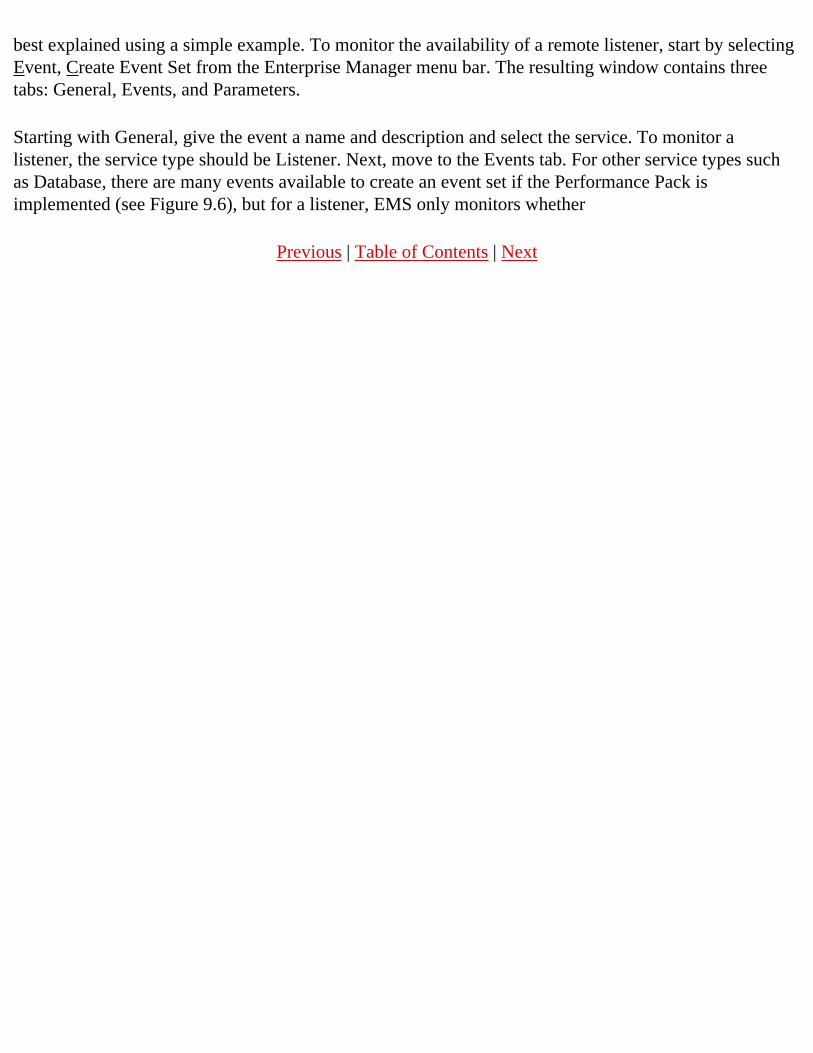
best explained using a simple example. To monitor the availability of a remote listener, start by selecting Event, Create Event Set from the Enterprise Manager menu bar. The resulting window contains three tabs: General, Events, and Parameters.
Starting with General, give the event a name and description and select the service. To monitor a listener, the service type should be Listener. Next, move to the Events tab. For other service types such as Database, there are many events available to create an event set if the Performance Pack is implemented (see Figure 9.6), but for a listener, EMS only monitors whether
Previous | Table of Contents | Next

Previous | Table of Contents | Next
Page 173
CHAPTER 10
PL/SQL Fundamentals
In this chapter
● Understanding PL/SQL 174 ● Understanding the PL/SQL Engine 175 ● Adding PL/SQL to Your Toolbox 179 ● Getting Started with PL/SQL 181 ● Language Tutorial 185
Page 174
Understanding PL/SQL
PL/SQL is a Procedural Language extension to Oracle's version of ANSI standard SQL. SQL is a non-procedural language; the programmer only describes what work to perform. How to perform the work is left to the Oracle Server's SQL optimizer. In contrast, PL/SQL, like any third-generation (3GL) procedural language, requires step-by-step instructions defining what to do next.
Like other industry-standard languages, PL/SQL provides language elements for variable declaration, value assignment, conditional test and branch, and iteration. Like C or Pascal, it is heavily block-oriented. It follows strict scoping rules, provides parameterized subroutine construction, and like Ada, has a container-like feature called a package to hide or reveal data and functionality at the programmer's discretion. It is a strongly typed language; data type mismatch errors are caught at compile and runtime. Implicit and explicit data type conversions can also be performed. Complex user-defined data structures are supported. Subroutines can be overloaded to create a flexible application programming environment.
Additionally, because it is a procedural wrapper for SQL, the language is well integrated with SQL. Certain language features enable it to interact with the Oracle RDBMS, performing set and individual row operations. The more you know about writing SQL, the better designed your PL/SQL programs will be.
PL/SQL provides a feature called Exception Handling to synchronously handle errors and similar events that may occur during processing. You'll learn how to embed exception handlers in your PL/SQL code

to deal with error conditions gracefully.
PL/SQL is not an objected-oriented language. It does have some features found in languages such as Pascal and Ada. If you're familiar with the syntax of Pascal, you will have no trouble learning PL/SQL. Unlike languages such as C and Pascal, pointers are not supported. PL/SQL is primarily a back-end development tool, where it interacts strictly with database tables and other database objects. Interaction with the operating system and external software components is handled through the supplied database packages.
PL/SQL is highly portable; it is standardized across all Oracle platforms. Because its data types are based on the database server's, the language is completely machine independent. You do not need to learn various flavors for UNIX, Windows NT, NetWare, and so on. A PL/SQL program will compile and run on any Oracle Server with no modifications required.
CAUTION
The Oracle Server imposes limitations on the size of a PL/SQL module, depending on the operating system. On NetWare 3.x it is limited to 32KB. For most flavors of UNIX and Windows NT, the module size is restricted to 64KB. Violating this limit can crash your database server or the server machine itself.
This portability also extends to 3GL programming languages. PL/SQL provides a standardized interface to various languages such as C and COBOL, via the Oracle-supplied precompilers. The precompilers support the ANSI standard for embedded SQL.
Page 175
Understanding the PL/SQL Engine
Before you look at PL/SQL as a language, you need to understand it in the executing environment.
Fitting into the Client/Server Environment
In a client/server configuration, the real bottleneck is typically the network. Connect a couple hundred users to the Oracle server via your compiled C, C++, Delphi, or COBOL program, and you'll have a very sluggish network system. The solution is to combine complex program segments, especially those performing reiterative or related SQL statements, into PL/SQL blocks. These blocks can be embedded in an OCI (Oracle Call Interface) program, or executed even more efficiently by moving them into the database itself as stored functions, procedures, and packages. Figure 10.1 shows the typical interaction between client applications with the Oracle server.

FIG. 10.1A typical client/serverenvironment.
PL/SQL is executed by the PL/SQL engine. This engine is part of the database server. Figure 10.2 illustrates internally how a PL/SQL block is handled.
Whatever tool you use, such as Oracle SQL*Plus, the tool must submit the PL/SQL source text to the Oracle Server. The PL/SQL engine scans, parses, and compiles the code. The compiled code is then ready to be executed. During execution, any SQL statements are passed to the SQL Statement Executor component for execution. The SQL Statement Executor performs the SQL or DML statement. The data set retrieved by the query is then available to the PL/SQL engine for further processing.
One advantage of using a PL/SQL block to perform a set of SQL statements, versus sending them individually, is the reduction in network traffic. Figure 10.3 illustrates this idea.
This alone can substantially improve an application's performance. Additionally, the SQL/DML statements can be treated as a single transaction. If the entire transaction succeeds, then all the
Page 176
modifications to the database can be committed. If any part fails, the entire transaction can be rolled back. Because complex logic can be included in the PL/SQL block, and thereby executed on the server, client program size and complexity is reduced.
FIG. 10.2The PL/SQL engine is acomponent of theOracle database server.
FIG. 10.3

Grouping several SQLstatements into one PL/SQL block reduces networktraffic.
Executing Stored SubprogramsA further refinement involves storing compiled, named PL/SQL blocks in the database. PL/SQL blocks will be referred to collectively in this chapter as stored subprograms or just subprograms. "Named" simply means the name of the subprogram that is included with its code, just like any C function or Pascal subroutine. Figure 10.4 illustrates how the PL/SQL engine calls stored subprograms.
Page 177
FIG. 10.4The PL/SQL engineruns stored subpro-grams.
These subprograms can perform complex logic and error handling. A simple anonymous or unnamed block (a block of PL/SQL code that isn't labeled with a name), embedded in a client application, can invoke these subprograms. This capability is generally referred to as a Remote Procedure Call (RPC). Subprograms can also call other subprograms. Because these subprograms are already compiled, and hopefully well tuned by the developer, they offer a significant performance improvement, as well as reduce application development by providing reusable building blocks for other applications or modules.
Shared SQL Areas Within the System Global AreaThe System Global Area (SGA) is a large chunk of memory allocated by the operating system to the Oracle Server. Within this memory, the Server maintains local copies of table data, cursors, user's local variables, and other sundry items.
When you compile any PL/SQL program, whether a named or unnamed block of code, the source and object code are cached in a shared SQL area. The space allocated to each PL/SQL block is called a cursor. The server keeps the cached program in the shared SQL area until it gets aged out, using a Least Recently Used algorithm. Any SQL statements inside the PL/SQL block are also given their own shared

SQL area.
When a named subprogram is compiled, its source code is also stored in the data dictionary.
The code contained in a subprogram is reentrant; that is, it is shareable among connected users. When an unnamed PL/SQL block is submitted to the server for execution, the server determines whether it has the block in cache by comparing the source text. If the text is exactly identical, character for character, including case, the cached, compiled code is executed. The same is true for SQL statements; if the query text is identical, the cached, parsed code can simply be executed. Otherwise, the new statement must be parsed first. By sharing executable code, a server-based application can achieve substantial memory savings, especially when hundreds of clients are connected.
Private SQL AreasIf several users are executing the same block of code, how does the server keep their data separated? Each user's session gets a private SQL area. This hunk of
Previous | Table of Contents | Next

Previous | Table of Contents | Next
Page 171
system is defined based on the type of workload (OLTP, DSS, or Batch), downtime tolerance, peak logical write rates, and application information. After the scope is defined, choose the Collect tab to define what data and how much data to collect for analysis. When the collection parameters are defined at the minimum level necessary to meet the tuning session scope, click the Collect button to acquire the required data. Before applying this process to a production database, practice in a test environment until the impact of the various options is understood and the amount of time consumed performing the specified activities is quantified.
Next, select the View/Edit tab to provide more detailed specification for the tuning session. This is where the specific tuning rules and thresholds are defined. Experienced tuners may want to alter some of the hundreds of rules based on the profile of the target database and personal knowledge and experience. For inexperienced tuners, it is an opportunity to see what Expert believes is good and bad.
From the Analyze tab, click the Perform Analysis button to begin the analysis process. After analysis is complete, select the Review Recommendations tab to get advice from Expert (see Figure 9.14). If recommendations are deemed reasonable, use the Implement tab to generate implementation scripts and new parameter files. Run the scripts and implement the new parameters to put Expert advice to work. If the advice does not seem correct, this can often be traced back to a rule that might require modification for the target database environment. Recollecting data is not required to develop new recommendations based on rule changes. Simply alter the rules to better reflect the environment of the target database and rerun the analysis.
FIG. 9.14These recommenda-tions are from anOracle sample file thatcomes with Expert.
Page 172
Expert provides the opportunity to aggregate the collected wisdom at Oracle Corporation and add the experience and knowledge of the local database administration team to a structured methodology for

performance management. Although most installations do not use this component of Enterprise Manager, it is probably most useful where it is least used—in small organizations with limited database tuning experience. Progressive database administrators in such environments should find a friend in Expert after even a short period of time using the tool.
Using the Enterprise Value-Added Products
Oracle provides several other value-added products that integrate with Enterprise Manager. Each meets specialized requirements for areas such as Web server management and processing of biometrics information such as fingerprints.
Replication Manager is useful for environments that make heavy use of Oracle8 replication features. Oracle Rdb for Windows NT provides tools to manage the Rdb database that Oracle acquired from Digital Equipment Corporation (DEC) several years ago. Oracle Fail Safe manages high availability environments implemented on Windows NT clusters. Oracle Biometrics works with specialized hardware to administer fingerprint identification used with the Advanced Networking Option (ANO). Oracle also integrates Web Server Manager and Security Server Manager with Enterprise Manager as value-added applications.
Using the Oracle Enterprise Manager Software Developer's Kit (SDK), developers build their own application integrated with Enterprise Manager to meet the specific needs of their environment. Several third-party applications are integrated with the Oracle Enterprise Manager. The functionality of these applications ranges from systems management functions such as transaction processing management connected through Oracle XA to specialized vertical market applications including a computerized medical record system. More third-party applications are under development.l
Previous | Table of Contents | Next

Previous | Table of Contents | Next
Page 168
Job configured, the Trace and Expert repositories on the client, remote intelligent agents on the node where Trace-enabled programs reside, Trace Collection Services on remote nodes (usually linked with the remote application), and Trace Formatter tables on remote nodes. Each application might require configuration as well. For example, at a minimum, Oracle8 must have the ORACLE_TRACE_ENABLE parameter set to TRUE before it will produce trace data. The setup is not trivial and should not be taken lightly. However, Trace is the key to providing the data necessary to take full advantage of the Enterprise Manager Performance Pack.
Managing Tablespaces
Tablespace Manager provides detailed information on storage utilization in tablespaces, data files, and rollback segments. A color-coded map of each piece of storage enables the database administrator to visualize the storage used by every database object, how many extents are used, and where the extents are placed in both the tablespace and data files (see Figure 9.12). This information is invaluable when tracking down I/O contention or tracking the progress of large database loads and index builds.
FIG. 9.12Selecting an extent inthe graphical displayhighlights other extentsin the same object.
In addition to the graphical display, there are two other tabs in the right application pane. The Space Usage tab displays the space utilization statistics, such as the row count and the average row length. The Extent Information tab shows information such as the extent count for the selected object and the data file where the selected extent resides.
Page 169
CAUTION

Most of the information under the Space Usage tab is produced by the ANALYZE SQL command. For objects with no statistics, generate statistics using ANALYZE or the Tablespace Analyzer Wizard. If the database is tuned for rules-based optimization and the CHOOSE optimization mode is employed, generating statistics may have an adverse performance impact. Likewise, if cost-based optimization is implemented and statistics are not available, performance might severely suffer.
Using Job, Tablespace Manager employs four wizards to change and analyze storage configurations. All four wizards submit jobs to the Enterprise Manager Job Scheduling component to perform the requested tasks. The Tablespace Analyzer Wizard analyzes selected tables, partitions, clusters, and indexes using the ANALYZE SQL command. The Tablespace Organizer Wizard defragments tables, partitions, and clusters using export and import utilities and rebuilds the indexes. It can also detect space that has not been used at the end of segments. The Defragmentation Wizard duplicates Tablespace Organizer defragmentation capabilities, but it is easier and quicker to use because it uses default options. The Coalesce Wizard combines adjacent free space into a single block. This is a particularly important technique for active operational databases where object sizes change frequently and temporary objects are routinely created and dropped. Unless a selected object contains adjacent free blocks, this wizard is disabled.
Monitoring Sessions
TopSessions enables database administrators to monitor database sessions and kill them if necessary due to inactivity or over-utilization of resources. This tool monitors all sessions or only the most active based on consumption of specified resources such as memory or I/O. Filtering provides a means to narrow the focus on sessions of interest when analyzing activity.
TIP
Before running TopSessions for Oracle8, run <ORACLE_HOME>/SYSMAN/SMPTSI80.SQL to ensure that tables required to perform all the functions are in place with appropriate permissions. Be aware that this script may not run "as is" and requires some editing to alter the ORACLE_HOME drive and name. It is still necessary to log in as SYS to explain access plans.
TopSessions can drill down into sessions to display exhaustive session statistics on redo, enqueue, cacheing, the operating system, parallel server, SQL, and other miscellaneous information. Examining active or open cursors (see Figure 9.13) reveals the SQL executed by each cursor and the access plan the SQL is using for execution. Locking information, including identification of blocking locks held by the session, is also available.

TIP
TopSessions can identify locks for a particular session, but for in-depth analysis of the entire locking picture, the tool to use is Lock Manager. Lock Manager displays either all locks held on the database or only blocking or waiting locks. Offending sessions can be killed directly from Lock Manager.
Page 170
FIG. 9.13By drilling down intoa session's open cursors,detailed access plans,are available.
Using Oracle Expert
Like Oracle Trace, Oracle Expert is an elaborate product with its own user's guide, consisting of 160 pages in the current release. Expert is more than just a product; it is the implementation of a performance management methodology. While other Performance Pack components provide information for database administrators to analyze, Expert applies a set of rules to the data to develop conclusions and make recommendations to improve performance. Expert considers trends that develop over time as well as current system conditions. As new database releases become available, the rules are updated to make recommendations on how to take advantage of new advanced features. As a result, Expert doubles as a mentor to help database administrators learn more about performance management and Oracle8.
Unfortunately, performance tuning is often neglected in favor of day-to-day requirements until serious performance problems affect the production database environment. Expert provides a means to automatically sift through performance data that might consume a large percentage of even a skilled database administrator's time. Expert doesn't replace the database administrator as a performance tuner. It does free the database administrator from the mundane task of screening mountains of data to find potential problems. With Expert, the performance tuning focus becomes how to deal with what Expert finds and enhancing Expert with more rules based on the experience and knowledge of the database administrator. Performance tuning becomes more efficient, effective, and rewarding.
To start an Expert Tuning session, from the menu, select File, New and start telling Expert about the areas it should analyze. The scope of the tuning session is defined based on requirements for instance

tuning, application tuning, and storage structure tuning. The profile of the
Previous | Table of Contents | Next

Previous | Table of Contents | Next
Page 178
memory contains a private copy of the variable data included in the subprogram. A private SQL area is also allocated for any SQL statements within the PL/SQL block. Figure 10.5 represents the scheme.
FIG. 10.5Shared and private SQLareas within the SGA.
The first time a stored subprogram is referenced, it must be loaded from the database into the SGA. Once loaded, it is available to every user. As long as it continues to be referenced by any user (not necessarily the one who first called it), the subprogram will remain in memory. Packages work the same way, except that a whole set of subprograms may be included in the package. The initial load may take longer, but now all these subprograms are available; there is no further disk hit. When a set of subprograms are expected to be invoked, you're better off having them all load at once. Packages offer this mechanism.
Fitting into the Client Environment
The PL/SQL engine may also be embedded in certain Oracle tools, such as SQL*Forms 4.5 and other Developer/2000 development tools. The main advantage here is programming in a familiar language. The client program can perform the computations contained in the local PL/SQL block, and send the SQL to the server or invoke stored PL/SQL portions. Again, this supports code reuse and simplifies the client program by handling portions of complex logic directly on the database server.
Server-Side Versus Client-Side Development
The developer must consciously decide how much complexity to hide on the server versus how much to keep in the client program. After years of developing client/server applications, the author suggests some guiding principles to follow:
● Reduce network traffic. Push some functionality on to the server. The network is typically the bottleneck in any client/server application.

Page 179
● Develop standard code. Standard code can be reused on new applications or when adding on to existing applications. This leverages past development effort.
● Strive for low coupling and high cohesiveness. Coupling occurs when one module is dependent on the specific contents of another module, such as when you use global variables instead of passing in parameters. Cohesiveness means putting like elements in the same place, such as bundling all math functions into one math library.
● Hide implementation details. This reduces client program complexity and decouples functionality from implementation. Decoupling is removing or avoiding module dependencies. When implementing top-down design, for example, defer the actual "how-to" by pushing implementation details down to the lower levels.
● Write modules in a generic manner. The more specific a module is, the less reusable it is. Look for patterns and common traits. This does not mean cram several different activities into a single module.
● Handle business rules in a consistent, centralized manner. This makes them more visible and reusable on future projects. If your business rules are ever-changing and spread out over many client program modules, you will have to locate and revise them all over the place—a process that is neither efficient nor maintainable.
NOTE
Clamage's Rule of Maintainability: A highly maintainable program module is one that requires little or no changes when the requirements for that module changes. An unmaintainable program is one that requires substantial modifications in order to incorporate new requirements. The above principles will help guide you toward the goal of building highly maintainable software.
Use stored subprograms to implement these principles. By providing standard libraries of stored subprograms, multiple and future client applications can take advantage of earlier, completed development. For example, business rules can be implemented as stored subprograms. If a rule changes, for example, how to compute a sales commission, just modify and recompile the appropriate stored program. Any dependent client programs need not change or even be recompiled, provided the stored subprogram's interface remains unchanged.
Packages are a good way to increase a subprogram's generality by allowing the subprogram name to be overloaded. Overloading simply means giving the same subprogram name to a set of code, usually with different data types or different numbers of arguments in the parameter list. For example, the addition operator is overloaded in nearly all computer languages to handle both integer and floating point arithmetic.
Adding PL/SQL to Your Toolbox

Stop for a minute and think about how you can use PL/SQL in your everyday tasks. You may not be involved in application development. As a DBA, you have to perform steady maintenance on the database. You can use PL/SQL to make your life easier.
Page 180
Energize Your SQL Scripts
Some SQL*Plus scripts can actually generate another script, such as listing the number of rows for every table in a tablespace. However, the scripts could be rewritten in PL/SQL, compiled, and stored in the database; thereby running much faster, without writing the intermediate script to a file.
Writing these kinds of scripts is also somewhat difficult; a PL/SQL script is more straightforward and easier to document and maintain. Additionally, a compiled PL/SQL program is readily shared among DBAs (especially if you're in a "24 x 7" shop). Instead of searching the hard drive for scripts, everyone will always know where they are and how to run them.
Stored subprograms can take parameters, which makes them extremely flexible. You can even write SQL*Plus front ends for them, collect user input and pass these values in, without having to know the order and types of the parameters.
Simplifying Database Administration
You probably have a good set of SQL scripts that give you information about your database in action. But after you understand PL/SQL, you'll envision a whole new set of programs that give you additional information on database performance, storage, user load, locks, and so on. PL/SQL eliminates the restrictions and limitations of plain SQL scripts.
You can automate many tasks, running them at set intervals by using the supplied packages. You can send system or application data to external performance monitors—written, perhaps, in C++ or Delphi—and use their powerful reporting and graphing features to display this information in real-time.
Some tools, such as Visual Basic, are easy to use. With the additional capabilities of PL/SQL, you can develop visual tools to simplify tasks such as running EXPLAIN PLAN and graphically viewing indexes and constraints on tables. Several upscale third-party tools were developed this way.
Getting Better Information with Less Hassle
You can write PL/SQL programs that use the data dictionary, for example, to show detailed index information for any particular table, even if it's in another schema. This is great if you're not logged on

as SYS or SYSTEM and you need some data dictionary information, and you don't want to have to reconnect. This is especially helpful to developers, who always need to access that kind of information. You can reverse-engineer any database object using PL/SQL, rebuilding a syntactically correct statement to re-create the object. This will save you the trouble of manually updating your scripts every time you alter a table or grant a new privilege.
If composing a large, complex SQL statement is difficult, you can break it up into smaller parts and run them together in a PL/SQL script. This is preferable to trying to join more than seven tables, after which the SQL Executor seems to bog down. Multi-table joins can be improved dramatically by doing the Master table lookups separately. Plus, it's easier to validate the output of a script when you know the reusable code in it is already working correctly.
Previous | Table of Contents | Next

Previous | Table of Contents | Next
Page 181
Designing Better Database Applications
You can use PL/SQL in stored procedures and packages to build better applications. A concerted effort to design and build reusable PL/SQL modules will reap long term benefits. With some thoughtful design and planning, you can:
● Leverage the effort in one application when building the next one. ● Spread the cost of building several related applications across all of them. ● Provide consistent interfaces to underlying tables and other objects. ● Simplify and optimize data access. ● Reduce application maintenance and deployment costs. ● Enforce coding standards.
Using PL/SQL is easy and fun. It has a relatively short learning curve as languages go. Experiment to determine what works well or at all. If you follow the steps detailed in this section, you should become productive in just a few days and, after only a few months, master PL/SQL sufficiently enough to achieve some sophisticated results.
Getting Started with PL/SQL
This section details some things the DBA must do before you can do much with PL/SQL. The architecture of the application environment in which you'll be working will also be explored.
Before you can really get into writing PL/SQL programs, you or your DBA must first do the following:
● Grant you (that is, your Oracle account name) the CREATE PROCEDURE privilege so you can create subprograms in your own schema. For new applications, you might want to create a special user name and schema (a particular tablespace).
● Grant you directly (not via a Role) SELECT, INSERT, UPDATE, or DELETE privileges on any database objects (for example, tables and sequences) in whatever schema for which you may be writing PL/SQL programs. A stored subprogram or package can only reference objects that the owner of the subprogram (you) has access rights to directly (not via a role).
● Make sure the appropriate Oracle-supplied packages have been compiled, and you have EXECUTE privilege on them. You will find them in the directory <ORACLE_HOME>/rdbms<version>/admin/ where <ORACLE_HOME> is the Oracle home directory (shown either in the UNIX shell variable of the same name or in the Windows Registry) and <version> is the database version. The names of the package scripts have the general form of dbms*.sql. For

example, on the author's Win95 machine, dbmssql.sql is in d:\orawin95\rdbms72\admin. ● Make sure there is sufficient storage available for your stored subprograms and packages. These
objects make additional data dictionary entries in the SYSTEM tablespace. The DBA may create a default tablespace for your own local copies of tables and indexes, so you aren't mucking with Production objects.
Page 182
● Make sure the shared and private SQL areas in the System Global Area (SGA) are sufficiently large to handle the anticipated load from running PL/SQL scripts and subprograms.
● Make sure you have access to the SQL*Plus application or a suitable third-party tool.
Once these things are in place, you're ready to start developing PL/SQL programs!
Understanding the Schema of Things
In abstract terms, a schema is a logical collection of related database objects, such as tables, indexes, and views. A schema is a developer's-eye view of the database objects of interest, such as are shown on an Entity-Relationship Diagram (or ERD).
In an Oracle database, a schema is a logical collection of objects stored within one or more tablespaces. Because it is a logical collection, several applications can share schemas, or cross schema boundaries into other schemas. The relational organization of schema objects is strictly as the DBA and developers see it, which is why a "roadmap," such as an ER diagram, is critical to the success of any database-related software development. A tablespace, in turn, is a logical storage area that maps to one or more physical files out on disk. Figure 10.6 illustrates this organization.
FIG. 10.6Applications, schemas,tablespaces, anddatabase files areorganized hierarchically.
Typically, a schema has exactly one owner (that is, an Oracle user account) responsible for creating, altering, and dropping these objects. This owner then grants access privileges to other users, either directly or via roles. If you're not the owner of these objects, you qualify references to the objects by specifying which tablespace they are in using dot notation, as with SELECT CUST_NAME FROM MKG.LEADS.

Managing Your PL/SQL Code After they have been thoroughly tested and validated in your own development schema, your stored PL/SQL programs are likely to become objects managed by the schema owner. In a complex development environment with many developers, it becomes critical to determine who is the owner of
Page 183
the source code and where it is kept. When a module is being worked on, it is in a state of flux. The developer can make significant changes to a private copy, some of which may be backed out later. It's strongly recommended that you use a Code Management System (CMS) to control the one official version of the source code. When the module has been thoroughly tested and accepted for Production, the new version is placed in the CMS, and the schema owner can compile the new version. The quickest way to shoot yourself in the foot is to lose track of which copy is the one known good version. In the long run, just keeping different subdirectories for different versions is a poor code management strategy.
There is no correspondence between schemas and tablespaces; one or more schemas may be stored in a single tablespace, or one schema may be broken up into separate tablespaces. In practice, it is generally a good idea to store a schema in its own set of tablespaces, along with a good set of documentation. For example, tables may be stored in one tablespace and indexes in another. Conceptually, both tablespaces are included in the same schema.
TIP
PL/SQL developers should have their own default tablespaces to play around in, preferably on a non-Production database. You can create your own private tables and indexes with which to experiment. This way, if you inadvertently corrupt a temporary, local copy of a Production table, who cares? Whereas the alternative could result in an abrupt end in your career (at least as far as your current workplace goes). Additionally, any stored programs or packages you compile are strictly local to within your schema (stored in the data dictionary alongside subprograms belonging to other schemas), so you can make experimental changes to Production code in a safe development environment.
CAUTION
The caveat to this scheme is to take care with object references. If it's in your default tablespace, you don't need to qualify the reference with the tablespace name; otherwise, you must qualify it in order for it to be properly found. If an object by the same name is in more than one tablespace, qualify the reference. You can use synonyms for unqualified objects in PL/SQL code to provide the qualifier.

As a pragmatic consideration, some applications may easily cross schema boundaries, whereas core applications might focus on one schema. For example, a marketing application may have been developed to automate this one department. Later, upper management may request a high-level view of the entire enterprise, requiring a new application to obtain data from several schemas. The work you do in one application may be reused in another, so always keep an eye toward making PL/SQL modules generic enough to be used in multiple contexts.
Your Basic PL/SQL Development Environment
PL/SQL code is developed using your favorite text editor and the Oracle-supplied SQL*Plus application, or one of the several fine third-party development toolkits. If you're in a UNIX environment, it's a good idea to have a couple of sessions up—one running a text editor such as vi or emacs, and another session running SQL*Plus. If you're running Windows, you can use Notepad (or a real programmer's editor) and have a SQL*Plus session up.
Previous | Table of Contents | Next

Previous | Table of Contents | Next
Page 239
CHAPTER 11
Using Stored Subprograms and Packages
In this chapter
● Defining Stored Subprograms and Packages 240 ● Building and Using Stored Programs 240 ● Debugging with Show Errors 248 ● Checking the State of a Stored Program or Package 255 ● Building and Using Packages 256 ● Creating a Real-World Example 263
Page 240
Defining Stored Subprograms and Packages
The real application development begins when you start building stored subprograms and packages, which are persistent code modules that are compiled and stored in the database. They are shareable, reentrant, and reusable software that you design. They are callable from other PL/SQL modules, SQL statements, and client-side applications in languages that support remote procedure calls.
Whenever you compile a stored subprogram or package, the source code, compiled code, compilation statistics, and any compilation errors are stored in the data dictionary. Various data dictionary views help you visualize these entities. You can get information about modules you compile with the USER_ views; you can get some restricted information about modules other folks compiled and granted you access to with the ALL_ views; and you can get all information anyone compiled with the DBA_ views, provided you have DBA rights. These views are listed in Table 11.1 (for simplicity, listed as DBA_ views).
Table 11.1 Data Dictionary Views for Stored Subprograms and Packages
View Description

DBA_SOURCE Textual source code for all compiled modules.
DBA_ERRORS Textual listing of any compilation errors for all modules.
DBA_OBJECT_SIZE Statistics for compiled modules, such as validity, source, and object sizes.
DBA_OBJECTS Catalog of compiled modules (stored procedures, functions, packages, package bodies).
DBA_DEPENDENCIES List of object dependencies, such as tables referenced in packages.
No views exist to expose the object code because you don't need to see it. All you need to know is that it's in there and whether it's valid. A compiled module becomes invalid when a dependent object is changed or removed, such as when a column is added or a table dropped. If a stored module becomes invalid, it first must be recompiled, either automatically by the server or manually by the owner.
Building and Using Stored Programs
The syntax for creating stored subprograms is very similar to that for defining subprograms in anonymous PL/SQL blocks. Stored subprograms have all the same features of the sub-programs you learned to write in the previous chapter, plus some additional ones. Let's make a stored function out of that bool_to_char function you saw earlier (see Listing 11.1).
Page 241
Listing 11.1 bool2chr.sql—Stored Subprograms Make for Reusable Code
CREATE OR REPLACE FUNCTION bool_to_char(Pbool IN BOOLEAN)RETURN VARCHAR2 IS str VARCHAR2(5); -- capture string to returnBEGIN IF (Pbool) THEN -- test Boolean value for TRUE str := `TRUE'; ELSIF (NOT Pbool) THEN -- FALSE str := `FALSE'; ELSE -- must be NULL str := `NULL'; END IF; -- test Boolean value RETURN (str);

END bool_to_char;/
The server replies:
Function created.
That's all you get. The server doesn't execute the program; it compiles the program so that you can execute it later when called from other PL/SQL blocks.
NOTE
The CREATE OR REPLACE syntax creates a new function or replaces an existing one. This means you don't make incremental recompilations or source changes to stored code; you totally replace them with new versions.
CAUTION
Good source code management is required when using CREATE OR REPLACE. Once you replace a subprogram, the old source is gone forever from the data dictionary. It also means you can only have one object of this name in your schema.
Now let's run this newly created stored function using an unnamed PL/SQL block, as shown in Listing 11.2.
Listing 11.2 testbool.sql—Executing a Stored Subprogram
SET SERVEROUTPUT ONBEGIN DBMS_OUTPUT.enable; DBMS_OUTPUT.put_line(bool_to_char(TRUE)); DBMS_OUTPUT.put_line(bool_to_char(FALSE)); DBMS_OUTPUT.put_line(bool_to_char(NULL));END;/
Page 242
This example pretty much exhausts the possibilities for all possible values returned by the stored function. It is called a Unit Test. For each input, verify the output. The input values should test all
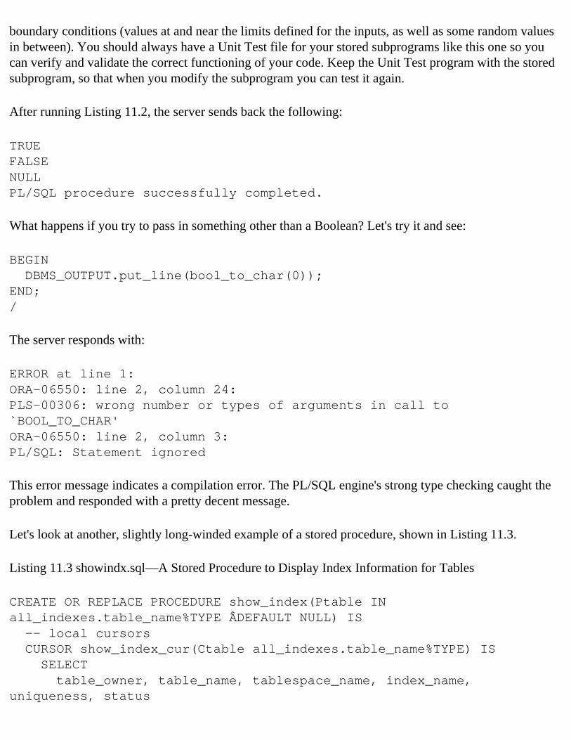
boundary conditions (values at and near the limits defined for the inputs, as well as some random values in between). You should always have a Unit Test file for your stored subprograms like this one so you can verify and validate the correct functioning of your code. Keep the Unit Test program with the stored subprogram, so that when you modify the subprogram you can test it again.
After running Listing 11.2, the server sends back the following:
TRUEFALSENULLPL/SQL procedure successfully completed.
What happens if you try to pass in something other than a Boolean? Let's try it and see:
BEGIN DBMS_OUTPUT.put_line(bool_to_char(0));END;/
The server responds with:
ERROR at line 1:ORA-06550: line 2, column 24:PLS-00306: wrong number or types of arguments in call to `BOOL_TO_CHAR'ORA-06550: line 2, column 3:PL/SQL: Statement ignored
This error message indicates a compilation error. The PL/SQL engine's strong type checking caught the problem and responded with a pretty decent message.
Let's look at another, slightly long-winded example of a stored procedure, shown in Listing 11.3.
Listing 11.3 showindx.sql—A Stored Procedure to Display Index Information for Tables
CREATE OR REPLACE PROCEDURE show_index(Ptable INall_indexes.table_name%TYPE ÂDEFAULT NULL) IS -- local cursors CURSOR show_index_cur(Ctable all_indexes.table_name%TYPE) IS SELECT table_owner, table_name, tablespace_name, index_name, uniqueness, status

FROM all_indexes WHERE (Ctable IS NULL OR table_name = Ctable) -- one table or all ORDER BY table_owner, table_name, index_name; -- local constants TB CONSTANT VARCHAR2(1) := CHR(9); -- tab character
Previous | Table of Contents | Next

Previous | Table of Contents | Next
Page 237
binary_search(numarr, 100, isfound, rowout); DBMS_OUTPUT.put_line(`FOUND=' || bool_to_char(isfound) || `, ROW=' || TO_CHAR(rowout) || ` SB=1'); binary_search(numarr, 145, isfound, rowout); DBMS_OUTPUT.put_line(`FOUND=' || bool_to_char(isfound) || `, ROW=' || TO_CHAR(rowout) || ` SB=11'); binary_search(numarr, 108, isfound, rowout); DBMS_OUTPUT.put_line(`FOUND=' || bool_to_char(isfound) || `, ROW=' || TO_CHAR(rowout) || ` SB=4'); binary_search(numarr, 105, isfound, rowout); DBMS_OUTPUT.put_line(`FOUND=' || bool_to_char(isfound) || `, ROW=' || TO_CHAR(rowout) || ` SB=4');END; -- bintest/
The output from the server is
FOUND=FALSE, ROW=1 SB=1FOUND=FALSE, ROW=13 SB=13FOUND=TRUE, ROW=1 SB=1FOUND=TRUE, ROW=11 SB=11FOUND=TRUE, ROW=4 SB=4FOUND=FALSE, ROW=4 SB=4PL/SQL procedure successfully completed.
Note the OUT parameter mode, which means output only. This means inside the procedure, this variable can only be written to. If you need to read and write from a parameter variable, declare it as IN OUT.
Does that binary to char conversion routine look familiar? Wouldn't it be nice not to have to paste into every PL/SQL program that needs it?
Default Parameter ValuesParameters can receive default values, to be used when the parameter is not provided in the actual call to the subprogram. This makes the subprogram appear as if it can have a variable list of parameters.
DECLARE ... -- types, constants, variables

FUNCTION get_data (Pkey IN CHAR, Pflag IN BOOLEAN DEFAULT FALSE, Psort IN CHAR DEFAULT ` `) RETURN VARCHAR2 IS ... -- function implementationBEGIN -- executable code IF get_data(key1) THEN -- valid call (Pflag, Psort defaulted) ... ELSIF get_data(key2, TRUE) -- valid call (Psort defaulted) ... ELSIF get_data(key3, , `ASCENDING') THEN -- invalid!
Note the use of the keyword DEFAULT. You could also use the assignment operator (:=). As a coding convention, only DEFAULT is used in this context, to distinguish this semantically unusual construction from the more straightforward assignment upon declaration.
Page 238
Both default parameters can be left off intentionally, so in the first call to get_data the flag parameter is defaulted to FALSE, and the sort parameter is defaulted to spaces. This makes for a very clean coding style where you only specify the parameters of interest to you. Note, however, that you cannot skip a default parameter and provide the next one because this notation for specifying parameters is positional. The positions of the parameters is significant. You cannot try to use a placeholder, such as the extra comma above.
Positional and Named NotationYou can use an alternate notation, however, called named notation to specify parameters in any order. You provide the name of the parameter along with the value.
ELSIF get_data(key3, Psort => `ASCENDING') THEN -- valid (Pflag defaulted)
You can start off left to right using positional notation, then switch to named notation, which is known as mixed notation. Once you use named notation, you must then stick with it for subsequent parameters. Named notation can be used for any parameter, not just any that were defaulted.
ELSIF get_data(key3, Psort => `ASCENDING', Pflag => TRUE) THEN -- right ...ELSIF get_data(Pkey => key3, `ASCENDING', Pflag => TRUE) THEN -- wrong!
Although this seems convenient and unusual among programming languages, I've never needed it. But if

you had a bunch of parameters and nearly every parameter was defaulted and you wanted to have maximum flexibility calling the subroutine, this is practically indispensable.
Built-in FunctionsNearly all the built-in functions and operators you use in SQL can also be used in PL/SQL expressions and procedural statements. There are only a few exceptions to this rule.
You cannot use `= ANY (…)' in an expression. Instead, use the IN operator, as in:
IF (key IN (`A', `B', `C')) THEN -- acts like an OR conditional
You can still use operators such as BETWEEN, IS NULL, IS NOT NULL, LIKE, and so on.
You cannot use DECODE in procedural statements. Also, none of the SQL group functions are allowed in procedural statements. They don't make much sense in this context, either. Of course, there are no such restrictions for SQL statements embedded in PL/SQL.
You have seen how to use SQLCODE to trap the numeric exception error value. SQLERRM (sqlcode) is used to convert the SQLCODE value to the error message string associated with the exception. All the other built-in functions are fair game.
Previous | Table of Contents | Next

Previous | Table of Contents | Next
Page 233
evaluated. An OUT parameter may only appear on the left side of an assignment statement. An IN OUT parameter can appear anywhere.
In general, use the most restrictive mode as needed for the subprogram. This provides the greatest protection from programming errors where variables are inadvertently trashed during a subprogram execution.
Try coding all your single row lookup routines as procedures. Follow the same coding style for single-row lookups. Pass in the key values, a return row type record variable, and a status indicator. This style has the advantage of encapsulating the SQL statement or cursor in order to handle exceptions inline, as well as making for reusable code fragments. It is also an easily maintainable style. Listing 10.27 shows an example of this style:
Listing 10.27 table.sql—A Standardized Coding Style Lends Itself to Maintainable Code
DECLARE -- constants TB CONSTANT VARCHAR2(1) := CHR(9); -- TAB -- variables status NUMERIC; table_rec all_tables%TYPE; -- routines PROCEDURE get_table(Powner IN all_tables.owner%TYPE, Ptable IN all_tables.table_name%TYPE, Prec OUT all_tables%TYPE, Pstatus IN OUT NUMERIC) IS -- local cursors CURSOR table_cur(Cowner all_tables.owner%TYPE, Ctable all_tables.table_name%TYPE) IS SELECT * FROM all_tables WHERE owner = Cowner AND table_name = Ctable; -- local variables Lowner all_tables.owner%TYPE; Ltable all_tables.table_name%TYPE; BEGIN Pstatus := 0; -- OK

Lowner := UPPER(Powner); Ltable := UPPER(Ptable); OPEN table_cur(Lowner, Ltable); FETCH table_cur INTO Prec; IF (table_cur%NOTFOUND) THEN RAISE NO_DATA_FOUND; END IF; CLOSE table_cur; EXCEPTION WHEN OTHERS THEN BEGIN Pstatus := SQLCODE; -- capture error code IF (table_cur%ISOPEN) THEN -- close the open cursor
continues
Page 234
Listing 10.27 Continued
CLOSE table_cur; END IF; Prec := NULL; -- clear return values and display input values DBMS_OUTPUT.put_line(`get_table: ` || SQLERRM(Pstatus)); DBMS_OUTPUT.put_line(`OWNER = ` || `<` || Lowner || `>'); DBMS_OUTPUT.put_line(`TABLE = ` || `<` || Ltable || `>'); EXCEPTION WHEN OTHERS THEN NULL; -- don't care (avoid infinite loop) END; END get_table;BEGIN -- display storage parameters for a given table DBMS_OUTPUT.enable; DBMS_OUTPUT.put_line(`TABLE' || TB || `TABLESPACE' || TB || `INITIAL' || TB || `NEXT' || TB || `MAX'); DBMS_OUTPUT.put_line(RPAD(`-', 43, `-')); -- just an underline get_table(`scott', `dept', table_rec, status); IF (status = 0) THEN DBMS_OUTPUT.put_line( table_rec.table_name || TB || table_rec.tablespace_name || TB || table_rec.initial_extent || TB ||

table_rec.next_extent || TB || table_rec.max_extents); END IF; get_table(`scott', `garbage', table_rec, status); IF (status = 0) THEN DBMS_OUTPUT.put_line( table_rec.table_name || TB || table_rec.tablespace_name || TB || table_rec.initial_extent || TB || table_rec.next_extent || TB || table_rec.max_extents); END IF;END;/
The server returns the following:
TABLE TABLESPACE INITIAL NEXT MAX-------------------------------------------DEPT USER_DATA 10240 10240 121get_table: ORA-01403: no data foundOWNER = <SCOTT>TABLE = <GARBAGE>PL/SQL procedure successfully completed.
If you anticipate an exact match using a unique key, manage the cursor yourself and perform exactly one fetch. When detecting no rows, close the cursor in the exception handler, rather than inside the conditional block (it has to be closed in the exception block anyway, so why code it three times?). Note that you must raise the predefined exception NO_DATA_FOUND,
Page 235
because the fetch does not generate one automatically. The input values are converted to uppercase using local variables because the converted values are used in more than one place.
Also take note of the additional information displayed by the exception handler. Why not take the opportunity to show the key values that the exception occurred on? This would be especially valuable when processing a large number of rows. This information could also have been dumped to an error table for post mortem analysis.
You might be thinking, "I can get the same information with a simple SELECT statement. What does all this buy me?" In the larger scheme of things, canned queries are more efficient because they can be

found in the shared SQL area and reused. The manual control of the cursor with its single fetch is certainly more efficient, especially when it is run thousands of times over and over. Remember, your goal is to write efficient applications. After you have the row that was found, you can programmatically do anything you want with it. You have total flexibility and control, yet the underlying procedure is coded once and reused.
Listing 10.28 shows another example that implements a binary search on a PL/SQL table containing numeric values.
Listing 10.28 bintest.sql—A Binary Search Routine Made Easy to Use with a Procedure
SET SERVEROUTPUT ONDECLARE -- constants FIXED_TOP CONSTANT NUMBER := 12; -- fixed # of elements -- data types TYPE NUMARR_TYPE IS TABLE OF NUMBER INDEX BY BINARY_INTEGER; -- global variables numarr NUMARR_TYPE; isfound BOOLEAN; rowout NUMBER;
-- routines PROCEDURE binary_search( -- binary search on sorted array Parr IN NUMARR_TYPE, Pnum IN NUMBER, Pfound OUT BOOLEAN, Prow OUT NUMBER) IS local_found BOOLEAN := NULL; top BINARY_INTEGER := FIXED_TOP; bottom BINARY_INTEGER := 1; middle BINARY_INTEGER := NULL; BEGIN local_found := FALSE; LOOP -- binary search middle := ROUND((top + bottom) / 2); -- find middle IF (Parr(middle) = Pnum) THEN -- exact match local_found := TRUE; -- match succeeded EXIT; -- break
continues

Page 236
Listing 10.28 Continued
ELSIF (Parr(middle) < Pnum) THEN -- GO UP bottom := middle + 1; ELSE -- GO DOWN top := middle - 1; END IF; -- test for match IF (bottom > top) THEN -- search failed IF (Pnum > Parr(middle)) THEN middle := middle + 1; -- MAY BE OUTSIDE ARRAY! END IF; -- insert after EXIT; END IF; -- failed END LOOP; -- search Pfound := local_found; Prow := middle; EXCEPTION WHEN OTHERS THEN DBMS_OUTPUT.PUT_LINE(SQLERRM(SQLCODE)); DBMS_OUTPUT.PUT_LINE(TO_CHAR(middle)); END binary_search;
FUNCTION bool_to_char(Pbool IN BOOLEAN) -- convert Boolean to char RETURN VARCHAR2 IS str VARCHAR2(5); -- capture string to return BEGIN IF (Pbool) THEN -- test Boolean value for TRUE str := `TRUE'; ELSIF (NOT Pbool) THEN -- FALSE str := `FALSE'; ELSE -- must be NULL str := `NULL'; END IF; -- test Boolean value RETURN (str); END bool_to_char;BEGIN -- bintest executable code DBMS_OUTPUT.enable; numarr(1) := 100; -- fill array with numbers in order numarr(2) := 103; numarr(3) := 104; numarr(4) := 108;

numarr(5) := 110; numarr(6) := 120; numarr(7) := 121; numarr(8) := 122; numarr(9) := 130; numarr(10) := 140; numarr(11) := 145; numarr(12) := 149; binary_search(numarr, 90, isfound, rowout); DBMS_OUTPUT.put_line(`FOUND=' || bool_to_char(isfound) || `, ROW=' || TO_CHAR(rowout) || ` SB=1'); binary_search(numarr, 150, isfound, rowout); DBMS_OUTPUT.put_line(`FOUND=' || bool_to_char(isfound) || `, ROW=' || TO_CHAR(rowout) || ` SB=13');
Previous | Table of Contents | Next

Previous | Table of Contents | Next
Page 243
-- local record variables show_index_rec show_index_cur%ROWTYPE; -- based on cursor old_index_info show_index_cur%ROWTYPE; -- used to detect control break -- local variables status NUMERIC; local_table all_indexes.table_name%TYPE;BEGIN status := 0; local_table := UPPER(Ptable); -- make upper case old_index_info.table_owner := `GARBAGE_OWNER'; -- initialize old_index_info.table_name := `GARBAGE_TABLE'; IF (local_table IS NULL) THEN -- one table or all? DBMS_OUTPUT.put_line(`User ` || USER || `: Index Information forAll ÂTables'); ELSE
DBMS_OUTPUT.put_line(`User ` || USER || `: Index Information for Table `|| Âlocal_table); END IF; -- one table or all? OPEN show_index_cur(local_table); LOOP -- get index information FETCH show_index_cur INTO show_index_rec; EXIT WHEN show_index_cur%NOTFOUND; IF (old_index_info.table_owner != show_index_rec.table_owner OR old_index_info.table_name != show_index_rec.table_name) THEN-- Âcontrol break DBMS_OUTPUT.put_line(TB); -- double spacing between tables END IF; DBMS_OUTPUT.put_line(`Table Owner: ` || show_index_rec.table_owner || TB || `Table: ` || show_index_rec.table_name);
DBMS_OUTPUT.put_line(`Index: ` || show_index_rec.index_name
Â|| TB || ` in ` || show_index_rec.tablespace_name || TB ||

show_index_rec.uniqueness || TB|| show_index_rec.status); old_index_info := show_index_rec; -- copy new values to old END LOOP; -- get index information CLOSE show_index_cur;EXCEPTIONWHEN OTHERS THEN BEGIN status := SQLCODE; DBMS_OUTPUT.put_line(`show_index: ` || SQLERRM(status)); -- displayerror message IF (show_index_cur%ISOPEN) THEN -- close any open cursors CLOSE show_index_cur; END IF;
EXCEPTION WHEN OTHERS THEN NULL; -- don't care END;END show_index;/
This time, the server responds with:
Procedure created.
Page 244
To execute this procedure, you can call it from an anonymous PL/SQL block, or you can use the EXECUTE command for one-liners.
NOTE
The EXECUTE command can only be used to run one-line statements. If your statement spans two or more lines, you must use an anonymous PL/SQL block (using BEGIN .. END). If you can cram two or more statements onto a single line, you can still use EXECUTE. In fact, EXECUTE expands to a BEGIN .. END block on one line. It's just a shorthand.
EXECUTE show_index(`DEPT');

On my system I get:
User SYSTEM: Index Information for Table DEPT
Table Owner: SYSTEM Table: DEPTIndex: DEPT_PRIMARY_KEY in USER_DATA UNIQUE VALID
PL/SQL procedure successfully completed.
The first time I run this stored procedure, I have to wait for the server to load it into memory. On subsequent calls, running it is much faster because it's already loaded.
This particular example shows some fine features you'll want in your own stored procedures. I always try to be consistent with the organization of local variable declarations, always putting them in the same order. Also, notice the block inside the exception handler to close the cursor in case an error leaves it open. If you don't do this and you do have an exception, the next time you run the stored procedure you will immediately bomb with a CURSOR_ALREADY_OPEN exception. Your users would have to reconnect in order to clear the open cursor because the cursor remains open for the duration of a session until either the cursor is closed or the session is terminated.
If the user wants all tables and their indexes that are visible, simply drop the single input parameter (and parentheses in this case), as with:
EXECUTE get_index;
You have to put yourself in your users' (in this case, developers') shoes to anticipate the various ways in which they might want to use this tool. Better yet, go ask them. You'll be surprised at the answers you'll get.
Calling Stored Programs from SQL
Suppose you aren't satisfied with the Oracle-supplied TO_NUMBER() built-in function. Your complaint with it might be that when a character-to-number conversion fails because the string doesn't represent a valid number, the SQL fails and terminates abruptly. What you'd prefer is that, at the very least, the error is handled gracefully so that processing can continue with the rest of the data set. Let's try to cure this problem with a stored function, as shown in Listing 11.4.
Page 245
Listing 11.4 char2num.sql—Character-to-Number Conversion

CREATE OR REPLACE FUNCTION char_to_number(Pstr IN VARCHAR2, Pformat INVARCHAR2 DEFAULT NULL)RETURN NUMBER ISBEGIN IF Pformat IS NULL THEN -- optional format not supplied RETURN (TO_NUMBER(Pstr)); ELSE RETURN (TO_NUMBER(Pstr, Pformat)); -- format supplied END IF; -- test for optional formatEXCEPTIONWHEN OTHERS THEN -- unknown value RETURN (NULL);END char_to_number;/
You can run this stored function in two ways:
● From a PL/SQL block ● Within an SQL statement
First, try it from a PL/SQL block, as shown in Listing 11.5.
Listing 11.5 testc2n1.sql—Testing char_to_number() from a PL/SQL Block
DECLARE v VARCHAR2(1) := 0; w VARCHAR2(10) := `999.999'; -- try a floating point number x VARCHAR2(11) := `+4294967295'; -- try a big positive number y CHAR(11) := `-4294967296'; -- try a big negative number z VARCHAR2(10) := `garbage'; -- this is NOT a number!BEGIN -- stored function returns NULL on error, so convert NULL to error message DBMS_OUTPUT.put_line(v || ` is ` || NVL(TO_CHAR(char_to_number(v)), `NOTA ÂNUMBER!')); DBMS_OUTPUT.put_line(w || ` is ` || NVL(TO_CHAR(char_to_number(w)), `NOTA ÂNUMBER!')); DBMS_OUTPUT.put_line(x || ` is ` || NVL(TO_CHAR(char_to_number(x)), `NOTA ÂNUMBER!'));

DBMS_OUTPUT.put_line(y || ` is ` || NVL(TO_CHAR(char_to_number(y)), `NOTA ÂNUMBER!')); DBMS_OUTPUT.put_line(z || ` is ` || NVL(TO_CHAR(char_to_number(z)), `NOTA ÂNUMBER!'));END;/
The server responds:
0 is 0999.999 is 999.999+4294967295 is 4294967295-4294967296 is -4294967296garbage is NOT A NUMBER!
Page 246
PL/SQL procedure successfully completed.
Okay, now let's try it in a SQL statement, as shown in Listing 11.6.
Listing 11.6 testc2n2.sql—Running char_to_number() from SQL
SELECT `0' str, NVL(TO_CHAR(char_to_number(`0')), ` IS NOT A NUMBER!') num FROM DUAL;SELECT `999.999' str, NVL(TO_CHAR(char_to_number(`999.999')), ` IS NOT A NUMBER!') numFROM ÂDUAL;SELECT `+4294967295' str, NVL(TO_CHAR(char_to_number(`+4294967295')), ` IS NOT A NUMBER!') numFROM ÂDUAL;SELECT `-4294967296' str, NVL(TO_CHAR(char_to_number(`-4294967296')), ` IS NOT A NUMBER!') numFROM ÂDUAL;SELECT `garbage' str, NVL(TO_CHAR(char_to_number(`garbage')), ` IS NOT A NUMBER!')

numFROM ÂDUAL;
And you get the same answers as above. It looks kind of goofy converting back to a string when you just got through converting from a string to number, but still it verifies the operation of the stored function, particularly in the last query shown.
Just for fun, let's write the converse of bool_to_char(), called appropriately char_to_bool() (see Listing 11.7).
Listing 11.7 chr2bool.sql—Converting a String to Boolean
CREATE OR REPLACE FUNCTION char_to_bool(Pstr IN VARCHAR2) RETURN BOOLEAN IS Lstr VARCHAR2(32767); -- max string length Lbool BOOLEAN := NULL; -- local Boolean value (default)BEGIN Lstr := UPPER(LTRIM(RTRIM(Pstr))); -- remove leading/trailing spaces,
Âuppercase IF (Lstr = `TRUE') THEN Lbool := TRUE; ELSIF (Lstr = `FALSE') THEN Lbool := FALSE; END IF; RETURN(Lbool);END char_to_bool;/
Now, let's test it with the PL/SQL statement shown in Listing 11.8.
Listing 11.8 testc2b1.sql—Testing char_to_bool() in a PL/SQL Block
BEGIN IF (char_to_bool(` true `)) THEN DBMS_OUTPUT.put_line(`''Tis True!');
Previous | Table of Contents | Next

Previous | Table of Contents | Next
Page 247
END IF; IF (NOT char_to_bool(` False')) THEN DBMS_OUTPUT.put_line(`''Tis Untrue!'); END IF; IF (char_to_bool(`NULL `) IS NULL) THEN DBMS_OUTPUT.put_line(`Don''t Care!'); END IF;END;/
The server responds:
'Tis True!'Tis Untrue!Don't Care!PL/SQL procedure successfully completed.
Now try it in a SQL statement.
SELECT char_to_bool(`true') FROM DUAL;
But this time, the server responds:
ERROR:ORA-06550: line 1, column 12:PLS-00382: expression is of wrong typeORA-06550: line 1, column 7:PL/SQL: Statement ignored
no rows selected
What happened? There's no Boolean data type in SQL. The return value of the function is an unknown SQL data type. The PL/SQL engine has determined that the data type is inappropriate within the context of a SQL statement. The SQL engine subsequently returns no rows.
Calling Stored Programs from PL/SQL

You've already seen how to invoke a stored subprogram from a PL/SQL block. What's a high value use for them? Have you ever tried to compose a query that has a 14-table join? Instead, create a bunch of single-row lookup routines for each master table whose key you would have used in a join. Then, in a PL/SQL block, code just the minimal tables required to drive a cursor loop. Inside the loop, perform the single-row lookups for the attendant data values. Using this technique, I've seen speed improvements of 4,000%. Queries that used to run in 20 minutes can be run in 30 seconds or faster, using this technique. If you're using some sort of report writer to format the output, you can write the data to a temporary table, which can then be scanned by the reporting tool. Obviously, this slows things down somewhat, but it's still faster than bogging down the Oracle Server with a huge, complex query. Plus, it's easier to verify the correctness of the output. If you rigorously test the single-row lookup routines, the only facet you'll have to validate is the substantially smaller query.
Page 248
Now think about how many times you had to code an outer join in a complex query. In a PL/SQL block, it's a piece of cake to test the single-row lookup for no data found, and skip to the end of the loop or carry on, as needed. For example, a Claims Processing program might have a loop in it that looks something like this:
LOOP -- process all claims for the period selected FETCH claims_cur INTO claims_rec; EXIT WHEN claims_cur%NOTFOUND; -- get related table info get_claimant_info(claims_rec.claimant_ssn, status); get_provider_info(claims_rec.provider_id, status); get_approval_info(claims_rec.approvedby, status); IF (status != 0) THEN -- no approval on file! GOTO SKIPIT; -- skip processing claim END IF; ... -- more single row lookups, claims processing <<SKIPIT>> -- continue with next claimEND LOOP; -- process all claims for the period selected
where status is passed back the SQLCODE result value of the single-row lookup. To make this example really useful, you need to dump information about why the claim wasn't processed (no approval) to some sort of application error table. Even better, inside the lookup routine you could dump the lookup key and error code to an errors table of your design. Then you could later determine the subroutine and key values that caused a claim to go unprocessed. The calling program could then dump additional data ( such as context information) to make troubleshooting easier.
Another use for stored procedures is to implement business rules. Then, the rule can be invoked from a trigger, a client program, or another PL/SQL program. For example:

CREATE OR REPLACE TRIGGER check_approval_status BEFORE INSERT ON claim_disbursal DECLARE status NUMERIC; BEGIN -- check for approval get_approval_info(:new.approvedby, status); IF (status != 0) THEN -- no approval on file! RAISE_APPLICATION_ERROR(-20100, `No approval on file!'); END IF; END; -- check for approvalEND check_approval_status;
Here, the application-defined exception causes an INSERT to be rolled back. The business rule is defined by a single stored procedure, which can now be used in many places. Should the rule require modification, it can be changed within the body of the stored procedure. The dependent PL/SQL code would then only need to be recompiled.
Debugging with Show Errors
Up to now, your stored procedures have compiled flawlessly. Unfortunately, you can expect to make mistakes leading to compilation errors (I know I do). Fortunately, the information to debug them is at hand. However, the feature provided by Oracle to observe them has some limitations, given its relative simplicity, but there is a better solution.
Page 249
When your unnamed PL/SQL blocks failed to compile, the server dumped the error information straight back to SQL*Plus. With stored subroutines, the procedure is a little different. Immediately after the failed compilation, you type:
SHOW ERRORS
Then, all the errors and the line numbers on which they occurred are displayed for your perusal.
NOTE
SHOW ERRORS only shows the errors for the last stored subprogram or package submitted for compilation. If you submit two in a row, and the first has errors, SHOW ERRORS will only show errors for the second one (if any occurred). However, the error information for both is still available in USER_ERRORS.

Consider the bug-infested code shown in Listing 11.9.
Listing 11.9 showerr1.sql—Show errors Procedure, First Pass
CREATE OR REPLACE PROCEDURE showerr1( Pname IN user_errors.name%TYPE, Ptype IN user_errors.type%TYPE) IS CURSOR get_errors(Cname IN user_errors.name%TYPE, Ctype IN user_errors.type%TYPE) IS SELECT * FROM USER_ERRORS WHERE name = Cname AND type = Ctype ORDER BY SEQUENCE; get_errors_rec get_errors%TYPE; status NUMERIC := 0; Lname user_errors.name%TYPE; Ltype user_errors.type%TYPE;BEGIN Lname := UPPER(Pname); Ltype := UPPER(Ptype); DBMS_OUTPUT.put_line(`Compilation errors for ` || Lname); OPEN get_errors(Lname, Ltype); LOOP -- display all errors for this object FETCH get_errors INTO get_errors_rec; EXIT WHEN get_errors%NOTFOUND DBMS_OUTPUT.put_line(`At Line/Col: ` || get_errors_rec.line || `/' || get_errors_rec.position); DBMS_OUTPUT.put_line(get_errors_rec.text); END LOOP; -- display all errors CLOSE get_errors; DBMS_OUTPUT.put_line(`Errors Found: ` || TO_CHAR(errs));EXCEPTIONWHEN OTHERS THEN BEGIN status := SQLCODE; IF (get_errors%ISOPEN) THEN -- cursor still open CLOSE get_errors; END IF; END;END showerr1;/.
Previous | Table of Contents | Next
Previous | Table of Contents | Next
Page 271
Chapter 12
Using Supplied Oracle DatabasePackages
In this chapter
● About the Supplied Oracle Database Packages 272 ● Describing Supplied Packages 272 ● Getting Started with the Oracle-Supplied 274 Packages ● Hands-On with the Oracle-Supplied Packages 277
Page 272
About the Supplied Oracle Database Packages
Aside from the STANDARD package that gives the Oracle Server its basic functionality, such as your basic subtype declarations and data type conversion routines, there is a set of packages intended for use by DBAs and developers. These packages are distinguished by their names, which begin with DBMS_ or UTL_, meaning they interact with the database or provide general- purpose utilities. First, we'll take a quick look at these packages and afterwards examine them more closely.
Interaction Within the Server
Most of the Oracle-supplied packages work on data within the server environment: data dictionary items, user database objects, or objects found solely within the System Global Area, like the shared memory pool. With them, you can manage snapshots, recompile program units, generate asynchronous alerts when database entries change, run jobs, and so on.
Many of these packages interface with functionality built into the database application or extends the database environment with calls to loadable external modules, such as DLLs. It's not expected or necessary that you understand or use these module entry points. I'd go so far as to say you're definitely not supposed to try to use them directly, but rather, through the PL/SQL programmatic interface provided.

Interaction Beyond the Server
Some packages give feedback to the calling context or otherwise provide an interface to an external process. The Oracle pipe feature, for example, is intended as a method for intersession communication that is strictly memory only—no database objects are used for intermediate storage. As another example, the DBMS_OUTPUT package allows the display of print statements when running PL/SQL programs in SQL*Plus.
Getting More Information from Your Server
Several packaged routines enable you to obtain additional tuning information about your database server, such as shared memory pool usage, segment space information, running traces, getting general database information, and so on. Once you get used to using them, they'll become a standard part of your toolbox.
Describing Supplied Packages
Table 12.1 is a handy, quick reference of each Oracle-supplied package and a brief description of what it contains.
Page 273
Table 12.1 Summary of Supplied Packages
Package Name Package Header File
Description
DBMS_ALERT dbmsalrt.sql
Asynchronous handling of database events.
DBMS_APPLICATION_INFO dbmsutil.sql
Register the name of the application that's currently running (for performance monitoring).
DBMS_DDL dbmsutil.sql
Recompile stored subprograms and packages, analyze database objects.

DBMS_DESCRIBE dbmsdesc.sql
Describe parameters for a stored subprogram.
DBMS_JOB dbmsjob.sql
Run user-defined jobs at a specified time or interval.
DBMS_LOCK dbmslock.sql
Manage database locks.
DBMS_OUTPUT dbmsotpt.sql
Write text lines to a buffer for later retrieval and display.
DBMS_PIPE dbmspipe.sqlz
Send and receive data between sessions via a memory "pipe."
DBMS_REFRESH dbmssnap.sql
Manage groups of snapshots that can be refreshed together.
DBMS_SESSION dbmsutil.sql
Perform Alter Session statements programmatically.
DBMS_SHARED_POOL dbmspool.sql
View and manage the contents.
DBMS_SNAPSHOT dbmssnap.sql
Refresh, manage snapshots, and purge snapshot logs.
DBMS_SPACE dbmsutil.sql
Get segment space information.
DBMS_SQL dbmssql.sql
Perform dynamic SQL and PL/SQL.
DBMS_SYSTEM dbmsutil.sql
Turn on/off SQL trace for the given session.

DBMS_TRANSACTION dbmsutil.sql
Manage SQL transactions.
continues
Page 274
Table 12.1 Continued
Package Name Package Header File
Description
DBMS_UTILITY dbmsutil.sql
Various Utilities: For a given schema, recompile stored subprograms and packages, analyze database objects, format error and call stacks for display, display whether instance is running in parallel server mode, get the current time in 10ms increments, resolve the full name of a database object, convert a PL/SQL table to a comma-delimited string or vv., get a database version/operating system string.
UTL_RAW utlraw.sql String functions for RAW data type.
UTL_FILE# utlfile.sql Read/write ASCII-based operating system files.
UTL_HTTP+ utlhttp.sql Get an HTML-formatted page from a given URL.
DBMS_LOB+ dbmslob.sql Manage large objects.
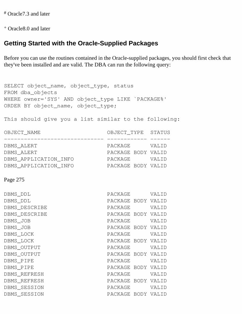
# Oracle7.3 and later
+ Oracle8.0 and later
Getting Started with the Oracle-Supplied Packages
Before you can use the routines contained in the Oracle-supplied packages, you should first check that they've been installed and are valid. The DBA can run the following query:
SELECT object_name, object_type, statusFROM dba_objectsWHERE owner='SYS' AND object_type LIKE `PACKAGE%'ORDER BY object_name, object_type;
This should give you a list similar to the following:
OBJECT_NAME OBJECT_TYPE STATUS------------------------------ ------------ ------DBMS_ALERT PACKAGE VALIDDBMS_ALERT PACKAGE BODY VALIDDBMS_APPLICATION_INFO PACKAGE VALIDDBMS_APPLICATION_INFO PACKAGE BODY VALID
Page 275
DBMS_DDL PACKAGE VALIDDBMS_DDL PACKAGE BODY VALIDDBMS_DESCRIBE PACKAGE VALIDDBMS_DESCRIBE PACKAGE BODY VALIDDBMS_JOB PACKAGE VALIDDBMS_JOB PACKAGE BODY VALIDDBMS_LOCK PACKAGE VALIDDBMS_LOCK PACKAGE BODY VALIDDBMS_OUTPUT PACKAGE VALIDDBMS_OUTPUT PACKAGE BODY VALIDDBMS_PIPE PACKAGE VALIDDBMS_PIPE PACKAGE BODY VALIDDBMS_REFRESH PACKAGE VALIDDBMS_REFRESH PACKAGE BODY VALIDDBMS_SESSION PACKAGE VALIDDBMS_SESSION PACKAGE BODY VALID

DBMS_SHARED_POOL PACKAGE VALIDDBMS_SHARED_POOL PACKAGE BODY VALIDDBMS_SNAPSHOT PACKAGE VALIDDBMS_SNAPSHOT PACKAGE BODY VALIDDBMS_SPACE PACKAGE VALIDDBMS_SPACE PACKAGE BODY VALIDDBMS_SQL PACKAGE VALIDDBMS_SQL PACKAGE BODY VALIDDBMS_SYSTEM PACKAGE VALIDDBMS_SYSTEM PACKAGE BODY VALIDDBMS_TRANSACTION PACKAGE VALIDDBMS_TRANSACTION PACKAGE BODY VALIDDBMS_UTILITY PACKAGE VALIDDBMS_UTILITY PACKAGE BODY VALID
There will be some other packages not shown here, but we won't be concerning ourselves with them. Most of these additional packages are not intended to be called by user applications, but rather are for internal use only.
Locating the DBMS Packages
The Oracle-supplied packages are located in <ORACLE_HOME>\RDBMS<version>\ADMIN where ORACLE_HOME is the path to the Oracle Home directory (you can check the system variable of the same name in UNIX or check the Registry entry under Windows 95/NT). version is the database version you are running. You can examine the package header files listed in Table 12.1 for each of these packages to see what routines and global variables are available.
You may also note the existence of files of the form prvt*.sql and prvt*.plb (for example, prvtpipe.sql and prvtpipe.plb). The former are the package bodies for the supplied packages, in ASCII format. The latter are binary compiled versions of the package body. The PLB files are recognizable by the PL/SQL engine and result in a valid and executable package body when submitted to the Oracle Server. These represent the "release" form of the package bodies.
Previous | Table of Contents | Next

Previous | Table of Contents | Next
Page 270
At the time I wrote this, I really had a weak understanding of the data dictionary views. After analyzing and playing around with them, creating objects and then seeing what the different results were, I really gained an appreciation for them. My enthusiasm level was very high after completing this project. It really made me think. The DDL syntax for many of these database objects is very rich and complex. In order to understand how constraints work, and how the rev_pkeys, rev_ukeys, rev_fkeys, and rev_checks procedures work, create these constraints and see what data is stored in dba_constraints (the constraint name and type), dba_cons_columns (the constraint columns), and dba_indexes (for the index and storage parameters).
Some issues not implemented are how to handle disabled constraints (the storage parameters for the related index are blank, which is really a syntax error— you have to add them manually), clusters (not done), tablespaces (not done), users (not done), and so on.
I've found this a very handy utility, especially for old legacy applications whose DDL files have long been deleted or outdated. I encourage you to examine it, try it, and hopefully take something from it to use in your own PL/SQL masterpieces.
The last item I feel I need to point out is actually not part of the package proper, but rather follows it. The grant and synonym created for it make the package available to all.
GRANT EXECUTE ON rev_eng TO PUBLIC;CREATE PUBLIC SYNONYM REV_ENG FOR REV_ENG;
It's a very good idea to include these items here, so that you document for whom the package is intended and manage privileges locally to the module. This will save you and all following DBAs that much trouble later on.
Previous | Table of Contents | Next

Previous | Table of Contents | Next
Page 267
when I wish to default the parameter to NULL in order to specify a "don't care" value for this column. If the parameter value is supplied, the WHERE clause will match on it; otherwise, the column is effectively ignored, for the purpose of matching.
The cursor get_constraints is actually used by all the constraint routines that need to check for the constraint type, so I gained some coding efficiency here. I generalized the cursor just enough to avoid having to declare various flavors of what's essentially the same cursor. Cursors are probably one of your bigger memory hogs. The cursor get_index_params also falls into the reuse bin. I broke out this information into a separate cursor, even though I could have shoved it messily into another, because it was cleaner this way. In general, I think I avoided joins because the underlying data dictionary tables are difficult to decipher. Try looking at the Explain Plans for some of the dba_* views. Besides, they're potentially more flexible as separate objects, which enables me to combine them as needed in nested loops.
Below the cursor declarations are the global, private variables. The known_indexes PL/SQL table stores the names of all indexes you have already processed. The known_indexes array can be cleared using the clear_indexes array by simply assigning clear_indexes to known_indexes.
known_indexes := clear_indexes; -- clear table (7.2)known_indexes.DELETE; -- clear table (7.3)
You never assign values to the elements of clear_indexes. It is always left empty. This is the standard method of clearing a PL/SQL table in Oracle7.2. In Oracle7.3, you can use the PL/SQL table attribute DELETE to clear all elements.
In order to simplify existence checks for the index presently being examined, I wrote the function idx_already_rev. Since the only way to check the array for an index name is to loop through all its entries, this function hides this implementation detail in an easy-to-use manner, as with:
IF (idx_already_rev(get_indexes_rec.index_name)) THEN GOTO SKIPIT; -- index was already reverse engineered END IF;
which is pretty readable.
Due to a bug between SQL*Plus and DBMS_OUTPUT in Oracle7.2 that causes leading whitespace to be trimmed, I use tabs heavily for indentation. A variety of character constants help me in this endeavor.

NOTE
In Oracle7.3 and later, use set serveroutput on format wrapped to prevent leading whitespace from being trimmed.
I created a date-formatting string because I write out the date everywhere, and this was a decent code reducer. If you wanted to change the date format, you only need to do it in one place.
-- declare global constant data CR CONSTANT VARCHAR2(1) := CHR(13); -- carriage return character... DFORMAT CONSTANT VARCHAR2(20) := `DD-MON-YYYY HH:MI:SS'; -- date format
Page 268
-- declare global data status NUMERIC;...-- record variables get_tables_rec get_tables%ROWTYPE;...
These global private variables were added here instead of within procedures because, again, I never knew where I'd actually use them, and some I use in more than one subprogram. Also, it was a helpful organizational aid; I could see how far along I'd gotten with the implementation by checking these, especially the cursor record variables. I only defined them as I went along, instead of trying to enumerate them all up front.
The private local routine get_parent_table is a "helping" routine used further down. It's up here and not inside the one procedure that calls it because, again, I didn't know beforehand where it might be used. The most annoying thing is to overly restrict yourself and then be forced to move chunks of code around the module. This routine uses an implicit cursor so I can detect the TOO_MANY_ROWS exception.
Note that all the exception handler sections have similar coding constructs. I always follow the same general method for writing exception handlers. I trap the error, display or store it, clean up potentially open cursors, and set any return values to default values.
EXCEPTION

WHEN OTHERS THEN BEGIN status := SQLCODE; DBMS_OUTPUT.put_line(`-- rev_indexes ERROR: ` || SQLERRM(status)); IF (get_index_cols%ISOPEN) THEN CLOSE get_index_cols; END IF; IF (get_indexes%ISOPEN) THEN CLOSE get_indexes; END IF; EXCEPTION WHEN OTHERS THEN NULL; -- don't care END; END rev_indexes;
The displayed error message is printed as a comment because I intended the programs' output to be spooled to a file and I didn't want to muck it up with stuff the user might have to cut out to get the resulting SQL file to run. Each exception handler tells you what its name is for easier debugging. Return values, if any, are set to NULL. Any cursors that might be open are closed. The entire exception handler is placed in its own block to avoid a potential infinite loop on any operation done inside the exception handler.
I wound up having to write put_long_line because of a line length limitation with DBMS_OUTPUT, particularly when printing the long text for views. It seemed like such a generally useful thing, so I made it public. This routine looks for suitable places to break long lines. I think I must have coded it five times over before I handled every situation correctly. And lest you think me
Page 269
less than analytical, I wrote out all the cases and logic on paper (also five times)! Sometimes, it's easy to miss things. Actually, the cases became more refined and the logic more concise with repetition.
TIP
For complex, difficult code pieces, it's a good idea to write out on paper beforehand all the cases and logic goals before attempting a coding solution. Then exercise the algorithm on paper to see if you missed anything.
Designing the Procedures

Turns out most of the main routines have similar elements suitable for a cut and paste operation, especially with things like converting strings to uppercase and storing in local variables.
Lowner dba_tables.owner%TYPE; Ltspace dba_tables.tablespace_name%TYPE; Ltable dba_tables.table_name%TYPE; BEGIN status := 0; Lowner := UPPER(Powner); Ltspace := UPPER(Ptspace); Ltable := UPPER(Ptable);
Note that status is a global private variable and thus it must be initialized in each routine. I've found from other projects that I might want to test certain variables in places other than in the most obvious, inside the procedures using them, so historically I've always defined status this way. Old habits die hard. When I start fleshing out a new package, I add in early the common elements I know I'll need. That's why they wind up being global private items. This way, I can test the value of status outside of any of the procedures that modify it. It's guaranteed to be available to all routines without having to remember to declare it everywhere.
The comment headers for each subprogram, and therefore each DDL statement generated, are printed with the following code:
IF (Ltable IS NULL) THEN -- parameter comments DBMS_OUTPUT.put(`-- ALL TABLES'); ELSE DBMS_OUTPUT.put(`-- TABLE ` || Ltable); END IF; DBMS_OUTPUT.put_line(` FOR OWNER ` || Lowner || `, TABLESPACE ` || Ltspace); DBMS_OUTPUT.put_line(`-- PERFORMED ` || TO_CHAR(SYSDATE, DFORMAT));
This stuff was added late in the game, and required modification of every procedure, but it was really a no-brainer after setting up the pattern.
Wrapping Up the Package
This package makes heavy use of the DBA data dictionary views for tables, indexes, constraints, views, etc. I chose the DBA views so that users could reverse-engineer any schema, not just their own or ones they have privileges on. This was especially important because an index, foreign key reference, or grant

might be made by a user other than the schema owner.
Previous | Table of Contents | Next

Previous | Table of Contents | Next
Page 276
CAUTION
Do not attempt to modify the package body of any of the Oracle-supplied packages for recompilation. You're liable to break something.
Making Sure the Packages Are Installed Correctly
You'll want to verify two things:
● The packages exist and are valid (as shown by the previous query). ● Users have EXECUTE privilege on them or the ones they intend to use.
A user can check to see if they have EXECUTE privilege on the Oracle supplied packages with the following query:
SELECT table_name, granteeFROM all_tab_privsWHERE grantor='SYS' and privilege='EXECUTE'ORDER BY table_name;
A typical response might be
TABLE_NAME GRANTEE------------------------------ ------------------------------DBMS_APPLICATION_INFO PUBLICDBMS_DDL PUBLICDBMS_DESCRIBE PUBLICDBMS_JOB PUBLICDBMS_OUTPUT PUBLICDBMS_PIPE PUBLICDBMS_SESSION PUBLICDBMS_SNAPSHOT PUBLICDBMS_SPACE PUBLICDBMS_SQL PUBLICDBMS_STANDARD PUBLICDBMS_TRANSACTION PUBLICDBMS_UTILITY PUBLICDBMS_REFRESH PUBLICUTL_FILE PUBLIC
All of the Oracle-supplied packages should have been granted with EXECUTE to PUBLIC. I used the all_flavor of the data dictionary view to verify this. If any are missing that you intend to use, the DBA can run the appropriate script as

SYS. If a package exists but is invalid, the DBA can recompile it with:
ALTER PACKAGE SYS.<name> COMPILE PACKAGE;
Where name is the name of the invalid package. The clause COMPILE PACKAGE tells Oracle to recompile the package specification and body. If just the body needs to be recompiled, instead run:
ALTER PACKAGE SYS.<name> COMPILE BODY;
Page 277
CAUTION
Some supplied packages may have dependencies on other packages. If you have to recompile a package header, this invalidates any dependent packages. Check again that other packages are still valid after recompiling. If only the body is recompiled, dependent packages are not invalidated. Any user-written stored subprograms and packages may also likely be affected in this manner.
Hands-On with the Oracle-Supplied Packages
Now for the fun part! I'll illustrate some of the more interesting contents of each supplied package with some reasonably simple and useful examples.
Monitoring Programs with DBMS_APPLICATION_INFO
This package enables developers to add application tracking information in the views v$sqlarea and v$session. The kind of data that can be tracked is
● A module name (such as the name of the currently running application), a VARCHAR2 string up to 48 bytes, stored in v$sqlarea.module and v$session.module.
● The current action (for example, "Update Customer Info," "Verify Credit Limit"), a VARCHAR2 string up to 32 bytes, stored in v$sqlarea.action and v$session.action.
● Any client-specific information, a VARCHAR2 string up to 64 bytes, stored in v$session.client_info.
Oracle doesn't do anything with this information; it's provided for the use of the DBA so he or she can run statistics against each application and component operations. Strings longer than what's supported are truncated. Listing 12.1 shows a simple example.
Listing 12.1 appinfo.sql—Setting and Reading Application Information
DECLARE module VARCHAR2(48); -- application info action VARCHAR2(32); client VARCHAR2(64); ldate VARCHAR2(30); -- to capture system dateBEGIN

DBMS_OUTPUT.enable; module := `CLAIM TRACKING'; action := `VERIFY ELIGIBILITY'; DBMS_APPLICATION_INFO.set_module(module, action); DBMS_APPLICATION_INFO.set_client_info(USER); DBMS_APPLICATION_INFO.read_module(module, action); DBMS_APPLICATION_INFO.read_client_info(client); DBMS_OUTPUT.put_line(client || ` is running ` || module || `: ` || action);
continues
Page 278
Listing 12.1 Continued
SELECT TO_CHAR(SYSDATE, `YYYY-MON-DD HH:MI:SS') INTO ldate FROM DUAL;END;/
The response I get is
SCOTT is running CLAIM TRACKING: VERIFY ELIGIBILITY
While this session is still up, the DBA can check who is doing what with:
COLUMN module FORMAT A20COLUMN action FORMAT A20COLUMN client_info FORMAT A20SELECT client_info, module, actionFROM v$sessionWHERE client_info IS NOT NULL;
To get:
CLIENT_INFO MODULE ACTION-------------------- -------------------- --------------------SCOTT CLAIM TRACKING VERIFY ELIGIBILITY
The DBA can then see the effects of everyone running this module and action with:
SELECT sql_text, SUM(sharable_mem) smem, SUM(persistent_mem) pmem, SUM(runtime_mem) rmem, SUM(sorts) sorts, SUM(loads) loads, SUM(disk_reads) rdisk, SUM(buffer_gets) bget, SUM(rows_processed) prowsFROM v$sqlareaWHERE module = `CLAIM TRACKING' AND action = `VERIFY ELIGIBILITY'

GROUP BY sql_text;
The results are pretty interesting:
SQL_TEXT------------------------------------------------------------------------------ SMEM PMEM RMEM SORTS LOADS RDISK BGET PROWS-------- -------- -------- -------- -------- -------- -------- --------SELECT TO_CHAR(SYSDATE,'YYYY-MON-DD HH:MI:SS') FROM DUAL 4267 508 792 0 1 0 4 2
SELECT USER FROM SYS.DUAL 3596 508 688 0 1 0 4 1
begin dbms_output.get_lines(:lines, :numlines); end; 4317 592 420 0 1 0 0 1
The only query I explicitly made was the first one, but SQL*Plus apparently does some work behind the scenes.
Page 279
As a module performs different actions, the developers should make the appropriate calls to set_action() to reflect this. In this manner, you can collect some interesting statistics on how badly an application is battering the server by query, by action, by module, by user, or by groups of users.
NOTE
Even after a user disconnects, entries still exist in v$sqlarea until the related SQL gets aged out of the SGA.
Recompiling Packages with DBMS_DDL
There are precisely two things you can do with this package:
● Recompile stored subprograms and packages with alter_compile(). ● Analyze a table, index, or cluster with analyze_object().
A simple use for alter_compile() would be to find what stored program objects are invalid and then recompile them. Listing 12.2 illustrates this.
Listing 12.2 recompil.sql—Recompile Invalid Program Objects Only
-- recompile invalid stored program objects-- CAVEAT: does not take package dependencies-- into account!DECLARE CURSOR invalid_prog_obj IS

SELECT object_name, object_type FROM user_objects WHERE status = `INVALID'; rec invalid_prog_obj%ROWTYPE; status NUMERIC;BEGIN DBMS_OUTPUT.enable; OPEN invalid_prog_obj; LOOP -- recompile each stored program object FETCH invalid_prog_obj INTO rec; EXIT WHEN invalid_prog_obj%NOTFOUND; DBMS_OUTPUT.put(`Recompile ` || rec.object_type || ` ` || rec.object_name); DBMS_DDL.alter_compile(rec.object_type, NULL, rec.object_name); DBMS_OUTPUT.put_line(` SUCCESSFUL'); -- recompile succeeded END LOOP; -- invalid program objects CLOSE invalid_prog_obj;EXCEPTIONWHEN OTHERS THEN BEGIN status := SQLCODE; DBMS_OUTPUT.put_line(` FAILED with ` || SQLERRM(status)); IF (invalid_prog_obj%ISOPEN) THEN CLOSE invalid_prog_obj; END IF;
continues
Previous | Table of Contents | Next

Previous | Table of Contents | Next
Page 280
Listing 12.2 Continued
EXCEPTION WHEN OTHERS THEN NULL; -- do nothing END;END;/
This might return something similar to the following:
Recompile FUNCTION TABLE_EXISTS SUCCESSFUL1 Program Objects RecompiledPL/SQL procedure successfully completed.
CAUTION
If a program object fails to recompile successfully, alter_compile will not tell you! After running alter_compile, you should check the status of the package to make sure it compiled successfully.
If you provide a program object name that doesn't exist, or you have the type wrong, you get:
ORA-20000: Unable to compile PACKAGE "BLICK", insufficient privileges or doesnot exist
You can programmatically analyze (generate statistics) for tables, indexes, and clusters. For example, you could analyze all or selected objects in your schema, as shown in Listing 12.3.
Listing 12.3 runstats.sql—Running Statistics Programmatically
-- analyze all tables, indexes and clusters in your own schema-- computes exact statisticsSET ECHO OFFACCEPT method PROMPT ` ANALYZE Method ([COMPUTE]|ESTIMATE|DELETE): `ACCEPT estrow PROMPT ` IF ANALYZE Method is ESTIMATE, #Rows (0-n)

[100]: `ACCEPT estpct PROMPT ` IF ANALYZE Method is ESTIMATE, %Rows (0-99) [20]: `DECLARE -- application-defined exceptions bad_method EXCEPTION; -- user entered an invalid method bad_estrow EXCEPTION; -- user entered an invalid est. #rows bad_estpct EXCEPTION; -- user entered an invalid est. %rows -- cursors CURSOR analyze_obj IS SELECT object_name, object_type FROM user_objects WHERE object_type = ANY (`TABLE', `INDEX', `CLUSTER'); -- constants METHOD CONSTANT VARCHAR2(30) := NVL(UPPER(`&&method'), `COMPUTE'); -- variables estrow NUMBER := NVL(`&&estrow', `100'); -- user input est. #rows estpct NUMBER := NVL(`&&estpct', `20'); -- user input est. pct
Page 281
rec analyze_obj%ROWTYPE; status NUMERIC := 0; cnt NUMERIC := 0;BEGIN DBMS_OUTPUT.enable; -- validate user input IF (METHOD NOT IN (`COMPUTE', `ESTIMATE', `DELETE')) THEN RAISE bad_method; ELSIF (METHOD IN (`COMPUTE', `DELETE')) THEN -- ignore est. #/%row estrow := NULL; estpct := NULL; ELSE -- picked ESTIMATE; must provide either est. #rows or %rows IF (estrow < 1 AND estpct = 0) THEN RAISE bad_estrow; ELSIF (estpct NOT BETWEEN 1 AND 99) THEN RAISE bad_estpct; END IF; END IF; -- validate input
OPEN analyze_obj; LOOP -- analyze schema objects FETCH analyze_obj INTO rec;

EXIT WHEN analyze_obj%NOTFOUND; -- COMPUTE STATISTICS for this schema only DBMS_OUTPUT.put(`Analyze ` || METHOD || ` ` || rec.object_type || ` ` || rec.object_name); DBMS_DDL.analyze_object(rec.object_type, NULL, rec.object_name, `COMPUTE'); DBMS_OUTPUT.put_line(` SUCCESSFUL'); cnt := cnt + 1; END LOOP; -- analyze schema objects CLOSE analyze_obj; DBMS_OUTPUT.put_line(TO_CHAR(cnt) || ` objects analyzed');
EXCEPTIONWHEN bad_method THEN DBMS_OUTPUT.put_line(`Invalid Method! Must be COMPUTE, ESTIMATE orDELETE only');WHEN bad_estrow THEN DBMS_OUTPUT.put_line(`Invalid Est. #Rows! Must be >= 1');WHEN bad_estpct THEN DBMS_OUTPUT.put_line(`Invalid Est. %Rows! Must be between 1 and 99');WHEN OTHERS THEN BEGIN status := SQLCODE; DBMS_OUTPUT.put_line(` FAILED with ` || SQLERRM(status)); IF (analyze_obj%ISOPEN) THEN CLOSE analyze_obj; END IF; EXCEPTION WHEN OTHERS THEN NULL; END;END;/
Page 282
Note all the input validation we have to do. Partly, this is because analyze_object does very little of its own. If you provided a row estimate along with the COMPUTE method, for instance, you'll get:
Analyze TABLE <table> FAILED with ORA-01490: invalid ANALYZE command.
When I compute statistics by picking all the defaults, my run looks like this:

ANALYZE Method ([COMPUTE]|ESTIMATE|DELETE): IF ANALYZE Method is ESTIMATE, #Rows (1-n) [1]: IF ANALYZE Method is ESTIMATE, %Rows (1-99) [20]:old 12: METHOD CONSTANT VARCHAR2(30) := NVL(UPPER(`&&method'), `COMPUTE');new 12: METHOD CONSTANT VARCHAR2(30) := NVL(UPPER(`'), `COMPUTE');old 14: estrow NUMBER := NVL(`&&estrow', `1'); -- user input est. #rowsnew 14: estrow NUMBER := NVL(`', `1'); -- user input est. #rowsold 15: estpct NUMBER := NVL(TRUNC(`&&estpct'), `20'); -- user input est. pctnew 15: estpct NUMBER := NVL(TRUNC(`'), `20'); -- user input est. pctAnalyze COMPUTE TABLE BONUS SUCCESSFULAnalyze COMPUTE TABLE DEPT SUCCESSFULAnalyze COMPUTE TABLE EMP SUCCESSFULAnalyze COMPUTE INDEX PK_DEPT SUCCESSFULAnalyze COMPUTE INDEX PK_EMP SUCCESSFULAnalyze COMPUTE TABLE SALGRADE SUCCESSFUL6 objects analyzedPL/SQL procedure successfully completed.
If you enter in an invalid method, it complains with:
Invalid Method! Must be COMPUTE, ESTIMATE or DELETE only
as we desired. Play around with it and see how you like it.
This implementation of the ANALYZE command doesn't do VALID STRUCTURE or LIST CHAINED ROWS. In this respect, it's an incomplete implementation, but it's still pretty useful.
Formatting Output with DBMS_OUTPUT
If you've been following along since the tutorial, you're already familiar with the put_line procedure in this package. Here are some details regarding the implementation of the package:
● Each line is terminated with a newline character. ● Each line may only be up to 255 bytes, including the newline character. ● Each line is stored in a private PL/SQL table. ● Nothing is stored unless DBMS_OUTPUT.ENABLE is first called. ● The buffer size specified must be in the range 2,000 to 1,000,000.

You use the procedure enable to turn on the output feature. put_line calls are ignored if output hasn't first been enabled. When you enable output, you can also specify a buffer size, as with:
DBMS_OUTPUT.enable(1000000); -- 1 million bytes is the max
Page 283
Conversely, you can turn output back off with disable:
DBMS_OUTPUT.disable; -- turn off output
You can store a line of text with put_line. It's overloaded to take a DATE, NUMBER or VARCHAR2. You can also store a line of text without terminating it by using the put procedure (which is overloaded in like manner). This is useful if the line you're building requires some logic:
-- excerpt taken from Package rev_engIF (Ltable IS NULL) THEN -- parameter comments
DBMS_OUTPUT.put(`-- ALL TABLES');ELSE DBMS_OUTPUT.put(`-- TABLE ` || Ltable);END IF;DBMS_OUTPUT.put_line(` FOR OWNER ` || Lowner || `, TABLESPACE ` || Ltspace);
You can terminate text submitted with put by using the new_line procedure. This signals the end of the current line of text with a marker, and also stores the length of the text line along with the text (this is completely transparent to the user). Note that if you try to double or triple space output lines by sending new lines without first using put, it doesn't work:
BEGIN DBMS_OUTPUT.put(`Hey, `); DBMS_OUTPUT.put(`Dan!'); DBMS_OUTPUT.new_line; DBMS_OUTPUT.new_line; DBMS_OUTPUT.put_line(`Time to go Hot Tubbing!');end;
Gives you:
Hey, Dan!

Time to go Hot Tubbing!PL/SQL procedure successfully completed.
It didn't double space. Oh well.
You'll get an exception if you attempt to output a string longer than the acceptable 255 bytes before ending it with new_line:
ORA-20000: ORU-10028: line length overflow, limit of 255 bytes per line.
Why did the folks at Oracle limit the string length to 255? Look back to the example where a PL/SQL table of VARCHAR2 (32767) quickly exhausted available memory (see Chapter 10, "PL/SQL Fundamentals," Listing 4.10). So they picked what they considered a reasonable limit.
Strings are returned with get_line. This is what SQL*Plus does to return the strings written with put_line. Unseen, it calls get_line until no more lines are available. You really only need concern yourself with get_line (and its multiple line version, get_lines) if you're writing a 3GL program to receive lines stored with put_line. You can use it in a PL/SQL program if you wish, such as to buffer lines and then access them in FIFO manner, perhaps to insert them into a table.
Previous | Table of Contents | Next

Previous | Table of Contents | Next
Page 305
Chapter 13
Import/Export
In this chapter
● Understanding the Purpose and Capabilities of Import/Export 306 ● Understanding Behavior 307 ● Controlling and Configuring Import and Export 309 ● Taking Walkthroughs of Import and Export Sessions 319 ● Using the SHOW and INDEXFILE Options 326
Page 306
Understanding the Purpose and Capabilities ofImport/Export
The Oracle8 Server comes with two important utilities: Import and Export. These two utilities are useful for many important database functions such as backing up data, copying objects among different schemas and databases, and generating object creation scripts. They are also useful in migrating from one version of Oracle to another, and may be used to upgrade your database to Oracle8.
The Import and Export utilities provide a wide range of capabilities. The main purpose is to back up and recover data and objects. The objects and data are stored in a binary form that may be read only by Oracle databases. Export and Import can perform the following tasks:
● Back up and recover your databases.Export and Import are frequently used as part of a backup plan. Typically, full or hot backups are used to back up the entire database in the event of a disk or computer failure. However, if just one table in the entire database needs to be recovered, the entire database would have to be recovered on another machine, and the one table would be copied over. This is incredibly time and resource consuming. Import and Export can save you this hassle by providing the capability to export the entire database and import just the tables you need recovered. They may also serve as a backup and recovery mechanism for the entire database, because Point-in-time Recovery is also an option.
● Move data and objects among schemas.

You can use Import and Export to copy tables, indexes, grants, procedures, and views, among all other object types from one schema to another. This helps save time and effort because you can just specify those objects you desire to move. Also, moving data may be used as a form of data replication among different Oracle databases.
● Migrate databases from one Oracle version to another.You can upgrade (or downgrade) the version of Oracle by using the Import and Export utilities. You can export an entire Oracle7 database, for example. Then, providing you have the Oracle8 Server installed, the database can be imported, making the data and application function in an Oracle8 environment. This process is called migration.
● Defragment a tablespace or the entire database.Fragmentation occurs when objects such as tables and indexes are created, deleted, enlarged, and reduced in size over time. Fragmentation also occurs when object storage parameters are poorly defined. By exporting a tablespace, coalescing space, and importing objects again, you can defragment tablespaces.
● Generate CREATE scripts.You can also use Import and Export to generate CREATE scripts for tables, partitions, views, grants, indexes, constraints, and tablespaces, among all other objects in the database. This proves quite useful for modifying objects and safeguarding the structure of your objects in the event one gets corrupted or deleted.
Page 307
NOTE
The export file is in a binary format that may only be used with Oracle databases. You cannot export from Oracle and import into a non-Oracle database. Similarly, you cannot import from a non-Oracle database. If you wish to copy data to Oracle from another database product such as Microsoft Access, you should use SQL*Loader on a delimited file format of the data, such as CSV (comma-separated values). To transfer data from Oracle to a non-Oracle database, you must make a delimited file manually by spooling from within PL/SQL or SQL*Plus.
Understanding Behavior
There are three types of exports:
● FULL export: Exports all objects, structures, and data within the database. ● OWNER export: Exports only those objects owned by a particular user account. ● TABLE export: Exports only the specified tables and partitions.
With dozens of types of structures that may be exported, it is important to distinguish what gets exported with each of the three export categories. Table 13.1 shows which structures are exported with each

export option (in the order that Export exports). The following section then describes the syntax of running exp80 and imp80, executables for export and import with Oracle8.
NOTE
In a Windows NT environment, exp80 and imp80 are the commands for the Export and Import utilities. On UNIX and other operating systems, exp and imp are the commands for the Export and Import utilities. For simplicity, this book provides all examples with the xp80 and imp80 commands.
Table 13.1What Objects Get Exported with Each of the Three Export Options
Type of Object
with FULL=Y option
with OWNER option
with TABLEoption
Tablespacedefinitions
All objects
Profiles All objects
Userdefinitions
All objects
Roles All objects
Resource costs
All objects
continues
Page 308
Table 13.1Continued
Type of Object with FULL=Y option with OWNER option with TABLEoption Rollbacksegmentdefinitions All objects Database links All objects Just for owner Sequence numbers All objects Just for ownerDirectory aliases All objectsForeignfunctionlibrary names All objects Just for owner Object typedefinitions All objects Just for ownerCluster definitions All objects Just for owner Just for table

and owner Tables All objects Just for owner Just for table andowner Indexes All objects Just for owner Just for table andowner Referentialintegrityconstraints All objects Just for owner Just for tableand ownerPostable actions All objects Just for owner Synonyms All objects Just for owner Just for table andowner Views All objects Just for owner Stored procedures All objects Just for ownerTriggers All objects Just for owner Just for table andowner Snapshots All objects Just for owner Snapshot logs All objects Just for owner Job queues All objects Just for owner
Previous | Table of Contents | Next

Previous | Table of Contents | Next
Page 304
Moving right along, let's find out what platform we're running:
EXECUTE DBMS_OUTPUT.put_line(DBMS_UTILITY.port_string);
I get:
IBMPC/WIN_NT-7.3.3
What do you get?
I've touched upon the most readily usable packaged subprograms provided by Oracle. By using these routines, you can accomplish quite a bit more programmatically than you may have been used to. I encourage you to try them on your own, and to also examine some of the others (like DBMS_ALERT) not delved into in this section. Your ability to tune the database and applications should improve with their use.
Previous | Table of Contents | Next

Previous | Table of Contents | Next
Page 299
Here's a sample run:
Enter Username: scottTurn Trace ON/OFF: onold 8: OWNER CONSTANT VARCHAR2(30) := UPPER(`&&owner');new 8: OWNER CONSTANT VARCHAR2(30) := UPPER(`scott');old 9: SETTRACE CONSTANT VARCHAR2(3) := RTRIM(UPPER(`&&trace'));new 9: SETTRACE CONSTANT VARCHAR2(3) := RTRIM(UPPER(`on'));TRACE FOR USER SCOTT is now ONPL/SQL procedure successfully completed.
Once turned on, the trace remains active until you or the user turns trace back off, or the user disconnects.
Using Miscellaneous Utilities in DBMS_UTILITY
This package contains a bunch of useful routines, some of which I'll illustrate. A brief description of them is given in Table 12.3.
Table 12.3 Miscellaneous Utility Routines Found in DBMS_UTILITY
Subprogram Description
PROCEDURE compile_schema( Powner VARCHAR2);
Recompiles all stored subprograms and packages in a given schema.
PROCEDURE analyze_schema( Powner VARCHAR2, Pmethod VARCHAR2, Pest_rows NUMBER DEFAULT NULL, Pest_pct NUMBER DEFAULT NULL);
Performs ANALYZE on all tables, indexes, and clusters for the given schema.
FUNCTION format_error_stack RETURN VARCHAR2;
Returns a string containing the first 2,000 bytes of the error stack.

FUNCTION format_call_stack RETURN VARCHAR2;
Returns a string containing the first 2,000 bytes of the program call stack.
FUNCTION is_parallel_server RETURN BOOLEAN;
Returns TRUE/FALSE indicating whether parallel option for this server is turned on.
FUNCTION get_time RETURN NUMBER;
Returns the time in hundredths of a second since the epoch (good for timing applications).
continues
Page 300
Table 12.3 Continued
Subprogram Description
PROCEDURE name_resolve( Pname IN VARCHAR2, Pcontext IN NUMBER, Powner OUT VARCHAR2, Ppart1 OUT VARCHAR2, Ppart2 OUT VARCHAR2, Plink OUT VARCHAR2, Ppart1_type OUT NUMBER, Pobj_number OUT NUMBER);
Resolves a given object name, expanding synonyms and following remote database links as necessary; also does authorization checking.
PROCEDURE name_tokenize( Pname IN VARCHAR2, Powner OUT VARCHAR2, Ptable OUT VARCHAR2, Pcol OUT VARCHAR2, Plink OUT VARCHAR2, Pnext OUT BINARY_INTEGER);
Given a string containing an object reference in dot notation, breaks it up into its component parts: owner, table, column, database link.

PROCEDURE comma_to_table( Plist IN VARCHAR2, Ptabn OUT BINARY_INTEGER, Ptab OUT uncl_array);
Given a string containing tokens separated by commas, loads the tokens into a PL/SQL table, starting with table element 1.
PROCEDURE table_to_comma( Ptab IN uncl_array, Ptabn OUT BINARY_INTEGER, Plist OUT VARCHAR2);
Given a PL/SQL table, builds a comma-delimited string consisting of the values from the table. The first table element must be 1 and the last table entry must be NULL.
FUNCTION port_string RETURN VARCHAR2;
Returns a string containing the version of Oracle and the operating system.
FUNCTION make_data_block_address( Pfile NUMBER, Pblock NUMBER) RETURN NUMBER;
Given a file and block number, returns the data block address; used for accessing fixed tables containing data block addresses.
FUNCTION data_block_address_file( Pdba NUMBER) RETURN NUMBER;
Given a data block address, returns the file portion of it.
Page 301
Subprogram Description

FUNCTION data_block_address_block( Pdba NUMBER) RETURN NUMBER;
Given a data block address, returns the data block portion of it.
You can use format_error_stack in exception handlers to display the error stack right at the point where it's most useful, perhaps storing the string in an error log table, or sending it to another session via a pipe. Here's a very simple example:
DECLARE x VARCHAR2(1);BEGIN x := `bust!';EXCEPTIONWHEN OTHERS THEN DBMS_OUTPUT.put_line(DBMS_UTILITY.format_error_stack);END;/
which returns:
ORA-06502: PL/SQL: numeric or value errorPL/SQL procedure successfully completed.
In a similar vein, you can use format_call_stack to view the calling stack. This is useful when you're nested down several levels through various subprograms. Here is a modest example (see Listing 12.13).
Listing 12.13 callstk.sql—What's on the Call Stack?
CREATE TABLE call_log ( log_date DATE, log_level NUMBER, log_msg VARCHAR2(2000))/
DECLARE x NUMBER; PROCEDURE nest(Plevel IN OUT NUMBER, Pstopat IN NUMBER) IS msg VARCHAR2(2000); BEGIN IF (Plevel < Pstopat) THEN Plevel := Plevel + 1; -- increment nesting depth

nest(Plevel, Pstopat); ELSE msg := DBMS_UTILITY.format_call_stack; INSERT INTO call_log VALUES (SYSDATE, Plevel, msg); END IF; END nest;
continues
Page 302
Listing 12.13 Continued
BEGIN x := 1; -- always start with 1 nest(x, 4);END;/
SELECT * FROM call_log ORDER BY log_date/
DROP TABLE call_log/
I get:
Table created.PL/SQL procedure successfully completed.LOG_DATE LOG_LEVEL-------- --------LOG_MSG----------------------------------------27-NOV-97 4---- PL/SQL Call Stack ---- object line object handle number name 12770c8 10 anonymous block 12770c8 8 anonymous block 12770c8 8 anonymous block 12770c8 8 anonymous block

12770c8 17 anonymous blockTable dropped. ?
Okay, so this isn't the most useful thing in an anonymous block. If you used it in a stored procedure with some sort of trace mechanism (like the one we built earlier), you could unwind the stack during a debugging session to see where your program is going.
Moving right along, let's see whether our server is running Parallel Query Mode by using Listing 12.14.
Listing 12.14 pqm.sql—Check to See if We're Running Parallel Query Mode
BEGIN DBMS_OUTPUT.enable; IF (DBMS_UTILITY.is_parallel_server) THEN DBMS_OUTPUT.put_line(`database is running in parallel server mode'); ELSE DBMS_OUTPUT.put_line(`database is NOT running in parallel server mode'); END IF;END;/
Page 303
I think I wrote this in 30 seconds, a new world record! Running it I get:
database is NOT running in parallel server modePL/SQL procedure successfully completed.
We're on a roll. Now let's do a timing example, as shown below in Listing 12.15.
Listing 12.15 timetest.sql—Loop Index Timing Test: NUMBER versus PLS_INTEGER, Which Is Faster?
-- Loop Indexing Test: NUMBER vs. PLS_INTEGERDECLARE maxnum CONSTANT NUMBER := 100000; -- number of loops to do maxbin CONSTANT PLS_INTEGER := 100000; -- number of loops to do time_start NUMBER; -- time we started (in 10ms) time_stop NUMBER; -- time we stopped (in 10ms) numloops NUMBER := 0; -- loop index

binloops PLS_INTEGER := 0; -- loop indexBEGIN DBMS_OUTPUT.enable;
time_start := DBMS_UTILITY.get_time; WHILE (numloops < maxnum) LOOP -- spin our wheels numloops := numloops + 1; END LOOP; -- spinning time_stop := DBMS_UTILITY.get_time; DBMS_OUTPUT.put_line(`Looping with NUMBER index ` || TO_CHAR(maxnum) || `x takes ` || TO_CHAR(time_stop - time_start) || ` hundredths of a sec');
time_start := DBMS_UTILITY.get_time; WHILE (binloops < maxbin) LOOP -- spin our wheels binloops := binloops + 1; END LOOP; -- spinning time_stop := DBMS_UTILITY.get_time; DBMS_OUTPUT.put_line(`Looping with PLS_BINARY index ` || TO_CHAR(maxbin) || `x takes ` || TO_CHAR(time_stop - time_start) || ` hundredths of a sec');
END;/
And I get:
Looping with NUMBER index 100000x takes 140 hundredths of a secLooping with PLS_BINARY index 100000x takes 54 hundredths of a secPL/SQL procedure successfully completed.
Wow! PLS_INTEGER math is a lot quicker.
Previous | Table of Contents | Next

Previous | Table of Contents | Next
Page 309
Type of Object
with FULL=Y option
with OWNER option
with TABLEoption
Refresh groupsand children
All objects Just for owner
User history table
All objects
Default andsystem auditingoptions
All objects
CAUTION
ROWIDs are re-assigned during an import. If a table has a column with ROWID information, the data will become obsolete. Also, ROWID snapshots become obsolete after an import and must be refreshed with the COMPLETE option before they can be automatically refreshed again. In addition, some REF attributes may contain ROWID information, so the REFs may become obsolete during an Import session. To re-create the REF information with proper ROWIDs after importing the data, issue the ANALYZE TABLE owner.table_name VALIDATE REF UPDATE; command.
Controlling and Configuring Import and Export
The Import and Export utilities—with the availability of dozens of parameters that can be passed—are extremely flexible. Also, there are two methods of running Import and Export: Interactive mode and Non-interactive mode. With the Interactive mode, you are stepped through a series of prompts to enter the basic information for an import and export session. This method is less flexible; you are prompted for only a few of the dozens of available parameters.
To export with the Interactive mode, just enter exp80 at the command line. You are then prompted for a username and password.
CAUTION

To export the entire database, the user account that you export with must have been granted the EXP_FULL_DATABASE system privilege. For accounts with DBA privileges, such as SYSTEM, this privilege is implicitly granted to the user. Otherwise, the export will fail.
Next, you receive a prompt for the array fetch buffer size. This is the size of the memory buffer through which rows are exported. This should be larger than the size of the largest record multiplied by the number of rows that you wish to fit within the buffer, and is operating-system dependent.
Page 310
You then receive a prompt for the name of the export file. By default, it is expdat.dmp. Next, a small menu with three options appears: (1)E(ntire database), (2)U(sers), or (3)T(ables).
If you select option 1, you receive a prompt to enter values for grants (Y/N), table data (Y/N), and compress extents (Y/N).
If you select option 2, you receive a prompt to enter values for grants (Y/N), table data (Y/N), compress extents (Y/N), and user(s) to be exported (keep entering until done, and then enter a single period on the line to finish).
If you select option 3, you receive a prompt to enter values for export table data (Y/N), compress extents (Y/N), and Table (T) or Partition (T:P) to be exported (keep entering until done, and then enter a single period on the line to finish).
To export in Non-interactive mode, you can either pass all parameters at the command line or through a parameter file. For all possible parameters of the export command, type exp80 help=y in Windows NT, as shown in Figure 13.1.
FIG. 13.1Sample result of exp80help=y, in a Windows NTenvironment.
You can use 23 parameters during an export session. You can either specify them in the command line or any parameter file that is specified. Table 13.2 describes all the export parameters.

Table 13.2Description of Parameters for the Export Utility
Parameter Default Value Description BUFFER
OS-Dependent
The size of BUFFER (in bytes) determines the memory buffer through which rows are exported. This should be larger than the size of the largest record multiplied by the number of rows that you wish to fit within the buffer.
Page 311
Parameter Default Value
Description
COMPRESS Y
If COMPRESS=Y, the INITIAL storage parameter will be set to the total size of all extents allocated for the object. The change takes effect only when the object is imported.
CONSISTENT N
Setting CONSISTENT=Y exports all tables and references in a consistent state. This slows the export because rollback space is used. If CONSISTENT=N, which is the default, and a record is modified during the export, the data becomes inconsistent.
CONSTRAINTS N Specifies whether table constraints are exported.

DIRECT N
If DIRECT=Y, Oracle bypasses the SQL command processing layer, improving the speed of the export. Unfortunately, the new object types endemic to Oracle8, such as LOBs, will not get exported.
FEEDBACK 0
Oracle displays a period for each group of records inserted. The size of the group is defined by FEEDBACK. By setting FEEDBACK=1000, for example, a period displays for every 1000 records imported. This parameter is useful for tracking the progress of large imports.
FILE expdat.dmp
By default, expdat.dmp (stands for EXPort DATa.DuMP) will be the name of the file. For a more meaningful file name, change the FILE parameter.
FULL N
The entire database will be exported if FULL=Y, including tablespace definitions.
GRANTS Y Specifies whether all grant definitions will be exported for the objects being exported.
HELP N
No other parameters are needed if you specify HELP=Y. A basic help screen is displayed.
continues
Page 312
Table 13.2Continued

Parameter Default Value
Description
INCTYPE
The valid options for the INCTYPE parameter are COMPLETE, CUMULATIVE, and INCREMENTAL. A COMPLETE export lays down a full export for which the other two options rely on for restores of the database. CUMULATIVE exports all tables and other objects that have changed since the last CUMULATIVE or COMPLETE export was taken. If one record in a table has been altered, the entire table is exported. INCREMENTAL exports all tables and objects that have changed since the last INCREMENTAL, CUMULATIVE, or COMPLETE export.

INDEXES Y
Specifies whether user-defined indexes are exported. System indexes created with constraints (primary key, unique key) and OID indexes are automatically exported, regardless of the value of the INDEXES parameter.
LOG
The LOG parameter specifies the name of the file to spool the feedback from the export session. Unless otherwise specified, Oracle appends a .LOG extension to the file.
PARFILE
Instead of entering all parameters on the command line, some or all may be kept in a parameter file. The PARFILE parameter specifies which file to use, if desired. This parameter is especially useful for non-interactive import sessions.

POINT_IN_TIME_RECOVER N
Exports information for a Point-in-time Recovery for the tablespace listed with the TABLESPACES parameter.
Previous | Table of Contents | Next

Previous | Table of Contents | Next
Page 313
Parameter Default Value
Description
RECORD Y
If using the INCTYPE parameter with RECORD=Y, the SYS data dictionary tables INCEXP, INCFIL, and INCVID are populated with export data such as owner, type of export, and the time of export.
RECORD_LENGTH OS-Dependent
The RECORD_LENGTH parameter is used only when you will import on a machine with a different byte count of the file than on the machine where the export occurs. In most import sessions, the default should be used.
RECOVERY_TABLESPACES
The RECOVERY_TABLESPACES, used in conjunction with the POINT_IN_TIME_RECOVER parameter, specifies which tablespaces may be recovered using Point-in-time Recovery. This is important because imports could not otherwise recover transactions past the time of export.
ROWS Y
Specifies whether table and object data will be exported. If ROWS=N, only object definitions are exported.

STATISTICS ESTIMATE
Specifies whether table and index statistics are to be analyzed with COMPUTE or ESTIMATE when imported. Note that only those objects that already have statistics on them will be analyzed during import. Specify NONE if no objects should be analyzed.
TABLES
Specifies a comma-separated list of all tables to be exported. This parameter should be used in conjunction with the FROMUSER parameter. In a non-UNIX environment, such as Windows NT, you must enclose the table list within parentheses.
Page 314
Table 13.2Continued
Parameter Default Value Description TABLESPACES List of tablespaces to be exported with the POINT_IN_TIME_RECOVER parameter. USERID Specifies the username and password for the user conducting the import. The format for the command is username/password. You may also use Net8's @connect_string format if desired.
To use Import with the Interactive mode, just enter imp80 at the command line. You then receive a prompt for a username and password.
CAUTION
To use Import from a DBA-invoked export, the user account that you import with must have been granted the IMP_FULL_DATABASE system privilege. For accounts with DBA privileges such as SYSTEM, this privilege is implicitly granted to the user. Otherwise, the import will fail.
You then receive a prompt for the name of the export file from which to import. By default, it is expdat.dmp. Next, you receive a prompt for the array fetch buffer size. This is the size of the memory buffer through which rows are exported. This should be larger than the size of the largest record multiplied by

the number of rows that you wish to fit within the buffer and is operating-system dependent.
Next, you are asked whether you want to list the contents of the import file only (Yes/No). The results if you select Yes are described later in this chapter in the section titled "Using the SHOW and INDEXFILE Options." If you select No, you are asked whether to ignore all create errors that may occur due to object existence (Yes/No). Then you are asked whether to import grants, table data, and the entire export file.
If you select No to import the entire export file, you receive a prompt for the username corresponding to the owner of the objects. This is followed by a repeating prompt to enter all tables and partitions. If you leave the line blank, all objects for the username are assumed. To stop the repeating prompt, enter a single period at the prompt.
To use Import in Non-interactive mode, you can either pass all parameters at the command line or through a parameter file. For all possible parameters of the import command, type imp80 help=y, as shown in Figure 13.2.
Page 315
FIG. 13.2Sample output fromimp80 help=y on aWindows NT platform.
You can use 24 parameters during an import session. You can specify them in either the command line or any parameter file that is specified. Table 13.3 describes all the import parameters.
Table 13.3Description of Parameters for the Import Utility
Parameter Default Value
Description

ANALYZE Y
Tables that are imported will have their statistics analyzed if ANALYZE is set to Y. Note that only those tables that already had statistics on them during the export will be computed. The tables will be ESTIMATEd by default, unless the export was performed with the STATISTICS=COMPUTE parameter configuration.
BUFFER OS-Dependent
The size of BUFFER (in bytes) determines the memory buffer through which rows are imported. This should be larger than the size of the largest record multiplied by the number of rows that you wish to fit within the buffer.
continues
Page 316
Table 13.3Continued
Parameter Default Value
Description
CHARSET
The CHARSET is an obsolete Oracle6 parameter, indicating whether the export was done in ASCII or EBCDIC. In Oracle7 and Oracle8, this information is processed automatically.
COMMIT N
By default, a commit occurs after each table, nested table, and partition. If you are importing a large table, the rollback segments may grow large. To improve performance while loading large tables, you should set COMMIT=Y.

DESTROY N
If you set DESTROY=Y and do a full import, Oracle overwrites any datafiles that exist. If you use raw devices for your datafiles, they will be overwritten during a full import because DESTROY=N will not prevent the overwriting of datafiles! It is always a good practice to back up the database before such an import. Do not use this option unless you know what you are doing.
FEEDBACK 0
Oracle displays a period for each group of records inserted. The size of the group is defined by FEEDBACK. By setting FEEDBACK=1000, for example, a period displays for every 1000 records imported. This parameter is useful for tracking the progress of large imports.
FILE expdat.dmp
By default, expdat.dmp (stands for EXPort DATa.DuMP) is the name of the file that Import will import from. If the file is something other than expdat.dmp, specify it with the FILE parameter.
FROMUSER
Specifying this parameter imports only those objects owned by the FROMUSER user account.
Previous | Table of Contents | Next

Previous | Table of Contents | Next
Page 329
CHAPTER 14
SQL*Loader
In this chapter
● Running SQL*Loader 330 ● Components of SQL*Loader 331 ● Looking at SQL*Loader Examples 333 ● Conventional and Direct Path Loading 347
Page 330
Running SQL*Loader
Databases today are ever increasing in complexity and size. Gigabyte-sized databases are common and data warehouses are often reaching the terabyte-sized range. With the growth of these databases, the need to populate them with external data quickly and efficiently is of paramount importance. To handle this challenge, Oracle provides a tool called SQL*Loader to load data from external data files into an Oracle database.
SQL*Loader has many functions that include the following capabilities:
● Data can be loaded from multiple input datafiles of differing file types. ● Input records can be of fixed and variable lengths. ● Multiple tables can be loaded in the same run. It can also logically load selected records into each
respective table. ● SQL functions can be used against input data before loading into tables. ● Multiple physical records can be combined into a single logical record. Likewise, SQL can take a
single physical record and load it as multiple logical records.
SQL*Loader can be invoked by typing in sqlload, sqlldr, or sqlldr80 at the command line. The exact command may differ, depending on your operating system. Refer to your Oracle operating system-specific manual for the exact syntax. Please note that all listings and server responses in this chapter may differ with your results based on the operating system that you are using. The sqlldr command accepts numerous command-line parameters. Invoking SQL*Loader without any parameters displays help

information on all the valid parameters (see Listing 14.1).
Listing 14.1SQL*Loader Help Information
Invoking SQL*Loader without parameters:$ sqlldrThe server responds with help information because SQL*Loader was invokedwithout parameters:
SQL*Loader: Release 8.0.3.0.0 - Production on Mon Nov 17 9:38:19 1997
(c) Copyright 1997 Oracle Corporation. All rights reserved.
Usage: SQLLOAD keyword=value [,keyword=value,...]
Valid Keywords:
userid -- ORACLE username/password control -- Control file name log -- Log file name bad -- Bad file name data -- Data file name discard -- Discard file namediscardmax -- Number of discards to allow (Default all)
Page 331
skip -- Number of logical records to skip (Default 0) load -- Number of logical records to load (Default all) errors -- Number of errors to allow (Default 50) rows -- Number of rows in conventional path bind array or between direct path data saves (Default: Conventional path 64, Direct path all) bindsize -- Size of conventional path bind array in bytes (Default 65536) silent -- Suppress messages during run (header,feedback,errors,discards,partitions) direct -- use direct path (Default FALSE) parfile -- parameter file: name of file that contains parameter specifications parallel -- do parallel load (Default FALSE)

file -- File to allocate extents fromskip_unusable_indexes -- disallow/allow unusable indexes or index partitions (Default FALSE)skip_index_maintenance -- do not maintain indexes, mark affected indexes as unusable (Default FALSE)commit_discontinued -- commit loaded rows when load is discontinued (Default FALSE)
PLEASE NOTE: Command-line parameters may be specified either byposition or by keywords. An example of the former case is `sqlloadscott/tiger foo'; an example of the latter is `sqlload control=foouserid=scott/tiger'. One may specify parameters by position beforebut not after parameters specified by keywords. For example,`sqlload scott/tiger control=foo logfile=log' is allowed, but`sqlload scott/tiger control=foo log' is not, even though theposition of the parameter `log' is correct.
Components of SQL*Loader
SQL*Loader is an Oracle utility that loads data into the database from external data files. Figure 14.1 shows the different components of SQL*Loader.
The Control File
The control file is the nerve center of SQL*Loader. This is the file that controls how data in the external data file is to be mapped into Oracle tables and columns. It should be noted that SQL*Loader input datatypes are totally independent from the database column datatypes into which they are being loaded. Implicit datatype conversions will be done as necessary and errors will be trapped if the conversion fails. The language used in the control file is the SQL*Loader Data Definition Language (DDL). The control file consists of multiple sections with many parameters, too many to cover in depth for the scope of this chapter. Refer to the Oracle Server Utilities manual for full documentation on all valid syntax and parameters of the control file. Basic syntax is covered in a later section when examples are given to demonstrate the different uses of SQL*Loader.
Page 332
FIG. 14.1SQL*Loader Components.

SQL*Loader Input Data
SQL*Loader can accept input data files in many different formats. Files can be stored on disk, tape, or the records themselves can be embedded into the control file. Record formats can be of fixed or variable lengths. Fixed-length records are records in which every record is the same fixed length and the data fields in each record have the same fixed length, datatype, and position. For example, the PART_NBR data item in a record would always occupy columns 10 to 19, regardless of the actual length of the data. If the part number were 12345, the remaining space in columns 15 to 19 would be blank. With variable-length records, the data item would only take up as much space as necessary on each record.
In the PART_NBR example, the data item would need only five bytes with no trailing blanks. Each record in a variable length formatted file may have different space usage for PART_NBR based on its actual length. It is important to note that even though variable-length records may use less space in the data file, data items on each record have to have a delimiter to separate the data items.
SQL*Loader Outputs
Oracle Tables and IndexesSQL*Loader can load multiple tables and indexes in an Oracle database in the same loader session. SQL*Loader's behavior in inserting the data and building the indexes will be discussed later in the section covering conventional and direct path loading.
Previous | Table of Contents | Next

Previous | Table of Contents | Next
Page 326
tablespace of the user. Before Oracle can import the data into TABLESPACE_B, you must give a large enough quota on the tablespace to the USER_A user. This is shown in the following step.
6. Issue "ALTER USER USER_A QUOTA UNLIMITED ON TABLESPACE_B;". By giving an unlimited quota, the import will succeed, providing that TABLESPACE_B is large enough to handle all the database objects being imported.
7. Import the database objects that were exported. By default, the Import utility attempts to import them into TABLESPACE_A. Because the user does not have a quota on that tablespace, however, the objects will be created in USER_A's default tablespace TABLESPACE_B.
The preceding steps show how you can use the Import and Export utilities, along with knowledge of SQL, to do powerful operations on data with relative ease. One of the most useful capabilities of the Import and Export utilities is the use of the SHOW and INDEXFILE options, as described in the following section.
Using the SHOW and INDEXFILE Options
You can use the SHOW parameter to generate all SQL statements used to create the database structure and all objects. This includes creating comments, tablespaces, users, privilege grants, roles and their assignments, quota definitions, rollback segments, sequences, tables, constraints, indexes, packages, procedures, partitions, user-defined datatypes, and so on.
One powerful use of the SHOW parameter is to create a script file that can re-create part or all of the database. The statements are listed in the proper order of dependencies—that is, a table is created before an index, a foreign key that references a primary key is created after the primary key, and so on. Listing 13.3 shows a sample portion of the output from specifying SHOW=Y.
Listing 13.3CHP13_3.lst—Sample Portion of Importing with the SHOW=Y Specification
"ALTER SCHEMA = "QUE"" "CREATE UNIQUE INDEX "I_PRICE" ON "PRICE" ("PRODUCT_ID" , "START_DATE" ) PC" "TFREE 10 INITRANS 2 MAXTRANS 255 STORAGE (INITIAL 10240 NEXT 10240 MINEXTEN" "TS 1 MAXEXTENTS 121 PCTINCREASE 50 FREELISTS 1) TABLESPACE "USER_DATA" LOGG"

"ING" "ALTER TABLE "PRICE" ADD CHECK (PRODUCT_ID IS NOT NULL) ENABLE" "ALTER TABLE "PRICE" ADD CHECK (START_DATE IS NOT NULL) ENABLE" "ALTER TABLE "PRICE" ADD CHECK (LIST_PRICE IS NULL OR MIN_PRICE IS NULL OR " "MIN_PRICE <= LIST_PRICE) ENABLE" "ALTER TABLE "PRICE" ADD CHECK (END_DATE IS NULL OR START_DATE <= END_DATE)" " ENABLE" "ALTER TABLE "PRICE" ADD PRIMARY KEY ("PRODUCT_ID","START_DATE") ENABLE" "GRANT SELECT ON "PRICE" TO PUBLIC" "ALTER SCHEMA = "QUE"" "COMMENT ON TABLE "PRICE" IS `Prices (both standard and minimum) of product" "s. Database tracks both effective dates and expiration dates for prices.'"
Page 327
"COMMENT ON COLUMN "PRICE"."PRODUCT_ID" IS `Product number to which price a" "pplies. Product name found in table PRICE.'" "COMMENT ON COLUMN "PRICE"."LIST_PRICE" IS `Undiscounted price (in U.S.dol" "lars).'""ALTER TABLE "PRICE" ADD FOREIGN KEY ("PRODUCT_ID") REFERENCES "PRODUCT" ("P" "RODUCT_ID") ENABLE"
To make a file from the results, specify the LOG=filename parameter specification. This file may be modified to change almost any aspect of the database. Each line begins and ends with a quotation mark. Be sure to string these quotation marks from the beginning and ending of each line. Additionally, Oracle does not word-wrap lines in the output. This results in having statements with the likelihood of words and numbers being cut in two. To remedy this, you must manually join the lines in each statement. The sample listing, shown in the preceding listing, could be cleaned up to look like Listing 13.4.
Listing 13.4CHP13_4.lst—SQL Statements Resulting from Cleaning Up the Import File Created with the SHOW=Y Specification
ALTER SCHEMA = "QUE";CREATE UNIQUE INDEX "I_PRICE" ON "PRICE" ("PRODUCT_ID" ,

"START_DATE" ) PCTFREE 10 INITRANS 2 MAXTRANS 255 STORAGE (INITIAL 10240 NEXT 10240 MINEXTENTS 1 MAXEXTENTS 121 PCTINCREASE 50 FREELISTS 1) TABLESPACE "USER_DATA" LOGGING;ALTER TABLE "PRICE" ADD CHECK (PRODUCT_ID IS NOT NULL) ENABLE;ALTER TABLE "PRICE" ADD CHECK (START_DATE IS NOT NULL) ENABLE;ALTER TABLE "PRICE" ADD CHECK (LIST_PRICE IS NULL OR MIN_PRICE IS NULL OR MIN_PRICE <= LIST_PRICE) ENABLE;ALTER TABLE "PRICE" ADD CHECK (END_DATE IS NULL OR START_DATE <= END_DATE) ENABLE;ALTER TABLE "PRICE" ADD PRIMARY KEY (PRODUCT_ID,START_DATE) ENABLE;GRANT SELECT ON "PRICE" TO PUBLIC;COMMENT ON TABLE "PRICE" IS `Prices (both standard and minimum) of products. Database tracks both effective dates and expiration dates for prices.';COMMENT ON COLUMN "PRICE"."PRODUCT_ID" IS `Product number to whichprice applies. Product name found in table PRICE.';COMMENT ON COLUMN "PRICE"."LIST_PRICE" IS `Undiscounted price (in U.S.dollars).';ALTER TABLE "PRICE" ADD FOREIGN KEY (PRODUCT_ID) REFERENCES PRODUCT(PRODUCT_ID) ENABLE;
You can use the INDEXFILE parameter to generate CREATE INDEX statements. The value of the INDEXFILE parameter specifies the name of the file to be created. By default, Oracle appends a .SQL extension unless otherwise specified. Generic table creation statements are shown, commented out so that they will not execute if the script is run. The INDEXFILE parameter does not generate CREATE primary key or unique key clauses. Listing 13.5 is a portion of the output file X.LOG from an import with INDEXFILE=X.LOG specified. Notice how Oracle word-wraps all lines
Page 328
appropriately and does not add quotation marks before and after each line. This allows for immediate use of the indexfile with no further modifications.
Listing 13.5X.LOG—Sample Portion of the X.LOG File Created from Importing with the INDEXFILE=X.LOG Specification

REM CREATE TABLE "QUE"."PRICE" ("PRODUCT_ID" NUMBER(6, 0), "LIST_PRICE"REM NUMBER(8, 2), "MIN_PRICE" NUMBER(8, 2), "START_DATE" DATE, "END_DATE"REM DATE) PCTFREE 10 PCTUSED 40 INITRANS 1 MAXTRANS 255 LOGGINGREM STORAGE(INITIAL 10240 NEXT 10240 MINEXTENTS 1 MAXEXTENTS 121REM PCTINCREASE 50 FREELISTS 1 FREELIST GROUPS 1) TABLESPACE "USER_DATA" ;REM ... 58 rowsCONNECT QUE;CREATE UNIQUE INDEX "QUE"."I_PRICE" ON "PRICE" ("PRODUCT_ID" ,"START_DATE" ) PCTFREE 10 INITRANS 2 MAXTRANS 255 STORAGE (INITIAL 10240NEXT 10240 MINEXTENTS 1 MAXEXTENTS 121 PCTINCREASE 50 FREELISTS 1)TABLESPACE "USER_DATA" LOGGING ;
Previous | Table of Contents | Next

Previous | Table of Contents | Next
Page 322
There should be one record for each distinct FILE_NAME. If there is not, your tablespace is fragmented. The tables contained in the tablespaces will be made unavailable to the users during the export and import process. Before you rely on the export and import tablespace to defragment the tablespace, you should enter the command ALTER TABLESPACE tablespace_name COALESCE and run CHP13_1.SQL again. If two chunks of free space are adjacent to each other, this command makes them into one bigger chunk. If the command does not help, you must use Export and Import to defragment the tablespace.
Another reason to defragment a tablespace is if an object within the tablespace contains multiple extents. In most cases, you should be concerned if the object has more than five extents, after which point performance starts to get noticeably affected. By exporting the tables with COMPRESS=Y specified, Oracle calculates the size of the INITIAL extent so that it encompasses all the data into one extent. This helps to defragment the database as well. Run CHP13_2.SQL to determine which objects have more than five extents, as shown in Listing 13.2.
Listing 13.2CHP13_2.sql Lists All Objects in the Database with More than Five Extents
SQL> START CHP13_2.SQLSQL> COLUMN SEGMENT_NAME FORMAT A25SQL> SELECT OWNER, SEGMENT_NAME, EXTENTS 2 FROM ALL_SEGMENTS 3 WHERE EXTENTS > 5 AND 4 OWNER NOT IN (`SYS','SYSTEM') 5 ORDER BY EXTENTSAfter running the script, the server returns all objects with more thanfive extents:OWNER SEGMENT_NAME EXTENTS---------------- ---------------------- --------DEMO EMPLOYEE 6DEMO JOB 9DEMO DEPARTMENT 12
SQL>
Before you defragment, make sure that the people will be affected are notified because

the tables within the tablespace will become unavailable for use during this process. Ifpossible, schedule the process during a time when few people are using the tables.
To use Export and Import to defragment a tablespace, follow these steps:
1. Export all the tables contained within the tablespace. Be sure to set theCOMPRESS=Y option of Export. This changes theINITIAL storage parameter of the tables, ifnecessary, to fit within one extent each.
2. Manually drop all tables from the tablespace.
Page 323
3. Coalesce the free space in the tablespace. This is done with theALTER TABLESPACE tablespace_name COALESCE command. All free space should be coalesced into onebig chunk, or as many chunks as there are datafiles for the tablespace. This is due tohaving no objects within the tablespace.

4. Import all tables that were contained within the tablespace. Oracle allocates theproper space for each object because COMPRESS=Y was specified during the export.When finished, you have a clean, unfragmented tablespace.
CAUTION
If you export with COMPRESS=Y, any LOB data that is exported will not be compressed; its original INITIAL and NEXT storage parameters remain unchanged.
The preceding method requires the knowledge of all objects contained within a tablespace. Ina more time-consuming approach, you may defragment the entire database. This is doneby exporting the entire database, dropping and re-creating the database with theCREATE
DATABASE command, and then importing the entire export file.
Moving Database Objects from One Schema to Another

Many times, it is important to move objects among schemas. This would be the case fora developer who wishes to have a set of tables to test with, but does not want to affect data inthe original schema. This is also useful to copy tables among instances.
First, export all objects for a given user account. Do this by specifying theOWNER parameter of the Export utility. In the example here, you will be copying the DEMO schema into theQUE schema, as shown in Figure 13.6.
FIG. 13.6
Exporting all objects of
the DEMO user
account.

Page 324
Next, create the user account that will be the new owner, if that account does not alreadyexist. At this point, you can import into the new schema by specifying theFROMUSER and TOUSER
parameters with the Import utility, as shown in Figure 13.7.
FIG. 13.7
Importing all objects of
the DEMO user account
into the QUE user
account.

If any objects being imported are in conflict with existing objects, only the conflictingobjects are skipped.
TIP
If you have BFILE datatypes, Oracle stores only pointers to the files themselves. The actual data is external to the database. If you are exporting from one database and importing into another on a different server, be sure to copy all needed external files and place them in the same directory path. Otherwise, Oracle cannot access the BFILE's associated files.
Multiple Objects and Multiple Object Types
If you want to move a subset of tables from one schema to another, or for backup purposes,you need to specify the list of objects in theTABLES parameter specification during the export.This must be used in conjunction with the FROMUSER andTOUSER for the import.

To export a table, specify the owner, followed by a period and the table name, suchas Owner.Table_Name. To export a partition, specify the owner, followed by a period and thetable name, followed by a colon, followed by the partition name, suchas Owner.Table_Name:Partition_Name.
Figure 13.8 shows an example of exporting multiple objects and multiple object types:the PRICE table, along with two of five partitions for the EMP table (LOW_SALARYand MEDIUM_SALARY).
To import the multiple objects and object types into a different user account, importspecifying the FROMUSER and TOUSER clauses. If you wish to import into the same user, use eitherthe FULL=Y or OWNER parameter specification.
Page 325
FIG. 13.8
Sample of exporting

multiple objects and
multiple object types.
Identifying Behavior When Tablespaces Don't Match
When an object is imported, Oracle attempts to create it within the same tablespacefrom which it was exported. Sometimes, when an export is performed on one database, andimported into another database, the tablespaces do not always match. An object from theexported database was stored in the DBA_TOOLS tablespace, for example. In the databaseto which the object is being imported, there is no DBA_TOOLS tablespace.
In such a scenario, during the Import process, the Import utility attempts to create theobject in the DBA_TOOLS but fails because there is no such tablespace in the target database.Import then tries to create the table into the default tablespace for

the owner of the object. If thereis enough space, and the owner has an appropriate quota on the tablespace, the object isimported. Otherwise an error occurs and the object is not imported.
Moving Database Objects from One Tablespace to Another
By default, Import attempts to create objects into the same tablespace from which theywere exported. If the user does not have permission to that tablespace, or that tablespace nolonger exists, Oracle creates the database objects into the default tablespace for that useraccount. These properties may be utilized to move database objects from one tablespace toanother using Export and Import. To move all objects fromTABLESPACE_A to TABLESPACE_B for USER_A, follow these steps:
1. Export all objects in theTABLESPACE_A for USER_A.
2. Issue "REVOKE UNLIMITED TABLESPACE ONTABLESPACE_A FROM USER_A;" to revoke any unlimited tablespace privileges granted to the user account.
3. Issue "ALTER USER USER_A QUOTA 0on tablespace_a;" to allow no objects to be created inTABLESPACE_A by the USER_A user account.
4. Drop all objects owned by USER_A inTABLESPACE_A.

5. Issue "ALTER USER USER_A DEFAULT TABLESPACETABLESPACE_B;" to make TABLESPACE_B the default tablespace for theUSER_A user account. Oracle will try to import the objects intoTABLESPACE_A, where they were exported from. Noticethat the user does not have a quota onTABLESPACE_A, and then look to the default
Previous | Table of Contents | Next

Previous | Table of Contents | Next
Page 333
The Bad FileSQL*Loader goes through a two-stage process in validating data for insertion into the database. The first stage is validating the format of the data according to the specifications in the control file. If the data format or length is inconsistent with the specifications, SQL*Loader writes that record to the bad file. When records pass the first stage of validation, it is passed to the database for insertion.
The second stage of validation then takes place in the database. The database may reject the record for many reasons, some of which could be database check constraints and datatype conversion errors. Second stage validation rejections are also written to the bad file. If the number of rejections reaches a certain threshold (default = 50), the SQL*Loader session is aborted. This threshold can be set at the command line with the errors parameter. The bad file is written in the same format as the original input data file, which enables the bad file records to be loaded using the same control file after the necessary corrections are made.
The Discard FileSQL*Loader writes records to the discard file if there are conditions present in the control file and the record fails all of the conditions. For example, a condition in the control file states that records must have an "X" in column one. Records that do not have an X will not be inserted into the database and will be written to the discard file. Unlike the bad file, the default threshold of discard records is to allow all discards. This threshold can be set lower at the command line with the discardmax parameter.
The Log FileWhen SQL*Loader begins execution, it creates a log file. Any situations that prevent this log file from being successfully created terminate the loader session. The default filename for the log file is the control filename with the .log extension. It is important to note that if you do not give it a new name at the command line using the log parameter, the loader session automatically overwrites the last log with the same name. The log file has multiple sections showing the environment at which the loader session ran with results and summary statistics. Samples of log files are included in the Examples section.
Control File Syntax
Most control files begin with the keywords:
LOAD DATA
Other keywords that may precede these are --, which are comments, and options, which enable command-line options previously discussed to be included in the control file.

This is followed by the definition to indicate the source external data file to use for the load:
INFILE `mydata.dat'
Multiple data files can be loaded in the same session by specifying multiple INFILE statements:
INFILE `mydata1.dat'INFILE `mydata2.dat'
If the file extension is not specified, SQL*Loader defaults the extension to .dat. Although it is not required to enclose the data file in single quotes, it is highly recommended to avoid incorrect special character translations when specifying full data paths.
Page 334
This is then followed by the loading method (see Table 14.1) to be used for all tables in the loading session.
Table 14.1Table Loading Methods
Method Description
INSERT This is the default method. It assumes that the table is empty before loading. If there are still rows within the table, SQL*Loader will abort.
APPEND This method allows rows to be added to the table without affecting existing rows.
REPLACE
This method deletes existing rows in the table first and then starts loading the new rows. Note that any delete triggers on the table fire when the old rows are deleted.
TRUNCATE
This method uses the SQL command TRUNCATE to remove the old rows before loading. This is much quicker than REPLACE because delete triggers fire and no rollback is generated. TRUNCATE is not a recoverable command. In order to use this method, the table's referential integrity constraints must be disabled.
This is followed by the table definition:

INTO TABLE tablename method
in which method is the same as above, but this method only applies to the table specified on this INTO TABLE line.
What follows after the INTO TABLE keywords are the field and datatype specifications. Instead of reviewing all the different options, it is simpler to look at the different examples in the following section.
Looking at SQL*Loader Examples
All examples use the following schema consisting of four tables (see Listing 14.2). This schema simulates a banking schema with customer, account, and transaction tables. For the purposes of demonstrating loading into a partitioned table, the partition_xact table is a duplicate of the transaction table, with the data partitioned based on the quarter in which the transaction took place.
Listing 14.2LIST1.1—Sample Schema
create table customer ( cust_nbr number(7) not null, cust_name varchar2(100) not null, cust_addr1 varchar2(50), cust_addr2 varchar2(50), cust_city varchar2(30),
Page 335
cust_state varchar2(2), cust_zip varchar2(10), cust_phone varchar2(20), cust_birthday date)/create table account ( cust_nbr number(7) not null, acct_nbr number(10) not null, acct_name varchar2(40) not null)/create table transaction ( acct_nbr number(10) not null, xact_amt number(10,2) not null, xact_flag char not null, xact_date date not null)/

create table partition_xact ( acct_nbr number(10) not null, xact_amt number(10,2) not null, xact_flag char not null, xact_date date not null) PARTITION BY RANGE (xact_date) (PARTITION P1 VALUES LESS THAN (to_date('01-APR-1997','DD-MON-YYYY')), PARTITION P2 VALUES LESS THAN (to_date('01-JUL-1997','DD-MON-YYYY')), PARTITION P3 VALUES LESS THAN (to_date('01-OCT-1997','DD-MON-YYYY')), PARTITION P4 VALUES LESS THAN (MAXVALUE))/
All examples use the following data files (see Listings 14.3, 14.4, and 14.5).
Listing 14.3cust.dat—Description of the Listing
0000001BOB MARIN 123 MAIN ST. TOPEKA KS12345 Â999-555-1234 20-APR-550000002MARY JOHNSON 18 HOPE LANE SAN FRANCISCO CA94054 Â415-555-1299 32-JAN-690000003RICHARD WILLIAMS 1225 DAFFODIL LANE BOSTON MA983770000004WALTER SIMS 1888 PROSPECT AVE. BROOKLYN NY11218 Â718-555-34200000005LARRY HATFIELD TWO FIELDS CT. SOMERSET NJ07689 Â732-555-2454 25-DEC-600000006LAURA LAU 25 CHRISTOPHER LN SAN BRUNO CA90234 Â510-555-48340000123PRISCILLA WONG 888 FORTUNE COURT PHILADELPHIA PA35545 Â 01-JAN-650000068SONNY BALRUP 27 KAMA ST. JACKSON HEIGHTS NY10199 Â718-555-9876 07-MAY-610023494RUPAL PARIKH 2 FORCE BLVD NEW YORK

NY10105 Â212-555-5887 31-DEC-720000324CRAIG SILVEIRA 1674 ISLAND ST SMITHTOWN NY12467 Â516-555-5534 27-OCT-740000010DANIEL SMITH 35 DIRECT DRIVE BERGEN NJ07899 Â201-555-3734
continues
Previous | Table of Contents | Next

Previous | Table of Contents | Next
Page 336
Listing 14.3Continued
0011102STEPHEN LEUNG 16 STANFORD CT STANFORD CA96688 Â650-555-1248 05-SEP-760011102ALICIA LOWRY 5678 TIMOTHY DR ATLANTA GA477300002340JENNIFER LEUNG 1 MURRAY HILL GREENWICH CT78835 Â203-555-75641003423HORACE MICHAEL 90 MINISTER ST MINNEAPOLIS MN77788 Â 18-MAR-650000223CHRISTOPHER YEE 9077 MUSIC AVE DETROIT MI45345 Â777-555-7785 22-JUL-750009032JAMES BORIOTTI 65 FIREMENS LANE COLUMBUS OH37485 Â904-555-56740000088HIREN PATEL 69 CLUB ST. NEW YORK NY12445 Â212-555-7822 12-APR-700000100RICHARD JI 1225 STEER ST KOBE KS12009 Â999-555-5824 10-OCT-740000046DAVID CHOW 49 HUGO DRIVE FLUSHING NY10199 Â718-555-43670000758HENRY WALKER 12 SIGMUND ST. CHICAGO IL33890 Â312-555-5567 09-APR-450002993GEORGE BLOOM 28 BRIDGEWATER ST SAN MATEO CA90475 Â650-555-2838 25-MAY-630009488LISA JONES 30 MISSION ST UNITY FL23899

Listing 14.4acct.dat—Description of the Listing
0000001,459023,SAVINGS0000001,459024,CHECKING0000003,211108,SAVINGS0000003,211123,CHECKING0000006,23388,SAVINGS0000123,43992,CHECKING0000123,50699390,LINE OF CREDIT0000068,23330,SAVINGS0023494,433020,SAVINGS0000010,4566,SAVINGS0000010,4599,CHECKING0000223,8887544,SAVINGS
Listing 14.5xact.dat—Description of the Listing
0000459023 123.45D01-FEB-970000459023 1233.86C01-MAR-970000459023 987.00P01-DEC-970000459024 1000C03-JUN-970000211108 875.27D23-JUL-970000211123 20987.88C30-DEC-970000211123 12500.16D10-JAN-970000023388 1.75C19-MAY-970000043992 350.00C12-MAR-97
Page 337
0050699390 2899.09D01-SEP-970000023330 100D26-JAN-970000433020 60.99C20-NOV-970000004566 230.23C20-AUG-970000004599 14.96D05-JUN-970000004599 14.AAD07-JUN-970008887544 9999.99D11-JUL-97
Example 1—Loading Fixed-Length Data
This example loads the data in the cust.dat data file into the customer table. Since the data is in fixed-length format, the control file (see Listing 14.6) maps the data to the database by column positions.

Listing 14.6load1.ctl—The Control File
LOAD DATAINFILE `cust.dat'INTO TABLE customer (cust_nbr POSITION(01:07) INTEGER EXTERNAL, cust_name POSITION(08:27) CHAR, cust_addr1 POSITION(28:47) CHAR, cust_city POSITION(48:67) CHAR, cust_state POSITION(68:69) CHAR, cust_zip POSITION(70:79) CHAR, cust_phone POSITION(80:91) CHAR, cust_birthday POSITION(100:108) DATE "DD-MON-YY"NULLIF cust_birthday=BLANKS)
Invoke SQL*Loader using example/expass as the username and password (see Listing 14.7). The control, log, bad, and discard files are passed to SQL*Loader as command-line parameters as previously discussed in the section on using SQL*Loader (see Listing 14.8).
Listing 14.7load1.ctl—Invoking the SQL*Loader
$ sqlldr example/expass control=load1.ctl log=load1.log bad=load1.bad discard=load1.dis
The following is the server response:
SQL*Loader: Release 8.0.3.0.0 - Production on Fri Nov 21 9:52:36 1997(c) Copyright 1997 Oracle Corporation. All rights reserved.
Commit point reached - logical record count 23
Page 338
Listing 14.8load1.ctl—Example 1 Log File Contents
SQL*Loader: Release 8.0.3.0.0 - Production on Fri Nov 21 9:52:54 1997
(c) Copyright 1997 Oracle Corporation. All rights reserved.
Control File: load1.ctlData File: cust.dat Bad File: load1.bad

Discard File: load1.dis (Allow all discards)
Number to load: ALLNumber to skip: 0Errors allowed: 50Bind array: 64 rows, maximum of 65536 bytesContinuation: none specifiedPath used: Conventional
Table CUSTOMER, loaded from every logical record.Insert option in effect for this table: INSERT
Column Name Position Len Term Encl Datatype------------------------------ ---------- ---- ---- ---- --------------CUST_NBR 1:7 7 CHARACTERCUST_NAME 8:27 20 CHARACTERCUST_ADDR1 28:47 20 CHARACTERCUST_CITY 48:67 20 CHARACTERCUST_STATE 68:69 2 CHARACTERCUST_ZIP 70:79 10 CHARACTERCUST_PHONE 80:91 12 CHARACTERCUST_BIRTHDAY 100:108 9 DATE DD-MON-YY
Column CUST_NAME is NULL if CUST_NAME = BLANKSColumn CUST_ADDR1 is NULL if CUST_ADDR1 = BLANKSColumn CUST_CITY is NULL if CUST_CITY = BLANKSColumn CUST_STATE is NULL if CUST_STATE = BLANKSColumn CUST_ZIP is NULL if CUST_ZIP = BLANKSColumn CUST_PHONE is NULL if CUST_PHONE = BLANKSColumn CUST_BIRTHDAY is NULL if CUST_BIRTHDAY = BLANKS
Record 2: Rejected - Error on table CUSTOMER, column CUST_BIRTHDAY.ORA-01847: day of month must be between 1 and last day of month
Table CUSTOMER: 22 Rows successfully loaded. 1 Row not loaded due to data errors. 0 Rows not loaded because all WHEN clauses were failed. 0 Rows not loaded because all fields were null.

Space allocated for bind array: 9216 bytes(64 rows)Space allocated for memory besides bind array: 0 bytes
Page 339
Total logical records skipped: 0Total logical records read: 23Total logical records rejected: 1Total logical records discarded: 0
Run began on Fri Nov 21 09:52:54 1997Run ended on Fri Nov 21 09:52:54 1997
Elapsed time was: 00:00:00.21CPU time was: 00:00:00.04
Example 1 comments: Record 2 is rejected due to an invalid date and is written to the bad file (load1.bad). This record can then be corrected in the bad file and loaded by making changes to the same control file to use the bad file as the input file, and adding the keyword APPEND before the keywords INTO TABLE. Also note the use of the NULLIF clause in the control file. Without this clause, records that had blanks for dates would have failed the database date check.
Example 2—Loading Variable-Length Data
This example (see Listings 14.9 and 14.10) loads the data in the acct.dat data file into the customer table. Because the data is in variable-length format, the control file defines the delimiter used to distinguish between the different data items.
Listing 14.9LOAD2.CTL—Example 2 Control File
LOAD DATAINFILE `acct.dat'INTO TABLE accountFIELDS TERMINATED BY `,' OPTIONALLY ENCLOSED BY `"` (cust_nbr, acct_nbr, acct_name)
Invoking SQL*Loader for Example 2 at the command prompt:
$ sqlldr example/expass control=load2.ctl log=load2.log bad=load2.bad discard=load2.dis

The following is the server response:
SQL*Loader: Release 8.0.3.0.0 - Production on Fri Nov 21 10:30:48 1997
(c) Copyright 1997 Oracle Corporation. All rights reserved.
Commit point reached - logical record count 12
Page 340
Listing 14.10Example 2 Log File Contents
SQL*Loader: Release 8.0.3.0.0 - Production on Fri Nov 21 10:30:48 1997
(c) Copyright 1997 Oracle Corporation. All rights reserved.
Control File: load2.ctlData File: acct.dat Bad File: load2.bad Discard File: load2.dis (Allow all discards)
Number to load: ALLNumber to skip: 0Errors allowed: 50Bind array: 64 rows, maximum of 65536 bytesContinuation: none specifiedPath used: Conventional
Table ACCOUNT, loaded from every logical record.Insert option in effect for this table: INSERT
Column Name Position Len Term Encl Datatype------------------------------ ---------- ---- ---- ---- --------------CUST_NBR FIRST * , O(") CHARACTERACCT_NBR NEXT * , O(") CHARACTERACCT_NAME NEXT * , O(") CHARACTER
Table ACCOUNT: 12 Rows successfully loaded. 0 Rows not loaded due to data errors.

0 Rows not loaded because all WHEN clauses were failed. 0 Rows not loaded because all fields were null.
Space allocated for bind array: 35328 bytes(64 rows)Space allocated for memory besides bind array: 0 bytes
Total logical records skipped: 0Total logical records read: 12Total logical records rejected: 0Total logical records discarded: 0
Run began on Fri Nov 21 10:30:48 1997Run ended on Fri Nov 21 10:30:49 1997
Elapsed time was: 00:00:00.23CPU time was: 00:00:00.04
Example 2 comments: All records are successfully loaded. Remember that variable-length data must have delimiters to separate data items within the input data file. When loading delimited character data, it is more efficient to define the maximum length of each char data field. In this example, acct_name char(20) should be used in the control file. If the maximum length is not defined, SQL*Loader uses a default of 255 bytes for the length, which influences how many records are inserted in each execution of the bind array.
Previous | Table of Contents | Next

Previous | Table of Contents | Next
Page 351
Chapter 15
Designer/2000 for Administrators
In this chapter
● Designer/2000—Oracle's Popular CASE Solution 352 LI>Designer/2000 Overview 353 ● Designer/2000 Administration 365 ● Enhancing the Performance of Designer/2000 377 ● Application Programming Interface 379 ● Troubleshooting Designer/2000381 381
Page 352
Designer/2000—Oracle's Popular CASE Solution
The acronym CASE stands for Computer-Aided Software/Systems Engineering. Traditionally, the system development process involved very little planning before programming of the system began; and also, the IT group was not in constant communication with the users of the system. This resulted in systems that did not meet user expectations. Today, many organizations rely on a formal methodology to guide their system development tasks wherein the methodology has specific guidelines regarding what is accomplished at specific stages of the project, resulting in better systems. An increasing number of organizations have purchased a CASE tool or are considering purchasing one to assist them with their system development tasks. Oracle's popular CASE solution is the Designer/2000 toolset.
Systems Development Life Cycle (SDLC)
The idea of a life cycle is to break a large project into smaller units called stages. Each stage consists of many specific tasks that must be completed before the next stage is started. The life cycle begins with the initial idea of the project followed by planning and design, programming, testing, implementing, and finally using the system. Usually the life cycle spends a lot of time in the initial phases, where critical data is gathered from the user community and is properly documented. Organizations must understand the importance of this stage; if they rush through this stage, the resulting system might not be what the users expect.
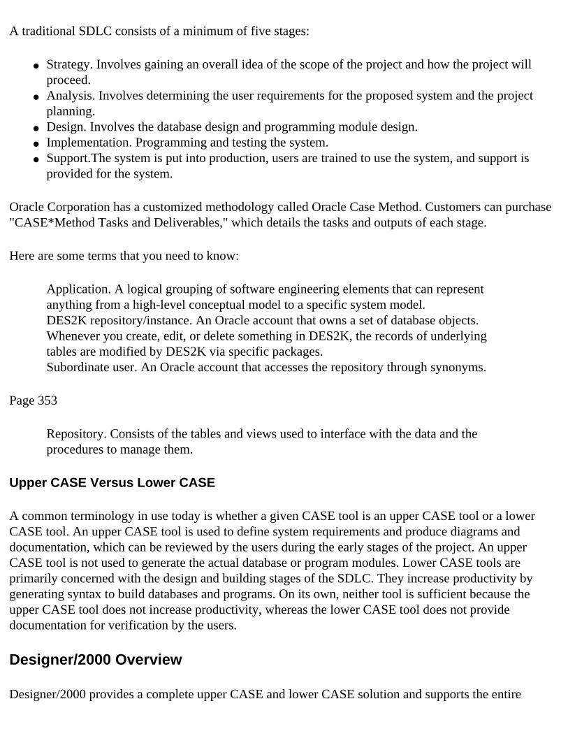
A traditional SDLC consists of a minimum of five stages:
● Strategy. Involves gaining an overall idea of the scope of the project and how the project will proceed.
● Analysis. Involves determining the user requirements for the proposed system and the project planning.
● Design. Involves the database design and programming module design. ● Implementation. Programming and testing the system. ● Support.The system is put into production, users are trained to use the system, and support is
provided for the system.
Oracle Corporation has a customized methodology called Oracle Case Method. Customers can purchase "CASE*Method Tasks and Deliverables," which details the tasks and outputs of each stage.
Here are some terms that you need to know:
Application. A logical grouping of software engineering elements that can represent anything from a high-level conceptual model to a specific system model. DES2K repository/instance. An Oracle account that owns a set of database objects. Whenever you create, edit, or delete something in DES2K, the records of underlying tables are modified by DES2K via specific packages. Subordinate user. An Oracle account that accesses the repository through synonyms.
Page 353
Repository. Consists of the tables and views used to interface with the data and the procedures to manage them.
Upper CASE Versus Lower CASE
A common terminology in use today is whether a given CASE tool is an upper CASE tool or a lower CASE tool. An upper CASE tool is used to define system requirements and produce diagrams and documentation, which can be reviewed by the users during the early stages of the project. An upper CASE tool is not used to generate the actual database or program modules. Lower CASE tools are primarily concerned with the design and building stages of the SDLC. They increase productivity by generating syntax to build databases and programs. On its own, neither tool is sufficient because the upper CASE tool does not increase productivity, whereas the lower CASE tool does not provide documentation for verification by the users.
Designer/2000 Overview
Designer/2000 provides a complete upper CASE and lower CASE solution and supports the entire

SDLC.
The logical model created during the analysis stage becomes the basis of the physical model, which is created during the design stage. Applications are generated using this model and therefore any business change is immediately reflected in the application. It also supports methodology from customers, which is not necessarily Oracle CASE method.
The minimal requirements for installing Designer/2000 are listed as follows (client side, then server side).
Client-side requirements:
● IBM, COMPAQ, or at least compatible with a 486 25DX2 processor or better. ● CD-ROM drive. ● 300MB free disk space. ● 40MB minimum swap space to run the applications. ● 16MB available memory. ● MS Windows v3.1 or higher (enhanced mode). ● MS DOS v5.0 or higher. ● SQL*NET v1.1 or v2.0 (SQL*NET is required only if running against a remote server).
Server-side requirements:
● Oracle7 v7.1.3 or higher with procedural option installed. Oracle distributed option is required if remote database reverse engineering is required. Oracle 7.3.x version or higher of Designer/2000 R 2.0.
● Shared pool size of 18MB minimum. ● Recommended optimizer mode.
Page 354
● RULE-based for R 1.3.2. ● COST-based for R 2.0. ● 40MB. ● 60MB in the SYSTEM tablespace for the repository PL/SQL packages, procedures, and views.
NOTE
Refer to the installation manuals to determine storage requirements.

For the latest information on product availability, please contact Oracle WorldWide Customer Support. As of the date of this writing, the information available is as follows (by version):
Designer/2000 R 1.3.2:
❍ Available now on both 16-bit and 32-bit platforms. ❍ Availability in Japan may be different. ❍ 32-bit is certified with Developer/2000 R 1.3.2, R 1.4, and R 1.5.1 (patches required). ❍ Contact Oracle WorldWide Customer support for required patches.
Designer/2000 R 2.0:
❍ 32-bit only.
Now let's cover information on the Designer/2000 components.
Designer/2000 Components
The Designer/2000 toolset components contain the following items:
Repository Services includes:
❍ Repository Object Navigator (RON) ❍ Matrix Diagrammer ❍ Repository Management facilities ❍ Process Modeler
Systems Modeler includes:
❍ Entity Relationship Diagrammer ❍ Function Hierarchy Diagrammer ❍ DataFlow Diagrammer
Systems Designer includes:
❍ Module Structure Diagrammer ❍ Preferences Navigator
Previous | Table of Contents | Next

Previous | Table of Contents | Next
Page 348
FIG. 14.2Conventional and direct path load methods.
Using Conventional Path Load
The conventional path uses SQL INSERT statements and in-memory bond array buffers to load data into Oracle tables. This process competes with all other processes for memory resources within the SGA. This can slow down loader performance if the database already has the overhead of supporting many concurrent processes.
Another overhead of using conventional path is that the loader process must scan the database for partially filled blocks of the table being loaded and attempt to fill those blocks. This is efficient for daily transactional processing, but it is an additional overhead that conventional path loading has.
Page 349
There are cases when conventional path is the preferred and sometimes mandatory method over the direct path:
● If the table being loaded is indexed and being accessed concurrently with the load, or inserts and deletes are being run against the table, conventional path must be used.
● When applying SQL functions in the control file, SQL functions are not allowed using the direct path.
● When the table being loaded is a clustered table. ● When loading a small number of rows into a large indexed table and/or the table has referential
integrity or check constraints. It is explained in the direct path section why conventional path is

preferred in this instance. ● When loading is done through SQL*Net or Net8 with heterogeneous platform, both nodes must
belong to the same family of computers and both must be using the same character set in order to use direct path.
Using Direct Path Load
Instead of using SQL INSERT statements and bind array buffers, direct path formats the input data into Oracle data blocks and writes them directly into the database. It is important to note that direct path loading always inserts data above the table's high-water mark. This eliminates the time spent scanning for partially filled blocks. If direct path is being used and does not complete, and loader is restarted from the beginning, the data that is loaded should be truncated or the table dropped and re-created. Simply deleting the data does not reset the high-water mark, and you will be using more storage than is necessary.
An understanding of what happens to a table's indexes using the direct path method is important to maximize the efficiency of direct path loading. In Oracle8, indexes are marked unusable when the loaded data becomes visible (the high-water mark is moved and committed), as this is the point that the indexes are out-of-date with respect to the data that it indexes. As each index is brought up-to-date, the index unusable state is cleared. This allows queries to take place against the table while direct path loading is in progress. However, a query executing while the load is in the finishing stage (moving the high-water mark and updating indexes) may fail if the query requires an index that is in an unusable state.
During the load, the new index values are written to temporary segments, and at the end of the load they are sorted and merged with the old index values, at which time the index becomes usable again. This can significantly increase the need for temp space. In order to avoid the additional need for temp space to do the sort, you can presort the data in the order of the index and use the keywords SORTED INDEXES in the control file.
In the previous section on conventional path loading, the restrictions that would prevent the use of direct path were listed. Loading a relatively small number of rows into a large table with indexes and/or referential and check constraints is not a restriction against using direct path, but it will probably be more efficient to use conventional path. In the case of the indexes, it would probably be quicker for conventional path to update the indexes as it is loading the data, rather than doing a large sort/merge to create the new indexes. With referential and check
Page 350
constraints, direct path requires that these constraints be disabled before the load. After all the data is loading and constraints are re-enabled, the entire data's table is checked against these constraints, not only the data that was loaded.

Using SQL*Loader Performance Tips
Below are some additional tips on increasing the performance of SQL*Loader:
1. Use positional fields over delimited fields, which require Loader to scan the data to search for the delimiters. Positional fields are quicker because Loader only has to do simple pointer arithmetic.
2. Specify maximum lengths for terminated by fields to make each bind array insert more efficient. 3. Pre-allocate enough storage. As data is being loaded and more space is required in the table,
Oracle allocates more extents to hold the data. This operation can be expensive if it is being done constantly during the load. Calculating or estimating the storage requirements prior to the load enables you to create the necessary storage up front.
4. Avoid using NULLIF and DEFAULTIF clauses in the control file if possible. Each clause causes the column to be evaluated for every row being loaded.
5. Split data files and run concurrent conventional path loads. 6. Reduce the number of commits by using the command-line parameter ROWS. 7. Avoid unnecessary character set conversions. Ensure that the client's NLS_LANG environment is
the same as the server's. 8. Use direct path whenever possible. 9. When using direct path, presort data for the largest index of the table and use the SORTED
INDEXES clause. 10. When using direct path, use the parallel direct path option when possible. 11. Minimize the use of redo logs during direct path loads. There are three ways of doing this with
different levels of control:Disable archiving of the database.Use the keyword UNRECOVERABLE in the control file.Alter the table and/or index with the NOLOG attribute.
Previous | Table of Contents | Next

Previous | Table of Contents | Next
Page 345
Record 3 is discarded and placed into the discard file because the flag is neither "C" nor "D," thus not satisfying either condition. Record 15 is rejected because the dollar amount is not numeric. These two records show the two stages of checking previously mentioned. Record 3 is discarded by the loader process while record 15 was not rejected until the database tried to insert it into the table.
Example 5—Loading into a Table Partition
This example (see Listings 14.15 and 14.16) is a variation of Example 4, in which we load the data from the xact.dat file. In this example, we load the data into the partition_xact table, which has four partitions to store the data by calendar quarter. A single partition or all partitions of a table can be loaded in the same loader session. In this instance, we only load partition P1 for the first quarter.
Listing 14.15LOAD5.CTL—Example 5 Control File
LOAD DATAINFILE `xact.dat'INTO TABLE partition_xact PARTITION (P1)WHEN xact_flag = `D' (acct_nbr POSITION(01:10) INTEGER EXTERNAL, xact_amt POSITION(11:20) INTEGER EXTERNAL ":xact_amt * -1", xact_flag POSITION(21:21) CHAR, xact_date POSITION(22:31) DATE "DD-MON-YY" NULLIF xact_date=BLANKS)
INTO TABLE partition_xact PARTITION (P1)WHEN xact_flag = `C' (acct_nbr POSITION(01:10) INTEGER EXTERNAL, xact_amt POSITION(11:20) INTEGER EXTERNAL, xact_flag POSITION(21:21) CHAR, xact_date POSITION(22:31) DATE "DD-MON-YY" NULLIF xact_date=BLANKS)
Invoking SQL*Loader for Example 5 from the command prompt:
$ sqlldr example/expass control=load5.ctl log=load5.log bad=load5.bad discard=load5.dis
The following is the server response:
SQL*Loader: Release 8.0.3.0.0 - Production on Fri Nov 21 14:50:32 1997
(c) Copyright 1997 Oracle Corporation. All rights reserved.
Commit point reached - logical record count 16
Listing 14.16Example 5 Log File Contents
SQL*Loader: Release 8.0.3.0.0 - Production on Fri Nov 21 14:50:32 1997
(c) Copyright 1997 Oracle Corporation. All rights reserved.
continues
Page 346
Listing 14.16Continued

Control File: load5.ctlData File: xact.dat Bad File: load5.bad Discard File: load5.dis (Allow all discards)
Number to load: ALLNumber to skip: 0Errors allowed: 50Bind array: 64 rows, maximum of 65536 bytesContinuation: none specifiedPath used: Conventional
Table PARTITION_XACT, partition P1, loaded when XACT_FLAG = 0X44(character `D')Insert option in effect for this partition: INSERT
Column Name Position Len Term Encl Datatype------------------------------ ---------- ---- ---- ---- --------------ACCT_NBR 1:10 10 CHARACTERXACT_AMT 11:20 10 CHARACTERXACT_FLAG 21:21 1 CHARACTERXACT_DATE 22:31 10 DATE DD-MON-YY
Column XACT_AMT had SQL string":xact_amt * -1" applied to it.Column XACT_DATE is NULL if XACT_DATE = BLANKS
Table PARTITION_XACT, partition P1, loaded when XACT_FLAG = 0X43(character `C')Insert option in effect for this partition: INSERT
Column Name Position Len Term Encl Datatype------------------------------ ---------- ---- ---- ---- --------------ACCT_NBR 1:10 10 CHARACTERXACT_AMT 11:20 10 CHARACTERXACT_FLAG 21:21 1 CHARACTERXACT_DATE 22:31 10 DATE DD-MON-YY
Column XACT_DATE is NULL if XACT_DATE = BLANKS
Record 3: Discarded - failed all WHEN clauses.Record 5: Rejected - Error on table PARTITION_XACT, partition P1.ORA-14401: inserted partition key is outside specified partitionRecord 10: Rejected - Error on table PARTITION_XACT, partition P1.ORA-14401: inserted partition key is outside specified partitionRecord 14: Rejected - Error on table PARTITION_XACT, partition P1.ORA-14401: inserted partition key is outside specified partitionRecord 15: Rejected - Error on table PARTITION_XACT, column XACT_AMT.ORA-01722: invalid numberRecord 16: Rejected - Error on table PARTITION_XACT, partition P1.ORA-14401: inserted partition key is outside specified partitionRecord 4: Rejected - Error on table PARTITION_XACT, partition P1.
Page 347
ORA-14401: inserted partition key is outside specified partitionRecord 6: Rejected - Error on table PARTITION_XACT, partition P1.ORA-14401: inserted partition key is outside specified partitionRecord 8: Rejected - Error on table PARTITION_XACT, partition P1.

ORA-14401: inserted partition key is outside specified partitionRecord 12: Rejected - Error on table PARTITION_XACT, partition P1.ORA-14401: inserted partition key is outside specified partitionRecord 13: Rejected - Error on table PARTITION_XACT, partition P1.ORA-14401: inserted partition key is outside specified partition
Table PARTITION_XACT, partition P1: 3 Rows successfully loaded. 5 Rows not loaded due to data errors. 8 Rows not loaded because all WHEN clauses were failed. 0 Rows not loaded because all fields were null.Table PARTITION_XACT, partition P1: 2 Rows successfully loaded. 5 Rows not loaded due to data errors. 9 Rows not loaded because all WHEN clauses were failed. 0 Rows not loaded because all fields were null.Space allocated for bind array: 7168 bytes(64 rows)Space allocated for memory besides bind array: 0 bytes
Total logical records skipped: 0Total logical records read: 16Total logical records rejected: 10Total logical records discarded: 1
Run began on Fri Nov 21 14:50:32 1997Run ended on Fri Nov 21 14:50:33 1997
Elapsed time was: 00:00:00.31CPU time was: 00:00:00.04
Example 5 comments: To load a partition of a partitioned table, the keyword PARTITION needs to be added after the table name in the control file. Note that the partition name, in this instance P1, must be enclosed in parentheses. All partitions are loaded if the keyword PARTITION is omitted. All records that are not in P1's partition range are written to the bad file.
Conventional and Direct Path Loading
SQL*Loader provides two methods to load data, conventional and direct path loading. Conventional path loading is the default for SQL*Loader. To enable direct path loading, DIRECT=TRUE must be added to the command-line parameters when invoking SQL*Loader. As seen in Figure 14.2, conventional path loading has additional steps that direct path loading doesn't. These extra steps add overhead to the process, making conventional path slower than direct path. The additional steps of formatting SQL INSERT statements and going through the buffer cache of the SGA are contending with all other processes that are running concurrently against the database. Although the inclination is to always use direct path for its speed, there are restrictions and cases in which conventional path should be used. This is covered in the following section.
Previous | Table of Contents | Next

Previous | Table of Contents | Next
Page 355
● Module Logic Navigator ● Data Diagrammer ● Module Data Diagrammer ● Generators
The Designer/2000 components are shown in Figure 15.1.
FIG. 15.1The Designer/2000components.
Understanding the Repository
The heart of Designer/2000 is the repository that records all the information entered into Designer/2000. It is the basis for generation in the build stage of the SDLC. Features include:
● Repository Object Navigator (RON). A part of the repository services that allows a highly intuitive method of viewing and manipulating repository objects.
● Repository-based. This allows multiuser concurrent access, check-in and check-out facilities available, and data access from other products such as SQL*PLUS.
● Version control. This allows the development to proceed with the current state of the application frozen. It allows the maintaining of a history of system development over time and also parallel development of the application using one or more versions. For example, an inventory system can be developed for use in both the United States and the UK—one version containing UK-specific details, and the other containing U.S.-specific information.
● Quality checks. It provides a variety of quality checks during the initial stages by cross-referencing and checking consistency rules that allow the fixing of errors during the early stages.
● Documentation. It offers an extensive set of reporting options to generate systems documentation. All the information is entered into property sheets and diagrammers

Page 356
as the project progresses; the reports are available easily. There are over 100 standard reports that can be run.
● National Language support. It allows Designer/2000 to be run against an Oracle database built in any character set, including multibyte character sets.
Several reports can be obtained from the repository, as shown in Figure 15.2.
FIG. 15.2The reports availablefrom the repository.
Using the Diagrammers
Features common to all diagrammers of the Designer/2000 toolset are as follows:
● Graphical user interface ● Point and click ● Pull-down menus ● Context-sensitive help ● Multiple windows ● Integration with the repository ● OLE 2.0 integration ● Hierarchical views
All diagrammers and utilities provided with DES2K have certain common aspects, and you can use similar steps to interface with them. After Designer/2000 has been installed, you will see an Oracle Designer/2000 icon in the Designer/2000 group. Double-click this icon and log on
Page 357
to the Oracle database where the repository resides. If you are opening an existing application system, choose it at this point. Otherwise, you can create a new application system at this point.

NOTE
The Designer/2000 window can be started from the command line using the following syntax:DES2KXX username/password@database /A:apps_system,version /S where username/password@database is the connect string; /A specifies the application system and the version; and /S is used to suppress the splash screen.
To create a new application system, complete the following steps:
1. Select RON and choose File, New. 2. Create a name for the application system.
You can continue working with this application system or change it by choosing a different one from the File menu.
The main DES2K window has buttons to start all diagrammers and utilities as well as context-sensitive links to the help system. The status line of the different tools and utilities contains valuable information about the current session, such as the application system, version, and logged-on user. All the diagrammers have a similar look and feel. They have a Multiple Document Interface (MDI) and enable the user to look at the same object from different views and through different diagrams at the same time.
The diagrammers make extensive use of the mouse to manipulate objects and also respond to dialog boxes. All the standard Windows mouse actions such as drag-and-drop, selecting, double-clicking to change the properties, moving, resizing, and so on are supported. A full-featured menu system allows easy manipulation of the objects and the application systems. A toolbar is also provided as an extension of the menu system and makes the most frequently used functions easily accessible to the developers. The DES2K utilities also have a common look and feel. Two types of utilities are used:
● Full-window utilities such as Repository Object Navigator, Repository Administration, Repository Reports, Preferences Navigator, and Matrix Diagrammer provide an MDI interface similar to the diagrammers. These utilities provide an object navigator and properties window to easily manipulate the objects.
● Pop-up window utilities such as the generators and reverse engineering utilities are generally started from another diagrammer or utility.
Diagramming Techniques Used by Designer/2000
During the logical and physical design of a system, diagrams help us accurately document the proposed system and communicate with the users and other team members. The following Designer/2000 diagrammers are commonly used during the logical and physical design of the database:

Page 358
● Entity relationship diagrammer. An ERD models the information needs of an organization. It should involve communication and consensus between the project team and the end users. Entity relationship modeling involves identifying the things of importance in an organization (entities), the properties of those things (attributes), and how they relate to each other (relationships). A simple two-entity ERD is shown in Figure 15.3.
FIG. 15.3An example of a two-entity relationshipdiagram.
● Function hierarchy diagram. This identifies everything the company needs to do and shows functions that the company performs and those that it wants to implement in the future. The function hierarchy begins with an overall mission description and breaks it down into major functions that are further decomposed until it is not possible to break it further.
● Dataflow diagram. The DFD depicts how information flows in the business and how it flows between the outside environment and the system interfaces.
● Matrix diagrams. The repository services of Designer/2000 allow the generation of a variety of matrix diagrams for the system. The purpose of the matrix is to identify areas that might have been overlooked during the logical design stage.
● Process flow diagram. The process modeler component of Designer/2000 supports process modeling techniques that can be used to support Business Process Re-
● engineering (BPR) or prototyping. It can also act as a means of visual feedback to the users about the analyst's understanding of the system requirements.
● Data schema diagrams. Graphical representations of the interrelated tables and constraints in the database. Primary and foreign keys are shown in the diagram, which
Previous | Table of Contents | Next

Previous | Table of Contents | Next
Page 359
might also show the views, snapshots, and columns of the tables. The DSD is created during the design stage and uses the ERD from the analysis stage. Figure 15.4 shows a schema obtained from this diagrammer.
FIG. 15.4An example of aschema.
● Module data design. Depicts one program module. Typically, a system will have several module data diagrams—one for each screen, report, and batch utility. It is usually based on the Function hierarchy diagram and feeds information directly to the forms and reports generators.
● Module structure diagram. Shows the interrelationship of the modules defined by the module data diagrammer. It is created during the design stage.
Generators
Several code generators are provided by Designer/2000, and these are repository utilities that allow the generation of complete, bug-free code to be used in the build phase of the System Development Life Cycle. The collection of generators can be classified into two types: Server Code Generator and Front-End Code Generator.
Forms GeneratorThis DES2K component allows Developer/2000 applications to be built quickly based on repository information. Forms generator has a lot of features, including
● Generating full-featured and menued forms applications ● Integrating with the systems designer
Page 360
● Enabling generation of applications with GUI items such as buttons, check boxes, radio groups,

and so on ● Providing foreign-key validation ● Providing implementation of business rules ● Reverse engineering of Oracle forms applications and storing it in the repository ● Regeneration of forms without losing code enhancements added by developers ● Support for VBX controls for 16-bit versions and OCX controls for 32-bit versions ● OLE 2.0 support and integration with Windows-based desktop applications
Figure 15.5 shows the forms generator in use.
FIG. 15.5An example of the formsgenerator in use.
Reports GeneratorThe reports generator is a DES2K component that enables Oracle reports applications to be built quickly, based on repository information. Its many features include:
● Supports multilink reports ● Provides many reporting styles and layouts including control break, master-detail, and matrix
reports ● Provides productivity gains to developers ● Provides templates for standardization ● Customization of generator operations ● A variety of summary functions ● Reverse-engineering from existing reports and creates module definitions stored in the repository ● Regeneration of reports with changed specifications
Page 361
Server GeneratorThis Designer/2000 component allows for the creation of database objects and PL/SQL modules based on repository information. Its features include:
● Generates ANSI standard SQL for database object creation ● Generates check constraints

● Generates and validates PK-FK relationships ● Supports the role-based security of Oracle7 ● Generates PL/SQL modules including triggers, procedures, functions, and packages ● Snapshots ● Reverse-engineers database objects and stores their definitions in the repository
Basically, you define the objects in the repository and then use this generator to specify the object for which you want the script created.
Figure 15.6 shows the server generator used to generate DDL.
FIG. 15.6An example of the useof the server generator.
Visual Basic GeneratorThis generator is similar to the forms generator. The code from this generator can be loaded into Visual Basic 4.0 and is used to create an executable file.
Figure 15.7 shows a Visual Basic generator.
WebServer GeneratorThe WebServer Generator can be used to create Web applications. To create a Web application:
1. Define the modules in the module data diagrammer. 2. Create PL/SQL packages from the modules using WebServer. 3. Run the generated PL/SQL scripts on Oracle WebServer to create the Web application.
Page 362
FIG. 15.7An example of a VisualBasic generator.

MS Help GeneratorThe MS Help Generator creates help files in MS Help file format that can be used with forms and Visual Basic applications. The MS Help Generator puts help text in a file and creates the necessary links and jumps. You will also need the MS Help Compiler, a separate product, to generate the WinHelp format files.
C++ Object Layer GeneratorThis generator allows you to access object-relational databases by creating C++ class definitions and code using the systems modeler tools. It can be used to produce the classes for both the data and the functions that form the object. You will need to compile the generated classes with the rest of the C++ code and also link it with the C++ libraries.
Module Regeneration Strategy
All the post-generation work should be implemented in such a way that module regeneration can take place more or less in a painless manner. The following strategies can be used to accomplish this task:
● Put all the information in the repository. This method ensures that the changes are automatically applied in the regenerated modules. However, this method results in increased administration of the repository.
● Use multiple templates—a base template and other form-specific templates. The base template can be used for all the forms in the system. You can also put form-specific information in the other templates, thereby making it easy to manage the code.
Oracle CASE Exchange
Oracle CASE Exchange is a utility that allows bidirectional exchange of information between Designer/2000 and CASE tools from other vendors. This can be very useful for people who have been using CASE tools from other vendors and are now interested in using Designer/2000. It is especially useful if an organization does its analysis using another CASE tool like
Page 363
LBMS Automate Plus and now wants to finish the project using Designer/2000. One limitation of DES2K is that it does not generate 3GL code; by using CASE exchange, one can transfer the information from the repository into another CASE tool and generate 3GL from that tool.

Oracle CASE exchange supports the CASE tools described in the following lists.
Upper CASE support includes:
● ADW/IEW from Knowledgeware ● Excelerator from Intersolv ● Design/1 from Anderson Consulting ● LBMS Automate Plus
Lower CASE support includes:
● ASK Ingres 6.0 ● Pansophic Telon
Validation checks are provided by CASE exchange for the following before loading:
● Entities without attributes ● Attributes without an entity ● Entities without relationships ● Entities without unique identifiers ● Compatibility with the target tool
Waterfall-Oriented Methodology Using Designer/2000
The following are the steps involved in CASE studies: Strategy, Analysis, Design, and Implementation:
1. Create an application, which will be your work area. Use Repository Object Navigator (choose File, New).
2. By using the entity relationship diagrammer, create the entities and their relationships. Use Edit, Domain to enter domains, their valid values, and their defaults. Double-click an entity to enter attributes, and to specify its domain and relationships. Also add attribute defaults and valid values.
3. Use the function hierarchy diagrammer to create this diagram. Double-click each function and add additional information to determine whether it will be a module or a form.
4. By using the matrix diagrammer, specify the correlation between functions and entity attributes. 5. Use the various reports to examine the quality of your analysis. 6. Use the properties window to define an area where the database objects will reside.
Previous | Table of Contents | Next

Previous | Table of Contents | Next
Page 393
CHAPTER 16
Oracle Web Application Server 3.0
In this chapter
● Introducing the Oracle Web Application Server 394 ● Understanding the Network Computing Architecture (NCA) 394 ● Understanding the Oracle Web Application Server 395 ● Providing Basic Services with the Oracle Web Application Server 398
Page 394
Introducing the Oracle Web Application Server
The Internet burst into the consciousness of most people within the past 18 to 24 months. The Internet was seized upon by the media and by computer users as something new, unlike any computing innovation that preceded it.
The Internet has also added some new standards to the computing environment. With the nearly universal addressing scheme offered by the Internet and TCP/IP, the standard mail and other protocols offered by the Internet services, and an easy, cross-platform hypertext display standard in HTML, the Internet provides a way to integrate dissimilar computers across the world.
Oracle has been a leader in providing database technology for the past 15 years, and because the Internet is a gigantic network for exchanging data, it makes sense that Oracle products should play a role in the retrieval and dissemination of data over the Internet and through Internet-based applications.
The Oracle Web Application Server is the basis for Oracle's use of the Internet. However, it is also much more than just a way to use the Internet. The Oracle Web Application Server is a key piece of the Network Computing Architecture (NCA), which is, in turn, the blueprint for the implementation of a completely distributed application system. Internet-based applications are a type of distributed application, so the Oracle Web Application Server is ideally suited for Web-based applications as well. The rest of this chapter introduces you, at a high level, to the Oracle Web Application Server. The rest of this book will help you create systems that are implemented over the Internet or an intranet and use the services of the Oracle Web Application Server.

Understanding the Network Computing Architecture (NCA)
The Network Computing Architecture is a framework that can be used to create open, distributed application systems. To understand the NCA, it helps to take a look at the evolution of the computing infrastructure over the past few years.
Ten years ago, virtually all applications were deployed on a single monolithic machine, with users connected to the machine by dumb terminals. Different software components running on the machine were used to implement systems, such as database management systems and application programs, but all the components communicated with each other through shared resources, such as disk and memory, or, at worst, over an internal communication bus.
As personal computers (PCs) began to enter the computing landscape, the client/server model began to be used for application systems. Client/server computing featured personal computers as clients, with enough power to support the graphical user interfaces demanded by users, as well as the execution of application logic, connected over a local area network to a database server. It took several years for developers and the tools that they used to appropriately
Page 395
support the client/server architecture and reduce the impact of the bottlenecks imposed by limited network bandwidth.
The client/server computing architecture was widely favored by users, but the distribution of computing resources over a wide number of client machines created its own set of problems for application developers and system administrators. Whenever applications changed, new client components had to be distributed to all client machines, and the growing complexity of application logic began to strain the limits of the computing power on PC clients. To address both of these issues, a three-tier computing model evolved, where application logic was run on a server machine that acted as an intermediary between the client and the database server.
The NCA has been introduced to extend the three-tier model into a multitier model. The NCA provides a standard interface that can be used by a variety of cartridges, which are self- contained units of functionality that can act as client components, application logic components, or data components. The Network Computing Architecture also includes a standardized communication protocol, so that the different cartridges in an NCA application can communicate with each other. The basic structure of the Network Computing Architecture is illustrated in Figure 16.1.
FIG. 16.1The Network Computing

Architecture provides a framework fordistributed computing.
The NCA is also ideally suited for Internet applications. A Web client, in the form of a browser, can use the NCA framework to interact with other application components. The same components can be used as cartridges within a more traditional client/server architecture, or even with dumb terminals connected to a monolithic computer. By clearly defining the ways that client, logic, and data cartridges interact, the NCA allows virtually unlimited flexibility in creating and deploying application systems.
Understanding the Oracle Web Application Server
The Oracle Web Application Server plays a key role in the Network Computing Architecture and acts as the focal point for the management of cartridge services and the communication between cartridges.
Page 396
The illustration of the Network Computing Architecture presents a conceptual view of the NCA. The Oracle Web Application Server provides some of the substance that is needed to make the Network Computing Architecture a reality.
A cartridge is a code module which interacts with the Oracle Web Application Server through a standard interface. The basic function of the Oracle Web Application Server in the NCA is to manage the interaction of cartridges. To accomplish this, the Oracle Web Application Server manages the creation of application logic cartridges, the communication between client cartridges and application logic cartridges, and the inter-cartridge communication between application logic cartridges. The Oracle Web Application Server also provides basic services to cartridges that are necessary to implement robust applications using the Network Computing Architecture.
The Oracle Web Application Server is composed of the following three basic components:
● The Web Listener, which handles communication between clients and the Web Application Server through standard Internet protocols.
● The Web Request Broker, which manages the creation of cartridge processes; load balancing between multiple instances of individual cartridges; and services to cartridges, such as transaction services, inter-cartridge communication services, persistent storage services, and authentication services.

● Specific cartridges which are used to implement specific application functionality.
This layered architecture gives Oracle Web Application Server two basic advantages. First of all, it allows each component to be designed to best address the needs of its particular function, instead of trying to handle all of the tasks of a server. For instance, the Web Listener must be ready to receive all HTTP messages, so it should be a small application to be as responsive as possible. Web Request Broker, on the other hand, will potentially have to handle many different types of requests, so it will have to be able to manage multiple tasks, requiring a more robust application.
The Oracle Web Application Server can support multiple instances of individual cartridges, which makes applications that use these cartridges highly scalable. This scalability is enhanced by the ability to add additional resources where you need them, without affecting the rest of the components. For instance, you can have multiple listeners to handle high volume traffic, or spawn additional cartridge instances if a particular cartridge's functionality is heavily taxed.
The second advantage comes from having a well-defined application program interface between the different components. This interface makes Oracle Web Application Server an open system, to which you can add your own custom components to create your system. For instance, you can substitute some other HTTP listener for Oracle Web Listener and still use the other components of the Oracle Web Application Server. Even more importantly, the open architecture of Oracle Web Request Broker allows you to write your own cartridges, to support any development environment, and to deliver any type of functionality you need in your Web applications.
Previous | Table of Contents | Next

Previous | Table of Contents | Next
Page 389
Table 15.10 details the Designer/2000 supported-versions list (please contact Oracle WorldWide Support for an updated list for Designer/2000 R 2.0).
Table 15.10Designer/2000 Supported Versions
Designer/2000 Release 1.32 (16-bit)
Release 1.32 (32-bit)
Platform Windows 3.1, NT 3.5.1, and OS/2 3.0 Warp
Win95, NT 3.5.1, and NT 4.0
Version Number 6.0.10.0.1 6.0.10.0.0
Server Version 7.3.2.1 and 7.3.2.3 7.3.x and 8.0.3
Forms 4.5.7.1.2E 4.5.7.1.6
Reports 2.5.5.2.5C 2.5.5.2.5C
Graphics 2.5.7.1.0D 2.5.7.1.0C
Procedure Builder 1.5.6.14.0 1.5.6.15.3
Discovery Browser 2.0.9.2.7 2.0.9.2.8
SQL*PLUS 3.3.2.0.2 3.3.2.0.2
SQL*NETV1 ————— —————
SQL*NETV2 2.3.2.1.6 2.3.2.1.6A
Oracle Installer 3.1.4.1.2F 3.1.4.1.3
Forms Generator 4.5.10.0.1 4.5.10.0.0
Reports Generator 2.5.10.0.1 2.5.10.0.0
Server Generator 1.0.10.0.1 5.5.10.0.0
Visual Basic Generator
1.0.10.0.1 1.0.10.0.0
Visual Basic Professional Edition V4 (16-bit)
Professional Edition V4 (16-bit)
Oracle Objects for OLE
V2 V2

C++ Object Layer Generator
1.0.10.0.0 1.0.10.0.0
Visual C++ MS Visual C++ 1.52, 2.2, 4.1
MS Visual C++ 1.52, 2.2, 4.1
Web Generator 1.0.10.0.1 1.0.10.0.0
Oracle Web Server Option
V2 V2
MS Help Generator 1.0.10.0.1 1.0.10.0.0
Page 390
Table 15.11 describes the Designer/2000 utility and the corresponding executable filename.
Table 15.11Mapping of Tools to the Executable
Designer/2000 Utility Executable Filename
Data Diagrammer dws13.exe
Dataflow Diagrammer awd23.exe
Designer/2000 Diagnostics ckndiag.exe
Entity Relationship Diagrammer awe23.exe
Forms Generator cf45g32.exe
Function Hierarchy Diagrammer afw23.exe
Graphics Generator cg25g32.exe
Matrix Diagrammer awm23.exe
Module Data Diagrammer iwmdd13.exe
Module Logic Navigator iwmln13.exe
Module Structure Diagrammer dwm13.exe
MS Help Generator cvhpg13.exe
Preferences Navigator iwgpn13.exe
Process Modeler bpmod13.exe
Reports Generator cg25r32.exe
Repository Administration Utility ckrau13.exe
Repository Object Navigator ckron13.exe
Repository Reports ckrpt13.exe
RON Load Utility ckld13.exe
VB Generator cvvbg13.exe

WebServer Generator cvwsg13.exe
Page 391
PART IV
Oracle on the Web
16. Oracle Web Application Server 3.0 17. Web Application Server Components 18. Installing and Configuring the Oracle Web 19. Application Server
Page 392
Previous | Table of Contents | Next

Previous | Table of Contents | Next
Page 386
querying tables. However, keep in mind that views are just stored select statements and can be used post-generation for the minor changes requested by the users, such as new reports or security changes to the application.
● Before the creation of modules, make sure that the default data is entered. Before modules are created, default data should be entered in the table definitions. The following defaults can be verified for every table: display datatype, display sequence, format, prompt, hint, default order sequence, and display length and width. This will save a lot of time when modules needed to be redeveloped.
● Display meaningful error messages. When users enter invalid information in fields, it is better to provide meaningful error messages to them that indicate what the valid values are rather than give them meaningless system-generated errors.
● Enforce standards. Standardization in development can lead to increased development efficiency, reduction of maintenance, and reduction in the learning curve for new developers. Designer/2000 provides many reports that enforce standards. It also provides an API that consists of a set of views against the repository tables and a set of PL/SQL packages that enable the repository to be updated. The API can be used to generate reports that list/fix the violations in the standard.
● Learn about the generation preferences of forms and reports. The time spent in understanding the preferences during generation pays off at the end by reducing post-generation efforts.
● Set the default preferences for the application. Become familiar with the preferences that can be set at the application level and should be left unchanged for the generated modules. Other preferences can be used for each generated module as needed to conform to the design standards.
● Learn and use the forms and reports generators. Many developers like to use the Designer/2000 generators to generate a skeleton form or report and do most of their development using Developer/2000. However, the DES2K generators are quite useful, and if you take the time to understand their capabilities, it will result in a high percentage of generation.
● Involve users to a certain extent in the project. It definitely helps to get user approval for the prototype, and constant communication with the users is essential. But after a certain point the users should not be allowed to make suggestions; otherwise, the system will be constantly changing, and user expectations can become very high.
● Post-generation should start after all the modules are generated. If post-generation is started at an early stage, major changes in data design will be difficult to incorporate in the final modules.
● Document post-generation steps. Use the DES2K repository to store a detailed description of post-generation steps so that the developers can easily reapply these steps if there is (and usually there is) a need to reapply the steps. You can use the module's text fields like "notes" or create your own custom text fields to store this information.
● Customize the templates. DES2K provides a number of templates that can be customized to

implement specific needs.
Page 387
● PL/SQL should be placed in library functions, procedures, and packages. This will simplify code maintenance of the modules. The template code can access these libraries, and if there is any change to the code in the library, the modules will immediately reflect the changes without recompilation.
Designer/2000 R 2.0 Features
Designer/2000 Release 2.0 provides a variety of new features. These features include:
Extended Server Generation:
● Support for Oracle7, Oracle RdB, Oracle Web Server ● Support for non-Oracle databases: MS SQL Server, Sybase, DB2/2, and Informix ● Support for ODBC databases ● API generation for DML and lock procedures for tables
Client Generation:
● Design Reuse: Once a module is defined, its components can be shared with other modules. ● Application logic: Store PL/SQL, Visual Basic and Java code. ● Generators integration. ● Generation of database triggers based on declarative design information in the repository. ● One hundred percent reverse engineering of application logic as well as one hundred percent
generation.
Design Editor:
● A single fully integrated design and generation environment. ● Maximize ease-of-use by means of wizards, drag and drop, edit-in-place, right mouse menus, and
synchronized updates.
Migration Paths to Designer/2000 R 2.0:
● Designer/2000 R 2.0 can perform upgrades on Designer/2000 R 1.x repositories. ● A separate utility will be provided for upgrading from CASE 5.0.x and 5.1.x to Designer/2000 R
1.3.2. The repository can then be brought up-to-date with R 2.0.

Application Upgrades:
● The Restore facility in the RON can be used to upgrade a pre-existing Release 1 application or a set of applications to Designer/2000 R 2.0. A two-step process upgrades the archived applications to be 1.3.2-compliant and then upgrades this to R 2.0.
● The disadvantage of this approach is that if the upgrade process is aborted due to errors, it has to be restarted with the original archive. To prevent this from happening, analyze the data before archiving it.
Page 388
Coexistence of Release 1.x and Release 2.0:
● 16-Bit Release 1.x—Yes, provided that the 16-bit Release 1.x and the 32-bit Release 2.0 are in separate Oracle homes.
● 32-Bit Release 1.x—Yes. Installing Release 2.0 on top of existing Release 1.x will not be a problem, because the default directory names are different in Release 2.0.
Cautions:
● The NLS_LANG parameter in the Registry must match the NLS_LANG parameter in the server; otherwise, it will cause problems when loading package definitions during install and upgrade.
● A typical upgrade should take 2_3 hours to drop the existing API, and another 2_3 hours to load the new API and perform instance conversion and initialization.
● If the RAU has invoked SQL*PLUS, do not manually invoke SQL*PLUS; it can lead to process hands and even corruption of the repository.
Designer/2000 and Oracle8
The introduction of Oracle8 has taken the databases and the applications built on those databases to a whole new level, both in the amount of data stored and the number of users supported. Designer/2000 provides a complete set of modeling and generation tools for the relational and object constructs of Oracle8.
Designer/2000 2.0 provides support for all the Oracle8 scalability features, including:
● Partitioning of tables ● BLOBs (binary large objects) and CLOBs (character large objects) ● Index organized tables (IOTs) ● Deferred constraint checking ● Type tables ● Collections

● Object views (represent a relational structure as though it were a type) ● Embedded types ● VARRAYS (multivalued columns) ● Nested tables (tables embedded within other tables) ● References (directly reference one object from another)
Designer/2000's schema modeler has been extended to use the scalability and object features of Oracle8 without compromising ease of use. It allows you to design database schema or load existing schema definitions into its repository. The server generator then translates the graphical representation into the appropriate SQL DDL to implement it. Designer/2000 uses unified modeling language (UML), an emerging open standard from the Object Management Group (OMG) to represent its type models.
Previous | Table of Contents | Next

Previous | Table of Contents | Next
Page 397
The Web Listener
The Web Listener, as the name implies, listens for HTTP requests coming to the IP address of the server machine. When Web Listener gets a request, it passes the request on to Web Request Broker. Web Request Broker tries to identify the type of request by checking to see whether the directory of the request's URL can be mapped to a directory that is associated with one of the cartridges of the server. If the URL does map, the request is executed by the appropriate cartridge. If the URL does not map to one of the associated directories, the URL is passed back to Web Listener and the document represented by the URL is retrieved.
The Web Request Broker
What's under the hood of Web Request Broker? When a request comes in for a particular Web Service, a Web Dispatcher passes the request to the Web Service. The Web Dispatcher handles assigning a request for a cartridge to a particular Web Service, which is labeled as a WRBX in Figure 16.2. Each Web Service is a multithreaded process, and each service request has its own thread. This saves the overhead of starting a process for each request. You can have more than one service for a cartridge and specify the maximum and minimum number of threads for the service, so the Web Dispatcher performs dynamic load balancing between multiple services.
FIG. 16.2The architecture of the Oracle Web ApplicationServer handles theassignment of tasksto Web request engines.
Each service has its own execution engine and uses a shared library. The Web Request Broker execution engine communicates with cartridges through three basic Application Program Interface (API) calls to initialize a service, shut down the service, and pass requests to the service.
Cartridges

Oracle Web Application Server comes with the following six predefined cartridges:
● A PL/SQL cartridge, which can call PL/SQL packages ● A Java interpreter cartridge, which provides a runtime Java execution environment ● A Perl cartridge, which can call Perl scripts ● An ODBC cartridge, which provides access to a variety of data sources using the Open Database
Connection interface
Page 398
● A VRML cartridge for implementing VRML applications ● A LiveHTML cartridge to work with server-side includes
The PL/SQL and Java cartridges include additional functions that extend the capability of the cartridge to perform extended processing, such as writing HTML back to a browser.
Oracle will also be delivering a Web cartridge interface for applications developed with its Developer/2000 for the Web product in the second quarter of 1997. The Web cartridge for Developer/2000, as illustrated in Figure 16.3, will allow any application created with Developer/2000 for the Web to be re-compiled and deployed over the Web, with a Java applet acting as a user interface on the client and the application itself running on a Web server.
FIG. 16.3Developer/2000 for the Web uses a Webcartridge to imple-ment application systems.
The Web Request Broker uses an open API, so you can design your own cartridges. You can create system cartridges, which execute a predefined function, or programmable cartridges, which can be used to interpret runtime applications. Third-party developers can also develop cartridges for specific purposes. Any new cartridge can be easily integrated into the open Web Application Server environment by registering the cartridge in the Web Application Server configuration file.
Providing Basic Services with the Oracle Web Application Server
The Oracle Web Application Server provides some basic services that can be used by any cartridge. There are four basic categories of services provided by Oracle Web Application Server:

● Transaction services ● Inter-Cartridge Exchange services ● Persistent storage services ● Authentication services
In addition, the Oracle Web Application Server provides a log server to log requests to the Oracle Web Application Server and a log analyzer, which helps to understand the server logs.
Page 399
Transaction Services
The Oracle Web Application Server provides transaction services to all cartridges. A transaction is a clearly defined unit of work. If a transaction is committed, all changes implemented by the transaction are applied to the relevant data stores. If a transaction is rolled back, which means that the data is returned to the state it was in prior to the start of the transaction, the data stores are left in the same state they were in prior to the start of the transaction. By providing transaction services, the Oracle Web Application Server allows you to overcome the problems faced by the stateless nature of HTTP communication.
Inter-Cartridge Exchange Services
The Oracle Web Application Server provides Inter-Cartridge Exchange services, which allows different cartridges to communicate with each other.
In Release 3.0 of the Oracle Web Application Server, the internal communications between cartridges are handled by an internal communication protocol that is compliant with the Common Object Request Broker Architecture, also known as CORBA. The CORBA standard is an open protocol that is supported by a wide variety of hardware and software vendors.
Subsequent releases of the Oracle Web Application Server will extend the use of the CORBA standard for Inter-Cartridge Exchange so the independently developed CORBA components will be able to transparently interact with NCA cartridges through the use of the Oracle Web Application Server.
Persistent Storage Services
The Oracle Web Application Server includes a set of application programming interfaces that allow developers to read and write data objects, create data objects, and delete data objects and their data. These APIs can be used to write data to either the Oracle7 database or to native files on the server platform.

These APIs are built on a schema that includes attributes such as content type, author, and creation date. The persistent storage services allow all cartridges to operate through a common interface whenever data has to be stored on disk or for future reference within an application.
Authentication Services
Release 3.0 of the Oracle Web Application Server gives developers a variety of extensible authentication schemes that can be used in their applications including basic, digest, domain, and databased authentication.
The authentication services give developers the flexibility to implement security in the way which is best suited to the needs of their particular application.l
Previous | Table of Contents | Next

Previous | Table of Contents | Next
Page 400
Previous | Table of Contents | Next

Previous | Table of Contents | Next
Page 401
CHAPTER 17
Web Application Server Components
In this chapter :
● Examining the Web Listener 402 ● Examining the Web Request Broker 404 ● Examining the Web Application Server SDK 408
Page 402
Examining the Web Listener
Oracle Web Application Server uses Web Listener to wait for incoming requests for services. Typically, such a listener would set up an address that serves as an electronic signpost to tell all wayfaring packets of data, "I'm open for business." Of course, the listener must tell Oracle Web Application Server its address before opening for business. When Oracle Web Application Server has this address registered, it can build a road to Web Listener. This way, when a client issues a request, Oracle Web Application Server can route the message on to Web Listener, which then can execute the appropriate service.
Getting Into More Details
Web Listener processes one or many simultaneous client or remote server requests, in which case the remote server is acting as a client. For remote requests to be issued, you must make sure that the Web Request Broker object has been instantiated first. Otherwise, the remote listener won't exist and client requests can't be issued remotely.
After these communication channeling objects are in place, a client issues a request to Web Listener. Web Listener first checks to see whether this incoming message is a request for a static document or a dynamic document. If it's a static document, Web Listener returns to the client a "packet" that contains the file and the associated type information. If the client requests a dynamic document, Web Listener invokes a method (program) to create the document.
Web Listener executes its task so that it's compatible with the Common Gateway Interface (CGI). Web Listener uses CGI to invoke a method on the Web Agent object when a client requests a remote or local

database procedure. All logging activities are automatic unless you started the listener through the Listener Administration page or the Boot page. In this case, you can manually start the logging service by updating the Log Info section in Web Listener administration forms.
Finally, regarding the HTTPD listener process, Oracle has decided that root ownership of this process violates overall system security. It doesn't disappear—it just gets bumped down the listener hierarchy, replaced at the top of the hill by the admin listener. In Oracle Web Application Server 3.0, you have to start the admin listener at the root level. This particularly helps companies that have advanced workgroup models with various security levels per workgroup and per role within each workgroup. So now you create, modify, or start each listener by group, user (or by role), or as running at port 1024.
To create, modify, or start a listener, enter the following command at the prompt:
owsctl start/stop admin 2
Based on the needs of the request, your admin listener becomes a virtual DBA, in a sense, as it issues database requests that require DBA permissions. Such requests could be to create new
Page 403
users. For this implementation to work properly, you or your database administrator will need to include the admin listener owner in your Oracle database's DBA group.
Understanding Web Listener's Architecture
Although multithreaded processing is a must in today's mission-critical client/server environment, some IS technicians have overused and abused this technology. What they neglect to understand—and it's easy to do so—is that each process needs memory and resources allocated to it. Without the appropriate memory and resource allocation, system performance can slow as more threads are opened, especially where processes handle requests synchronously. Therefore, you need to put a lot of thought into implementing multithreaded architectures.
Oracle designed Web Listener with this in mind. Web Listener's only task is to accept incoming client requests and route them to the Web Request Broker. Therefore, only one process on one thread is needed. Web Listener also handles requests asynchronously, meaning that when it receives a request, Web Listener doesn't need the client for further processing.
Memory Mapping of Files
If a file won't be permanently cached in memory, Web Listener uses a dynamic memory address mapping scheme in which more than one client connection can access common files. As a result, file access is speeded up as duplicate disk reads are avoided. And because a file is mapped in memory, the

operating system can retrieve the next memory segment of such a file while another file is being sent to a client. This performance-enhancing strategy works well even where there is only one connection.
Directory Mapping
An important concept in the object-oriented circles is the idea of encapsulation or data hiding. Here, you don't care what an object does—you simply want it to perform what you expect. Likewise, Web Listener, in a sense, encapsulates how it stores URL path names. That is, you might see the same URL every time you go to a Web site, but Web Listener may have different names over time. Oracle Web Application Server administrators are responsible for correctly mapping the URL directories that users see to the actual physical directory in the machine's file system.
Resolving the Domain Name
Domain name server resolution ensures that the client user's request is sent to the proper network address/URL. When this is happening, the IP address of the client machine is recorded by the HTTP server, through which the request for an HTML form is being routed.
The Domain Name Service (DNS) serves as a reference for the conversion of a client's IP address into an ASCII host name. More than one machine may be involved in this resolution process, meaning that you might consider listening to your favorite CD while waiting for the address to be resolved.
Page 404
Web Listener offers you, as the Oracle Web Application Server administrator, three ways for handling DNS tasks:
● Resolving IP addresses on connection ● Resolving IP addresses when needed ● Never resolving IP addresses
Oracle Web Application Server includes an Administration Utility that allows you to edit the system configuration file for one of these three DNS resolution options. With DNS resolution, the results of this process are cached in memory as many connections may occur within the same time window, possibly from the same client. For performance reasons, the default configuration for DNS resolution is to never resolve IP addresses.
Web Listener Configuration Parameters
The configuration parameters for Web Listener are stored in a configuration file, which is read when Web Listener is initially started and when a `1' signal is received on UNIX implementations. After Web Listener is started, you specify its configuration file on the command line with the -c option, thus

allowing multiple Web Listeners with different configuration files to be started on the same Web Listener machine.
Oracle Web Application Server provides an HTML-based Administration Utility, which you can access with any forms-capable Web browser. This utility eliminates the need for you to edit the Web Listener configuration file manually, in most cases, and provides explanatory help text on the individual parameters. This section documents the parameters in the configuration file for completeness, in the event an administrator wants to edit the file manually.
The Web Listener configuration file is divided into sections that start with a section name in brackets—for example, [NetInfo]. You set individual configuration parameters by name = value pairs, with the configuration parameter to the left (the lvalue) of the equal sign and the value to the right (the rvalue). For example, look at the following section of a typical configuration file:
;; www.samsona.com configuration file;[NetInfo]HostName = www.samsona.comHostAddress = SomeHostAddressPortNumber = 80
This portion of the file sets HostName to www.samsona.com, HostAddress to SomeHostAddress, and PortNumber to 80.
Examining the Web Request Broker
After Web Listener successfully receives incoming messages from clients, it passes the baton to Web Request Broker (WRB). Of all the Oracle Web Application Server components, WRB is
Previous | Table of Contents | Next

Previous | Table of Contents | Next
Page 405
the most pivotal because the listeners and cartridges broker their messages through WRB. A cartridge, to use a simple definition, is an extension of the Web Application Server that is typically developed by third-party vendors or as part of an in-house development effort.
WRB incorporates a multithreaded and multiprocess architecture, resulting in increases in machine productivity as more requests can be processed almost simultaneously. The WRB also supports asynchronous independent processing, so client and server resources aren't forced unnecessarily to wait for result sets or other messages to be returned.
Here's how WRB works: You're on the Web and want to access a site that uses Oracle Web Server. At this site is a form that allows you to request data. You fill in the information and click the Submit button. Your browser sends the request to Web Listener, which then sends the request to the Dispatcher. The Dispatcher determines the proper cartridge to handle the request and then summons WRB to invoke a service within the cartridge.
WRB actually allocates an execution instance—also known as WRBX—of the cartridge. That is, WRB sends requests to the appropriate server extension for specialized processing in separate processes. Web Request Broker, as its name implies, brokers client requests by routing them to the appropriate database server, Web server, and application programming interface libraries. When returning the information you requested, the process is repeated in reverse.
NOTE
Interobject message communications follow the Common Object Request Broker Architecture (CORBA). In a nutshell, systems that follow the CORBA model have objects that can carry out the role of client, agent, or server, each of which help pass messages from an end user's machine to some local or remote server.
WRB Messaging
Object orientation requires messaging between objects, and WRB is no exception. An end user message results every time users click inside a Web browser. A Web browser can process some of these messages, including your requests for locally stored documents and browser preferences; WRB handles the other messages. The browser then checks to see whether it can process the message. Because it can't, it sends the message on to WRB. WRB brokers the message—determines which object should process it—and sends the message to the appropriate object.

NOTE
Oracle is incorporating a possible open-platform future for WRB where messaging mechanisms won't be exclusive to Oracle products. Oracle Web Application Server 3.0 will support the Internet Server systems of Microsoft and Netscape. Given that Oracle is on more cozy relations with Netscape than with Microsoft, you might see stronger support of the Netscape implementation.
Third-Party Implementations
True object orientation for any system requires that objects be reusable and scalable. WRB has a software development kit that lets developers create customized plug-ins. Java developers can
Page 406
also create applets and applications that Oracle Web Application Server can interpret. For instance, if you created a Java applet that then was downloaded to a client browser, it can pass database requests to WRB. WRB then executes PL/SQL commands on the database server. C developers will find Oracle Web Server's support for server-side includes (SSIs) familiar. Oracle database developers can incorporate a PL/SQL agent for requesting data from an Oracle database engine.
Now examine WRB messaging from an architectural point of view. WRB dispatches requests to server extensions running in separate processes. The Internet messaging protocol is provided by the Hypertext Transport Protocol (HTTP), with its encryption and security mechanisms. Oracle's implementation of HTTP provides a low-level, asynchronous channel at the network level between the client and the server. This connection is short-term as a result, and there can be several connections as HTTP is multithreaded.
During this connection, the client is requesting a service or file object from the HTTP server. The server then returns the requested object if it finds it; otherwise, it sends the message on to WRB or returns an error message. On receiving this object, the client checks its MIME type attribute value for further processing. Based on this value, the client may process this object for use by the user, or invoke a helper application or—in the case of a Web browser—a network loadable object or plug-in to prepare the incoming object for your use.
From this description, you should have a pretty good idea of the life cycle of a typical message traveling through HTTP. The life cycle of such a message is also loosely called a transaction. Oracle Web Application Server uses Web Listener as the HTTP message handler.
The WRB Dispatcher

You've just digested quite a bit of information; now it's time to delve a little deeper. After Web Listener sends a message to WRB, WRB's dispatcher determines the type of object the client requested. In detail, this dispatcher looks into the WRB configuration file, which helps the dispatcher determine the relationship between virtual directories and WRB services. If the dispatcher finds no relationship to suit the client's request, it returns the request back to Web Listener, which continues the message life cycle.
Quite naturally, with WRB's architecture you can distribute processing loads between service object instances dynamically. This helps minimize network contention and optimize Oracle Web Application Server performance. As administrator of Oracle Web Server, you have to keep an eye out for potential resource drains and performance degradation when using multiple service instances (or processes, for UNIX techies). You can specify minimum and maximum numbers of instances of each service WRB provides.
In a nutshell, each service object has an interface that provides essential methods (functions) to deliver a "product" to the client. In object-oriented terms, this acceptance of service responsibility and the resulting delivery of the service is called a binding contract. Further, as some client/server experts have noted, "the location of the object should be transparent to the client and object implementation."
Page 407
In this situation, WRB is loosely defined along the ORB (Object Request Broker) model. As with CORBA, the main idea behind ORB is that an object, acting as an agent on the behalf of some client object, handles the requesting of remote services. The WRB, then, provides clients the ability to invoke object methods on service objects transparently across a network or on your machine. This means that you don't need to concern yourself with the physical location or operating system platform of the objects providing the services you need. This lends itself to data hiding or encapsulation.
IPC Support
The transport-independent WRB protocol handles all interprocess communications (IPC). Oracle Web Application Server supports standard IPC mechanisms. IPC is the heart and soul of client/server architecture for UNIX platforms. However, IPC isn't the easiest client/server tool suite to use, especially when it comes to developing multitiered, multiprocess applications. My hunch is that Oracle provided this support because of its heavy background in UNIX-based platforms.
Oracle Web Application Server 3.0 supports other mechanisms in addition to IPC, such as OMX, Oracle's CORBA-compliant Object Request Broker. The idea here is that WRB Services may be implemented together as industry-standard distributed objects, thus enabling distribution and scalability across multiple nodes.
The WRB Execution Engine (WRBX)

WRB has an Execution Engine object (WRBX), with a shared library, to provide a low-level development interface to execute WRB services. Each WRB service responds to demands from WRBX. The shared library is dynamically loaded at runtime. Oracle motivation behind this open API approach is to encourage customers and solution providers to integrate their own extensions. The Execution Engine object provides better integration at a much more encapsulated level than the relatively low-level, cumbersome approaches of CGI or various HTTP server APIs.
WRB Application Program Interface
You can use the WRB API to register three essential callback functions with the WRBX Execution Engine object:
● Initialization ● Request handler ● Shutdown
These methods taken together follow the typical class structure in which you can initialize objects, send and receive messages when the object is initialized, and destroy objects when you're finished using them. This structure lends itself quite easily to the object-oriented approach to system development.
Previous | Table of Contents | Next

Previous | Table of Contents | Next
Page 408
The WRB API can be quite extensive in terms of auxiliary methods or functions it contains. Some of these methods are discussed later in this chapter. These methods may be invoked directly from the three basic callbacks mentioned earlier.
Oracle's open approach to product development means that customers and solution providers/partners are jointly developing the WRB API. This cooperative effort means that the API should provide maximum openness and interoperability between Oracle Web Application Server and third-party applications such as cartridges.
Examining the Web Application Server SDK
The Oracle Web Application Server Developer's Kit (SDK) consists of two cartridges—a system cartridge that executes system functions or methods and a programmable cartridge that's a runtime interpreter for applications.
On the Web
VeriFone also created a cartridge called the Virtual Point of Sale cartridge (VPOS). VeriFone cartridges are part of VeriFone's expansion of electronic commerce capabilities on the Web. You can get more information about the VPOS cartridges at http://www.verifone.com.
The Web Application Server SDK is a set of PL/SQL routines and sample applications that help users quickly create Web applications with Oracle Web Server. With some simple modifications to include text and graphics specific to a user's site, these samples can be quickly and easily customized for a particular site.
Each WRB API function can be thought of as a method within WRB, although it appears as though each method really doesn't belong to any particular object.
The WRB Logger API
Given Web Application Server's tight coupling with the Oracle database, you should become more familiar with the WRB APIs related to database connections. The WRB Logger API functions offers such routines:
● WRB_LOGopen() opens a file or establishes a database connection.

● WRB_LOGwriteMessage() writes a system message to persistent storage.Persistent storage can be either a database or flat file where the log data lives persistently beyond the life of the server application.
NOTE
WRBLogMessage() is supported in an earlier version of the Web Application Server. In Oracle Web Application Server 3.0, you should use WRB_LOGwriteMessage() instead.
WRB_LOGwriteAttribute() writes a client-defined attribute to persistent storage. ● WRB_LOGclose() closes a file or shuts down a database connection.
Page 409
Listing 17.1 shows the WRB_LOGopen method's implementation.
Listing 17.1 The Syntax for the WRB_LOGopen() Method
WAPIReturnCode WRB_LOGopen( dvoid *WRBCtx,ub4 *logHdl,WRBLogType type,WRBLogDestType dest,text *MyFileName );ParametersReturn Values[Returns WAPIReturnCode]
Invoke this method from your cartridge component to open a file or initiate a database connection. The WRB application engine passes the WRBCtx pointer to your calling method in your cartridge. WRBCtx points to the WRB context object. LogHdl is a handle that indicates the type of object contained in the connection object: file or database. type indicates the type of entry in the log. The entry can be a client attribute or a message. dest indicates whether to log the transaction in a flat file or a database. MyFileName is simply the string name of the file. It can also be NULL when you're logging information to the database.
The method in Listing 17.2 writes a system message to the persistent storage specified by the value of logHdl.
Listing 17.2 WRB_LOGWriteMessage() Method Syntax

WAPIReturnCode WRB_LOGWriteMessage( dvoid *WRBCtx,ub4 logHdl,text *component,text *msg,sb4 severity);ParametersReturn ValuesReturns WAPIReturnCode.
Invoke this method from your cartridge to write a system message to the persistent storage specified by the value in logHdl. The WRB application engine passes the WRBCtx pointer to your calling method in your cartridge. WRBCtx points to the WRB context object. logHdl is a handle that indicates the type of object contained in the connection object: file or database. type indicates the type of entry in the log. It can be a client attribute or a message. component points to the text description to identify the type of cartridge, such as "java". msg is the text you want to log. Messages can't exceed 2K in length. The backquote character (`) is used as a delimiter; if you need to incorporate this interesting character in your message, you must specially tag it with a backslash (that is, \`). severity is just the severity of the message.
The code in Listing 17.3 writes a client-defined attribute to the storage specified by logHdl.
Page 410
Listing 17.3 The WRB_LOGWriteAttribute() Method Syntax
WAPIReturnCode WRB_LOGWriteAttribute( dvoid *WRBCtx,ub4 logHdl,text *component,text *name,text *value);ParametersReturn ValuesReturns WAPIReturnCode.
Invoke this method from your cartridge to write client-defined attributes to the persistent storage specified by the value in logHdl. The information that is stored is useful for seeing how your custom cartridge responds to system messages. Tracking error and exception handling is critical when developing components. The WRB application engine passes the WRBCtx pointer to your calling method in your cartridge. WRBCtx points to the WRB context object. logHdl is a handle that indicates the type of object contained in the connection object: file or database. type indicates the type of entry that is in the log. It can be a client attribute or a message. component points to the text description to identify the type of cartridge, such as "ODBC". msg is the text you want to log. name is a text item that

identifies a particular attribute you want to log. value provides additional text to qualify the attribute you named. See Listing 17.4 for the syntax for WRB_LOGclose() method.
Listing 17.4 The WRB_LOGclose() Method Syntax
WAPIReturnCode WRB_LOGclose( dvoid *WRBCtx, ub4 logHdl);ParametersReturn ValuesReturns WAPIReturnCode.
Invoke the WRB_LOGclose() method from a method in your cartridge to close the file or shut down a database connection as specified by the value in logHdl.
The WRB application engine passes the WRBCtx pointer to your calling method in your cartridge. WRBCtx points to the WRB context object. logHdl is a handle that indicates the type of object contained in the connection object: file or database. This handle was created in the WRB_LOGopen() method.
Understanding Cartridges and ICX
The cartridge provides the openness that Oracle has really pushed for with Web Application Server 3.0. It's also the third major subsystem type in the Web Application Server architecture. Cartridges are components that provide specialized services that augment the overall behavior of Web Application Server. Not only are there built-in cartridges, you or some company can also develop cartridges for a specific need.
ICX, which stands for Inter-Cartridge Exchange, is a mechanism supported by the Web Application Server that facilitates communications between cartridges. ICX provides load-balancing for
Previous | Table of Contents | Next

Previous | Table of Contents | Next
Page 423
CHAPTER 18
Installing and Configuring the OracleWeb Application Server
In this chapter :
● Installing Oracle Web Application Server for Sun Solaris 424 ● Understanding Web Application Server's Latest Installation Features 425 ● Identifying Product Dependencies 426 ● Setting Preliminary Environment Variables 427 ● Setting Permission Codes for Creating Files 428 ● Installation Notes on the Web Agent 429 ● Using the Web Administrative Server 432 ● Installing the Oracle Web Application Server Option 432 ● Installing the Web Application Server Developer's Toolkit 434 ● Improving Performance for Multiple Web Agent Installations 435 ● Using the Oracle Web Application Server Administration Utility 436 ● Setting Up a New Web Agent Service 436 ● Defining Configuration Parameters for the Web Listener 438 ● Troubleshooting 439 ● Attempting to Install Oracle Web Application Server on Windows NT 441
Page 424
Installing Oracle Web Application Server for Sun Solaris
The Web Application Server is a Hypertext Transfer Protocol (HTTP) server that includes a tightly integrated Oracle7x server. This database server component enables you to create dynamic Hypertext Markup Language (HTML) documents from data stored in an Oracle database.
This functionality supplements the presentation of static, or unchanging, data, which is found on most Web sites today. The Oracle Web Application Server option, which does not include the Oracle7x database system, includes the Oracle Web Listener (OWL) and the Oracle Web Agent (OWA).
The Oracle Web Listener is an HTTP server that services document requests from any Web browser. The Web Listener determines whether the client request is for a static or a dynamic document. The Web
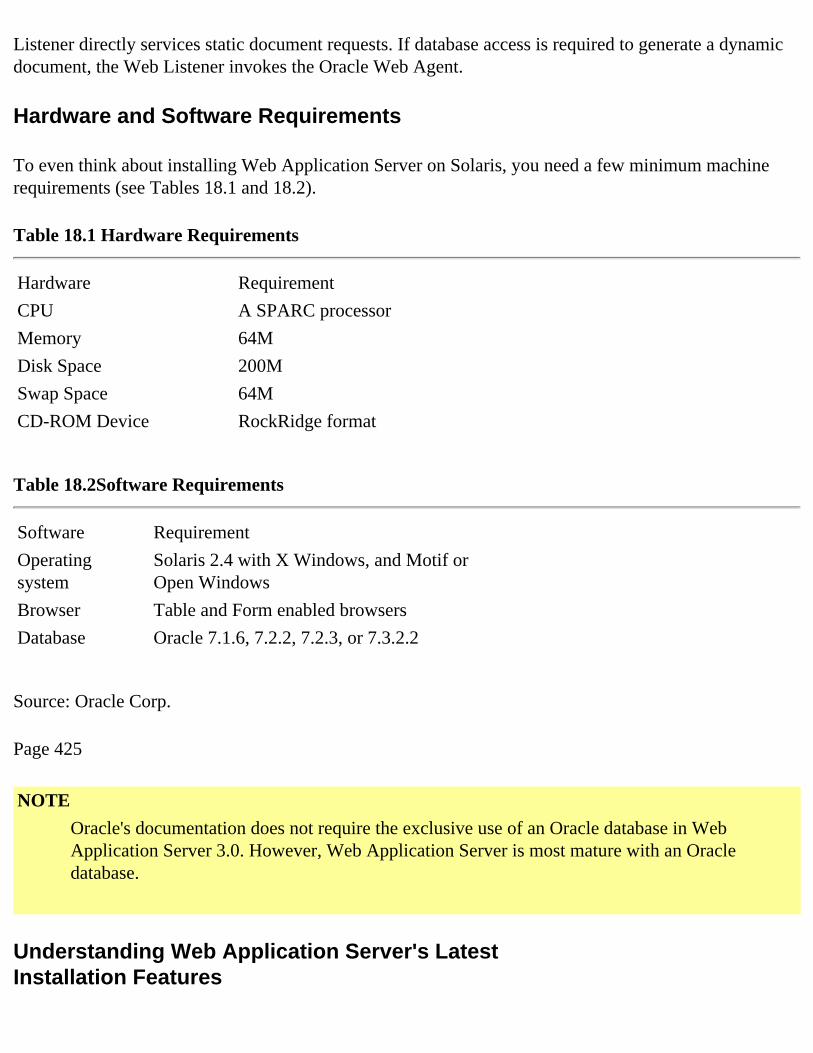
Listener directly services static document requests. If database access is required to generate a dynamic document, the Web Listener invokes the Oracle Web Agent.
Hardware and Software Requirements
To even think about installing Web Application Server on Solaris, you need a few minimum machine requirements (see Tables 18.1 and 18.2).
Table 18.1 Hardware Requirements
Hardware Requirement
CPU A SPARC processor
Memory 64M
Disk Space 200M
Swap Space 64M
CD-ROM Device RockRidge format
Table 18.2Software Requirements
Software Requirement
Operating system
Solaris 2.4 with X Windows, and Motif or Open Windows
Browser Table and Form enabled browsers
Database Oracle 7.1.6, 7.2.2, 7.2.3, or 7.3.2.2
Source: Oracle Corp.
Page 425
NOTE
Oracle's documentation does not require the exclusive use of an Oracle database in Web Application Server 3.0. However, Web Application Server is most mature with an Oracle database.
Understanding Web Application Server's LatestInstallation Features

To help make your installation a little easier, Oracle has incorporated several installation enhancements to Web Application Server 3.0. These features include the following:
● Installation Components—Oracle provides several installation products, including Listener 2.1, Advanced/Basic Web Request Broker 3.0, Cartridges, and Web Request Broker Listener Dependencies.
● The owsctl Utility—This utility provides centralized control of each of Web Application Server's listeners and related Object Request Broker (ORB) processes. After you install the server, run this utility if you plan to use Web Application Server right away. Running this utility initializes a Web Listener.
● Flexible Upgrading and Migrating Options—If your previous Internet server was Web Application Server 2.x, Web Application Server now helps ease your migration migraines. If it was a Netscape Internet server, Web Application Server can also help. However, unfortunately, it does not look like it offers any assistance with migrating from Microsoft's Internet Information Server.
● Single or Multi-Node Install Options—If your domain requires only one network node, you can choose the Single-node option. If more than one, you have the flexibility to customize the install to recognize more than one node.
● Flexible Web Application Server Location Variable (ORAWEB_HOME)—With previous versions of Web Application Server (formerly known as WebServer), the location of the system was tied to the home location specified in the ORACLE_HOME environment variable. In version 3.0, you can now have a location that is not tied to this environment variable. Each installation, then, would have its own environment domain called ORAWEB_HOME.
Relinking Your Executables After Installation
In addition to hardware and software requirements, you might find it necessary to relink your executables. Linking is the process of combining compiled programs and libraries into an executable program. Relinking an executable is necessary because Web Application Server handles some of the duties an operating system would normally handle. In addition, Web Application Server has its own header files that you need to incorporate into any executables that require the services of the Web Server. Keep in mind, also, that the Oracle Web Application Server Option requires the relinking of your executables. Nevertheless, if you choose to relink
Page 426
the executable after doing the installation, Web Application Server requires that you install the following files, libraries, and utilities:
● Oracle library files. These files have the .A extension. ● Oracle makefiles. These files have the .MK extension. ● Oracle object files. These files have the .O extension.

● Networking system libraries. ● The ar library manipulation utility. ● The ld utility. ● The make utility. ● X libraries. ● Motif libraries.
It might be in your best interest to do a full recompile of your executables if time permits. That way, you can isolate any upgrade/migration-related anomalies before they come back to haunt you.
Identifying Product Dependencies
You need to consider what products you must have in place for Web Application Server to be useful. If you plan to use Web Application Server only as a stand-alone Internet server, you don't need to concern yourself with this section. However, if you plan to implement Web Application Server as a server within your overall Oracle environment, you should read the list in this section. To make sure your environment has all of the necessary components, you should go through the following list, which includes the software component and its respective release:
● Oracle7 Server, 7.1.6 ● PL/SQL, 2.1.6 ● SQL*Net, 2.1.6 ● TCP/IP Protocol, 2.1.6 ● Server Manager, 2.1.3
Implementing Pre-Installation Tasks
Before installing Web Application Server for Solaris, you must perform some duties to ensure a smooth installation process. These duties include the following:
● Choose a network port for the Oracle Web Listener. This port number makes it possible for the Web Listener to receive incoming client requests. The number should be at least 1,024 but no higher than 65,535. The default, as installed, is 8,888.
Previous | Table of Contents | Next

Previous | Table of Contents | Next
Page 422
PL/SQL Agent has made improvements since earlier versions of Web Application Server. This improvement comes from the fact that each PL/SQL Agent instance stays connected to your Oracle7x database between incoming requests. The idea here is that there's no need to establish a new database per stored procedure execution. You should use the latest version of PL/SQL after doing isolation testing to make sure that you experience no side effects.
The PL/SQL Agent executes two tasks that allow your stored procedures to create dynamic HTML pages:
● It invokes a parameterized procedure and passes in the essential parameters shipped with the HTTP request. The Web Application Server must perform a translation of an HTTP request to PL/SQL.
● It provides a method for your stored procedure to send data as returns to the caller. The low-level details here are seamless to you.
In addition to performing these tasks, the PL/SQL Agent includes the PL/SQL Web Toolkit—a collection of packaged procedures, functions, and utilities to enhance productivity and ensure valid HTML output.
Previous | Table of Contents | Next

Previous | Table of Contents | Next
Page 418
If chunkSize ub4 has a non-zero value, the size of the request response in bytes will be restricted to this value. In such situations, you'll need to invoke the WRB_ICXfetchMoreData() method repeatedly until you've received the entire response. If ub4 chunkSize is zero, no data is returned. If ub1 sendToBrowser is non-zero, WRB will send the response directly to the originating browser; in this case, the response parameter will contain NULL on return.
WRB_ICXsetAuthInfo()This method sets the authentication header data to accompany the specified request (see Listing 17.13).
Listing 17.13 Setting the Authorization Header for a Specific Request with WRB_ICXsetAuthInfo()
WAPIReturnCodeWRB_ICXsetAuthInfo(void *WRBCtx,dvoid * hRequest,text *username,text *password,text *realm);ParametersReturn ValuesWRB_ICXsetAuthMethod() returns a value of type WAPIReturnCode.
If your cartridge issues requests to another cartridge that in turn requires that your cartridge authenticate itself, you should invoke the WRB_ICXsetAuthInfo() method. Doing so sets the authentication header data per request to the other cartridge.
*WRBCtx is a pointer to the opaque WRB context object that the WRB application engine passed to your cartridge method. dvoid * hRequest identifies the request for which authentication is to be established. WRB_ICXcreateRequest() returns this handle. text * username is a pointer to a user name for request authentication. The user name must be defined in the specified realm. text * password points to the password for the username. text * realm points to the name of the authentication realm that defines the username.
WRB_ICXsetContent()WRB_ICXsetContent() sets request content for a specified request (see Listing 17.14).
Listing 17.14 Setting Content Data for a Specific Request with WRB_ICXsetContent()

WAPIReturnCodeWRB_ICXsetContent(void *WRBCtx,dvoid * hRequest,WRBpBlock hPBlock);ParametersReturn ValuesWRB_ICXsetContent() returns a value of type WAPIReturnCode.
Page 419
To establish content data for a particular request, perform the following steps:
1. Invoke WRB_createPBlock() to allocate a parameter block containing the content data. 2. Pass the parameter block to WRB_ICXsetContent(). You specify the request by passing the
request handle returned by WRB_ICXcreateRequest(). 3. Set the content data.
*WRBCtx points to the opaque WRB context object that the WRB application engine passed to your cartridge function. dvoid * hRequest identifies the request for which content is to be specified. This should be a handle returned by WRB_ICXcreateRequest(). WRBpBlock hPBlock represents the parameter block containing the request content.
WRB_ICXsetHeader()WRB_ICXsetHeader() is responsible for setting HTTP header data for a specified request (see Listing 17.15).
Listing 17.15 Setting Headers for a Specific Request with WRB_ ICXsetHeader()
WAPIReturnCodeWRB_ICXsetHeader(void *WRBCtx,dvoid * hRequest,WRBpBlock hPBlock,boolean useOldHdr);ParametersReturn ValuesWRB_ICXsetHeader() returns a value of type WAPIReturnCode.
Invoking this method requires certain calls having been made first. The sequence of calls involved are as follows:
1. Invoke WRB_createPBlock() to allocate a parameter block and contain the header data. 2. Pass the parameter block to WRB_ICXsetHeader(). You specify the request by passing the
request handle that WRB_ICXcreateRequest() returned.

3. Set header data for a request.
*WRBCtx points to the opaque WRB context object that the WRB application engine passed to your cartridge function. dvoid * hRequest identifies the request for which headers are to be set. WRB_ICXcreateRequest() returns the dvoid * hRequest handle. WRBpBlock * hPBlock represents the parameter block that contains the header information. If boolean useOldHdr is set to TRUE, the ICX request incorporates header data from the original request, in addition to the data defined by the parameter block. If useOldHdr is FALSE, only header data from the parameter block is used.
WRB_ICXsetMethod()WRB_ICXsetMethod() is responsible for setting the request method, such as GET or POST, for a specified request (see Listing 17.16).
Page 420
Listing 17.16 Setting the HTTP Method to Use in a Specific Request with WRB_ICXsetMethod()
WAPIReturnCodeWRB_ICXsetMethod(void *WRBCtx,dvoid * hRequest,WRBMethod method);ParametersReturn ValuesWRB_ICXsetMethod() returns a value of type WAPIReturnCode.
The assumption here is that you invoked the WRB_ICXcreateRequest() method to create a request. Invoke WRB_ICXsetMethod() to specify a request method for the request. The default request method is GET.
*WRBCtx points to the opaque WRB context object that the WRB application engine passed to your cartridge function. dvoid * hRequest identifies the request for which the method is to be set. WRB_ICXcreateRequest() returns this handle.
WRB_ICXsetMethod() takes an argument of type WRBMethod that represents the request method to be used for a request (see Listing 17.17).
Listing 17.17 The WRBMethod Enumerated Type
typedef enum _WRBMethod{OPTIONS,GET,HEAD,

POST,PUT,DELETE,TRACE} WRBMethod;
For more information on this enumerated type, refer to your documentation on Web Request Broker.
WRB_ICXsetNoProxy()This method builds a list of DNS domains for which the proxy server (specified by WRB_ICXsetProxy()) shouldn't be used. This ensures that any request URLs originally intended for the given proxy server are rejected. Listing 17.18 shows how to implement this method.
Listing 17.18 Specifying Domains for Which the Proxy Server Shouldn't Be Used with WRB_ICXsetNoProxy()
WAPIReturnCodeWRB_ICXsetNoProxy(void *WRBCtx,
Page 421
text *noProxy);ParametersReturn ValuesWRB_ICXsetNoProxy() returns a value of type WAPIReturnCode.
If your cartridge calls WRB_ICXsetProxy() to set up proxy server request translation but you don't want requests to all DNS domains to use the proxy server, use WRB_ICXsetNoProxy() to specify a comma-separated list of domains to which requests should be sent directly, without proxy server intervention.
*WRBCtx points to the opaque WRB context object that the WRB application engine passed to your cartridge function. *noProxy points to a comma-separated list of DNS domains to which requests should be sent directly.
WRB_ICXsetProxy()This method tells cartridges which proxy server to use in making future ICX requests that must be routed outside a firewall. Listing 17.19 shows how to specify a proxy server.
Listing 17.19 Specifying a Proxy Server with WRB_ ICXsetProxy()
WAPIReturnCodeWRB_ICXsetProxy(void *WRBCtx,text *proxyAddress);Parameters

Return ValuesWRB_ICXsetProxy() returns a value of type WAPIReturnCode.
Invoking this method is useful when your intranet-based cartridge needs to dispatch ICX requests to servers outside the firewall. The cartridge would reference the address set by this method.
*WRBCtx points to the opaque WRB context object that the WRB application engine passed to your cartridge function. *proxyAddress represents the proxy address in character-string form.
Using the PL/SQL Agent
With the PL/SQL Agent, you can develop your Web applications by using Oracle7x stored procedures. The assumption here is that these stored procedures are written in Oracle's native SQL language, PL/SQL. For non-Oracle databases, you'll have to acquire a third-party ODBC cartridge or develop one yourself. Oracle, however, assures its customers that interacting with database objects is much easier in PL/SQL than any other language. Quite obviously, because Web Application Server is more mature with Oracle databases, your safest bet for portability and scalability issues is to incorporate PL/SQL.
The PL/SQL Agent shares a similarity with its sister, the Web Agent, which was discussed briefly earlier. Both agents allow your development staff to build data-driven, dynamic HTML pages with customized content by using Oracle7x stored procedures. In terms of speed, the
Previous | Table of Contents | Next

Previous | Table of Contents | Next
Page 427
● On UNIX, you must set the following environment variables: ORACLE_TERM, ORACLE_HOME, ORAWEB_HOME, and ORACLE_SID. You also need to know the name of your machine. This is the machine name you normally use to access files and services. For instance, for HTTP Web machines, your machine name might be www.samsona.com or something similar. If you're not sure, ask the person responsible for creating domain names and assigning TCP/IP addresses in your company or group.
● You need patch 101945-27 if you need to install the Oracle Web Application Server option on SUN Solaris. Contact Oracle at http://www.oracle.com.
● Create your admin password. The Installer program asks for a password. You also need to create what's called a root user account to actually have ownership over the Web Listener's UNIX account. A root user account has low-privileged UNIX access, meaning your Web Listener does not need to be tied to a particular DBA group or have Oracle account privileges. Such access compromises your database security. There's a useradd command to help you create such an account for your Web Listener.
The following installation duties require that you log on using the built-in Oracle user account. Because it is assumed that you are an administrative user with the authorization to install such a system, no password is necessary.
Setting Preliminary Environment Variables
Specifying initial values for your server environment variables helps your operating system communicate with Web Application Server. You need to place the necessary environment variable values in the startup file of the built-in Oracle account. This is advisable when possible. Of course, if you don't set them in the startup file, then specify the values in the .PROFILE or .LOGIN file of the Oracle account. You can also set variables specific to the current shell session as the shell prompt is displayed (see Table 18.3).
Table 18.3 Initial Environment Variable Values
Environment Variable
Sample Value
ORACLE_HOME /u01/app/oracle/product/732
ORACLE_SID MyID
ORACLE_TERM xsun5
ORAWEB_HOME $ORACLE_HOME/ows/3.0

PATH
.$ORAWEB_HOME/bin:$ORACLE_HOME/bin: /opt/bin:/bin:/usr/bin: /usr/ccs/bin:/GNU/bin/make
TMPDIR /var/tmp
TWO_TASK Must be undefined while installing software
Page 428
For instance, you set the ORACLE_SID value using C shell as follows:
setenv ORACLE_SID MyIDIn Bourne, it would be the following:ORACLE_SID=MyID; export ORACLE_SID
Setting Permission Codes for Creating Files
You set permission codes in the startup files. The umask variable holds the necessary permission code you need. Before changing the value of umask, look at its contents by entering the following at the prompt:
$ umask
If the value of umask is not 022, change it to this value. This value tells the server which groups or users have READ and EXECUTE permissions; the WRITE permission is not affected. To set umask to 022, do the following:
● For Bourne or Korn shell, enter umask 022 in .profile. ● For C shell, enter umask 022 in .login.
Finally, you should check the various user startup files just to be sure the umask variable is set to 022.
Updating Your Environment from a Startup File
As your environment situation changes (that is, you install new nodes and so on), you will have to upgrade your environment information. To update environment variables, load the startup file into memory or some persistent medium, as follows:
Bourne/Korn shell: $ . .profile

C shell: % source .login
Note that, if you update these variables in a nonpersistent media such as memory (at the prompt), their values are not stored after you exit your current shell session. If you store them in a persistent object such as a file, you must execute the startup file to make the values effective.
Designing the Directory Structure
Identifying your needs for a directory structure in some ways resembles the principles of object-oriented design. You must know your base objects and any derived objects descending from this base object. Implementing the wrong hierarchy can cause confusion later and lead to redundant effort. For directories, this is especially true when server software upgrades become necessary as older versions become archaic. Many domains have a policy in place for
Page 429
creating and maintaining complex directory structures. Oracle offers the Optimal Flexible Architecture (OFA) to ease the management and maintenance duties associated with directories. Listing 18.1 shows the recommended directory structure for the primary node.
Listing 18.1 Oracle-Recommended Directory Structure
ORACLE_BASE product oracle 7.3.2 ($ORACLE_HOME) rdbms ows cartx plsql 1.0 java 3.0 bin lib
admin MyDBName ows MySite1

httpd_MyMachine1 owl.cfg admin config log list80 cartx plsql config log java wrb config log
This directory structure conforms to the Optimal Flexible Architecture directory structure. OFA separates data files from configuration files and executables so that you can run more than one version of any of Oracle's products, including Web Application Server.
Installation Notes on the Web Agent
The Web Listener invokes the Oracle Web Agent. This is the process that handles the details of making a connection to the database server. For installation and configuration purposes, you might want to keep in mind that the Oracle7x database could reside on the same node as the Web Listener and the Web Agent. It could also reside on a different node. However, Oracle requires that the Web Listener and Web Agent be on the same node.
Page 430
As an administrator, you want to properly install and configure the Web Agent and subsequently maintain it by using the Administration Utility. In addition, you need to know the following:
● How to manage Oracle Web Application Server services, including the ability to create, modify, and delete them. Oracle has added several packaged API wrapper classes to help you in this regard, including oracle.owas.wrb, oracle.owas.wrb.services.http, oracle.owas.nls, and oracle.owas.wrb.services.logger.
● On which machine and directory to install the Developer's Toolkit PL/SQL packages provided by the Web Agent. Proper licensing issues come into play here. You need to survey the various developers to discover which directories will house the installation.
● How to set the Web site environment variable. The Oracle Web Application Server needs to know which Web site maps to which server. Oracle Web Application Server 3.0 allows you to have multiple servers per installation. This means you can have multiple Web sites (intranets, for

instance) within a company. You need to set the ORAWEB_SITE environment variable before invoking the owsctl command.
One of the most important installation items you need to create is the OWA.CFG file. In this file, you enter the information the Web Agent needs to connect to your database server, such as Oracle7x. The configuration file contains such vital connection information as the server name, database name, user name, and user password.
Because the Oracle Web Application Server follows Oracle's Flexible Architecture (OFA), configuration files such as the OWA.CFG file no longer have to be located in the OWS Administrative directory. The caveat is that you must have installed your Oracle database according to this OFA structure as well. If this is the case, simply choose the Install New Product option from within the installation program. By choosing this installation option, the Oracle Web Application Server generates each of the necessary configuration files for you within ${Oracle Base}/admin/ows directory, where {Oracle Base} is the base specified in the ORACLE_BASE environment variable. Oracle Web Application Server requires you to specify a meaningful value after the installation is complete.
If you did not install your Oracle database based on the OFA structure, don't worry. Instead of choosing Install New Product, choose Add, Upgrade Software. By choosing this option, Oracle Web Server's installation program creates the necessary default configuration files within the ${ORACLE_HOME}/ows/admin/ows directory. For each new directory structure, every listener has a corresponding listener directory within the following path: ${ORAWEB_ADMIN}/ows/${ORAWEB_SITE}/httpd_<machine_name>/ . The WRB-related configuration files are housed in the ${ORAWEB_ADMIN}/ows/${ORAWEB_SITE}/wrb/ directory.
The Web Agent determines which service to use by parsing the SCRIPT_NAME environment variable. Web Listener sets up this variable in accordance with the CGI 1.1 specification. The path section of the configuration file, which corresponds to the portion of the URL just before the /owa, indicates the service to use. For instance, if /ows-bin/hr/owa is the leading portion of the URL, then hr is the service to use.
Previous | Table of Contents | Next

Previous | Table of Contents | Next
Page 431
Inside the OWA.CFG File
The following section provides an example of a Web Agent service entry in the OWA.CFG file. A description of each variable follows:
Developer's T#(owa_service = es(owa_user = www_samsona)(owa_password = strong)(oracle_home = /home/Oracle7x)(oracle_sid = samsona22)(owa_err_page = /samsona_err.html)(owa_valid_ports = 8000 8888)(owa_log_dir = /home/Oracle7x/ows/log)(owa_nls_lang = AMERICAN_AMERICA.US7ASCII))
Table 18.4 describes each item in the file. You need to specify values in these variables after installation, but before running Web Server.

TIP
Never rely on Web Application Server default values. This is important because the default values are not likely to be suited to your environment. For instance, your home directory most likely would be /home/Oracle7x. Also, for security reasons, you'll use a different ID and password than the defaults.
Table 18.4O WA.CFG File Variables
Variable Description
OWA_SERVICE Name of the Web Agent service.
OWA_USER Database username that the Web Agent uses to connect to the database.
Continues
Page 432
Table 18.4 Continued
Variable Description
OWA_PASSWORD Database password that the Web Agent uses to connect to the database.
ORACLE_HOME
The location of the Oracle7x code tree in the file system. This should be the ORACLE_HOME for the database to which this Web Agent service connects, unless the Web Agent service is set up to connect to a remote database (over SQL*Net). In that case, specify the ORACLE_HOME where the Web Agent is installed.
ORACLE_SID Name of the database system ID to connect to. Does not apply for connections to a remote database.

OWA_ERR_PAGE
HTML document returned by the Web Agent when an error occurs in the PL/SQL procedure that the Web Agent invoked.
OWA_VALID_PORTS The valid Web Listener network ports that the Web Agent will service.
OWA_LOG_DIR
The directory to which the Web Agent writes its error file. The name of the error file is SERVICE_NAME.ERR.
OWA_NLS_LANG
The NLS_LANG of the Oracle7x database to which the Web Agent connects. If not specified, the Web Agent administration program looks it up when Web Listener submits the service. To make sure you've installed the correct version of Web Agent, type $ORACLE_HOME/ows/bin/owa -v at the command line.
Using the Web Administrative Server
The Oracle Web Administrative Server is another Oracle Web Listener process that the Oracle Web Application Server Administrator uses only for its own use. The Web Administrative Server uses a separate Web Agent service for accessing the Oracle7x database. The name of this service is the OWA_DBA service. Thus, in your configuration setup, remember that the OWA_Default_Service is the default service that the Oracle Web Agent uses.
Installing the Oracle Web Application Server Option
To install the Web Application Server option, follow these steps:
1. Start the Oracle Installer. 2. After you have answered initial questions about your database system—preferably the Oracle7x
database—choose to install the Oracle Web Application Server option. 3. Specify the hostname and network port for the Oracle Web Application Server Administrative
Server.
Page 433

4. Specify the password for the Web Application Server Administrator account. The username of the Web Application Server Administrator is admin.
5. On UNIX systems, log in as root and run the $ORACLE_HOME/orainst/root.sh shell script. This step is very important because it initializes and executes the Web Application Server Administrative Server.
Configuring Web Server
The following steps show you how to configure your Web Server. The steps also show how to specify the host name, database name, and other vital pieces of information needed to communicate with other servers, specifically database servers.
To configure your Web Server, follow these steps:
1. Verify connectivity to the Oracle7x database, which is accessed by the Oracle Web Listener. Note that, if the Oracle7x database is on a different node from the Oracle Web Listener and the Oracle Web Agent, SQL*Net has to be installed and configured.
2. Start any Web browser and specify the URL http://HOSTNAME:PORT/ows-abin/register to connect to the Oracle Web Application Server Administrative Server. HOSTNAME is the name of the node where the Oracle Web Application Server Administrative Server is running. PORT is the TCP/IP port used for connecting to the Oracle Web Application Server Administrative Server.
3. After supplying the username and password for the Web Application Server Administrator, complete the Oracle Web Application Server Product Registration Form page and click the Send Registration button. This takes you to the Web Application Server Install Form.
4. Choose to configure the OWA_DBA service and supply the following information: ❍ Username and password for the OWA_DBA Oracle Web Agent service ❍ ORACLE_HOME ❍ ORACLE_SID ❍ Port number of the Oracle Web Administrative Server ❍ SQL*Net v2 service for connecting to a remote Oracle database ❍ Existing DBA username and password
5. Click the Create Service button. This creates the OWA_DBA service. An entry for this service is written to $ORACLE_HOME/ows/admin/owa.cfg on UNIX systems.
6. Choose to configure the first Oracle Web Listener and enter the following information: ❍ Host name ❍ Port Number (note that this should be a different port from the one used by the Oracle
Web Administrative Server) ❍ UNIX user ID and password
Page 434

7. Click the Create Listener button. Clicking this button starts the first Oracle Web Listener. On UNIX systems, configuration information is written to $ORACLE_HOME/ows/admin/svPORT.cfg, where PORT is the TCP/IP port number assigned to the Oracle Web Listener.
8. Choose to configure the OWA_DEFAULT_SERVICE and supply the information required for configuring the OWA_DBA service. Remember that this is the service the Oracle Web Listener will request for non-dba transactions.
9. Click the Create Service button. Clicking this button creates the OWA_DEFAULT_SERVICE service. An entry for this service is written to $ORACLE_HOME/ows/admin/owa.cfg on UNIX systems.
Installing the Web Application Server Developer's Toolkit
Installing the Developer's Toolkit may not be a user-friendly process, but the steps involved provide a good measure of security for your server. These steps ensure that only authorized individuals are installing the toolkit. This also minimizes the risk of bringing down the server. To install the toolkit, do the following:
1. Connect to the Oracle Web Application Server Administrative Server and click the Web Application Server Administration hyperlink. You find the Web Application Server Administration hyperlink on the Oracle Web Application Server Products home page.
2. Click the Oracle Web Agent link. You are prompted for the user name and password of the Web Application Server administrator user. If you're not the administrator, contact that person. This is important because there are settings in Web Application Server that only the administrator knows.
3. Select the service in which you installed the Developer's Toolkit. 4. Scroll down to the button list. In this list, you see the following items:
❍ Create OWA database user ❍ Change OWA database user password
5. Install Web Application Server Developer's Toolkit PL/SQL Package and choose Install Web Application Server Developer's Toolkit PL/SQL Package.
6. Click the Modify button.
Previous | Table of Contents | Next

Previous | Table of Contents | Next
Page 445
CHAPTER 19
Oracle Networking Fundamentals
In this chapter
● Understanding Oracle Networking Product Features 446 ● SQL*Net and Net8 Architectures 448 ● Networking Protocol Stacks 449 ● Using the Open Systems Interconnection Reference Model 451 ● Understanding SQL*Net Operations 456 ● Installing and Configuring SQL*Net 456
Page 446
Understanding Oracle Networking Product Features
Oracle Network Products—SQL*Net in the Oracle7 environment and Net8 in Oracle8—are Oracle's networking solution for transparent client-to-server and server-to-server application connectivity. These products contain a rich core of network services, including data transport, network naming, security, and transaction monitoring. These Oracle Network Products form an abstraction layer, insulating users and user applications from the physical network, allowing heterogeneous, distributed computing across computers regardless of vendor, operating system, hardware architecture, or network topology. Applications will work as written on an AS-400 with LU6.2 network protocol, on a token-ring network, or on an HP-9000 with TCP/IP network protocol on an ethernet network. Oracle SQL*Net is available on virtually every platform supported by Oracle, from PCs to mainframes, and supports almost every network transport protocol, including TCP/IP, Novell SPX/IPX, IBM LU6.2, NetBIOS, DECNet, and AppleTalk.
The Oracle Network architecture offers excellent performance for all it does. In Oracle7, SQL*Net supports network load balancing and fault tolerance. When multiple paths to the database server exist, SQL*Net determines which route is the most efficient and establishes the connection accordingly. Additionally, during connection setup, SQL*Net will detect any component failures on the primary path and will automatically switch to an alternate route if possible, using secondary network interfaces or network software protocol stacks. SQL*Net will also detect a broken connection and release all server resources, cleaning up failed connections.

Oracle8 and Net8 surpass the SQL*Net family in performance and scalability through two new features: connection pooling and session multiplexing. These technologies reduce the amount of server-system resources needed to support network connections, allowing a single database server to support increasing numbers of users. In Oracle8 Enterprise Edition, a new middle-ware application called Oracle Connection Manager takes advantage of the multiplexing feature to act as a high-speed proxy to a database server. As a proxy, Oracle Connection Manager acts as a firewall, controlling network-level access to the database server for enhanced network security.
Other standard features available in all Oracle Network Products:
● Support for multiple protocols running simultaneously on a single machine. ● Support for transaction processing monitors such as Encina and Tuxedo. ● Open interfaces to third-party applications through open interfaces and Oracle's SQL*Net/Net8
OPEN application programming interface. ● Open database interfaces using Oracle's SQL*Net/Net8 Open Database Connectivity (ODBC)
drivers for Microsoft Windows, and Oracle Transparent Gateway technology for third-party database access. Net8 provides interfaces for JavaSoft's JDBC specification for Java applications.
● Multiple protocols in a single connection when using the Oracle MultiProtocol Interchange. The Oracle MultiProtocol Interchange runs on a computer loaded with two or more protocols. This computer provides transparent protocol bridging so clients running one protocol can connect with a server running a different one.
Page 447
Understanding the Administration and Management Components
Oracle Network Products include a comprehensive set of administration and management components. SQL*Net's graphical management facility, Oracle Network Manager for Oracle7 and Net8 Assistant for Oracle8, are powerful tools for creating and managing an Oracle network. Oracle Net8 Assistant supersedes Oracle Network Manager by providing a Java-based tool that is driven by a wizards interface. Using these tools, the administrator can configure all components of the Oracle SQL*Net family, including database servers, gateways, clients, and Oracle MultiProtocol Interchanges, either centrally or in a distributed fashion. Oracle Net8 Assistant runs on most desktop and UNIX operating systems, but Oracle Network Manager is only for desktop systems.
Oracle Names, the Oracle global naming service, is also fully administered and maintained through the above tools. Oracle Names allows administrators to define network entities (such as service addresses, database aliases, and so on).
SQL*Net and Net8 include support for the Simple Network Management Protocol (SNMP). The Oracle7 and Oracle8 servers (as well as Network Listener, MultiProtocol Interchange, and Oracle

Names) can be monitored by SNMP-based network management consoles, such as Oracle Enterprise Manager and HP OpenView. This allows existing network operation centers in a company to include Oracle systems in their proactive monitoring.
Other administrative components and features include:
● Client registration services give SQL*Net 2.3 and Net8 administrators access to registration information about who is accessing the database, including username and resource usage.
● Comprehensive diagnostic error and trace logging at the client and the server. Oracle Trace in Oracle7 Release 7.3 and Oracle Trace Assistant in Net8 are diagnostic and performance analysis tools to help administrators interpret trace information generated.
● Native naming services allow the application of existing enterprise-wide directory services, such as Sun NIS/Yellow Pages, Novell NetWare Directory Services (NDS), Banyan StreetTalk, and OSF DCE Cell Directory Service. This Advanced Networking Option integrates Oracle clients and servers into the native name environment.
● Network configuration and route testing tools, including Network Test (NetTest), for testing connections to remote databases across the network and TNSPing for testing connections to servers, without need for a service name, username, and password. TNSPing also allows full diagnostic tracing to a trace file and measures round-trip time for the client-to-server connection.
Network Naming Conventions
One of the challenges in a large organization is producing unique names for all network resources. The common flat model naming system, where objects are given a single unique name, often falls short in the enterprise. For this reason, Oracle supports naming network resources using a domain hierarchy. In a domain model, network resources are named according to the group they fall in or the purpose they serve. For example, the marketing department
Page 448
in the Oracle Corporation may belong to the marketing.oracle.com domain. TNS resources belonging to the marketing department would be named using this domain—for example, prod01.marketing.oracle.com for a production database or listener01.marketing.oracle.com for a listener.
In version 7.3 of the Oracle database, TNS resources are placed in the world domain if no domain is created for them. This ensures that network applications expecting a domain name will always have one, even if the organization has implemented a flat naming hierarchy.
NOTE

Oracle tools will expect the full network resource name, including the domain, unless a default domain is specified in the sqlnet.ora configuration file. The names.default_domain parameter specifies what domain should be automatically added to any network resource name when resolving the resource name.n
For most installations, using a flat naming model (implemented with the .world default domain) is sufficient. Adding domains to your network topology should be done out of need, not just because it can be done. Managing an Oracle network with multiple domains adds complexity to the installation and configuration.
Understanding the Optional Security Extensions
The final set of Oracle Network Products includes several optional security extensions that make up the Oracle Advanced Networking Option. These include:
● High speed global data encryption using RSA RC4 or DES encryption algorithms. This encrypts all network traffic with either a 56-bit or exportable 40-bit encryption key.
● Single sign-on using Kerberos and SESAME authentication servers, Security Dynamics ACE/Server token system, and Identix TouchNet II fingerprint ID system.
● Integration with OSF/DCE and the DCE security system.
SQL*Net and Net8 Architectures
With the introduction of Oracle8, Oracle has renamed the current SQL*Net Network Product group to Net8. As mentioned previously, Oracle has introduced some new network performance and scalability features in the updated Net8 product. All other components and features in Net8 remain relatively unchanged from SQL*Net 2.3.3, the latest SQL*Net release for Oracle7 Release 7.3. In this discussion of Oracle networking fundamentals, I will be describing features and functions of SQL*Net 2.3.3. I will also be using the example of TCP/IP and ethernet in most examples, since these are the predominate network architectures. To make things as simple as possible, I will try to define all jargon and use analogies where possible.
In most of the current SQL*Net architecture diagrams, SQL*Net is shown as the central building block, tightly integrating network transport (Oracle Protocol Adapters), network naming (Naming Adapter), and security services (Oracle Advanced Networking Option) at the network level. User-client applications ride on top of this SQL*Net layer to access Oracle7 servers,
Previous | Table of Contents | Next

Previous | Table of Contents | Next
Page 443
PART V
Oracle Networking
19. Oracle Networking Fundamentals 20. Advanced Oracle Networking
Page 444
Previous | Table of Contents | Next

Previous | Table of Contents | Next
Page 442
Previous | Table of Contents | Next

Previous | Table of Contents | Next
Page 449
transparent gateways to third-party database servers, procedural gateways to other applications, or the Oracle Web Server.
Networking Protocol Stacks
In this section, you will look closely at the network transport services, the native local area network (LAN), and wide area network (WAN) protocol stacks that make up the core of networking. You will also touch on native network naming services as they apply to the native network protocols. Native network naming services are used to map "English" names and aliases for computers with their network addresses. Oracle Names is used to map English names and aliases to Oracle databases. Oracle Names often takes advantage of native network naming services by allowing the administrator to specify server host names rather than network addresses in the Oracle Names database.
As promised, jargon will be defined as it comes up, starting with network architectures and protocol stacks. A network architecture is a collection of modular components that are combined to form an effective, synergistic solution. Each component provides a "service" to the whole. By choosing and combining a subset of the available component technologies, a network architecture is built. It is this ability to mix and match components that underlies the principle of open systems and interoperability.
Without some type of reference blueprint for the assembly of components and a set of standards governing their construction, these pieces would not be plug and play. This environment exists for native network transports. These standards are often called protocols, and the reference blueprint is called a stack. The reference blueprint describes the network framework as a stack of service layers, much like a layer cake. Each layer has a specific, clearly defined responsibility within the stack and provides service to the layer above until the stack of components is working together.
For the native network transport, the reference model is the International Organization for Standardization's (ISO) Open Systems Interconnection reference model. Standards are developed and maintained by the American National Standards Institute (ANSI) and the Institute of Electronic and Electrical Engineers (IEEE) 802 committee. The Oracle networking layers and protocols above the native network transport follow Oracle's SQL*Net architecture.
The current SQL*Net architecture blueprint is missing some important protocol layer detail needed to understand how SQL*Net works. It is missing the core network protocol of SQL*Net, Oracle's Transparent Network Substrate (TNS) peer-to-peer networking application. It is the TNS that provides the primary abstraction layer, or a common application interface, to many of the network products that make Oracle applications hardware and network transparent—thus the name Transparent Network

Substrate. TNS provides the service layer to access the native network transport, Oracle Names, and various security and naming services. The Oracle Network Listener is a TNS application that runs on an Oracle server to establish connections between clients and the server. The TNS layer is responsible for most of the client error messages, as the TNS prefix on these error messages reveals.
Page 450
There are five fundamental protocol layers that make up the SQL*Net architecture (see Figure 19.1):
● Network-Specific Protocol Stack: The foundation is the native network transport supported by the computer and the local area (LAN) or wide area (WAN) network. The most commonly used LAN protocol, and the one used in examples, is the TCP/IP protocol stack, though SPX/IPX, NetBIOS, DECNet, LU6.2, AppleTalk, Banyan Vines, MaxSix, Named Pipes, OSI, and X.25 protocols are also supported.
● Oracle Protocol Adapter: The connector between the function calls of the TNS protocol and the native network transport protocol stack. The adapters are specific to the exact native stack used.
● Transparent Network Substrate (TNS): The peer-to-peer networking protocol, very similar to NetBIOS, that forms universal transport for all Oracle network products.
● SQL*Net: Layers on top of TNS to offer a set of functions needed to authenticate and communicate with a distributed database.
● User Programmatic Interface (UPI): Sits on top and is the application programming interface connector between SQL*Net and the client application.
FIG. 19.1The client side andserver side SQL*Netand Net8 protocolstacks.
Oracle Protocol Adapters
The Oracle Protocol Adapters are the interfaces between specific native protocol stack implementations and the Transparent Network Substrate (TNS). The Oracle Protocol Adapters perform a function similar to the interfaces in the native network transport, mapping the standard functionality to TNS with those functions found in the native stack. Oracle Protocol Adapters are specific to the exact vendor's implementation of the native protocol stack.

Transparent Network Substrate (TNS)
As stated earlier, the TNS is a peer-to-peer networking protocol developed by Oracle. It provides the means for establishing network connections and delivering a "pipe" through which to pass SQL*Net, application messages, and data. The most critical TNS application is the Network Listener.
The Network Listener is a protocol-independent application listener, or daemon, that receives TNS connections for any TNS application running on the Oracle server. SQL*Net connections
Page 451
are identified by the listener, based on a SQL*Net-specific port or socket identified in the ADDRESS portion of the connect descriptor in the TNSNAMES.ORA file or Oracle Names database. While a session is established with the listener, a dedicated server process is established (or assigned) to handle the communication session.
Using the Open Systems Interconnection Reference Model
As the foundation for both TNS and SQL*Net, your local area network (LAN) protocols must be working properly before anything layered on top will work. Understanding proper LAN operation, therefore, is a required prerequisite to understanding Oracle networking. As I describe the native network protocol stack, I will emphasize the concepts needed for troubleshooting and proper design.
As previously mentioned, the reference blueprint for the native network transport is the ISO's seven layer Open Systems Interconnection (OSI) reference model. In the late 1970s, the ISO organized a subcommittee of computer professionals to establish standards to encourage interoperability among computer and data communication vendors. The resulting OSI blueprint organizes network communication into the following seven layers:
Layer 1—Physical LayerLayer 2—Data-Link LayerLayer 3—Network LayerLayer 4—Transport LayerLayer 5—Session LayerLayer 6—Presentation LayerLayer 7—Application Layer
For your purposes, this reference blueprint is much too detailed; I will describe a simplified reference blueprint (see Figure 19.2), beginning with the foundation, the interfaces, and the protocol stacks.
The Foundation

Nothing can be built without a strong foundation. The same is true of networks. This layer consists of the physical cabling and electronics required to electrically transmit data between computers. This world is governed by the Electronics Industries Association (EIA), Telecommunication Industries Association (TIA), and the Institute of Electrical and Electronic Engineers (IEEE). The joint EIA/TIA standards committee has worked toward the development of a cabling standards and standard practices. These standards harmonize the wiring necessary for telephone and data. The adoption of the EIA/TIA-568A standard in the wiring industry has driven most LANs to a star-wired design using telephone-type cable called unshielded twisted-pair (UTP). Shielded twisted-pair (IBM Type1 Token-Ring) and fiber optic cabling are also recommended in the 568A standard.
Previous | Table of Contents | Next

Previous | Table of Contents | Next
Page 452
FIG. 19.2The "simplified" 3-LayerReference Modelcompared to the OSIModel.
The IEEE 802 committees set standards for the electronics that push bits over the cabling. It is the Media Access Control (MAC) protocol that defines how bits are pushed onto the network. This software talks directly to the network hardware. For performance and technical reasons, this is a complicated and cryptic interface. The MAC protocol calls for the assignment of unique addresses to individual network adapters so that each computer's network adapter is uniquely addressable, much like a telephone number. This address, called a MAC address, is a 12 digit, hex serial number "burned" into a chip on every network adapter. The first six digits of the MAC address are assigned to each hardware vendor by the IEEE. The last six digits of the MAC address are the serial number set by the vendor.
IEEE standards exist for most of the popular network technologies, including EtherNet, Token Ring, FDDI, 100BaseT, ATM, and Gigabyte Ethernet.
Why should you care about this layer? There are two very good reasons. First, the MAC address (sometimes called the DLC address) is a critical addressing component for almost every protocol stack. Individual workstations can be identified and tracked based on this number. The other reason is that this layer is the most unreliable layer in the network. It is often said that 80 percent of network faults occur in the wiring. These faults are not only due to bad or loose wiring connections. Wiring faults can also be due to wrongly configured electronics.
TIP

With EtherNet, one of the main sources of failure comes from excessive packet collisions. The causes for this can be attributed to an excessive number of repeaters between stations (more than three), EtherNet transceivers connected to repeaters with SQE turned on (SQE should never be turned on in this instance), and failing EtherNet adapters not listening before sending.
The Interface
On top of the foundation is an interface. The main interface for LAN protocols is the IEEE 802.2 Logical Link Control protocol. It creates a simple and standard means, called Service
Page 453
Access Points (SAPs), for accessing the wire. This is not a very important layer for troubleshooting, but you probably should remember that SAPs are the methods used to access the foundation, since this term comes up occasionally.
The Protocol Stack
Above the interface is the protocol stack. The protocol stack encompasses the network and transport layer of the OSI model. Multiple protocol stacks can share the same wire, while the same protocol stack can use different wires. The network layer of the stack handles the routing of messages through the network or through the multiple connected wires. The transport layer of the stack provides error-free transmission of data, data flow control, error recovery, and receipt acknowledgment. TCP/IP has established itself as the standard protocol stack. Other protocol stacks include IPX/SPX, NetBIOS, DECNet, LU6.2, AppleTalk, Named Pipes, Banyan Vines, and so on.
The protocol stack is very complicated. A lot goes on in the stack, and each stack is very different from another. Protocol stacks often have another addressing scheme different from the MAC address. These addressing schemes often break a network up into sub-networks or subnets, also called zones or areas in some stacks. Much like an area code is needed when dialing a long-distance telephone number, special subnet addressing is used to communicate with another subnet. Specialized devices, called routers, are placed at the intersections of adjacent subnets to inspect messages and deliver them to the correct subnet.
The TCP/IP Protocol Stack
TCP/IP is the most popular protocol stack used for SQL*Net and client/server connections. Developed in the 1960s by the U.S. military and a group of west coast American universities, TCP/IP was developed for the original Internet, called the ARPANET. Core to the design of TCP/IP was the ability to "self-heal" in case of the loss of a portion of the network. This was important to a Cold War military

concerned about command-and-control during a nuclear attack. It is also a good design for a huge network without any central control—the Internet.
The TCP/IP stack can run over almost every type of foundation, including EtherNet, Token Ring, Frame Relay, and ATM. This flexibility accounts for much of TCP/IP's success. The TCP/IP protocol implements two protocols, IP and ICMP, to handle the routing of messages through the network.
Internet Control Message Protocol (ICMP) ICMP is a very important protocol for troubleshooting, because it provides error and other control information for testing of routes through a network. Some of the most useful ICMP messages include:
● Echo Request/Echo Reply. A TCP/IP utility called PING uses echo request and reply to determine if a specified address can be reached. The PING command sends an echo request to the remote node. If the protocol stack is working, it will reply to the request with an ICMP echo reply. When PING receives the reply, it will calculate the elapsed time required for the round trip. It will also indicate if a reply is missing, indicating a busy network. This tool is indispensable.
Page 454
● Destination Unreachable. If a route between networks or subnets cannot be accessed, ICMP reports the error. Again, the PING tool will report an unreachable destination, indicating some type of routing misconfiguration or network failure.
● Time Exceeded. ICMP will report back to the sender when the message's time-to-live (TTL) counter expires. The TTL counter is normally set to 20 when a message is first broadcast on the network. Each time a message passes through a router moving from one network or subnet to another, the TTL counter is decremented by one. When the counter is decremented to zero, ICMP sends the message back to the sender providing the name of the last router or hop. This stops messages from getting into infinite loops and provides the name of the offending router.
Another indispensable tool for TCP/IP uses this feature to trace the route a message takes to get to its destination. The TRACEROUTE tool begins by sending a message with a TTL of one. This first router will expire its counter and send back the message. The address of this router is then recorded by TRACEROUTE. A message with a TTL of 2 is now sent to discover the second router, and so on until the destination is found. In Windows 95, this standard Microsoft utility is called TRACERT.EXE.
TIP

A super, free combination PING and TRACEROUTE tool called Sub-O-Tronic is available for Windows 95 from Virgin Interactive at http://subspace.vie.com on their download page. It is a diagnostic tool for use with their SubSpace Internet game to identify network bottlenecks hurting the performance of their client/server game. It works just as well looking for network problems and bottlenecks in your network. A must have!
Another area of concern for most administrators is correct IP addressing and configuration. For the IP protocol to correctly route your messages across the network, several parameters must be set up correctly.
IP Addressing The IP address is expressed in 4-byte, dotted-decimal notation. In decimal notation, a byte can have a value between 0 and 255, so a 4-byte, dotted-decimal notation looks like an address between 0.0.0.0 and 255.255.255.255. As mentioned earlier, the IP address refers to both a specific network or subnet and a specific host. This address is divided into classes.
● Class A—The first byte of a Class A address is a number starting with 1 to 126. Class A addresses use the first byte to designate the network address and the last three bytes to designate the host address. Class A addresses are reserved networks with a huge number of hosts.
● Class B—The first byte of a Class B address is a number starting with 128 to 191. Class B addresses use the first two bytes to designate the network address and the last two bytes to designate the host address. Class B addresses are normally reserved for Internet service providers.
● Class C—The first byte of a Class C address is a number starting with 192 to 223. Class C addresses use the first three bytes to designate the network address and the last byte to designate the host address. Only 254 hosts can be in any Class C network.
Previous | Table of Contents | Next

Previous | Table of Contents | Next
Page 467
CHAPTER 20
Advanced Oracle Networking
In this chapter
● Understanding Enterprise Networking 468 ● Configuring SQL*Net and Net8 468 ● Understanding the Oracle Names Server 475 ● Using the Advanced Networking Option 477 ● Enabling Data Encryption and Checksums 478 ● Understanding the Multi-Threaded Server 479 ● Using the Oracle Connection Manager 483
Page 468
Understanding Enterprise Networking
The Oracle database is capable of supporting many different environments, from small workgroups supporting tens of users and hundreds of megabytes of data, to enterprise applications with thousands of simultaneous users, gigabytes of data, and hundreds of transactions per second. In a similar vein, Oracle networking is designed to support both the smallest and largest environments. If your needs are simple, your Oracle networking components can be configured so that one person can easily administer them with a minimum of time and effort. For larger installations with more complex implementations, the same concepts used in a small installation can be built on and expanded to support more challenging requirements. In this chapter, you look at some of the features of SQL*Net and Net8 that enable it to serve the needs of the enterprise.
Configuring SQL*Net and Net8
Unfortunately, installing the SQL*Net networking software is the least of your Oracle networking administrative duties. SQL*Net software must be carefully configured before it can be used, both on client and server machines. There are, in general, two accepted methods of configuring SQL*Net—through manual editing of the correct configuration files, or through the usage of the supplied Oracle configuration tools, Network Manager for Oracle7 and Net8 Assistant in Oracle8.

Oracle recommends configuration of the SQL*Net configuration files only through the supplied configuration. However, experienced (or impatient!) network administrators are often more comfortable making configuration changes directly to the configuration files. Also, there are times when the only way to configure a brand-new networking product, or enable a feature, is through direct configuration file manipulation. For these reasons, it is highly recommended that you at least familiarize yourself with the configuration files involved in SQL*Net and Net8 communication.
NOTE
Currently, the Network Manager and Net8 Assistant utility will not edit configuration files that have been modified by hand. Therefore, you must make the choice to either use the tool, or not to use the tool.
The easiest and most foolproof way to configure SQL*Net is with the Network Manager utility. In most cases, configuring your network resources using the Network Manager or Net8 Assistant is simply a matter of choosing the appropriate icon and filling in a few parameter values. The way these tools work is that the network configuration is stored internally. Based upon the Oracle resources you have created (such as Listeners, Names Servers, Databases, and so on), the appropriate configuration files for clients and servers are generated when you execute the utility. You are then responsible for placing these generated configuration files in the appropriate directories on the client or server.
The Net8 Assistant is different from Network Manager in that it is a Java application, and as such can run on any platform that has the appropriate Java runtime environment installed.
Page 469
It also contains additional functionality not found in Network Manager, as well as support for new Net8 features, such as the Connection Manager and the Advanced Networking option.
Using the Oracle Tools to Configure Oracle Networking
The following step-by-step explanation will create a simple Oracle network using the Network Manager tool. We will create a Oracle network consisting of a database server, a Listener, a database, and a Names server. Note that placing your mouse cursor over a button will cause a message explaining the button's purpose to appear. All of the button's functionality can also be performed using menu items. Complete the following steps:
1. Start the Network Manager utility. With some versions, you will be asked where you would like to store the Network Definition: Select File.
2. Select File, New, or press the Create A New Network Definition button. The utility will ask whether you want to perform a walk-through; select No.

3. Press the Community button, and enter a name for the community. In Oracle terms, a community is one or more network resources that use the same protocol, and the community name should reflect the protocol name. Choose the correct protocol from the Protocol drop-down list, and press OK. Notice how each component of the network appears in the box at the left of the Network Manager screen as you create it, and the network resources contained within each highlighted container object appear in the box at the right.
4. Press the Node button. A Node is a computer that houses an Oracle resource, such as a database or listener. Enter the name of the Node (the computer name), and select the Node type from the Node drop-down list. You will also need to select the community the Node belongs to by selecting the Community tab and adding the correct Community.
5. Press the Listener button. As you can see, the Listener has many configurable options, but most of them are related to optional behavior, such as logging levels and monitoring. The name will default to Listener, and unless there are multiple listeners for the server, there is no need to change this value. The first Node will automatically appear in the Node box; select the correct Node if necessary. You can also assign a password to the Listener, which will be used when attempting to perform administrative tasks on the Listener. For now, the other parameter values can be left at their defaults. b. Select the Addresses tab. The address will specify the hostname and port on which the Listener will listen at. The default is 1521 or 1526, depending on the server type, and in most cases the default is fine. Press the Create button and accept the default values by hitting OK.c. Select the Databases tab. Here you specify what databases the Listener will listen for. You can only specify databases that reside on the Node the Listener resides on. If you have databases already created, you can select them from the Available list. Otherwise, press OK to create an empty Listener. We will assign databases to it in the next step. One quirk of Network Manager is that you cannot create databases on a Node without first creating a Listener on that Node.
Previous | Table of Contents | Next

Previous | Table of Contents | Next
Page 466
Previous | Table of Contents | Next

Previous | Table of Contents | Next
Page 463
To install specific product components, double-click the desired product in the Products Available list and then select the specific component to install. Click Install to begin product installation.
TIP
Update the Windows Registry to add the key USERNAME to the HKEY_Local_Machine/Software/Oracle section and the HKEY_Local_Machine/Software/Oracle/Oracle_Homes/Oracle1 section. The value for this key should be the user's name. This value is used when a SQL*Net connection is made to the Oracle server. This value is displayed on the server for your connection. This will aid releasing connections to shutdown the database.
TIP
Two other changes to the Registry should be considered. Add the key CNTL_BREAK=ON to the HKEY_Local_Machine/Software/Oracle and HKEY_Local_Machine/Software/Oracle/Oracle_Homes/Oracle1 sections of the Windows Registry. This key will allow a Ctrl+C keypress to stop a long query. Also, changing the value for NLS_LANG in both sections can improve the order data is sorted using the ORDER BY clause. PeopleSoft software running against Oracle requires the US7ASCII character set be used. Use the following syntax in the ORACLE.INI file: NLS_LANG=AMERICAN_AMERICA.US7ASCII.
Using The Oracle Client Software Manager (OCSM) Component
Oracle Client Software Manager (OCSM) is a new feature to the Oracle Windows Installer. It allows the administrator to install 16-bit applications on a shared file server directory for use by any Windows client platform, including Windows 95 and Windows NT. Installation is centralized and updates to software on client workstations are automatic, using the intelligence built into Oracle Installer.
The Oracle Client Software Manager can be used to deliver 16-bit client software bundled with Oracle7 Workgroup and Enterprise servers including SQL*Net. Runtime and development versions of Oracle Developer/2000, Oracle Office, and the Oracle Applications suite can also be installed with OCSM. It is also a critical delivery tool for the GUI version of Oracle Financials.

CAUTION
Two notable omissions to the applications delivered by the Oracle7 OCSM is the Oracle ODBC driver and the 7.1 and 7.0 Required Support Files. This is no longer the case with Net8.
Oracle Windows Installer creates the Oracle Client Software Manger directory and loads the selected software into this shared network directory. Oracle Windows Installer configures the administrator's PC to run the Oracle Client Software Administrator, a utility that allows the administrator to set up client configurations. The exact suit of products needed by a group of users is associated to a configuration. Users are then assigned the appropriate configuration to perform their job. Optionally, the administrator can give the user a suite of products to pick from and install for himself.
Page 464
The Client Software Administrator has other options such as installation conflict resolution and the ability for the administrator to decide the location of executables. A client can be configured to use Oracle applications in three ways.
● In shared mode directly from the file server ● In EXE/DLL download mode when just the executables and DLLs are loaded locally on the
client PC for performance improvements ● In Full Download mode, when a complete installation is made on the client machine
The user portion of OCSM is the Oracle Client Software Agent. This small executable is loaded onto the client PC and is run in the Windows Startup group. The Agent monitors the server for changes and automatically updates the client using the Oracle Window Installer engine.
Installing SQL*Net Using the Oracle Client Software Manager
If you are running Windows 95 or Windows NT, your PC will probably autorun the installer for the appropriate 32-bit version of SQL*Net for your operating system. Since you are installing, and OCSM only works with the 16-bit version of the Oracle Network Products, cancel out of this installation if autorun is enabled on your PC. Use the following steps to install SQL*Net using the Oracle Client Software Manager:
TIP
Autorun can be disabled by holding down the Shift key while loading the CD-ROM.

1. Start the Oracle Installer. The install directory on the CD-ROM for the 16-bit version of Oracle Network Products is called \WINDOWS. Change to this directory. Find and run the program SETUP.EXE with a /SHARED option using File, Run in Windows 3.1 and Windows NT 3.51 or the Start/Run dialog in Windows 95 and Windows NT 4.0. Type in the following (substituting your CD-ROM drive letter for D): D:\WINDOWS\SETUP.EXE /SHARED.
2. Select Oracle Installation Settings. 3. Next you will be prompted for the language being used for the installation. After choosing a
language and selecting OK, you will be presented with an Oracle Installation Settings dialog box. Type your company name in the Company Name field, and then specify the location of the shared Oracle home in the Oracle Home field.
CAUTION
You must be careful in specifying the Oracle home for the shared installation. This path should be on a network file server drive that all Oracle users can access. This should NOT be on your local hard drive.
4. You will then be prompted for the /BIN directory setting in your Autoexec.bat file. You will see the Oracle Client Software Manager Administrator Information dialog box. Type in the administrator's username, and click OK. The standard Software Asset Manager dialog box will now appear.
Page 465
5. Install the Oracle Installer, Oracle Client Software Manager Administrator, and the Oracle Client Software Manager Agent to the shared Oracle home by first highlighting them on the left pane and clicking Install. Once complete, install all other required applications, such as SQL*Net and the appropriate Oracle Protocol Adapter. Pick any other applications needed in the shared Oracle home.
6. Exit the Installer.
As the Software Manager Administrator, the Administration program will be installed on your PC. You will need to use the PC to make changes to the shared configuration.
CAUTION
You cannot be the Software Manager Administrator AND a user running the Manager Agent. You probably should pick a machine you do not use for development or production as your Administrator machine. You should pick an alias name as your administrator name so it will not conflict with your username if you install Oracle products on the computer at your desk.

Previous | Table of Contents | Next

Previous | Table of Contents | Next
Page 470
6. a. Now that the server and Listener are configured, we are ready to create a database entry. Press the Database button, and fill in the Database Name, Node, and Database SID fields. Set the Database Name to the name you specified when the database was created (or the value of the db_name init.ora parameter). Also fill in the Operating Specific directory in the field, if necessary.
NOTE
Step 6a does not actually create a database. It only defines it within the SQL*Net environment.n
b. Press the Listeners tab, and select the Listener(s) that will service this database from the list of Available Listeners. You cannot create the database without specifying a Listener. Press OK to accept the default settings for all other configuration parameters.
7. Select File, Validate. This will ensure all of your object definitions have been properly created. 8. Select File, Generate. If this is a new configuration, you will be asked to provide a network
definition filename. You will also be prompted for the directory in which to store the generated network configuration files. Select a directory, and press OK.
After generation has completed, the configuration files for the Oracle network will be in the directory you specified in the last step above. A directory exists with the name you gave the network file. Within this directory will be subdirectories for each Node in the network, as well as for each community. The community directory will contain the files necessary for clients, and the server directories will contain the server configuration files. Transfer these files to the appropriate directories on the server or clients, and test your network configuration. Assuming all parameters were entered correctly, your networking configuration is complete.
When a change is made to the network configuration, it will be necessary to regenerate and distribute all of the configuration files for each server. While time-consuming, the benefits you realize from maintaining the entire network configuration in one central location are great.
NOTE
Network Manager and Net8 Assistant store the options found in the sqlnet.ora file in the Profile object. Edit the Profile for the Community to modify the sqlnet.ora parameters.n

Creating a network configuration using Net8 Assistant is very similar to doing so with the Network Manager. The biggest difference is the look and feel of the utility itself. Terminology and configuration is for the most part identical, with the addition of configuration for Net8 resources and options. The new configuration options available in Net8 are detailed in the following section, "Exploring the New Net8 Parameters."
Exploring the New Net8 Parameters
One of the most noticeable differences between Net8 and SQL*Net V2 are the new configuration parameters available. The following is a list of the new parameters you should be aware of (most of these parameters can be configured in the Profile editor in the Net8 Assistant, or by hand by editing the sqlnet.ora file):
Page 471
DISABLE_OOB—Disable out-of-bound breaks if transport protocol doesn't support a feature. Out-of-bound breaks are what allows you to cancel a long-running query or job by pressing Ctrl+C (or the Cancel button), by sending a control command that does not wait for completion of the current command, but executes immediately (in other words, an out-of-bound command).
SQLNET.EXPIRE_TIMEOUT—In earlier versions of SQL*Net, this defaulted to an extremely high number of seconds. When calculated, it measures in years. It is recommended that this value be reduced to a more manageable number, such as 10. This does not mean that if the connection is idle for 10 seconds, it will be disconnected, but rather when the connection dies it spins off on its own. This is the number of seconds the process will stay active prior to being killed. DBAs that have had to deal with locks left over from these "ghost" processes will appreciate the effects of this setting.
LOG_FILE_CLIENT—The log file will be written on the client to this filename. The file will be placed in the directory specified in TRACE_DIRECTORY_CLIENT. Logging is automatic in Oracle and cannot be turned off. It tracks the errors that occur on the client. This is a good place to go when evaluating errors. When not specified, the default filename is SQLNET.LOG. This file should be periodically purged; however, this should be done while the client is quiet so that the logging facility will find the file if an error occurs.
LOG_DIRECTORY_CLIENT—This is the directory location for logging files on the client.
TRACE_LEVEL_CLIENT—In version 7.3 and below, in order to get a full trace, the trace level would have to be set to the undocumented level 16. In version 8, Oracle has renamed this level to "support." Keep in mind that this is a very robust trace level and should not be used unless requested by support, or extremely well versed in network trace files. Normally, the trace levels of "user" or "admin" are sufficient. Naturally, a performance hit will be taken when tracing is enabled.

TRACE_FILE_CLIENT—The trace file will be written on the client to this filename. The file will be placed in the directory specified in the TRACE_DIRECTORY_CLIENT.
TRACE_DIRECTORY_CLIENT—This is the directory location for logging files on the client.
TNSPING.TRACE_LEVEL—This is the level for the tnsping. It can be the following values: OFF, USER, ADMIN.
TNSPING.TRACE_DIRECTORY—This is the directory location for the tnsping trace.
Administering the Oracle Listener
One of the most important components of your Oracle Network configuration is the Oracle Listener. The Listener is the program that services the requests by programs to connect to remote databases. It "listens" at a specific port on the database server, and connects incoming connections with server sessions on the database. Ensuring that your Listener runs properly is key to managing your Oracle Network environment.
Page 472
The most common way to control the Listener is by using the Listener Command Utility, LSNRCTL. This is a command line utility that allows you to perform administrative tasks against the listener. You can run LSNRCTL commands in interactive or batch mode. To run LSNRCTL interactive, issue the command with no arguments. To run LSNRCTL in batch mode, issue the LSNRCTL command with the Listener commands as arguments to the program.
All of the commands you can issue can be displayed by typing help at the LSNRCTL prompt. To start the listener, you issue the start command. For example:
$lsnrctl start [listener name]
By default, all commands will be issued against the default Listener named Listener. If you have multiple Listeners running on one Node, you will have to specify the names of the Listeners in the command. For example:
Lsnrctl start listener01
If you have defined a password for the Listener, you will not be able to change the Listener status without first issuing the password. To do this, start the LSNRCTL control program and issue the set password command. For example:

% lsnrctlLSNRCTL> set password oraclerulesCommand completed successfully.LSNRCTL> [perform administrative tasks]LSNRCTL> quit
To stop the listener, you use the stop command. In batch mode, this command will be issued as follows:
Lsnrctl stop [listener_name]
Again, the default Listener will be stopped, unless a Listener name is explicitly given. You can also display the status of the listener with the status command. This will display the resources this Listener is servicing, as well as the trace level, Listener start time, and so on.
Troubleshooting the Client Configuration
There are many configuration files involved in making a successful SQL*Net connection. Unfortunately, a slight error in any of these files, on the client or server side, can result in hours of frustration resolving the issue. And pity the administrator who wastes hours of time troubleshooting network connection problems, only to find a misplaced `)' in their tnsnames.ora file. For this reason, we offer the following checklist of common problem solutions:
● Is the Listener up on the server? ● What does the log file show? ● Are all the DLL files located on the client?
Previous | Table of Contents | Next

Previous | Table of Contents | Next
Page 473
NOTE
Oracle has a document that will provide a list of all DLLs needed for SQL*Net versions up to 2.2. The document is Problems Resolution Number 1015204.4, and can be accessed using Metalink or provided to you through Oracle World Wide Customer Support.n
● Is the ORA_CONFIG file defined in the win.ini file? ● Is the ORACLE.INI file configured correctly? ● Has any other software been recently installed on the client that could affect the DLLs? ● Are there multiple versions of the same DLL located on the client? ● Are the files for the network backbone also there, for example (VSL.ini)? ● Are all the files in the correct directory? ● Has the network been upgraded or changed recently? ● If on the network, are the files accessible by the client? ● Is the entire path correct in the environment of both the client and the server? ● If in a Windows 3.1 environment, is the environment large enough to hold the critical paths? ● Has the TCP/IP address been defined properly in the network? ● Have previous versions of Oracle software been completely removed from the client? ● If you are using the Names server, is the Names server up and running? ● Is there a Name server defined but not being used?
There are also several tools available on the client that will help in determining the cause of connection problems:
TNSPING—This utility allows a user to see whether the SQL*Net connection is working properly or whether another underlying problem exists. The utility will attempt to connect to a Listener on a database server, and return a successful connection attempt if the Listener responds. Note that this will not give you any idea whether database connections are working, but it will reassure you that you are able to connect to the target database server. To use this utility, you use the TNS alias (as defined in your tnsnames.ora file) as an argument to the command. For example, TNSPING PROD01.
PING—This utility is a TCP/IP tool, rather than an Oracle networking tool. It will test your connectivity to a networked computer. If you are able to use PING to establish a connection to a host, you can be assured your TCP/IP networking software is properly configured and that the physical route to the host is established. To use this utility, use the

computer name of the host you are attempting to contact. For example, ping dbprod.acme.com.
TRCROUTE—This is another utility that will display the route taken by a packet from your computer to the target host. TRCROUTE shows the route the connection is taking and can pinpoint the exact location where a problem exists. The output produced is similar to Listing 20.1.
Page 474
Listing 20.1Output of TRCROUTE
Route of TRCROUTE:------------------
Node: Client Time and address of entry into node:------------------------------------------------------------28-NOV-97 22:01:15 ADDRESS= PROTOCOL=TCP Host=hpdev Port=1521
Node: Server Time and address of entry into node:------------------------------------------------------------28-NOV-97 22:02:07 ADDRESS= PROTOCOL=TCP Host=hpdev Port=1521
In the event of an unsuccessful connection, the output would be similar tothe following:Route of TRCROUTE:------------------
Node: Client Time and address of entry into node:------------------------------------------------------------28-NOV-97 22:01:15 ADDRESS= PROTOCOL=TCP Host=hpdev Port=1521
TNS-12203: TNS:unable to connect to destinationTNS-12541: TNS:no listenerTNS-12560: TNS:protocol adapter errorTNS-03601: Failed in route information collection
This output gives more information than TNSPING. Here, it shows that the connection failed and where the problem most likely resides. In this case, it is likely that the listener is not up.
Troubleshooting the Server

If errors or problems occur at the server, ask the following questions:
● Are the TNSNAMES and LISTENER.ora files on the server? ● Are these files in the right place and properly configured? ● Were the files transferred in binary instead of ASCII? ● Are the SID names spelled correctly in each file? ● Are the SID names in the proper case (operating system_dependent)? ● Are the file-system permissions correct for the TNSNAMES and LISTENER files? ● Is the Oracle environment correctly set up? ● Are all Oracle processes owned by the Oracle user? ● Are there errors in the log files?
TIP
In order to more easily identify and isolate problem connections, set the trace to a new file. To do this, use the following:
$ lsnrctl set trace_file newtrace.trc
Page 475
This places the trace file in the same default directory as the current trace files. As with all tracing activity, there will be a reduction in performance while tracing. It should be used for troubleshooting only.
Understanding the Oracle Names Server
As the complexity of your Oracle network increases, the time and degree of difficulty involved in managing the network also increases. The Oracle Names server provides Oracle administrators with a more robust and centralized method of administering naming information previously stored only in the tnsnames.ora files—the database aliases. The Names server provides the means to store SQL*Net V2 and Net8 database aliases in a central database repository, rather than in physical files maintained on individual clients or shared network directories. In a Names server environment, database aliases are passed from the client to the Oracle Names server, which consults its internal lookup map and passes the complete connect string back to the client. This lookup map of aliases and complete addresses can be stored in an Oracle database, or in memory of the Names server computer. In a Names server environment the only configuration the client needs is the name and address of the Oracle Names server—all other configuration information can be stored and retrieved from the Names server. As an added benefit, version 2 of the Names server introduced the capability of discovering network resources automatically. This functionality is extended in Net8, where Net8 resources will announce their availability to the Names server when they are started.

A Names server can either replace or supplement the tnsnames.ora name resolution mechanism. Clients can be configured to consult any number of available directory services, moving on to the next if the current service fails to resolve the requested name. For example, production database aliases can be stored in the central Names server, and individual development or testing database aliases can be maintained by developers on their own clients in their personal tnsnames.ora files. When a production application runs, the Names server will provide the TNS lookup information; when the developer attempts to connect to a test database not stored in the Names server, his or her personal tnsnames.ora file will resolve the alias.
The creation and configuration of a Names server can add complexity and overhead to your overall environment, and the decision to go with one or the other should be made carefully. However, the ease of administration and the headaches saved by managing your database resource information centrally can be well worth the initial costs of installation. Environments with many databases, or frequent configuration or naming changes, would be well served by investigating Oracle Names. The capability for the Names server of automatically discovering resources is also a strong point in favor of opting for installation.
Names Server Configuration
The configuration information for the Oracle Names server is stored in the names.ora file in $ORACLE_HOME/network/admin. Parameters affecting the Names server can also be found in sqlnet.ora. The recommended method for generating these files is through Network
Previous | Table of Contents | Next

Previous | Table of Contents | Next
Page 487
CHAPTER 21
Managing Database Storage
In this chapter
● Administering Database Objects488 ● Understanding Database Fragmentation492 ● Managing Rollback Segments499 ● Identifying Storage Problems506 ● Administering a Growing Database514 ● Understanding Space Manager521
Page 488
Administering Database Objects
An Oracle database has many different components that consume disk and system resources. As we will see, each resource has unique storage characteristics and requires unique handling and care. In the following sections, we'll look at database segments and their unique storage concerns. We'll talk about the segments themselves, such as tables, clusters, indexes, rollback segments, and temporary segments, as well as the internal methods used by the Oracle database to store them.
Managing Oracle Blocks
The smallest unit of storage addressable by the Oracle server is the Oracle block. All database segments are composed of Oracle blocks, and the block structure is the same whether the segment is a table, index, cluster, or other object. Designing a database with optimal characteristics starts with the proper configuration and administration of the Oracle blocks.
Each Oracle block is made up of the following three sections:
● Block header ● Data storage ● Free space areas

The block header contains information about the block—what type of segment data is stored in the block, what segments have data in the block, the address of the block, and pointers to the actual rows stored in it. The header size is comprised of a fixed part and a variable part, and a block header in general uses 85 to 100 bytes in the block.
Within the Oracle block, managing the data storage and free space areas are directly related to each other. The data area is where the rows are actually stored in the block. The reserved free space area is a region, defined as a percentage of the total available space, that is reserved to store information for future updates of rows stored in the block. Managing the data and reserved block areas are the main concern of Oracle block administration, and are discussed below.
Understanding PCTFREE and PCTUSED
PCTFREE and PCTUSED are two storage parameters that are often misunderstood, but the concept is actually quite simple. When the Oracle RDBMS writes information to the database blocks, it uses the PCTFREE and PCTUSED parameters to tell itself whether a block is available for new rows to be added. If the percentage of space in the reserved area is greater than the PCTFREE parameter, the block can be used to store new rows. Once the reserved space has fallen below PCTFREE, the block is considered "full," and Oracle will not add any additional rows. Should the amount of used space in the block fall below PCTUSED, Oracle will then again use the block to add new rows. This method allows Oracle to keep enough extra space for rows to grow without having to span more than one block. Keeping rows confined to a single block will help keep your database running at peak performance.
Page 489
Once a block's reserved free space falls within the PCTFREE region, it stays off the available list until its free space percentage reaches the PCTUSED value (through deletions of rows stored in the block, or updates that decrease the length of rows in the block). PCTUSED merely specifies the percentage of free space the block must have before Oracle will consider it for new rows.
The values of PCTFREE and PCTUSED should never equal 100 percent. If a segment is configured this way, it is possible that the block will reach a point where it is continuously being taken off of and placed on the free list by every minor data manipulation. The overhead incurred by the database engine handling can easily be avoided by leaving a margin of at least 20 percent between PCTFREE and PCTUSED. The Oracle defaults of 10 for PCTFREE and 40 for PCTUSED illustrate this margin.
PCTFREE and PCTUSED are specified in the storage clause of the database segment. You can query their current values using the dba_tables, dba_clusters, or dba_indexes data dictionary views. Using PCTFREE and PCTUSED, you can fine-tune the storage characteristics of individual tables to meet their particular storage needs. For example, a table that will never be updated (a mainframe database extract used for reporting, or tables held in read-only tablespaces) can be safely set with a PCTFREE of 0. This saves you space in each block—for a 4KB block and PCTFREE setting of 10, approximately 800 bytes

per block is available for data that would have been reserved. For a 500MB table, you could realize savings of around 50MB for implementing this one minor change. On the other hand, a table containing columns that are guaranteed to be updated in the future can be set with a higher PCTFREE to avoid row chaining or migration. Row chaining and migration are discussed in detail in the "Understanding Database Fragmentation" section of this chapter.
Figure 21.1 shows how PCTUSED and PCTFREE work together to control space utilization inside the block. In the example, we assume that PCTFREE is set to 20 percent and PCTUSED is set to 80 percent. Number 1 shows that inserts can utilize all the space inside the block until the 80 percent limit is reached. This is because 20 percent of the space after block overheads is reserved for future updates via the PCTFREE parameter. Number 2 shows that once the PCTFREE limit is reached, the reserved free space can only be used for updates of current row data—no new inserts are permitted in this block. Number 3 shows the block being placed back on the free list as a result of deletions or updates and the used space in the block falling below 40 percent (the PCTUSED setting of the table). Number 4 shows that once the used space falls below PCTUSED, new insertions are now possible in the block. As insertions are made inside the block, the used space starts increasing, again touching the upper limit, and the cycle begins again.
Managing Table Storage
Tables are probably the most straightforward objects for determining storage needs. A table's space requirements are roughly the product of average row length and number of rows. When DBAs are discussing the approximate size of the databases in their care, the number of rows is often used as a metric. Although this by itself does not provide a lot of information for planning long-term storage needs, it does tend to give us some insight as to the magnitude of the database size.
Previous | Table of Contents | Next

Previous | Table of Contents | Next
Page 482
Listing 20.3Two TNS Aliases Connected to the Same Database
PROD_MTS =(DESCRIPTION = (ADDRESS_LIST = (ADDRESS =(COMMUNITY = tcp.world)(PROTOCOL = tcp)(HOST = dbprod) (PORT = 1521) ) ) (CONNECT_DATA = (SID = PROD01) ) )PROD_BATCH =(DESCRIPTION = (ADDRESS_LIST = (ADDRESS =(COMMUNITY = tcp.world)(PROTOCOL = tcp)(HOST = dbprod) (PORT = 1521) (SERVER = DEDICATED) ) ) (CONNECT_DATA = (SID = PROD01) ) )
Administering the Multi-Threaded Server
During normal operation, the Oracle server will start and stop shared server and dispatcher processes as they are needed. This is based on the load placed on the processes. However, it may be necessary to manually administer MTS operation, or monitor for performance problems. For this reason, there are several data dictionary views available that display information relating to the MTS workings. V$DISPATCHERS and V$SHARED_SERVERS will display runtime information on the dispatcher and

shared server processes. V$MTS will display overall statistics such as the maximum number of MTS connections, the number of servers started, the number of servers killed, and the high-water mark for servers. V$QUEUE will display information on the Request and Response queues. Finally, V$CIRCUIT shows information on user connections using dispatchers or servers. These performance views allow you to check on your MTS configuration, and make adjustments or refinements where necessary.
You can make adjustments to the number of shared server and dispatcher processes while the instance is running by using the appropriate ALTER SYSTEM commands. You can increase or decrease the number of processes with the appropriate command. Note that if you attempt to terminate servers or dispatchers, the Oracle server will only terminate them as the User sessions using them are closed.
Page 483
The following examples show how these commands are used:
ALTER SYSTEM SET MTS_DISPATCHERS = `spx,10';
This will start or stop SPX dispatchers until ten are running.
ALTER SYSTEM SET MTS_SERVERS = 5;
This will start or stop shared server processes until five are running.
Using the Oracle Connection Manager
The Oracle Connection Manager is a new Net8 option that is supplied with the Enterprise version of Oracle8. It provides enhanced services for handling connection pooling, access control, and multiple protocol support. It is ideal for environments with hundreds or thousands of simultaneous connections, and provides similar benefits as the Multi-Threaded Server.
To configure the Connection Manager, use the Network Manager or Net8 Assistant. Alternatively, the Connection Manager can be configured by directly editing the cman.ora file.
Configuring Connection Multiplexing
Multiplexing connections (or Concentration, as it is referred to in Oracle documentation) is the process of routing multiple discrete connections over a single network connection. When connections are multiplexed, less resources are consumed by the server, as the multiplexed connections only uses the overhead of a single connection. Concentration can be enabled in environments configured to use MTS.

In an Oracle Names environment configured with Dynamic Discovery, concentration will occur automatically when the Connection Manager is brought online. To manually enable concentration, you must place the address and port where the Connection Manager is listening in the tnsnames.ora file.
To configure where Connection Manager will listen, add the following line to cman.ora:
cman=(address=(protocol=tcp)(host=HOSTNAME)(port=PORT)))
where HOSTNAME is the hostname of the computer Connection Manager is running on, and PORT is the port Connection Manager should listen to. By default, Connection Manager listens on port 1600.
To configure the client to use Connection Manager pooling, specify the Connection Manager information in the address list, and set the SOURCE_ROUTE parameter to yes. For example:
(description = (address_list = (address = (protocol=tcp)(host=conman)(port=1600)) (address = (protocol=tcp)(host=dbserver)(port=1580)) ) (connect_data=(sid=db1))(source_route = yes))
Page 484
NOTE
The SOURCE_ROUTE parameter indicates the client must travel through multiple destinations to get to the final destination. Used with Connection Manager, it indicates the client must first go to the Connection Manager machine before traveling on to the actual database. n
Configuring Multiple Protocol Support
The Multiple Protocol Support of Connection Manager takes the place of the Multiprotocol Exchange of Oracle7. To enable handling of multiple protocols by Connection Manager, install all of the protocols on the machine where Connection Manager is run. Connection Manager will route the requests automatically depending on the configuration of the client's tnsnames.ora file. A source route address which indicates the protocols being traversed in the tnsnames.ora file is all that is required to enable muliprotocol communications. For example:
(description =

(address_list = (address = (protocol = spx)(service=conmansrvc)) (address = (protocol = tcp)(host = dbserver)(port = 1580)) (connect_data = (sid = db)) (source_route = yes))
Page 485
PART VI
Managing the Oracle Database
21. Managing Database Storage 22. Identifying Heavy Resource Users 23. Security Management 24. Backup and Recovery 25. Integrity Management
Page 486
Previous | Table of Contents | Next

Previous | Table of Contents | Next
Page 479
The SQLNET.ENCRYPTION_TYPES_SERVER and SQLNET.ENCRYPTION_TYPES_CLIENT parameters specify the encryption algorithms the client or server machine can use. If more than one algorithm is specified, the machine will attempt each one, starting from the first to the last. The actual algorithm used in the session will be determined from the negotiation between the client and server. If an algorithm cannot be negotiated because the server and the client do not have an algorithm in common, the connection will fail.
Valid encryption types are:
● RC4_40: RSA RC4 (40-bit key size) Domestic & International ● RC4_56: RSA RC4 (56-bit key size) Domestic only ● RC4_128: RSA RC4 (128-bit key size) Domestic only ● DES: Standard DES (56-bit key size) Domestic only ● DES40: DES40 (40-bit key size) Domestic and International
To specify the checksum behavior, the SQLNET.CRYPTO_CHECKSUM_SERVER and SQLNET.CRYPTO_CHECKSUM_CLIENT parameters are used. Like the encryption parameters, these parameters will accept ACCEPTED, REJECTED, REQUESTED, and REQUIRED as valid values, and behave in the same way when negotiating a connection.
There is one final set of parameters: SQLNET.CRYPTO_CHECKSUM_TYPES_SERVER and SQLNET.CRYPTO_CHECKSUM_TYPES_CLIENT. These parameters will specify the type of algorithm used to produce the checksum values. Currently, only MD5 is supported as a valid value for these parameters.
Finally, the SQLNET.CRYPTO_SEED parameter is configured on the client computer to seed the cryptographic keys. This is an alphanumeric value from 10 to 70 characters long. The longer and more random this series of digits is, the stronger the checksum key is. You must specify a value for this parameter when using encryption or checksums.
Understanding the Multi-Threaded Server
By default, users connect to the Oracle database server through the use of dedicated server processes. This means that for each user connection, there is an associated process that handles the work for that user process, such as loading requested data from the datafiles into the data block buffer, and returning the results of database queries to the user. This is the fastest and simplest way to provide connectivity into the database. However, in situations where hundreds or even thousands of users are connected

simultaneously, the overhead involved in maintaining these dedicated server processes is prohibitive. Also, the dedicated server processes consume the same amount of resources on the database server whether they are active or idle. If, as in many cases, you have a large population of users connected to the database but actually accessing data from the database infrequently, the server resources tied up in maintaining these dedicated server processes are wasted. It is here that the Multi-Threaded Server (MTS) can save the day.
Page 480
In simplest terms, the Multi-Threaded server allows many user sessions to share a group of server processes, thereby reducing the overhead resources necessary to support a large simultaneous user base. This structure will also allow you to reduce the overall idle time among these server sessions. For example, if you have one hundred simultaneous user connections, but on average ten are active at any one time, you can maximize your resources by allocating ten server processes for the users to use. This keeps ten server processes active at all times, rather than ten active and ninety idle processes when using dedicated server processes.
Multi-Threaded Server Architecture
When MTS is used, there are several differences in the architecture that need to be understood. If you recall from Chapter 5, "The Oracle Instance Architecture," when connecting to an Oracle database using dedicated server processes, the Listener connects the user session with a dedicated server process, who manages the user's connection to the Oracle database. In an MTS environment, the Listener's actions are slightly different. Instead of spawning and connecting the User session to a dedicated Server process, it passes the User process to one or more Dispatcher processes. These Dispatcher processes are responsible for placing the User processes commands into the Request Queue, as well as retrieving the results of User processes commands from the Response Queue. The Request and Response Queues are both held in the SGA.
The Shared Server processes do not communicate directly with the Dispatcher or the Server processes. Rather, they monitor the Request Queue, and when a new command is placed in the queue they read the command, process it by reading appropriate data blocks in the data block buffer and submitting the command to the database, and place the results in the Dispatcher's Response Queues. All Dispatchers place their requests into one Request Queue. Each Dispatcher also has its own Response Queue. The Shared Server processes ensure that the results of User commands are placed in the correct Response Queue for the Dispatcher that issued the command. In this way, the Shared Server processes can work very efficiently together by handling the requests from all User sessions, while the Dispatchers only have to retrieve and manipulate data for User sessions being handled by them.
Usage of the Multi-Threaded server also changes the allocation of memory to the SGA. Because there are no dedicated server processes, user session data and cursor state information is stored in the SGA, rather than the PGA. The SGA should be adjusted accordingly because of this. Note that this is not an

additional cost of running MTS, but an adjustment of where the data is held in memory.
Configuring the Multi-Threaded Server
The Multi-Threaded server is configured largely through parameters contained in each databases init.ora file. The following are the parameters you configure to enable MTS:
MTS_SERVICE
The name of the service the Dispatcher processes associ-ate themselves with. The Listener will pass requests for aservice to the appropriate Dispatcher based on the valueof this parameter. Usually set to the value of thedatabase name (db_name init.ora parameter value).
Page 481
MTS_SERVERS Specifies the number of shared server processes tocreate at instance startup.
MTS_MAX_SERVERS
Specifies the maximum number of shared server processesthat will run at any one time. Shared server processes willbe allocated and destroyed depending on need, but theirnumber will never be greater than this number, orlower than the value of MTS_SERVERS.

MTS_DISPATCHERS
Defines the protocol and number of dispatchers to allocateat instance startup. To specify multiple dispatcherswith different protocols, specify each protocol withseparate MTS_DISPATCHERS parameters.
MTS_MAX_DISPATCHERS
Specifies the maximum number of dispatcher processesthat will run at any one time. Dispatcher processes willbe allocated and destroyed based on system load.
MTS_LISTENER_ADDRESS
The address the dispatcher processes will listen at. Thisis the same as the Listener address.
The MTS parameters from an example init.ora file are shown in Listing 20.2.
Listing 20.2INIT.ORA
MTS_SERVICE = PROD01 # Database name is PROD01.MTS_SERVERS = 3 # Start 3 shared server processesat Âinstance start.MTS_MAX_SERVERS = 10 # Never start more than 10 shared server
Âprocesses.MTS_DISPATCHERS = "tcp,3" # Start 3 dispatchers that use the TCP/IP
Âprotocol.MTS_DISPATCHERS = "spx,1" # Start 1 dispatcher that uses SPX.MTS_MAX_DISPATCHERS = 10 # Never start more than 10 dispatcher processes.MTS_LISTENER_ADDRESS = "(address=(protocol=tcp)(address=dbserver)

(port=1521))"MTS_LISTENER_ADDRESS = "(address=(protocol=spx)(service=novellserver))"
In addition to configuring the dispatchers and shared server processes, you can also control MTS behavior on the client. Because certain jobs cannot be run using a shared server process (such as direct load exports and SQL*Loader executions), and certain jobs perform much better using dedicated servers (such as batch or processing intensive jobs), you may want to force the usage of a dedicated server. You can do this globally on the client by setting the sqlnet.ora parameter USE_DEDICATED_SERVER to TRUE. This will force all SQL*Net connections made by the client to use a dedicated server. To specify the usage of a dedicated server for an individual TNS alias, set the tnsnames.ora file SERVER parameter to DEDICATED. For example, Listing 20.3 specifies two TNS aliases that connect to the same database. However, the second alias uses a dedicated server, while the first uses a shared.
Previous | Table of Contents | Next

Previous | Table of Contents | Next
Page 490
FIG.21.1The relation betweenPCTFREE andPCTUSED.
Tables are generally the starting point for most storage management; they act as a yardstick of sorts that determines the storage needs of most other database components. For this reason, understanding the nature of the data contained in database tables (data types, number of null columns, and so on) will prove to be very beneficial to the savvy DBA.
A table's size increases as new rows are inserted, or existing rows are updated with larger values. The average length of a row and the number of rows are the main factors influencing a table's size.
Sizing a table is a conceptual task and should be done in the design phase, before the table is created. Issues, such as expected growth and storage parameter values, should be handled when deciding sizing parameters.
Consider the following CREATE TABLE example:
create table employee ( /* PART 1 */ emp_no char(4), emp_name varchar2(30), age number, dept_id char(4)) tablespace EMPLOYEE_TS /* PART 2 */ storage ( initial 10M next 10M pctincrease 0 minextents 1 maxexents 50 freelists 1) pctfree 10;

The CREATE TABLE statement is made up of two parts: Part 1 (as labeled) is the mandatory table definition, where you indicate the key attributes such as columns, datatypes, and constraints. Part 2 deals with sizing issues related to the table and is what we are interested in. Let's look at an explanation of these sizing parameters:
Page 491
● TABLESPACE: what tablespace the table will be created in. If omitted, the table is created in the default tablespace for the owner.
● INITIAL: the size of the initial extent allocated for the table. ● NEXT: the size of the next extent allocated for the table, if the initial extent is completely filled
with table rows. ● PCTINCREASE: percentage to oversize the third (if minextents is set to 1)and subsequent
extents of the table. Originally created as a way to "lazily" handle extending tables, this parameter can quickly make life difficult for the unwary DBA. For example, a table with PCTINCREASE of 50 (the default), an INITIAL setting of 10MB, and a NEXT of 10M will have a first extent of size 10MB, a second extent of size 10MB, a third extent of 15MB (10MB * 150 percent), a fourth extent of 22.5MB, and so on. Calculate the size of the 11th extent and you'll see a value of 0 or 1 is recommended for this parameter.
● MINEXTENTS: the number of extents allocated at creation time. For tables this is almost always 1—rollback segments have different requirements, as discussed later on in the section, "Managing Rollback Segments."
● MAXEXTENTS: the maximum number of extents the table can allocate. While versions 7.3 and later of the Oracle RDBMS enable you to have unlimited extents allocated, it is useful to give this parameter a value if only to alert you to an object wildly overextending.
● PCTFREE: the amount of space reserved in each block of the segment for future updates of existing rows.
● PCTUSED: the point at which a block in the segment is placed back onto the free list. Both PCTFREE and PCTUSED are discussed in the previous section.
● FREELISTS: specifies the number of freelists to be stored in the freelist group of the table, index, or cluster. This defaults to one, and should be increased only if many simultaneous updates to a single block of the table are expected.
Managing Indexes
Indexes can be the most difficult type of segment to manage. Many application programmers (as well as DBAs) try to solve any database performance issue by asking for more indexes. Remember that more indexes almost always hurts update performance and may not always provide better SELECT performance. Keep close tabs on your indexes and remove any that are not being used.
Many unnecessary indexes can, over time, creep into your database and cause performance problems. Oracle almost always prefers performance to disk space thriftiness. Keep a record of every non-primary
key index and the application the index has been created for, as well as the particular function or problem the index was created to solve. It is not unusual for several indexes to be created for a specific application. Without documentation, you may find yourself supporting indexes created for applications that no longer exist.
Page 492
Monitoring Temporary Tablespaces and Segments
Like rollback segments, the temporary tablespace(s) in an Oracle database require special monitoring. Temporary segments are held only as long as the transaction creating the segment is active. Therefore, high water marks are our metric, rather than how much space is being used at any one point in time. The goal is insuring that enough space exists for the largest transaction the system will have to process.
Understanding Database Fragmentation
One of the most common problems facing database administrators deals with fragmentation of database objects. Fragmentation wastes space, causes performance problems, and makes administration of database objects more difficult than necessary. The term database fragmentation, however, is a class of problems, rather than a problem in and of itself—there are several problem areas that fall under the generic term of database fragmentation, including fragmented database objects, fragmented tablespaces, chained rows, and migrated rows.
Database fragmentation is the result of rows being inserted, updated, and deleted, and objects being created and dropped. Thus, a newly created database is not fragmented. It's only after you've run one or more active applications on your database that you begin to see evidence of database fragmentation.
In the following sections, we'll look at four types of database fragmentation and outline ways you can fix your database, as well as prevent this from happening in the first place.
Understanding Fragmented Tablespaces
Tablespaces become fragmented through the erratic and unplanned dropping and re-creating of database objects within the tablespace. Tablespace fragmentation occurs when bubbles of free space become trapped between used extents in a tablespace. This happens when objects that reside in the tablespace are dropped. These bubbles of trapped space can be reused, but only if an object is created that fits in the space left by the object.
NOTE

Tablespaces do not become fragmented through any row-level activity. This is a common—but completely false—misconception.
For example, assume there are four tables in a tablespace: customer, employee, stock, and company. Each of these objects is comprised of one extent of 10MB each. The configuration of this tablespace will look like Figure 21.2. Note the free extent of 10MB at the end of the tablespace, and how closely packed these objects are. This is the goal, and what we should attempt to obtain at the end of the day.
Of course, we can't have this situation for long. Assume that due to performance requirements, we have to move the customer table into a different tablespace. The tablespace will now look like Figure 21.3. Notice the 10MB hole in the tablespace. If we need to create another object with a size less than or equal to 10MB, there is no problem. But assume we need to create a
Previous | Table of Contents | Next

Previous | Table of Contents | Next
Page 493
policy table in this tablespace, having storage parameters of an initial extent of 15MB and a next extent of 10MB. This tablespace has 20MB of total free space, but the maximum size of any free extent is only 10MB; therefore, our creation of the policy table will fail.
FIG.21.2Tablespace configura-tion before fragmenta-tion.
FIG.21.3Fragmentation in the tablespace afterdropping one table.
This example shows the problem occurring on a very small scale, with only one object in the tablespace being dropped. Consider a busy real-life development environment, however, where objects are dropped and different-sized objects are created almost continuously. This activity results in non-contiguous bubbles of free space forming all over the tablespace—similar to that depicted in Figure 21.4. The total free space of the tablespace seems quite adequate at first glance, but no large contiguous free space extents are in the tablespace, which severely limits your ability to make use of the free space.
Page 494
FIG.21.4A completely frag-mented tablespace.

The Oracle RDBMS does try to help the DBA slightly with space allocation and management. Consider the same scenario above with four tables in the tablespace. Now suppose we drop two of the tables, both of which reside in the "middle" of the tablespace. This gives us a tablespace structure as shown in Figure 21.5. If the same request for a 15MB table is processed, the SMON background process automatically coalesces the two 10MB extents into one 20MB extent, and uses it to fulfill the object creation. SMON also coalesces space automatically, if the PCTINCREASE for the tablespace is set to a non-zero value.
FIG.21.5Fragmentation intablespace afterdropping two tables.
You can also manually coalesce the space in a tablespace with the following command:
alter tablespace armslivedb01_ts coalesce;
The following script creates a view you can use to identify problem segments in your tablespaces. Query this view by tablespace_name to get an idea where space problems might be occurring, as well as to see how fragmented individual objects are in the tablespace.
CREATE OR REPLACE VIEW ts_blocks_v ASSELECT tablespace_name, block_id, bytes, blocks, `== free space ==' segment_nameFROM dba_free_spaceUNION ALL
Page 495
SELECT tablespace_name, block_id, bytes, blocks, segment_name

FROM dba_extents;
Select * from ts_blocks_v;TABLESPACE_NAME BLOCK_ID BYTES BLOCKS SEGMENT_NAME------------------------------ ---------- ---------- ---------- ----------------PROG_PLAN_IDX_08 34562 221962240 27095 == free space ==BMC_SMGT_TS 339 102088704 12462 == free space ==DBA_TEST 42372 533700608 65149 == free space ==BPW_DATA_01 111667 133808128 16334 == free space ==BPW_IDX_01 155439 299515904 36562 == free space ==AUDIT_01 84231 40960 5 SQLAB_COLLECTIONAUDIT_01 2 1064960 130 TB_225AUDITAUDIT_01 2692 532480 65 TB_237AUDITBPW_DATA_01 105737 41943040 5120 TB_G026CAPACITYBPW_DATA_01 105702 286720 35 TB_G016RESOURCEBPW_DATA_01 105667 286720 35 TB_G006NSUBPW_DATA_01 105602 532480 65TB_7056SUBST_AUDITBPW_DATA_01 105567 286720 35TB_64S6MSG_TYPE_CODESETBPW_DATA_01 101982 29368320 3585TB_64R6CAPACITY_CONSTRAINTBPW_DATA_01 1092 286720 35 TB_5317INV_RI
Tablespace fragmentation can lead to the following problems:
● It can cause space in the tablespace to be trapped and unable to be effectively used. ● It can cause administrative problems when it becomes necessary to recreate fragmented objects.

It was once thought that tablespace fragmentation was also a performance hit, but both disk and RDBMS technology has advanced sufficiently such that only the most badly fragmented tablespaces are likely to cause any measurable performance degradation. If you do suspect fragmentation as a possible culprit in performance problems, it is far more likely that chained or migrated rows are causing problems, rather than tablespace fragmentation.
Dealing with Fragmented Tablespaces
The best way to deal with tablespace fragmentation is to avoid it. This can be done but requires careful planning and administrative overhead. If you are faced with cleaning up fragmented tablespaces, the easiest way is to export the offending objects in the tablespace, drop the objects, and import them back. This not only coalesces your free space, but Export also coalesces your database objects into one extent.
To prevent fragmentation, group objects with similar space and growth characteristics together. Size their extents the same, so that all objects can share extents deallocated or regained from dropping objects. Keep your PCTINCREASE at 0, or if you must have SMON automatically coalesce, at 1. This eliminates extents of all different sizes being created, and then being unusable by future database segments.
Page 496
NOTE
Beginning in Oracle7.3, setting the default PCTINCREASE greater than 0 on a tablespace will cause SMON to automatically coalesce adjacent free extents. Unless your database system absolutely cannot spare the CPU time or disk I/O, you should set this parameter to at least 1.
Finally, the following script shows you how much free space is available in each tablespace in your database, as well as the size of the largest free extent, and the number of free extents in each tablespace. This is a good place to start when looking for problems—if you see 500MB of free space in a tablespace, but have a largest free extent of 15MB, you have an obvious problem.
SELECT tablespace_name, sum(bytes) "Free Bytes", max(bytes) "Largest Extent", count(block_id) "# Extents"FROM dba_free_spaceGROUP BY tablespace_name;

Understanding Object Fragmentation
Fragmented tablespaces are a sure way to give any DBA space allocation headaches. The more insidious and easily missed fragmentation problems, however, are at the object level. In object-level fragmentation, the object may look fine and healthy at the tablespace level, having a single extent, but some probing inside those extents can reveal a different story.
A common occurrence is that a DBA sees space allocation problems in an often-modified tablespace, and rebuilds the tablespace and all of its objects. Subsequently, the database performance may increase. This increase in performance is attributed to the tablespace fragmentation being eliminated, but it could very well be the elimination of object-level fragmentation that gives us the performance boost.
One type of fragmentation which goes on generally unnoticed is the fragmentation in the object due to frequent delete activity. When a row is deleted from a block, free space is left in the block. This free space is not used again until the time the block comes back in the free list again. For this to happen, enough rows should be deleted so that the actual amount of space used in the block is lesser than the PCTUSED setting of the table. Once the used space of the block falls below the PCTUSED parameter, then the block is back on the free list and the block can then be used for future inserts and thus optimizing space usage. This kind of fragmentation can leave the database with free space holes which could be detrimental to performance. Other commonly known types of fragmentations are discussed in the next section.
Object fragmentation can lead to the following problems:
● Unnecessary read calls made to the database. This has a severe impact on the performance of queries and, in certain cases, can more than double the number of reads necessary to perform an operation.
● Wasted space due to holes of free space inside table and index blocks. ● Read performance drops. Because data is no longer closely packed together, the database must
perform more reads to get the same amount of data. For example, data that is stored in 100 database blocks could easily fit in 50, if there weren't holes in the data.
Previous | Table of Contents | Next

Previous | Table of Contents | Next
Page 531
CHAPTER 22
Identifying Heavy Resource Users
In this chapter
● Resources That Make the Difference 532
● Resource: CPU 533
● Resource: File I/O (Disk Access) 549
● Resource: Memory 557
Page 532
Resources That Make the Difference
There are a number of approaches that you can take to identify heavy-resource users. The approach followed here first takes an overview of the environment. If something wrong is sensed, further probing is done into the area to get into the user details. The resources to look at here are CPU, file I/O, and memory. If the CPU is heavily loaded and kept busy by some user doing a lot of CPU-intensive work, it could drag the system down. Similarly, heavy file I/Os could also cause system performance to drop. Heavy requirements for memory by some processes could lead to paging and swapping, which could severely hamper the performance of the system. You should concentrate on these three resources. Basically, every process that gets executed on the server tries to acquire the following resources:
● CPU: Every process needs to have some time slice of the CPU time for executing its job. Some processes grab a lot of CPU time, and others finish a lot earlier. The limited amount of available CPU power must be shared between the Oracle processes on the system and the internal operating system processes. Obviously, CPU-intensive users are users that consume a lot of CPU time.
● File I/O: Every time a process needs to access data, it will first search the buffer cache if the data is already brought in by some previous process. If the data is already present in the buffer cache, the read is completed in the shortest time. If the data required is not present in the cache, the data will have to be read from disk. A physical read has to be performed. Such reads from the disk are

very expensive, because the time it takes for reading from the disk is approximately 50 times higher than the time it takes to read from the cache. When the system starts becoming I/O-intensive, system performance may start degrading, as all the processes would be doing most of the time, is waiting for the data to be returned from the disk.
The resource about which we are talking here is time. There is greater time being consumed as a result of heavy disk file accesses, and time is the essence of life. Ultimately, the use of all resources will boil down to one resource—time.
● Memory: Shortage in this resource due to high usage of memory by some processes could also be one of the possible reasons for performance degradation. On UNIX systems, efficient use of memory is made by using the concept of virtual memory. In a virtual memory system, only the most-used pages are kept in the physical memory; the rest or currently inactive pages are kept on the swap space and are brought in on request. When memory falls short on a system due to low physical memory or high demands on memory by processes, then to cater to this memory requirement, the system will first start paging; if there is still shortage of memory, the system will resort to swapping physical processes, which can substantially degrade system performance. Paging and swapping are discussed in the later sections.
When there is heavy usage of these resources, the system will experience a drop in performance. Therefore, it is very important to locate how much of these resources are allocated to each user. In order to identify heavy resource consumption, you concentrate on one resource at a time and try to identify the individual resource consumption by processes.
Page 533
NOTE
All scripts in the chapter were run on Oracle version 7.3.2.3 running on an HP-UX K210 Series 800 machine. The version of UNIX used was 10.10.n
Resource: CPU
UNIX is a multiprocessing operating system; that is, the UNIX operating system is capable of managing multiple processes simultaneously. Every process that has to execute a job using the CPU will wait in the queue called the run queue for a CPU time slice to execute its job. When it's the process's turn, the process will be allocated a time slice to execute its job. A well-tuned CPU should not have many processes waiting in the run queue to execute processes, but it should be adequately busy. The next sections identify processes that are consuming an excessive amount of CPU resource. While doing this exercise, bear in mind that on a lightly loaded system, one process could literally hog all the CPU, which is perfectly normal and should cause no reason for alarm. When you are trying to identify heavy CPU users, you must see to it that at any point of time there are sufficient number of jobs running on the

system and that there is a performance problem. It is only under this condition that you proceed with the approach mentioned here, because as specified earlier, a system with low load will have its few users consuming a lot of the CPU time, which is really normal.
Taking a CPU Overview
Before you identify which user is causing a CPU resource problem, you must have a general overview of how the CPU is behaving. On UNIX systems, you can find CPU behavior by using the sar -u command. The sar -u command output has three columns of interest, as shown in Table 22.1.
Table 22.1 Important Columns in sar -u Command Output
Column Name
Description
%usr Percentage of CPU time spent in servicing user requests.
%sys Percentage of time spent by CPU attending system calls.
%wio
Percentage of time spent by the CPU waiting for completion of I/O from the disk. If this percentage is regularly high, it could indicate a possible bottleneck on the disks or inefficiencies in the I/O system.
%idle Percentage of time the CPU was idle.
A well-tuned or healthy CPU would generally have the user CPU time double the system CPU time; that is, the CPU is spending more time servicing user requests as compared to servicing system calls.
Previous | Table of Contents | Next

Previous | Table of Contents | Next
Page 529
Using the Space Manager MenuSpace Manager is invoked by typing spc_mgr.u from the command line. This will display the main menu with the thirteen options. A brief description of what each option means and how to use them is given next.
1. Build Repository
Use this option to build the repository of the Space Manager.
2. Capture Space Statistics
Use this option to capture the space statistics. It is normally run at the end of the day or any other suitable interval which the user thinks is an accurate time interval over which space statistics have to be captured.
3. Tablespace Free Space Drop Trends
Use this option to report the space used by tablespaces between two space snapshots. Refer to Figure 21.12 for the output. You can use this option to find out the fall in space in a tablespace during a specified interval and then use Option 4 (Report Object Growth Rate) to pinpoint which object in the tablespace has actually used this space.
4. Report Object Growth Rate
Use this option to report the object growth rate. It prompts you for the Start and End Space IDs over which the growth rate has to be reported. Refer to Figure 21.13 for sample output. When used in conjunction with Option 3, this can be very useful.
5. Report Tablespace Space Usage
Use this option to report the allocated and used space for every tablespace in the database. Refer to Figure 21.11 for details.
6. Report Object Space Usage
Use this option to report the space used by every object in the database. It uses the latest captured snapshot to report this.

7. Extents Greater than Specified
This option uses the latest captured Space Snapshot information to report. It prompts the user for the number of extents required and then reports all the objects in the database whose current number of extents of the object is greater than specified.
8. Percentage of Extents Greater than Specified
This option uses the latest captured Space Snapshot information to report. It prompts the user for the percentage of extents to be reported and then reports on all the objects in the database whose number of extents as a percentage of the maximum extents in the database is greater than the percentage specified.
Page 530
9. Space Warnings
This option will not use any repository data to report. It uses the system tables to report objects having next extent parameters greater than the maxextent size in the tablespace. The possible actions to be taken if this report shows any such objects are to:
1. Add a datafile to the tablespace. 2. Decrease the next extent parameter of the offending object so that it is less than the maximum
extent size of the tablespace in which it resides. 3. Coalesce the tablespace so that some fragmented free space is released, if possible.
10. Tablespace Predictor
Use this option to obtain the predictions as to when the tablespace will become full. As usual, this prompts you for the Start and the End Space IDs, which are the snapshot IDs of the statistics captured over different times. The prediction is made using these.
11. Drop the Repository
This option performs the cleanup if for some reason the current repository has to be dropped. It drops all the repository objects. Be very careful when using this option, as all historical information captured will be wiped out.
12. Purge a Snapshot
This option can be used to delete individual captured snapshots. It performs a cascade delete and deletes from all tables that have the particular snapshot information.

13. View the Generated Reports
Most of the previous options generate an output file that is stored in the same directory as the software. Use this option to view all reports generated by Space Manager without exiting Space Manager.
Almost all the previous options revolve around the concept of space id. Each option will ask for a start space id and an end space id or just a space id. Using the various previous options and the statistics captured during various intervals (defined by start space id and end space id), it becomes easy for the DBA to point out space abnormalities that have occurred in the past and that are otherwise impossible to track back.l
Previous | Table of Contents | Next

Previous | Table of Contents | Next
Page 526
● spc_obj.sql: This module reports on the space used by objects in the database. It can be used for finding out objects where space is overallocated. It reports on actual space used inside an extent. For example, if a table has one extent of 800MB and only 300MB of space is used inside the 800MB extent, it reports 300MB as the actual space used by the object.
● spc_prd.sql: This is the space predictor module of the Space Manager. Given two Space IDs, it reports the days in which the tablespace will become full assuming the growth rate of the objects remains the same. It also reports the per day space requirement of the tablespace.
● spc_ex1.sql and spc_ex2.sql: These scripts are used for extent monitoring. They report on the objects in the tablespace having extents greater than a given number of extents and objects whose number of extents is greater than a given percentage of the maxextents defined for the objects.
● spc_wrn.sql: This is the space warning module of Space Manager. It reports on all objects in the database whose next extent is greater than the maximum extent size in the tablespace.
● spc_tbs.sql: This module reports the space used in every tablespace, giving reports of the usage of space within every datafile.
● spc_ttr.sql: This module reports the free space drop trend in all tablespaces in the database. It can be used to find tablespaces with high growth objects in them.
● spc_drp.sql: This is the cleanup module of Space Manager. It drops the repository along with all the packages and tables. Use this option with care.
All scripts are invoked from the main script spc_mgr.u. The user can write additional utilities using the repository information and can then have them called from spc_mgr.u.
Understanding Space Manager Repository DetailsSpace Manager builds objects in the schema where the repository resides. It is recommended that you create a user called spcmgr for using Space Manager, because then it operates in isolation as Space Controlling Center. Refer to Appendix A, "Oracle on UNIX," for attached listing details.
The list shown next shows the various objects that the Space Manager repository is comprised of. Basically the repository is made of one package spc_pkg and a few other repository tables.
● spc_pkg: This is the package that contains all the stored procedures related to Space Manager. A brief description of the components in the package is as follows:
❍ spc_check: Stored procedure for doing validation of user inputs.❍ spc_pop: Stored procedure to capture space statistics.❍ spc_pr1: Stored procedure used for predictions.
● spc$spcseq: This is master table that stores all the snapshot details captured to date. It allocates a unique ID, referred to as the Space ID for each space snapshot captured.

● spc$tblspc: This table is used to store free space and other tablespace-level statistics. ● spc$tblspc_obj: This table is used to store space statistics of individual objects in the tablespace.
It is populated by the procedure spc_pkg.spc_pop.
Page 527
● spc$tblspc_prd: This is the temporary table used for tablespace full predictions. It is populated every time the prediction is to be made.
● sp$tblspc_grt: This is the temporary table used for reporting object growth statistics.
The package spc_pkg and all other repository tables are created by using the Build Repository option from Space Manager. The repository can be dropped with equivalent from Space Manager using the Drop Repository option.
Installing Space ManagerDecide upon a home directory where Space Manager is to be installed and then copy all the Space Manager scripts from the CD to the directory. It is recommended that you use a directory like /unn/spc_mgr as the home directory of the product.
Decide upon the database user in whose schema the product will be installed. It's best to use a dedicated schema and name it spcmgr.
You must now modify the product setup file, spc_set.var, to reflect these changes. For example, if the database user under which Space Manager is installed is spcmgr, and the password xx and home directory under which Space Manager is installed is /u01/spc_mgr, then the setup file spc_set.var looks something like this:
dbuser=spcmgrdbpasswd=xxscriptdir=/u01/spc_mgreditor=viexport dbuser dbpasswd scriptdir editor
Before building the repository, some system privileges are to be granted to Space Manager. The following are the detailed privileges to be granted to Space Manager.
● RESOURCE: Space Manager requires the resource privilege to create procedures, create tables, drop tables, and so on.
● ANALYZE ANY: Space Manager requires the analyze any system privilege to obtain the free space details from the system tables for objects in different schemas.
● SELECT: Space Manager requires select privileges on some system tables, namely dba_free_space, dba_extents, dba_segments, v_$parameter.
● DBA: The DBA privilege must be granted to Space Manager.

All these steps can be done by logging into SQL*PLUS as SYSTEM and running spc_grn.sql, which all grant all the privileges to the Space Manager User spcmgr.
You can also manually execute the following commands and achieve the same:
SQL>grant resource to spcmgr;SQL>grant analyze any to spcmgr;SQL>grant role dba to spcmgr;SQL>grant select on v_$parameter to spcmgr;SQL>grant select on dba_extents to spcmgr;SQL>grant select on dba_segments to spcmgr;SQL>grant select on dba_free_space to spcmgr;
Page 528
Building the Space Manager RepositoryTo build the repository run from the home directory of Space Manager, run the command ./spc_mgr.u from command prompt. This should bring the Space Manager main menu as shown in Figure 21.18.
FIG.21.18The main menu.
Select Option 1 from the menu, which should automatically build the repository for you using the spc_set.var as the reference file. It prompts you for the tablespace under which the repository is to be built. Use TOOLS if one already exists on your system. Ignore any drop errors that occur, as Space Manager will try to drop any existing repository tables.
NOTE
Check for any other errors while building the repository and correct them.n
Using Space ManagerMost of the options in Space Manager prompt you to enter the Start Space ID and the End Space ID after displaying the Space ID's captured as yet. The prompt will look as follows:
Completed Snapshots

Instance Startup Time Snap Started SPC_ID-------- -------------------- -------------------- -------- 0 26 Jul at 10:52:52 26 Jul at 20:39:22 1 28 Jul at 07:54:47 28 Jul at 11:10:05 3 28 Jul at 18:40:21 5 28 Jul at 18:41:32 6 28 Jul at 18:58:16 7 28 Jul at 21:36:51 28 Jul at 21:46:26 8 28 Jul at 22:00:13 9Enter SPC ID of start snap: 1Enter SPC ID of end snap: 8Enter name of output file [OBJ_GR1_8] :
This previous output shows all snapshots captured to date. The user is prompted to enter the Start SPC ID and the End SPC ID. Using the statistics captured between the intervals entered, the required outputs are shown.
Previous | Table of Contents | Next

Previous | Table of Contents | Next
Page 534
A sample output of the sar command is shown later. The basic format of the command is
sar -u n t
where n is the interval for which the monitoring is to be done and t is the number of times for which the monitoring is to be performed.
$ sar -uM 2 10
HP-UX arms1 B.10.10 U 9000/819 09/04/97
19:53:57 cpu %usr %sys %wio %idle19:53:59 0 38 9 40 12 1 43 10 37 10 system 40 10 39 1119:54:01 0 51 14 29 6 1 45 17 33 6 system 48 15 31 619:54:03 0 42 8 44 6 1 44 6 42 8 system 43 7 43 719:54:05 0 52 10 34 4 1 34 17 42 6 system 43 14 38 619:54:07 0 30 14 45 11 1 37 10 46 7 system 34 12 46 919:54:09 0 44 10 38 8 1 44 6 43 6
If the CPU overview shows a lot of idle time, it could possibly mean that the CPU is not utilized to the fullest. If the %wio, %usr, and %sys columns have low values and the %idle column has high value, it means nothing is running on the system.
If the system time spent by the CPU is higher than the user time, this also needs to be checked. Overall, you should aim to get the user CPU time double or more than the system CPU time; otherwise, you need to probe further. In the previous output, the %wio column shows a high value; that means that in the

current scenario there is no problem with the CPUs but there could be a bottleneck on the disks. You may further need to execute the sar -d command to find out which disk is facing the I/O load.
As mentioned earlier, every process that has to be executed on the system will wait in the queue called the run queue. If there are too many jobs waiting on the run queue, it is an indication there are heavy resource-intensive jobs running on the system and the CPU cannot cope with the demands of the system. The following is a sample assessment of the run queue and also another good starting point to see whether the CPUs are bogged down with processes running on the system:
Page 535
$ sar -qu 2 10
HP-UX arms1 B.10.10 U 9000/819 09/06/97
17:35:37 runq-sz %runocc swpq-sz %swpocc %usr %sys %wio %idle17:35:39 1.0 25 0.0 0 39 11 43 617:35:41 0.0 0 0.0 0 46 10 40 517:35:43 1.0 25 0.0 0 17 5 55 2417:35:45 1.0 25 0.0 0 38 9 42 1017:35:47 1.0 25 0.0 0 39 9 45 817:35:49 0.0 0 0.0 0 36 6 52 617:35:51 1.0 25 0.0 0 22 10 51 1617:35:53 1.0 25 0.0 0 44 7 46 317:35:55 2.0 25 0.0 0 41 8 45 617:35:57 0.0 0 0.0 0 25 8 50 17
Average 1.1 18 0.0 0Average 35 8 47 10
Table 22.2 explains the meaning of the different columns in the output.

Table 22.2 Explanation of Columns in the sar -qu Output
Column Name
Column Description
runq-sz
The size of the run queue. It does not include processes that are sleeping or waiting for I/O to complete; it does include processes that are in memory and waiting to be run.
%runocc The percentage of time the run queue is occupied by processes waiting to be executed.
swpq-sz
The average length of the swap queue during the interval the monitoring was done. Processes that are ready to be run but have been swapped out are included in this count.
%swpocc The percentage of time the swap queue of runnable processes (processes swapped out but ready to run) was occupied.
Page 536
From the previous output, you can see that the size of the run queue is only 1; that means that during the monitoring interval, only one process was waiting for the CPU in the queue. During the interval, the run queue percentage is occupied only 25 percent of the time. You can conclude that at this point the CPU is very lightly loaded. Typically, be on the lookout for a run queue in excess of 5 or 6. If the queue gets larger than these values, either reduce the number of running processes, increase the number of CPUs, or upgrade the existing CPU. You can identify which processes are waiting for CPU resources or loading the CPU by using the techniques mentioned in the next section.
Finding Heavy CPU Users
There are several ways to find heavy CPU users on a system. You can either use the operating system tools to identify heavy CPU usage users or use the information stored in the Oracle system tables. In this section, you examine both options. In fact, both routes could be used to tally up and find a heavy CPU user on the system.
Using the Oracle RouteThe Oracle dynamic system performance table provides a vast wealth of information about what is happening on the system. The V$SYSSTAT and V$SESSTAT views are two of the dynamic performance views that you use to find the information you require.
A general listing of the value stored in V$SYSSTAT is given in Listing 22.1. The information we are

interested in here is CPU usage, but this view can be used for a number of other monitoring purposes.
Listing 22.1 Using V$SYSSTAT to Find System Statistics
SQL> select * from v$sysstat order by class,statistic#;
STATISTIC# NAME CLASS VALUE---------- ---------------------------------------- ---------- ---------- 0 logons cumulative 1 2051 1 logons current 1 68 2 opened cursors cumulative 1 72563 3 opened cursors current 1 636 4 user commits 1 289212 5 user rollbacks 1 7299 6 user calls 1 2574300 7 recursive calls 1 4726090 8 recursive cpu usage 1 1334927 9 session logical reads 1 205058382 10 session stored procedure space 1 0 12 CPU used by this session 1 4896925 13 session connect time 1 6.2794E+11 15 session uga memory 1 8599758248 16 session uga memory max 1 169781672 20 session pga memory 1 311833920 21 session pga memory max 1

324695784 101 serializable aborts 1 0 133 bytes sent via SQL*Net to client 1 206511175 134 bytes received via SQL*Net from client 1 174496695
Previous | Table of Contents | Next
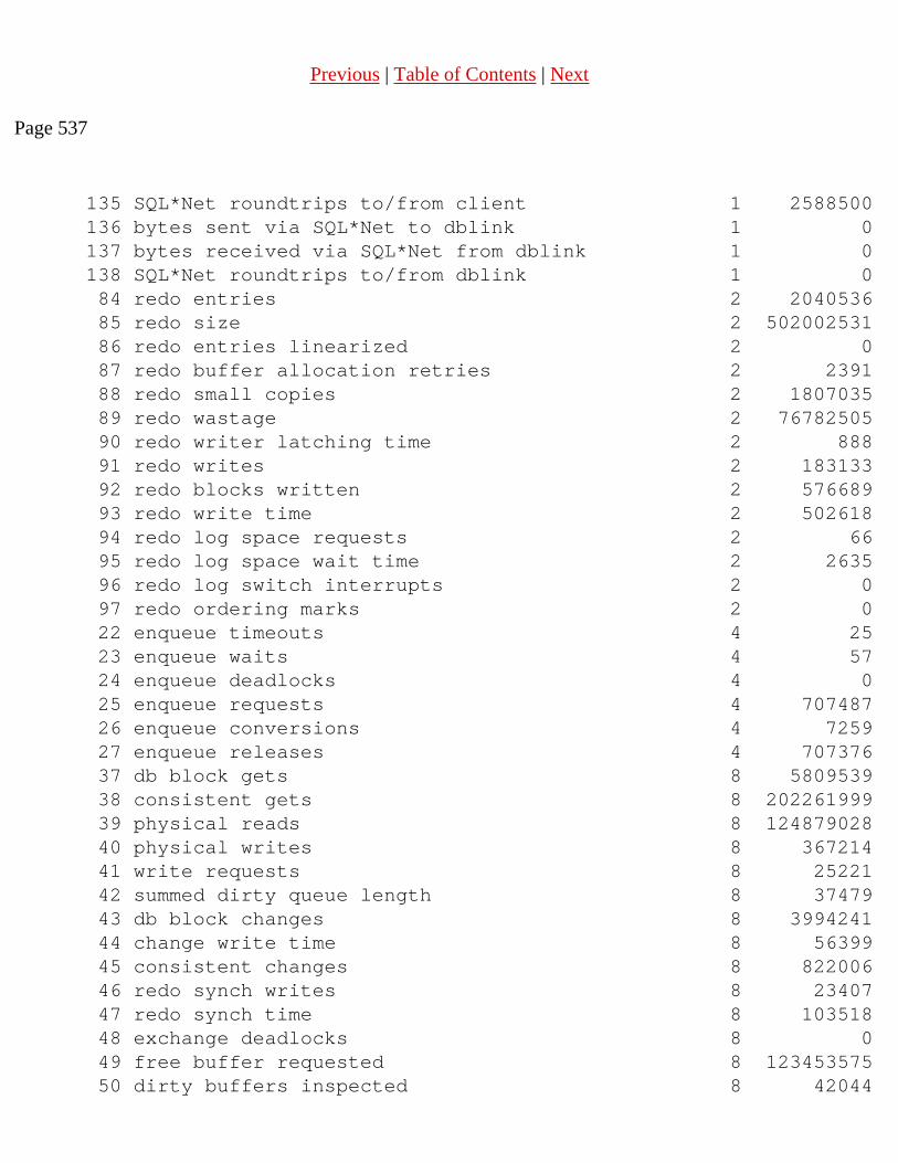
Previous | Table of Contents | Next
Page 537
135 SQL*Net roundtrips to/from client 1 2588500 136 bytes sent via SQL*Net to dblink 1 0 137 bytes received via SQL*Net from dblink 1 0 138 SQL*Net roundtrips to/from dblink 1 0 84 redo entries 2 2040536 85 redo size 2 502002531 86 redo entries linearized 2 0 87 redo buffer allocation retries 2 2391 88 redo small copies 2 1807035 89 redo wastage 2 76782505 90 redo writer latching time 2 888 91 redo writes 2 183133 92 redo blocks written 2 576689 93 redo write time 2 502618 94 redo log space requests 2 66 95 redo log space wait time 2 2635 96 redo log switch interrupts 2 0 97 redo ordering marks 2 0 22 enqueue timeouts 4 25 23 enqueue waits 4 57 24 enqueue deadlocks 4 0 25 enqueue requests 4 707487 26 enqueue conversions 4 7259 27 enqueue releases 4 707376 37 db block gets 8 5809539 38 consistent gets 8 202261999 39 physical reads 8 124879028 40 physical writes 8 367214 41 write requests 8 25221 42 summed dirty queue length 8 37479 43 db block changes 8 3994241 44 change write time 8 56399 45 consistent changes 8 822006 46 redo synch writes 8 23407 47 redo synch time 8 103518 48 exchange deadlocks 8 0 49 free buffer requested 8 123453575 50 dirty buffers inspected 8 42044

51 free buffer inspected 8 86462 52 commit cleanout failure: write disabled 8 0 53 commit cleanout failures: hot backup in 8 0 progress
54 commit cleanout failures: buffer being w 8 164 ritten
55 commit cleanout failures: callback failu 8 2769 re
56 total number commit cleanout calls 8 547911 57 commit cleanout number successfully comp 8 538392 leted
58 DBWR timeouts 8 10503 59 DBWR make free requests 8 38615
continues
Page 538
Listing 22.1 Continued
60 DBWR free buffers found 8 18186694 61 DBWR lru scans 8 42222 62 DBWR summed scan depth 8 20800400 63 DBWR buffers scanned 8 20699788 64 DBWR checkpoints 8 998 70 recovery blocks read 8 0 71 recovery array reads 8 0 72 recovery array read time 8 0 73 CR blocks created 8 125716 74 Current blocks converted for CR 8 14791 99 background checkpoints started 8 18 100 background checkpoints completed 8 18 28 global lock gets (non async) 32 1 29 global lock gets (async) 32 0 30 global lock get time 32 0 31 global lock converts (non async) 32 0 32 global lock converts (async) 32 0 33 global lock convert time 32 0 34 global lock releases (non async) 32 0

35 global lock releases (async) 32 0 36 global lock release time 32 0 78 next scns gotten without going to DLM 32 0 79 Unnecessary process cleanup for SCN batch 32 0 ing
80 calls to get snapshot scn: kcmgss 32 2619387 81 kcmgss waited for batching 32 0 82 kcmgss read scn without going to DLM 32 0 83 kcmccs called get current scn 32 0 65 DBWR cross instance writes 40 0 66 remote instance undo block writes 40 0 67 remote instance undo header writes 40 0 68 remote instance undo requests 40 0 69 cross instance CR read 40 0 98 hash latch wait gets 40 0 118 table scans (short tables) 64 366085 119 table scans (long tables) 64 10819 120 table scans (rowid ranges) 64 15 121 table scans (cache partitions) 64 0 122 table scans (direct read) 64 15 123 table scan rows gotten 64 904956876 124 table scan blocks gotten 64 129018277 125 table fetch by rowid 64 31893640 126 table fetch continued row 64 506029 127 cluster key scans 64 135034 128 cluster key scan block gets 64 363979 129 parse time cpu 64 34740 130 parse time elapsed 64 55148 131 parse count 64 532516 132 execute count 64 2390178 139 sorts (memory) 64 40412 140 sorts (disk) 64 268 141 sorts (rows) 64 49141580 142 session cursor cache hits 64 0
Page 539
143 session cursor cache count 64 0 11 CPU used when call started 128 4896911 14 process last non-idle time 128 6.2794E+11 17 messages sent 128 160593 18 messages received 128 160593

19 background timeouts 128 31883 75 calls to kcmgcs 128 90759 76 calls to kcmgrs 128 4168092 77 calls to kcmgas 128 306090 102 transaction lock foreground requests 128 0 103 transaction lock foreground wait time 128 0 104 transaction lock background gets 128 0 105 transaction lock background get time 128 0 106 transaction tables consistent reads - un 128 143669 do records applied
107 transaction tables consistent read rollb 128 131 acks
108 data blocks consistent reads - undo reco 128 678275 rds applied
109 no work - consistent read gets 128 194428691 110 cleanouts only - consistent read gets 128 25194 111 rollbacks only - consistent read gets 128 86452 112 cleanouts and rollbacks - consistent rea 128 54180 d gets
113 rollback changes - undo records applied 128 14117 114 transaction rollbacks 128 1520 115 immediate (CURRENT) block cleanout appli 128 73789 cations
116 immediate (CR) block cleanout applicatio 128 79374 ns
117 deferred (CURRENT) block cleanout applic 128 264576 ations
144 cursor authentications 128 95248
NOTE
Be careful when you use this view. Some of the statistic values in this view can get so large that, due to existing bugs in some Oracle versions, these may show wrong values.n
The statistic we are interested in is CPU used by this session having a statistic# value

of 12:
12 CPU used by this session 1 4896925SQL> select * from v$sysstat order by class,statistic# WHERE name = `CPU usedby Âthis session'
Page 540
Now the value of CPU used by this session is in hundredths of a second. Converting the value into minutes, we modify the query as follows:
col name format a35col value format 999.99 heading "Time in | Mins"select statistic#,name,class ,value/60/100 valuefrom v$sysstatwhere statistic# = 12/STATISTIC# NAME CLASS Mins---------- ---------------------------------- ----------- -------- 12 CPU used by this session 1 817.56
This output shows that the RDBMS with all its background and foreground server processes has consumed approximately 817 minutes of CPU time since startup. This is again information at an overall level. You now want to find which session has consumed how much of the CPU resource.
There is another dynamic performance view called V$SESSTAT. Basically, the only difference between the two is that V$SYSSTAT stores the summary level information, and V$SESSTAT stores information at the session level; V$SESSTAT can be called the child table of V$SYSSTAT. You can use the information in V$SESSTAT to find out which session is consuming the maximum CPU. You do that by using the script in Listing 22.2.
Listing 22.2 Script and Output to Produce CPU Usage Report
col prog format a10col value format 9999.99 heading "Time In| Mins"
Select a.sid, spid, status, substr(a.program,1,10) prog, a.terminal, osuser, value/60/100 value

From v$session a, v$process b, v$sesstat cWhere c.statistic# = 12And c.sid = a.sidAnd a.paddr = b.addrOrder by value desc;
Time In SID SPID STATUS PROG TERMINAL Schema Mins--------- -------- -------- ---------- ---------- -------- -------- 45 11145 INACTIVE C:\ARMS\BS Windows PC RICHARDH 95.87 95 12370 INACTIVE C:\WINDOWS Windows PC MATHEWS 22.99 47 9778 INACTIVE C:\ARMS\BS Windows PC KARENC 10.22 22 9295 ACTIVE C:\ARMS\DE Windows PC SUNIT 3.96 37 14427 INACTIVE C:\ARMS\CS Windows PC PETER .50 107 9454 INACTIVE sqlplus@ar ttyp2 TOM .34
Previous | Table of Contents | Next

Previous | Table of Contents | Next
Page 567
CHAPTER 23
Security Management
In this chapter
● User Authentication 568
● Database Privilege Management 572
● Monitoring Database Assets 579
● Protecting Data Integrity 582
● Hardware Security 582
● Recovering Lost Data 583
Page 568
User Authentication
Users must be identified and authenticated before they are allowed access to your database. Users will be identified by Oracle, but they can be authenticated in three different ways: database, external, or enterprise authentication.
Database Authentication
Database authentication is used when a user is created and a password is specified. This is a good approach for small user communities and when there are no additional security products available. The other types of authentication require the reserved word external to be used in place of the user password.
When a user is created, a password must be selected for the user. Applying rules on a user password is called password management, and a company should have guidelines for passwords. A strong password is one that is not easily guessed, is longer then five bytes, and is not a word found in the dictionary. If the password is in a dictionary, a computer vandal may be able to guess the password by using a "brute force attack." (A brute force attack is one in which a computer vandal uses a userid and writes a program

to try different passwords that are generated from a dictionary.) A password also should expire after a certain length of time and not be reused by the same user.
Oracle now has the capability of providing password management when using database-level authentication. This is accomplished by setting parameters on a profile and assigning that profile to a user. A profile is a database entity that will specify resource limits, and when a profile is assigned to a user, it enforces those limits on the user. A profile can be created using the Enterprise Manager or SQL*Plus. The database must have resource limits turned on in order for the profile resource limits to take affect. You do this by setting the RESOURCE_LIMIT parameter in the init.ora file to TRUE. A profile can limit the number of sessions, the CPU usage per session, the number of CPU calls, the logical reads, the logical reads per call, idle time, and connect time. The profile can prevent computer vandals from utilizing all the resources from a computer in a denial-of-service attack.
The profile can now enforce password management rules, which are options that you may elect to be used:
● Locking of a user account: When a user has multiple failed logins, the account can be locked for a specified period of time.
● Password Lifetime and Expiration: A given password will now have a specified time limit for use and then will expire and have to be changed. A grace period will be given to a user after the password expires; if the user does not change the password, the account is locked. The database/security administrator can also set the password to an expired state.
● Password History: The password history option checks each newly specified password to ensure that a password is not reused for the specified amount of time or for the specified number of password changes. The database administrator can configure the rules for password reuse with CREATE PROFILE statements.
Page 569
● Password Complexity Verification: Complexity verification checks the strength of a password to make it harder for a computer vandal to defeat it. The default password complexity verification routine requires that each password
Be a minimum of four characters in length
Not equal the userid
Include at least one alpha, one numeric, and one punctuation mark
Not match any word on an internal list of simple words, such as welcome, account,

database, user, and so on.
Differ from the previous password by at least three characters.
● Database Administrator Authentication: Database administrators require a more secure authentication scheme due to the privileged nature of their tasks (such as shutting down or starting up a database). Additional authentication can be implemented using the operating system and/or a password file.
● Operating system: If the operating system provides a way of segmenting users into groups such as UNIX or NT, Oracle will recommend DBAs be placed in a special group. This enables Oracle to have additional authentication via the group id to know that a user is DBA.
● Using a Password File to authenticate DBAs: A password file for DBAs is optional and can be set up using the ORAPWD password utility. The password file will restrict administration privilege to only the users who know the password and have been granted a special role. The roles are SYSOPER and SYSDBA:
SYSOPER permits you to perform STARTUP, SHUTDOWN, ALTER DATABASE OPEN/MOUNT, ALTER DATABASE BACKUP, ARCHIVE LOG, and RECOVER, and includes the RESTRICTED SESSION privilege.
SYSDBA contains all system privileges with ADMIN OPTION, and the SYSOPER system privilege permits CREATE DATABASE and time-based recovery.
Using ORAPWDThe ORAPWD utility is executed at the command prompt of an operating system. Use the following steps:
1. Create the password file using the ORAPWD utility
ORAPWD FILE=filename PASSWORD=password ENTRIES=max_users
where FILE= is the actual filename for the password file, PASSWORD= is the password that must be used to sign on to the database as a DBA, and ENTRIES= is the maximum number of users that can have the DBA privilege.
2. Set the REMOTE_LOGIN_PASSWORDFILE initialization parameter to a valid value. This parameter has three valid values NONE, SHARED, and EXCLUSIVE. The NONE value causes Oracle to behave as if the password file does not exist; this is the default value. The EXCLUSIVE value will do the following:
❍ Restrict the password file to one database.
❍ Allow users to be granted the roles SYSDBA and SYSOPER.
Page 570
The SHARED value will allow a password file to be used by multiple databases. However, the only users recognized by a SHARED password file are SYS and INTERNAL, and you cannot add users to a SHARED password file.
3. Users can be added to the password file by using the GRANT command to assign the database administration privilege to the appropriate user, as long as the password file is in EXCLUSIVE mode. The following are examples:
GRANT SYSDBA TO jefferson
GRANT SYSOPER TO smith
NOTE
Use the REVOKE command to remove users from the password file.n
Using SYSDBAThe privilege SYSDBA permits the user to perform the same operations as OSDBA. Likewise, the privilege SYSOPER permits the user to perform the same operations as OSOPER.
Privileged users should now be able to connect to the database by using a command similar to this:
CONNECT jefferson/[email protected] AS SYSDBA
The use of a password file does not prevent OS-authenticated users from connecting if they meet the criteria for OS authentication.
If you want to list password file members, the view V$PWFILE_USERS will show all users that have been granted SYSDBA and SYSOPER system privileges for a database.
External Authentication
External authentication relies on an operating system or network authentication service. This places control outside of Oracle for password management and user authentication, although Oracle will still identify the user. A database password is not required for this type of login. To use this option, set the parameter OS_AUTHENT_PREFIX in the database init.ora file. This will tell Oracle that any user that has the same prefix as this value is to be authenticated externally. For example, if the value is set to ops$ and you have two users, ops$jones and smith, Oracle will not require a password from ops$jones, but

will require one from smith. This parameter can be set to any prefix you like and even can be set to a null string by specifying an empty set of double quotes. The init.ora parameter REMOTE_OS_AUTHENT must be set to true (the default is false) to enable Oracle to use the username from a nonsecure connection. This keeps a potential computer vandal from masquerading as a valid user.
Network authentication is accomplished with Oracle Advanced Networking Option (ANO) and can authenticate users with the following technologies:
● Network Authentication Services(such as Kerberos and SESAME): Allow a central source for password management and can enforce single sign-on using third-party software. A user is created on each database that he or she will use and database privileges will be
Previous | Table of Contents | Next

Previous | Table of Contents | Next
Page 565
can be determined by using the sharable_memory column of the V$SQLAREA view, which contains all the SQLs in the shared pool. Every session that executes the same SQL will share the same shared SQL area.
The private SQL area is the memory area that contains data such as binding information and runtime buffers. Every session that executes a SQL statement will have its own individual private SQL area for every SQL that it executes. To summarize, for multiple sessions that are executing the same SQL statement, there will be one shared SQL area and multiple private SQL areas owned individually by each of the sessions. The private SQL area is further divided into a persistent area and the runtime area.
The area of memory in which we will be required to monitor memory usage is the Program Global Area (PGA). The PGA contains data and control information for a single process. The PGA is also referred to as the Process Global Area. The contents of the PGA vary depending on the type of connection, dedicated or multithreaded.
In both architectures, the PGA will always contain the stack space, which is the memory used to store the sessions variables, arrays, and other information.
In a dedicated server option, the PGA will store additional information related to the user's session—that is, the private SQL area and other session information is stored here. In a multi-threaded option, this information is located in the SGA.
You can monitor the PGA usage and assess the per-user memory requirement on the system. The PGA memory usage can be done by using the V$SESSTAT view. The statistic# value=20 corresponds to PGA memory usage. To monitor heavy memory users, use the script in Listing 22.23.
Listing 22.23 Finding PGA Memory Usage Using v$sesstat
col value format 99999 heading "Memory |Kb"
Select sid, value/1024 value From v$sesstat Where statistic# =20 Order By value desc
Memory
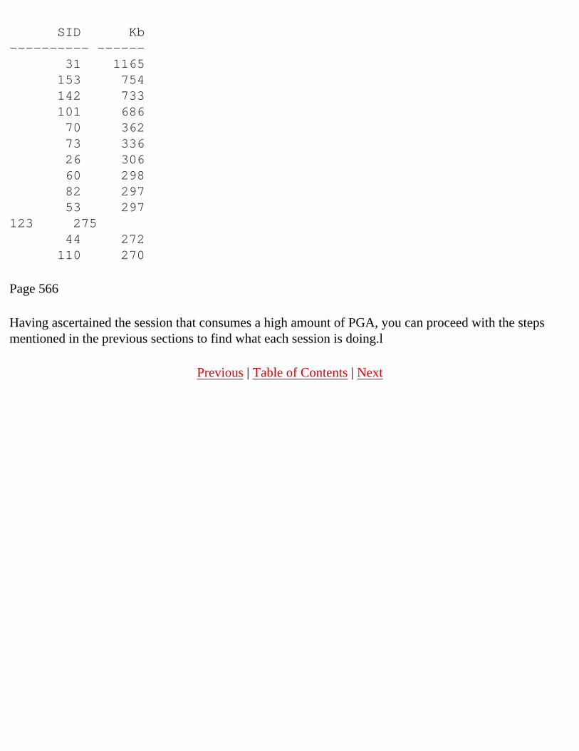
SID Kb---------- ------ 31 1165 153 754 142 733 101 686 70 362 73 336 26 306 60 298 82 297 53 297123 275 44 272 110 270
Page 566
Having ascertained the session that consumes a high amount of PGA, you can proceed with the steps mentioned in the previous sections to find what each session is doing.l
Previous | Table of Contents | Next

Previous | Table of Contents | Next
Page 563
NOTE
The SZ column refers to text plus data plus stack memory usage. This size of the text page of the Oracle executable can be determined by using the size command on the Oracle executable. After the text page size of the executable is obtained, then, theoretically, if you subtract the value obtained from the virtual memory size using the ps -ael command, you would get the actual per-process virtual memory usage of the process. But sometimes the SZ column in the ps -el command does not report the actual text page size; it reports only the page required by the process. This happens because of the demand-paging algorithm, wherein only the most required pages of text are used by the process, and the rest are brought as required from the file system.
You could use the size column report in the top command because the top command reports the total text-page size rather than the actual used-page size when it reports on the virtual memory in the SIZE column. In Listing 22.21, the size of the virtual memory used by the process ID 25623 is 8640K, which includes the complete text page.
If I try to find the size value using the ps command, the following is obtained:
$ ps -ael | grep 256,23 1 R 105 25623 25622 254 241 20 3909b001524 - ? 9:20 oracle
The ps command shows that the size of the virtual memory is 1524*4K =6096K, which is much less than the top command 8640K value because the text page size used is actually much lower than the total text page size.
Keep this in mind when computing actual memory usage of the individual processes.n
Listing 22.21 Obtaining the Virtual Memory Size by Using the top Command Output
System: arms1 Tue Sep 9 19:41:51 1997Load averages: 4.87, 4.74, 4.44211 processes: 204 sleeping, 7 runningCpu states:

CPU LOAD USER NICE SYS IDLE BLOCK SWAIT INTR SSYS0 4.98 88.1% 0.0% 11.9% 0.0% 0.0% 0.0% 0.0% 0.0%1 4.75 79.2% 0.0% 20.8% 0.0% 0.0% 0.0% 0.0% 0.0%-- ---- ----- ----- ----- ----- ----- ----- ----- -----avg 4.87 83.2% 0.0% 16.8% 0.0% 0.0% 0.0% 0.0% 0.0%
Memory: 53592K (15892K) real, 72336K (25548K) virtual, 11848K free Page# 1/20
CPU TTY PID USERNAME PRI NI SIZE RES STATE TIME %WCPU %CPU COMMAND0 ? 25623 arms 240 20 8640K 548K run 7:34 43.47 43.39 oracleor1 ? 18128 oracle 241 20 9184K 1024K run 177:07 31.29 31.23 oracleor0 ? 19523 oracle 240 20 9644K 1552K run 60:48 26.19 26.15 oracleor
Page 564
Using the output in Listing 22.22, you can determine the pid of the Oracle processes. When the pid is obtained using the SQL statements in the previous sections, the sid of the processes can be found and then further investigation can be done at the session level.
Listing 22.22 ps Command Used for finding the Memory Usage by Processes
$ ps -eal | grep oracle | sort -n -r -k 10 1 R 129 28060 28058 248 240 20 3932f00 2400 - ? 15:24 oracle 1 R 104 28049 1 246 239 20 3941080 2001 - ? 10:55 oracle 1 S 104 25751 1 0 156 20 38e1f80 1939 461b34 ? 19:02 oracle 1 S 104 15018 1 0 154 20 37c2980 1915 3d90e38 ? 198:25 oracle 1 S 104 25861 1 59 148 20 3807d00 1711 2194bac ? 32:42 oracle 1 S 104 25743 1 0 156 20 3e38380 1658 461b1c ? 23:52 oracle 1 S 104 14103 1 0 154 20 2829900 1653 3d4e338 ? 109:12 oracle 1 R 104 25739 1 255 241 20 37c2d80 1623 - ? 142:21 oracle

1 S 104 27772 1 0 156 20 372ba80 1603 461b04 ? 9:11 oracle 1 S 105 22744 22743 0 154 20 3941e80 1578 3d61da2 ? 38:59 oracle 1 S 129 25731 25727 0 154 20 335f700 1538 38c47a2 ? 0:00 oracle 1 S 104 19722 1 0 154 20 2845380 1525 3d6cb38 ? 0:05 oracle 1 S 129 28055 28053 0 154 20 3780f00 1522 3dda0a2 ? 0:00 oracle 1 S 125 25629 1 0 156 20 3738680 1511 461aa4 ? 0:01 oracle 1 S 104 7258 1 0 154 20 38e6100 1498 391e838 ? 0:00 oracle 1 S 125 25623 1 0 156 20 294f600 1493 461a8c ? 0:38 oracle 1 S 125 25621 1 0 156 20 2576080 1490 461a84 ? 1:15 oracle 1 S 125 25627 1 0 156 20 3807300 1483 461a9c ? 0:03 oracle 1 S 125 25625 1 3 156 20 3937000 1483 461a94 ? 2:00 oracle 1 S 125 25649 1 0 156 20 2958980 1478 461af4 ? 0:10 oracle 1 S 125 25647 1 0 156 20 3903b00 1478 461aec ? 0:10 oracle 1 S 125 25645 1 0 156 20 2845a80 1478 461ae4 ? 0:11 oracle 1 S 125 25643 1 0 156 20 3354400 1478 461adc ? 0:13 oracle 1 S 125 25641 1 0 156 20 391d700 1478 461ad4 ? 0:13 oracle 1 S 125 25639 1 0 156 20 3739b80 1478 461acc ? 0:13 oracle 1 S 125 25637 1 0 156 20 2852780 1478 461ac4 ? 0:14 oracle 1 S 125 25635 1 0 156 20 2888580 1478 461abc ? 0:15 oracle 1 S 125 25633 1 0 156 20 3663e80 1478 461ab4 ? 0:15 oracle 1 S 125 25631 1 0 156 20 3e40c80 1478 461aac ? 0:15 oracle 1 S 125 25619 1 0 156 20 27fb500 1477 461a7c ? 0:01

oracle
The memory usage of individual processes can also be monitored using the V$SESSTAT system view. To understand which part of memory we are looking at, we will now look into how memory is organized in the Oracle SGA. The SGA is a shared segment that comprises the shared pool, the block buffers, and the redo log buffers. The shared pool is the area in the SGA that contains constructs such as shared SQL areas and the data dictionary cache.
For every SQL that is executed on the server, there is a shared part (shared SQL area) and a private part (private SQL area). Two users executing the same SQL will use the same shared SQL area, but each user will have an individual private SQL area.
The shared SQL area contains the parse tree and the execution plan for every SQL statement. The size of the area depends on the complexity of the statement. The size of every such SQL
Previous | Table of Contents | Next

Previous | Table of Contents | Next
Page 571
assigned to that user, but the password will be the reserved word external. This will tell Oracle to identify the user only and enable an external source to authenticate the password. ANO will use an authentication server that will have usernames, passwords, and hostnames to verify the password. If the password is authenticated, the user is allowed access to the Oracle database.
● Token Devices: A token is a physical device that a user must have to establish a connection to the database. The token could be a one-time numeric password that is generated on a device the size of a thick credit card. This numeric password must be used in conjunction with a short numeric personal identification number (PIN). The Oracle server has an additional security service added to the configuration that is keeping track of the token's password. Another method is the challenge/response. A number is sent to the user (challenge) and the user enters the number on a device, which gives another number (response) that is used as the password.
● Biometric Devices: Uses a physical characteristic that is unique to the individual, currently a fingerprint scan device that can be used with ANO. The user fingerprint must first be recorded on the system, and then the user specifies the Oracle service and places his or her finger on the fingerprint reader. The finger placed on the reader will be compared with the fingerprint on the database.
Enterprise Authentication
Enterprise Authentication allows a central source for password management and can enforce single sign-on using Oracle Security Service (OSS). The user is called a global user and must be created on each database that he or she will use with the password globally. This will tell Oracle to identify the user only and enable an OSS to authenticate the password and convey user enterprise authorizations. If the password is authenticated, the user is allowed access to the Oracle database. OSS will interface with Oracle Enterprise Manager to centralize security role management and enterprise authorizations. This will enable the user to have global identities that are centrally managed.
Global RolesGlobal roles are different than database roles because they enable you to assign authorization information to (global) users across multiple databases. When a global user logs on to a database, the global roles are dynamically assigned to that user. Global roles must first be assigned to a global user in the Oracle Security Server, then have privileges associated with each global role on the database server. The privileges associated with a global role can differ between databases.
Tablespace Assignment and UsageWhen the user is created, you must tell Oracle where you want to store objects that the user creates in the database; if a storage clause does not specify where to place the objects, this is called the user's default tablespace. The default tablespace should be specified to prevent database objects such as tables or indexes from being created in the system tablespace; if the user will never have the privilege to create an object in the database, you can let it default to system. If the user will be creating

objects in the system tablespace, tablespace fragmentation or an out-of-space condition could be the result. The temporary tablespace is really a sort-work area and is used by SQL statements (such as
Page 572
ORDER BY and GROUP BY). The temporary tablespace also is used when a user builds an index. You should specify a temporary tablespace other than the system tablespace, due to the increased contention with the data dictionary.
A tablespace quota limits the size of database objects that users create in a tablespace. The default is to have no quota size limitation, but if a user has allocated database objects in a tablespace and you would like to restrict the use of that tablespace, set the quota for that user to 0 for that tablespace. With this restriction in place, the current objects in that tablespace cannot be allocated any more space, but they will remain in the tablespace.
Database Privilege Management
A privilege can be either an object privilege or system privilege. There are over 60 distinct system privileges that allow users to perform administrative activities on the database (see Table 23.1).
Table 23.1 System Privileges
Privilege Actions Allowed
ANALYZE
ANALYZE ANY Analyze any table, cluster, or index in the database.
AUDIT
AUDIT ANY Audit any schema object in the database.
AUDIT SYSTEM Enable and disable statement and privilege audit options.
CLUSTER
CREATE CLUSTER Create a cluster in own schema.
CREATE ANY CLUSTER Create a cluster in any schema. Behaves similarly to CREATE ANY TABLE.
ALTER ANY CLUSTER Alter any cluster in the database.
DROP ANY CLUSTER Drop any cluster in the database.

DATABASE
ALTER DATABASE
Alter the database; add files to the operating system via Oracle, regardless of operating system privileges.
DATABASE LINK
CREATE DATABASE LINK
Create private database links in own schema.
Page 573
Privilege Actions Allowed
INDEX
CREATE ANY INDEX Create an index in any schema on any table.
ALTER ANY INDEX Alter any index in the database.
DROP ANY INDEX Drop any index in the database.
LIBRARY
CREATE LIBRARY Create callout libraries in own schema.
CREATE ANY LIBRARY Create callout libraries in any schema
DROP LIBRARY Drop callout libraries in own schema.
DROP ANY LIBRARY Drop callout libraries in any schema.
PRIVILEGE
GRANT ANY PRIVILEGE Grant any system privilege (not object privileges).
PROCEDURE
CREATE PROCEDURE Create stored procedures, functions, and packages in own schema.

CREATE ANY PROCEDURE
Create stored procedures, functions, and packages in any schema. (Requires that user also have ALTER ANY TABLE, BACKUP ANY TABLE, DROP ANY TABLE, SELECT ANY TABLE, INSERT ANY TABLE, UPDATE ANY TABLE, DELETE ANY TABLE, or GRANT ANY TABLE privileges.)
ALTER ANY PROCEDURE Compile any stored procedure, function, or package in any schema.
DROP ANY PROCEDURE Drop any stored procedure, function, or package in any schema.
EXECUTE ANY PROCEDURE
Execute any procedure or function (standalone or packaged), or reference any public package variable in any schema.
PROFILE
CREATE PROFILE Create profiles.
ALTER PROFILE Alter any profile in the database.
DROP PROFILE Drop any profile in the database.
ALTER RESOURCE COST Set costs for resources used in all user sessions.
continues
Previous | Table of Contents | Next

Previous | Table of Contents | Next
Page 574
Table 23.1 Continued
Privilege Actions Allowed
PUBLIC DATABASE LINK
CREATE PUBLICDATABASE LINK
Create public database links.
DROP PUBLICDATABASE LINK
Drop public database links.
PUBLIC SYNONYM
CREATE PUBLIC SYNONYM Create public synonyms.
DROP PUBLIC SYNONYM Drop public synonyms.
ROLE
CREATE ROLE Create roles.
ALTER ANY ROLE Alter any role in the database.
DROP ANY ROLE Drop any role in the database.
GRANT ANY ROLE Grant any role in the database.
ROLLBACK SEGMENT
CREATE ROLLBACK SEGMENT
Create rollback segments.
ALTER ROLLBACK SEGMENT
Alter rollback segments.
DROP ROLLBACK SEGMENT Drop rollback segments.
SESSION
CREATE SESSION Connect to the database.
ALTER SESSION Issue ALTER SESSION statements.

RESTRICTED SESSION
Connect when the database has been started using STARTUP RESTRICT. (The OSOPER and OSDBA roles contain this privilege.)
SEQUENCE
CREATE SEQUENCE Create a sequence in own schema.
CREATE ANY SEQUENCE Create any sequence in any schema.
ALTER ANY SEQUENCE Alter any sequence in any schema.
DROP ANY SEQUENCE Drop any sequence in any schema.
SELECT ANY SEQUENCE Reference any sequence in any schema.
Page 575
Privilege Actions Allowed
SNAPSHOT
CREATE SNAPSHOT Create snapshots in own schema. (User must also have the CREATE TABLE privilege.)
CREATE SNAPSHOT
Create snapshots in any schema. (User must also have the CREATE ANY TABLE privilege.)
ALTER SNAPSHOT Alter any snapshot in any schema.
DROP ANY SNAPSHOT Drop any snapshot in any schema.
SYNONYM
CREATE SYNONYM Create a synonym in own schema.
CREATE ANY SYNONYM
Create any synonym in any schema.

DROP ANY SYNONYM Drop any synonym in any schema.
SYSTEM
ALTER SYSTEM Issue ALTER SYSTEM statements.
TABLE
CREATE TABLE
Create tables in own schema. Also allows grantee to create indexes (including those for integrity constraints) on table in own schema. (The grantee must have a quota for the tablespace or the UNLIMITED TABLESPACE privilege.)
CREATE ANY TABLE
Create tables in any schema. (If grantee has CREATE ANY TABLE privilege and creates a table in another user's schema, the owner must have space quota on that tablespace. The table owner need not have the CREATE [ANY] TABLE privilege.)
ALTER ANY TABLE Alter any table in any schema and compile any view in any schema.
BACKUP ANY TABLE Perform an incremental export using the Export utility of tables in any schema.
DROP ANY TABLE Drop or truncate any table in any schema.
LOCK ANY TABLE Lock any table or view in any schema.
COMMENT ANY TABLE Comment on any table, view, or column in any schema.
SELECT ANY TABLE Query any table, view, or snapshot in any schema.
INSERT ANY TABLE Insert rows into any table or view in any schema.
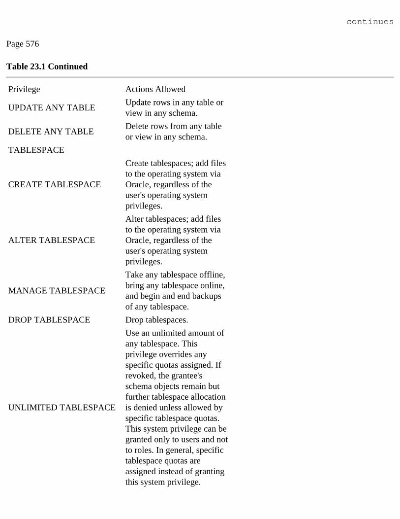
continues
Page 576
Table 23.1 Continued
Privilege Actions Allowed
UPDATE ANY TABLE Update rows in any table or view in any schema.
DELETE ANY TABLE Delete rows from any table or view in any schema.
TABLESPACE
CREATE TABLESPACE
Create tablespaces; add files to the operating system via Oracle, regardless of the user's operating system privileges.
ALTER TABLESPACE
Alter tablespaces; add files to the operating system via Oracle, regardless of the user's operating system privileges.
MANAGE TABLESPACE
Take any tablespace offline, bring any tablespace online, and begin and end backups of any tablespace.
DROP TABLESPACE Drop tablespaces.
UNLIMITED TABLESPACE
Use an unlimited amount of any tablespace. This privilege overrides any specific quotas assigned. If revoked, the grantee's schema objects remain but further tablespace allocation is denied unless allowed by specific tablespace quotas. This system privilege can be granted only to users and not to roles. In general, specific tablespace quotas are assigned instead of granting this system privilege.

TRANSACTION
FORCE TRANSACTION
Force the commit or rollback of own in-doubt distributed transaction in the local database.
FORCE ANY TRANSACTION
Force the commit or rollback of any in-doubt distributed transaction in the local database.
TRIGGER
CREATE TRIGGER Create a trigger in own schema.
CREATE ANY TRIGGER Create any trigger in any schema associated with any table in any schema.
ALTER ANY TRIGGER Enable, disable, or compile any trigger in any schema.
DROP ANY TRIGGER Drop any trigger in any schema.
Page 577
Privilege Actions Allowed
USER
CREATE ANY USER
Create users; assign quotas on any tablespace, set default and temporary tablespaces, and assign a profile as part of a CREATE USER statement.
BECOME ANY USER
Become another user. (Required by any user performing a full database import.)
ALTER USER
Alter other users in an ALTER USER statement: change any user's password or authentication method, assign tablespace quotas, set default and temporary tablespaces, assign profiles and default roles. (Not required to alter own password.)
DROP USER Drop another user.

VIEW
CREATE VIEW Create a view in own schema.
CREATE ANY VIEW
Create a view in any schema. To create a view in another user's schema, you must have CREATE ANY VIEW privileges, and the owner must have the required privileges on the objects referenced in the view.
DROP ANY VIEW Drop any view in any schema.
You should give these privileges only to users who administer the database. Object privileges allow access to and maintenance of database objects; this category of privileges is for end-users. An object privilege (see Table 32.2) can be administered directly to the user, or the privilege can be granted to a role and then the role granted to the user.
Table 23.2 Object Privileges
Object SQL Statement Allowed
ALTER ALTER object (table or sequence).
DELETE DELETE FROM object (table or view).
EXECUTE EXECUTE object (procedure or function). References to public package variables.
INDEX CREATE INDEX ON object (tables only).
INSERT INSERT INTO object (table or view).
continues
Previous | Table of Contents | Next

Previous | Table of Contents | Next
Page 585
CHAPTER 24
Backup and Recovery
In this chapter
● Backup Strategy 586
● Understanding Physical and Logical Data Loss 587
● Using Logical Backups 590
● Using Cold Physical Backups 595
● Using Hot Physical Backups 600
● Restoring from Logical Backups 604
● Using Physical Recovery 609
● Testing Strategies 618
Page 586
Backup Strategy
As most of us have learned at some point in our computing lives, data backups are an absolutely essential ingredient in most any computer system that we depend on. Disk head crashes, circuitry failure, and even catastrophic loss of data centers are all facts of life that DBAs must plan for. Fortunately, Oracle is a very robust database system with years of field-proven backup and recovery techniques that can keep your data safe when the inevitable happens. As a professional DBA, you are expected to keep your system running like a well-oiled machine. You must also take measures to ensure that the data contained in your RDBMS is safe from all sorts of threatening hazards.
Imagine that it's two weeks prior to end-of-year processing and your database system has just lost a disk drive. The CEO and CFO are both standing in your office. They want to know how long it will be before the system is back up, and they remind you that they can't lose any data from the financial system. This chapter is designed to give you the information you'll need to tell them "It won't be long" and "Of course there won't be any loss." You'll also learn some common non-emergency uses of the backup system.
It's also worth pointing out that, in this context, backups are used for data recovery both in emergency situations and in controlled situations in which you are simply moving data from one instance into another, switching machines, or just reorganizing a database.
The emphasis of this chapter will be on helping you decide, plan, and test your backup strategy. The ease with which

you'll be able to recover your database is directly related to the effort you put into your backup strategy. If you are in an uncomfortable recovery situation, you should work with Oracle support for your specific recovery needs because the details will vary on a case-by-case basis. As you design, implement, and use your backup strategy, please keep these important points in mind:
● Plan your backup and recovery strategy. Plan how you'll use your backups to recover your database.
● Test your backup and recovery strategy on a regular basis (especially important with new staff members).
● Be sure OS-level backups are still taken off the database server. Database backups do not safeguard init.ora files, Oracle installations, or operating systems.
● Perform appropriate backups of the database before and after significant modifications. This is particularly important if modifications include dropping segments or tablespaces.
● Tablespaces containing very dynamic data need to be backed up more frequently than more static tablespaces.
● Keep older backups on hand. You might not find that a table or row was deleted for months and sometimes years.
● Export your databases regularly for added protection.
● Consider distributed database backups for high-availability applications.
Page 587
Understanding Physical and Logical Data Loss
Data loss can be classified as either physical or logical. Physical data loss is the loss of components at the operating system level of a database, such as data files, control files, redo logs, and archived logs. This might be caused by a disk drive crash, someone accidentally deleting a data file, or a configuration change that overwrites any critical database file. Logical data loss is a loss of database-level components such as tables, indexes, or table records. This could be caused by someone accidentally dropping the wrong table, an application going awry, or a shortsighted WHERE clause in a DELETE statement. Not surprisingly, Oracle allows for both physical data and logical data backups. Although each backup solution could be used as a substitute for the other, you'll find out that an effective backup plan must include both to fully protect you from data loss.
The physical data backup is a copy of
● Data files
● Control files
● Applicable archived redo logs
If you lose a disk drive or need to move some of the data files around, this is the most straightforward approach to recovery. Physical backups are usually run at scheduled intervals to protect against the physical loss of a database. Indeed, if you want to ensure that you can recover the system to the last commit, you must have a physical backup as a base, as well as the archive and redo logs that have accumulated since the last physical backup.

Physical backups are further categorized into cold and hot backups. Cold backups are used when you have the option of shutting down the database long enough to back up the system. Hot backups provide a physical backup when the database is open and available for use by users. This allows an Oracle database to operate 24 hours a day, 7 days a week (24/7) and still be backed up at regular intervals. Unless you absolutely must have your database running in a 24/7 cycle, you are much better off using cold backups. As you will see, hot backups are not for the meek and must be thoroughly tested before you rely on them.
Please be aware that the term cold backup is synonymous with offline backup, as is hot backup with online backup.
Backup Frequency and ARCHIVELOG Mode
Two essential parts of planning backups are choosing the proper backup frequency for your database and deciding whether to run in ARCHIVELOG mode.
When choosing a backup interval, always ask yourself, "How much data can I afford to lose?" If your database is not running in ARCHIVELOG mode, you could lose all transactions since your last backup. If your business needs allow the database to lose one week's worth of transactions, you would need to back up the database at least once per week.
continues
Previous | Table of Contents | Next

Previous | Table of Contents | Next
Page 584
A cold backup has the virtue of having the least number of steps in the restore process, which usually means the least chance of error, and it is faster than a hot backup.
Logical Backup
A logical backup using the Oracle Export utility creates a file that has the information to re-create data structures and the data contained in the database. This information can be stored on a disk device or tape media. A logical backup takes longer than a physical backup and may require additional work in preparing the database for recovery. There are three Export modes:
● User mode, which backs up all objects owned by a user
● Table mode, which backs up specific tables owned by a user
● Full database, which backs up all objects of the database
You can control the Export utility using a parameter file to perform custom backups of data on the database. You can perform an export at three levels of data collection: incremental, cumulative, and complete. An incremental export backs up only data that has changed since the last incremental export. A cumulative export exports data only from tables that have changed since the last cumulative export; this export is used to condense the incremental exports. A complete export exports all data contained in a database. You should execute a complete export on a limited basis, due to the large volume of data collected.
Exports can be very flexible, but a regular schedule is important. It is a good idea to do a complete export on the first day of the month, an incremental export every day, and a cumulative report every weekend.l
Previous | Table of Contents | Next

Previous | Table of Contents | Next
Page 581
Statement Option
SYNONYM CREATE SYNONYM, DROP SYNONYM
SYSTEM AUDIT AUDIT, NOAUDIT
SYSTEM GRANT
GRANT system privileges/role TO user/role REVOKE system privileges/role FROM user/role
TABLE CREATE TABLE, ALTER TABLE, DROP TABLE
TABLESPACE CREATE TABLESPACE, ALTER TABLESPACE, DROP TABLESPACE
TRIGGER
CREATE TRIGGER, ALTER TRIGGER, ENABLE or DISABLE, ALTER TABLE with ENABLE, DISABLE, and DROP clauses
USER CREATE USER, ALTER USER, DROP USER
VIEW CREATE [OR REPLACE] VIEW, DROP VIEW
Auditing DML on Database Objects
You can audit a specific schema object using the following syntax:
AUDIT object_opt ON schema.objectBY SESSION/ACCESS WHENEVER NOT/SUCCESSFUL;
You can specify an object option, such as insert or update, or you can use the keyword ALL to specify all object options.
AUDIT insert,updateON scott.emp_tableWHENEVER NOT SUCCESSFUL;

AUDIT ALLON scott.emp_tableWHENEVER NOT SUCCESSFUL;
Administering Auditing
If you choose to store the audit records on the database, it is a good idea to run reports on the audit table on a daily basis and then delete the data to conserve space. The audit table should have restricted access, and all activity against the SYS.AUD$ table should be recorded by using the following statement:
AUDIT INSERT, UPDATE, DELETE, SELECTON sys.aud$BY ACCESS;
Auditing can create excessive overhead on a database, so be very selective. The BY SESSION clause in the audit statement causes Oracle to write a single record for all SQL statements of the same type that were used in the same session. The BY ACCESS clause in the audit statement causes Oracle to write one record for each audited statement. If you audit data definition language (DDL) statements, Oracle automatically uses BY ACCESS, no matter which clause is
Page 582
specified. To maintain a secure environment, you should implement a policy to decide which actions to audit.
The following AUDIT SQL statement shows how to use some of the more restrictive options:
AUDIT statement_opt/system_privileges BY user (optional) BY session/access WHENEVER NOT/SUCCESSFUL;
The next code sample shows how to audit statements relating to roles and a session:
AUDIT role;AUDIT session whenever not successful;.
Protecting Data Integrity
You can protect data integrity through the use of secure user connections and encryption algorithms. Passwords can now be encrypted when users sign on to an Oracle database. The password is encrypted

using a modified DES (data encryption standard) algorithm. Encryption is turned on by setting an environment variable on the client machine and the init.ora parameter on the database server. You must set the client machine's environment variable ORA_ENCRYPT_LOGIN to TRUE.
NOTE
This variable varies depending on the operating system. You must also set the DBLINK_ENCRYPT_LOGIN init.ora parameter to TRUE on the database server.n
Oracle will encrypt the password of a userid when a database session is initiated, but it will not encrypt the altering of the password.
Computer vandals can compromise data integrity by modifying the data or DML that travels on a network, which can result in a logical-corrupt database. When the integrity of a database is in question, it is very costly and time-consuming to restore.
Encrypting all your data is the perfect solution to potential security breeches, because if the data is being passively monitored by computer vandals they can't use the data and will probably look for easier prey. Oracle's Advanced Network Services provides this additional level of security and more. The ANO currently offers two encryption algorithms, RSA and DES, with different key lengths. For use in the U.S. and Canada, 56-bit RSA RC4, 56-bit DES, and 128-bit RSA are available; for export outside the U.S. and Canada, 40-bit RSA RC4 and 40-bit DES40 are available. Data integrity is protected by using cryptographic checksums using the MD5 algorithm. This ensures that the data is not tampered with between the time it leaves a client workstation and the time it arrives at the database server.
Hardware Security
Computer hardware needs to be stored in a restricted area where access is limited and where appropriate fire control mechanisms are in place. The electricity should be clean, meaning not
Page 583
subject to power surges or outages. Clean electricity is usually provided by an uninterrupted power supply (UPS).
Recovering Lost Data
In your security plan, you must specify how to recover data lost due to a security breach. There is a saying: "Your system is only as good as your last backup and your ability to recover." That sums up my philosophy on database recovery. Following are some good questions to ask yourself regarding backups:

● How is the backup media physically secured?
● Is the backup media shipped offsite when the backup is complete, in case of a situation in which the data center is lost?
● Is the backup media replaced in accordance with the manufacturer's guidelines?
● Is the backup hardware cleaned regularly?
● Is the backup verified as readable and available for recovery?
● Is there a backup log that shows which backup media was used for a particular day and how many times the media has been used for backup?
There are two ways to back up an Oracle database. The first is by using an operating-system backup called a physical backup; the second is by using the Oracle Export utility, which creates a logical backup.
Operating System Backup
An operating-system backup requires a utility that is specific to the operating system and that enables the DBA to restore the database by using an operating-system restore utility. You can perform the operating-system backup with the database down (a cold backup) or with it up (a hot backup). A hot backup is used in shops that require high-database availability. A hot backup enables tablespaces to be backed up while online and available for transaction processing, or while offline and unavailable. A cold backup must include all Oracle data files, control files, and online redo log files (for reference, I call these files the operating-system backup file set). A hot backup is considered a partial backup because it backs up only the files requested.
You can operate the database in ARCHIVELOG mode and in NOARCHIVELOG mode. The ARCHIVELOG mode means that as the online redo logs are filled, their contents are archived, which frees the current redo log. The archive redo logs are used to recover the transactions recorded on them or to redo them in the event of a database recovery. To perform a hot backup, the database must be in ARCHIVELOG mode. The NOARCHIVELOG mode means that online redo logs are not archived when they are full, but are written over by the latest transaction. Therefore, only the current redo logs are available for recovery. If you don't archive, you must make a backup of the operating-system file set, and when the database is restored, you must restore all the files in the operating-system backup file set.
Previous | Table of Contents | Next

Previous | Table of Contents | Next
Page 588
continuedYou can't lose any transactions in production OLTP systems. Running in ARCHIVELOG mode is highly desirable (when practical) because it allows you to fully recover your database to the last commit, even if your last physical backup was two days ago.
Even with ARCHIVELOG mode enabled, you must still make regular physical backups of the system. You must have all the archived redo logs since the last physical backup to fully recover a database. A regular physical backup will reduce the amount of space needed to store archived redo logs, as well as reduce the risk from losing transactions because of a lost or damaged archived redo log.
Physical backups should be used for recovery on the same machine, Oracle version, and instance from which they originated. Therefore, physical backups should be considered non-portable. They are usually only useful for safeguarding data on the same machine and instance against data loss.
One exception to this rule is when you want to completely transfer a database from one system to another. As long as both machines are of the same architecture, OS version, and Oracle version, you can just copy the physical components of a database from system A to system B. If any of these conditions are not met, or if you are just in doubt, use a logical backup to move your data.
A logical data backup is usually a collection of SQL statements to re-create the database objects (the database itself, tables, indexes, grants, roles, and so on), as well as the individual records in an ASCII format.
Oracle's logical backup system should be used when you need to move specific data between instances, or when you need to copy all of an instance's data between differing system archi-tectures, OS versions, or Oracle versions. Logical backups are usually run by the DBA on an as-needed basis, although there is certainly a need for somewhat regular logical backups in addition to physical backups.
In developer environments, application developers should work with DBAs to plan a logical backup strategy. Typically, two copies of the database exist: one that is production and another that is used by the developers to debug their applications. The development database should be synchronized with the production database periodically.
Let's talk about some practical real-world problems. You must have your database running in ARCHIVELOG mode and the archiver must be running for you to recover your system to the last commit. The following sections list common backup needs and the recommended backup methods. The remainder of this chapter will cover the actual mechanics of the backup and recovery methods provided by Oracle.
To help illustrate the correct usage of each backup system, the following provide several corresponding examples:
Page 589
For the cold physical backup,
● Provides protection against physical loss of the database. Allows you to shut down your database long enough for backups to be run.
● The system administrator will be upgrading your disks from 4GB each to 9GB each. You need to back up the system and restore it in the same directory structure on the new drives.
For the hot physical backup,
● Your business needs demand that the database be available 24 hours a day, 7 days a week.
● Provides protection against physical loss of the database. You are not able to shut down the database long enough for backups to run.
For the full logical backup,
● You do not have another physical system for a test bed, but you do have a production and test instance on the same machine and you want to synchronize them occasionally.
● The new server was just installed and will be replacing your old machine. Your old and new database servers are different platforms (such as Sun and HP).

For logical backup of a specific table,
● You need to move table ABC from the JSMITH schema to the TGASPER schema.
● You will be dropping table ABC, although you would like to save a backup copy of it just in case.
For logical backup of a specific user,
● You have just been told that user JSMITH can be dropped. This user owns several tables, and you think there is a chance that someone might want them later, so you want to back up just the JSMITH schema.
● There is an application using tables contained entirely in a single schema. You are planning to upgrade the application and must run a script to "update" the tables and indexes for the new version to work correctly.
TIP
These specific cases illustrate which backup methods are appropriate for the different situations you will encounter throughout your database's life. Don't rely on a single backup method. Although most DBAs understand the need for physical backups, many do not run logical backups regularly. This makes them vulnerable to an inadvertent DROP command. Remember that DROPs are immediate; there is no rollback. With help from Oracle Support, it is possible to use your physical backups to recover a dropped table. This is a very time-consuming and expensive process that probably can be avoided by having a logical backup on hand. Remember that the system does not need to be shut down for logical backups.
continues
Page 590
continued
Making a logical backup is very important to do before you run a SQL script that you have not thoroughly examined. DROPs or DELETEs might lurk unexpectedly, just waiting to zap your database!
If you run hot backups as your physical backup, you should also run cold backups when you have the opportunity. Because of the complexity of hot backups, it gives many DBAs (myself included) a warm fuzzy to know that we have a fairly recent cold backup in our back pockets. You can never have enough backups.
Using Logical Backups
Oracle provides us with logical backups through the EXP facility (IMP is used for logical recovery). You can use EXP either entirely in batch mode, entirely interactively, or interactively with some keywords specified. Before we discuss the operational aspect of EXP, let's look at the available keywords. Running exp HELP=Y will show all of them, as seen in Listing 24.1.
Listing 24.1 EXP Keywords: Output of exp HELP=Y.
oreo:/opt/oracle/bin$ exp help=y
Keyword Description (Default) Keyword Description (Default)--------------------------------------------------------------------------USERID username/password FULL export entire file (N)BUFFER size of data buffer OWNER list of owner usernamesFILE output file (EXPDAT.DMP) TABLES list of table namesCOMPRESS import into one extent (Y) RECORDLENGTH length of IO recordGRANTS export grants (Y) INCTYPE incremental export typeINDEXES export indexes (Y) RECORD track incr. export (Y)ROWS export data rows (Y) PARFILE parameter filenameCONSTRAINTS export constraints (Y) CONSISTENT cross-table consistencyLOG log file of screen output STATISTICS analyze objects (ESTIMATE)

The keywords shown in Listing 24.1 are explained below.
USERID is the user ID/password that EXP will use to log in to the database to perform the export. At the minimum, you must have the CONNECT SESSION privilege enabled to use EXP. If you intend to export another user's objects, you must have the EXP_FULL_DATABASE privilege. A DBA user, of course, can do anything.
TIP
You can use EXP with remote databases using the usual USERID/PASSWORD@REMOTE_NAME convention.
FULL specifies whether you are exporting the entire database or not. It defaults to N.
BUFFER is used to determine how many rows will be loaded into memory before committing to the export file. The default value is OS dependent. The larger your buffer, generally the faster
Previous | Table of Contents | Next

Previous | Table of Contents | Next
Page 591
your export will run (and the more system memory will be used). You can compute the number of rows that will fit into the buffer as follows:
rows=buffer_size/maximum_row_size
If the table contains a LONG column, only one row will be in the buffer at one time.
OWNER lists the schemas you want to export. Use this keyword if you are exporting full schemas. If ROWS=N, only the SQL code needed to regenerate a schema will be exported—no table rows.
FILE is the name of the export file. You should use a filename that is reasonably descriptive of the data contained. In some OSs (UNIX in particular), you can export directly to a tape device. This is particularly useful for large database backups when you don't have enough disk space anywhere for the export file.
CAUTION
When you specify a filename for the FILE keyword, be aware that these files can be rather large, depending on what you are exporting. In OSs like UNIX, you can export directly to tape, which eliminates this problem. If this is not an option, you will have to break up your export into small enough pieces to fit in either several different filesystems or in one location, so that each piece can be moved off to tape before the next piece is created in a subsequent EXP run. You may want to run EXP during off hours to reduce the impact of a full filesystem.
TABLES lists individual tables you want to export. If ROWS=N, only the SQL code needed to regenerate the specified tables is exported; no rows are exported.
COMPRESS has many implications when it is time to import the data. COMPRESS=Y will cause IMP to construct the initial extent of a new object to be large enough to hold all the object's data. For instance, if a table has four extents and each one is 20MB in size, the initial extent of the new table will be approximately 80MB. If COMPRESS=N, the new table will have four 20MB extents just as the original did.
CAUTION

Although COMPRESS=Y is very useful when you are trying to reorganize a table (to reduce the number of extents, thereby improving performance), you need to do some homework before using this option. Suppose you have a table, "ORDERS," that has these extent sizes: 30MB, 100MB, 1000MB, 1500MB, 1500MB, and 1000MB. The total size of this table is a little more than 5GB. Now suppose your machine only has disk drives of 2GB and 4GB. The largest single extent your system could have is 4GB, yet Oracle will expect to find a 5GB extent. The import process will not work because Oracle will be unable to allocate a 5GB extent. Before using COMPRESS=Y, use the following SQL statement on each table you intend to export:
SELECT SUM(BYTES) FROM DBA_EXTENTS WHERE SEGMENT_NAME=<table name>
AND OWNER=<table owner>
Using this statement will help make sure you can accommodate the table in a single extent.
Page 592
RECORDLENGTH is used for moving export files to an Oracle database on another operation system. If you are moving from system A to system B, you must know what the record size is on system B. This information is found in the operating system documentation supplied by Oracle.
GRANTS indicates to EXP whether to export GRANTS associated with objects being exported.
INCTYPE specifies a COMPLETE, CUMULATIVE, or INCREMENTAL backup. You must use a USERID with EXP_FULL_DATABASE because this option is only useful with FULL=Y. In most OLTP production environments, this capability is seldom used.
NOTE
A CUMULATIVE or INCREMENTAL export will export an entire table if it has changed. EXP will not just export changed rows. If you do choose to use this option, be sure you regularly perform a COMPLETE export to keep your baseline export current.n
INDEXES indicates if you want to export the indexes on the tables being exported.
RECORD specifies whether or not Oracle keeps track of a COMPLETE, CUMULATIVE, or INCREMENTAL export. This is useful in the following case:

You normally run a COMPLETE on Sunday and CUMULATIVEs on Monday through Friday. Tuesday night you plan to reload the test system with a COMPLETE export of the production system. If RECORD=Y when you exported the production system Tuesday night, Wednesday's CUMULATIVE export will be based on Tuesday night's COMPLETE instead of Sunday's. Basically, RECORD=N will be used if you are running an export on the database out of sequence with your normally scheduled exports.
ROWS indicates whether or not you want to export the data contained in the tables you are exporting. If ROWS=N, only the SQL code needed to re-create the table will be exported.
PARFILE is the name of a parameter file containing any valid keyword settings used for EXP. Here's an example of a parameter file:
TABLES=CUSTOMER,VEDOROWNER=SUSANCOMPRESS=NRECORD=N
As you can see, there's nothing fancy about a parameter file. It only has a keyword and value on each line. This is particularly useful if you have a standard export that you need to run periodically because you don't need to worry about forgetting to set a keyword.
CONSTRAINTS indicates whether or not you want to export constraints associated with the objects you are exporting.
CONSISTENT is useful if you are exporting tables while they are also being updated. CONSISTENT=Y ensures that each table in the export is consistent to a single point in time. If EXP encounters an updated row while exporting a table, it will use the rollback infor- mation and export the old version. If a new row is inserted, EXP will ignore it. Do not use
Page 593
CONSISTENT=Y unless it is needed because EXP will keep a rollback segment during the entire export. Because this also places extra load on your database, it is an option best used during off hours.
If you encounter a Snapshot too old error, you probably need to run your export during a period of lighter system load. You may even need to run it with the database open in RESTRICT mode to keep users from updating the database during your export. You may also need to export while in RESTRICT mode if you need a consistent view of several tables. CONSISTENT=Y provides read consistency only on a per-table basis.

LOG is a filename where you would like to save the export messages and errors. Normally, EXP just displays this information onscreen. However, because the information may race by too quickly for you to read, you'll probably want to save your EXP log output to file. All the messages and errors are shown on your screen, even when you specify a LOG filename.
TIP
If you are using a UNIX system, you can redirect EXP's screen output to /dev/null if you would rather not see the messages fly by on your monitor. If EXP is displaying a large amount of information, it will usually run faster if you redirect the output to /dev/null. This is because it is much faster for UNIX to simply throw away the information than send it to your screen.
STATISTICS specifies how statistics are generated when the exported file is imported. The options are COMPUTE, ESTIMATE, or NONE. If your export is large, setting STATISTICS to ESTIMATE or NONE will save you time (NONE saves the most). You can always use the ANALYZE TABLE command later to generate the statistical data.
DIRECT is a recent enhancement of EXP. It greatly improves exporting performance by reading the data blocks directly (rather than going through the normal database engine). Generally, if you have this option, you should use it! Your exports will run much faster.
FEEDBACK is a recent addition to EXP. If you set FEEDBACK=n (where n is some positive integer) EXP will display a period (.) for every n rows it exports. Setting FEEDBACK=0 disables this feature.
You can enter as many keywords as you want in any order on the command line. Use the following syntax:
exp [<keyword>=<value>[,<value>,...] [<keyword>=<value>[,<value>...] ...]]
Generally, I prefer to use EXP entirely in batch mode because I can easily repeat the command, either unchanged or with minor modifications. If EXP needs more information than you provided on the command line, such as the user ID/password, it will prompt you to enter it. To run EXP entirely interactively with no keywords, just type in exp at your system's command prompt. EXP will prompt you for all the information it needs.
Full Logical Backups
EXP is particularly well suited for full logical database backups. The only requirements are that you must have the EXP_FULL_DATABASE privilege and you must have enough storage space for

Previous | Table of Contents | Next

Previous | Table of Contents | Next
Page 621
CHAPTER 25
Integrity Management
In this chapter
● Introduction622 ● Implementing Locks622 ● Analyzing v$lock627 ● Monitoring Locks on the System631 ● Avoiding Locks: Possible Solutions635 ● Implementing Locks with Latches638
Page 622
Introduction
As the size of the database and the number of users on the system increases, complexity in terms of internal resource contention also increases thus leading to performance problems. The general symptoms of such internal contention are: there is enough free memory, the CPU is not very busy, but still there are performance problems on the system. Such symptoms would make a novice administrator wonder what is happening on the system. The aim of this chapter is to empower the administrator to identify such contention issues. The resources that are addressed in this chapter are locks and latches.
Implementing Locks
Locks may never be required for a single user database, but when you work in a multiuser environment, it is important to have a mechanism in place that will automatically cater to data concurrency, consistency, and integrity issues. Oracle automatically caters to these issues by acquiring different types of locks on behalf of the user to allow or prevent simultaneous access to the same resource by different users and ensuring that data integrity is not violated. Resource here means user objects such as tables and rows. While implementing locks, one of the key issues to keep in mind is that it should not be a bottleneck on the system, preventing concurrent access to data. Oracle will therefore automatically acquire locks at different levels, depending on the database operation being performed to ensure maximum concurrency. For example, when a user is reading data of a row, other users should be allowed to write to the same row. No user should be allowed to drop the table, however. These issues,
relating to which transaction should be allowed what level of access to an object or data, are implemented using the different locking levels, which we will be covering in the next section.
Need for Locking
Before we actually get into the intricacies of locking, let's examine the various scenarios under which locking becomes really important. The following are a few of the instances that explain why data consistency and concurrency are so important:
● A user is modifying data in a table, and at the same time another user is trying to drop the same table. Oracle prevents this from happening by acquiring a table-level lock for the first user. The second user, who wants to drop the table, waits for the table lock to be released by the first user, after which he or she can drop the table.
● User A is trying to read some data within a transaction, which was modified and committed by User B, after User A's transaction started. User A reads the committed data of User B. This means that the data read within the same transaction is not consistent to a point of time. Oracle ensures data read within a transaction is consistent with the point of time when the transaction started. Oracle implements transaction-level read consistency using the system change number (SCN) which is explained in a later section.
● One user modifies the data, and another user modifies the same row before the first user has committed the transaction; therefore, the changes made by the first user are lost.
Page 623
● Oracle prevents this from happening by acquiring a row-level exclusive lock on the table's row and causing the second user to wait.
● One user reads data off another user's data, which is not yet committed; that is, User A reads a row that User B is changing before User B's changes are committed.
Oracle prevents this from happening by allowing User A to read the old data, that is the data before User B modified it. Oracle does this by obtaining the data from the rollback segments.
Locking Concepts
Oracle will automatically decide—depending on the context—what lock needs to be applied for the given situation to provide maximum level of data concurrency using the lowest level of restrictiveness. Oracle has two levels of locking: share and exclusive.
Share locks are implemented with higher concurrency of data access in mind. If a shared lock is acquired, other users can share the same resource. A number of transactions can acquire a shared lock on the same resource, but this is not true in the case of exclusive locks. For example, multiple users can read the same data at the same time.

Exclusive locks prevent simultaneous sharing of the same resource. For example, if one transaction acquires an exclusive lock on a resource, no other transaction can alter or modify that resource until the time the lock is released. Here again, sharing the resource is allowed. For example, if a table is locked in exclusive mode, it will not prevent other users from selecting from the same table.
You can use the levels of locking to enable concurrent access and, at the same time, ensure data integrity. Oracle achieves this goal by applying the lowest level of restrictiveness. Oracle will automatically lock either the individual row or the entire table, depending on what is needed. Oracle uses the following general guidelines to implement the level of locking it needs to apply:
● If a user is trying to read data from a row, another user should be allowed to write to the same row.
● If a user is updating the data of a row, other users should be able to read data of the same row at the same time.
● If two users are updating the same table, they should be prevented only when they are trying to access the same row.
One of the most important functionality issues that is implemented using locking mechanisms is data consistency. Oracle ensures data consistency at two levels: statement level and transaction level.
Statement-level read consistency means any statement that starts executing will see committed data that was available just before the statement started executing. All changes, committed or uncommitted, made to data while the statement was in execution are invisible. Oracle provides statement-level read consistency by ensuring that only committed data before the SCN observed at the time when the statement started executing is available.
Previous | Table of Contents | Next

Previous | Table of Contents | Next
Page 618
4. For each changed file, set the new filenames in Oracle. The following example changes Oracle internally so that it will look in the right location for a data file. Here, you have moved the rbs1test.dbf file from the /opt/oracle/dbs1 filesystem to the /opt/oracle/dbs2 filesystem.
ALTER DATABASE RENAME FILE`/opt/oracle/dbs1/rbs1test.dbf' TO`/opt/oracle/dbs2/rbs1test.dbf';
5. Now shut down and restart the database. If it fails to start up because of a missing data file, you'll need to find out where the file went and use Oracle's RENAME facility so that Oracle finds the file it needs.
Windows EnvironmentsUnfortunately, Oracle's Recovery Manager does not gracefully handle incomplete recoveries. For this reason, the task of incomplete recovery using Oracle's Recovery Manager is a task best left to Oracle Support. Incomplete recoveries are delicate procedures, and at this point you can ill afford to take the chance that Recovery Manager will issue a SQL statement that would render your database unusable.
Testing Strategies
In this chapter, we have covered a very large amount of material related to backing up and recovering Oracle databases. Most DBAs find that every site has requirements for backup/recovery that make them unique. Because you rely so heavily on your backup and recovery solutions, you must make certain that they can truly be relied upon. An untested backup and recovery solution is worst than nothing at all—it gives you a false sense of security.
The ideal situation is that you have a completely identical machine to the one you want to protect that you can use to test backup and recovery scenarios. You should start out by cloning the production system to your test system (with the databases shut down, of course). By simulating various failures (shutting the power off to disk drives, deleting files, corrupting redo log files, and so on) and having to recover from them, you'll get invaluable hands-on experience that you can never get by reading any book or attending any seminar. If you can simulate a load on the system while performing these operations, you'll get the best possible experience along with complete reassurance that your backup/recovery solution will protect you against almost any failure.
If you, like most DBAs, don't have a complete system to use for your testing, create an instance on a machine that is most similar to the one you need to protect. It is best to pick a machine that does not

already have Oracle instances. This minimizes the chance that you'll damage a working Oracle database. Copy as much of the production database to this test instance as space permits. Simulate the filesystem/disk layout as closely as possible. Use the same backup and recovery procedures you would use on the production system while simulating failures and trying to recover from them.
Page 619
No matter how you test your backup and recovery solution, make sure that you document the exact procedures you followed. Also document where you had difficulty and what your resolution was. Anytime you experience a failure on your production system, add that scenario to your failure/recovery exercises. If it happens once, it'll probably happen again. Whenever a new DBA joins your staff, have him or her perform the same disaster and recovery exercises.l
Page 620
Previous | Table of Contents | Next

Previous | Table of Contents | Next
Page 615
ORA-01113: file 4 needs media recoveryORA-01110: data file 4: `/opt/oracle/dbs/usr1test.dbf'SVRMGR> recover database automatic;ORA-00274: Illegal recovery option AUTOMATICSVRMGR> recover automatic database;ORA-00279: Change 15185 generated at 08/24/97 21:33:21 needed for thread 1ORA-00289: Suggestion : /opt/oracle/archive/test200.arcORA-00280: Change 15185 for thread 1 is in sequence #40ORA-00278: Logfile `/opt/oracle/archive/test199.arc' no longer needed for this ryORA-00308: cannot open archived log `/opt/oracle/archive/test200.arc'ORA-07360: sfifi: stat error, unable to obtain information about file.AT&T System V/386 Error: 2: No such file or directorySpecify log: {<RET>=suggested | filename | AUTO | CANCEL}
Oracle is now waiting for you to tell it what to do next. Because your complete recovery failed, you must now begin an incomplete recovery. First, cancel the current recovery by typing CANCEL. Now shut down the database normally.
The tablespace USERS uses usrtest.dbf, which Oracle cannot completely recover because of the missing archived logs. Unfortunately, your life just got much more complicated. Now would be a good time to let the spouse know you will not be home for a while because there is no way to bring the usrtest.dbf file back to a consistent state relative to the rest of the database. Your only safe alternative (from a data consistency standpoint) is to restore all the data files from your last backup and apply archived logs through log #199. You will be losing all of the transactions that have occurred since log #199. Here are the steps you'll need to follow:
1. Restore all of the data files from your last backup.
2. Try to start the database normally.
3. When Oracle says it is in need of recovery, enter this SQL statement:
RECOVER AUTOMATIC DATABASE;
4. Oracle will stop recovering when it cannot find the archived log file you are missing.

5. Cancel the recovery by entering CANCEL.
6. Cause an incomplete recovery with this SQL statement:
RECOVER DATABASE UNTIL CANCEL;
7. Reply with CANCEL at the prompt.
8. Force the database open with this SQL statement:
ALTER DATABASE OPEN RESETLOGS;
8. Immediately shut down the database.
9. Make a cold backup.
10. Restart the database normally.
Page 616
CAUTION
Be sure to make a cold backup anytime you open the database with RESETLOGS. If you do not, any archived log files will be useless because RESETLOGS makes the current archived log files incompatible with a pre-RESETLOGS backup of the database.
Through a lot of work, you can restore the data contained in the USERS tablespace up to log #199 and logically move it into the database without losing any data in other tablespaces. Doing this may create referential integrity problems with your data. Although the specific procedures for this are beyond the scope of this book, here's the general plan:
1. Restore your last backup of the system to a test machine. You'll need to re-create redo logs manually.
2. Copy all of the archived logs through #199 to the test machine.
3. Recover the database with the RECOVER DATABASE UNTIL CANCEL command.
4. Step through all of the archived logs until you reach #199. After 199, cancel the restore.
5. Open the database with the RESETLOGS option.

6. Perform a logical backup of all of the tables in the USERS tablespace.
7. Re-create the USERS tablespace on your failed system.
8. Logically restore the tables exported in step #6 back to the instance that lost the USERS tablespace in the first place.
In a situation such as this, it is best to bring Oracle Support into the process. Their expertise will provide all of the details relevant to your particular recovery situation. If you do intend to pursue this course of action, call Oracle Support before you attempt any type of recovery—do not attempt an incomplete recovery.
Renaming and Moving Database FilesThere are many times when you need to either rename files in your database or move them from one location on the server to another. Oracle does allow you to do all of this, but there are very specific steps that should be followed. The most important of these steps is that you should do all of this type of work during off-hours. You will need to shut down the database to perform many of these operations. Be aware that dropping a redo log file, changing a control file entry, or other operations within Oracle will not physically remove or rename files in the OS. You must perform these operations manually.
Control FilesThe location of control files are kept in the appropriate init.ora/config.ora file with the control_files keyword. To move control files, complete the following steps:
1. Shut down the database.
2. Copy or move a control file to the new location.
3. Edit the appropriate init.ora or config.ora file. There is a list of control files following the control_files keyword. You may change the location or name of a control file, delete a control file from the list, or add a location to a new control file.
4. Start up the database.
Page 617
Redo LogsRedo logs must be changed from within either SQL*Plus or Server Manager. Technically, you can perform this operation while the database is up and running, but it is much easier to do when you are sure there is no activity on the system. To move or rename redo logs, complete the following steps:
1. Shut down the database.
2. Start the database in EXCLUSIVE mode. The following example shows this operation from

within Server Manager:
STARTUP EXCLUSIVE;
3. Use this SQL statement to find out the group number of the file(s) you want to change:
SELECT * FROM V$LOGFILE;
Keep a note of the group number you are working with.
4. Now determine which redo log group is active:
SELECT * FROM V$LOG;
5. The active redo log group is indicated by CURRENT, shown in the STATUS column from the query run in #4. If a file you need to move is currently in an active group, switch Oracle to the next redo log group:
ALTER SYSTEM SWITCH LOGFILE;
6. Now drop the redo log group. In the example, you're dropping the #2 log group. In your system, use the number you wrote down from step 3.
ALTER DATABASE DROP LOGFILE GROUP 2;
7. Create the redo log file group with the files in the location you want. In this example, you will re-create group #2 with two files (you should always have at least two files in each redo log group). You will use 1MB for each file. Obviously, your group number, actual filenames, and size will vary according to your site requirements.
ALTER DATABASE ADD LOGFILE GROUP 2(`/opt/oracle/dbs1/log2atest.dbf','/opt/oracle/dbs2/log2btest.dbf') size 1M;
8. Shut down the database and restart it normally.
Data Files Data files are fairly easy to move around. You'll need to use Server Manager and an OS utility to actually move or rename data files. If you are relocating files as part of a physical recovery, just place the data files where you would like them to be. Here's how to change your data file locations/names:

1. Shut down the database if it is running.
2. With an OS utility, move or rename the files to the new locations or names. Be sure to keep track of exactly where files were and where they are now.
3. Start the database in MOUNT mode. The following example shows this operation from within Server Manager:
STARTUP MOUNT;
Previous | Table of Contents | Next

Previous | Table of Contents | Next
Page 624
Transaction-level read consistency means that all data seen within the same transaction are consistent to the point of time. Oracle ensures transaction-level read consistency by using the SCN mechanism and by acquiring exclusive table and row locks when needed.
Oracle implements read consistency by using the data available in the rollback segments. When a query enters the execution stage, the current SCN is determined. As it starts reading data of data blocks, the SCN of the block is compared with the observed SCN. If the block's SCN has a value greater than SCN at the start of the query, then it means that the data in those blocks have changed after the query has started executing. If this data is read from the data blocks, it is not consistent with the point in time the query started. Oracle uses the rollback segments to reconstruct the data, as rollback segments will always contain the old data—except in cases of high update activity on the system where the old data in the rollback segments could potentially be overwritten.
Locking TypesOracle automatically acquires different types of locking, depending on the operation and the resource on which it has to acquire the lock.
There are three classes of Oracle locks:
Data locks (DML locks) are acquired on tables and are used to protect data, or rather ensure integrity of data.
Dictionary locks (DDL locks) are used to protect the structure of objects—for example, the structural definition of tables and view indexes. A dictionary lock is automatically acquired by Oracle on behalf of any DDL transaction requiring it.
Internal locks and latches protect internal database structures. Latches are discussed in greater detail in the next section.
Distributed locks and Parallel Cache Management (PCM) locks are used in Parallel Server.
Only data locks and internal locks are covered in this chapter because they are more relevant in the day-to-day issues of the database.
Data LocksTable Locks (TM): Table Locks are acquired when a transaction issues the statements in Table 25.1. Table Locks are acquired by Oracle on behalf of the transaction to reserve DML access on the table and to prevent conflicting DDL operations on the table. For example, if a transaction has a Table Lock on a table, then it will prevent any other transaction from acquiring an exclusive DDL lock on the table, which is required to drop or alter the table.
Table 25.1Statements and Table Locks Acquired
Statement Type Mode
INSERT TM Row Exclusive(3) (RX)
UPDATE TM Row Exclusive(3) (RX)

DELETE TM Row Exclusive(3) (RX)
SELECT FOR UPDATE TM Row Share(2) (RS)
LOCK TABLE TM Exclusive(6) (X)
Page 625
Table 25.1 shows the different modes in which Table Locks (TM)are acquired by the RDBMS when specific statements are issued. The Type column has a value such as TM, and the Mode column has a value of 2, 3, or 6. The value TM indicates a Table Lock; the value 2 indicates a row share (RS) lock, 3 indicates a row exclusive (RX) lock, and 6 indicates an exclusive (X) lock. The value TM(3), for example, is the value that would be stored in the v$lock table, against the session that issued the statement, when the corresponding statement is issued, so you need to be familiar with these values. v$lock is the table where Oracle lists the locks currently held by the Oracle server, which is discussed in detail with examples in the section "Analyzing v$lock."
For example, when an Insert statement is issued, the Type column in v$lock will have value TM for the session and the Mode column will have value 3 which means row exclusive (RX) lock. For additional details, refer to the section "Analyzing v$lock." For all statements except the Lock table, there will be two entries in the v$lock table: one corresponding to the Table Lock (TM) and another entry corresponding to the Transaction Lock (TX). For statements such as insert update, deleting a TM lock is acquired only to prevent conflicting DDL operations on the locked objects, which means that when a user is inserting into a table, he or she acquires a TM lock in mode 3 (RX). If another user is trying to drop the same table, it will have to acquire a TM lock in mode 6 (Exclusive). The TM(3)(RX) lock will prevent the TM(6)(X) session from acquiring the lock and the second session will remain waiting. Table 25.2 illustrates lock modes acquired by a session and lock modes permitted.
Table 25.2Locking Modes and Operations Permitted
SQL Statement Table Lock Mode
Permitted Lock Modes
Select * from tname…
none RS, RX, S, SRX, X
Insert Into tname… RX RS, RX
Update tname… RX RS*, RX*
Delete From tname RX RS*, RX*
Select…From tnameFor Update Of…
RS RS*RX*S*, SRX*
Lock Table InROW SHARE MODE
RS RS, RX, S, SRX
Lock Table InROW EXCLUSIVEMODE
RX RS, RX
Lock Table InSHARE MODE
S RS, S
Lock Table InSHARE ROWEXCLUSIVE MODE
SRX RS

continues
Page 626
Table 25.2Continued
SQL Statement Table Lock Mode
Permitted Lock Modes
Lock Table InEXCLUSIVE MODE
X None
RS: Row Share SRX: Share Row Exclusive
RX: Row Exclusive X: Exclusive
S: Share
* If another transaction has already acquired a lock on the row, a wait will occur.
Transaction Locks (TX): This type of lock is acquired when a transaction issues the statements in Table 25.3. Transaction Locks are always acquired at the row level. TX Locks exclusively lock the rows and prevent other transactions from modifying the row until the transaction holding the lock rolls back or commits the data.
Table 25.3Statements
Statement Type Mode
INSERT TX Exclusive(6) (X)
UPDATE TX Exclusive(6) (X)
DELETE TX Exclusive(6) (X)
SELECT FOR UPDATE TX Exclusive(6) (X)
For TX locks to be acquired, the transaction must first acquire a TM lock on the table. For example, when an Insert statement is issued (refer to Table 25.1), a TM lock in mode 3(RX) has to be acquired. After the TM lock in RX mode is acquired, the transaction will have to acquire a TX in exclusive (X) mode (refer to Table 25.3). The TX lock will be prevented from being acquired only if another transaction has a TX lock on the same row, and the TM lock will be prevented if there is already a TM lock in exclusive (X) Mode on the table.
The other modes are 4 (Share Mode) and 5 (Share Row Exclusive), but these locking modes do not occur commonly on the database and hence do not merit much discussion.
The Share Mode (4) lock is acquired when a user issues the following statement:
Lock table <table name> in SHARE mode;

and the Share Row Exclusive lock is acquired when a user issues
Lock table <table name> in SHARE ROW EXCLUSIVE MODE;
Very few applications actually have to use these statements; therefore, they are not considered really important when compared to other day-to-day, more frequently occurring locking types.
Previous | Table of Contents | Next

Previous | Table of Contents | Next
Page 627
Analyzing v$lock
Oracle stores all information relating to locks in the database in the dynamic status table v$lock . This section analyzes various scenarios in the database when resources are locked and examines the v$lock table to see how Oracle reports the lock.
The following is a description of the structure of v$lock:
ADDR RAW(4)
KADDR RAW(4)
SID NUMBER
TYPE VARCHAR2(2)
ID1 NUMBER
ID2 NUMBER
LMODE NUMBER
REQUEST NUMBER
CTIME NUMBER
BLOCK NUMBER
The important columns of interest, which would be of use when analyzing locking situations, are as follows:
sidThis is the session identifier.
TypeThis is the type of lock acquired or waiting by the session. Example values are

TX Transaction
TM DML or Table Lock
MR Media Recovery
ST Disk Space Transaction
As said previously, this chapter covers only TX and TM locks.
lmode/requestThis column contains the mode of the lock. The possible values are:
0 None
1 Null
2 Row Share (RS)
3 Row Exclusive (RX)
4 Share (S)
5 Share Row Exclusive (SRX)
6 Exclusive (X)
If the column lmode contains a value other than 0 or 1, it indicates that the process has acquired a lock. If the request column contains a value other than 0 or 1, it indicates that the process is waiting for a lock. If lmode contains a value 0, it indicates that the process is waiting to acquire a lock.
The following select is a quick way to check whether there are any sessions waiting to acquire locks on any table.
Select count(*) From v$lock where lmode = 0
Page 628
If the select returns a value that is greater than zero, there are locks sessions on the systems currently waiting to acquire locks.

id1Depending on the type of lock, the value in this column can have different meanings. If the type of lock is TM, the value in this column is the ID of the object that is to be locked or waiting to be locked, depending on the context. If the type of lock is TX, the value in this column is the decimal representation of rollback segment number.
id2If the type of lock is TM, the value in this column is zero. If the type of the lock is TX, it is the representation of the wrap number, that is, the number of times the rollback slot has been reused.
Using this information, you can now examine various scenarios and analyze the values stored in this table in different cases. The next section covers detailed case analyses of commonly occurring locks on the database and how to read this information from v$lock view.
Case 1: A Table Locked Exclusively
For purposes of discussion, let's assume that the table that is going to be locked is the employee table and the session id is 28. Assume that one user issues the following statement:
Lock table employee in exclusive mode;
This statement will lock the table in exclusive mode. If a table is locked exclusively by a user, the only SQL statement that can be used on the table by another user is the select statement. Insert, update, delete or any DDL operation on this table by the other user's will not be permitted until the lock is released.
For examining the records in the v$lock table, use the following select:
Select sid, type, lmode, request, id1, id2From v$lockwhere sid = 28;
When you execute the select, you get the following output:
SID TY LMODE REQUEST ID1 ID2

---------- -- ---------- ---------- ---------- ----------
28 TM 6 0 7590 0
The following are the observations:
● There is only one entry in the v$lock. ● The lock acquired is a TM (Table) Lock. ● The lmode column contains the value 6, which indicates that a table-level exclusive lock has been
acquired by the session.
Page 629
● The id1 column contains the value 7590, which is the object id of the employee table. The id2 column, as expected for TM locks, has a value of 0. To obtain the description of the object, you can use the sys.obj$ table. You can use the following select:
Select name
From sys.obj$
where obj# = 7590;
Name
--------
Employee
● The request column contains the value 0, which indicates that the lock has been acquired by this session.
Case 2: Session Updating a Row of an Exclusively Locked Table
In Case 2, the table is locked exclusively by a session, and another session is trying to update a row of the same table. Here is the SQL issued by the session trying to update the table:

Update employeeSet Name = `TOM'where emp_id = `1086';
In this case, the entry for the first session in v$lock remains the same as in Case 1, but the entries for session two are very interesting. Let us assume the session id of the second session is 29. Now if you execute the following select:
Select sid,
type, lmode, request, id1,
id2From v$lockwhere sid in (28,29);
this is the output:
SID TY LMODE REQUEST ID1 ID2
---------- -- ---------- ---------- ---------- ----------
28 TM 6 0 7590 0
29 TM 0 3 7590 0
The following are the observations in this case:
● The entry for session 28 remains the same as in Case 1. ● There is one entry for session 29. This entry is for a TM lock. Note the value of lmode is 0, and
the value of request is 3. This means that session 29 is waiting to acquire a Table Lock on the table. A Table Lock has to be first acquired by session 29 to flag that it is currently using this table. This will prevent any other sessions from issuing any DDL statements on this table. This

Table Lock is basically acquired to flag or mark the table, as used by the session. The id1 column here again indicates the object id of the table, which has to be locked.
Previous | Table of Contents | Next

Previous | Table of Contents | Next
Page 649
CHAPTER 26
Parallel Query Management
In this chapter
● Introduction650 ● SQL Operations That Can Be Parallelized653 ● Understanding the Degree of Parallelism654 ● Understanding the Query Server Processes656 ● Analyzing Objects to Update Statistics656 ● Understanding the 9,3,1 Algorithm657 ● Understanding Parallel DML657 ● Parallel Execution in OPS Environment658 ● Tuning Parallel Query659
Page 650
Introduction
Large systems with significant memory and CPU resources were available for decades. However, these systems were available only with proprietary operating systems and were not very cost effective. Multiple CPU machines with UNIX open system architecture were available in the early '90s. These machines had significant hardware resources and were comparatively cheap. Oracle introduced Parallel Query Option in Oracle version 7.1 to effectively use the hardware resources available in these systems. Oracle Parallel Query Option allows long running SQL operations, mainly queries, to be spread among multiple CPUs in a coordinated fashion. This reduces the elapse time for execution of resource-intensive SQL operations.
The Parallel Query Option allows certain operations to be performed in parallel by multiple server processes. One process, known as the query coordinator, dispatches the execution of a statement to several servers, coordinates the results from all the servers, and sends the results back to the user.
Although the feature is generally referred to as PQO, it also includes:
● Parallel Load

● Parallel Recovery ● Parallel Replication ● Parallel SQL
Parallel Load
The SQL*Loader direct path allows you to load data into the same table or partition simultaneously, using multiple SQL*Loader sessions. For example:
sqlload saledba/saledba control=sales1.ctl parallel=TRUE direct=TRUE
sqlload saledba/saledba control=sales2.ctl parallel=TRUE direct=TRUE
sqlload saledba/saledba control=sales3.ctl parallel=TRUE direct=TRUE
Note the use of keywords parallel and direct in the command line. Also note the use of three different input data files for each of the sessions. Other important features of parallel load are:
● Each SQL*Loader session loads data into a separate new extent. To optimize the I/O throughput of the system, it is highly recommended to control the location and size of the new extent by using the FILE and STORAGE keywords of the OPTIONS clause. A FILE keyword can be specified in the command line or in the control file. However, a storage clause can only be specified in the control file.
● Parallel load requires that there be no local or global indexes. If any are present, it gives an error message and aborts the load. You need to manually drop the index before the load and rebuild the index once the load is completed.
● Each loading session acquires a shared lock on the table. However, each loading session is independent, and there is no communication between these sessions.
Page 651
● When a session finishes loading, Oracle joins the loaded extent(s) with the existing extents. The unused blocks from the last loaded extent are returned as free extent. This results in nonstandard sizes of the extents after the load. Truncating takes place even if you specify the extent size through a storage clause via options in the loader control file.
As mentioned above, each parallel load session loads data into new extent(s) and does not use any existing extents, even if they do not contain any data. Thus, the initial extent of a table that is loaded only by parallel loads is never used. To optimize disk space usage, you should either create a very small initial extent or put data into the initial extent by loading it without the parallel option.
Parallel Recovery

Oracle's basic read-write unit is a data block. Whenever changes are made to a block, Oracle records these changes in the form of a redo log so that the block can be reconstructed using these logs if needed. Due to media failure or for any other reason, if the contents of the present data file(s) are lost, the file is restored from a suitable backup copy and then recovery is done. The recovery process involves:
● Reading the log file and obtaining the series of changes made to the data blocks. ● Determining which data blocks need the changes to be applied. ● Reading these data blocks in the buffer cache. ● Applying the desired changes to these data blocks, from the redo log. ● Writing the modified block back to the disk.
To perform recovery in parallel you should set the initialization parameter RECOVERY_ PARALLELISM. Alternatively, you can use the PARALLEL clause of the RECOVER command. During parallel recovery, the Server Manager or SQLDBA session reads the redo log file and passes on the changes to the parallel server processes. These processes then read the corresponding data file(s) and apply the changes.
Parallel Propagation (Replication)
Replication allows you to maintain multiple images of one or more database objects in multiple databases. Oracle Server transfers data over database links between these databases to propagate changes made to the replicated objects. The SNP background processes perform the data replication. However, if the data volume to be replicated is significantly large, it might take longer to synchronize the objects. Oracle8 allows parallel replication, whereas multiple parallel server processes can be used to propagate transactions.
Parallel SQL Execution
An Oracle database is a collection of physical data files that are manipulated through various processes. A set of such background processes and a shared memory segment, collectively called Oracle Instance, enable concurrent users to interface with the database. When a user wants to use (select, insert, update, delete) the data in the database, he or she needs to connect
Page 652
to the database. On most of the UNIX systems, Oracle uses a two-task architecture. In this scheme, when a user connects to the database, an additional process (frequently known as the shadow process) is forked. The shadow process accesses the shared memory segment and the datafiles on behalf of the user.
NOTE

In a multi-threaded server (MTS) environment, when a user logs on to the database, a shared server process is used instead of the shadow process. During Parallel Query Option this shared server process acts as the query coordinator.n
Oracle stores the data in the data files in blocks. A data block is Oracle's basic data input/output unit. When the user uses data, the corresponding data block is read by the shadow process in Oracle's buffer cache (part of the shared memory segment). The block in the buffer cache can then be modified by the user shadow process. Modified data blocks (dirty buffers) are written back to the disk by the DBWR. Thus, a shadow process does the major part of the work required by the user. Operations like parsing the SQL statement, sorting the data, and so on are also done by the shadow process.
This works very well in an OLTP system where the amount of data manipulated by a user is relatively small. However, in a DSS environment, when a user generally processes huge amounts of data, the shadow process might take a while to do the required work. While the shadow process is working long and hard to manipulate the data, it is quite possible that the system has idle CPU memory resources. This is where Oracle's Parallel Query Option comes in handy. With this option, Oracle can divide a user's large data processing request into multiple, comparatively small units of work that are then concurrently executed by different processes. It uses a set of dedicated background processes, known as parallel query slaves (servers), to do such work. The shadow process gets promoted to a management role and is called the query coordinator. It is the responsibility of the query coordinator to:
1. Break down the functions into parallel pieces. 2. Ensure that a sufficient number of parallel query slaves are available. 3. Initialize the server process for the given work and assign the work among the PQO server
processes. 4. Gather the output from the slave processes and return the output. 5. Once the desired work is finished, free the query servers, making them available for other work.
Under favorable conditions, parallel execution reduces the execution time by as many factors as the number of query slaves it uses. However, it does not reduce the total CPU time taken by the SQL statement. Parallel execution uses more memory than serial execution, so if the machine does not have spare CPU and memory resources, it may not yield desired scalability.
Previous | Table of Contents | Next

Previous | Table of Contents | Next
Page 646
By using bind variables, both the previous selects in the first case can share the same select, which is stored in the library cache, thus reducing unnecessary parsing and reducing load on the latch. Using bind variables prevents multiple copies of the same select from being formed in the shared pool.
Parsing can be reduced in the shared pool or by pinning frequently used objects such as procedures and packages. The advantage of pinning these objects is that these will never be flushed out of the shared pool and subsequently the parse time is reduced. Objects that are used very frequently can be identified by the following query:
Select name ,executions
From v$db_object_cache
Where executions > <threshold limit>;
order by 2 desc;
These high-execution objects can be pinned in the shared pool using dbms_share_pool.keep(`object_name','P');.
To check the objects in the shared pool that are not pinned, execute the following query:
Select name,type,kept,sharable_memFrom v$db_object_cacheWhere kept = `NO'Order by sharable_mem desc;
Fragmentation of the shared pool can also cause high demand for these latches. A fragmented shared pool means the net free memory available in the shared pool may be large, but the total contiguous memory available may not be the same. Therefore, when an object like a large PL/SQL object with a very high memory requirement is to be located in the shared pool, it will cause a lot of smaller chunks of allocated memory areas to be flushed. These would then have to be parsed again when a user makes the request for the same SQL again. The primary cause of fragmentation is large PL/SQL objects. Fragmentation can be avoided by increasing sharing among SQL statements by use of bind variables and pinning of large PL/SQL objects using the techniques mentioned previously. l

Page 647
PART VII
Parallel and Distributed Environments
26. Parallel Query Management 27. Parallel Server Management 28. Distributed Database Management
Page 648
Previous | Table of Contents | Next

Previous | Table of Contents | Next
Page 643
11 cache buffers chains 12 cache buffer handles 13 multiblock read objects 14 cache protection latch 15 cache buffers lru chain 16 system commit number 17 archive control 18 redo allocation 19 redo copy 20 KCL freelist latch 21 KCL name table latch 22 instance latch 23 lock element parent latch 24 loader state object freelist 25 dml lock allocation 26 list of block allocation 27 transaction allocation 28 sort extent pool 29 undo global data 30 ktm global data 31 sequence cache 32 row cache objects 33 cost function 34 user lock 35 global tx free list 36 global transaction 37 global tx hash mapping 38 shared pool 39 library cache 40 library cache load lock 41 virtual circuit buffers 42 virtual circuit queues 43 virtual circuits 44 NLS data objects 45 query server process 46 query server freelists 47 error message lists

48 process queue 49 process queue reference 50 parallel query stats 51 parallel query alloc buffer 52 device information
cache buffers lru (Least Recently Used) chainThe cache buffers lru chain latch is responsible for protecting the access paths to db block buffers in the buffer cache. The buffer cache size defined by the init.ora parameter db_block_buffers resides in the SGA and contains the cached copy of data read from data files. When processes need to read data, the presence of the data in this buffer as a result of the data being read in by some process makes the read very I/O-efficient.
The buffer cache is organized in two lists: the dirty list and the LRU list. The dirty list contains the buffers, that have been modified but not written to the disk yet. The LRU list is comprised of the pinned buffers, the dirty buffers that have not yet been moved to the dirty list, and the free buffers. The pinned buffers are buffers that are currently accessed by other processes.
Page 644
The dirty buffers contain buffers that are to be written to the disk, and they then subsequently get moved to the dirty list. The free buffers are the buffers that are available for use.
When a process needs to read data from the disk that is not already present in the cache, it needs a free buffer to read in the new data. It scans the LRU list to check for free buffers. If there are excessive requests for free buffers in the buffer cache there will be a high access to the LRU list causing contention for the cache buffer LRU chain.
The contention for this latch can be minimized by the init.ora parameter db_block_lru_latches, which is available in Oracle 7.3. By increasing the db_block_lru_latches value, the contention can be minimized for this latch. The maximum value for this parameter is double the number of CPUs.
The basic reason for contention for this latch is a high request for free buffers. You can optimize the SQL statements to minimize the high demand for free buffers or increase the db_block_buffer parameter to increase the number of free buffers available on the system.
NOTE
Note that the SGA must fit into a contiguous chunk of real memory, so if the buffer cache is enlarged, you must ensure that there is enough contiguous memory available on the system to service the increase.n

redo allocation and redo copyThe redo allocation and redo copy latches control the write access to the redo log buffer. When a process requires writing to the redo log buffer, one of these latches is to be acquired by the process. If the size of the redo log information written to the redo log buffer is less than log_small_entry_max_size parameter, the process will use the redo allocation latch. If the size is greater than this value, the process is copied using the redo copy latch.
A quick way to check whether there is any contention on the redo log buffer is to check whether there are any waits associated with writing to the redo log buffer. This can be done by using the system view v$sysstat:
Select name, valueFrom v$sysstatWhere name = `redo log space requests';
Output Table:
Name Value
---------------------------------------- ----
redo log space requests 12
The size of the redo log buffer will have to be increased if the number of waits is too high.
Contention for redo allocation LatchThe contention for redo allocation can be reduced on a multi-CPU system by forcing the process to use the redo copy latch instead. Because there can be multiple redo copy latches, the copy will be done more efficiently. The number of redo copy latches is defined by the init.ora parameter log_simultaneous_copies. The maximum number available latches on the system is double the number of CPUs. For a
Page 645
single CPU system, this value is 0, and the redo allocation latch will be used. So, if there is a contention for the redo allocation latch, the value of log_small_entry_max_size can be decreased from its current value so that the redo copy latch is used.
Contention for the redo copy LatchIf the system is facing contention for the redo copy latch, it can be decreased by either increasing the value of log_small_entry_max_size (so that the redo allocation latch is used) or increasing the value of log_simultaneous_copies (so that it increases the number of redo copy latches available).
The init.ora parameter log_entry_prebuild_threshold can be increased so that the data that is written to

the redo log buffer is grouped and written out. By increasing the parameter, a number of write operations can be grouped so that they can be written out in one operation, thereby reducing requests for these latches and thus contention.
library cacheThis latch is primarily concerned with control of access to the library cache. The library cache includes shared SQL area, private sql areas, PL/SQL procedures packages, and other control structures. Shared SQL area contains SQLs that are shared among multiple sessions. By increasing the sharing of these SQLs, contention to this latch can be avoided.
Contention for this latch occurs when there is a lot of demand for space in the library cache. Very high parsing on the system and heavy demand to open a new cursor because of low sharing among processes are some of the common causes for contention for this latch.
Contention for this latch can be avoiding by using code that can be shared by multiple sessions. For example, the RDBMS treats the following two SQLs differently:
select name from employee where emp_id = 100;
and
Select name from employee where emp_id = 100;
Though both the SQL statements look the same, the hash values of these statements are different. One of the statements has select in upper case and the other one has select in lower case. Therefore, when this statement is issued, the RDBMS will parse both the statements individually as different statements, thus causing load on the latches. This situation can be avoided by developing coding standards wherein indentation and case standards are implemented so that every SQL statement written would have the same hash value as far as possible. Note that even putting more empty spaces causes one select to be different from another, causing increased parsing.
Using bind variables in SQL statements can increase the sharing of the same clauses. For example, consider the two cases, not using bind variables:
Select sal from employee where emp_id = 100;
Select sal from employee where emp_id = 200;
or, using bind variables:
Select sal from employee where emp_id := emp_id;

Previous | Table of Contents | Next

Previous | Table of Contents | Next
Page 653
SQL Operations That Can Be Parallelized
When an SQL statement is submitted, it is first parsed and then executed. After parsing and before execution, the optimizer builds the execution plan. The query coordinator process examines the operations in the execution plan to determine whether the individual operations can be parallelized.
Prior to version 8, Oracle could parallelize only SQL statements having queries or DDL operations like create index, create table, as select, and so on, whose execution plan involved a full scan of an existing table. In version 8, Oracle introduced parallel execution for insert, update, and delete operations.
Oracle8 Server Concepts Manual mentions that Oracle8 allows the following operations to be parallelized:
● table scan ● nested loop join ● sort merger join ● hash join ● "not in" ● group by ● select distinct ● union and union all ● aggregation ● PL/SQL functions called from SQL ● order by ● create table as select ● create index ● rebuild index ● move partition ● split partition ● update ● delete ● insert…select ● enable constraint (the table scan is parallelized) ● star transformation
As a rule of thumb, one can say that Oracle can parallelize any operation that involves a full table (partition) scan. Consider the following SQL statement:

select cust_id, sales_amt from sales_97 order by sales_amt;
Page 654
The execution plan consists of a full-table scan of the sales_97 table, assuming there is no index on these columns, followed by a sort on the sales_amt column. As shown in Figure 26.1, the scan and sort operations are divided and given to multiple processes. Both scan and sort are done simultaneously by different processes. Thus, PQO not only allows an operation to be done by multiple processes, but also enables multiple operations in the same SQL statement to be executed simultaneously rather than one after another. It is possible because of the creator and consumer nature of these operations. In the example, the rows fetched by the table scan operation are given to a sort operation without waiting for the scan to finish.
FIG. 26.1Parallel execution involving a full-table scan followed by a sort.
Dividing an SQL operation among multiple server processes is generally referred to as intra-operation parallelism, whereas executing multiple operations simultaneously is known as inter-operation parallelism. In the previous example, scanning and sorting operations have their own server processes. Thus, inter-operation parallelism assigns different sets of servers to each operation. Oracle can execute two operations simultaneously, in parallel, for an SQL statement. If the SQL statement has three or more operations that can be parallelized, the third operation waits until the first one finishes. The query slaves used by the first operation are then recycled and used by the third operation.
Understanding the Degree of Parallelism
The number of parallel query slaves an SQL operation can use is called the degree of parallelism. Oracle determines the degree of parallelism by considering various user inputs, instance initialization parameters, number of files, number of CPU in the system, and so on.
Determining the Degree of Parallelism
Degree of parallelism is decided from the following, in the given order:
1. 1. At SQL statement level: An SQL statement can specify the degree of parallelism through the use of parallel hint, as shown below :
select /*+ PARALLEL (sales_97, 3) */
cust_id, sales_amt from sales_97 order by sales_amt;
1. In this example, Oracle uses three query slaves to perform the full table scan operation. The sort operation requires another three slaves. Thus the SQL statement uses seven processes—six parallel query slaves and one shadow process—in all.
Page 655
2. At object level: You set the degree of parallelism associated with a table, cluster, partition, and so on through the corresponding create and alter commands. You can query the degree of parallelism of an existing object from the data dictionary from the USER_TABLES view's degree column.
Alter table sales_97 parallel(degree,3);
select degree from user_tables where table_name='SALES_97';
The first statement will set the degree of parallelism for the table sales_97 to three. Second SQL statement queries the degree of parallelism for the sales_97 table. If multiple tables are involved in an SQL operation and each of them has a different degree of parallelism, the highest degree of parallelism becomes the degree of parallelism for that SQL operation. In the following example, the SQL operation will be performed with a parallel degree of 5:
alter table sales_97 parallel (degree 3);alter table warehouse parallel (degree 5);select /*+ parallel(s) parallel(w) */w.location, s.sales_date, s.sales_valuefrom warehouse w, sales_97 swhere c.w_id = s.w_idorder by s.sales_value, w.location ;
3. Instance level: If Oracle fails to get the degree of parallelism in the previous two steps (that is, if the degree of parallelism is not specified by the user), it uses the default degree of parallelism. The process of determining the default degree of parallelism has changed with version 7.3.
In version 7.3 and later, Oracle uses the number of available CPUs and the number of disks (files, if it cannot determine the disk affinity) to determine the default degree of parallelism as follows:
Default degree of parallelism = Min (#CPU in the system, #disk drives the tables is spread on)
If you are using a RAID disk and OS striping so that a datafile is striped across multiple disks, Oracle

does not know the underlying disk striping and assumes the file to be on one disk.
In 7.1 and 7.2, Oracle uses the default degree of parallelism as the minimum of the following:
Table size in number of blocks / PARALLEL_DEFAULT_SCANSIZE
PARALLEL_DEFAULT_MAX_SCANS (init.ora parameter)
The degree of parallelism you should use is dependent on your machine resources (which include CPU, memory, and the I/O bandwidth of your system), how the data is spread, the number of SQL statements executed concurrently, and other loads on your system. You need to give considerable thought when deciding the degree of parallelism. It is important that you have enough system resources for the given degree of parallelism; otherwise you might introduce problems such as excessive paging, I/O bottlenecks, and so on that might be counter-productive.
Previous | Table of Contents | Next

Previous | Table of Contents | Next
Page 656
When Enough Query Slaves Are Not Available
Once the degree of parallelism for an SQL operation has been decided, query coordinator will try to enlist the available (already created but idle) servers. If available servers are not sufficient, it will create them. If it cannot create the required query slaves due to the MAX_PARALLEL_SERVERS limit, it will create as many as possible and use the available slaves for parallel execution. Prior to version 7.3, Oracle executes the parallel operation with as many query slaves as possible and, if no query slaves are available, the query will be executed in serial. In 7.3 you can specify the minimum number of slaves required to execute the query by using the init.ora parameter PARALLEL_MIN_PERCENT. The default value of this parameter is 0, which simulates behavior prior to 7.3. Any integer value between 0 and 100 can be specified for this parameter. When this parameter is set to a non-zero value, Oracle determines the minimum number of query slaves required for an operation as follows:
Minimum slaves required = Parallel_min_pecent * Degree of parallelism /100
An error is signaled to the user and the SQL operation is aborted when Oracle cannot get the requisite number of query slaves as determined by the previous formula.
Understanding the Query Server Processes
When an Oracle instance is started, it also starts the number of parallel query servers, as defined by the PARALLEL_MIN_SERVERS initialization parameter. If you have multiple Oracle instances running on a system, each instance has its own set of independent parallel query slaves. Similarly, in an Oracle parallel server environment, each instance has its own set of parallel query slaves. If at any time the instance requires more query servers, it will create them. However, the maximum parallel query slaves created at any time cannot exceed the PARALLEL_MAX_SERVERS initialization parameter. Idle servers are shut down after they have been idle for PARALLEL_SERVER_IDLE_TIME, which is specified in minutes. However, the minimum number of servers active at any time does not go below PARALLEL_MIN_SERVERS.
In the Oracle parallel server environment, an SQL operation can execute on multiple instances. The maximum instances that can participate in a parallel SQL execution is determined by the PARALLEL_MAX_INSTANCE init.ora parameter at the instance where the execution is started. The query coordinator also resides on the same instance where the SQL statement is started.
Analyzing Objects to Update Statistics

Oracle uses a cost-based optimizer during parallel execution. If it finds the statistics associated with a table in the data dictionary, it uses them. If the statistics are not present, it collects them on-the-fly. If the statistic present with an object is outdated, Oracle might use the wrong execution plan. You should regularly analyze the objects to keep the latest data dictionary's statistics. Also, after any major data manipulation operation on a table, you should reanalyze the table.
Page 657
Understanding the 9,3,1 Algorithm
Oracle uses various algorithms for parallel execution. Prior to version 8, it mainly parallelized operations based on a full-table scan. The simple scheme of parallelizing a table scan involves the following:
1. Determining the degree of parallelism as described in the previous section. 2. Finding out the high water mark for the table and thus detecting the total number of occupied
data blocks in the table. 3. Dividing the blocks to be scanned into equal parts by dividing the total blocks with available
query servers. Now you are almost ready to assign equal work to each query slave. However, if the data is not evenly distributed or access to part of the data is slower, some slaves might finish their work earlier than other ones. To address this problem and optimize the performance, Oracle uses the 9,3,1 algorithm.
4. Oracle further divides each work-partition into three chunks. The first part is 9/13 of the whole. The second and third are 3/13 and 1/13 of the whole, respectively. Thus the whole table is divided into the degree of parallelism * 3 partitions.
5. The query coordinator now assigns all the 9/13 parts to each of the query slaves. The 3/13 and 1/13 parts are assigned subsequently, as and when the query slaves finish their earlier assigned work. This ensures all the slaves are used almost equally.
Please note that 9,3,1 is one of the basic algorithms Oracle uses for parallel execution. Oracle parallel execution takes into consideration various other factors, as follows:
1. In the Oracle parallel server environment, the Oracle work division algorithm also takes into account the disk affinity and so on.
2. Oracle8 parallelizes by partitions while parallelizing partitioned indexes and tables.
Understanding Parallel DML
As noted earlier, Oracle8 can also parallelize insert, update, and delete operations. To execute an insert, update, or delete operation in parallel, you need to issue the following command:

alter session enable parallel dml ;
If you do not issue this command, the DML operation will be executed in serial, even if the SQL statement contains explicit hints or parallel clauses to parallelize it.
Update and delete can be parallelized only across partitions. However, an insert can be parallelized within a partition. Thus, for an update and delete operation, the maximum degree of parallelism can not be greater than the number of partitions. Thus, the following deletes all the sales transactions less than $100 from the table sales_97, which has three partitions.
delete /*+ parallel (s,3) */from sales_97 s where sales_value < 100 ;
Page 658
The following are the hints related to the parallel query option:
● PARALLELYou can use a PARALLEL hint to specify the degree of parallelism in an SQL operation. Oracle7 allows you to control the degree of parallelism for a table scan operation with PARALLEL hints. In Oracle8, you can use hints to control the degree of parallelism for INSERT, UPDATE, and DELETE operations, in addition to a table scan operation. The syntax of a parallel hint is
PARALLEL (<table_name>, m,n)
where
m = number of parallel servers desired for an sql operation, and n = number of instances that should execute the SQL operation. It is useful only in an OPS environment.
● NOPARALLELIf you wish to ignore the parallel degree associated with an object and want the SQL operation to be performed in serial mode, you should use a NOPARALLEL hint.
● APPENDYou can use an APPEND hint to control the parallel execution during an INSERT operation. It is the default mode of the parallel insert operation, and it uses new free blocks for the inserted data and existing free space in the blocks is not used.
● NOAPPENDThis hint allows you to use existing free space in the blocks before allocating new blocks for the inserted data.
● PARALLEL_INDEXOracle8 allows parallel execution for an index range scan of a partitioned index. You can use a PARALLEL_INDEX hint to this effect. Its syntax is similar to a PARALLEL hint.
Parallel Execution in OPS Environment

Oracle allows multiple OPS instances to participate in parallel execution of an SQL operation. If there are four Oracle instances, and you execute the parallel operation with the degree of parallelism equal to 2, two parallel query slaves will be used at each instance.
You can control the number of participating instances by using:
● Parallel hint ● Parallel instance group
Instance groups allow you to group instances in the desired manner. The PARALLEL_INSTANCE_ GROUP parameter defines the default group on which the instance's parallel operation is executed. PARALLEL_INSTANCE_GROUP is a dynamic parameter, and you can change the value of the PARALLEL_INSTANCE_GROUP parameter at the session or system level by using the ALTER SESSION/SYSTEM… command. When a parallel operation is started, all the instances belonging to the Instance groups defined by the PARALLEL_INSTANCE_GROUP parameter are involved in the execution.
Consider a four-instance OPS configuration with the following initialization parameter:
Instance 1 -> INSTANCE_GROUPS = g_12, g_13, g_14, g_123
PARALLEL_INSTANCE_GROUP = g_12
Previous | Table of Contents | Next

Previous | Table of Contents | Next
Page 659
Instance 2 -> INSTANCE_GROUPS = g_12, g_23, g_24, g_123PARALLEL_INSTANCE_GROUP = g_123
Instance 3 -> INSTANCE_GROUPS = g_13, g_23, g_34PARALLEL_INSTANCE_GROUP = g_34
Instance 4 -> INSTANCE_GROUPS = g_14, g_24, g_34PARALLEL_INSTANCE_GROUP = g_12
When a user logs on instance 1 and executes a parallel SQL operation (without issuing an alter session set parallel_instance_group command), the operation will be executed by parallel server processes from instances 1 and 2. However, if the user executes
alter session set parallel_instance_group g_123 ;
before issuing the SQL statement, the operation will be executed on instances 1, 2, and 3.
Tuning Parallel Query
Parallel Query Option is a very powerful tool and, if used effectively, it can reduce the processing time by several orders. However, it is very resource consuming, and the achieved performance gain is highly dependent on the data distribution. You should have enough CPU and memory resources to support the active parallel query slaves. Also, plan your data appropriately so that you do not have an I/O bottleneck during parallel processing.l
Page 660
Previous | Table of Contents | Next

Previous | Table of Contents | Next
Page 661
CHAPTER 27
Parallel Server Management
In this chapter
● Understanding the Benefits of Parallel Server 662 ● Using Single Instance Versus Parallel Server Databases 663 ● Determining when Parallel Server Can Solve a Business Need 683 ● Designing a Parallel Database for Failover 684 ● Designing a Parallel Database for Scalability 686 ● Special Considerations for Parallel Server Creation 693 ● Monitoring and Tuning Parallel Server 695
Page 662
Understanding the Benefits of Parallel Server
Oracle Parallel Server is useful for two basic types of application, those that need high- availability and those that can be scaled along with the underlying hardware. In order for parallel instances to run, they need more components than a single instance database. In this chapter, you will find out what these additional components are and how you can use them to manage your Parallel Server database.
Parallel Server is an option that enables two or more instances to mount the same database concurrently. With multiple instances, you increase the number or the net size of a number of resources available to the database. These resources include:
● System global area, containing shared pool space, and database buffer cache. ● Background processes, such as database writer (DBWR), log writer (LGWR), and parallel query
slaves. ● User processes. ● SQL*Net or Net8 listeners.
Figure 27.1 shows how these resources multiply with parallel instances. As you can imagine, these increases enable the database to process more work for more users, and this is the primary benefit most people attribute to Parallel Server. As you add more hardware nodes, you can also start extra instances,

providing you with a long-term scalability strategy.
FIG. 27.1Single instance versusParallel Serverinstances andresources.
Page 663
You can configure the various instances running in a Parallel Server database with different initialization parameters. This allows you to tune some instances for users who perform heavy transaction processing, others to best support batch report programs, and others to support online decision support activities, depending on your user requirements. You may also need to configure your instances differently if they are running on nodes with dissimilar capacity, such as memory size, number of CPUs, or CPU power.
Additionally, the extra instances can provide a security blanket for the users and for the database administrator. A number of events, scheduled and unscheduled, can cause an Oracle instance to stop running. In a single instance database, a stopped instance closes all access to the database for the users and their applications. With parallel instances, the users who were working on a stopped instance can reconnect to a still-running instance. You can design your system with Parallel Server to include one or more spare instances, to support all your users should their primary instances be unavailable.
If your hardware can support sufficient nodes, you can make use of the scalability features as well as the failover capability of Parallel Server in the same database. You simply have to reserve instances on one or more nodes for use in a failover situation, rather than using them all concurrently for performance gains. It is important, when planning a multi-instance database, for you to make a clear distinction between these two functions. Shifting work onto an instance being kept free for failover reasons is going to cause you contention and performance problems when it is needed by users from a failed instance.
Using Single Instance Versus Parallel ServerDatabases
To fully understand how a parallel database is structured, you need to have a good grasp of the

distinction between databases and instances. A database consists of a set of files stored on disk. These files include datafiles, redo log files, and control files. An instance comprises a set of memory structures and processes. The major structure is called the System, or Shared, Global Area (SGA) and the required background processes are the database writer (DBWR), redo log writer (LGWR), system monitor (SMON), and process monitor (PMON). Many DBAs also run the optional redo log archiver (ARCH) and the checkpoint (CKPT) processes and can elect to start additional processes. For parallel instances, you must start at least one lock process, and you may start more. These processes are called LCK0, LCK1, LCK2, up to LCK9.
You will also need to know how to start up an instance in parallel mode. A normal, exclusive Oracle instance locks the control file for use by any other instance when it starts up. To avoid setting this lock, the instance must be opened in parallel, or shared, mode. In Version 7.3, you do this by including either of the keywords, PARALLEL or SHARED, in the STARTUP statement in command mode, or by using the SHARED radio button on the instance management screens of the GUI database management tools. In Oracle8, you need to set the parameter, PARALLEL_SERVER, to TRUE in your init.ora file.
Page 664
NOTE
The instance management GUI screens are part of Oracle's Enterprise Management product, which runs only on NT platforms. Special Parallel Server management tools, including NT-based GUI tools, also NT-based, exist for certain operating systems.n
Using Vendor Interfaces
Parallel Server runs a single database using two or more concurrent instances. The hardware must support this configuration by allowing independent nodes to share the disks where the database is stored. Many vendors support multiple nodes in UNIX clusters and a number are already providing two or four node clusters under NT. Some vendors support clusters using proprietary operating systems. In all cases, the vendor has to provide software to manage the cluster and the access to the shared disks. This may be part of a proprietary operating system or may be one or more additional products. Oracle certifies Parallel Server on platforms where it can successfully interface with these software functions. In some cases, Oracle may limit the number of nodes on which Parallel Server can be run, even though the vendor might be able to configure more.
Depending on your database version, you need to configure Oracle to interface with a Distributed Lock Manager or to talk directly to the cluster/shared disk management software. Version 7.3 requires the former and Oracle8 the latter (see Figures 27.2 and 27.3 for an overview of each architecture).
In either case, the details of the interface depend on the vendor's requirements, although Oracle created

the DLM code for some Version 7 Parallel Server platforms. You will need to read the Oracle Parallel Server installation manual related to your particular hardware, software, and Oracle release to find out the details of this configuration.
The DLM does not go away in Oracle8, by the way, but is integrated into the database code. So, while you have to configure your system to work with the cluster interface, using the Group Membership Services tools provided by Oracle, you do not have to set up the DLM interface as well. You may need to modify some DLM-specific parameters in init.ora, however, as discussed in a later section of this chapter.
There is one final note for you to consider when planning for Parallel Server if you are running on the UNIX or NT operating systems. On these platforms, you will have to use raw devices for the shared disks where you store your database files. In some cases, this may be beneficial due to performance improvements in disk writes, but raw devices are generally more difficult for the system administrator to manage. As well as the operating system documentation for your platform, you can also find details about raw devices in the Oracle Installation and Configuration guide for your specific database release, mostly in a chapter named "Raw Devices."
Using the Parallel Cache Management Lock Process
Parallel Server uses Parallel Cache Management (PCM) locks to ensure that only one instance at a time is allowed to change a block's contents. They are applied to single or multiple blocks, in addition to the normal transaction, row level, locks. A lock can have one of three statuses. A NULL status means the lock is not currently assigned, a SHARED status signals that the current
Previous | Table of Contents | Next

Previous | Table of Contents | Next
Page 665
owners of the lock can read the block(s) covered by the lock, and an EXCLUSIVE status enables the owner to make changes to block(s). For an instance to acquire a lock in EXCLUSIVE mode, all other instances must relinquish ownership of the lock.
FIG. 27.2Version 7.3 ParallelServer Interface to theDistributed LockManager.
FIG. 27.3Oracle8 Parallel Serverinterface to the GroupMembership Servicessoftware layer.
Each instance starts one or more lock manager background processes, LCKn,where n is a single digit and the first lock process is LCK0. These processes are responsible for obtaining any PCM locks required by their instance and for managing the release of the locks. The LCKn processes are also responsible for knowing which locks they currently own and the status of those locks. They maintain this information in a shared lock area of the SGA.
Page 666
In addition to the LCKn processes, each node runs a Distributed Lock Manager (DLM) process or processes. The DLM is responsible for the global allocation of locks across all instances and manages

requests for locks made by the various instances. The DLM can allocate unused locks or else recall locks from another instance to pass them on to a requesting instance. The DLM also maintains the current status of all locks, whether they are assigned to an instance or not.
Prior to Oracle8, the DLM code was provided by either the operating system vendor or by Oracle, depending on the platform. Consequently, the commands you would use to start and stop the DLM, and any files or parameters you would need to configure it, would differ from platform to platform. A sample DLM configuration file is shown in Listing 27.1.
Listing 27.1 Sample DLM Configuration File
#NODE NAME IP ADDRESS NODE ID DOMAIN SERVICE PORT NUMBERapple 123.45.678.001 1 0 1544orange 123.45.678.002 2 0 1544pear 123.45.678.003 3 0 1544
As with other platform-specific tools and facilities, you need to reference the Oracle installation/configuration guide for your platform in order to determine the required steps to configure, start, and stop the DLM. In Oracle8, the DLM becomes part of each Oracle instance and requires no configuration information beyond the init.ora parameters used for Parallel Server. Two processes or threads are used by the Oracle8 DLM, identified with the names DLMD and DLMOD. DLMD manages the lock conversion activity while DLMOD monitors the status of the DLMD process and writes any error or warning messages to a log file.
Assignment of PCM locks to the database datafiles is a critical task for the administrator of a multi-instance database. Too many locks cause performance degradation due to the memory requirements of the shared lock area and the DLM structures. If you don't assign sufficient locks, you may incur substantial block pinging.
Block pinging occurs when one instance needs a PCM lock that is currently held by another instance in EXCLUSIVE mode. Before releasing the lock, the owning instance wakes up its DBWR process to inspect the blocks covered by the lock. DBWR looks for any of these blocks that contain changes not yet flushed to disk, known as dirty blocks, then writes them back to the database files. This process of writing dirty blocks as part of the down conversion of the PCM lock is known as pinging. As you increase the number of blocks covered by a single lock, you also increase the likelihood that another instance might want the lock and thus introduce the potential for more block pings.
At the other end of the ping is the instance that requested the lock. On receiving the lock, this instance must read any blocks it needs into its buffer cache. It cannot rely on images of these blocks already held in its cache because the other instance could have changed the block under its exclusive lock. If the receiving instance needs all the blocks that were pinged to disk, the

Page 667
pings are considered true pings. If, on the other hand, the receiving instance needed none, or only some of, the blocks pinged to disk, then the unneeded block writes are considered false pings. See Figure 27.4 for a diagram of how these different types of pings occur.
FIG. 27.4How pinging occursbetween instances.
While true pings may be unavoidable if the instances need access to exactly the same blocks on a regular basis, false pings constitute unnecessary overhead and need to be detected and decreased. The amount of pinging and false pinging you experience depends on your database design and on the settings of the PCM lock parameters in your init.ora file.
NOTE
Pinging is not bad, but a necessary component of the Parallel Server architecture. Excessive pinging is a problem because it degrades performance. As you read this chapter, you will learn how to design a database that maintains an acceptable level of pinging.n
Using Parallel Cache Management Lock Parameters
You use a set of global cache management parameters to define the PCM lock environment for your instances. The global cache parameter names are prefixed with the string GC_. These parameters are slightly different between Version 7.3 and Oracle8. Table 27.1 shows the parameter name for each release and the purpose of the parameter.
Page 668
Table 27.1 PCM Lock Management Parameters
Version 7.3 Oracle8 Description

GC_LCK_PROCS same
Number of LCKn processes to start.
GC_DB_LOCKS obsolete Number of hash PCM locks for data blocks.
GC_RELEASABLE_LOCKS revised
Number of fine grain PCM locks for data blocks.
GC_FREELIST_GROUPS obsolete
Number of hash locks for freelist group header blocks.
GC_ROLLBACK_LOCKS revised
Number of hash locks for rollback segments header blocks.
GC_ROLLBACK_SEGMENTS obsolete
Number of hash locks for rollback segment undo blocks.
GC_SAVE_ROLLBACK_LOCKS obsolete
Number of hash locks for deferred rollback segment blocks.
GC_SEGMENTS obsolete
Number of hash locks for non- rollback segment header blocks.

GC_TABLESPACES obsolete
Number of hash locks for tablespace manipulation (concurrent ALTER...ONLINE or ALTER...OFFLINE commands).
GC_FILES_TO_LOCKS revised
Describes the allocation of PCM locks to the datafiles.
NOTE
The parameters marked as obsolete in the Oracle8 column of Table 27.1 are discontinued in Oracle8. Those marked as revised are changed in function or syntax, and you will find the details of the differences in a later section of this chapter.n
You can leave many of these parameters at their default values unless, while monitoring the database, you see some contention that could be alleviated with additional locks. The three parameters on which you need to concentrate your efforts are GC_DB_LOCKS, GC_RELEASABLE_LOCKS, and GC_FILES_TO_LOCKS.
As you can see from Table 27.1, there are two types of PCM locks, hash locks and fine grain locks, also known as data block address (dba) locks or releasable locks. These two types of lock have one important difference. When a hash PCM lock is acquired by an instance, it is not released back to the DLM unless it is required by another instance. It is possible, therefore, for an instance to obtain a hash lock and never to release it until the instance shuts down. On the other hand, a fine grain lock is only held by the instance while it is using the block, or blocks,
Previous | Table of Contents | Next

Previous | Table of Contents | Next
Page 669
being managed by the lock. After that, the lock is returned to the DLM for use by another—or even the same—instance, should it be needed.
In general, you should use hash locks for query-intensive applications because instances can acquire the same locks in shared mode. As long as the blocks are not updated anywhere, these locks will be held indefinitely by every instance performing queries. You can define these hash locks to span many blocks, reducing the total number of locks needed for the instance along with their associated overhead. If you also define the locks to cover contiguous blocks, you will tend to improve the performance of full table scans which read sets of adjacent blocks. In transaction intensive databases, you should consider fine grain locks. Each of these locks covers a single block, or possibly a few related blocks. Consequently, the possibility for false pinging is greatly reduced.
CAUTION
You should not automatically use fine grain locks unless you expect contention for PCM locks between instances. Fine grain locks cause additional lock conversions because they are released automatically when the instance is done with the related blocks, even if another instance is not in need of them.
Of course, if you are using parallel server on a two node system for failover purposes, where you will use only one instance at a time, you can use a minimal number of hash locks regardless of the type of database activity. Locks do not serve any useful inter-instance function in a parallel environment when only one instance has active users.
How do you set values for the GC_DB_LOCKS, GC_RELEASABLE_LOCKS, and GC_FILES_TO_LOCKS parameters to achieve the required PCM lock distribution? First, you should be aware that in Version 7.3 and Oracle8 the default behavior is slightly different. In Version 7.3, the default mechanism is hash locking and the GC_DB_LOCKS parameter sets the total number of hash locks available to the instance. If you don't assign them specifically, the locks are distributed evenly across all the datafiles. Figure 27.5 illustrates how a database requiring only 10 hash locks would have them assigned by the default behavior—not that such a database is likely to exist outside of this example. In Oracle8, the default locking mechanism is fine grain locking, with the number of releasable locks being the same as your DB_BLOCK_BUFFERS value.
When assigning PCM locks, you do not need to assign any locks to tablespaces in the following categories:

● READ ONLY mode ● TEMPORARY mode ● When it contains only rollback segments ● When it contains only temporary segments
Simply leave the file ID numbers for these tablespaces out of the GC_FILES_TO_LOCKS parameter to avoid assigning unnecessary locks.
Page 670
FIG. 27.5Default allocation ofhashed PCM locks.
TIP
By placing all of your read only segments into their own tablespaces, you can make those tablespaces read only and thus reduce the number of locks needed. Similarly, you can decrease the number of locks you have to assign by using the TEMPORARY keyword when defining tablespaces for your temporary segments. This will prevent any other type of segment from being created in these tablespaces, so you can safely assign zero PCM locks to their datafiles. Finally, you should reserve tablespaces to contain only rollback segments because you will not need to assign PCM locks to the related datafiles, just to the rollback segments themselves. However, there is no keyword to ensure these tablespaces are kept free of other types of segment.
PCM Locks in Version 7.3 If you assign hash locks with the GC_DB_LOCKS parameter in Version 7.3, they are assigned evenly across the datafiles as shown in Figure 27.5 above. To change this behavior, you allocate some of these locks to your datafiles in the proportions best suited to your applications and database design. You must leave some locks unassigned so that Oracle has a pool of spare locks to allocate to unidentified datafiles, including any you might need to add. Use the GC_FILES_TO_LOCKS parameter to assign the hash locks, with the following syntax:

Page 671
GC_FILES_TO_LOCKS = "file_list=locks:file_list=locks:file_list=locks "
where
file_list is a file ID number, or multiple file ID numbers separated by commas for individual files, or dashes for inclusive sets.
locks is the number of locks.
You can include as many different file lists as you need, with a colon separating each file list and lock count value. Note that the complete set of entries must be enclosed in double quotation marks and there must be no blank spaces in the entry. Here is an example of a valid parameter which assigns a total of 1,005 locks:
GC_FILES_TO_LOCKS = "1=100:2-5=500:6,8,12=400:7,9-11=5"
File 1 receives 100 locks; files 2 through 5 share another 500; files 6, 8, and 12 share 400 more locks; and files 7, 9, 10, and 11 share just 5 locks. Figure 27.6 shows how the five locks on files 9, 10, and 11 are allocated to these files. Any files that are not listed in the parameter are covered by spare locks. These will be the balance of the locks assigned by GC_DB_LOCKS but not allocated by GC_FILES_TO_LOCKS. In the above case, there would be GC_DB_LOCKS minus 1,005 spare locks, which would be allocated to files in the default round-robin fashion.
FIG. 27.6Allocation of hash PCMlocks whereGC_FILES_TO_LOCKSequals "...7,9-11=5."
You can see that the spare locks are assigned in a round-robin fashion using the same default mechanism depicted in Figure 27.5. If you want the locks to cover contiguous sets of blocks, you can use the

grouping identifier, the exclamation point (!), to indicate the number of blocks per group. For example, to cover 10 blocks with each hash lock on files 7 and 9 through 11 from the previous example, you would rewrite the parameter as:
GC_FILES_TO_LOCKS = "1=100:2-5=500:6,8,12=400:7,9-11=5!10"
Figure 27.7 shows you how these locks are allocated to the first few blocks in each of the files.
Previous | Table of Contents | Next

Previous | Table of Contents | Next
Page 703
CHAPTER 28
Distributed Database Management
In this chapter
● Understanding Distributed Databases 704 ● Using a Distributed Database 707 ● Using Distributed Transactions 713 ● Understanding Read-Only Snapshots 717
Page 704
Understanding Distributed Databases
Distributed databases are systems that act as a single database but are located in different locations. These locations can be anywhere, from the next office to the other side of the world. Using a networking and client/server technology, distributed databases act as a single system. In order to fully understand how a distributed system works, the DBA must have a knowledge and understanding of multiple hardware systems, networking, client/server technology, and database management.
There is little information concerning the management of distributed database systems. The use of distributed databases dramatically changes with the release of Oracle8 and the further development of data warehouses. Many DBAs have not had the opportunity to manage such systems and may not be familiar with what they are.
This chapter describes each type of distributed system, how it is used, and how to manage one. Oracle8 provides a simple, no-nonsense method of creating several distributed systems. However, not all companies have the capability of supporting a GUI environment; or in the event of remote support, the line mode on the server may be the only option. For this reason, the processes described in this chapter do not address the GUI portion of the distributed option. It does address what happens after the mouse is clicked and how to manage a system without a GUI environment.
Describing Each Type of Database
Distributed databases are actually two types of systems:

● Distributed Databases with remote queries, data manipulation, and two-phase commit ● Replicated databases through data-managed methods such as snapshots and triggers, or other non-
database_managed methods (such as the COPY in SQL*PLUS).
A distributed database, in the purest form, is a series of independent databases logically linked together through a network to form a single view. Replicated databases contain information from other remote databases copied through a network connection.
Replicated databases are most easily classified by the method used to pass information between them. The following are the two primary methods for this copy process (most commonly referred to as propagation):
● Distributed transactions ● Snapshot refreshes
The distributed transaction is the process wherein a user, through Data Manipulation Language (DML)—specifically, through the use of triggers and procedures, modifies data at one site and the modification is sent to the other databases through the two-phase commit. Snapshots are copies of a table (or subset) that are propagated to each of the remote sites from a master site.
Page 705
Naming Databases
Access to the Internet and Internet-based databases are beginning to have a greater influence on the way databases are named, accessed, and managed. Oracle recommends that the naming convention of databases and their links follows standard Internet domain-naming conventions. This convention can have several parts, and each is divided by dots like the ones in an IP address.
The name of the database is read from right to left. This naming convention can have several parts, with the first (rightmost) being the base or root domain. By default, the domain is world. This is not required in Net8, but for consistency, it may be best to include it in order to support older versions of SQL*Net.
The domain name can be based on the structure of the company or the location. For example, the naming convention for the database in Germany can be done in a few ways. In the simplest form, the name can be GERMANY.WORLD. Should the DBA name be based on location, the name would be GERMANY.BWC with BWC being the domain. One other way would be to expand the location to continents, and then the name would be GERMANY.EUROPE.BWC. Whatever the naming convention, it must be easily understood for future maintainability, yet remain transparent to programmers and users.

CAUTION
There are some limitations when naming a domain and database. In addition to normal Oracle naming conventions (no spaces no special characters, and so on), the size of the name may be limited by the operating system or network. Refer to the Oracle_specific documentation for name length limitations.
Achieving Transparency
It is important that when providing names to the tables and objects on remote systems, the naming convention allows the programmer and user of the system to access the table just as they would if it were local. Transparency is the concept that all objects are accessible and look the same for DBA and user alike.
Oracle, through the use of SQL*Net and transparent gateways, enables the development of a system that looks the same regardless of database vendor, type, and location. For more information concerning data transparency, please refer to Chapter 20, "Advanced Oracle Networking."
The purpose of transparency is to provide seamless access to all databases. For example, users should be able to access any table (provided they have security) in the same method. A table located on a SYBASE database should be accessible with the same SQL syntax as a local table. A table located on an Oracle database in Germany should be accessible with the same syntax as a local table in Detroit. For more information concerning transparent gateways, read Oracle8 documentation on the desired gateway. For example, through the use of a transparent
Page 706
gateway, the SYBASE system will now look like an Oracle database and can be referenced by using a database link. Figure 28.1 shows an example of what a heterogeneous environment can look like.
FIG. 28.1A distributed heteroge-neous environment.
There must be a methodology in place to propagate any changes of database addresses to other

distributed sites. This is ultimately the responsibility of the DBA. Many sites place the TNSNAMES.ORA and SQLNET.ORA on a centralized application server, which enables management of TNSNAMES in a less painful manner. However, this may not always be an optimal solution. In a distributed environment, each site may have other independent databases (such as testing databases, other databases specific to that site, and so on) and cannot have a localized TNSNAMES. If this is the case, the company might decide to use Oracle Names rather than SQL*Net as the method of managing connectivity. Schema names, userIDs, and passwords must also be managed when creating a distributed environment. For example, if the password is included in the creation of a link, the password cannot be changed, or if it is, this must be communicated to the DBAs responsible for maintaining the links affected by that schema.
NOTE
If SQL*Net is used, communication between sites is important. There should be a formalized methodology for moving distributed database IP addresses or renaming databases.n
Using Oracle Security Server and Global Users
This is a new product that will enable the DBA or security administrator to manage security in a global environment. The Security Server enables the administrator to create a user that utilizes a personal certificate rather than a password for authentication. This certificate is like the one required when accessing sites that support electronic commerce. One such certifying agency is VeriSign.
Previous | Table of Contents | Next

Previous | Table of Contents | Next
Page 701
CAUTION
Be careful when using the dynamic performance tables during a performance crisis. If you look at the values today, they may well be larger than they were yesterday, simply because many of them accumulate over the life of the instance. Any time the database does useful work, these statistics are likely to increase. Develop a monitoring strategy that will allow you to compare the rates of change, rather than simply relying on the values shown in the tables at a specific moment in time. Also, do not try to gather data from these tables too soon after instance startup. You should expect a lot of overhead when the instance is new and still acquiring resources for the first time.
If you find true pinging from these tables, you have a number of options. First, if only two instances are involved, you might consider combining their workload and their users into just one instance. If this is not possible due to resource limitations, or if more than one instance is involved, you may need to consider the partitioning options discussed earlier. Your objective should be to find a means to restrict the majority of the access on a given block to one and only one instance. This may require examining the values of the rows on the pinged blocks to identify partitioning options.
If you find false pinging is occurring, your simplest solution is to add more hash locks or to convert to fine grain locks for the datafiles involved. The former may involve creating too many locks for your current memory to handle in which case you would have to use fine grain locks. If these additional fine grain locks, in conjunction with existing hash locks, still constitute too many locks for your system to manage, you need to try reassigning some of the datafiles covered by hash locks to fine grain locks.
If you cannot solve the pinging problems using these methods, it may mean that your database is not properly designed and you may need to return to the drawing board and use the design techniques discussed earlier to find a better design. Releases of Oracle prior to Version 7.3, which didn't offer fine grain locks and the related benefits, made some databases inappropriate for Parallel Server. Now, with fine grain locking, the use of TP monitors, and the additional features of Oracle8 such as the global views and reverse key indexes, you should be able to build and monitor a multi-instance database for either failover or scalable purposes, if not both.l
Page 702
Previous | Table of Contents | Next

Previous | Table of Contents | Next
Page 698
Monitoring V$BH
The V$BH table shows you the current contents of the database buffer cache of the instance. It provides the file and block identification numbers for the block in each buffer along with the status of the PCM lock on the block. A query along with the partial listing is shown in Listing 27.8.
Listing 27.8 Querying the V$BH Table
SQL> SELECT file#, block#, class#, status, xnc FROM v$bh;
FILE# BLOCK# CLASS# STATUS XNC---- ------ ------ ------ --- 8 438 1 XCUR 0 8 467 1 SCUR 0 8 468 1 SCUR 0 8 468 1 SCUR 0 9 192 1 CR 0 9 198 1 CR 2 9 201 1 XCUR 10. . .
The status column has one of seven values, described in Table 27.8. You will typically only see the rows with XCUR, SCUR, or CR values after your instance has been running for a while. By then, all the buffers will have been used at least once and any media or instance recovery should be complete. Occasionally, you may catch a buffer that is waiting for a physical read to complete, but do not hold your breath.
Table 27.8 Buffer Status as Reported in V$BH
Status Explanation
FREE The buffer is not currently in use.
XCUR The block in the buffer is covered by an exclusive PCM lock.
SCUR The block in the buffer is covered by a shared PCM lock.

CR The block in the buffer was covered by an XCUR or SCUR lock that was downgraded.
READ A block is being read into the buffer from disk.
MREC The block in the buffer is in media recovery mode.
IREC The block in the buffer is in instance recovery mode.
Page 699
TIP
If you find buffers with the MREC or IREC status, you should exit from the database immediately. You can learn no useful information about how well your database is working on behalf of your users when the database is in the process of recovery. Further, your session is probably competing for resources that the recovery process could be using to complete its work.
You will usually find that the cache contains many buffers in CR status when there is excessive X to NULL or X to S conversion counts in V$LOCK_ACTIVITY. The XNC column shows the X to NULL conversion count for a particular block. Rows with non-zero values in this column are actually being pinged. You can identify which blocks are involved from the FILE# and BLOCK# columns. By comparing the blocks held in the buffer cache's of the other instances, using their V$BH tables or the Oracle8 GV$BH table, you can determine which blocks are being pinged and between which instances. In some cases, you will not find the same blocks in any other instance's cache. This indicates that false pings are taking place because the lock is being released but the blocks themselves were not needed.
To solve real or false pinging problems, it is useful to know which tables and even which values in those tables are involved. You can look at the blocks involved by querying tables using the ROWID pseudo-column. The query in Listing 27.9 is an example of such a query in a Version 7.3 database. Index entries cannot be found by this method; the best you can do is to identify the name of the index.
Listing 27.9 Examining Row Contents of Specific Blocks
SQL> SELECT * FROM DEPT 2 WHERE SUBSTR(rowid,1,8) = `00000201' -- the block id number 3 AND SUBSTR(rowid,15,4) = `0009'; -- the file id number
DEPTNO NAME LOCATION MGR_ID------ -------------------- ---------- -------- 14 Human Resources Fairview 198

22 International Sales New York 1356. . .
To find the name of the segments associated with specific blocks identified in V$BH, you can query the DBA_EXTENTS view but, more easily, you can use the V$CACHE or V$PING views.
Monitoring V$CACHE and V$PING
The two dynamic performance tables, V$CACHE and V$PING, are based on the same buffer information as the V$BH view, but they include three additional columns (see Listing 27.10). These identify the name, type, and owner ID number of the segment to which the block in the buffer belongs. These views do not contain segment information for newly added extents unless catparr.sql has been run since their creation. If the NAME, KIND, and OWNER# columns contain nulls, simply run the script again to populate them with the new information.
Page 700
Listing 27.10 Querying V$CACHE
SQL> SELECT name, kind, owner#, file#, block#, status, xnc FROM v$cache;
NAME KIND OWNER# FILE# BLOCK# CLASS# STATUS XNC-------------- ------------ ------ ---- ------ ------ ------ -----EMP TABLE 14 8 438 1 XCUR 0EMP TABLE 14 8 467 1 SCUR 0EMP TABLE 14 8 468 1 SCUR 0EMP TABLE 14 8 468 1 SCUR 0DEPT TABLE 14 9 192 1 CR 0DEPT TABLE 14 9 198 1 CR 2DEPT TABLE 14 9 201 1 XCUR 10. . .
The difference between these two views is that V$CACHE contains an entry for every buffer in the cache whereas V$PING only contains a row for each buffer that has potentially been pinged. This is determined by the buffer having a non-zero value in the XNC column, indicating at least one X to NULL conversion for the block it contains.
You may also use the V$FALSE_PING dynamic performance table to identify potential false pings. This table contains the same columns as V$PING, but it only contains rows for blocks that are highly likely to have been pinged falsely a large number of times. Oracle does not guarantee, however, that every block listed in this table is undergoing false pinging, nor that the table includes every block that

has been falsely pinged. You should still check the other instances' caches to find definitive evidence of false pinging as discussed previously.
Tuning Strategy for Parallel Server
The basic tuning strategy for the parallel instance components of a multi-instance database consists of the following four steps:
1. Determine if there is excessive pinging. 2. Identify what is being pinged. 3. Resolve whether the pinging is true or false. 4. Solve the pinging problem.
By using the Parallel Server dynamic performance tables discussed above, you can find the amount of pinging, the objects being pinged, and whether the same blocks are being pinged by one or more instances. What should you do with this information?
As with all tuning activities, you only need to tune if the database performance is not at the level required by the users. By monitoring the values in V$LOCK_ACTIVITY over time, you can tell if increases in any of the values are inversely proportional to the response time of the transactions. If they are, you then need to find the blocks responsible from V$BH, V$CACHE, or V$PING.
Previous | Table of Contents | Next

Previous | Table of Contents | Next
Page 707
When logging into certain sites, an error is issued that warns users that they must have a personal certificate prior to entering that site. Their certificate identifies them by name, address, and other required information that uniquely identifies the person holding a certain certificate. It can be issued only once, and great care must be taken to secure this certificate. Release 1 of Oracle Security Server issues certificates only for Web servers. In Release 2, this capability is improved to include Net8 clients and servers. According to Oracle documentation, the certificates issued by the Oracle Security Server are in compliance with the international standard for electronic commerce (X.509).
To ensure that only those people with the proper authorization access the database, Oracle has created a two-tiered level of security. The DBA must create the user with the Oracle Security Server and also in the database as a global user. Without both the userid and the certificate, access is denied. Care must be taken in creating the global user. A userid cannot be both global and local.
SQL*Net
The DBA must have a strong understanding of how to effectively set up and use SQL*Net in order to manage a distributed system. SQL*Net and its management are addressed in Chapter 20.
In conjunction with the system administrator and the network administrator, the DBA will have to establish what servers will be able to support the distributed systems. A server that controls the mail or intranet system will be an unlikely target for the distributed databases. Network traffic has a direct impact on the performance of any database, particularly the distributed system.
Using a Distributed Database
The distributed database is made up of several databases that are linked by database links and network connections. Management of these systems can vary greatly. In large, highly decentralized companies, each location may have its own DBA. In a highly centralized company, one DBA may be responsible for databases located in different states, and in some cases, countries. The management and tuning of these databases are the same as of autonomous databases, with the exception of the links and the views that reference them.
There are several reasons to utilize the distributed database system. The following are some of them:
● Application design—Certain software designs evolve into a distributed system. Companies that have multiple locations with separate IT/IS departments or databases will utilize the same or

similar software. Each locality will maintain data that is unique to its own environment. As the company evolves, each locality will require access to data located at the other sites. This will eventually develop into a distributed system.
● Improved performance—Local databases will be smaller than a larger centralized database. As a result, queries and other transactions on the database will be faster. Network activity will be significantly reduced, improving the overall system.
Page 708
● Smaller, less expensive hardware requirements—By reducing the total number of users on each system, the hardware required to support such a system can be considerably smaller (depending on the actual number of users on each site). For example, each local database may be able to run on a single CPU NT server rather than a large mainframe.
● Improved reliability and availability—By distributing the data over several sites, the system is more likely to be up. While one site might be down, the rest of the system will still be up and accessible. This can be improved by distributing not only the data, but the software as well. The distribution of software adds another dimension of reliability. By having sites that are software copies, each can be a mirror site in the support of a disaster recovery plan.
These features can be very useful for companies. For example, let's say Big Widget Company (BWC) is a large, international widget maker with offices in Detroit, Michigan, Milan, Italy, and Frankfurt, Germany. BWC has started an aggressive R&D program to develop a new type of widget for international use. Because of each country's standards, the widget specification for each country is slightly different. These differences are kept in a separate table called SITE_SPECIFICATION. Because this is an R&D project, the changes to the specifications are highly dynamic, and each country requires occasional access to the other's specifications. This has created a need for a distributed database.
Setting Up a Distributed System
The setup of a distributed system may be dependent upon the application. If the software utilizes the distributed database, many of the tasks performed by the DBA, such as the creation of database links, may be performed automatically during the installation of the software. However, in the case of BWC, the responsibility of setting up the distributed database is the DBA's. Because this is an R&D project, BWC has decided to invest the funds in the development side of the project. As a result, the responsibility for maintaining the databases relies on one DBA.
Each database will be installed as an autonomous database. The setup should be based on the number of concurrent users on the database in each country. Other factors to consider when installing the database are the following:
● Overall use of the database ● Other applications using the database

● Standard DBA tuning techniques ● Type of network protocol for connectivity ● How dynamic is the data? How will it affect the network traffic? ● Current level of network traffic and how the new databases will affect it
NOTE
Remote users should be included in determining concurrent users if a system is heavily accessed.n
Using Database LinksDatabase links comprise the method used by Oracle to access a remote database object. There are three types of database links:
Page 709
● Public ● Private ● Global
A public database link is similar to a public synonym; when referenced, it is accessible to all users. Private links are accessible by the owner (schema) of the link. A global link is created automatically when using Oracle Names, explained in detail in Chapter 20.
There are some significant additions in the syntax of the Oracle8 database link. The syntax for creating a public or private database link is essentially the same:
CREATE[SHARED][PUBLIC]DATABASE LINK dblink[authenticated clause]|[CONNECT TO [CURRENT_USER|user IDENTIFIED BY password]Â[authenticated clause]USING `{connect string}';
There are several differences between Oracle8 and Oracle7 for this syntax. A new process has been added and another has been altered.
SHARED is an entirely new process. In order to use this process, the database must be using a multithreaded server. This enables the creation of a database link that can use existing connections, if available. This should not be used unless the DBA fully understands the concept behind shared database

links and the multithreaded server. If set up improperly, the performance of the system can be severely affected. For more information concerning shared database links and how to effectively use them, please read Chapter 2, "Distributed Database Administration —Shared Database Links," in Oracle8 Server Distributed Database Systems.
The authenticated clause is associated with the SHARED portion of the database link. This must be used when using SHARED. The following is the syntax for the authentication clause:
AUTHENTICATED BY username IDENTIFIED by PASSWORD
This does not perform any action by the user in the authentication clause; it just requires that the username be a valid user and password on the remote server. The DBA can create a dummy account specifically for this purpose.
CURRENT_USER uses the new Oracle8 global user type. This powerful new feature enables the creation of a user that can access any database on a node (server) with the use of a single login. This is not to be confused with a local user. This user must be created using the Oracle8 Security Server.
Using the BWC example, the following code would create a simple public link in the Germany database from Detroit:
CREATE PUBLIC DATABASE LINK germany.bwc.comUSING `GERMANY';
Note that the database name is case-sensitive. If not defined by Oracle Names, the name GERMANY must appear, either as an alias or as the actual name in TNSNAMES.ORA. The
Previous | Table of Contents | Next

Previous | Table of Contents | Next
Page 710
TNSNAMES.ORA must be on the client and the server. With this syntax, the user must have a current login on both Germany's database and Detroit's database. Assuming that the schema name is the same for both Germany and Detroit, the syntax for accessing the table SITE_SPECIFICATION would be the following:
SELECT * FROM [email protected];
NOTE
The link within the SQL statement is not case sensitive.n
TIP
To ensure transparency, create a synonym or view to hide the database link from the users:
CREATE SYNONYM germany_specificationFOR [email protected];
Creating a database link can be as simple or as complex as the DBA chooses to make it. For example, a link can be created establishing a connection to Europe. This could be advantageous in the event that BWC expands to other countries in Europe. The database link for both Milan and Frankfurt would be
CREATE DATABASE LINK europe using `EUROPE.BWC';
This initial connect would not work, however, when creating a synonym; the DBA could then expand on the name by adding the country:
CREATE SYNONYM germany_specification FOR site_specification@europe@germany;
NOTE

As in previous versions of Oracle, Oracle8 does not support selecting a LONG datatype from a remote database.n
Using Initialization Parameters for Distributed SystemsIn addition to the parameters specified in the distributed database section, the parameters in Table 28.1 are also affected by the deferred transaction database.
Table 28.1 Parameters Affected by Deferred Transaction Database
Parameter Description
COMMIT_POINT_STRENGTH (0_255)
This parameter is used to set the commit point site in the two-phased commit. The site with the highest commit point strength will be the commit point site. Each of the sites using this as the commit point site must be on the same node. The factors determining which database should be the commit point site should be ownership (driver) of data, criticality of
Page 711
Parameter Description

data and availability of the system. Information concerning the status of the commit is located on the commit point site. It is recommended that not all sites have the same value or only one with a higher value. This ensures that in the event of a failure, other sites can record this data. This parameter's defaults are operating system specific. Refer to your operating system_specific Oracle8 documentation for these values.
DISTRIBUTED_TRANSACTIONS (0_TRANSACTIONS)
Limits the number of concurrent distributed transactions. If set to zero, the process RECO (Oracle's recovery process) is not activated, and distributed capabilities of the database are
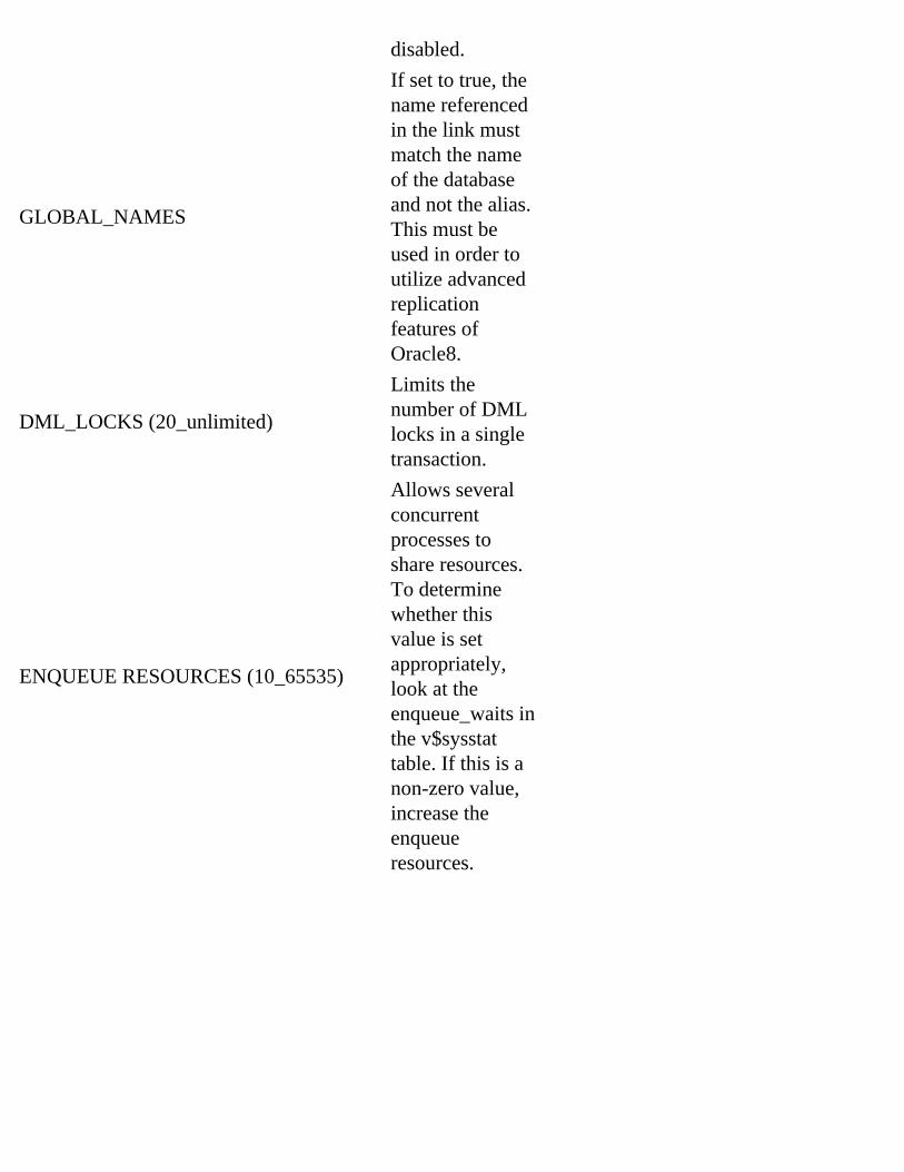
disabled.
GLOBAL_NAMES
If set to true, the name referenced in the link must match the name of the database and not the alias. This must be used in order to utilize advanced replication features of Oracle8.
DML_LOCKS (20_unlimited)
Limits the number of DML locks in a single transaction.
ENQUEUE RESOURCES (10_65535)
Allows several concurrent processes to share resources. To determine whether this value is set appropriately, look at the enqueue_waits in the v$sysstat table. If this is a non-zero value, increase the enqueue resources.

MAX_TRANSACTION_BRANCHES (1_32)
The maximum value for this parameter has been increased from 8 to 32. Branches are the numbers of different servers (or server groups) that can be accessed in a single distributed transaction. Reducing this number may decrease the amount of shared pool used.
OPEN_LINKS (0_255)
The number of concurrent open connections to other databases by one session. In a distributed environment, care must be taken to ensure that this value is not less than the number of remote tables that can be referenced in a single SQL statement. If the value is set to 0, there can be no distributed transactions.
OPEN_LINKS_PER_INSTANCE (0_UB4MAXVAL)
This is new to Oracle8. It limits the number of open links created by an external transaction manager. For more information, refer to your Oracle8 documentation.
Page 712
Identifying Potential Problems with a Distributed System
System changes are the biggest problem in managing a simple distributed system. That is not much different than managing a single, autonomous database. The difference is that each database can see objects in other databases. This creates a system that depends on continuity. Below are the changes within a system that must be coordinated within a distributed system.
● Structural changes. Procedures and triggers used to update or replicate specific remote tables will fail when the remote table is structurally altered or removed. Database links that reference a dropped table will fail.
NOTE
If a user drops a table that is referenced by links from another system, there will not be a referential integrity warning. These warnings occur only when the table contains elements that are referenced.n
● Schemachanges. In addition to tables being removed, the privileges of a user referenced in a database link must have the proper privileges. Changes to profiles and roles must be coordinated to ensure that they will not affect the rest of the distributed system. This includes passwords!
● Changes to the SQL*Net objects. Files such as TNSNAMES, PROTOCOL and TNSNAV will affect the distributed database system.
● System outages. Coordination between outages is crucial, particularly to systems that depend upon distributed updates, snapshots, or replication. In many cases, if this process is broken,

manual intervention must occur in order to repair the problem. Unless a DBA is informed that a database or network is down, the integrity of the distributed system is jeopardized.
Communication between organizations is extremely important, particularly among developers and the DBA. A change in the structure of one database or IP address can affect the entire company and the integrity of the distributed system. This coordination usually is in the hands of the DBA(s).
Another problem can occur if the connection between databases is lost. The responsibility in determining what has happened if connectivity is lost will begin with the DBA. The DBA must be able to easily identify error messages, particularly associated with SQL*Net or Net8. For more information concerning troubleshooting connection problems, please refer to Chapter 20.
Tuning a Distributed System
Tuning methods for a distributed database should be the same as those for an autonomous database. Please refer to Part VIII, "Performance Tuning," and keep the following rules in mind:
● Poorly written SQL will still perform poorly if distributed. ● Remote tables that are partitioned are not seen as partitioned by the local cost-based optimizer. ● Avoid using multiple database links in a single SQL statement.
Previous | Table of Contents | Next

Previous | Table of Contents | Next
Page 727
Chapter 29
Performance Tuning Fundamentals
In this chapter
● Revisiting Physical Design ● Understanding Why You Tune ● Knowing the Tuning Principles ● Tuning Goals ● Using the Return on Investment Strategy ● Revisiting Application Types ● Understanding Benchmarks ● Using Oracle Diagnostic Tools
Page 728
Revisiting Physical Design
We stated in Chapter 3, "Physical Database Design, Hardware, and Related Issues," that physical (and logical) designs are the first steps in tuning a database. This is indeed true. One of the first steps in many tuning books is to tune the design. Well, following proper logical and physical design, you have done just that. If all has gone well, your design should allow your database to perform at more than an acceptable level to begin with. However, there are two things that always creep up with database systems: growth and changing application requirements.
If your database is relatively static, is made up mostly of lookup tables, or for any other reason experiences very little or very slow growth, this factor is not a problem. If, on the other hand, your database is like most others, it will grow over time by some substantial percentage, such as 10 percent or more. Then, despite initially good logical and physical designs, you might periodically need to tune the database to accommodate or otherwise compensate for this growth. In addition, all database systems have fallen prey to the phenomenon of applications, which are in perpetual redefinition. Here is an example you might have come across:
Manager: "The application doesn't work. It's running too slowly. What's wrong with the database?"

Programmer: "The code hasn't changed."
DBA: "The database hasn't changed."
What could be the problem, then? In this instance, the usage has probably changed. This is really only another fancy way of saying that the application requirements have changed. For example, suppose the application originally was intended to allow read-only access to seven tables individually. However, if the application is now being used to join four more tables with some or all of these seven tables to gather more information than originally requested, some tuning might be necessary. In fact, some physical redesign, also known as physical restructuring, might be required.
You can restructure a database physically to improve performance and still permit the application to function as desired. This is possible with Oracle, as with other vendors, because Oracle obeys Codd's rule number 8: physical data independence. So the answer might have been found by consulting with the user:
User: "The application doesn't work? Oh yeah. We're using some different tables now."
There is one other thing, aside from growth and changing application requirements, that will require a DBA's performance tuning skills: the poorly designed database.
With growth and changing application requirements, we had assumed the database was well-designed. Unfortunately, as many DBAs can attest, this is often not the case. Many times a DBA takes over a database system that another DBA has left, is called in to fix the performance of someone else's database system, or is confronted with a database system that is the result of a legacy migration. In cases such as these, what is needed before performance tuning is a logical and physical analysis and redesign. It might be that the database doesn't need much redesign, or it might be that it needs a complete overhaul.
Page 729
In either case, once that design has been ironed out, the DBA can move on to performance tuning proper. However, after the redesign, it might be best to simply put the application to use and do some performance monitoring first. After all, with proper design (or redesign) comes initially good performance. It might very well be that no new additional tuning is required for some time to come. (In practice, I have personally found this to be the case.)
Understanding Why You Tune
Why tune? We have just answered this question. The current database system is not performing acceptably, based on user-defined criteria, for one of the following reasons:
● Poor design

● Growth ● Changing application requirements (possibly including a redefinition of what acceptable
performance is)
When might database tuning efforts not be fully effective? When components that are external to the database, yet vital to the entire client/server application performance, fail to perform acceptably, database tuning might not help without the corresponding tuning of these other application infrastructure pieces. Except for the most isolated, stand-alone, batch production database applications, most modern database systems are client/server based.
The main components external to the back-end database are the back-end operating system (or OS), the network, and the client OS. The major examples are:
● Very weak clients (PCs) ● Network saturation ● Very weak, saturated, or poorly tuned OSs
Clients (PCs) are weak in the sense that they have older CPUs (486 or less), relatively little memory (<= 16MB), and/or little storage (<= 1GB). This especially holds true if the application is "heavyweighted toward the client" and thus requires a fat client. A fat client is one in which a large portion of the application processing is segmented onto the client. A thin client is obviously the opposite of this, with most of the processing taking place at the server end. So, unless an application requires only dumb terminal access or thin clients, weak clients will not suffice.
A network is considered to be saturated by varying definitions. To be saturated means that a system component has reached maximum possible throughput. A 10 Mbps ethernet is considered saturated when it reaches 30 percent of its bandwidth. Networking specialists might handle this in different ways, including resegmenting the network locally, adding more network segments, or changing to a broader-band network media type, such as a 100 Mbps Fiber Distributed Data Interface (FDDI). In any case, we have gone well off the beaten path of database tuning.
An OS might be very weak, just like a client. It is only weak relative to the applications it must support. But in general, modern database servers that have 32-bit processors, 4 processors, 256MB memory, and 10GB of disk space might be considered weak. An OS can be saturated in
Previous | Table of Contents | Next

Previous | Table of Contents | Next
Page 722
unmanageable, the DBA should purge the logs. This can be done via the enterprise management tool, or the DBA can perform this with the stored procedure or API call DBMS_SNAPSHOT.PURGE_LOG. The syntax for this is as follows:
Execute dmbs_snapshot.purge_log(`[master table name]',number,'flag');
number is the number of historical snapshots to remove. If the DBA wants to remove all the logs in the snapshot log, this number should be very high. Care must be taken when using this. If all the logs are removed, the snapshot will have to be completely refreshed. This can be a problem if the table is very large.
NOTE
The flag is an override value. If set to DELETE, then even if the number is set to 0, the logs will be deleted from the least recently refreshed snapshot.n
Understanding Limitations of Snapshots
The initial creation of a snapshot of a large table may be beyond the capabilities of the system. For example, if a snapshot of a large table with several million rows of data had to be replicated over unstable communication lines, it might be better to perform an offline instantiation. To perform this, several steps must be taken. This must be done carefully and, if possible, in a test environment with a great deal of storage space. Use these steps:
1. In the production database, create a snapshot log for each of the master tables (the tables that will have snapshots in the remote site).
2. Using a new schema and in the test database, create a snapshot referencing the production database containing the master table. The name must be unique. Ideally, it should be the name that will be used at the remote site.
3. If this process must be done in the production database (not recommended), the link in the CREATE SNAPSHOT statement will refer to the current database. Oracle refers to this capability as a loopback link.
4. Export the new schema. The same schema as the owner of the new snapshots should perform the export.
5. Drop the newly created snapshots. Be sure that this is done by hand (using API calls). If not, ensure that only the snapshots, and not the corresponding objects, are created.

To create a snapshot at the remote site:
1. Create an empty snapshot group. This is necessary to support the procedure call in the next step. 2. Use the following procedure:
DBMS_OFFLINE_SNAPSHOT.BEGIN_LOAD(gname='[groupname]'.sname=>'snapshotname',)
This will create a snapshot "shell" for the data about to be imported. 3. Import the snapshot base table. This is identified by the preface SNAP$ table.
Page 723
4. Once the import is complete, use the procedure DBMS_OFFLINE_SNAPSHOT.END_LOAD to indicate to the system that the import is complete. The easiest way to visualize this process is the hot backup process, where the command ALTER TABLESPACE BEGIN BACKUP is issued.
NOTE
Just as tables cannot be created using a select on a LONG datatype, snapshots cannot support this select statement.n
Tuning Snapshots
Complex snapshots consisting of multiple table joins can severely degrade performance. It is imperative that the query used to create a snapshot be thoroughly tested and tuned. This includes utilizing explain plan and tkprof prior to creating the snapshot. If required, create several single table snapshots at the child site and then create a view locally based on the physical snapshots. Performance will be significantly enhanced and network traffic will be reduced.
In order to keep the packages used to refresh a database in the library cache, it helps to pin these packages in memory. This will help prevent the package from being removed from memory. To pin a package, call the package and then use the package DBMS_SHARED_POOL. Prior to pinning a package, it must be referenced. The easiest way to reference a package is simply to recompile it. The syntax for this is
ALTER PACKAGE DBMS_SNAPSHOT.I_AM_A_REFRESH COMPILE;
There will be a response:

Package altered.
Now, pin the package with the following statement:
Execute DBMS_SHARED_POOL.KEEP(`DBMS_SNAPSHOT');
The response will be
PL/SQL procedure successfully completed.
This will improve performance. It may not significantly enhance performance, however, it does help—particularly with those snapshots that are frequently refreshed.
Other packages that can be pinned for performance are
● DBMS_REFRESH ● DBMS_REPUTIL ● DBMS_REPCAT ● DBMS_DEFER
For more information on these packages, refer to the Oracle8 Server Replication—Replication Manager API Reference.
Page 724
Using Initialization Parameters for Snapshots
The init.ora table contains several parameters that directly impact the snapshot process. These parameters are defined in Table 28.2.
Table 28.2 Initialization Parameters for Snapshots
Parameter Description
JOB_QUEUE_INTERVAL (1_3600)
The interval that the snapshot process wakes up. Care must be taken to ensure that this is not set so high as to interfere with the interval of the snapshot itself.

JOB_QUEUE_PROCESSES (0_36)
Limits the number of processes for the snapshot process. Normally, one should be sufficient unless there are several snapshots or large snapshots that may interfere with the snapshot process.
Page 725
PART VIII
Performance Tuning
29. Performance Tuning Fundamentals 30. Application Tuning 31. Tuning Memory 32. Tuning I/O
Page 726
Previous | Table of Contents | Next

Previous | Table of Contents | Next
Page 719
● LOB_storage_clause is related to the Large Object Definition. For more information on Large Objects, please refer to Oracle8 Server Application Developer's Guide.
● LOGGING/NOLOGGING specifies whether redo log information is to be written when creating an index. This is similar to the CREATE INDEX NO RECOVER command. It also affects direct loading and direct load inserts. This can significantly affect the index during recovery. For more information on this, read the GREAT INDEX command in the Oracle8 SQL documentation.
● CACHE/NOCACHE specifies whether the snapshot will be kept in memory after a full table scan. For more information on this, read the Oracle8 Concepts Guide concerning memory structures, cache, and the LRU algorithm.
● WITH PRIMARY KEY is a default in Oracle8. By specifying the creation of a primary key snapshot, the master table can be reorganized without impacting a fast refresh. There are some limitations concerning utilizing a PRIMARY KEY snapshot. There must be a primary key in the table referenced. This must be by using the PRIMARY KEY constraint of the CREATE TABLE command. All columns within the primary key must be used.
CAUTION
If the primary key is not used with the create snapshot command, the record's rowid will be used. This can create potential problems if the master table is recovered due to a database recovery. The recovery will change the rowid values and can potentially invalidate the snapshot. To ensure that this is not a problem, refresh snapshots using the complete option after any database recovery.
Using defaultmaster|LOCAL specifies which type of rollback segment to use. DEFAULT will enable Oracle to choose, MASTER will use the rollback segment at the remote site, and LOCAL will use the rollback segments in the local database.
Using Snapshot Refresh Groups
Many snapshots, although associated with different master tables, may have the same refresh rate, making them candidates for grouping. Although Oracle8 enables a point-and-click method for creating these snapshots, it is important to know what happens behind the mouse.
Oracle refers to this capability as API calls. The manipulations of replicated objects are not performed

via standard SQL commands. The calls are performed through the use of procedures. For more information concerning procedures, their syntax, and how they are used, refer to the Oracle8 Application Developer's Guide.
Identifying Potential Problems with a Snapshot
As with any database management process, proactive management is the most appropriate method. To proactively manage the snapshot process, the DBA must be able to identify potential problems and design the system in order to prevent them from occurring. This section identifies some of these problems.
Page 720
Sizing There is one pitfall to avoid during the creation of a snapshot. Although it is query only, the snapshot is not a static table. Sizing should be based on the update rate of the table copied, not the snapshot itself. For example, if the table GERMANY_SPECS is a highly dynamic table, it should have a larger percent used (PCTUSED) to accommodate the updates. The table should be sized to ensure that fragmentation does not occur.
Dropping Objects Inadvertently Some of the snapshots are in refresh groups. To find the job numbers associated with them, query the DBA_REFRESH_CHILDREN table. These groups can be dropped; however, care must be taken to ensure that the objects are not also dropped. For this reason, the method for dropping any type of replication group should be performed via sql code and not the Enterprise Manger. The Enterprise Manager enables the DBA to drop the objects by simply clicking on the objects. The way to drop Refresh Groups is to use the procedure:
execute DBMS_REPCAT.DROP_SNAPSHOT_REPGROUP(gname=>'[name ofÂgroup]',drop_contents=>FALSE);
drop_contents defaults FALSE; specifically setting it to FALSE is just an added precaution. When using procedures, they must be entered as a single line or they will not be invoked.
CAUTION
If you set drop_contents to TRUE, the tables associated with the group are also dropped.
Losing Snapshot Refreshes When a master database cannot complete the refresh of a snapshot, it will try 16 more times before the refresh attempts will stop. The 16 times does not mean 16 refresh intervals. The first time a refresh fails, the snapshot process will wait one minute and try again. If that fails, the time doubles to two minutes, then four, and the time span grows exponentially until it reaches or exceeds

the actual refresh interval. When that occurs, it will continue at the refresh rate. After 16 times, Oracle will update the column BROKEN in the tables USER_REFRESH and USER_REFRESH_CHILDREN. The broken column indicates that something has gone wrong with the snapshot refresh. This will not only be reflected in this table, but the Oracle SNP process will also indicate a refresh problem in trace files and alert.log.
One way to reduce the possibility of a broken snapshot is to create the snapshot with the FORCE option rather than FAST. FORCE will choose FAST unless something has occurred to prevent a successful FAST refresh; then it will perform a complete refresh instead. One drawback to using this option occurs in the event of a very large table. If the refresh takes a long time, problems may occur if the current refresh is still going when the next refresh is scheduled to occur.
After the DBA has determined that the refresh is broken and has rectified the problems that broke the snapshot, the snapshot can be manually refreshed. Oracle8 provides several methods of refreshing manually. One way is to execute the job defined as the snapshot. To determine this, log in at the child site and perform the following query:
SELECT RNAME,JOB FROM DBA_REFRESH;
Page 721
The results will be similar to this:
RNAME JOBGERMANY SPECS 142
Run the job that has the broken snapshot. The job name will be the same as the snapshot (locally/child). To perform this, use the following procedure:
Execute DBMS_JOB.RUN(142);
The response will be the following:
PL/SQL procedure successfully completed.
When this has been completed, verify that the BROKEN status of the tables USER_REFRESH and USER_REFRESH_CHILDREN is no longer Y. If the broken status remains at Y, repeat the process again. If this does not fix the problem, ensure that there are not other problems (such a loss of connectivity) that is preventing this refresh from occurring.
To proactively monitor the refresh process to prevent another broken snapshot, compare the snapshot time and the time in the snapshot logs. These should match; if they do not, it may indicate that the

problem causing the initial loss of the snapshot has not been completely resolved.
At the master site, use the following query:
Select master,substr(to_char(current_snapshots,'MM-DD-YYYY HH:MI:SS'),1,20)time FROM DBA_SNAPSHOT_LOGS;
From the local/child site, use the following query:
SELECT NAME,SUBSTR(TO_CHAR(LAST_REFRESH,'MM-DD-YYYY HH:MISS'),1,20)TIME FROM DBA_SNAPSHOTS;
These times should match. If they do not, the snapshots will still require manual management until the problem has been completely resolved.
Controlling Snapshot Log Growth Snapshot logs contain the DML changes of the master snapshot. This determines what should be sent to the remote sites. The log is purged after all of the snapshots using this log have been completed. However, if there is a problem with the snapshot, or one of the snapshots is refreshed infrequently, then the snapshot log can grow uncontrollably. This can present a problem in two ways. The DBA should size the logs to enable a certain amount of growth. If the stability of the snapshot is mission-critical, the use of unlimited extents is recommended. This will remove the possibility of reaching the maxextents. This fills the tablespace where the log resides. The DBA should periodically check this log to ensure that this does not occur. If the size of the log is becoming
Previous | Table of Contents | Next

Previous | Table of Contents | Next
Page 730
various ways, just as a network can. Under heavy load (many concurrent users and/or huge amounts of data being moved), an OS's CPU, I/O, and/or memory might be saturated.
Another way of putting this is that when a component is saturated, the system is bottlenecked on that component. Hence, if the CPU of a UNIX machine is saturated, such as with a utilization of >= 85%, the UNIX system is said to be bottlenecked on the CPU, or simply CPU bound.
Lastly, an OS might just need some re-tuning. If, for example, a DSS requires only very large files to be stored on disks, a system administrator (SA) can tune the UNIX file system so that it optimally stores very large files in contiguous chunks.
As you'll see in Chapters 31 to 33 and Appendixes A to C, tuning a database system is heavily intertwined with tuning the OS. It is a good thing to be both an SA and a DBA, because you don't have to ask permission to do this or that. You just do it. However, in practice, DBAs often have to fight battles with SAs and management over resource allocation and tuning issues. My recommendation is to gather quantifiable proof through Oracle diagnostic tools, discussed later in this chapter (see the section "Using Oracle Diagnostic Tools") and in Chapters 31 to 33, and use those figures to justify your resource needs.
Knowing the Tuning Principles
Now is a good time to enumerate the major performance tuning principles you will find in almost any performance tuning reference.
What are the major performance tuning principles? They are as follows:
1. Divide and conquer. 2. Preallocate, prefetch, and precompile. 3. Triage. (Be proactive.) 4. Bulk, block, and batch. 5. Segment the application appropriately.
If these look familiar, they should. They are the physical design principles we discussed in Chapter 3, with a slight twist on numbers 2 and 3. Let's look at a few scenarios regarding how these principles apply to performance tuning per se, and not just physical database design.

Tuning Principle 1
Divide and conquer is the principle. In essence, you want to use parallel techniques as a remedy for a bottleneck.
Follow along with this scenario: If performance monitoring shows that the database system has a heavy concentration of physical reads and writes to one particular disk, that disk is a bottleneck. The physical and logical structures of Oracle, for example, need to be separated to allow parallel access. As often is the case, what is happening here is that an application has several users or processes trying to access the same tables or tablespaces on that disk.
Page 731
Frequently, tables that must be joined together might exist on the same disk. This makes for poor performance.
The OS must access the disk on Oracle's behalf for some blocks of the table's data, perform this cycle again for the second table, and repeat the whole process for all the blocks of both tables until Oracle has joined the two. What happens at the hardware level is that the read/write head of the disk must read the requested sectors (physical data blocks) of the first table, reposition itself to read the requested sectors of the second table until a match is found, and then repeat. Access time (in milliseconds) of a disk consists of seek time and latency (rotational delay). Seek time is the repositioning of which we spoke, when the read/write head must move inward and outward along the radius of the disk to find the track containing the requested sectors. Seek time dominates the latency, or the time it takes for the disk to spin around to access the sectors.
The important thing is that joining two or more tables on the same disk requires a high proportion of seeks to reads. As a DBA, your goal is to reduce the number of seeks. You want to minimize contention and get rid of this bottleneck. To do this, you separate the tables that are being joined onto different disks. This same methodology holds true for tables that coexist on the same disk and can be simultaneously accessed even though they aren't being joined together. The result is the same: bottleneck. The solution is the same: separate them.
By the way, RAID is susceptible to this scenario just as easily as a standard disk. At first, it might not seem possible that RAID, especially levels 1, 3, and 5 (which we discussed in Chapter 3), could suffer this same type of problem. Quite clearly, striping a single table across several disks (a RAID volume) will undoubtedly increase performance. However, if this table is stored on the same RAID volume with tables that must be joined with it or at least are accessed concurrently, we have the same problem: bottleneck. Again, the solution is the same: separate them.
The reason you still have the bottleneck is not so clear at first glance, but think about it. Chunks of all the tables (stored in the data files of their respective tablespaces) are striped across all the disks of that

RAID volume. Although no single table exists in its entirety on any one disk, chunks of all tables coexist on all of the disks. Hence, we have the same problem on a smaller scale. Rather than separating joined or otherwise simultaneously accessed tables onto different disks as with standard disk setups, we separate the tables onto different RAID volumes.
Tuning Principle 2
Preallocate, prefetch, and precompile is the principle. Do work ahead of time whenever possible.
Follow along with this scenario: Suppose you have a database system that is particularly volatile. It grows and shrinks considerably and frequently. In fact, as an application type, it can be called a VCDB. When you access the database during the non-growth period, performance is reasonable. However, during its growth phase, performance is very poor, especially early on.
Page 732
What is likely happening here is that dynamic growth is slowing down the online system. In Oracle terms, this is known as dynamic extension. Rows are being updated or inserted such that Oracle must extend or allocate the next extent for a table, as designated by the storage clause when either created or altered, or take the tablespace default. In either case, the table had enough space at creation time up until this most recent growth period and then had to extend to accommodate it. Of course, simply having a table extend in Oracle is not the end of the world. Far from it. It is, in fact, a normal course of events.
However, when a table is frequently extending, especially for large amounts of data, and causing online access to suffer, it's a major problem. Concurrent users shouldn't have to suffer. For database systems of this type that require frequent or very large data extents, preallocation is best. You want to create your table with sufficient storage to begin with—that is, to handle the maximum expected peak size. In the storage clause of your table (or tablespace) create statement, set your INITIAL extent size, your NEXT extent size, and then set MINEXTENTS so that INITIAL + ((MINEXTENTS - 1) x NEXT) equals the maximum expected peak size of the table.
Tuning Principle 3
Triage is the principle. Attack the most important problems first to get the greatest return on investment.
Follow along with this scenario: You have a slow batch system. When you do production runs, the system crawls. Upon reviewing the SQL code that makes up the application, you seem to have several very inefficient programs that could be rewritten. To do so might take about two months. You then analyze performance monitoring statistics and find that rollback shows high contention, apparently because you are running several concurrent programs at once to help speed up the runs. You fix the rollback by adding more segments, but you gain little increase in your elapsed times. What to do?

No matter how well you tune the back end, the front end (or application code) dominates the total time usage of a client/server system, not accounting for networking and other issues. You must tune the application first and then tune the database. The investment of two months will be well worth it when the production runs finish faster than ever.
If this can't be done for some reason, other database efforts such as logical or physical restructuring can be done as a temporary measure. But this truly shouldn't be done at all; you'd be changing your good database design because of a poor application design. You wouldn't gain much with that approach.
Tuning Principle 4
Bulk, block, and batch is the principle. When appropriate, group things together that are processed together and don't compete with one another for resources.
Follow along with this scenario: Your DSS provides real-time, read-only information to external analysts via the Internet. You have a Web page as a front end to our database system. Concurrency is sometimes medium high (up to 100 users) but does not seem to cause problems. What you have had complaints about is the throughput from selecting from large tables.
Previous | Table of Contents | Next

Previous | Table of Contents | Next
Page 733
You have a classic case here. When selecting most or all of the rows from a table, the optimizer must choose a full table scan over any indexes as its access path. This in itself cannot be avoided if that is what the user desires, and this type of access is part of the application requirements. What can you do to speed things up? Well, you can initially set your DB_BLOCK_SIZE to 4KB on your UNIX system. You can increase this to 16KB or 32KB. The larger the block, the more cost effective your reads are. In other words, you get more rows of data per block with each read. Hence, you can make the reads more efficient by increasing block size for large data retrievals.
You can also consider increasing DB_FILE_MULTIBLOCK_READ_COUNT and DB_BLOCK_BUFFERS as necessary. Reading more blocks at once and increasing block buffering should also help in DSS cases, but we'll discuss these later in Chapter 32, "Tuning I/O."
Tuning Principle 5
Segment the application appropriately is the principle. Assign the various pieces of the application to the appropriate places (the client, the middle tier, or the server).
Follow along with this scenario: You have a client/server database system that does order entry and control. However, the order entry screens themselves tend to run slowly on the PCs. Response time is poor, and the application seems to burden the client because a single entry might take seconds (which is slow, in terms of response time).
This could be anything. You first need to examine how the application is partitioned. It turns out that most of the data validation is done in the front-end code, and this might be the culprit because it accounts for a large majority of the lines of code. Most of the front-end code algorithms go like this:
1. Clerk logs in to the database. 2. Clerk reads data from some tables. 3. Clerk enters data into the screen. 4. Clerk waits while the front end validates entered data in some tables with other tables. 5. Clerk logs out if done or repeats steps 2 through 4 if not.
The problem with this is that the clerk's transaction is active the entire time, and it interactively validates data among tables from the front end. This validation process (step 4) should take place on the server, non-interactively. It belongs there because it deals directly with the data. Processes should normally be located as close as possible to the data on which they operate, unless there is some compelling reason to do otherwise (such as that the server is underpowered). A standard way to segment the preceding

application is to divide it into three major steps: read (the input data) with a transaction, change locally (interactively) without a transaction, and write back the changes (the output data) with a transaction. This application segmenting is also known as transaction chopping. If done correctly, it should result in a substantial reduction in response time.
Page 734
Tuning Goals
There are different ways of determining the goals of a performance tuning effort. A DBA should consider them all. Consider your application type, which we discussed in Chapter 3 and will discuss again later in this chapter (see the section "Revisiting Application Types"). Database systems can be sampled on various quantitative measures, which we also discussed in Chapter 3 and will discuss in "Understanding Benchmarks" later in this chapter. The most important of these are
Throughput. Work per unit time, as measured by transactions per second (tps); higher is better. Response time. The time it takes for an application to respond, as measured in milliseconds or seconds; lower is better. Wall time: The elapsed time a program takes to run; lower is better.
In any system, throughput and response time usually run counter to one another as tuning goals. If response time is high (poor), throughput might be high (good). If throughput is low (bad), response time might be low (good).
Common sense helps when sorting out these two conflicting measures. The more users that are concurrently using a system within a certain amount of time, the more likely it is that each user will experience longer delays than normal, but the number of transactions going through the system will be greater. On the other hand, if you decrease the number of concurrent users accessing the system within a certain time window, each user will enjoy faster response time at the expense of fewer overall transactions being completed in that duration.
Typically, OLTP systems want low response time or high throughput, in terms of transactions per second, depending on the application needs. A DSS wants low response time. However, a DSS also might want high throughput in terms of blocks read or written per unit time. This type of throughput is not necessarily counterproductive to high concurrency and low response times. A batch (production) system typically wants lower wall times. For example, everyone likes for the payroll application to complete on time!
Always consider the two central tuning goals:
Maximize your return on investment. Invest your time and effort wisely by working the

problems most likely to yield the most improvement. Minimize contention. Bottlenecks are characterized by delays and waits; eliminate or reduce these whenever possible.
Finally, consider the following general-purpose database tuning goals:
Minimize the number of blocks that need to be accessed; review and rewrite code as necessary. Use caching, buffering, and queuing whenever possible to compensate for the electromechanical disadvantage (memory is faster than disk); prefetch. Minimize the data transfer rates (the time it takes to read or write data); fast disks, RAID, and parallel operations help do this.
Page 735
Schedule programs to run as noncompetitively as possible; they might run concurrently and yet still be noncompetitive for the most part.
Using the Return on Investment Strategy
The return on investment (ROI) strategy is a top-down, cost-effective way of viewing the performance tuning process. It helps you find the best way to approach the tuning of your particular application. We have seen ROI turn up before as one of the major performance tuning principles (triage) and as one of the two major performance tuning goals. Now we take it to heart and use at as a high-level, step-by-step methodology for performance tuning.
You want to do performance tuning in the order that gives you the greatest gain for your time and effort. In the ROI strategy that follows, notice that steps 1 through 3 amount to logical and physical design, which were covered in Chapters 1, "Databases, DBMS Principles, and the Relational Model," and 2, "Logical Database Design and Normalization." Logical design is regardless of DBMS vendor. Hence, there are no Oracle specifics when dealing with logical design (not counting logical design tools). We'll revisit application types in the next section and apply some Oracle-specific recommendations for physical design and performance tuning recommendations for these applications. In the later chapters, we'll revisit these performance tuning recommendations for Oracle more closely, looking at tuning the application, tuning memory, and tuning I/O.
Steps 4 and 5 amount to tuning the application, which we'll cover in Chapter 30, "Application Tuning." Steps 6 and 7 amount to tuning memory and are included in Chapter 31, "Tuning Memory." Lastly, steps 8 and 9 amount to tuning I/O and appear in Chapter 32. Steps 10 and 11 deal with components even more external to the database than the OS: the network and the client. Step 12 offers some advanced and less-common solutions, which should be tried only after standard methods have been applied and the desired performance gains have not been realized (steps 1 through 11). Chapters 30, 31, and 32 contain

Oracle specifics to help you do proper performance tuning.
For now, let's review the steps in a little more detail, in descending order of return on investment.
Step 1: Do a Proper Logical Design
As covered in Chapter 2, you can reduce storage. In practice, this often means more tables with fewer rows per table. In turn, this means the capability for faster searching. The fewer rows that are stored and must be searched through, regardless of the searching technique, the quicker you'll be able to find what you're looking for.
Step 2: Do a Proper Physical Design
In Chapter 3, we offered a general-purpose hardware layout. In the section "Step 12: If All Else Fails, Consider More Exotic Solutions," we'll offer some more application-specific twists to this general hardware layout.
Previous | Table of Contents | Next

Previous | Table of Contents | Next
Page 749
Chapter 30
Application Tuning
In this chapter
● Motivation ● Understanding the Optimizer ● SQL Trace and tkprof ● Understanding EXPLAIN PLAN ● Identifying Typical Problems ● Rewriting Queries ● Introducing New Index Features for Oracle8
Page 750
Motivation
Tuning the application really amounts to tuning your SQL statements within your application. If your application has a graphical user interface (GUI) front end, tuning the application still amounts to tuning analogs of SQL statements. In other words, all the GUI-level actions can be mapped to one or more SQL statements (SELECT, INSERT, UPDATE, DELETE) of varying complexity. In any case, our Return-on-Investment (ROI) strategy tells us that we must tune the application first, if at all possible, then resort to tuning all the aspects of the database last.
Subjective estimates have shown applications being responsible, on average, for 80 percent of the total system (application+database) performance, leaving only 20 percent for the database. I agree with the idea behind this claim, as we have just covered. However, I tend not to agree with the numbers that make up this claim. In my experience, I have seen systems that fulfill these estimates and systems that exhibit the opposite situation—the opposite situation being the database accounting for most if not all the performance.
What this really means to DBAs is that the performance of systems may be labeled situational, relative, or application specific. This should sound familiar, especially in regard to discussions of application types. Yet one absolute rule does hold true, and I wholeheartedly advocate that DBAs pay close attention to the first rule of tuning: The application should always be tuned first.

This holds true for two reasons: (1) The majority of database systems existing today owe most of their performance to their applications, and (2) Even if this does not hold true for your individual system, as a DBA you must categorize the system's application type. This means that you must review the application, specifically the types of transactions: the access code and the SQL code. Even if your application code is programmed as efficiently as possible from a database access point of view, you must still understand how the programs interact with your database.
How do you accomplish the task of reviewing the application? If the application is reasonably small—in terms of lines of code or number of separate program units (modules)—then manually reviewing everything is possible. On the other hand, if the application is large, full-manual review would most likely be out of the question. Principle 3, Triage, of our Performance Tuning Fundamentals (Chapter 29) gives us direction. You can focus on those modules or sections of code that tend to account for most of the resource and time consumption.
First you will attempt to fix the 20 percent of the application code that accounts for 80 percent of the system performance. (Then you can work on the remaining code to squeeze out the rest of the performance potential, if you have time and personnel to do so.) How do you actually do this? The sections following the next one discuss the Oracle tools that you will need. But first, the next section gives you the necessary background to use those tools—an understanding of the Oracle optimizer and how it works.
Page 751
Understanding the Optimizer
An optimizer is a piece of software and part of an RDBMS that is responsible for optimizing, or formulating, the most efficient way for a given SQL statement to access the data. To do this, the optimizer chooses a sequence of access paths that provide the (hopefully) fastest way for Oracle to get to the data and then builds the execution plan based on those access paths. An access path is a physical way to the data. An execution plan is the sequence of Oracle executable steps that follows the chosen access paths.
The technology behind the Oracle optimizer, as with many other RDBMS vendors, has advanced considerably over the past few years. Ironically, the optimizer still may not always provide the best way (the optimal way) to access data. In older versions, the programmer had to be careful about how she coded her SQL statements. With the knowledge that the ordering within a SQL statement could drastically affect how it would perform, programmers had to do a lot of manual optimization. Likewise, the DBA had to be aware of this situation. The better the optimizer, the less optimization responsibility is on the users, programmers, and DBAs. Even with the current field of RDBMS optimizers, programmers still need to know optimization techniques and apply them when possible. However, programmers don't need to be quite as expert about the optimizer as before. DBAs should always remain

aware of the optimizer technology, optimization rules, and proper optimizer usage.
Optimizers come in two flavors:
● Rule-based—A rule-based optimizer chooses the access paths based on a static, RDBMS vendor-specific rank-ordering of those access paths that are the fastest ways to the data. Although the rankings are vendor specific, it is relatively easy to compare and map analogous access paths between the output of different vendors' optimizers.
● Cost-based—A cost-based optimizer chooses the access paths based upon some data-distribution statistics stored internally, usually within the RDBMS data dictionary. Typically, the DBA must periodically run some RDBMS commands to maintain these statistics.
Oracle's 7.x and higher optimizers offer both rule-based and cost-based optimization capabilities within the same optimizer. Oracle's 6.x optimizer offers rule-based, but does not have a fully automatic cost-based optimization. All these versions offer a programmer an override known as a hint. It is not a true override, in the sense that the optimizer does not always follow the hint. Consider a hint a suggestion to the optimizer. If no syntax errors exist, the optimizer should generally follow it. A hint is placed inline, meaning directly in the SQL statement code. Listing 30.1 shows a SELECT statement that suggests to the optimizer to use the INDEX on the table from which it is selecting:
Listing 30.1An Example of a Query with a Hint
SQL> SELECT /*+ INDEX */ EMPLOYEE_ID 2> FROM EMPLOYEES 3> WHERE EMPLOYEE_ID = 503748;
Previous | Table of Contents | Next

Previous | Table of Contents | Next
Page 748
Previous | Table of Contents | Next

Previous | Table of Contents | Next
Page 745
Using Oracle Diagnostic Tools
Your major Oracle diagnostic tools are as follows:
● SQL_TRACE and TKPROF ● EXPLAIN PLAN ● The V$ dynamic performance views and Server Manager line mode ● Server Manager Monitor (GUI) ● The Performance Pack of Enterprise Manager ● utlbstat/utlestat and report.txt ● Third-party products
Using SQL_TRACE and TKPROF
To tune applications, you can use SQL_TRACE and TKPROF. You must set the init.ora parameter TIMED_STATISTICS=TRUE to get timing information. The timing is good to 1/100 of a second. Real-time database systems might have to use alternative timing methods, such as writing your own timer or sampling the real-time OS clock on which the database system resides. You can optionally set the USER_DUMP_DEST to the directory of your choice, and also set MAX_DUMP_FILE_SIZE to the maximum number of bytes you want your trace file to grow. Set SQL_TRACE=TRUE at either the system level (for all sessions), through the init.ora parameter, or at the session level through ALTER SESSION SET SQL_TRACE=TRUE;.
Execute the application, and then set SQL_TRACE back to FALSE if desired. In effect, you're not planning on running the application for timing purposes again in the near future. Use TKPROF to format the trace file. (The TKPROF utility is run from the command line.) Statistics gathered include the query execution cycle component times (parse, execute, and fetch) and logical versus physical reads. The usage, syntax, and interpretation of SQL_TRACE and TKPROF will be covered in detail in Chapter 30.
Using EXPLAIN PLAN
Another application tuning tool is EXPLAIN PLAN. You must run utlxpln.sql to create the PLAN_TABLE, or create it yourself interactively. EXPLAIN PLAN FOR <SQL statement>; will explain the execution plan for that SQL statement without executing it. (This is similar to the NO EXEC option with some other interpreted languages.) You can use this with or without SQL_TRACE and TKPROF. I recommend you review the code first (read it), run SQL_TRACE with TKPROF next, and then use EXPLAIN PLAN last if you're still having difficulty with an application that's performing

poorly. This will be addressed in Chapter 31, along with how the Oracle optimizer works, which will help explain how EXPLAIN PLAN works.
Using the V$ Dynamic Performance Views
To help tune memory (Chapter 31) and tune I/O (Chapter 32), all of the Oracle products, such as SQL*DBA, Server Manager, and Enterprise Manager, rely on the V$ dynamic performance views. These views are grouped into instance, database, memory, disk, user, session, and
Page 746
contention aspects of performance. They are based on the internal X$ base tables. DESCRIBE V$FIXED_TABLE and SELECT the columns you want from the V$FIXED_TABLE table to get a listing of the V$ views. The X$ tables are typically not queried directly. Their names and contents change from version to version and within a version.
The V$ views are called dynamic because they are populated at instance startup and are truncated at shutdown. The V$ views (and X$ tables) also form the basis of the standard Oracle tuning scripts, utlbstat/utlestat, which query them using SQL scripts and format the output that is returned. Therefore, if utlbstat/utlestat do not give you what you want, you can use Server Manager and the V$ views to either supplement or supplant those utilities. The least common denominators for all Oracle platforms, older and newer, are SQL scripts, V$ views, and either SQL*DBA or Server Manager line mode (svrmgrl on UNIX, and svrmgr23.exe on Windows NT, for example). This means that if you have developed your own performance scripts, you can run them within these command-line utilities. And there's always SQL*Plus, of course.
Using the Server Manager Monitor
The Server Manager Monitor, which is becoming obsolete because of the advent of Enterprise Manager, offers several screens relating to performance. These screens monitor the MultiThreaded Server, logical and physical I/O, process information, locks and latches, shared pool information, and rollback information. The screens are updated in real time and, as mentioned, are based on the V$ views and X$ tables.
Using the Performance Pack of Enterprise Manager
Enterprise Manager's Performance Pack is extremely useful. It offers several components that can save a lot of time over command-line methods and scripting, especially for experienced DBAs or those who know precisely what to look for. Enterprise Manager allows you to quickly get to that information. The statistics are based on the V$ views and X$ tables but are reformatted into a much more readily digestible GUI form.

The components in the Performance Pack help analyze your logical and physical design. They also monitor locks, a variety of performance issues (throughput, redo, rollback, I/O, memory, and so on), the top user sessions with regards to resource consumption, your tablespace storage (data files, fragmentation, and so on), and application events through tracing.
Using utlbstat/utlestat and report.txt
The most commonly used Oracle diagnostic utilities by far are the utlbstat/utlestat pair. A DBA runs utlbstat before running his or her application or simulation. The utlbstat.sql script builds the beginning tables necessary to collect and store the performance data. Then the DBA runs utlestat.sql, which builds the ending tables and the difference tables, computes the performance differences (the deltas) between the utlbstat run and this utlestat run (in effect, the application duration), formats the output data (including comments and some explanations), and writes it to the default file, report.txt. This file must be interpreted
Page 747
by the DBA, either directly or indirectly (by taking some of the output values given and using them as inputs into simple formulas).
Interpretation of this data means comparing these final figures to more or less established guidelines, keeping the ROI strategy in mind, and categorizing the findings as acceptable or not for that given area of performance. The output in report.txt nearly covers all the bases, either directly or indirectly. So a DBA must simply apply the ROI strategy, the established guidelines, and his or her application knowledge and determine whether or not the memory performance is acceptable, the I/O performance is acceptable, and so forth.
Using Third-Party Products
We've presented a fairly high-level overview of the major Oracle diagnostic tools. Third-party performance monitoring tools exist, and they have relatively large market shares within the installed Oracle customer base. Some examples include offerings from BMC, Platinum, and Compuware. We'll use utlbstat/utlestat and report.txt as our diagnostic tools for Chapters 31 and 32. And, of course, we'll use EXPLAIN PLAN and SQL_TRACE with TKPROF for the next chapter.l
Previous | Table of Contents | Next

Previous | Table of Contents | Next
Page 752
Notice that the hint immediately follows the SQL command (SELECT, INSERT, UPDATE, DELETE). The hint comment, like any regular SQL*Plus comment, begins with a /* and is immediately followed by a plus sign (+), to make /*+ the start of a hint comment. The usual */ ends the hint comment. Also consider how the optimizer knows which index to use if more than one exists, especially if, for some reason, more than one exists on EMPLOYEE_ID. In the previous example, only /*+ INDEX */ is stated, and it is assumed that only one (primary key) index exists for this table. Hence, for this listing, there is no ambiguity. In cases where there is ambiguity, you would need to include the table and index name in the hint to give the optimizer specific information. Hints are discussed in more detail in the following sections.
NOTE
The optimizer will accept only one hint per statement or statement block. The optimizer will ignore any additional hints. Further, the optimizer will ignore any misspelled hints. There is no reported error, and you would have to use Explain Plan, discussed later in this chapter, to determine whether or not your hint was followed.n
Ranking Access Paths
The Oracle 7.x optimizer access paths, ranked by fastest to slowest, top down, are shown in Table 30.1.
Table 30.1Oracle Optimizer Access Paths, Rank-Ordered
Rank Access Path
1 single row by ROWID
2 single row by cluster join
3 single row by hash cluster key with unique or primary key
4 single row by unique or primary key
5 cluster join
6 hash cluster key
7 indexed cluster key
8 composite key
9 single-column indexes

10 bounded range search on indexed columns
11 unbounded range search on indexed columns
12 sort-merge join
13 MAX or MIN of indexed columns
14 ORDER BY on indexed columns
15 full table scan
Source: Oracle Corporation.
Page 753
So, when the Oracle optimizer is following the rule-based strategy, it uses the fastest access paths that fit the given query. For example, Listing 30.2 shows the same query from Listing 30.1 without the hint, and it has been modified with a > WHERE clause.
Listing 30.2An Example of a Query Without a Hint and an Unbounded Range Search
SQL> SELECT EMPLOYEE_ID 2> FROM EMPLOYEES 3> WHERE EMPLOYEE_ID > 500000;
If Oracle were using rule-based as its strategy and a primary key index existed on EMPLOYEE_ID on the table EMPLOYEES, it would use access path #11 (unbounded range search on indexed columns) for Listing 30.2 because the WHERE clause is unbounded. In other words, a WHERE clause is unbounded when it has a greater than (> or >=) operator and no corresponding less than (< or <=) operator, or vice versa. The range is not known until execution time.
If the WHERE clause is bounded (in effect, it has both operators), the finite range is known at parse time. To make an unbounded WHERE clause bounded, you could use the literal maximum (if you knew it), or at least the theoretical maximum for that column according to your business rules. However, you probably wouldn't want to use the MAX operator in addition to your original unbounded range search—if you look at the rank ordering, using MAX is #13, which is below our objective of improving an unbounded search (#11) to a bounded one (#10). Using the MAX operator with your original unbounded range search would only slow you down. But using the actual maximum, if statistically known, would do the trick. Follow these dos and don'ts, which are illustrated in Listing 30.3:
● Do use an actual maximum value (literal) known ahead of time. This is illustrated in the first query of Listing 30.3 (678453).
● Do use a theoretical business maximum value (literal) known ahead of time if the actual is not known. This is illustrated in the second query of Listing 30.3 (999999).
● Don't use the MAX SQL aggregate function because it will only slow things down. This is

illustrated in the third query of Listing 30.3.
Listing 30.3Following the Dos and Don'ts of Rewriting an Unbounded Search to Make It Bounded
SQL> SELECT EMPLOYEE_ID 2> FROM EMPLOYEES 3> WHERE EMPLOYEE_ID > 500000 AND EMPLOYEE_ID <=678453;
SQL> SELECT EMPLOYEE_ID 2> FROM EMPLOYEES 3> WHERE EMPLOYEE_ID > 500000 AND EMPLOYEE_ID <=999999;SQL> SELECT EMPLOYEE_ID 2> FROM EMPLOYEES
3> WHERE EMPLOYEE_ID > 500000 AND EMPLOYEE_ID <= MAX(EMPLOYEE_ID);
Page 754
Analyzing Queries to Improve Efficiency
To no surprise, this general field of attempting to reformulate or rewrite queries to improve their efficiency is known as query rewriting. Query rewriting is covered in more detail in the sections "Identifying Typical Problems" and "Rewriting Queries." Our previous examples are standard fare and easy to understand. For example, to get the maximum (MAX) of a set of values in a column, it would seem to take close to the amount of time of a full-table scan—regardless of whether or not the column was indexed. And, as you can see by the rank ordering of the MAX access path, this seems to be the case. However, there are far less understandable and more exotic ways of rewriting queries that are not as obvious.
Now that you've studied rule-based optimization, what about cost-based optimization? Take a look at the two queries in Listings 30.4 and 30.5.
Listing 30.4 First of Two Similar Queries on the Same Table
SQL> SELECT EMPLOYEE 2> FROM EMPLOYEES 3> WHERE EMPLOYEE_TYPE='VICE PRESIDENT';
Listing 30.5 Second of Two Similar Queries on the Same Table

SQL> SELECT EMPLOYEE 2> FROM EMPLOYEES 3> WHERE EMPLOYEE_TYPE='PROGRAMMER';
Now, suppose you have a relatively large software company with six vice presidents and about 2000 programmers out of about 6000 total employees. The two preceding queries will explain the difference between rule-based and cost-based query optimization and why cost-based optimization is preferred. Assuming you have a non-unique index on the column EMPLOYEE_TYPE, rule-based optimization chooses access path #9 (single-column indexes) for both queries. On the other hand, cost-based optimization—given the data distributions that programmers account for 1/3 of the total number of rows and that vice presidents account for only 1/1000—chooses to use the non-unique index for the query in Listing 30.4, yet is intelligent enough to opt for the full-table scan (the worst case access path #15) for the query in Listing 30.5. The intelligence comes from the stored knowledge of the data distribution.
If the optimizer must access a significant fraction of all the rows of a table, a full-table scan is actually more efficient than an index scan. This is because scanning an index for a row and then retrieving that particular row requires at least two read operations per row, and sometimes more—depending on how many distinct data values are in the index. However, the full-table scan only needs one read operation per row. Multiplied times many rows, it is pretty clear why an index is slower when accessing a large amount of a table, compared to just reading through the entire table, as with the query in Listing 30.5. Aside from the total number of read operations, another major reason why a full-table scan is better than an index on retrieving large parts of a table is that most of the necessary reads are sequential or nearly sequential.
Previous | Table of Contents | Next

Previous | Table of Contents | Next
Page 755
Obviously, to read from an index, then read from a table, then back to the index, then back to the table, and so forth cannot be sequential, whether the table and index are on the same disk or are spread out in good tuning fashion. The index slows things down for queries and data like the query in Listing 30.5.
The index clearly outperforms a full-table scan for the queries and data like in Listing 30.4. This is because you only need to retrieve a small number of rows (6), and our total number of read operations is only 12 (2¥6). You still must perform 6,000 read operations (the entire table) with a full-table scan, because a full-table scan has no knowledge of where individual pieces of data are stored. It must check every row. In fact, the queries and data in Listing 30.4 are classic examples of the need for an index, especially if executed often enough. The best way to sum up the discussion of these two similar queries with different data counts is that these queries show how a user or programmer could not know that, given rule-based optimization, query and data like that in Listing 30.5 could perform better by using cost-based optimization.
Specifying Optimizer Mode
The next obvious question is "How do I specify the optimizer mode in Oracle?" You have learned about rule-based and cost-based optimization so far. You can specify your desired form of optimization at the instance, session, or statement level. To specify at the instance level, set the init.ora parameter OPTIMIZER_MODE to one of the following values:
CHOOSE—When set to this value, the optimizer chooses the cost-based mode if statistics are available (have been run by the DBA). Otherwise, it resorts to rule-based optimization.RULE—The optimizer uses the rule-based approach.FIRST_ROWS—The optimizer chooses cost-based (again if statistics are available) to minimize response time, that is, to minimize the time to present the first rows to the screen. Use this mode if you have a highly interactive, screens-based application, as many OLTP and smaller DSS systems are.ALL_ROWS—The optimizer chooses cost-based (again if statistics are available) to minimize throughput, that is, to minimize the total number of rows passing through the system per unit of time (transactions per second). Use this if you have a batch or large DSS system.
To specify at the session level, issue the following DDL statement:
SQL> ALTER SESSION SET OPTIMIZER_GOAL=<value>;

where value is one of the previously mentioned optimizer modes (CHOOSE, RULE, FIRST_ROWS, ALL_ROWS). The result is only good for the session and hence must be reissued in a future session if desired.
To specify at the statement level, use hints as discussed earlier. The hints may be any of the optimizer mode values (CHOOSE, RULE, FIRST_ROWS, ALL_ROWS), or they may be one of the access paths shown in Table 30.2.
Page 756
Table 30.2Access Paths for Hints
Access Path Description
ROWID The optimizer uses ROWID scan for retrieval.
CLUSTER Uses a cluster key scan.
HASH Uses a hash index scan.
INDEX Uses an index scan.
INDEX_ASC Uses an index scan and scans in ascending order.
INDEX_DESC Uses an index scan and scans in descending order.
AND_EQUAL Uses multiple indexes and merges their results.
ORDERED Uses the order of the tables in the FROM clause as the order of the join.
USE_NL Uses the nested loops method for joining tables.
USE_MERGE Uses the sort-merge method for joining tables.
FULL Uses a full-table scan.
Table 30.3 Access Paths for Hints in Version 7.3 and Later
HASH_AJ
Access Path Description

CACHE
Tells Oracle to treat the table as a cached table, keeping its blocks in the SGA after a full scan for later quick access.
Specifies type of join to use during an antijoin (Oracle 7.3 and later).
MERGE_AJ Specifies type of join to use during an antijoin.
NO_MERGE
Tells Oracle not to merge the view's SQL syntax with the syntax of a query that uses the join.
NO_CACHE
Marks blocks as "least recently used" so they get removed from SGA soon.
NONPARALLEL Allows the disable of a parallelism query.
ROWID Uses TABLE ACCESS BY ROWID operation.
STAR
Uses a composite key/start query execution path when resolving a join.
USE_CONTACT
Forces OR conditions in the WHERE clause to be compounded as UNION ALL.
USE_HASH Uses a hash join.
Page 757
Also, to use any of the cost-based optimization modes (FIRST_ROWS, ALL_ROWS), the DBA must run the statistics periodically to keep the stored data distributions up-to-date. A DBA can either take all statistics or take some statistics with a (simple random) sample. To take all statistics means to do a full-table scan. To take a sample means to access some fraction less than the total number of rows. A DBA issues the following DDL statement to take all statistics:
SQL> ANALYZE TABLE <table_name> COMPUTE STATISTICS;

This works fine for relatively small tables—fewer than a million rows. But for large tables, DBAs may want to opt for taking a sample. Statistically, as long as the sample is large enough relative to the total number of rows, it is sufficiently accurate not to require taking all statistics. To take a sample, a DBA issues the following DDL statement:
SQL> ANALYZE TABLE <table_name> ESTIMATE STATISTICS;
This statement causes the sampling (by default) of up to 1,064 rows, regardless of how large the actual table may be. A DBA may specify percent by issuing:
SQL> ANALYZE TABLE <table_name> ESTIMATE STATISTICS SAMPLE 10 PERCENT;
This samples 10 percent, rounded to some whole number of rows, of the total number of rows in the table. For example, this samples 600 rows to use for estimates out of your 6,000-row EMPLOYEES table. A DBA may also specify the actual sample size, by issuing something like:
SQL> ANALYZE TABLE <table_name> ESTIMATE STATISTICS SAMPLE 1000 ROWS;
Clearly, this samples precisely 1,000 rows of the specified table.
CAUTION
If you specify a percentage greater than 50 (or a number of rows greater than 50 percent), the ANALYZE command resorts to a full-table scan COMPUTE rather than your specified ESTIMATE.
With Oracle versions 7.3 and later, the ANALYZE command has added a FOR clause. With this clause, you can name specific columns with FOR COLUMN. For example, if only a few columns have changed since the last ANALYZE run—or you want to reduce the ANALYZE run time—specify FOR INDEXED COLUMNS ONLY, which does exactly what it says by not taking statistics on non-indexed columns.
A DBA should run ANALYZE on a regular, periodic basis. However, what might be sensible for one application might not be for another. For example, a DSS, which is uploaded from three feeder batch systems on a monthly basis, only needs to have those tables analyzed (with COMPUTE) that have been loaded, and then only immediately following the load or at some reasonable time before their next usage. In contrast, a high-activity OLTP system—like flight reservation information—might need to have nearly all its tables, which may be modified on a minute-by-minute basis, analyzed (with ESTIMATE) on a short interval, such as every hour or less. These types of systems are probably mirrored, and one production copy should be analyzed offline while the other continues to serve, and then vice versa. In general, ANALYZE your tables as frequently as possible or at intervals when your

tables change most, so that the
Previous | Table of Contents | Next

Previous | Table of Contents | Next
Page 773
Chapter 31
Tuning Memory
In this chapter
● Introduction ● UTLBSTAT/UTLESTAT ● Tuning the Shared Pool ● Tuning the Database Buffer Cache ● Tuning Sorts ● Tuning the MultiThreaded Server (MTS) ● Tuning Locks ● Operating System Integration Revisited
Page 774
Introduction
In Oracle, "tuning memory" usually means tuning the SGA. This includes monitoring and tuning the shared pool (the data dictionary and library caches) and the database buffer cache. Tuning memory is closely intertwined with tuning the application and tuning I/O because one of the primary goals in tuning—reducing or eliminating contention—must involve all aspects of the tuning process. For example, this book covers tuning rollback segments and redo logs under tuning I/O, yet both have memory components that must be tuned, such as the rollback buffer area and the redo log buffer. However, because the major emphasis with each is I/O contention, they are covered under tuning I/O. You must also tune other memory-based structures such as locks and latches, and some of those are covered in this chapter. Sorting is another memory issue. When you sort anything, whether it is as a result of a CREATE INDEX, an ORDER BY, a join, or so forth, the ideal situation is to do as much as possible in memory and then resort to disk only as necessary. Finally, as a DBA, you must be an active participant in the integration with and tuning of the operating system (OS).
Unless it comprises part of a specialized database machine, any RDBMS, Oracle included, must request memory from the OS. The OS handles most of the memory management at the lower level, such as shared memory, for the RDBMS. Depending on the RDBMS, it may handle some more of the higher-level functions, such as locking. As examples, consider Sybase and Oracle with regard to memory

management. Sybase opts for using a large shared memory segment and managing itself through low-level OS system calls. Oracle chooses this same approach. Sybase handles its own locking and interprocess communications natively, within its multithreaded process. Oracle, on the other hand, manages some of its locking and interprocess communications internally, yet also relies on the OS to do some of the work. These methods of handling memory are a direct result of the architecture of the RDBMS. In either case, the RDBMS, in and of itself a micro-operating system, must integrate closely with the OS for it to have its resource requests handled efficiently. This not only holds true for memory, but for all resources, including I/O. There are few exceptions. Raw disk in UNIX is one notable exception (see Appendix A, "Oracle on UNIX"). For now, let's turn our attention to actually collecting data and diagnosing memory problems.
UTLBSTAT/UTLESTAT
As you learned in Chapter 29, "Performance Tuning Fundamentals," the UTLBSTAT and UTLESTAT scripts lay the foundation for all your diagnostic work. You often supplement these with manual queries or customized scripts of the V$ dynamic performance views, such as V$SYSSTAT, but this is precisely where (along with the X$ tables) these two scripts gather their information in the first place. By using these from one job to the next, you help ensure a common denominator to communicate with other Oracle DBAs and consultants regarding the performance of a particular system.
Page 775
As you've seen, these scripts are usually found in the $ORACLE_HOME/rdbms/admin subdirectory. Before you actually use them, set TIMED_STATISTICS=TRUE in your init.ora parameter file or ALTER SESSION SET TIMED STATISTICS=TRUE at your session level. Then, follow these steps:
1. Log in to svrmgrl (server manager line mode, versions 7.1 and later). 2. CONNECT / AS SYSDBA (or CONNECT INTERNAL). 3. Run utlbstat.sql.
This creates your beginning collection tables and views (in the SYS schema); these objects will have names with BEGIN in them. The beginning statistics are then selected and stored there. Next, run your application, if it is not already running. Your goal as a DBA is to capture your system statistics during its peak activity. When the peak has tapered, or after some reasonable period of time, run utlestat.sql. This interval of time need not be overly long, but should be sufficient. For example, if your peak load activity lasts 2 hours (120 minutes) each day, sample at least 20 percent of this, or about 24 minutes, preferably toward the middle of the interval. (Also, remember, your database must remain up at all times during this sample run. This should not be a problem, however, since you are trying to sample from a live, peak-loaded, production database, and one hopes the database stays up anyway!) This creates your ending and differences collection tables and views. The ending objects will have names with END in them. The ending statistics are then selected and stored there. The differences between the beginning and ending statistics (the deltas) are stored in the differences tables. Finally, utlestat.sql selects from the differences

objects, formats the data, and stores the information in the file report.txt. Then, the hard work begins—interpretation.
Interpreting Results
No two consultants will agree on every last detail when it comes to tuning Oracle, but they should agree on most things. It has often been said that performance tuning is part science, part art. I generally agree with this assessment, but try not to turn this type of work into a priesthood. In other words, yes, the part that is most art is the interpretation part because it part requires human beings to make value judgments on the relative strengths and weaknesses of a system.
Interpretation can be, and has been, semi- or fully automated, using sophisticated parsers and programs. However, the undeniable reality is that despite how programmed this process can be, it nevertheless remains partly subjective. Although it may be programmed, will the same two tuners or programmers use the same rules or guidelines as to what level of performance is "good" or "bad"? Most assuredly not. Furthermore, this considers only general-purpose tuning, if there is such a beast. When you bring to bear the problem of application specifics, these so-called fully automatic performance-tuning software programs quickly lose their usefulness.
Previous | Table of Contents | Next

Previous | Table of Contents | Next
Page 772
Previous | Table of Contents | Next

Previous | Table of Contents | Next
Page 769
Using Set Operators
You've already seen that UNION can be a performance hit. What you should be more interested in is using MINUS or INTERSECT. These can actually help performance. The following query:
SQL> SELECT ACCOUNT_ID 2> FROM JOBS_COMPLETED 3> WHERE ACCOUNTS_ID NOT IN(ACCOUNTS_PAID);
can be rewritten as:
SQL> SELECT ACCOUNTS_ID FROM JOBS_COMPLETED 2> MINUS 3> SELECT ACCOUNTS_ID FROM ACCOUNTS_PAID;
Both of these queries give the same functional result: They return those accounts that have their jobs completed but have not been fully paid. However, using EXPLAIN PLAN will likely reveal that the total logical reads for the first are much higher than for the second. In Oracle, at least, using the MINUS operator is very efficient.
INTERSECT is the complement of MINUS, except that MINUS is an asymmetrical (one-way) and INTERSECT is a symmetrical (two-way) operator. That is, a symmetrical operator works the same in both directions. UNION is symmetrical. If you reversed which table you selected from using MINUS in the previous example, you would get a different answer. You would get all the accounts that have been paid but have not had their jobs completed (which may or may not be a typical business practice). For another example, to find all accounts that have had their jobs completed and have been fully paid, use:
SQL> SELECT ACCOUNTS_ID FROM JOBS_COMPLETED 2> INTERSECT 3> SELECT ACCOUNTS_ID FROM ACCOUNTS_PAID;
Using Boolean Conversions
A Boolean expression is one that evaluates to TRUE or FALSE. The WHERE clause of an SQL statement is an example of a Boolean expression. You can take advantage of this fact by coming up with functions that convert WHERE clauses (Boolean expressions) to numeric values, such as 1 for TRUE

and 0 for FALSE. How can this help? Consider the following queries to obtain varying tax rates given four types of marital status (S=Single, M=Married, D=Divorced, and W=Widowed):
SQL> SELECT SINGLE_TAX "TAX" FROM TAXES WHERESTATUS='S';SQL> SELECT MARRIED_TAX "TAX" FROM TAXES WHERE STATUS='M';SQL> SELECT DIVORCED_TAX "TAX" FROM TAXES WHERE STATUS='D';SQL> SELECT WIDOWED_TAX "TAX" FROM TAXES WHERESTATUS='W';
Again, putting aside the issue of database design, because this may be a poorly designed table, you can see that you must make four full-table scans of the TAXES table to get the information you need. This is a good example because you're dealing with more than two distinct values. Can you do better? First, you need a Boolean conversion. In other words, you need a function to return SINGLE_TAX when STATUS=`S', MARRIED_TAX when STATUS=`M', and so forth.
Page 770
Oracle provides just such a function, DECODE. If you carefully walk through the following query, you see that it fully replaces the previous four queries, provides the same functional result, and yet requires only one table scan.
SQL> SELECT DECODE(STATUS, `S', 1, 0)*SINGLE_TAX+ 2> DECODE(STATUS, `M', 1, 0)*MARRIED_TAX+ 3> DECODE(STATUS, `D', 1, 0)*DIVORCED_TAX+ 4> DECODE(STATUS, `W', 1, 0)*WIDOWED_TAX 5> "TAX" 6> FROM TAXES;
This is an incredible efficiency gain. However, as you can tell, the readability and maintainability suffer. In addition, using the DECODE function may not always work. You may have to use other contrived functions. In this case, what you needed was an associative array, and DECODE just happened to provide that type of functionality. Obviously, the hard work is reviewing the original query to come up with a function that gives you an equivalent answer.
Introducing New Index Features for Oracle8
A few new features have been added to Oracle8 regarding indexing that will no doubt be useful for future applications development. These are discussed in the remainder of this chapter.
Using Index Partitioning
Oracle8 enables you to partition, or physically divide, indexes along a partition key. This means partitioning an index along the same column(s) that make up the index. Partitions can be stored on

separate tablespaces with separate storage parameters. Hence, partitions are sub-tablespaces. The following is an example:
SQL8> CREATE INDEX EMPL_IDX ON EMPLOYEES(EMPLOYEE_ID) 2> PARTITION BY RANGE (EMPLOYEE_ID) 3> (PARTITION ip1 VALUES LESS THAN (499999) 4> TABLESPACE empl_id[ts]1, 5> (PARTITION ip2 VALUES LESS THAN (1000000) 6> TABLESPACE empl_id[ts]2);
Using Equi-Partitioned, Local Indexes
In Oracle8, if you create an index as local, Oracle automatically equi-partitions it. That is, it uses the same partition key, the same number of partitions, and the same partition boundaries as the table it references. A local index is one in which all the index keys in one partition point to all the data in one table partition. There is a one-to-one mapping. A global index is one in which this does not hold true. This ensures that a table and its index are equi-partitioned. Aside from higher availability similar to striping, equi-partitioning with a local index enables the optimizer to be partition aware. The following is an example:
SQL8> CREATE INDEX EMPL_IDX ON EMPLOYEES(EMPLOYEE_ID) 2> LOCAL 3> (PARTITION ip1 TABLESPACE empl_id[ts]1, 4> PARTITION ip2 TABLESPACE empl_id[ts]2);
Page 771
Using a Partition-Aware Optimizer
As just mentioned, if you create equi-partitioned, local indexes, the optimizer can generate query plans by using partition knowledge. Therefore, it can parallel some operations.
Using Index-Only Tables
In Oracle8, you can now create an index-only table. This is also known as an in-place index. Essentially, the table is physically sorted, rather than logically sorted with a B*Tree. This has the obvious performance benefit of removing the logical reads from the B*Tree to the table because the data and the index are one and the same. Again, you would normally use the primary key as the indexing column. An example is as follows:
SQL8> CREATE TABLE EMPLOYEES 2> (EMPLOYEE_ID NUMBER(6) CONSTRAINT empl_pk PRIMARY KEY,

3> <column, column, ...>) 4> ORGANIZATION INDEX TABLESPACE empl_dat1;
The ORGANIZATION INDEX clause tells Oracle8 this is an index-only table.
Using Reverse Key Indexes
A Reverse key index is one in which the order of the individual column bytes is reversed (not the column order). Reverse key indexes have proven useful in improving Oracle Parallel Server (OPS) performance. Use the REVERSE keyword on CREATE INDEX to create one for OPS usage.
Previous | Table of Contents | Next

Previous | Table of Contents | Next
Page 776
Let's sum up how to use utlbstat/utlestat properly and tune your database system:
1. Set TIMED_STATISTICS=TRUE either at the instance or session level. 2. Log in to svrmgrl (server manager line mode) and CONNECT / AS SYSDBA (or CONNECT
INTERNAL). 3. Run $ORACLE_HOME/rdbms/admin/utlbstat.sql at the beginning of your monitoring period,
which should be some duration of normal, peak activity. 4. Run $ORACLE_HOME/rdbms/admin/utlestat.sql at the end of your monitoring period. 5. Interpret your results in report.txt by using reasonable guidelines (which we'll cover soon). 6. Make recommended changes or fixes (if any); this could be anything from changing an init.ora
parameter to reorganizing your physical design. 7. Repeat the process beginning with step 2.
Reviewing the Report File
The file report.txt contains a large variety of information to help you tune the application, memory, and I/O. At the high level, it has statistics on the shared pool (the data dictionary and library caches), the database buffer cache, per transaction/login data, per tablespace/file I/O, and wait events. You can use all these statistics or some of them.
TIP
Make sure the individual statistics you use are relevant to your application. In the final analysis, your users are the true test of whether your application's performance is "good."
Some statistics offer different views on the performance of the same item and should agree. When they don't agree, interpretation becomes more subjective and application-specific. For example, suppose you have three statistics that report the performance of the library cache in different ways. Furthermore, what if two out of three show "good" performance according to accepted guidelines, but the remaining one shows "poor" performance? Does this mean your application's performance is good? It truly depends on what type of application you have and what each statistic means in relation to it. For example, if the two statistics showing good performance mean more to a batch system, and you have an OLTP system, those particular measures are misleading.
Tuning the Shared Pool

As you learned in Chapter 6, "The Oracle Database Architecture," the shared pool consists largely of two main structures:
● The data dictionary cache ● The library cache
The areas that store parsed SQL statements for later reuse are the shared SQL areas. The private SQL areas are those areas associated with cursor durations within applications.
Page 777
Tuning the shared pool is where tuning memory and tuning the application overlap considerably. This chapter augments Chapter 30, especially from the viewpoint of the DBA, or server, rather than the developer, or client. The shared pool is a cache structure. Like all cache structures, it is a memory-resident data structure.
A cache is a special type of buffer. Whereas a buffer is a "dumb" mechanism, simply providing temporary storage for data on its way between fast memory and slow disk, a cache is a "smart" mechanism, retaining memory as to whether it has that information, or part of it, so that it may avoid as many unnecessary trips to the disk as possible. When an I/O request is made, the cache checks to see whether it already has it in memory. If it does, it answers the request itself, returning the requested data. This is known as a hit. If it does not, a trip to the disk is warranted. This is known as a miss.
For almost all cache mechanisms, the guideline for effective performance is to have a 90 percent+ hit ratio, which may be defined as 1 _ (sum(misses) / sum(requests)), where sum(requests) = sum(misses) + sum(hits). For example, if your cache has 4 misses and 46 hits, your hit ratio is 100 _ (4/50) = 100 _ (.08), or 92 percent, which is very good. Caches are generally managed by a Least Recently Used (LRU) algorithm, which ensures that, at any given time, the Most Recently Used (MRU) data is held in cache, and the LRU data is aged out.
When Oracle parses a SQL statement, it allocates a SQL area in the library cache for it by applying a mathematical formula to the alphanumeric text of the SQL statement and using the result to store (and later find) it in the cache. In other words, it uses a hash function. As you might expect, in order for a statement to be reused by another, they must be identical. For example, the following are not identical in the eyes of Oracle when storing them in the library cache:
SELECT * FROM EMPLOYEES;
SELECT * FROM EMPLOYEES;
SELECT * FROM employees;

Although to you and me, they are functionally identical, they are not hash-identical. In order for them to be hash-identical, there can be no whitespace (spaces, tabs, indents, nonprintable control characters) or differences in case. Furthermore, the following two statements cannot reuse the same hashed SQL area parse plan:
SELECT * FROM EMPLOYEES WHERE EMPLOYEE_ID=927354;
SELECT * FROM EMPLOYEES WHERE EMPLOYEE_ID=746293;
This is true because of the use of the literals 927354 and 746293 in the WHERE clause. Because the input of the alphanumeric statement in the hash function is different, they cannot possibly hash to the same library cache location. How to win? Well, except for DSS as discussed earlier, you should use bind variables. Bind variables enable SQL statements to be general enough to be reused and yet have parametric values rather than constants:
SELECT * FROM EMPLOYEES WHERE EMPLOYEE_ID=:EMPID;
This type of statement can be reused and is typically found in embedded SQL application code, where :EMPID is the bind variable—in this case, a host 3GL variable, such as a C integer.
Page 778
The value of the C variable can now take on 927354, 746293, and so forth, and yet be reused in the library cache.
Guidelines for Improving the Performance of the Library Cache
Minimize unnecessary parse calls from within applications. Parsing is CPU-intensive. Because caching and buffering are involved, it is also memory-intensive as a by-product. Cursor opening and closing should be carefully placed in the application to facilitate reuse of the private SQL areas for multiple SQL statements. The DBA may have to increase the init.ora parameter OPEN_CURSORS as necessary to allow for the sufficient allocation of cursor space (private SQL areas). To determine whether your application may be inefficient in this regard, run SQL TRACE/TKRPOF (see Chapters 29 and 30) and examine whether the count column for Parse is near the value for Execute (or Fetch). If so, the application is then reparsing for almost every execute (or fetch).
Maximize reuse of those statements that must be parsed. As mentioned, SQL statements must be identical to be reused. One way to help do this is to adopt a standard way of coding that all application developers must follow, such as "always code SQL statements in uppercase." You could go one step further and have a program pass through all your development code and enforce such a thing, in case developer compliance was poor. Further, except for DSS applications, use bind variables when

appropriate. These almost always make sense because they generalize your application, as opposed to having literal values hard-coded. This pays for itself in maintainability, if not library cache reuse.
Pin frequently used program objects in memory. In Oracle, a cursor, trigger, procedure, or package may be held in memory using a special shared pool package, DBMS_SHARED_POOL. To create this package, run the $ORACLE_HOME/rdbms/admin/dbmspool.sql script. You may also need to run $ORACLE_HOME/rdbms/admin/prvtpool.sql. Check the version on your platform to see whether this is the case. To pin a program object in memory, use the following:
SQL> EXECUTE DBMS_SHARED_POOL.KEEP(`<object_name>');
To unpin it:
SQL> EXECUTE DBMS_SHARED_POOL.UNKEEP(`<object_name>');
To determine whether the object was successfully pinned:
SQL> SELECT SUBSTR(NAME,1,25), KEPT FROM V$DB_OBJECT_CACHE;
If the object was pinned, the KEPT column will have a YES value; otherwise, it will say NO.
Minimize fragmentation in the library cache. Your application will suffer ORA-04031 errors (not enough contiguous free space) unless you guard against fragmentation. One way is to pin frequently used large objects in memory. For less frequently used objects, which may be large, reserve some space. You can do this by setting the init.ora parameters SHARED_POOL_RESERVED_SIZE and SHARED_POOL_RESERVED_MIN_ALLOC. You set aside a shared pool "reserved area" for your large objects. Essentially, you are guaranteeing that your necessary large objects will find space. Set SHARED_POOL_RESERVED_SIZE to what would be the
Previous | Table of Contents | Next

Previous | Table of Contents | Next
Page 779
maximum number of bytes of your largest objects simultaneously loaded. Set SHARED_POOL_ RESERVED_MIN_ALLOC to the minimum number of bytes an object can be in order to use your reserved area specified by SHARED_POOL_RESERVED_SIZE. To determine the size of a particular object you want to include in your reserved area, use the following:
SQL> SELECT SUBSTR(NAME,1,25) "NAME", SHARABLE_MEM 2> FROM V$DB_OBJECT_CACHE 2> WHERE NAME='<object_name>';
Also, to determine the size you need to set SHARED_POOL_RESERVED_SIZE, use this:
SQL> SELECT SUM(SHARABLE_MEM) 2> FROM V$DB_OBJECT_CACHE 3> WHERE SHARABLE_MEM > <SHARED_POOL_RESERVED_MIN_ALLOC>;
Hence, to execute the previous query, you must have some rough idea as to what classifies, at a minimum, as a "large object." So, you want to take the following steps:
1. Set SHARED_POOL_RESERVED_MIN_ALLOC to your specification. 2. Set SHARED_POOL_RESERVED_SIZE to the output of the last query, plus some additional
percentage (for example, 10 percent).
Also, you may set CURSOR_SPACE_FOR_TIME to TRUE to prevent SQL areas associated with cursors from aging out of the library cache before they have been closed by a program.
CAUTION
Do not change CURSOR_SPACE_FOR_TIME from its default value of FALSE if any of the following apply to your situation:l RELOADS in V$LIBRARY_CACHE always shows a 0 value.l You are using Oracle or SQL*Forms.l You use any dynamic SQL.
Aside from the many application-based memory issues and tuning methods that you have just learned, you can look at what utlbstat.sql/utlestat.sql (report.txt) offers. In particular, you can look at the first section in report.txt, Library cache statistics. Specifically, ensure that the GETHITRATIO for the SQL

AREA LIBRARY is in the 90s, preferably the high 90s. If you didn't run utlbstat.sql/utlestat.sql, you can also use:
SQL> SELECT GETHITRATIO 2> FROM V$LIBRARYCACHE 3> WHERE NAMESPACE='SQL AREA';
However, this method is a running average since the last instance startup and includes ramp- up times. Ramp up is the initialization process any system goes through when it first starts up. The statistics gathered during this period are misleading and not useful because they will largely reflect the physical reads necessary to fill all the various Oracle buffers and caches.
Page 780
Hence, sometimes this is also called caching up. As you learned earlier, you want to sample statistics during your peak load times. When a system is running at peak activity for some time, that system is said to be in equilibrium. If you run utlbstat.sql after peak activity has been reached and then run utlestat.sql just before peak activity ceases, you have a valid sample. Hence, selecting from the V$ dynamic performance views can be misleading, especially if you sample them early in the instance lifetime. The longer the instance remains up, the better the V$ views' statistics are because the peak and normal activities outweigh the initial startup period more and more. To be fair, the same can be said of utlbstat.sql/utlestat.sql.
NOTE
Guideline: If the GETHITRATIO is less than .90, then apply the guidelines for improving the performance of the library cache. This typically means application code may be rewritten more efficiently.n
Again, from the first section of report.txt, the Library cache statistics, calculate the RELOADS/PINS ratio for the SQL AREA LIBRARY. If the RELOADS/PINS ratio is greater than .01, increase the size (in bytes) of the total shared pool by setting the init.ora parameter, SHARED_POOL_SIZE. Remember, this sets the entire shared pool, including not just the library cache but also the data dictionary cache.
NOTE
Guideline: If the RELOADS / PINS ratio is greater than .01, then increase the size (in bytes) of the total shared pool, by setting the init.ora parameter, SHARED_POOL_SIZE. Remember, this sets the entire shared pool, including not just the library cache but also the data dictionary cache.n

From the Latch statistics section of report.txt, ensure that the HIT_RATIO for LATCH_NAME = `library cache' is in the high 90s. Other measures for measuring high latch contention, which may be an indication of poor library cache (and total shared pool) performance, are the following:
From the System wide wait events section of report.txt, check the (wait) Count column for Event Name = `latch free'.
Also run the following query:
SQL> SELECT COUNT(*) "LIBRARY_LATCH_WAITS" 2> FROM V$SESSION_WAIT W, V$LATCH L 3> WHERE W.WAIT_TIME = 0 4> AND W.EVENT='latch free' 5> AND W.P2 = L.LATCH# 6> AND L.NAME LIKE `library%';
NOTE
Guideline: If any of the following are true:l The HIT_RATIO for LATCH_NAME = `library cache'is < .98l The (wait) Count for Event Name='latch free' is > 10l The LIBRARY_LATCH_WAITS is > 2
apply the guidelines for improving the performance of the library cache, and if necessary, increasethe SHARED_POOL_SIZE setting.n
Page 781

The data dictionary cache portion of the shared pool, as you might expect, holds thecaching structure for the Oracle data dictionary. TheSHARED_POOL_SIZE parameter is the only way to indirectly size the data dictionary cache itself. The following are the objects held in theSYS and SYSTEM schemes (the SYSTEM tablespace):
● X$ tables● V$ views● DBA_ views● User_ views
Sizing, diagnosing, and tuning the library cache so that it performs well should have theside effect of helping the performance of the data dictionary cache because they coexist inthe shared pool. They are not separately configurable.
There are a couple of ways to measure data dictionary cache performance. One is to querythe V$ROWCACHE view:

SQL> SELECT SUM(GETMISSES)/SUM(GETS) "DC_MISS_RATIO" 2> FROM V$ROWCACHE;
The other way is to use the data dictionary section ofreport.txt. Compute the sum of all the GET_MISS and divide that by the sum of all theGET_REQS to get a similar DC_MISS_RATIO. If either of these two methods yields aDC_MISS_RATIO > .15, increase theSHARED_POOL_SIZE (and retest).
NOTE
Guideline: If either of these two methods yield a DC_MISS_RATIO > .15, increase the SHARED_POOL_SIZE (and retest).n
MultiThreaded Server Issues

You should also briefly consider the MultiThreaded Server (MTS) and the allocation ofserver memory versus client (user) memory. Just as there is an SGA, there is a User GlobalArea (UGA), which contains user session information, sort areas, and private SQL areas.Normally, the default Oracle RDBMS instance (referred to as thededicated server) results in a one-to-one mapping of user processes to server processes. With MTS, the UGA is moved up intothe shared pool. The remaining process-specific memory is retained in the Process GlobalArea (PGA) and holds information that cannot be shared. In this way, the total amount ofmemory required in using MTS is not really more than the dedicated server, just redistributed.However, you will have to increaseSHARED_POOL_SIZE. To help size the UGA that will berelocated to the SGA, run the following query:
SQL> SELECT SUM(VALUE) 2> FROM V$SESSTAT SE, V$STATNAME SN 3> WHERE SN.NAME = `max session memory' 4> AND SE.STATISTIC# = SN.STATISTIC#;
Previous | Table of Contents | Next


Previous | Table of Contents | Next
Page 795
Chapter 32
Tuning I/O
In this chapter
● Tuning Tablespaces and Datafiles ● Tuning Blocks and Extents ● Tuning Rollback Segments ● Tuning Redo Logs ● Oracle8 New I/O Features
Page 796
In general, tuning I/O may be thought of simply as an extension, or refinement, of physical design. When you initially do your physical design, you are working from your best quantitative estimates. If you reach the stage in which you must tune I/O because performance is unacceptable, you work from actual measurements of your application as it runs for some peak periods of time. Tuning I/O in Oracle consists mainly of tuning the underlying physical structures of the segments (tables and indexes) that make up a database. These include tablespaces—made up of extents, in turn made up of blocks—and datafiles, which are the operating system (OS) entities supporting these Oracle physical structures. These and other Oracle structures are covered in depth in Part VI, "Managing the Oracle Database," so this chapter won't go too deeply into their definitions and functions in this chapter, except to reemphasize certain relevant concepts along the way.
I/O (Input/Output) means reads and writes. In database terms, more specifically for DML, SELECTs are the reads and INSERTs, UPDATEs, and DELETEs are the writes. A DDL, (a CREATE, ALTER, or DROP) is always a writing operation. Hence, reading from and writing to any Oracle structure is considered an I/O issue for the purposes of this chapter. For example, issuing a SELECT statement generates a read from one or more index and/or from one or more table. It also generates some minimal redo log information. Issuing an INSERT, UPDATE, or DELETE will generate reads and writes from one or more index and/or table, roll back data, and redo log information. This last fact leads to a more subtle, general fact: Reading is simply reading but writing is reading and writing. How can you write information to a block that has yet to be read into the database buffer cache? Aside from the direct path capability of SQL*Loader, you can't.

So, when you consider tuning I/O in Oracle, not only do you consider tuning tablespaces, extents, blocks, and datafiles, but you also consider tuning rollback segments and redo logs (because user DML generates all these kinds of I/O). Hence, the following sections cover each of these kinds of I/O: tablespaces and datafiles, extents and blocks, rollback segments, and redo logs. Similar to previous tuning chapters on memory and application issues, you will encounter overlaps of tuning I/O with tuning memory and tuning I/O with tuning the application.
Remember, any I/O operation requires reading Oracle data blocks into the database buffer cache first, before any further activity can take place. This is an example of where tuning memory and tuning I/O overlap. Let's consider a different idea. Suppose you have an OLTP application that heavily reads and writes from only a few tables out of several. Those tables need to be placed in separate tablespaces, and further, on separate disks. This is an example of where tuning the application and tuning I/O overlap. A high-level look at tuning tablespaces and datafiles is a good place to start your study.
Tuning Tablespaces and Datafiles
As you know from Part VI, tablespaces are Oracle structures for physical storage. A tablespace stores a collection of segments: tables and indexes. A tablespace maps to one or more datafiles at the OS level. You learned the concept of application typing in Chapters 3, "Physical Database Design, Hardware, and Related Issues," and 30, "Application Tuning," and how this affects your physical design. Recall that in order to have a proper physical layout, tablespaces
Page 797
(and their datafiles) are separated as much as possible on different disks. Separating tablespaces on different disks can eliminate, or at least reduce, disk contention.
Disk contention occurs when you have multiple users or programs attempting to access the same disk at the same time. For example, if you have two tables that must be joined together very often, such as DEPARTMENTS and EMPLOYEES tables, their tablespaces should usually be separated on two different disks. So should their indexes, because attempting to access either the tables or the indexes on the same disk results in the same contention for the resource. Ideally, then, these four segments will exist in four tablespaces residing on four different disks. Other methods, such as clustering, allow these segments to coexist on the same disk. You explore Oracle's version of the clustering technique, referred to as one of the exotic solutions, in Chapter 29, "Performance Tuning Fundamentals."
Partitioning Tablespaces
As you learned in Chapters 3 and 29, you want your Oracle physical layout so that
● SYSTEM resides on a separate disk. ● TEMP resides on at least one separate disk.

● DATA1 to DATAN reside on up to N separate disks. ● INDEX1 to INDEXN reside on up to N separate disks. ● ROLLBACK resides on at least one separate disk. ● redo log1 to redo logN reside on up to N separate disks.
Remember that on initial creation, a user's default tablespace and default temporary tablespace point to SYSTEM. Change these if they were not CREATEd properly by doing the following:
SQL> ALTER USER <user> 2> DEFAULT TABLESPACE <tablespace> 3> TEMPORARY TABLESPACE TEMP;
To determine whether DATA (or INDEX) tablespaces can coexist, you need to classify tables by their level of activity, in addition to typing the application.
For example, suppose you have a DSS application, in which during normal operation all tables are read-only (except when they are bulk loaded). Does this mean that you can put all the tables on only one disk? Not at all! In fact, consider that there might be, for the sake of illustration, 10 tables that are heavily read out of, for example, 40 tables. Of those 10, 7 are accessed concurrently, and 4 are almost always joined in usage. You should ideally have at least 9 disks for the data alone!
How do you arrive at this figure? You need 7 separate disks, because 7 are accessed concurrently, including the 4 tables frequently being joined. You need at least one more for the remaining three (10_7) heavily read tables that are not concurrently accessed, and at least one more for the remaining 30 (40_10) tables—that is, if one disk could hold all those 30 tables! In any case, like application typing, this is activity classification: classifying tables by their frequency of access, or in other words, how active they are. If a table is very active,
Previous | Table of Contents | Next

Previous | Table of Contents | Next
Page 793
NOTE
Guidelines: This is where Tuning Locks overlaps with Tuning the Application. When coding, ensure (1) hold locks only when necessary, (2) hold locks at the lowest possible level, (3) keep transactions short as possible, (4) commit (or rollback) as frequently as possible, and (5) chop client/server transactions where possible. n
TIP
Create indexes on all your foreign keys to eliminate unnecessary parent-child locking.
To monitor locking, run the $ORACLE_HOME/rdbms/admin/catblock.sql as SYS to create locking views. Then you may gather session wait information from the tables DBA_OBJECTS, DBA_WAITERS, DBA_BLOCKERS, V$SESSION, and V$LOCK. What you can also do is run the $ORACLE_HOME/rdbms/admin/utllockt.sql script to get most of this same information. Examine Count for Event Name = `enqueue' under System wide wait events. If any of these sources of information suggest that locking is unnecessarily high, apply the above guidelines. Use the ALTER SESSION KILL syntax to kill sessions if necessary. If deadlock occurs, a trace file is dumped. Examine it to determine which sessions and what types of locks caused the deadlock. Then eliminate unnecessary locking and reorder your processing if necessary.
If it appears you need to increase the number of locks to alleviate lock waits or because you have already hit the default ceiling, then you may need to increase ENQUEUE_RESOURCES. ENQUEUE_RESOURCES is a function of DML_LOCKS, DDL_LOCKS, other parameters, and platform specifics. You can ALTER TABLE DISABLE LOCKS to speed up certain guaranteed exclusive runs, but I wouldn't normally recommend it. Also, you can set DML_LOCKS = 0 to help speed up an overall instance, but this may have undesirable side effects. Oracle apparently still somehow manages concurrency without the use of heavyweight locks, but the mechanism may be subject to integrity problems; therefore, I again would not recommend this.
TIP

Set DML_LOCKS = (the maximum number of concurrent users) x (the number of tables). You can also explicitly set ENQUEUE_RESOURCES, but this will reset upon resetting DML_LOCKS anyway. For example, if you have U users and T tables, you should set DML_LOCKS = (U x T), plus perhaps some additional percentage, such as 10 percent.
Operating System Integration Revisited
Without getting too platform-specific, let's look briefly at some of the common operating system memory issues associated with tuning memory in Oracle. Platform specifics may be found in Appendix A, "Oracle on UNIX," and Appendix B, "Oracle on Windows NT." The major operating system integration memory issues are
● Shared memory ● Semaphores ● Interprocess communication
Page 794
● Virtual memory ● Memory file systems
Shared memory is a mechanism used by virtually all RDBMS vendors, particularly on UNIX. Shared memory permits multithreading and memory sharing among processes. Oracle uses the latter approach with its SGA, by sharing it among all sessions for that instance. The MTS also depends heavily on this resource to simulate multithreading at the interprocess level.
CAUTION
The Oracle SGA should fit comfortably well within the shared memory given to it by the operating system. Otherwise, you will have unnecessary paging and swapping, which can cripple a system.
Semaphores are true locking mechanisms. Oracle uses them as the basis for enqueue resources, such as DML locks. Again, they are made up of a (global memory) gate and a queue, along with a set of queuing operations. Oracle's locking operations map to operating system low-level semaphore operations.
Interprocess communication refers to the native operating system communication protocols that allow processes to communicate. These may be implemented as sockets, streams, named pipes, or other mechanisms. Because Oracle is not fully multithreaded, it depends heavily on the operating system

interprocess operations. Oracle's intersession communications are mapped to these low-level operations. When using SQL*Net, the IPC protocol refers to and uses the default operating system interprocess communication method.
Virtual memory is a special type of cache. It is an extension of real memory to the disk. The hit ratio of virtual memory can be calculated just as with any cache. Virtual memory must be sufficient to handle all the total memory needs of the operating system itself and all applications, including Oracle. When real memory is paged or swapped, it is sent to virtual memory (disk). The actual disk supporting virtual memory is called the backing store. Again, you don't want the Oracle SGA to be paged or swapped there, nor any of the major Oracle background processes to be swapped out.
Memory file systems are file systems held entirely in real or virtual memory. Sometimes these are called RAM disks (as with DOS) or temporary file systems (as with UNIX). In any case, they, of course, outperform ordinary disk file systems by some orders of magnitude. Because they can be at least partly held in memory and take advantage of virtual memory caching, at least some, if not most, of their operations are to and from memory. Oracle can sometimes use these as an exotic performance tuning solution. For example, you could create an Oracle temporary tablespace (or permanent tablespace) on an operating system memory file system. They could also be used, for example, to store lookup tables.l
Previous | Table of Contents | Next

Previous | Table of Contents | Next
Page 790
The init.ora parameter, SORT_DIRECT_WRITES, determines the sorting behavior regarding using the database buffer cache or not. If set to AUTO, the default, and if SORT_AREA_SIZE >= 10 x Sort Direct Writes Buffer, the Sort Direct Write Buffer is used. If set to FALSE, sort writes are buffered in the database buffer cache before being written back out to disk. These are normal sort buffer writes. If set to TRUE, sort writes are always sort direct writes. VLDBs, DSSs, and Data Warehouses should normally have this set to TRUE (or at least left at the default AUTO).
Other Fine-Tuning Parameters for Sorts
The following are other fine-tuning parameters that impact sort performance:
● SORT_READ_FAC ● SORT_SPACEMAP_SIZE
SORT_READ_FAC is a ratio representing the amount of time to read one Oracle block divided by the block transfer rate. It must be <= DB_FILE_MULTIBLOCK_READ_COUNT. The formula to set it is
(average seek time + average latency time + block transfer time) / blocktransfer rate
This parameter takes into account operating system and hardware (disk) device characteristics for sort reads. However, what if you used mixed disks having, of course, mixed access times (access time = seek time + latency time)? Do you take the least common denominator approach and set this to the characteristics of the slowest disk?
CAUTION
Unless you have a very homogeneous hardware (disk) configuration, and have intimate hardware expertise, I would advise you to not set this parameter. If done improperly, it can hurt much more than help.
SORT_SPACEMAP_SIZE represents the size in bytes of the sort space map, which is a map per sort (per context) of the multiple sort run addresses. The formula to set it is
(total sort bytes / SORT_AREA_SIZE) + 64

total sort bytes requires that you need to know the size in bytes of the columns being sorted, multiplied by the number of rows. You can use the entire table size in bytes, but this will be an overestimate (not necessarily a bad thing).
Query the V$SYSSTAT view as follows:
SQL> SELECT M.VALUE / D.VALUE "Memory Sort Ratio" 2> FROM V$SYSSTAT M, V$SYSSTAT D 3> WHERE M.NAME = `sorts (memory)' 4> AND D.NAME = `sorts (disk)';
From report.txt, the Statistics section, compute the Memory Sort Ratio as the total of `sorts (memory)' divided by the total of `sorts (disk)'.
Page 791
NOTE
Guideline: If either method of computing Memory Sort Ratio yields a ratio less than .95, you need to increase SORT_AREA_SIZE (and SORT_AREA_RETAINED_SIZE) by at least the deficit percentage, which is calculated as .95 minus Memory Sort Ratio. For example, if your Memory Sort Ratio is .78, your deficit percentage is .95 _ .78 = .17. This implies you need to increase your sort parameters by at least 17 percent.n
Tuning the MultiThreaded Server (MTS)
This section, rather than rehashing the architecture of the MTS, offers a series of brief explanations and guidelines to help you tune your MTS configuration, especially regarding memory performance optimization. As a refresher, recall that the MTS relocates session user memory, the User Global Area (UGA), to the SGA shared pool, where it is shared by many sessions. Generally, you would use the MTS when you want to increase the throughput (for example, in terms of transactions per second) of a database system, and specifically when the system is under heavy (concurrent) load. In other words, MTS is intended for an OLTP system with many hundreds of concurrent users, at least greater than 200.
CAUTION

If you were to use MTS for a system that is not as heavily loaded as described, the overhead of using MTS would outweigh its minimal benefits. That is, for lightly loaded systems, MTS can actually hurt performance. So, use MTS as advised mainly for heavily loaded OLTP systems.
TIP
Set MTS_SERVERS = 1/100 (the number of concurrent transactions), where the number of concurrent transactions equals the number of concurrent users times the number of transactions per user. Set MTS_MAX_SERVERS = 1/10 (MTS_SERVERS). Increase these in increments of magnitude. Similarly, set MTS_DISPATCHERS = MTS_SERVERS and MTS_MAX_DISPATCHERS = MTS_MAX_SERVERS.
To monitor and tune shared servers, use the following:
SQL> SELECT BUSY / (BUSY+IDLE) "Shared Servers Busy" 2> FROM V$SHARED_SERVER;
SQL> SELECT SERVERS_HIGHWATER 2> FROM V$MTS;
For dispatchers:
SQL> SELECT BUSY / (BUSY+IDLE) "Dispatchers Busy" 2> FROM V$DISPATCHER;
SQL> SELECT SUM(WAIT)/SUM(TOTALQ) "Dispatcher Waits" 2> FROM V$QUEUE 3> WHERE TYPE = `DISPATCHER';
SQL> SELECT COUNT(*) "Number of Dispatchers" 2> FROM V$DISPATCHER;
Page 792
NOTE

Guideline: If Shared Servers Busy is greater than .50, or SERVERS_HIGHWATER is close to or equal to MTS_MAX_SERVERS, increase MTS_MAX_SERVERS. If the Dispatchers Busy is greater than .50, the Dispatcher Waits is greater than 0, or the Number of Dispatchers is close to or equal to MTS_MAX_DISPATCHERS, increase MTS_MAX_DISPATCHERS. Usually, if you increase one, you should probably also increase the other.n
Tuning Locks
As with the "Tuning the MultiThreaded Server (MTS)" section, this section won't go into much detail rehashing the software engineering and functional details of Oracle's locking mechanisms. (See Chapter 25, "Integrity Management," for the background information on Oracle locking.) Rather, you will look at some brief background and useful tuning advice. Locks in Oracle, as with any RDBMS, are memory-based structures. Like latches, they are made up of two basic logical structures: a gate and a queue. If you have only the gate, you have a latch. If you have a gate and a queue, along with a queuing process, you have a lock.
The central goals of tuning are to not have unnecessary waiting, not experience deadlock, and not actually run out of locks during critical processing. The granularity of Oracle's locks is row level. That is, for INSERT, UPDATE, and DELETE statements, locks are held at row level by default. SELECT statements (queries) hold no locks by default, unless explicitly specified in the code. DDL also holds locks, but the ability to performance-tune them is limited; so instead, let's concentrate on the dominant issue of performance-tuning DML locking.
NOTE
Transactions hold locks until they commit or roll back.n
Locks may cause unnecessary waits as a direct result of poor application coding with regard to locking. Unnecessary lock waits may be caused by coding locks at unnecessarily high granularity—for example, locking a table when you need only a row. If the code involves unnecessarily long transactions, this will cause undue lock waits. An example is a persistent client/server connection held for the duration of a transaction. Many times, this type of coding can be chopped into two or more transactions of shorter duration. Finally, if code is not committed (or rolled back) on a regular basis, the locks remain unduly held. When coding, ensure the following:
● Hold locks only when necessary. ● Hold locks at the lowest possible level. ● Keep transactions as short as possible.

● Commit (or roll back) as frequently as possible. ● Chop client/server transactions where possible.
Previous | Table of Contents | Next

Previous | Table of Contents | Next
Page 798
it is said to be hot. The same holds true for active columns within a table, which are also called hot. A warm table or column is one that is simply less active, relative to a hot component. Thus, cold components are those that are infrequently accessed. You might also see the nomenclature Low/Medium/High activity used. In summary, in addition to typing your application, classify your tables as the following:
H High activity, or hotM Medium activity, or warmL Low activity, or cold
Although a simple classification, this will help immensely with your physical layout and performance tuning. For example, high DML activity tables will cause high fragmentation. If stored on their own, separate tablespaces or disks, this isolates them from causing unnecessary fragmentation of lower activity tables. When your classification job is done, follow these simple guidelines for tablespace partitioning and table/index placement:
● Place each of the hot tables/indexes on its own, separate tablespace/disk. ● Place each of the warm tables/indexes on its own, separate tablespace/disk. ● Place each of the cold tables/indexes on its own, separate tablespace/disk. ● Always place joined tables/indexes on their own, separate tablespace/disks. ● Keep data and index tablespaces separate. ● Put your hottest tablespaces on your fastest disks and your coldest on the slowest. ● If necessary, because of disk space limitations, place warm and cold tables/indexes on the same
tablespaces/disks, taking into consideration concurrent access issues. (For example, you might not want to place a warm, interactively accessed table on the same tablespace as a cold, batch-accessed table that is used for a long processing duration of several hours.)
● If not concurrently accessed, place "like" tables/indexes on the same tablespaces/disks. ● An elaborate extension of the previous guideline: If necessary, because of disk space limitations,
interleave hot, warm, and cold table placements. In other words, know your access patterns, types of usage, and concurrency levels for all your tables. Armed with this knowledge, if you're tight on disk, you may, for example, place two hot tables not concurrently accessed together on the same tablespace/disk, place a hot index with a cold table in different tablespaces on the same disk, or place all three types of tables and indexes in six different tablespaces on the same disk under the right conditions! Recommendation: Don't do this unless you absolutely have to. This is a last ditch effort for database systems extremely low on disk.
Clustering provides an optional storage method for storing frequently joined tables.

Clustering
A cluster is a special type of tablespace in which parent-child, or master-detail, types of hierarchical relationships may be physically nested. For example, if an employee can work in only one
Page 799
department, it is a logical, one-to-many relationship from a DEPARTMENTS table to an EMPLOYEES table. The EMPLOYEES table has a foreign key, DEPTID, back to the DEPARTMENTS table primary key, DEPTID. You can create a cluster like so:
SQL> CREATE CLUSTER DEPTS_EMPS (DEPTID NUMBER (9)) 2> SIZE 256 3> TABLESPACE DATAn 4> STORAGE (...);
SQL> CREATE TABLE DEPARTMENTS 2> (DEPTID NUMBER(9) PRIMARY KEY, ...) 3> CLUSTER DEPTS_EMPS (DEPTID);
SQL> CREATE TABLE EMPLOYEES 2> (EMPID NUMBER (9) PRIMARY KEY, ... 3> , DEPTID NUMBER (9) REFERENCES DEPARTMENTS) 4> CLUSTER DEPTS_EMPS (DEPTID);
The optional SIZE argument specifies how many bytes are expected to be exhausted by the cluster key (in this case, DEPTID) and all its associated rows. Table 32.1 is a textual representation of how the DEPTS_EMPS cluster is physically organized:
Table 32.1The DEPTS_EMPS Cluster
The DEPARTMENTS and EMPLOYEES tables before clustering:
DEPTID DEPTNAME etc.
1 PERSONNEL
2 ACCOUNTING
EMPLOYEES (before clustering):

EMPID EMPNAME DEPTID etc.
1 William Day 1
2 James Hutch 1
4 Ely Jones 1
4 Ely Jones 1
5 Tom Edwards 2
Page 800
The DEPARTMENTS and EMPLOYEES tables after clustering:
DEPTID DEPTNAME etc.
EMPLOYEES
EMPID EMPNAME etc.
1 PERSONNEL
1 William Day
2 James Hutch
4 Ely Jones
2 ACCOUNTING
4 Ely Jones
5 Tom Edwards
The etc. refers to other nonkey columns in the DEPARTMENTS and EMPLOYEES tables. As you can see, the EMPLOYEES table is physically nested within the DEPARTMENTS table so that whenever these two tables are accessed by a join on DEPTID, the data is already organized in that fashion and much more readily available than would ordinarily be the case with two nonclustered tables. Use ordinary indexes (B*Tree structures) for most cases, in particular those involving any substantial range retrievals (bounded or not). However, if your application queries are almost always point queries (exact matches, equality comparisons), you may want to use hash indexing.
A hash index is one that takes as input a column value, and using a specialized internal hash function, computes an output that is the physical address of that row (in effect, ROWID). If a column is of a NUMBER datatype, is uniformly distributed, and is not composite, you may choose to use it, rather than the internal hash function, to create the hash index. For example, if you re-create the DEPTS_EMPS cluster using a hashed index, the syntax would be
SQL> CREATE CLUSTER DEPTS_EMPS (DEPTID NUMBER (9)) 2> SIZE 256

3> HASH IS DEPTID HASHKEYS 29 3> TABLESPACE DATAn 4> STORAGE (...);
The HASH IS option tells Oracle to use the DEPTID column instead of the internal hash function. The HASHKEYS argument tells how many hash buckets to create to hold the hash cluster key index (DEPTID) output values. This argument should be set equal to the number of distinct cluster key values, rounded up to the next highest prime number. In this case, suppose you have 25 departments (DEPTIDs). You round up to 29, the next highest prime number. For further information on how to size and manage hash clusters and indexes, please refer to the Oracle Server Administrator's Guide.
Previous | Table of Contents | Next

Previous | Table of Contents | Next
Page 801
Monitoring
You have seen guidelines and clustering to help alleviate contention for hot tablespaces, but how do you tell which tablespaces are hot? You learned in Chapter 3 that if you have good quantitative estimates from your early modeling specifications, namely good transaction analysis figures, you have a head start and should use those figures to guide your initial physical layout.
If, for example, 3 tables out of 20 incur 150 transactions per second (tps) on average, and your remaining tables incur less than 30 tps, you can safely say that those first 3 tables are your hot tables, relative to the others, and therefore should be separated from the rest, along with their indexes. After you're past deployment, however, and into production usage, you need monitoring techniques that give you actual, low-level I/O figures, such as physical reads and writes per second, rather than high-level estimates, such as tps.
You have your usual two Oracle standbys to help do the monitoring: the V$ dynamic performance views and the report.txt output from properly "bookended" utlbstat.sql/utlestat.sql runs. These utilities are explained in Chapters 30 and 31. You can also use OEM/PP to examine FILE I/O. You need to examine V$DATAFILE and V$FILESTAT views:
SQL> SELECT NAME, PHYSRDS, PHYSWRTS 2> FROM V$DATAFILE DF, V$FILESTAT FS 3> WHERE DF.FILE# = FS.FILE#;
Also examine PHYS_READS and PHYS_WRITES from the I/O section of report.txt. The sum of the physical reads and the physical writes is the total I/O for that file or tablespace. Consider the sum of all the files for all the tablespaces by each disk. If using the V$ views method, select the information twice, bookending your statistics collection: first, after your application has reached peak capacity, and last, just before your application would be expected to decline. This will mimic the utlbstat.sql/utlestat.sql approach. Using either method, sum your beginning and ending total I/Os by disk. Subtract the beginning I/Os from the ending. Subtract your beginning time from the ending time of your statistics-gathering runs. Convert your time figure to seconds. Divide your deltas, the elapsed I/Os, by the elapsed time between the beginning and the ending.
Here's an example: Disk #3 contains Files #6 and #7 and shows beginning figures of 1,200 physical reads, 400 physical writes at 11:00 a.m. Its ending figures are 31,000 physical reads, 17,000 physical writes at 11:20 p.m. This is equal to

((31000_1200) + (17000_400) ) / (11:20_11:00) =( 29880 +16600 ) / (20 minutes) =(46400) / (1200 seconds) =38.67 I/Os per second
This shows less than 40 I/Os per second for this disk, which is desirable because this is widely considered a saturation point for most modern disks. However, if all the other disks, for example, are much less than 40 I/Os per second, you would still want to offload this disk to help balance the I/O. You don't want simply to reduce each disk in isolation, but also to balance the I/O as much as possible—in effect, spread it out across all disks.
Page 802
NOTE
Guideline: If any given disk approaches or exceeds 40 I/Os per second, you will likely need to offload some of its burden to other disks. In the best case, this will mean moving tables, or, worse, possibly moving tablespaces and their corresponding datafiles. After that, you would need to consider interleaving, clustering, striping, or, if necessary, buying more disks. Your goal is to even out all the disk I/Os so that they are each at 40 I/Os per second or less, given your application's peak load requirements, and to equalize all the disk I/Os per second as much as possible, so that all disks are evenly burdened.n
Tuning Blocks and Extents
Oracle blocks are organized by extents, and extents comprise tablespaces. They are the physical foundation of the storage of tablespaces. Hence, the more efficiently we can access the data in them and manage their growth, the better our performance will be.
Using Preallocation
From Chapter 29 you learned that dynamic allocation incurs too much overhead and hurts I/O performance. Static preallocation is preferred in almost all cases. You can statically preallocate a segment (table or index) or a tablespace. Generally, you choose one way or the other. If you preallocate the tablespace, you should already have a good idea of the sizes of your tables and how they will map to the extents. If you set tablespace defaults and then preallocate your tables, you have a little more flexibility in mixing tables of different extent requirements in the same tablespace. However, remember that you don't want to mix tables of too many different extent sizes (not more than three, as a general guideline), because this effectively engineers fragmentation, which is undesirable.
Rather than recover all the storage parameters given in Part VI, let's briefly look at the two different

approaches for the same tablespace storing the same two tables. Suppose you have two tables requiring a maximum of 100MB each. Let's create a tablespace of 256MB to enable some additional growth, with a single datafile. The first approach, preallocating the tablespace, would look like:
SQL> CREATE TABLESPACE TS1 2> DATAFILE `/data1/file1.dat' SIZE 256M 3> STORAGE (INITIAL 100M NEXT 100M 4> MINEXTENTS 2);
SQL> CREATE TABLE T1 (a number(9), ..., z number(9)) 2> TABLESPACE TS1;
SQL> CREATE TABLE T2 (a number(9), ..., z number(9)) 2> TABLESPACE TS1;
The second approach, preallocating the tables, would look like:
SQL> CREATE TABLESPACE TS1 2> DATAFILE `/data1/file1.dat' SIZE 256M;
Page 803
SQL> CREATE TABLE T1 (a number(9), ..., z number(9)) 2> TABLESPACE TS1 3> STORAGE (INITIAL 100M NEXT 10M 4> MINEXTENTS 1);
SQL> CREATE TABLE T2 (a number(9), ..., z number(9)) 2> TABLESPACE TS1 3> STORAGE (INITIAL 100M NEXT 10M 4> MINEXTENTS 1);
Preallocating the tables individually gives us a finer-grained control not only over the growth, but also over the performance associated with this tablespace. Why allocate 100MB if one of the tables happens to extend when we need only allocate 10MB? In general, the finer the unit of storage preallocated, the better the performance, for many of the reasons discussed in Chapter 29.
Using Oracle Striping
You've encountered striping before in the discussions regarding physical design and RAID in Chapter 3.

This section shows you how to do manual striping, also known as Oracle striping.
Oracle striping is essentially a form of preallocation of extents so that each extent takes up (nearly) all its corresponding datafile, which is conveniently located on a separate disk. Of course, the drawback is that you should have a very good idea of what your maximum growth might be for the long term, or at least know what your peak size is for the medium term. However, the benefits are generally worth the effort, helping to parallel many of your I/O operations to your high-activity tablespaces. Suppose you have one very high activity table that you want to stripe. It has a peak size of less than 600MB, and you have three available disks with which to stripe it. The syntax would look like the following:
SQL> CREATE TABLESPACE TS1 2> DATAFILE `/data1/file1.dat' SIZE 200M, 3> DATAFILE `/data2/file2.dat' SIZE 200M, 4> DATAFILE `/data3/file3.dat' SIZE 200M;
SQL> CREATE TABLE T1 (a varchar2(25), ..., z varchar2(25)) 2> TABLESPACE TS1 3> STORAGE (INITIAL 198M NEXT 198M 4> MINEXTENTS 3 PCTINCREASE 0);
Setting PCTINCREASE to 0 is necessary to override the default setting (50). Now you have a table stored across three different disks, by manually preallocating the necessary (maximum) extent sizes at slightly less (1 percent as a general guideline) than the corresponding datafile sizes. The table is effectively striped across the disks. The stripe unit is one Oracle extent of 198MB each. Compared to RAID striping, this is a very large stripe unit because RAID stripe units are usually measured in multiples of KB or less. However, it is nonetheless effective and requires no additional hardware or software. On the other hand, if you have incorrectly sized the table, or especially if the grow-shrink behavior of the table is erratic, the maintenance for this approach quickly becomes unwieldy. This is when you want to turn to RAID as a replacement for Oracle striping, if striping is still desired despite all else.
Previous | Table of Contents | Next

Previous | Table of Contents | Next
Page 815
APPENDIX AOracle on UNIX
In this appendix
● Solaris ● A UNIX Primer for Oracle DBAs ● The SA and DBA Configuration on UNIX ● Configuring Shared Memory and Semaphores ● Understanding the OFA ● Comparing Raw Disk and UFS ● Using Additional UNIX Performance Tuning Tips
Page 816
Oracle exists on many platforms and primarily exists on UNIX (in most of its incarnations), VMS, NT, and Novell. Oracle has also been moving into the relational mainframe market, which has always been dominated by DB2/MVS. However, Oracle's presence has always been, and still remains, strongest on UNIX. Hence, here is this UNIX-specific appendix.
Solaris
Currently, Solaris is Oracle's number one platform to which they port. Solaris, the modern Sun operating system, is the successor to SunOS. Since Solaris 2.0, Solaris has been predominantly System V Release 4 (SVR4) based and compliant with numerous UNIX standards that proliferated in the early '90s. At the time of this writing, Solaris is currently up to version 2.6. SunOS, on the other hand, a long-time favorite of the academic and scientific communities, was Berkeley Systems Distribution (BSD) based. Most modern UNIX operating systems today are largely SVR4 based, except for some particularly proprietary High Performance Computing (HPC), Massively Parallel Processor (MPP) machines, BSD itself, and some shareware operating systems such as Linux. This means that, believe it or not, UNIX has become more standardized over the years. This is good news, because UNIX has long been largely divided along the major System V and BSD fronts, further divided down vendor lines, and further still divided by the actual shells (command interpreters). Aside from some of the rarer exceptions, today the shell differences are what an Oracle DBA worries about most often. Because Solaris is currently the market-leading UNIX operating system and Oracle's number one port, this appendix uses mainly Solaris examples to illustrate the general UNIX issues.

A UNIX Primer for Oracle DBAs
Before launching too quickly into the more advanced Oracle on UNIX topics, it is useful to review some UNIX basics that are often used by Oracle DBAs working on UNIX platforms. Skip this section if you are a UNIX veteran; otherwise please read it before continuing.
Shells and Process Limits
As you will run across in the SA and DBA setup, there are three main UNIX command interpreters, or shells: Bourne, Korn, and C. These shells are not only interactive command interpreters, but are also used to write noninteractive programs called scripts. The Bourne shell was the first UNIX shell, and its backward compatibility makes it the shell of choice for portability. However, it lacks several important features, such as job control and command-line history. Next came the C shell, developed with the BSD UNIX. It offered a simplified command C-like language, job control, and other features. Last came the Korn shell, which is a superset of the Bourne shell. Hence, Korn can run any Bourne or Korn shell script. Korn also incorporated many C shell features, such as job control. C shell remains the predominant user choice of interactive shell, although administrators tend to use Bourne more often. Korn, however, gained some popularity with the POSIX standard.
Page 817
In any case, because Oracle runs so many UNIX processes, many Oracle environment configurations are shell specific. A good example is process limits. Processes are limited in the C shell by using the limit/unlimit commands. In Korn or Bourne, processes are limited by using the ulimit command. Remember, you use these commands when logged in as Oracle. For example, in C shell, you might want to unlimit the number of file descriptors by doing the following:
% limit -f% 1024% limit -f unlimited% limit -f% unlimited
This is similar in the Korn/Bourne shells, except you use a different command (ulimit) and different options. See the man pages for csh, ksh, or sh for further information.
Soft and Hard Links
A link in UNIX is a filename that contains nothing more than a pointer to the actual file. That is, a link is an alternate name for the same file. With a hard link, you see only the filenames and cannot tell if indeed two files are the same, unless you inspect the inodes:

% ls% file1% ln file1 file2% ls -l file2% -rwxr-xr-x user1 group1 10000 file2% ls -f% 1234 file1 1234 file2
With a soft link, on the other hand, you can see the link you make:
% ls% file1 file2% ln -s file1 file3% ls -l file3% -rwxr-xr-x user1 group1 10000 file3 -> file1
In general, for this reason, it is better to use soft links, because unless your system is well-documented, you will likely forget which files are hard linked. It's not that you can't figure it out again, but the maintenance of doing so outweighs most any benefit as your system size increases. See the man pages for ls for further information.
Named Pipes and Compression
A pipe in UNIX is a program that has its standard output connected to file descriptor #1, stdout, and its standard input connected to file descriptor #0, stdin. Hence, multiple commands can be "piped" together to form a pipeline. In the following example, the ls (list directory contents) command is run first, then piped to lp (the print client process) to print it:
% ls% file1 file2 file3% ls | lp% standard input accepted by printerque1
Page 818
Notice that to pipe programs together, you use a vertical bar |. A named pipe in UNIX is a user-defined filename whose purpose is to accept input to stdin and produce output to stdout. It is a passthrough with a name. The named pipe is memory resident. For Oracle DBAs, the most useful example is
% mknod pipe1 p% export file=pipe1 &

% dd if=pipe1 | compress | tar cvf /dev/rmt/0
This series of commands creates the pipe pipe1; starts an export to that file in the background; and then reads the pipe, compresses it, and sends it to tape. You could of course export directly to tape (or first to a file), compress it, and then go to tape, but this is the only way to get a compressed file to tape without having to store it first on disk. With regard to Oracle, this is extremely useful for those who must export very large tables to tape and have little extra disk space to use as a staging area.
Temporary Directories
In UNIX, there are at least three kinds of temporary directories: system volatile, user-defined volatile, and system nonvolatile. The /tmp directory is system volatile, any tmpfs directory is user-defined volatile, and the /var/tmp directory is system nonvolatile. The commonly known one is /tmp. The directory /tmp is mounted to the UNIX virtual memory area known as swap. It is a special kind of temporary file system (tmpfs), known as swapfs. Its contents are cleaned out on reboot. An SA might create other nonswap directories that are tmpfs. These are memory-based file systems. As mentioned, they are volatile. That is, their contents are lost at shutdown or power loss. However, these special file systems offer increased I/O, because the information that is written to/read from these directories is less than that required, per file, for normal UNIX file systems (ufs). Performance is further enhanced, because you are reading from/writing to either main memory or virtual memory at any given time. Obviously, main memory is fastest, but virtual memory is faster overall than ordinary disk, because it is cached in memory. One last type of temporary directory in UNIX is /var/tmp (Solaris), sometimes /usr/tmp. This directory is typically smaller than /tmp but is nonvolatile. That is, it does not lose its contents at shutdown or power loss. The /var/tmp directory is used for many things. For example, it is the default sorting location for the UNIX sort program, and it stores temporarily buffered editor (vi) files. The main thing is that it retains its contents, unless a program cleans up after itself.
Oracle uses these directories for various purposes. For example, SQL*Net listener files are found in /var/tmp/oracle, and temporary installation files are sometimes stored in the /tmp directory.
The SA and DBA Configuration on UNIX
The DBA should actually know quite a bit about UNIX System Administration (SA) in order to effectively manage an Oracle RDBMS and instance/database on a UNIX system. In many companies, the SA and DBA were one and the same. For example, I was a UNIX SA, a Sybase
Page 819
DBA, and an Oracle DBA. Other companies, more often than not, separate the SA and DBA jobs. Although this provides more jobs and truly does enable technical people to specialize fully in one or the other, it also winds up being a largely segregated working situation, especially if the SA and DBA work for different bosses. In this type of situation, clear, concise, and timely communication is of the utmost

importance. In any case, I encourage DBAs to learn as much as possible about their particular variant of the UNIX operating system, specifically basic SA tasks. This means having root access. You should be able almost to act as a backup for the SA! This extra effort will reward you in being able to take full advantage of your operating system with the Oracle RDBMS. Many of the following issues are covered in your Operating System Specific Installation and Configuration Guide (ICG) or Server Administrator's Reference Guide (SARG). These are the purple-striped hard-copy books, or you can also use the online documentation.
Setting Up the dba Group and OPS$ Logins
In UNIX, in order to Connect Internal (in svrmgrl), you must be a member of the UNIX dba group, specified in /etc/group. An example entry in /etc/group might look like this:
dba:*:500:oracle, jdoe, jsmith, bfong, ppage
In order to add this group, you must be the root user. Once done, to connect with DBA privileges without a password, you can do either
SVRMGRL> CONNECT INTERNAL;
or
SVRMGRL> CONNECT / AS SYSDBA;
The latter is preferred and the former obsolete, although both currently work. A related mechanism for any Oracle user account is OPS$. This enables the user to use the same login that he or she has at the UNIX level for the Oracle account. A recommendation is to set the init.ora parameter OS_AUTHENT_PREFIX="" (the null string) so that you can use names such as jdoe and not OPS$jdoe. Remember, on UNIX, everything is case sensitive, so use the same case everywhere. To create your Oracle user, do the following:
SQL> CREATE USER jdoe 2> IDENTIFIED EXTERNALLY;
Of course, you would probably specify tablespace defaults, quotas, and maybe a profile. If the user already exits, use an ALTER rather than a CREATE. There are some SQL*Net catches, however. OPS$ logins are not supported by default. To enable them, set the init.ora parameter REMOTE_OS_AUTHENT=TRUE. Also, the daemon user must exist in /etc/passwd, and it must not be an OPS$ login.
Using the oratab File and dbstart/dbshut Scripts

When you finish running the install, one of the most important post-installation steps is running the root.sh script (as root, of course). When complete, you will have a /var/opt/oracle/oratab (or /etc/oracle/oratab) file, which is a list of ORACLE SIDs and some other information. An installation with two (instance) entries might look like this:
Page 820
SID1:/dir1/dir2/dir3/oracle:YSID2:/dir1/dir2/dir3/oracle:N
where the Y specifies that, Yes, start this instance (SID) up when dbstart is run. The dbstart and dbshut programs are Oracle-supplied UNIX shell scripts. You must create your own script to wrap around these scripts and run as Oracle, at boot time for dbstart and at shutdown for dbshut. Create a Bourne shell script like the following:
#! /bin/sh# ora.serverORACLE_HOME=/dir1/dir2/dir3/oracle# startcase "$1" in`start')su - oracle $ORACLE_HOME/bin/dbstart &# stop`stop')su - oracle $ORACLE_HOME/bin/dbshut &;;esac
Save this file to the /etc/init.d directory. Then (soft) link this ora.server script like so:
# ln -s /etc/init.d/ora.server /etc/rc0.d/K99ora.server# ln -s /etc/init.d/ora.server /etc/rc2.d/S99ora.server
At boot or reboot (# init 6) time, Solaris will call all the S* scripts in the /etc/rc?.d directories, including S99ora.server, and pass each start as the $1 parameter. Similarly, at shutdown (# init 0), all the K* scripts will be called, including K99ora.server, and pass each stop as the $1 parameter.
Using the oraenv Scripts and Global Logins
Oracle supplies an oraenv shell script for Bourne and Korn shells and a coraenv shell script for C shell. When placed in the user's startup file or read interactively into the current shell, they will set the proper Oracle environment for that user, in particular, the SID value. Add the oraenv file to a user's startup file.

The user's startup file depends on the shell used. If using the Bourne or Korn shells, add the following lines to the user's .profile file (or alternatively, the ENV file for Korn):
ORAENV_ASK=NO. /opt/bin/oraenvORANEV_ASK=
For C shell, add the following lines to the user's .login (or .cshrc if preferred):
set ORAENV_ASK=NOsource /opt/bin/coraenvunset ORAENV_ASK
Notice that the oraenv files are located in the /opt/bin directories. This is true for Solaris. For other machines, it might be /usr/local/bin. There are a few variations on this setup. Adding these lines to each user's local login (and maintaining them) can be tedious. An alternative is to add them to the global login files. For Bourne and Korn shells, this is /etc/profile, and for C shell, this is /etc/.login. When a user logs in, the global login file is read first and then the
Page 821
user's local login. Hence, local overrides global. By adding these lines to the global login files, you need only add them to, at most, two files, rather than to all users' files. In addition, you are guaranteed a common Oracle environment for all users, unless users override it. It's a policy question as to whether different users might need different environments. A last variation exists on using the oraenv files: If you have multiple instances and have the need to change the SID at login time, simply don't set the ORAENV_ASK variable before reading the oraenv. Each user will then be asked what SID he or she wants, like, for example:
ORACLE_SID = [ SID1 ] ?
Then you may enter another SID to override the default SID, SID1 in this case. Further, after login, each user may rerun the oraenv to change to another instance, by doing
. /opt/bin/oraenv for Bourne or Korn shells, orsource /opt/bin/coraenv for C shell.
Configuring Shared Memory and Semaphores
Shared memory is, of course, memory that is shared among many processes or threads. An Oracle instance's SGA resides in shared memory. If your total SGA size exceeds that which you configure for your UNIX OS, your instance cannot start. Shared memory is segmented and can be allocated according

to three models: one segment, contiguous multi-segment, or noncontiguous multi-segment. Oracle will try to allocate the SGA memory requested in the order of these models as listed. If all three possible models fail to allocate enough shared memory for the requested Oracle SGA, Oracle will raise an ORA error, and the instance will fail to start. The values that control the SGA size, of course, are mostly DB_BLOCK_SIZE, DB_BLOCK_BUFFERS, SHARED_POOL_SIZE, and LOG_BUFFER. Sorting parameters affect SGA and non-SGA memory, too.
The Solaris (and most SVR4 systems) shared memory parameters that you would set are
SHMMAX Maximum size (bytes) of a single segment
SHMSEG Maximum number of segments for a single process
SHMMNI Maximum number of segments, system-wide
The most critical of these are SHMMAX and SHMSEG. Let's work through an example and set the init.ora and UNIX parameters. Your system supports one instance, and the machine has 1GB of main memory. There are no other really competing applications with Oracle, and especially none that would use shared memory. In other words, this is a "dedicated" database (hardware) server. You could start with 1/2 or 3/4 main memory. Let's start with 3/4, or 768MB, main memory. Your init.ora parameters might look like the following:
DB_BLOCK_SIZE=16384 # 16KB
DB_BLOCK_BUFFERS=45056 # ¥ 16KB = 704MB
SHARED_POOL_SIZE= 16777216
# 16MB
LOG_BUFFER= 8388608 # 8MB = size of 1 redo log
Page 822
The database buffer cache (704MB), plus the shared pool (16MB), plus the log_buffer (8MB) take up 728MB, 40MB shy of 768MB. Now, set your shared memory to exactly 768MB. Your Solaris shared memory parameters might be set as follows (in the file /etc/system):
set shmsys:shminfo_shmmax= 805306368set shmsys:shminfo_shmseg=10
As long as Oracle is starting up with no competition from other applications for the shared memory, it will allocate exactly one shared memory segment of something less than 768MB—and use most of it.

Semaphores are global (shared) memory locking mechanisms. They are "true" locks in that they are made up of a "gate" and a queue. Sometimes they are referred to as queued locks, as opposed to nonqueued ones, such as latches or spin locks. Oracle will use at least one semaphore per Oracle process. Set your maximum number of UNIX semaphores greater than your PROCESSES parameter in init.ora for all your instances combined, if you have multiple instances running concurrently. Suppose you expect to have no more than 100 concurrent users, and then add your Oracle background processes (these can vary considerably by the other init.ora parameters and RDBMS options that you run) to this number. Suppose you have 15 Oracle background processes. Then you might set
PROCESSES=120
in your init.ora to have a little room for error. In Solaris (and most SVR4 systems), you might then set the following in the /etc/system file:
set semsys:seminfo_semmsl=150
to be safely higher than 120. SEMMSL sets the maximum number of semaphores per set. As shared memory is allocated in segments, semaphores are allocated in sets. Two other parameters you could also set, but which are not as critical as the previous ones, are
SEMMNI Maximum number of sets, systemwide
SEMMNS Maximum number of semaphores, systemwide
There are other Solaris (SVR4) kernel parameters, which can also be set in the /etc/system kernel file, that affect shared memory, semaphores, and other memory-based structures. Please refer to the Solaris system configuration reference manuals for further details.
Understanding the OFA
The Optimal Flexible Architecture (OFA), offered by Oracle with the release of version 7, provides a set of installation recommendations and guidelines. The OFA was developed with UNIX in mind. The OFA white paper is free and downloadable from www.oracle.com. Remember, these aren't requirements. Further, suggested naming conventions are just that: suggestions, not requirements. Hence, the OFA is flexible in this respect, too. Primarily, though, the flexibility the OFA gives is the capability of coping with large installations, many instances, and many versions. Also, OFA helps when you have instances moving through many stages, or phases, such as development, integration, testing, and production.
Page 823
Maintaining separate environments can be a challenge, but using an OFA-like setup can help ease the administration of your implementation. The OFA offers more than just directory and file organization

and naming suggestions; it also deals with tablespace naming and separation, for example. In any case, an example of a two-version, two-instance (production and development) configuration might have the following environment variable settings and OFA structure:
$ORACLE_BASE=/u01/oracle.
$ORACLE_HOME=$ORACLE_BASE/product/7.3.3 for the production SID.
$ORACLE_HOME=$ORACLE_BASE/product/8.0.3 for the development SID.
$TNS_ADMIN=$ORACLE_HOME/network/admin; note that, like$ORACLE_HOME, this can only belong to one instance at atime.
oratab is located in /var/opt or /etc.
oraenv files are located in /opt/bin or/usr/local/bin.
datafiles, control files, redo log files, and rollback datafiles are located in/u0[1-n]/oracle/<sid> subdirectories, wheren represents the number of root /u0 directories; soft links may be used as necessary.
administrative files are stored in $ORACLE_BASE/admin/<sid>, such as bdump, cdump,udump, pfile, and exp subdirectories.
Please refer to the OFA White Paper for further details on its guidelines. Even though OFA grew out of Oracle on UNIX, it can be retrofitted for Windows NT, Netware, VMS, and other platforms. Figure A.1 shows a graph of the sample OFA structure, using DEV as the name of the development SID and PROD for production.
FIG. A.1An OFA directorystructure for the two-version, two-instanceconfiguration.

Page 824
Comparing Raw Disk and UFS
This comparison is a classic debate between Oracle and other RDBMS DBAs that has no resolution. In other words, there is no blanket statement anyone can make that will hold true for all applications. A raw partition in UNIX is a disk partition on which a UNIX file system (ufs) is not created. Hence, there is no file system (or general UNIX I/O) buffering for that partition. In fact, aside from its device filename at the UNIX level, UNIX otherwise has nothing to do with a raw partition. Why use raw partitions? If near random I/O is the characteristic usage pattern of your application type (for example, OLTP), a raw partition can help by bypassing the UNIX buffer. If your application type involves heavy sequential I/O (for example, DSS and DW), buffering helps minimize the electromechanical disadvantage. In other words, the UNIX (read-ahead) buffer will outperform raw partitioned access when I/O is the bottleneck. However, other factors come into play, such as think time and computational time. Think time is the time a user needs between interactions in an interactive system such as OLTP. Computational time is the batch analog of think time. It is the time a program uses in computing between significant functional tasks. In either case, if think or computational time is high under heavy I/O, the benefit of the UNIX buffering might be negated, and hence, a raw partition could yield better results. Here are some of the major advantages and disadvantages of using raw partitions.
The advantages are as follows:
● Decreased I/O overhead (no UNIX buffer/file system buffer) ● Increased performance for random I/O or heavy think/computational time ● Writes guaranteed (Oracle -> disk instead of Oracle -> UNIX -> disk)
The disadvantages are as follows:
● Decreased performance for heavy sequential I/O ● Decreased performance (less than file system) if used improperly ● Harder to manage
Let's briefly look at the last disadvantage, because there are many inherent administrative problems with using raw partitions, including the following three:
● To create or change one partition requires a complete disk dump/reload. For example, suppose

you have set up your raw partitions and your database. Then you see the need to increase the size of one of the raw partitions. If no others are available and you must increase a particular one, you have to dump the entire disk contents, repartition, and reload.
● There are fewer I/O utilities (only dd), especially for backup. The dd utility can back up only one partition at a time and cannot span tapes (is not a multivolume utility). Also, dd cannot sense the end of a tape, so you must be sure that your raw partition can fit. You don't want to find out it didn't when you are in the middle of a recovery.
Page 825
● The allocation of datafiles is less flexible, and you potentially waste space, especially cumulatively over time. Suppose you need to move datafiles around for performance-tuning reasons (that is, to balance I/O). This would not be too complicated using file system files. However, moving two raw partitions, unless they are the same size, can require the complete dump/reload of the two disks on which they reside.
Final notes: If opting to use raw disks, before you do so, do complete disk checks (bad sector checks) on all disks that might be used. Make sure you have enough disk space—plus some. Make all your raw partitions the same size, or choose 3 or 4 fixed raw partition sizes, such as 256MB, 512MB, 768MB, and 1024MB (1GB), and this will mitigate the inflexibility of managing them. This latter solution of using a few classes of sizes is better for most installations. For example, it will increase the likelihood of having a properly sized partition at the expense of some internal fragmentation (wasted space). Even so, this is nearly unavoidable when using raw disks.
CAUTION
When formatting your raw disks, always skip cylinder 0 to leave room for the disk label. Otherwise, the Oracle DBMS will likely overwrite it at the worst possible time. (By comparison, the high-level ufs I/O access routines have the knowledge to skip it built in.)
Using Additional UNIX Performance Tuning Tips
Use asynchronous I/O if supported. Normally, a DBWR/LGWR process must write, wait, write, wait, and so forth. Although buffer transfers are involved, this is not real time. It is, however, synchronous (serial) I/O. Asynchronous (parallel) I/O (AIO) reduces wait times between buffered read/write acknowledgments. AIO works for either ufs or raw disks. If supported, use KAIO, which is an additional enhancement of AIO residing within the kernel, rather than above it. Hence, it is even faster. Ensure that the following init.ora parameters, enabled by default, are set:
ASYNC_WRITE=TRUE

ASYNC_READ=TRUE
or ASYNC_IO=TRUE in place of the previous two for some platforms.
Use multiple database writers (DBWRs). If you are not using AIO, set the following init.ora parameter:
DB_WRITERS=<the number of distinct disks containing datafiles>
Increase this up to twice the number of distinct disks containing datafiles as necessary. This will parallelize I/O without using asynchronous I/O, because I/O is synchronous by default for each DBWR. Use KAIO first, AIO second, and multiple DBWRs last, but none of these together.
Page 826
Use the readv() system call. For heavy sequential I/O, readv() reduces buffer-to-buffer transfer times. The readv() system call is disabled by default. Enable it by setting
USE_READV=TRUE
Use outer disk cylinders first. Because of the Zone Bit Recording (ZBR) technology used by Sun, outer cylinders tend to outperform inner cylinders. The outer cylinders would be cylinders 0, 1, and 3, as opposed to 4, 5, 6, and 7.
CAUTION
Remember, don't use cylinder 2, the overlap cylinder, because it retains the total size of the disk. Some programs are baffled when this cylinder gets changed.
Use the Oracle post-wait driver if available on your platform. The Oracle post-wait driver provides a substitute mechanism for using semaphores that is faster and provides the same functionality of semaphores for Oracle usage.
Use the UNIX interprocess communication status (ipcs) command to monitor shared memory and semaphores. To monitor shared memory, use ipcs -mb, or use the Oracle shared memory utility (tstshm) if you have it. To monitor semaphores, use ipcs -sb. These utilities will help you determine how much shared memory and how many semaphores are being used. They can also help you determine the fragmentation of your shared memory. See the man page on ipcs for further details. Here is one example run of each utility:
# ipcs -mb

IPC status from <running system> as of Tue Nov 18 11:59:34 1997T ID KEY MODE OWNER GROUP SEGSZShared Memory:m 500 0x0898072d --rw-r---- oracle dba 41385984m 301 0x0e19813f --rw-r---- oracle dba 38871040m 2 0x0e3f81dc --rw-r---- oracle dba 4530176
hostname:oracle> tstshm
Number of segments gotten by shmget() = 50Number of segments attached by shmat() = 10Segments attach at lower addressesMaximum size segments are not attached contiguously!Segment separation = 4292345856 bytesDefault shared memory address = 0xeed80000Lowest shared memory address = 0xfff00000Highest shared memory address = 0xeed80000Total shared memory range = 4010278912Total shared memory attached = 20971520Largest single segment size = 2097152Segment boundaries (SHMLBA) = 8192 (0x2000)
# ipcs -sb
IPC status from <running system> as of Tue Nov 18 11:59:39 1997T ID KEY MODE OWNER GROUP NSEMS
Page 827
Semaphores:s 327680 00000000 --ra-r---- oracle dba 25s 327681 00000000 --ra-r---- oracle dba 25s 196610 00000000 --ra-r---- oracle dba 20s 4 00000000 --ra-r---- oracle dba 25s 5 00000000 --ra-r---- oracle dba 25
Use direct I/O if supported. Some UNIX systems support direct I/O with ufs, effectively bypassing the UNIX buffer caches. This negates the need to use raw partitions as an option. Enable this facility if your platform supports it. Use it in place of raw partitions.
Don't use processor binding or change the scheduling classes for processes. Because SMP machines have most of the market share of Oracle database servers, I make this recommendation. Programs written to run on SMP machines are most efficient when their processes are processor independent, hence the S for Symmetric in SMP. Available facilities exist (tcpctl, pbind, nice/renice, and prioctl) that

enable reformulation of processor affinity and process priority. In general, on SMP machines, it is a bad idea to mess with these parameters for Oracle system (background) processes.
Don't modify the general UNIX buffer cache or the file system buffer, unless you have a really good idea of what you're doing. In general, modifying these UNIX kernel and ufs parameters has little effect on Oracle performance. For example, the kernel parameter bufhwm is the maximum KB that can be used by the general UNIX I/O buffers. By default, the UNIX buffer grows to up to 2 percent of available memory. The program tunefs controls the ufs logical block (or buffer), which is 8KB by default. Be careful in changing these. Have a good reason for doing so. For example, if you have heavy sequential I/O and are using ufs, you could increase bufhwm in /etc/system.
Keep your ufs file systems below 90 percent full. Unless you changed it, your minfree for each of your ufs is 10 percent. At less than 90 percent capacity, a ufs is speed optimized. At greater than 90 percent, the ufs optimization strategy switches to space-optimization. Hence, attempt to keep your ufs housing Oracle datafiles and other Oracle components at 89 percent or less.l
Page 828
Previous | Table of Contents | Next

Previous | Table of Contents | Next
Page 814
Previous | Table of Contents | Next

Previous | Table of Contents | Next
Page 813
Previous | Table of Contents | Next

Previous | Table of Contents | Next
Page 829
Appendix BOracle on Windows NT
In this appendix
● Why Choose Oracle on Windows NT? ● Windows NT File Systems ● Understanding Windows NT Administration ● Installing Oracle Server on the Windows NT Server ● Creating an Instance on Windows NT ● Tuning and Optimizing Oracle on Windows NT ● Learning from Oracle Windows NT ● Supporting Oracle8 on Windows NT
Page 830
This appendix covers Oracle's relationship with Microsoft's Windows NT operating system platform. For references to non-platform specific Oracle database issues, please refer to the rest of the book. Because this publication is dedicated to providing information on the latest and most used versions of software, the information provided in this section is specific to version 7.3xx of the Oracle Relational Database and mainly version 4.0 of the Windows NT 4.0 Server operating system.
Table B.1 lists the supported versions (for versions 7.3xx only) for Windows NT Server, as published and released by Oracle Worldwide Customer Support, July 1997 (latest available).
Table B.1 Version Availability
Oracle Version
Windows NT 3.1
Windows NT 3.5
Windows NT 3.51
Windows NT 4.0
7.3.2.1.1 no no yes yes
7.3.2.2.1 no no yes yes
7.3.2.3.1 no no yes yes
7.3.3.0.0 no no no yes

The latest 7.3xx version of Oracle released on Windows NT to date is version 7.3.3.0.0 (there is a 7.3.3.3.0 patch). A version 7.4 will not likely be released. Oracle8 was released instead. The latest version of Oracle8 for Windows NT available (as of September 1, 1997) is version 8.03.
Why Choose Oracle on Windows NT?
There is no doubt that businesses today are looking for less expensive alternatives to provide quality service information systems. As a result, a market has grown for an operating system that is capable of supporting a small to midsize business. Smaller businesses don't necessarily want or need to put out the money for large platforms when their needs don't require all the options of a larger system. Microsoft Windows NT was created to provide this exact service.
Windows NT is becoming more and more robust every day, which enables consumers to consider Windows NT as a viable platform consideration. Because consumers are interested in cutting costs wherever possible, Windows NT is taking over a bigger and bigger share of the operating system market. Oracle has seen the growth of this particular operating system and has moved Windows NT up to its developmental platform level. This means that Oracle will be developing its software on Windows NT at the same level as Sun Solaris, HP/UX, and other developmental platforms.
Oracle on Windows NT is a fully functional RDBMS (Relational Database Management System). The Oracle software, on Windows NT, is a single process with multiple operating system threads. This is different from some versions of UNIX. Because of its development level status, Oracle has been integrated tightly with the Windows NT operating system, including relationships between Oracle and Windows NT's Performance Monitor, Event Viewer, and its Registry.
Page 831
Windows NT also provides security capabilities, which is a much desired option in the database world. Of course, the added advantage of Oracle's single point-of-control GUI (Graphical User Interface) administration tool—Oracle Enterprise Manager (OEM) (see Chapter 9, "Oracle Enterprise Manager")—is also an added user-friendly product.
The main concern on most DBAs' minds is how well Windows NT can really handle large, DSS (Decision Support System) or OLTP (Online Transaction Processing) databases. Well, the answer is simply this: Windows NT has come a tremendously long way with its capabilities to handle multiple users and large amounts of data. There is no doubt that it is incapable of handling the multi-user, terabyte-sized systems that are being handled by large UNIX platforms at present. Oracle is being limited only by Windows NT's limitations. However, Windows NT's capabilities are growing every day and eventually it will be a serious competitor for the current large systems. In the meantime, Windows NT provides a cheaper and often satisfactory solution for many situations that arise in small to mid-size businesses. Given the speed of its development at Microsoft, it is useful to note that several years down the road, Windows NT may possibly be the solution of choice.

Windows NT File Systems
Before installing the Windows NT operating system, the administrator needs to decide which file system is going to be appropriate for the database server. The Windows NT operating system provides two systems: FAT (File Allocation Table) and NTFS (NT File System). This section describes both the advantages and disadvantages of each file system so that you can make an educated decision on which file system will be appropriate for your particular situation.
FAT Features
The File Allocation Table (FAT) is a file system that has been used on DOS, Windows 3.x, OS2, and Windows 95 PCs. Table B.2 lists the features of the FAT.
Table B.2File Allocation Table (FAT) Features
Feature Details
Operating systems that can access FAT
Windows NT, Windows 95, MS DOS, OS/2
Partition size limit 4GB
Filename length limit 255 characters
File size limit 4GB
File types Read Only, Archive, System, Hidden
Local security None
File compression capability None
Page 832
Advantages The main advantage to the FAT file system is that the system overhead is very low (less than 1MB per partition). This is a good choice for drives/partitions that are less than 400MB. Also, because FAT has been present on previous operating systems (as listed in the introduction to this table), FAT is backward compatible and capable of performing multiple operating system boots.
Disadvantages Security is the main issue with the FAT file system. The only security on FAT is directory-level sharing. Outside of that, FAT has no local security. Even the directory-level sharing allows users that log on locally access to the physical directories. This is a serious issue for databases who contain sensitive information. Another issue with the FAT file system is that once the drives/partitions grow to greater than 400MB, file access becomes much slower and database performance will decrease significantly. This is due to the fact that FAT uses a linked list folder structure. Therefore, as a

file gets larger and larger—as a result of inserts and updates, for example—it becomes fragmented on the hard disk.
NTFS Features
The NT File System (NTFS) can be accessed only by the Windows NT operating system, allowing for higher security. Table B.3 lists the features for the NTFS file system.
Table B.3NT File System (NTFS) Features
Feature Detail
Operating systems that can access NTFS
Windows NT
Partition size limit 2 terabytes actually (16 exabytes theoretically)
Filename length limit 255 characters
File size limit 4GB_64GB actually (16 exabytes theoretically)
File types Further extended, extensible
Local security Yes
Compression capability Yes: on files, on folders, and on drives
Advantages NTFS is a much more robust file system than FAT mainly because of its security features. Local security is required. NTFS allows for file-level (versus directory-level) security. This gives the administrator the ability to control access to all the information stored in the file system. Also security is added because the NTFS file system can be accessed only by Windows NT; therefore, someone cannot start the computer with any other operating system and access information on the NTFS partition. In addition to its security features, NTFS is a better choice for drives/partitions greater than 400MB due to performance advantages over the FAT file system dealing with larger drives/partitions.
Page 833
Disadvantages The overhead for an NTFS drive ranges from 1MB_5MB (or more), depending on the size of the partition. This is fine for large volumes, but for smaller volumes (less than 400MB), the overhead is a disadvantage.
TIP

Make sure that you install Service Pack 3 for Windows NT. This will work out a lot of kinks with the operating system, one being the Windows Explorer tool. Without the service pack, Explorer can give you misleading file size numbers if you are pushing file size limits. You can download this service pack from the Microsoft Web site at www.microsoft.com.
Understanding Windows NT Administration
Administering Oracle from a Windows NT machine can be an easy task once the administrator is familiar with the NT atmosphere. There are a number of tools and utilities that Windows NT provides that are integrated with the Oracle software. In this section, you will find some basic information about the Windows NT operating system as it pertains to Oracle, which will provide the administrator with a clear mapping of the interaction between a Windows NT server and an Oracle database.
Associated Windows NT Tools
There are many ways to access and monitor your Oracle database using Windows NT Tools, including creating, editing, and starting Oracle services and instances, user management, and backup utilities. In this section, you will find descriptions of the Windows NT Tools that you will be using as an Oracle DBA.
Control Panel The Windows NT Control Panel is found by going to the Start menu and selecting Settings, Control Panel. The screen that appears will look like Figure B.1.
You will find several tools within this panel. A tool used often in conjunction with Oracle is the Services tool. NT Services includes both a listing of executables on the NT server that is identified in the Registry (for example, FTP, third-party backup software, Oracle instances, and so on) and their availability status on the machine. Look to a following section "Windows NT Services and Oracle Instances" for more information regarding the definition of a Windows NT Service.
User Manager for Domains User Manager is Windows NT's administrative tool for managing user, group, and network security (see Figure B.2). It is important to note that user security on the Windows NT Server will be mapped to Oracle security. For example, if a user on the Windows NT Server is not allowed to access the directory where a data file is, then that same user will not be able to query the tables that store data in that directory. This tool is opened by going to the Start menu and selecting Programs, Administration Tools, User Manager for Domains.
Page 834
FIG. B.1

Control Panel is theWindows NT computerconfiguration interface.
FIG. B.2User Manager forDomains is Windows NTServer's administrativetool for managing user,group, and networksecurity.
Windows NT Backup Windows NT's Backup utility is used to take backups of anything residing on the machine (see Figure B.3). Windows NT Backup is good for taking cold physical backups of the Oracle database. It allows you to select which drives you want to back up and where you want to send the backup and offers verification upon completion of the backup. This tool is activated by going to the Start menu and selecting Programs, Administration Tools, Backup.
Page 835
FIG. B.3The Backup utility isWindows NT Server'stool for performing coldphysical backups.

Windows NT Instance Manager The Windows NT Instance Manager can be used to create a SID (instance), Service, Database, and Data Dictionary for Oracle (see Figure B.4).
FIG. B.4Instance Manager is theWindows NT Server'stool for creating andmonitoring instances,services, the database,and the data dictionaryfor Oracle.
Windows NT Services and Oracle Instances
When working with Oracle on Windows NT, you, the Oracle DBA, may find that the difference between a Windows NT service and an Oracle instance is very confusing. This section will clear up this confusion.
A service in Windows NT is an executable that was installed in the Windows NT Registry. The Windows NT Registry tracks security information for each service created. An Oracle instance is a word used to describe a unique SGA (System Global Area) paired with an Oracle service.
At least one Oracle service is created for each specific database: one that runs the database and a possible other that starts the database whenever the operating system itself is started. When an Oracle service is created, it can be found under Control Panel, Services and is named in the
Page 836
format OracleServicesid (see Figure B.5). The sid (system identifier) identifies which instance the service refers to. Also, you may find the OracleStartsid service if the service was created in Automatic start mode by the Windows NT Instance Manager.
TIP

When Oracle is installed, there are also services created for the Oracle Listener for NamedPipes (nmp) and the Oracle Listener for TCP/IP (tcp). An Oracle Listener literally acts like an ear on the Oracle server, listening for clients who want to contact the Oracle server.
FIG. B.5Windows NT Services isan administrative toolthat can be used tomonitor Oracle services.
When you first install Oracle on Windows NT, you will find that the installation already has created an Oracle instance named orcl. The orcl instance is the default database provided by Oracle. If you open up Services in the Control Panel, you will find two things: the Oracle service OracleServiceorcl and another service called OracleStartorcl. You'll also notice that next to the name of the service, the service is identified as being Automatic. There are three different start modes for a service, as described in Table B.4.
Table B.4Windows NT Service Start Modes
Mode Description
Automatic Service starts automatically every time the operating system is started.
Manual Service can be started manually, by a user, or by a dependent service.
Disabled Service cannot be started.
TIP
If there is an OracleStartsid service, the Oracle database service will not only be started, but the actual database will open as if a startup command had been issued by the database's internal user. The OracleStartsid service creates a strtsid.cmd file in the ORANT\DATABASE\ directory. Therefore, when the operating system starts, the database is also started, and there is no need to start each separately.

Page 837
CAUTION
As always, make sure to shut down the database first before shutting down the operating system, because this will not be done automatically.
Installing Oracle Server on the Windows NTServer
There are some things you must consider when you install Oracle on the Windows NT Server. Previous lessons with other software may have taught you to be prepared for any new installation onto a computer. Well, Oracle is, by far, no exception. In the following sections you will find some basic installation checklists.
Before Installing
Before you install Oracle on the Windows NT Server, it is important to use the following as a basic checklist:
● Make sure to read through the Installation Guides and Readme files that Oracle provides with its software. This information will prevent you from making some wrong turns in the process.
● Test all network connections and hardware, if necessary. ● Make sure you have enough disk space for the software and a CD-ROM drive.
Installation Instructions
Installation begins by putting the Oracle7 Server CD-ROM into the CD-ROM drive. The Oracle Installer should start up immediately; but if it doesn't, go to Windows Explorer (or My Computer) and select the CD-ROM drive and then select SETUP.EXE. After that, simply follow the directions and enter information as you are prompted for it. It is highly suggested that you choose the defaults during installation. If you decide to use your own selection instead of a default, make sure to take note and be aware of the effect it may have on a successful instal-lation.
CAUTION

For some reason, the Oracle Installer for Workgroup Server 7.3.2 (and maybe other versions) seems to attempt to install Enterprise Manager and its repository before it has even installed the database itself. You can either skip over the repository parts of the installation by not choosing to create or drop, or you can do a Custom Install of the database and leave Enterprise Manager to be installed after the database.
Page 838
Before Upgrading
The following general instructions are for upgrades of previous versions of Oracle7 to Oracle 7.3xx:
● Have a complete cold backup or a full export before upgrading. ● Shut down each database instance. ● Remove all previous versions of SQL*Net. ● Check for at least 8MB of free space in your present SYSTEM tablespace by using information
found in the table DBA_FREE_SPACE. If there isn't enough space, you must add a datafile to the SYSTEM tablespace.
● Make a list of all the names and locations of all the control files, datafiles, and redo logfiles for reference.
● Delete any database services (oradim7x -DELETE -SID sid). ● You must back up your %ORACLE_HOME% directory, making sure to include the INIT*.ORA
files. This can be done by simply copying the home directory and all its subdirectories. ● In the INITsid.ORA file, you must set the value COMPATIBLE equal to the upgraded version
(COMPATIBLE=7.3.0.0). ● Using the Oracle Installer, remove the Oracle Server, SQL*NET Server, and Oracle7 utilities.
Now that you have prepared for installation, you can enter the installation phase.
Upgrade Instructions
Follow these steps in order to perform the upgrade:
1. Make sure you complete everything in the previous section. 2. Follow the instructions in the section "Installation Instructions." 3. Create an instance using the command-line version of Instance Manager by opening up a DOS
window and typing the following:
>ORADIM73 -new -sid SID -intpwd PASSWORD -startmode AUTO -pfileC:\ORANT\DATABASE\INITsid.ora.

4. Start up the instance, also using the command-line version of Instance Manager:
>ORADIM73 -startup -sid SID -pfile C:\ORANT\DATABASE\INITsid.ora.
5. Move all database files to the \ORANT\DATABASE directory (or wherever) and all archive files to the \ARCHIVE directory.
6. Edit the new INITsid.ora parameter file to indicate the location of all the files and make sure the REMOTE_LOGIN_PASSWORDFILE is set properly.
7. Start up the instance in Exclusive Mount mode. 8. Alter the database to specify any file naming/path changes.
Page 839
9. Run all SQL scripts that are needed for the database (refer to Oracle documentation), including UTLXPLAN.SQL for any schema in which you want to use EXPLAIN PLAN.
10. Shut down and restart the databases. 11. Shut down the databases. Shut down and restart the computer.
Now you have completed installation of the Oracle software. At this point, you can continue to create an instance in the next section.
Creating an Instance on Windows NT
Although Oracle provides a default instance (orcl), it is suggested that you create an instance that is specially designed for your database's needs. The following section shows you how.
Creating INITsid.ora
When creating a new instance, the first thing you need to do is determine all the parameters you need to delineate the shape and size of your database. The parameter file, called the INITsid.ora file (where sid is the name of the instance), is used to start up the database with all the proper configurations. The simplest way to create your new INITsid.ora file is by making a copy of the INITorcl.ora file and modifying it. This file is the parameter file for the default database created on installation. You can find the INITorcl.ora file in the \ORANT\DATABASE directory. Make sure to rename the copy to INITnsid.ora (where nsid is the name this section will use for the new instance) and change, at the very least, the following parameters:
● Set DB_NAME =nsid. ● Specify the new names for your control files by altering the filename(s) next to the
CONTROL_FILES parameter. If you don't rename them, you will overwrite the control files for the orcl instance, which will destroy the orcl instance.

You can alter all the other parameters in the file also, but the two noted above are mandatory changes that must be made. In addition, make sure the INITnsid.ora file is in the \ORANT\DATABASE directory before making a service for the new instance.
Creating a Service
After completion of the INITnsid.ora file, it is necessary to create a Windows NT service for the new instance (for a description of a Windows NT service, see the previous section, "Windows NT Services and Oracle Instances"). You can create a service by using either the Instance Manager (GUI tool) or by using Line mode.
Using Instance ManagerFollow these steps in order to create an Oracle instance:
1. To open the Instance Manager, go to Start, choose Programs, Oracle for Windows NT, NT Instance Manager (refer to Figure B.4).
2. Click the New button. The New Instance dialog box appears (see Figure B.6).
Page 840
FIG. B.6The New Instancewindow allows theadministrator to createa new sid.
A description of each field within the New Instance window is as follows:
SID—This is the name of the instance. It should be four characters or less. DBA Authorization Password—This will be used as the internal password for this instance. Confirm DBA Authorization Password—Same as DBA Authorization Password. Maximum Number of DBA/Operators (optional)—This field limits the number of operators allowed on the instance. The default setting is 5. Instance Startup Mode (optional)—There are three modes: Automatic, Manual, and Disabled. Automatic is the default. (For descriptions of startup modes, see the section "Windows NT Services and Oracle Instances.")

3. Now click the Advanced button. Enter the instance name in the Database field. You will most likely leave the character set at the default.
4. Apply all the information. To make sure that the instance was created, go to the Control Panel and open Services.
Using Line Mode To use Line mode, you need to open a DOS command prompt. Go to Start and choose Programs, MS-DOS Prompt. Type the following at the prompt:
> oradim73 -new -sid NSID -intpwd ORACLE -startmode AUTO-pfile Âc:\ORANT\DATABASE\INITnsid.ora
where NSID is the name of the new instance and ORACLE is the internal password for that instance.
After you are done creating the instance, open Server Manager. Connect internal and try to start the database as follows:
>CONNECT INTERNAL/ORACLE@2:NSID>STARTUP PFILE=C:\ORANT\DATABASE\INITnsid.ora
TIP
If the new SID is not the default database, you need to use the @2 operator for version 7.3 when connecting internal. If the new SID is the default, you don't need to use the @ operator at all.
This will verify that the instance has been created.
Page 841
Tuning and Optimizing Oracle on Windows NT
Hopefully, if your database is properly designed, it will need little or no tuning and optimizing. However, more often than not, unexpected situations arise, causing your database to need some tweaking. In the following sections you will find several causes and solutions for adjusting your database into a well-oiled machine.
Adjusting Windows NT Configurations
There are several default configurations of a Windows NT server that can be adjusted if necessary. The following are some examples:

● If you are using raw partitions to improve I/O performance, Oracle recommends that you make all raw disk partitions the same size. (This is according to "Performance Tuning Tips for Oracle7 RDBMS on Microsoft Windows NT," released by Oracle Desktop Performance Group, Feb. 1995.)
● For optimal performance, you want to make sure that your machine has enough memory to accommodate the entire SGA (System Global Area) and still have some memory left for the operating system to perform well.
● Windows NT optimizes its server, by default, for file sharing. You can change this optimization if your machine is mainly for database usage by going to the Control Panel and opening Network and Server. Change optimization from Sharing to Maximize Throughput for Network Applications. You will have to restart the machine in order for these changes to take place. (This is according to "Performance Tuning Tips for Oracle7 RDBMS on Microsoft Windows NT," released by Oracle Desktop Performance Group, Feb. 1995.)
● On the average machine (32MB of RAM), Windows NT allocates 4MB of memory to its system cache. However, the system cache can set the configuration LargeSystemCache (located in the Registry under \HKEY_LOCAL_MACHINE\SYSTEM\CONTROL\ SESSION MANAGER\MEMORY MANAGEMENT) equal to zero in order to favor the working set size of the Oracle7 process over that of the system cache. (This is according to "Performance Tuning Tips for Oracle7 RDBMS on Microsoft Windows NT," released by Oracle Desktop Performance Group, Feb. 1995.)
● Use Window NT's Performance Monitor (which you can find by choosing Start, Programs, Administrative Tools) to evaluate where the system has bottlenecks. This tool allows you to monitor the CPU(s). Windows NT uses process boundaries to separate different subsystems. If you want to monitor a user's application, use the Performance Monitor's breakdown of CPU usage for the user process. If the percent user time is high, then the system is doing well. (This is according to "Performance Tuning Tips for Oracle7 RDBMS on Microsoft Windows NT," released by Oracle Desktop Performance Group, Feb. 1995.)
Page 842
Storing Oracle Configurations
Configurations for Oracle are stored in the Windows NT Registry. To open the Registry, go to the Start menu, choose Run, and then type regedt32. You can find all the information for Oracle stored under the Registry key \HKEY_LOCAL_MACHINE\SOFTWARE\ORACLE. In order for the changes to take place, the Oracle services and instances must be restarted.
Some configurations to consider are as follows:
● Mainly for OLTP purposes, Oracle has set the ORACLE_PRIORITY to normal priority class. You can change the priority class for each background process to higher priorities according to

your unique situation. This may cause some instability problems, however. If so, change back to the default value. Oracle recommends that all threads be set at the same priority level. (This is according to "Performance Tuning Tips for Oracle7 RDBMS on Microsoft Windows NT," released by Oracle Desktop Performance Group, Feb. 1995.)
● If DBA_AUTHORIZATION is set to BYPASS, there is no password required when logging as the user internal. This may be okay during development, but you may want to increase security in a production system. To require a password to be entered upon logging in as internal, set DBA_AUTHORIZATION to "" (zero-length string).
● If your system has more than one database instance, you may want the default database to be set to a particular instance. You can specify this with the ORACLE_SID value. Oracle sets this value to ORCL (the default database) upon installation.
● You can also set ORACLE_HOME to whatever directory you prefer. For desktop, Oracle sets this configuration to C:\ORANT (or whichever drive Oracle was installed on).
For more performance tuning tips, please refer to Chapter 29, "Performance Tuning Fundamentals," found earlier in this book.
Learning from Oracle Windows NT
I have often found that the most valuable information is that learned from previous experiences. In the following sections I have listed some of my personal encounters and struggles with Oracle on Windows NT.
Knowing the Limitations
It is important to be aware of any limitations that may affect your database design. Oracle often puts this information in obscure places, so for your convenience I have added some of the limitations that I've run across:
● The maximum DB_BLOCK_SIZE in Oracle version 7.3xx for Windows NT is 8KB. This maximum is supposed to be raised to 16KB in Oracle8.
Page 843
● The maximum size for any extent (initial, next, optimal, and so on) is less than 2GB in Oracle version 7.3xx for Windows NT. This may be increased in future versions of Oracle8.
Installing Enterprise Manager
When installing Enterprise Manager on the server (realize that Enterprise Manager is mainly used for remote administration), make sure that your Windows NT server has the TCP/IP option installed. If you don't install TCP/IP, set to NETBUI and make sure Oracle's Bequeth is identified with a unique alias.
Accessing Large File Sizes on Windows NT
Oracle is capable of working around Windows NT in order to access files larger than 4GB. However, you need to note that the Backup utility provided by Windows NT will most likely have trouble backing up these files. You may need to obtain a third-party software package (such as Seagate, Arcserve, and so on) to use for backup or you can make several smaller files to replace the one large file.
Exporting Directly to Tape on Windows NT
Exporting directly to tape, unfortunately, cannot be done. There is no way in the command line to name the tape drive. It is expecting a filename or drive name, but there is no name associated with a tape drive on a Windows NT system. I have tried alternative methods: named pipes (not available on NT, too low level), third-party software (Seagate, MKS Toolkit, Perl, C). Nothing has worked. This is an unresolved issue with Oracle, and it is not fixed in version 8.03.
Trying Automation on Windows NT
When trying to automate in UNIX, you are able to use the shell (utilities like awk, and so on) to automate most anything. In Windows NT, there is a tool called the Windows AT command that can be used along with the DOS batch language. The AT command is not very robust and is rather inflexible, and the lack of a proper scripting language is one of Windows NT's biggest shortcomings. It is nearly impossible to automate procedures, exports, and the like using the AT command. This can be aided with some third-party software (Arcserve, MKS Toolkit, and so on).
The UTL_FILE Package
The UTL_FILE package was first introduced in version 7.3xx of the Oracle database. This package provides capabilities for PL/SQL programs to access files and write output to them. It also has its own error handling and debugging. The UTL_FILE package is not automatically installed on the system during installation, but the script is included with Oracle7.3xx and can be found in the \ORANT\RDBMS73\ADMIN directory. The documentation for this package can be found
Page 844
in Chapter 8 of the Oracle7 Server Application Developer's Guide (which is provided as a part of the Oracle Server documentation).
If you choose to use this package, make sure you put the name of the directories in the INITsid.ora file. This requirement ensures security in accessing files. To set the directory (and you can put in multiple directories) in the parameter file:

UTL_FILE_DIR = directory name
Make sure the directory name does not end in a /, because it will cause a UTL_FILE.INVALID_PATH error. Also make sure to give the Oracle owner permissions in the UTL_FILE directories in order to provide security against overwriting system files. Remember that in order for the database to recognize any change in the INITsid.ora file, the database must be shut down and restarted.
The following sample code shows a message being written to a log file:
DECLARE al UTL_FILE.FILE_TYPE; linebuff VARCHAR2(80);BEGIN al := UTL_FILE.FOPEN(`C:\LOG\dbproc.log','w'); linebuff := `SUCCESSFUL COMPLETION `||TO_CHAR(SYSDATE,'mm/dd/yyyy hh:mi:ss'); UTL_FILE.PUT_LINE(al,linebuff); UTL_FILE.FCLOSE(al);END;
The maximum buffer size for a UTL_FILE.PUT_LINE or UTL_FILE.GET_LINE is 1,023 bytes. The file size limit is dependent on the operating system (see the section "Windows NT File Systems" at the beginning of this appendix).
Although it does provide a much needed programming capability, there are a couple of bugs in the UTL_FILE package:
● Documentation will tell you that there are three modes in which you can access a file: Read, Write, or Append. However, if you attempt to use the Append mode, you will receive a UTL_FILE.INVALID_OPERATION error. There is no fix for this bug in any version of Oracle7.3, nor is there a fix in the present version of Oracle8 (version 8.03). No workaround is provided. The only way to append is to write out several files and use DOS (or some other programming language such as C) to append them into one file. You cannot make a system call from a PL/SQL program in order to do this.
● You cannot, at least not in Windows NT, use the UTL_FILE package to write files across a network. This has also been reported as a problem and there is no fix to date. There is no workaround. The only solution is to write the file to the local machine and use some other tool or programming language to transport it across the network.
Hopefully, the above information has provided you with knowledge that you will be able to use in the future, if not today. Remember, no software package is bulletproof.

Page 845
Supporting Oracle8 on Windows NT
Oracle version 8 on Windows NT promises to make the database more enterprising by making many of its sizing limits much bigger. Support for Oracle7 will continue until at least December 31, 1999 (this is according to Oracle's World Wide Customer Support Services announcement by Randy Baker, August 1997). Version 8.03 of the Oracle database is the most current release for the Windows NT platform as of September 1997.
Here are some features and changes to be expected in Oracle 8.0xx:
● A whole new version of the Oracle network. It will be called Net8 and will eventually totally replace SQL*Net.
● The Server Manager GUI (graphical user interface) will not be included in the Oracle8 Server bundle.
● The database blocksize limit for Windows NT will be increased from 8KB to 16KB. ● New DBA features include partitioning, connection pooling, multiplexed user connections, larger
databases, and more datafiles.
Some changes that were expected in the 8.0xx releases have been moved to 8.1xx releases and later. More object-oriented features will be included, such as Java stored procedures.l
Page 846
Previous | Table of Contents | Next

Previous | Table of Contents | Next
Page 847
APPENDIX CNew Features of Oracle8
In this appendix
● Changing from Oracle7 to Oracle8 ● Supporting Large Databases ● Supporting Object-Relational Features ● Administering Oracle8 ● Developing Applications
Page 848
Release 8 of the Oracle RDBMS adds new functionality to all aspects of the database environment. The first step in taking advantage of these new features is to know they exist. The following sections present a concise overview of the major changes in the database. Most of the topics mentioned here are covered in greater detail in other chapters of the text, but by going over the material covered in this appendix, you will know what to look for and expect from your Oracle8 database.
You will soon realize from looking at Oracle8 that Oracle has revamped its object relational strategy. Oracle8 has been optimized for large database support and operations, and the new features focus on this aspect of the database environment. Although it does introduce the beginnings of object-oriented database support, taking advantage of the new features for support of larger and more active database environments is the real reason to move to Oracle8. Oracle's own documentation describes this release as "evolutionary rather than revolutionary." This comes as a relief to many, who want a powerful, robust database engine to crunch huge amounts of data, rather than support for the newest bells and whistles to come out of the computer science departments. Oracle is moving cautiously into the object database arena, slowly introducing object-oriented features and capabilities for the early innovators, while concentrating on core relational database features and the backward compatibility that current customers need.
Changing from Oracle7 to Oracle8
Many familiar database components have been reworked and changed in Oracle8. The following sections will summarize the major changes.

Enhanced Database Datatypes
Oracle8 extends the maximum size of many database datatypes, as well as adding a few new ones. Table C.1 summarizes the database datatype changes from version 7 to version 8.
Table C.1Changes of Oracle7 Datatypes in Oracle8
Datatype Oracle7 Range Oracle8 Range
CHAR 1_255 bytes 1_2,000 bytes
VARCHAR2 up to 2,000 bytes
up to 4,000 bytes
VARCHAR up to 2,000 bytes
up to 4,000 bytes
LONG up to 2GB up to 2GB
NUMBER up to 21 bytes up to 21 bytes
RAW up to 255 bytes up to 2,000 bytes
LONG RAW up to 2GB up to 2GB
ROWID 6 bytes 10 bytes (extended) or 6 bytes (restricted)
Page 849
Datatype Oracle7 Range Oracle8 Range
BLOB N/A up to 4GB
CLOB N/A up to 4GB
BFILE N/A up to 4GB
NCLOB N/A up to 4GB
NCHAR N/A up to 2,000 bytes
NVARCHAR2 N/A up to 4,000 bytes
DATE Jan 1, 4712 B.C. to Dec 31, 4712 A.D.
Jan 1, 4712 B.C.E. to Dec 31, 4712 C.E.
New Database Datatypes
As Table C.1 shows, there are several new additions to the core database datatypes. There are two categories of new datatypes:
● LOB (Large Object) datatypes

● NLS (National Character Set) datatypes
The LOB datatypes solve a common problem that plagued application developers and DBAs throughout the Oracle7 days. Previously, in order to store binary or large amounts of data in a single table column, it was necessary to use the LONG, RAW, or LONG RAW datatype. These datatypes worked, but they were inherently difficult to work with and manage, in most cases requiring custom application code to manipulate and handle them. They also provided limited functionality; for example, you could not have more than one LONG column per table.
Oracle8 attempts to address these problems with the addition of three new datatypes:
● CLOB ● BLOB ● BFILE
CLOB is the character large object, BLOB is the binary large object, and BFILE is the binary file. CLOBs hold character values, BLOBs hold binary data, and BFILEs implement within the database kernel a common workaround for storing large columns. The BFILE is a pointer to a file stored externally to the database and managed by the database server OS. The LOB datatypes can be stored inline with the rest of the table's rows, or you can specify separate storage parameters for them.
The National Character Set datatypes (NCHAR, NVARCHAR2, NCLOB) are stored in the database according to the value of the National Character Set parameter value. By using National Character Set datatypes, the database can store data in a character set other than the database character set. The National Character Set value is controlled by the value of the NLS_NCHAR parameter. If this parameter is not specified, it will default to the value of the NLS_LANG parameter.
Page 850
Enhanced ROWID Format
Oracle8 has changed the format of the ROWID to support new features of the database. This is important to application developers who explicitly use the ROWID in applications. Oracle8 introduces the extended ROWID, which is a 10-byte format containing the data object number, data block address, and row number of the row the ROWID references. The digits in the extended rowids are represented as base 64 and are similar in structure to the rowids in Oracle7. Extended rowids are defined as:
000000 The data object number. This identifies the segment the row is in.
FFF The datafile the row is contained in.
BBBBBB The block in the datafile the row is contained in.

RRR The row in the block.
An extended rowid may look like the following: AAAAaoAATAAABrXAAE, where AAAAao is the object identifier, AAT is the datafile, AAABrX is the block in the datafile the row is contained within, and AAE is the row in the block. To support backward compatibility of Oracle7 applications, Oracle8 also supports a restricted ROWID, which is a 6-byte ROWID that is compatible with the Oracle7 ROWID format. The DBMS_ROWID is also packaged with the database and contains routines to provide the same information that would be available from the Oracle7 ROWID format.
Heterogeneous Services
The transparent gateways of Oracle7, which allowed access to non-Oracle data sources through the Oracle interface, have been revamped in Oracle8 and are now referred to as heterogeneous services. Many of the open gateway features have been pulled into the database kernel, and administration of different gateways is accomplished using the same administrative tools.
With heterogeneous services, agents running on any computer between the Oracle and target database translate Oracle requests into language that the foreign database can understand. Oracle as well as third-party vendors can provide agents to interact with heterogeneous services.
Internal Changes to the Database Engine
Several other changes to the internal database structure have been implemented in Oracle8. These include the complete reworking of Oracle Replication (Advanced Replication Option) that implements replication internally using kernel operations, rather than through the triggers used in Oracle7. Table column restrictions have also been relaxed. You can now have 1,000 columns per table, up from the limit of 254 in Oracle7.
NOTE
Although the first reaction to 1000-column tables may be that any table needing more than 254 columns should go back to the drawing board, some mainframe migrations and data warehousing implementations have the possibility of running up against this limitation.
Page 851
Oracle has also promised significant reductions in memory overhead for user connections in the database. Coupled with the 65,535 unique names restriction, this supports the "more data, more users" promise of Oracle8.

Supporting Large Databases
For most Oracle shops, the added features supporting large database installations are the most important reasons to consider upgrading to Oracle8. As you will see, this is one of the greatest areas of improvement. Oracle8 provides many new features that will help many administrators cope with the ever-growing mountain of data that needs to be "immediately available."
Partitioned Tables and Indexes
Mainframe databases have long had the capability of separating a large table into smaller pieces, each of which can be handled separately and thus managed easier. In Oracle7, many shops used table views to implement this functionality, creating separate tables and using a UNION ALL view to handle them. Oracle8 brings this functionality under the control of the database kernel, in the form of partitioned tables and indexes.
A table is partitioned by specifying a number of discrete files (partitions) in which to store the table data. Each partition of a table holds a certain range of data, as determined by a key value. To use an obvious example, consider a table that stores order information. The table holds the order line items for a year's worth of orders. A possible partitioning scheme would partition the table into four portions based on the quarter in which the sale was made. Here is the SQL to create this table:
CREATE TABLE line_item ( invoice_id NUMBER NOT NULL, stock_id VARCHAR2(45) NOT NULL, quantity NUMBER, order_date DATE )PARTITION BY RANGE (order_date) ( PARTITION order_q1 VALUES LESS THAN (`04-01-1998') TABLESPACE order_q1, PARTITION order_q2 VALUES LESS THAN (`07-01-1998') TABLESPACE order_q2, PARTITION order_q3 VALUES LESS THAN (`10-01-1998') TABLESPACE order_q3, PARTITION order_q4 VALUES LESS THAN (`01-01-1999') TABLESPACE order_q4);
The value of partitioned views lies in the fact that each partition of the table can be maintained

separately from its related partitions. Each partition can be stored in separate tablespaces, and they can be taken off- and online independently of each other. Although each partition has the
Page 852
same logical attributes—such as columns and column constraints—the specific storage characteristics of each, such as PCTFREE, PCTUSED, PCTINCREASE, and so on, can differ.
Indexes can also be partitioned, in much the same way as tables. When an index is partitioned in the same way that the referencing table is partitioned, it is called a local index. An index that is partitioned differently than its referencing table is called a global index. A partitioned index can be created on a nonpartitioned table, and vice versa. The benefits of using partitioned indexes are the same as those of using partitioned tables.
Oracle8 has expanded its DML syntax to include partition-specific operations, as well as making many of its tools aware of partitions. You can specify inserts, updates, and deletes on specific partitions, as well as specify a specific partition to use in SQL*Loader or Export/Import. DML operations have been expanded to easily enable select, insert, update, and delete operations to be performed on partitions in parallel. Finally, the ALTER TABLE command has been modified to enable partitioned table maintenance and support operations, such as adding a partition, merging adjacent partitions, converting a partition to its own nonpartitioned table, and converting a table into a partitioned table.
Direct Load Insert and NOLOGGING
The bane of the DBA that must support large warehousing and OLTP applications in the same database is managing the redo and archive logs. During the day, it is essential that archived redo logs are generated and kept safe, to ensure that recovery of all online transactions is possible. At night, when the batch jobs that refresh your data tables or load data from other sources are running, the time involved with logging redo as well as the space taken up by archived redo logs is a pain.
In Oracle8, you have the option of inserting data directly into database blocks, similar to using the direct-load option of SQL*Loader. This avoids the overhead involved in transferring blocks to the block cache and back into the datafiles, as well as keeping cached data blocks in the block cache. Direct-load inserts are specified by using the APPEND hint in the INSERT statement, as in the following example:
INSERT /*+ APPEND */INTO empSELECT * FROM big_emp;
Using a direct-load insert with NOLOGGING enabled maximizes insert performance. NOLOGGING is a new table, index, and partition attribute specified on object creation or with the ALTER command. It specifies that minimal redo information should be written when transactions affect the object. Only

certain operations, including direct load INSERTs, index creations, CREATE TABLE AS SELECT, and index rebuilds can be performed as NOLOGGING. Unfortunately, transactions that make use of distributed database objects cannot be performed as NOLOGGING. The combination of a direct load INSERT with NOLOGGING will prove invaluable to those running databases as described previously or any shop that frequently inserts data that does not need to be logged to redo.
Page 853
Enhanced Parallel Processing Support
Oracle8 extends the capability of working with very large data sets with parallel DML support of INSERT, UPDATE, and DELETE operations. In Oracle7, you were given a taste of parallel support with index creations and select statements. In Oracle8, parallel operations are supported for the following:
● Most SQL queries ● CREATE TABLE AS SELECT ● Index creations and rebuilds ● Many partition operations ● INSERT SELECT ● Updates ● Deletes ● Enabling constraints
To make use of the enhanced parallel processing of Oracle8, the ALTER SESSION ENABLE PARALLEL DML statement must be issued at the beginning of the transaction. Configuring parallel execution is specified as it was in Oracle7, with the init.ora parameters and with the PARALLEL hint or PARALLEL table clause used to specify the degree of parallelism to use in the operation. When parallel DML is coupled with other Oracle8 enhancements (direct load INSERTs, NOLOGGING, and partitioned tables and indexes in particular), significant time and resource savings can be realized when compared to previous methods of execution.
Index Fast Full Scan
Finally, an alternative to the full table scan is introduced with Oracle8: the index fast full scan (FFS). An index fast full scan can be performed on a table when the index contains all the columns requested in the query. The entire index will be read using multiblock reads, which can be significantly faster than the related full table scan. An index fast full scan is specified using the INDEX_FFS hint, and it should be used when the size or number of columns in the index is significantly less than the size or number of columns in the table. To specify that an index fast full scan should be performed, include a hint as shown in the example below:

SELECT /*+ INDEX_FFS(emp, emp_idx) */ emp_id, lname, first_nameFROM emp;
Supporting Object-Relational Features
For all the hype and anticipation, the initial object relation support offered by Oracle 8.0 is fairly tame and thankfully easy for the DBA to grasp. In the following sections, you look at the object relational support bundled with the first release of the Oracle8 server.
Page 854
Abstract Datatypes
As has been said before, Oracle release 8.0 is Oracle's first tentative step into the realm of the object-oriented database. The focus of the object features in this release concerns the capability of creating abstract and user-defined objects and using these objects to build other more complex database constructs. The creation of these objects is accomplished by creating types or descriptions of the objects, which are then stored in the data dictionary and used as column and variable datatypes. This enables the developer to conceptualize business rules into formal database constructs, which can be used in a natural way to create applications and implement business logic.
An object must be defined before it can be used. The syntax to create the object structures uses the CREATE TYPE command, as illustrated in the following:
CREATE OR REPLACE TYPE person_object AS OBJECT ( ssn NUMBER, last_name VARCHAR2(50), first_name VARCHAR2(50) );
Once defined, a type can be used in a table declaration as a reference (REF) to an instance of the object. You create an instance of a type using the CREATE TABLE command, as in the following:
CREATE TABLE person_table OF person_object;
CREATE TABLE hr_detail ( emp_id NUMBER, dept NUMBER, supervisor NUMBER, hired DATE, person REF person_table
Objects can also have methods or procedures that perform logical functions based on the contents of the

object. An example could be a work ticket object that contains the problem type, start time, end time, and person assigned to. A method could be assigned to the object to determine the amount of time a work ticket was open. The DDL to create this example is shown in the following:
CREATE OR REPLACE TYPE work_ticket_o AS OBJECT ( ticket_id number, open_date date, close_date date, assigned_to varchar2(50), dept_id number );
CREATE OR REPLACE TYPE BODY work_ticket_o IS MEMBER FUNCTION time_open RETURN NUMBER IS BEGIN RETURN (open_date _ close_date); END;END;
Page 855
Variable Arrays
Variable arrays, or VARRAYs, are an Oracle8 datatype created to support the storage of repeating groups in the parent table. They enable arrays of data, as specified by the type declaration of the VARRAY, to be stored inline with table data. A VARRAY is specified in the same way an object is declared, as in the following example:
CREATE TYPE students_varrayAS VARRAY(50) of student_object;
A VARRAY can be declared as one of the built-in Oracle datatypes or as a previously defined type. After the type is created, the VARRAY can be used in table declarations, as follows:
CREATE class ( class_id NUMBER, location VARCHAR2(15), attendants students_varray );
This table will now hold the class_id, location, and up to 50 student records for students attending the class. In addition to table columns, VARRAYs can be used as object type attributes or PL/SQL variables.

Nested Tables
Another new method for storing table data is in the form of the nested table. A nested table is merely a table stored within another table. The nested table exists only in the context of the parent table, and at present time only one level of nesting is allowed. Future versions of Oracle may feature nested tables in nested tables. The nested table is defined using a table of an object, as in the following example:
CREATE OR REPLACE TYPE class_o AS OBJECT ( id NUMBER, semester VARCHAR2(10), name VARCHAR2(25), concentration VARCHAR2(25), professor VARCHAR2(50) );
CREATE OR REPLACE TYPE class_t AS TABLE OF class_o;
CREATE TABLE student ( id NUMBER, SSN NUMBER, lname VARCHAR2(50), fname VARCHAR2(50), classes class_t) NESTED TABLE classes STORE AS student_classes;
The decision to use nested tables should be made more from a design view. The only performance gain we get from using nested tables comes from the fact that fewer disk blocks will need to be searched or read for the data. On the other hand, because the data is stored together, if you are not retrieving data from the nested table structure, you will still have to read the blocks. Thus, the performance gain you might achieve on the one hand is canceled out on the other.
Page 856
DML operations on nested tables require you to reference the nested table in a subquery. The subquery identifies the target nested table from the parent table. To perform these actions, Oracle has added a new keyword to their SQL language: THE. Using the THE keyword, you can specify what nested table object you are referencing in the DML statement and perform your desired action.
To understand this usage, consider the following example. Suppose you have a table CLASS, with the following definition:
class_id number
class_name varchar2(45)

participant student_type
professor_id number
semester varchar2(10)
year date
The participant row in this table is actually a nested table of Student_type. Student_type is defined as:
student_id number,
major varchar2(35),
grade_level varchar2(15)
To update data within the participant nested table, it is necessary to refer to the nested table in terms of its parent row. This is accomplished using a subquery that utilizes the THE keyword. The following examples illustrate this point.
INSERT INTO THE (SELECT participant FROM class WHERE class_id = 42)VALUES (12,'CIS','SENIOR');
The previous example shows how a new value would be inserted into the nested table. The nested table is first selected from the parent table with the query identified by the THE keyword. The DML statement modifying that table is issued as usual. Another example is shown below:
UPDATE THE (SELECT participant FROM class WHERE class_id = 23)SET major = `ENGINEERING';
While the query itself makes little sense, the general format and method when working with nested tables should be obvious. In this statement, all rows in the nested participant table for classes with a class_id of 23 will have their major set to ENGINEERING.
Object Views
Object views are views that join relational tables and perhaps object tables into a view that is represented as an object. This can be used by object-oriented development tools as an object,
Page 857
or as a first step in migrating an application to an object-oriented schema. Object views can help ease the

transition from relational to object-oriented thinking, as well as provide a physical means to view data in an object-oriented manner—as well as relational.
To create an object view, you must first create a type that contains all the columns in the relational tables on which you want to create the view. The syntax to create the object view is similar to normal view creation, with the addition of the WITH OBJECT OID (unique_column) clause, which tells Oracle which column in the view to use to uniquely identify each row.
Administering Oracle8
Oracle8 is not all about application enhancements. The administrator is also given quite a few new tools and commands to help ease the ever-more-demanding job of administering the enterprise databases.
Enhancements to Password Administration
The Oracle8 release brings Oracle user and password maintenance out of the dark ages and provides long-awaited features and functions critical to administering the enterprise database. The many enhancements to password administration include automatic account locking when a specific number of invalid login attempts are registered, password expiration, a password history that provides the ability to enforce unique passwords, and the option of enforcing password complexity. All these options are enabled through extensions of the user profile.
Backup and Recovery Optimizations
Often, the motto of the DBA is "back up or die." The database backup is the single most important aspect of the database administrator's job. Oracle8 provides much needed support for backup and recovery of the database, through kernel integration of many backup and recovery features as well as the introduction of the Recovery Manager.
The Recovery Manager tool consists of a character or GUI front-end with its own command language and provides an interactive interface to database backup and recovery. It is usually used with a recovery catalog—a set of database objects that store information on all activities related to backup and recovery performed against the databases. Using Recovery Manager, you can do the following:
● Automate recovery operations ● Schedule automatic datafile backups ● Display datafiles meeting specified criteria that signal backups ● Track all backup and recovery operations
The command language is powerful enough to enable you to script many common backup tasks, which can be set to run at various times or when various thresholds are reached. Many DBAs will find Recovery Manager an invaluable tool in easing the administrative workload associated with running an

Oracle database.
Page 858
shutdown transactional
Oracle8 adds one more method of shutting down an Oracle database: shutdown transactional. You can use this method when you want to minimize client interruption and prevent the loss of data, while at the same time not wait for users logged in to the database to exit.
When you issue the shutdown transactional command from Server Manager, no new clients will be allowed to connect to the database, and no new transactions will be allowed to start. When currently running transactions are completed or aborted, the database will shut down immediately—disconnecting the remaining clients.
Disconnect Session Post Transactional
The ALTER SESSION DISCONNECT command has also been enhanced, with the addition of the POST_TRANSACTION flag. When a disconnect command is issued with this flag, the disconnect will occur only after the transaction currently executing has completed. This prevents any interruption of current client activity from occurring.
Minimizing Database Fragmentation
An additional storage parameter, MINIMUM EXTENT, reduces fragmentation and space wastage in a tablespace by forcing new extents to allocate space in multiples of the MINIMUM EXTENT value.
New Replication Options
Replication has had several major modifications to improve the performance and scalability of distributed databases. Perhaps most important is that the replication logic is no longer handled with database triggers, but has been encapsulated in the database kernel.
Replication can also be performed in parallel, which results in large performance improvements. Replication has also been updated to allow new Oracle8 structures, such as LOBs and partitions, to be replicated.
Developing Applications
Although not obvious from the items focused on so far, Oracle8 is not all about the database administrators. There are several new items of particular interest to Oracle application developers. The

biggest change most application developers are going to face is learning how to deal with the new objects, the syntax for referencing object types, and the right place to use these new features. The major features of interest to application developers are described in the following sections.
External Procedures
With Oracle8's support of external procedures, code can be written in other languages and called from within the database, through PL/SQL routines. External procedures give you the flexibility of writing routines in external 3GL languages, while at the same time keeping all code internalized within the Oracle database environment.
Page 859
Release 8.0.3 of the Oracle Server supports only procedures written in C, but future support of other languages (including Java) is promised. External procedures must be stored in dynamic link libraries (.so extension on UNIX, .dll on Windows NT). To use an external procedure, you must first create a PL/SQL library, which is a pointer to the operating system file where the DLL is stored. Then you must register the procedure you want to use by encapsulating the procedure within a PL/SQL block. The procedure can be registered in an anonymous block, package, procedure, or trigger and in an object type's method. An example of using an external procedure follows.
Consider the math utility library mathlib.so. You want to use several of the routines in this library, because they are considerably faster than their counterparts written in PL/SQL. Before you can see any of the procedures in this DLL, you must create a PL/SQL library, as shown in the following statement:
CREATE LIBRARY math_lib IS`/usr/local/lib/mathlib.so';
Note that the complete path to the DLL must be specified. You decide that you want to use the SQRT function in this package. You cannot call the function directly; you must register the function. The following SQL shows this process:
CREATE FUNCTION SQRT (X BINARY_INTEGER)RETURN BINARY_INTEGER AS-- math_lib is the PL/SQL library name EXTERNAL LIBRARY math_lib-- SQRT is name of procedure in library NAME "sqrt" LANGUAGE C;
Now, you can call the SQRT function in your PL/SQL programs, which will reference the sqrt procedure in the external DLL.

Index-Only Tables
Index-only tables are new database segments introduced to eliminate the redundancy of lookup tables and their indexes in the database. In a typical lookup table (for example, a STATE or ZIPCODE table), there are only two (or maybe three) columns: the key you have, and the value you are looking up. Most implementations will index all the columns in the table to maximize performance. In Oracle8, these structures can be stored as index-only tables—tables stored only as index segments.
By storing lookup tables and the like in index-only table segments, you reduce the space usage of the data as well as the complexity of the database design.
Reverse Key Indexes
A common problem in active tables that use sequences (or similar structures) to generate primary keys is contention for the last free leaf block. This happens because everyone is inserting an index value at the end of the index. Reverse order indexes attempt to solve this problem by storing the index key in reverse byte order. For example, a column with a key value of ORACLE would be stored as ELCARO (or a sequence value of 122 would be stored as 221, 123 as 321).
Page 860
Storing the key values in reverse order eliminates the contention for the last leaf block because values are more likely to be distributed throughout the index. However, reverse order indexes can be used only for equality lookups, because by storing the index in reverse order, the relationship or sequence of any data (which would be used for range scans) is lost. For example, consider an index on first_name. The index contains values for Janet, Richard, William, Janis, Russell, Jay, Tracy, and David. If these columns are stored in a normal B*-Tree index, and you issue a query searching for all rows with first_name columns that start with J, the first J entry could be found in the index, and the leaf blocks would be traversed until the last J was found. In a reverse key index, however, the actual values stored are tenaj, drahcir, mailliw, sinaj, llessur, yaj, ycart, and divad. Obviously, the algorithm above cannot hold true for this data set!
Instead Of Triggers
Views have long been used to enforce security and data integrity rules that were impossible to implement using built-in database functions. With release 7.3, you were given a taste of updateable views; however, the conditions under which a view can be naturally updated is of such severity that the actual application is of limited scope. Oracle8 attempts to address these shortcomings with the addition of Instead Of triggers, which is a new class of triggers that are defined on views. These triggers intercept any insert, update, or delete operation against the view and perform their actions, "instead of" the DML statement affecting the view itself.

Instead Of triggers can be used to implement all manner of business logic at the database level. The natural usage would be to allow a view to be updated where it does not meet the strict requirements for an updateable view. Application developers as well as DBAs will no doubt find many creative uses for these triggers.
Data Integrity Management
Oracle8 introduces two new ways for application developers and DBAs to manage data integrity: deferred constraint checking, and the ENFORCE CONSTRAINT command. Deferred constraint checking will come as a blessing to many application developers and solves a common problem arising from using Oracle's methods to enforce data integrity—that of a relationship that is mandatory at both entities.
To illustrate this problem, consider a publishing company that prints books. In this company, each book must have one or more authors, but because it doesn't allow freeloaders, each author must also be assigned to a book. The application has a book table and an author table. The problem arises when creating the initial book and author records. Because of the mandatory one-to-many relationship, you can't create the book record first and then the author (or vice versa), but you really don't care if this situation occurs briefly as long as the final product fulfills the mandatory requirement. A deferred constraint enables you to delay the constraint checking until the transaction is committed. So in the example, the rows for the book and author tables could be inserted one after another, with the mandatory relationship being enforced when you commit the transaction.
Page 861
The other addition to the DBA arsenal is minor, but provides welcome relief to those managing large warehousing or online databases. The ENFORCE CONSTRAINT option of the ALTER TABLE command allows you to enable a disabled constraint without checking the existing data for compliance to the constraint. This is excellent for shops that disable constraints for data loads and refreshes and enable them when finished, because checking the existing constraints is often a timely and resource-intensive operation.
Page 862
Previous | Table of Contents | Next

Previous | Table of Contents |
Page 863
APPENDIX DOracle Certification Programs
In this appendix
● Benefiting from Technical Certification ● The Oracle Certified Professional Program ● Becoming an Oracle Certified Database Administrator ● The Certified Database Administrator Program
Page 864
Benefiting from Technical Certification
Information technology is evolving at an alarming rate. To stay competitive, corporations must offer more comprehensive and diverse products and services to their customers. For many corporations, this means implementing newer and more complicated technology in areas such as automated customer services, online ordering and account checking, historical data tracking, and so on. In addition, company needs and expectations in regards to the availability of their data are changing. Where once one-quarter of online sales data was sufficient, corporations now need access to a full year. Where one year of financial data was enough, we now need five. We're storing more data online, and more and more data is expected to be instantly available.
To keep up with these changing needs, managers are under pressure to hire and retain top information technology professionals. In many cases, the managers themselves are not able to judge the skill level of applicants in specific technologies. Many companies turn to personnel management firms to supply qualified candidates, hire third-party consulting firms to screen applicants, or buy canned testing packages for specific technologies. The boom in demand for IT consultants can also be partly attributed to the peace of mind their use gives managers. A third-party vendor, who can be easily replaced if the product does not live up to expectation, fills requests for specific skills and abilities.
Technical certification is one way individuals and corporations can ensure that employee's skills and abilities are given the value and recognition they deserve. To a corporation, technical certification is a means of measuring an employee's skill level, or a way to establish a minimum level of qualification for a position. For the employees, it is a way to establish their knowledge and expertise in their chosen field—an unbiased verification of their worth and value.

The Oracle Certified Professional Program
The Oracle Certified Professional (OCP) program offers certification programs based on the different job functions of Oracle professionals. The OCP program is sponsored, administered, and maintained through Oracle corporation, and the material covered throughout the certification closely matches the material in their education courses. The OCP program is similar to the Novell CNA/CNE or the Microsoft MCSE program. Each certification track has a series of tests, each of which must be taken and passed to earn the certification. Each test deals with a general aspect of the certification job role and is further broken down to deal with the various subjects related to the test. With this breakdown of subject matter, certification can take a deliberate and planned approach, concentrating on one subject area and moving on when that area has been mastered. Currently, only the Certified Database Administrator track is available, but look for more certification tracks in the coming year.
Each certification test consists of a series of multiple-choice questions that must be answered within a certain time frame. The test is issued by computer and may use figures and charts as examples or exhibits for a particular question. No two tests are the same—each test draws from a pool of thousands of questions. Each question of the tests falls within one of the categories of the test topic and is given a weight according to the difficulty or complexity of the
Page 865
question. To successfully complete a test, you must correctly answer questions of varying difficulty in each of the testing areas the certification exam covers.
The tests themselves are similar in nature to the Novell or Microsoft certification tests. There is no passing percentage for a test. Rather, it is required that you are able to satisfactorily answer enough questions of different difficulty levels for each test category. Your certification is complete when you have successfully passed all the required certification tests in a certification track. Oracle provides and recommends classroom or computer-based training courses to prepare for certification tests, and the test questions themselves are based on the curricula of their instructor-led training courses. Practical real-world experience, however, is the most valuable test preparation of all. The tests are crafted in such a way that mere book studying is rarely enough to earn a passing grade. Rather, the analytical and judgment skills learned from real-world experience provide the knowledge necessary to pass the tests.
The tests can be taken at any authorized Sylvan Prometric Testing site and each test costs $150.00. Failed tests can be retaken a month from the original testing date. While no limit is placed on the number of times a test can be taken, the test fee must be paid for each test sitting. Test results indicate which subject areas were missed, serving as guides as to what material needs to be revisited and learned for subsequent attempts to pass the test.
Becoming an Oracle Certified Database

Administrator
Currently, the only certification track offered in the OCP program is for the Certified Database Administrator. Database administration is a complex and diverse field, and a successful DBA must possess a wide range of knowledge and skills to perform his or her job. The Certified Database Administrator certification attempts to ensure that its recipients meet a high level of expertise and skill.
Currently, the DBA certification covers Oracle version 7.3. The test will be updated to include Oracle8 material in the first half of next year. It is expected that all persons holding DBA certification at that time will take the necessary steps to upgrade their skills and keep their certification current. Special program offerings will be available to help update Oracle7 certified professionals into the Oracle8 curriculum. The tests are currently platform independent, but certification exams on specific platforms may be released in the future.
Describing the Program
The Certified Database Administrator program consists of the following four tests:
● Introduction to Oracle: SQL and PL/SQL using Procedure Builder ● Oracle7 Database Administration ● Oracle7 Backup and Recovery ● Oracle7 Performance Tuning Workshop
Page 866
To receive certification, you must successfully complete all four of these tests. The subject matter for each test is covered in the Oracle training courses of the same name.
The first test, Introduction to Oracle: SQL and PL/SQL using Procedure Builder, covers the basics of the Oracle database. This test concentrates on topics familiar to Oracle "power users," rather than database administrators, and will pose little problem to the experienced Oracle DBA.
The second test, Oracle7 Database Administration, is an overview of the general aspects of database administration. The remaining tests concentrate on two of the most important responsibilities of the typical DBA: Database Backup and Recovery, and Database Tuning. An in-depth understanding of how Oracle internally supports database fault tolerance and recoverability is crucial to passing this test.
For many participants, the Tuning exam may prove to be the most difficult test to pass. This is because most of the topics in this test deal with the internal operation of the database—knowledge that is very difficult to internalize through classroom or book training. A comprehensive knowledge of the init.ora parameters and the data dictionary tables and views related to performance tuning is necessary, as well as a solid understanding of how data is read from and written to the database. Because of the sheer

amount of material that must be understood to pass this test, expect this exam to be your most intimidating.
Preparing for the Tests
The OCP certification tests have been designed so that book and classroom information provide only a fraction of the total knowledge needed to pass the tests. Just as important to successfully passing these tests is the problem-solving and "real-world" experience gained from working with the Oracle toolset, day in and day out. Each test heavily concentrates on solving problems related to scenarios or situations, rather than filling in the blank. While some people may be able to pass the tests through studying and memorization, most of us won't be so lucky and will have to rely on an equal mix of what we've studied as well as what we know. But for those with a great deal of Oracle experience, preparing for and ultimately passing the tests should be much easier.
The most effective and thorough method to prepare for the DBA Certification tests is to take the associated classes from Oracle. The material in each of the tests is based on the curriculum of the Oracle class of the same name. This method, however, can be quite costly and depending on your experience and expertise with Oracle, unnecessary. Computer-based training is also available from Oracle, as well as classes through the Oracle Channel, and even over the Internet. Contact Oracle Education to tailor a training program that fits your needs and abilities.
Oracle offers a training assessment program to help determine whether you are ready for the real tests and what areas you might need help in. A free version of the program is available from the Oracle Education Web site, and hundreds of sample questions for each test can be purchased for $99 per test. The additional test questions can be ordered from Self Test Software (http://stsware.com) the makers of the assessment test program. These self-tests are
Page 867
excellent resources to test your knowledge as well as to familiarize yourself with the testing environment, because the self-test software program is modeled after the actual Sylvan Prometric tests.
The Oracle Education Web site (http://education.us.oracle.com) has a number of white papers and PDF documents relating to the Oracle Certified Professional program, as well as the DBA Certification. This site has the most up-to-date information on all of the technical and administrative issues relating to certification, including the current test fees, authorized testing centers, and the latest OCP program offerings. Be sure to check out the resources on this site before making any certification plans.
In addition to these resources, other Oracle texts can provide excellent reference material. The online manual set shipped with each Oracle server set is an excellent source to look up specific topics and testing areas. The next section will detail where in this book you can find material dealing with each test area.

The following sections provide details on the topics covered in each Certified DBA Exam and the chapters in this book that can help you with those topics. Although this book has not been specifically written as a study guide for the certification exam, the material contained within will be of great value to you as you prepare for certification.
Introduction to Oracle: SQL and PL/SQL Using Procedure Builder Neither SQL or Procedure Builder is covered in this book—knowledge of basic SQL syntax and usage, such as issuing queries and creating segments, is assumed, and Procedure Builder is outside the scope. Two chapters, however, will be of help in regards to the PL/SQL and SQL*Plus questions in the test: Chapter 10, "PL/SQL Fundamentals," and Chapter 8, "SQL*Plus for Administrators." In addition, Chapter 2, "Logical Database Design and Normalization," covers the data modeling and database design questions that fall within the scope of this test. Finally, this test also includes questions regarding user access to database objects. Chapter 23, "Security Management," covers this material in depth.
According to Oracle's White Paper on the Certified Oracle DBA Track of the OCP program, topics covered by this test include the following:
● Selecting Rows ● Limiting Selected Rows ● Single Row Functions ● Displaying Data from Multiple Tables ● Group Functions ● Subqueries ● Specifying Variables at Runtime ● Overview of Data Modeling and Database Design ● Creating Tables ● Oracle Data Dictionary
Page 868
● Manipulating Data ● Altering Tables and Constraints ● Creating Sequences ● Creating Views ● Creating Indexes ● Controlling User Access ● Summary of SQL and SQL*Plus ● Overview of PL/SQL ● Basics of Procedure Builder ● Modularizing Programming with Subprograms ● Developing a Simple PL/SQL Block

● Interacting with Oracle ● Controlling Flow in PL/SQL Blocks ● Processing Queries by Using Explicit Cursors ● Error Handling ● Summary of PL/SQL
The following are examples of the types of questions you may be asked when taking this test:
Q.) What type of relationship describes the situation in which an employee can have only one department, but a department can have many employees?
A. recursiveB. one-to-oneC. one-to-manyD. many-to-oneE. many-to-many
Q.) In what queries would it be appropriate to use the keyword HAVING?
A. When you need to eliminate duplicate rows in the result setB. When you need to order the result set by categoryC. When you are performing a grouping calculationD. When you need to restrict the groups of rows returned
Q.) What function would you use to find the position of an arbitrary search string in a string?
A. SUBSTRB. TRANSLATEC. INSTRD. REPLACEE. FSEEK
Page 869
Q.) Which of the following commands will end a transaction? (Choose one or more answers.)
A. SELECTB. ROLLBACKC. UPDATED. DELETEE. CREATE TABLEF. GRANT

Q.) What command would you enter to remove a primary key constraint?
A. ALTER TABLEB. ALTER INDEXC. DROP INDEXD. DROP CONSTRAINTE. DROP PRIMARY KEY
Q.) What keyword defines the PL/SQL block used for error-handling code?
A. IF ERRORB. EXCEPTIONSC. ON ERRORD. ABENDE. WHEN OTHERS
Q.) If a DELETE command is specified with no WHERE clause, what will happen?
A. The table will be deleted.B. The first row will be deleted.C. All rows will be deleted.D. An error will be returned.E. No rows will be deleted.
Q.) What database construct is used to group privileges?
A. System privilegeB. Object privilegeC. Table privilegeD. RoleE. Group
Q.) What objects are found in the USER_TABLES view?
A. Information on all tables in the databaseB. Information on all tables the user can select fromC. Information on all tables the user ownsD. Information on all system tables
Page 870

Oracle7 Database Administration The topics covered in the Oracle7 Database Administration test are well represented in this book. The Oracle7 architecture is covered in Chapter 6, "The Oracle Database Architecture." Starting up and shutting down the database, as well as database creation procedures, are covered in Chapter 7, "Exploring the Oracle Environment." Database administration and management topics are covered in Part VI, "Managing the Oracle Database." The test covers all aspects of database administration, and most of the information you will need can be found within the individual chapters of Part VI. Finally, Chapter 14, "SQL*Loader," covers the material you'll need to answer questions on this topic.
According to Oracle's White Paper on the Certified Oracle DBA Track of the OCP program, topics covered by this test include the following:
● Overview of Oracle7 Architecture ● Startup and Shutdown of an Instance ● Create a Database ● Accessing and Updating Data ● Manage Transaction Concurrency ● Manage the Database Structure ● Manage Storage Allocation ● Manage Rollback Segments ● Manage Table and Index Segments ● Manage Cluster Segments ● Manage Constraints ● Manage Users ● Manage Resource Usage ● Manage Database Access ● Manage Roles ● Audit the Database ● Specify the National Language Support ● Advanced Architecture ● SQL*Loader
The following are examples of the types of questions you may be asked when taking this test:
Q.) What background process is updating database datafiles with the information in the data buffer?
A. LGWRB. DBWRC. CKPTD. ARCHE. SMON

Page 871
Q.) What background process must be running for online redo logs to be automatically copied to disk?
A. ARCHB. SMONC. DBWRD. REDOE. PMON
Q.) If a database is open, and you want to place it in mount stage, what command(s) must you issue?
A. ALTER DATABASE SHUTDOWN MOUNT;B. ALTER DATABASE MOUNT;C. SHUTDOWN; then STARTUP MOUNT;D. SHUTDOWN MOUNT;E. STARTUP MOUNT;
Q.) What parameter(s) determine the size of the next extent of a database segment?
A. INITIALB. NEXTC. OPTIMALD. PCTINCREASEE. ADJUST
Q.) In the following SQL statement, what line will generate an error?
1 Create rollback segment rbs012 Tablespace rbs3 Storage ( initial 512k4 Next 512k5 Minextents 66 Maxextents 1197 Pctincrease 58 Optimal 3M);
A. 2B. 4C. 5D. 6E. 7

F. 8
Page 872
Q.) In the following series of statements, where all employees start with a salary of 0, what is the final outcome?
update emp set salary = 500 where empid = 23;savepoint a;update emp set salary = 1000 where empid = 42;savepoint b;rollback to savepoint a;update emp set salary = 750 where empid = 42;savepoint c;update emp set salary = 1250 where empid = 23;rollback to savepoint c;
A. Employee 23 will have a salary of 500; employee 42 will have a salary of 750.B. Employee 23 will have a salary of 500; employee 42 will have a salary of 0.C. Employee 23 will have a salary of 0; employee 42 will have a salary of 0.D. Employee 23 will have a salary of 1250; employee 42 will have a salary of 750.E. Employee 23 will have a salary of 1250; employee 42 will have a salary of 1000.
Q.) What construct is used to set database resource limits?
A. QuotaB. ProfileC. Allocation RoleD. Default RoleE. Cost Optimizer
Q.) A developer is granted the connect, resource, and select_any roles. She attempts to create a procedure that utilizes information stored in the dba_tables view. When logged into SQL*Plus, she has no problems selecting from dba_tables, but her procedure fails to compile. What is the most likely cause of the problem?
A. Stored PL/SQL programs cannot access data dictionary views or tables.B. You must be logged in as SYS to access data dictionary views or tables in stored PL/

SQL programs.C. You cannot create stored PL/SQL programs using privileges that are granted from roles.D. You must use the fully qualified sys.dba_tables name when accessing dba_tables in a PL/SQL procedure.
Q.) A database has the audit_trail parameter set to DB. Where is the auditing information stored?
A. The background_dump_dest directory.B. The dba_audit table.C. The sys.audit$ table.D. The sys.security$ table.E. Auditing information is stored in memory when audit_trail is set to DB.
Page 873
Q.) What is the easiest way to move an index from one tablespace to another?
A. Export and ImportB. ALTER TABLE REBUILD INDEXC. ALTER INDEX REBUILDD. RENAME INDEXE. SQL*Loader
Oracle7 Performance Tuning The tuning exam will test not only your knowledge of database and application tuning, but also your understanding of the internal mechanisms of the Oracle database. Chapters 5 and 6, which cover the workings of the database and instance, also cover the background internal information you need to know. Part VIII, "Performance Tuning," is devoted entirely to tuning topics and covers most of the pure application tuning issues that are covered in the exam. Chapter 22, "Identifying Heavy Resource Users," provides information on tracking down database bottlenecks and performance issues. You should also reference Chapter 25, "Integrity Management," for information on locks and latching, both of which appear on the tuning exam.
According to Oracle's White Paper on the Certified Oracle DBA Track of the OCP program, topics covered by this test include the following:
● Tuning Overview ● Diagnosing Problems ● Database Configuration ● Tuning Applications ● Tuning the Shared Pool ● Tuning the Buffer Cache ● Using Oracle Blocks Efficiently

● Tuning Rollback Segments ● Tuning Redo Mechanisms ● Monitoring and Detecting Lock Contention ● Tuning Sorts ● Tuning for Differing Application Requirements ● Optimizing Load
Oracle7 Backup and Recovery Workshop Finally, the DBA's nemesis: Backup and Recovery. For this test, you will want to understand the use of rollback segments, redo logs, and the background processes and memory areas that help support the recoverability of the Oracle database. This information can be found in Chapters 5 and 6, but for your focus on this topic, look to Chapter 24, "Backup and Recovery," for coverage of Oracle backup and recovery principles and procedures. This chapter covers the different types of backup strategies, methods for implementing strategies, as well as presenting the technical explanation of the backup and recovery procedures.
Page 874
According to Oracle's White Paper on the Certified Oracle DBA Track of the OCP program, topics covered by this test include the following:
● Backup and Recovery Motives ● Review of Oracle7 Architecture ● Backup Methods ● Recovery Theory ● Failure Scenarios ● Recovery Without Archiving ● Enable Archiving ● Complete Recovery with Archiving ● Minimizing Downtime ● Supporting 24-Hour Operations ● Incomplete Recovery with Archiving ● Logical Backups ● Troubleshooting ● Standby Database
The Certified Database Administrator Program
Another source of Oracle certification comes from the Certified Database Administrator (DBA) exam, which is administered by the Chauncy group. This test differs from the OCP program in several key areas: One, it was designed and developed by a committee of expert database administrators from the "real world," two, it was developed in cooperation with and is an offering from the International Oracle Users Group _ Americas, and three, it is not under the jurisdiction of the Oracle Corporation.

In practice, the difference you will find between these two programs is the subject matter and purpose of the certifications. In the OCP program, the goal of certification is to prove that you have mastered the content of the applicable Oracle Education courses and are prepared to implement or use the knowledge within to solve real-world problems. The Certified DBA program, however, was developed without a specific series of courses or topics in mind, and instead focuses on the actual day-to-day knowledge and skills necessary for a DBA to perform his or her job well. The questions are therefore targeted at a broader knowledge base, and the test cannot be passed with mastery of a set number of topics or chapters from a book. The Certified DBA program is truly a certificate of real-world mastery over the DBA job role.
Description of the Program
The following chapters are taken from the Candidate Bulletin of Information, provided by the Chauncey group. You can order a copy of this bulletin by calling the Chauncey group at 800-258-4914, or by visiting their Web site at www.chauncey.com.
Page 875
The Oracle7 Database Administrator (DBA) Examination measures an individual's mastery of the knowledge, skills, and abilities necessary to perform the job of Oracle7 DBA proficiently. The Certified Oracle7 DBA designation documents the attainment of this level of competence. It is useful to candidates in assessing their qualifications and abilities and to employers in making hiring decisions and evaluating the applicable technical skills of existing staff for diverse purposes.
The Oracle7 DBA Examination consists of 60 computer-delivered, multiple-choice or free-response questions in a variety of formats. Candidates are asked to choose the best answer for each question. Each question is scored separately and only correct responses will contribute to a candidate's final score. Although no candidate is expected to obtain a perfect score, candidates are expected to have a high degree of familiarity with Oracle7. Oracle7 DBA Examination candidates will be given 1 hour and 45 minutes to complete the examination and a brief biographical questionnaire. An additional 15 minutes is allotted for a pretest tutorial and exit evaluation. The Oracle7 DBA Examination is available year-round at participating Sylvan Prometric Centers. The fee is $195 each time you take the examination.
The Oracle7 DBA Examination offers multiple-choice questions in which a candidate selects one of several displayed choices. It also features scenario questions in which a candidate is provided with a variety of on-line exhibits as part of the testing process. There are also questions in which a candidate is asked to identify incorrect information in a command or process. All the questions are designed to measure knowledge of Oracle7, breadth of preparation, and both analytical and problem-solving skills.
The examination covers seven major content areas. The major emphasis is placed on the comprehension and application of concepts, principles, and practices rather than on the recall of isolated facts. Some questions, however, are based on knowledge of specific terms, tools, and techniques.

The content areas and a representative description of topics covered in each category are provided below:
I. Oracle Architecture and Options (11_13%)
● Demonstrate an understanding of the logical and physical structures associated with an Oracle database.
● Demonstrate an understanding of PL/SQL constructs (triggers, functions, packages, procedures) and their processing.
● Demonstrate an understanding of distributed architecture and client server. ● Demonstrate an understanding of locking mechanisms.
II. Security (13_15%)
● n Create, alter, and drop database users. ● n Monitor and audit database access.
Page 876
● Develop and implement a strategy for managing security (roles, privileges, authentication). ● Demonstrate an understanding of the implications of distributed processing on the security
model.
III. Data Administration (11_13%)
● Manage integrity constraints. ● Implement the physical database from the logical design. ● Evaluate the implications of using stored procedures and constraints to implement business rules.
IV. Backup and Recovery (16_18%)
● Understand backup options. ● Develop backup and recovery strategies. ● Manage the implementation of backup procedures. ● Recover a database.
V. Software Maintenance and Operation (13_15%)
● Configure and manage SQL*Net. ● Install and upgrade Oracle and supporting products.

● Configure the Oracle instance using the initialization parameters. ● Distinguish among startup and shutdown options. ● Create a database. ● Demonstrate an understanding of the capabilities of underlying operating systems as they relate
to the Oracle database.
VI. Resource Management (13_15%)
● Create and manage indexes. ● Evaluate the use of clusters and hash clusters. ● Allocate and manage physical storage structures (for example, data files, redo logs, control files). ● Allocate and manage logical storage structures (for example, table spaces, schemas, extents). ● Control system resource usage by defining proper profiles. ● Perform capacity planning.
VII. Tuning and Troubleshooting (13_15%)
● Diagnose and resolve locking conflicts. ● Use data dictionary tables and views.
Page 877
● Monitor the instance. ● Collect and analyze relevant database performance information. ● Identify and implement appropriate solutions for database performance problems. ● Use vendor support services when necessary. ● Solve SQL*Net problems.
Page 878
Previous | Table of Contents |