special interests and political business cycles"
TRANSCRIPT

Special Interests and Political Business Cycles�
Marco Bonomo
EPGE/FGV and CIREQ
Cristina Terra
EPGE/FGV
May 5, 2005
Abstract
In this paper we try to bridge the gap between special interest politics
and political business cycle literature. We build a framework where the
interplay between the lobby power of special interest groups and the voting
power of the majority of the population leads to political business cycles.
1 Introduction
Over the last decade, there has been a great improvement on the understanding
of the mechanisms by which special interest politics a¤ect economic outcomes
(Grossman and Helpman 1994, 1996, 2001). In this literature special interest
politics and elections are linked through campaign contributions. Those are
o¤ered to policymakers by lobbies in exchange for a tilted economic policy in
favor of the interests they represent. The distorted policy do not please voters,
but it tends to be compensated by a favorable ideological bias induced by the
campaign contributions.
Another older strand of the political economy literature, the political busi-
ness cycle literature, relates electoral cycles on macroeconomic variable to either
partisan (classical references are Hibbs 1977, and Alesina 1987) or opportunis-
tic motives (e.g. Nordhaus 1975, Lindbeck 1976, Cukierman and Meltzer 1986,
Rogo¤ and Sibert 1988, Persson and Tabelini 1990, and Rogo¤ 1990), both
unrelated to special interest politics.
�We thank Octavio Amorim Neto, Ricardo Cavalcanti, Marcela Eslava, Giovanni Maggi,Jorge Streb, and seminar participants at Political Economic Group Seminar at LACEA, IB-MEC, CEDEPLAR, EPGE/FGV. We also acknowledge �nancial support from PRONEX. Thesecond author gratefully acknowledge �nancial support from CNPq. We thank the hospitalityfrom Bendheim Center for Finance, Princeton University, where this research started.
1
On the one hand, special interest politics is often associated with microeco-
nomic policy, and its macroeconomic impact is thought to be negligible. On the
other hand, political business cycle models explain cycles on aggregate macro-
economic variables. In this paper we try to bridge the gap between special
interest politics and political business cycle literatures. In our framework, the
in�uence of special interest groups impact macroeconomic variables which have
distributive e¤ect in society, generating electoral cycles in those variables.
In the simple model we propose, opposite interests divide the entire society
in two groups: one with the lobby power, and the other with the majority of
votes. Government policy may a¤ect the distribution of resources in the society
between those two groups. This setup may have several applications.
One application is on the distribution of resources in an unequal society
between the poor and the rich. One may think that public expenditures are
mostly bene�cial to the poor, while its tax burden relies heavily on the rich.
In this context the poor would like more government spending, which would
lead to higher taxes. Those policies are detrimental to the interests of the
rich. According to our model, lobbying by the rich may generate government
expenditures electoral cycles.
There is widespread evidence on political business cycles involving �scal
instruments (Shi and Svensson 2002a,b, Persson and Tabellini 2002)1 . The po-
litical budget cycle in aggregate variables has been interpreted as caused by the
signalling of an opportunistic government in a model where there is asymmetric
information with respect to the incumbent�s competency (Rogo¤ 1990, and Ro-
go¤ and Silbert 1988). Our model provides an alternative explanation for the
political budget cycles.
However, recent empirical studies have emphasized the importance of elec-
toral cycles on composition of the �scal budget (on US, see Peltzman 1992; on
Canada, see Kneebone and McKenzieon 2001; on Mexico, see Gonzalez 2004;
on Colombia, see Drazen and Eslava 2005a). Our framework may also gen-
erate such cycles. Assuming that public expenditures are speci�c to di¤erent
groups in society, with one group with lobbying power and the other with voting
power, we are able to generate electoral cycles in the composition of government
expenditures.
Another application is on exchange rate policy. There is some recent evi-
dence of real exchange rate cycles around elections in Latin America, with more
1According to Brender and Drazen (2004), the evidence on aggregate data is mainly dueto the political budget cycles in �new democracies�.
2

appreciated exchange rates before than after elections (Frieden and Stein 2001,
and Ghezzi, Stein and Streb 2004). A more appreciated exchange rate bene�ts
most of the population, while there is often lobby by the tradable sector for more
devalued rates. Hence our framework can be applied to explain these exchange
rate cycles (see also Bonomo and Terra 2005, for a related explanation).
In our proposed framework, electoral cycles are generated by the interplay
between political in�uence of a special interest group and the voting power of
the majority of the population. The mechanism behind the cycle is engendered
by the captured incumbent trying to conceal her proximity to the lobby by
attenuating her policy bias before election, and fully implementing it only after
election.
The policymaker may choose to bene�t a special interest group through her
policy choice in exchange of part of the group�s net gain with it. Keeping in
mind that there can be no formal contract to enforce the deal, it is realistic
to assume that it may fail to be implemented. That is, with some probability
the deal is implemented and the policymaker receives the agreed amount, but
there is some probability the deal falls apart, resulting on an adverse outcome
for the policymaker, who does not like being deceived. The probability that
the deal will be successful depends on factors such as how well the lobby and
the policymaker know each other, how much they trust each other, what other
relations and connections they have between them. The policymaker may prefer
not to set the deal, if the probability of a loss resulting from the deal is too high.
The voters do not observe the probability of a successful deal between the
lobby and the incumbent because they are not aware of all connections between
them. Neither they observe whether a deal between them was set. They can
not perfectly infer that information either, for we assume economic policy is
observed with noise. This assumption is consistent with Downs (1957) analysis,
according to which voters do not spend all the resources necessary to get fully
informed, since they cannot a¤ect the election results.
The voters would like to pick the politician with less connections with the
lobby, since it will be more likely that she will not set a deal with the lobby after
election. To increase her reelection probability, in the period before election, the
policymaker close to the lobby has an incentive to disguise her proximity. She
does so by choosing a policy less favorable to the special interests group than
the one she would choose if there were no reelection concerns. Analogously, the
policymaker far from the lobby, on her turn, will tilt her policy in favor of the
majority group to signal her larger distance. This behavior generates policy
3

variables cycles around election.
The model generates an additional cycle, which is a �contracting� cycle
around elections. Since reelection concerns induce the policymaker to favor
less the special interest group, the mutual net gains from a deal between the
incumbent and the lobby are reduced before elections. Therefore, it is less likely
that the policymaker will make a deal with the lobby before elections than after
elections.
Our model has some novel features. First, its key tension is on the distribu-
tion of resources between two groups in society: one with the lobby power, and
the other with the voting power. This allows us to generate cycles not only in
the level of macroeconomic variables that have distributive impact, but also in
directly distributive variables.
Second, since policy is observed with noise, voters can not perfectly infer the
incumbent�s type, even in an equilibrium where di¤erent types choose di¤erent
policies. This feature has some important implications. One advantage of a
noisy signal is that a large range of results is consistent with the equilibrium
strategies, each one leading to a di¤erent belief on the incumbent�s type. Then,
the equilibrium does not depend on the arbitrary speci�cation of out of equi-
librium beliefs, which is common in signaling models. Moreover, every type has
always an incentive to distort policy to improve his reelection probability, as
they are never perfectly inferred by the voters. This tends to generate more
cycles on average than in the usual signalling models2 . Finally, we do not need
to assume an exogenous popularity or �looks�shock to make the election result
uncertain.
Third, we provide the incumbent with an endogenous rent from being in
o¢ ce, instead of resorting to exogenous �ego rents�. Those rents depend on the
policy choice of the government, and are generated by the possibility of setting
a deal with the lobby after elections.
Other models relate to this paper in generating cycles in distribution of re-
sources. In Bonomo and Terra (2005) an exchange rate cycle distributes income
between tradable and nontradable sectors. Voters are unsure about the weight
given to their group in the policymaker�s preference, and observe policy with
a noise. Exchange rate cycles around elections are thus generated. In Drazen
and Eslava (2005b), voters su¤er from the same information asymmetry with
respect to the incumbent�s preferences but are also uncertain about how sen-
2 In the usual signalling models one of the incumbent types does not distort his policychoice before elections. Hence, there is no cycle when she is reelected.
4

sitive is their group�s voting behavior to government expenditures. The result
is a cycle in expenditure composition. Another alternative model of cycle in
the expenditure composition is provided by Drazen and Eslava (2005a), where
policymakers preferences are formulated in terms of types of expenditures.
We start by developing a simple but general framework where government
chooses a policy level which a¤ects the two groups of society in opposite ways.
We denote those two groups by people and the lobby, since people decide election
and lobby is able to a¤ect policy through a deal with the policymaker. We then
provide three applications. In the �rst one, presented in more detail, government
chooses the composition of expenditure between the two groups. In another
variation, expenditures bene�t the people and taxes are paid only by the lobby
group. Finally, we have an exchange rate application, where the tradable sector
is associated with the lobby while the nontradable sector is associated with the
majority of the population, and the policymaker chooses the real exchange rate
level.
The paper is organized as follows. In the next section we set up the basics
of the general framework. In section three we solve the optimal policy problem
under possible lobby in�uence in a one period setting. The dynamic problem is
studied in section four. Section �ve provides three examples of how this set up
may be used to explain electoral cycles in government expenditure composition,
aggregate expenditures and real exchange rates, respectively. The last section
concludes.
2 Model Set up
Society is divided in two groups. One group, which we call people, is the major-
ity (proportion n of the population, n > 0:5), and de�nes the elections outcome.
The other group is organized and is e¤ective in lobbying for policies that favor
their interests.
Government chooses a policy, by convenience modeled as a strictly positive
variable g, which a¤ects utility of the two groups in opposite direction. Let
vi (g) be the indirect utility function of a citizen of group i when the policymaker
implements policy level g. Without loss of generality we assume v0p (:) > 0 and
v0l (:) < 0, where p and l stand for the people and the lobby groups, respectively.
We also assume vi (:) to be concave, that is, v00i (:) < 0.
We assume that the welfare function of a benevolent policymaker is utilitar-
5

ian:
U (g) = nvp (g) + (1� n) vl (g) : (1)
The benevolent policymaker would optimally choose:
g� � U 0�1 (0) ; (2)
Now we will include the possibility that policymaker receives transfers from
the lobby in exchange of a policy choice favoring this group. Let ec be the transferthe lobby makes to the policymaker, which implies lower private consumption.
We argue later that ec is random. The lobby group utility function becomes:E [vl (g;ec)] = vl (g)� E (ec)
Policymakers like to see the people happy. But they also like to receive
personal bene�ts ec and dislike being deceived (which is represented by a losseX of utility). We capture this notion by assuming that the policymaker utility
depends on those three factors. We also assume that preferences with respect
to uncertain outcomes can be represented by expected utility:
fW �g;ec; eX� = E hnvp (g) + (1� n) vl (g;ec) + �ec� eXi ;
where � is the relative weight the policymaker gives to receiving personal bene�ts
vis-a-vis citizens�utility. We assume that � > 1, so that the policymaker has a
net bene�t from receiving transfers from the lobby group.
The policymaker can receive personal bene�ts if she distorts policy in favor
of the lobby group. In that way she creates a net gain to this group and can
appropriate part of it, depending on her bargaining power.
We will assume that the policymaker is able to take hold of a portion B from
the net gain she creates by distorting policy in favor of the lobby group:
c (g) = B (1� n) [vl (g)� vl (g�)] : (3)
This can be interpreted as being a result of a Nash bargain, where B will depend
on the bargaining power of the policymaker vis a vis the lobby group.
There is a probability that something goes wrong and the policymaker does
not receive the contribution. This amounts to a reduction in her utility of X for
being deceived, instead of an increase of c (g). The probability of things going
6

wrong depends on the distance between the policymaker and the lobbyist. The
policymaker chooses ex-ante whether to distort policy and enter a bargain with
the lobby group or not, maximizing her utility function, which in this particular
situation can be represented by:
W (g; I; �) = nvp (g) + (1� n) fvl (g)� I�B [vl (g)� vl (g�)]g+
+I f��B (1� n) [vl (g)� vl (g�)]� (1� �)Xg ;
where I is a indicator function that equals 1 when the policymaker bargains
with the lobby group and zero otherwise, � is the probability of a successful
bargain. The equation can be written as:
W (g; I; �) = U (g) + I f�b [vl (g)� vl (g�)]� (1� �)Xg , (4)
where b � (1� n) (� � 1)B.
3 One period problem
In this section we study the policy choice problem in a one period setting.
Let G (I; �) be the optimal policy level chosen by the government.
In this one period setting the optimal policy choice when there is no deal
with the lobby is that of the benevolent policymaker, that is, G (0; �) = g�.
The optimal policy level when there is a deal between the policymaker and
the lobby is de�ned by:
G (1; �) = argmaxW (g; 1; �) :
The �rst order condition for the maximization of the policymaker�s problem
is given by:
Wg (g0; 1; �) = U 0 (g0) + �bv0l (g
0) = 0; (5)
where g0 � G (1; �).
Proposition 1 The level of policy chosen under a deal with the lobby favorsmore the lobby group to the detriment of the people when compared to the utili-
tarian policy, that is, g0 < g�. Furthermore, the policymaker will favor more the
lobby group under a deal the higher its probability of success, that is, dg0
d� < 0.
7

Proof. Using equation (2), we have thatWg (g�; 1; �) = �bv0l (g
�) < 0. Since
W (:) is concave in g, g0 < g�. Using the implicity function theorem in the �rst
order condition (5), we have that dg0
d� = �bv0(g0)
U 00(g0)+�bv00(g0) < 0:
The incumbent will choose to distort policy and to bargain with the lobby
if her welfare under the deal is higher than the one when there is no deal, that
is, she will accept distort policy and set a deal with the lobby whenever:
W (G (1; �) ; 1; �) �W (g�; �; 0) :
Hence, the equation:
W (G (1; �) ; 1; �) =W (g�; 0; �) (6)
de�nes the probability � for which the incumbent is indi¤erent between setting
or not a deal with the lobby.
It is easy to see that the left hand side of equation (6) is increasing in �,
while the right hand side is independent of �. Thus, � is a cuto¤ level such that
the government sets the deal with the lobby whenever � � �.We can summarize the results above in the following proposition.
Proposition 2 For given values of n, X and b, there is a cuto¤ probability �,
0 < � < 1, de�ned implicitly in equation (6), such that the incumbent will set a
deal with the lobby if, and only if, � � �.If � < �, then g = g�.
If � � �, then g = g0 < g�, where g0 is de�ned implicitly in equation (5).
4 The dynamic problem
In this section we solve a two-period problem, where there is an election between
the �rst and the second period.
We assume for simplicity that the distance � is randomly assigned to the
politician in the period between elections from a Bernoulli distribution, where:
�t 2 f�c; �fg ; (7)
with Pr (� = �f ) = p and Pr (� = �c) = 1�p. We assume that 0 � �f < �c � 1.
8

4.1 After election (t+1) problem
After election there is no signaling component in the government�s policy deci-
sion. Then, the proposition 2 for the static problem still applies.
Thus, the after election optimal policy is given by:
�Gj+1; I
j+1
�=
((g0; 1) if �j � �(g�; 0) otherwise
(8)
where Gj+1 and Ij+1 are, respectively, the after election optimal expenditure and
decision of having a deal with the lobby or not, � is de�ned implicitly in equation
(6), and g0 in equation (5). Since �c > �f , we have Gc+1 � Gf+1 � g�.
4.2 Pre-election problem
4.2.1 The voter�s problem
We assume that government policy is observed with noise. Speci�cally, we
assume that the people observe bg, which is given by:bg = ge�;
where � is a Gaussian shock with mean zero and variance �2. This may justi�ed
as resulting from rational inattention on the part of consumers (see Sims, 2003)3 .
We also assume that the people do not observe the policymaker�s type �t.
Hence, voters will try to infer �t, given the observed policy. There will be a
signalling game between the incumbent and the voters.
The median voter, not belonging to the lobby group, would like to vote for
the policymaker who will choose a policy more favorable to the people after
elections. It is clear from proposition (1) that this will be the policymaker
farthest from the lobby. Since there is no information about the opposition, it
is assumed that the probability of it being far from the lobbist is equal to the
unconditional probability.
The median voter chooses her candidate by comparing the (updated) prob-
ability of the incumbent being of type �f to that of the opponent. As the
opponent is not in power, it is assumed that the probability that she is of type
�f is equal to the unconditional probability p. Thus, if the updated probability
3Since citizens have limited information capacity and they have several other decisionproblems to solve that depend on information, it is reasonable to assume that, as a result,they will be imperfectly informed about most of the relevant variables.
9

about the incumbent�s type is larger than p, people will vote for the incumbent,
and she will be reelected. Otherwise the opponent will win the election. If
the updated probability is equal to the unconditional probability, we assume
that the incumbent is reelected with probability 12 . Let � be the median voter�s
conjecture that the incumbent is far from the lobby, and vo his vote. Then:
vo =
8><>:inc; if � > p
opp; if � < p
inc with probability 12 if � = p
.
How do voters form their belief �? Given the the lognormality assumption
for the noise, it is clear that any level of observed policy could result from a given
policy, and that is true for any actual policy level chosen. Then, every positive
level for the observed policy is in the equilibrium path. As a consequence, the
median voter�s belief is generated by the updating of his prior belief over the
incumbent�s type using Bayes�s rule. Thus, the updated probability may be
represented by:
� = Pr (�t = �f jbgt = bg ) = (9)
=p� f(bgt = bg j�t = �f )
p� f(bgt = bg j�t = �f ) + (1� p)� f(bgt = bg j�t = �c ) ,where bg is the observed policy level, and f(: j: ) is the conditional density functionof bg given the policymaker�s type. It is clear that the voter will vote for theincumbent with probability 1, that is � > p, if and only if:
f(bgt = bg j�t = �f ) > f(bgt = bg j�t = �c ) (10)
This rule is intuitive. The voter revises upwards his prior that the govern-
ment is of the distant type if, and only if, the observed policy level is more likely
under the distant type�s policy than under the policy chosen by the type closer
to the lobbies.
4.2.2 Reelection probability
Now we can calculate the incumbent�s reelection probability as a function of the
chosen policy level. To do so, it is necessary to specify the incumbent�s actions
prescribed by equilibrium strategy in the period before election�Gf ; Gc
, which
will be used by the voter to update his beliefs.
10

A chosen expenditure level g and a noise � will determine the observed
policy level, bg = ge�. Therefore, the conditional density function of bg given thepolicymaker�s type f(: j: ) is equal to the density function of the noise � thatwould yield bg when the policy level is the one chosen by this type in equilibrium.That is,
f(bgt = bg j�t = �i ) = �� ln bg � lnGi�
�(11)
where � is the density of the standard normal distribution. Figure 1 illustrates
the density function of the observed policy, for a given policy chosen.
Figure 1: Observed policy density function
Then, we can write the conditions for reelection in equation (10) as:
�
�ln bg � lnGf
�
�> �
�ln bg � lnGc
�
�: (12)
In the case of a separating equilibrium, with Gf > Gc, the policy has a cuto¤
level g, such that, whenever the observed policy level is larger than g (bg > g),the median voter reelects the incumbent. This policy cuto¤ level is implicitly
de�ned by:
�
�ln g � lnGf
�
�= �
�ln g � lnGc
�
�which, due to the symmetry of the normal distribution, is easily seen to be given
11

Figure 2: Policy Cuto¤ Level
by:
g = exp
�lnGf + lnGc
2
�.
Figure 2 depicts the density functions of the observed policy when the policy
level is the one chosen by each type of incumbent in equilibrium, �f and �c. The
�gure also shows the cuto¤ level of the observed policy g. Note that condition
12 is satis�ed for bg � g.For a chosen policy g, the reelection probability is the probability of the
observed policy, bg, exceeding the cuto¤ point, g4 , hence:q�g;Gf ; Gc
�� Pr [bg > g] = Pr [ge� > g] == Pr [� > ln g � ln g]
Thus, the probability of reelection as a function of the policy level and
equilibrium strategy can be written as:
q�g;Gf ; Gc
�= 1� �
�ln g � ln g
�
�,
4More precisely, the probability of reelection is equal to sum of the probability of theobserved expenditure being strictly greater than the the cuto¤ level with half the probabilityof the observed expenditure coinciding exactly with the cuto¤ level. However, under ourcontinuous distribution assumption, the latter probability is zero.
12

Figure 3: Probability of reelection
where � (:) is the normal cumulative distribution function. The reelection prob-
ability is increasing in g; and is greater than 12 if, and only if, g > g. Figure
3 illustrates the probability of reelection, for a chosen policy level g and equi-
librium strategies for the two types of incumbent, Gf and Gc, which determine
g.
It will also be possible that the policymaker closer to the lobby will have a
greater incentive to be reelected, as we will see in the next section. Suppose
that there is a separating equilibrium with Gc > Gf (we will see later that this
equilibrium is not possible). Then, since voting is prospective, the median voter
will still prefer the policymaker further away from the lobby, although she will
choose a lower policy level. As a consequence, the inference problem is reversed,
and the probability of reelection as a function of policy level and equilibrium
strategy will become:
q�g;Gf ; Gc
�= �
�ln g � ln g
�
�,
Now q is decreasing in g, since a lower g increases the probability that the
incumbent is of the distant type.
Finally, in the case of a pooling equilibrium, we have always � = p, since all
of possible policy levels are in the equilibrium support. Thus, the probability
of reelection is 12 and will not be a¤ected by any deviation from equilibrium
13

strategy.
Then, we can summarize the dependence of the probability of reelection
function on the various types of equilibrium as follows:
q�g;Gf ; Gc
�=
8>><>>:1� �
�ln g�ln g
�
�; if Gf > Gc
��ln g�ln g
�
�; if Gf < Gc
12 if Gf = Gc
, (13)
where g = exphlnGf+lnGc
2
i.
4.2.3 The Incumbent�s Strategy
The policy chosen by the incumbent policymaker not only a¤ects her contempo-
raneous utility, but may also a¤ect the reelection probability. The policymaker
will be better o¤ being reelected if she is close enough to the lobby to get rents
from being in power, or if the election of another policymaker close to the lobby
could lead to an inferior policy. Remember that in our model rents are gener-
ated if there is a deal between the policymaker in power and the lobby. Since
those rents will depend on the policy implemented, they are endogenous.
Let FW (�i) be the expected after election utility of the type �i government,
when reelected:
FW (�i) =W�Gi+1; �i; I
i+1
�where Gi+1 is the expenditure and I
i+1 is the decision of setting or not a deal
with the lobby, optimally chosen after elections by the reelected incumbent of
type �i. It is clear that
FW (�i) � U (g�) (14)
since it is always possible to the policymaker not to make a deal with the lobby
and to choose policy level g�.
When the incumbent is not reelected her utility will be the benevolent one,
since we assumed that there is no additional source of personal income or loss
of reputation when the policymaker is not in o¢ ce. Let FU be the expected
after election utility of the incumbent, when she is not reelected:
FU = pU�Gf+1
�+ (1� p)U
�Gc+1
�:
Since the policymaker will have no rents when she is not reelected, the best
14

outcome for her is to have the new incumbent setting policy level g�. Thus5 ,
FU � U (g�) : (15)
Putting 14 and 15 together, we have:
FU � U (g�) � FW (�i) (16)
This last inequality implies that the policymaker always prefers (although
not strictly) to be reelected. The equality will happen only when both types do
not make a deal with the lobby after election.
In equilibrium, the two decisions - the policy level and to set a deal or not
with the lobby - will be chosen to solve:
maxg;I
�V�g; �i; I; G
f ; Gc�
(17)
s.t. g > 0,
where:
V�g; �i; I; G
f ; Gc�=W (g; �i; I)+ (18)
+��q�g;Gf ; Gc
�FW (�i) +
�1� q
�g;Gf ; Gc
��FU
�and where � is the incumbent�s discount rate and the function q is given by 13.
Equation (18) can be rewritten as:
V�g; �i; I; G
f ; Gc�= (19)
W (g; �i; I) + �q�g;Gf ; Gc
�[FW (�i)� FU ] + �FU
which makes clear that a higher reelection probability increases the utility of
the incumbent whenever it is advantageous for one of the types to set a deal
with the lobby after election.
It is intuitive that, whenever reelection increase utility, the incumbent pol-
icymaker will choose a policy which will depart from the static optimal level -
the one that maximizes W (g; �i; I). We will show below that the only type of
equilibrium consistent with this possibility is Gf > Gc. This makes q increas-
5Notice that a strict inequality is possible when one of the opposition types choose to seta deal with the lobby.
15
ing in g, and the optimal level of g higher than the static one for both types.
Therefore there will be policy cycles around elections, with policy favoring more
the people before elections than after elections.
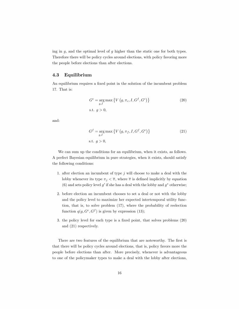
4.3 Equilibrium
An equilibrium requires a �xed point in the solution of the incumbent problem
17. That is:
Gc = argmaxg;I
�V�g; �c; I; G
f ; Gc�
(20)
s.t. g > 0,
and:
Gf = argmaxg;I
�V�g; �f ; I; G
f ; Gc�
(21)
s.t. g > 0,
We can sum up the conditions for an equilibrium, when it exists, as follows.
A perfect Bayesian equilibrium in pure strategies, when it exists, should satisfy
the following conditions:
1. after election an incumbent of type j will choose to make a deal with the
lobby whenever its type �j < �, where � is de�ned implicitly by equation
(6) and sets policy level g0 if she has a deal with the lobby and g� otherwise;
2. before election an incumbent chooses to set a deal or not with the lobby
and the policy level to maximize her expected intertemporal utility func-
tion, that is, to solve problem (17), where the probability of reelection
function q(g;Gc; Gf ) is given by expression (13);
3. the policy level for each type is a �xed point, that solves problems (20)
and (21) respectively.
There are two features of the equilibrium that are noteworthy. The �rst is
that there will be policy cycles around elections, that is, policy favors more the
people before elections than after. More precisely, whenever is advantageous
to one of the policymaker types to make a deal with the lobby after elections,
16

there will be electoral incentives that stimulate a higher policy for the poor
before election than after for each policymaker type.
The second feature is that a deal between the policymaker and the lobby is
more likely to happen after election than before. More speci�cally, whenever
an incumbent of a certain type makes a deal with the lobby before election,
she will also do it after election, but the converse is not true. A deal with the
lobby is pro�table for the incumbent only if the policy favors substantially this
group. However, elections induce the policymaker to set a policy more favorable
to the people, reducing the gain of an agreement with the lobby. Therefore an
agreement with the lobby is less likely before elections.
4.3.1 The possibility of no pure strategies equilibrium
Although it is plausible that a pure strategies equilibrium exists, there is no
guarantee. The model may not have an equilibrium if the type closer to the lobby
bene�ts marginally from a deal with the lobby after election. The argument is
outlined below.
Let the parameters be such that the policymaker of type �c opt for a contract
after election but for no contract before. As we will argue, this happens when
0 < �c � � < ", for a su¢ ciently small positive ", where � is the probability
cuto¤ level de�ned by equation (27). In this case the incumbent of type �cchooses to make a deal with the lobby after election and distorts policy. Thus,
FW (�j) > FU for both incumbent types, that is, they strictly prefer to be
reelected. For this reason, both incumbent types have an incentive to distort
policy to increase their reelection probability. Assume that, in equilibrium,
Gf > Gc, so that the reelection probability is increasing in g (by equation
(13)). The policymaker of type �c will face a con�ict of incentives between a
policy which leads to a higher probability of reelection - a higher g - and a policy
which will lead to higher personal bene�ts - a lower g. However, for a su¢ ciently
low " the deal with the lobby after elections is only marginally advantageous
to her, so that the additional electoral incentive makes a deal with the lobby
before election not advantageous. It is clear that the incumbent of type �f will
have even less incentives to set a deal with the lobby before elections, since
she faces a higher probability of a bad outcome. Hence, neither incumbent
types set a deal with the lobby before election. Their di¤erent incentives in
the pre-election policy choice comes from their di¤erent electoral incentives.
Since FW (�c)�FU > FW��f��FU , the policymaker of type �c will have a
17

higher reelection gain, therefore she will make a higher e¤ort to be reelected by
choosing a higher g. That is, Gf < Gc, which contradicts our initial assumption
that Gf > Gc.
An equilibrium with Gf < Gc is not possible either, since in this case the
probability function will be decreasing in g and the type �c will choose a lower
policy level. Then, the only remaining possibility is a pooling equilibrium, with
both types choosing policy level g�. However, this cannot be an optimal choice
for type �c, since in this case the incentives the policymaker faces before election
are the same she does after election, when she chooses to have a deal with the
lobby.
A speci�cation which leads to no equilibrium is not plausible in the context
of the present model. The model relies on the possibility of deals between the
policymaker and the lobby, and on non-observable comparative advantages of
certain types to bene�t from those deals. Thus, it is plausible to assume that
those deals bene�t substantially (not marginally) the type most attracted to
them - �c - under the most favorable conditions to them - after elections.
5 Applications
5.1 Government expenditure cycles
5.1.1 Expenditure composition cycles
There is evidence of electoral cycles for composition e¤ects on the �scal budget
in several countries (on US, see Peltzman 1992; on Canada, see Kneebone and
McKenzieon 2001; on Mexico, see Gonzalez 2004; on Colombia, see Drazen and
Eslava 2005). We now show how the framework developed above can be applied
to generate electoral expenditures composition cycles.
In the simple formulation we choose, taxes are �xed and there are two types
of public goods, speci�c to each of the two groups. The government budget
constraint is represented by:
� = (1� n) gl + ngp;
where � , gl and gp are taxes, expenditures for the lobby group and expenditures
for the people, respectively (all per capita). It can be rearranged as:
gl =� � ngp1� n :
18

A citizen of group i utility function ui is represented by:
ui (ci; gi) = ci + log gi, for i = p; l: � > 1;
where ci is her private consumption, gi is the amount of the public available to
her group, and p and l stand for the people and the lobby groups, respectively.
Given that ci = yi � � , indirect utility functions may be written as:
vl (g) = yl � � + log�� � ng1� n
�, and (22)
vp (g) = yp � � + log g; (23)
where we use g = gp for simplicity.
Substituting equations (22) and (23) into the utilitarian welfare function of
a benevolent policymaker, represented by equation (1), we get:
U (g) = y � � + n log g + (1� n) log�� � ng1� n
�; (24)
where y = nyp + (1� n) yl is the average per capita income. The benevolentpolicymaker would optimally choose:6
g� = � = gl; (25)
that is, all citizens would receive the same spending level.
The optimal spending level under a deal is given by:
g0 =�
1 + �b: (26)
Note that in this application we have an explicit solution for the spending level.
It is easy to check Proposition 1: g0 < g� and g0 is decreasing in �.
The cuto¤ probability � de�ned by equation (6) now becomes implicitly
de�ned by:
(1� n+ �b) log 1� n+ �b(1� n) � (1 + �b) log (1 + �b) = X (1� �) : (27)
Following the setup above, we are able to show that there will be an electoral
cycle in the expenditures composition, with more spending for the people before6Note that in this case it is economically reasonable to impose an upper bound for g
(0 < g � �n) to prevent a negative value for gl. However, this new restriction is never binding.
19

than after election. We provide a numerical example to illustrate the model�s
ability to generate electoral cycles.
Numerical example The Table 1 presents examples of the three possible
equilibrium types. The examples di¤er in the value of the loss X due to an
unsuccessful deal with lobby, while the other parameter values are set constant
at: �f = 0:25, �c = 0:75, n = 0:7, b = 0:5, � = 0:25, p = 0:5, and � = 0:9 .
The �rst line presents the results for a relatively small value for X, 0:01, which
makes a deal with the lobby always advantageous to both types before and after
elections. We observe that there is an expenditures cycle for both incumbent
types, with higher expenditures for the people before elections.Table 1: Expenditure Composition Electoral Cycle
X Gf
�Gc
�
Gf+1
�
Gc+1
� If Ic If+1 Ic+1
0.01 0.9219 0.8206 0.8889 0.7273 1 1 1 1
0.02 1.0237 0.8122 0.8889 0.7273 0 1 1 1
0.2 1.0195 0.7832 1 0.7273 0 1 0 1
Parameter values: n = 0:7; � = 0:9; b = 0:5; �f = 0:25; �c = 0:75; � = 0:25When we increase X to 0:02, we generate additionally a lobby activity elec-
toral cycle. Before the election, a deal with the lobby becomes not advantageous
to the type less connected with the lobby, despite being advantageous after elec-
tion. In order to increase her reelection probability, the policymaker of this type
prefers to increase her expenditure to a level above the optimal one, distorting
expenditure in a direction opposed to the lobby interests.
Increasing the damage of an unsuccessful deal further, to X = 0:2, will make
even an after election agreement with the lobby not bene�cial to the distant type
policymaker. However, the close type, having a higher probability of success in
the deal with the lobby, is still able to pro�t from the agreement, before and
after elections. We still have an expenditure cycle, with the close type choosing
to set a deal with the lobby before and after election, and the distant type not
setting the deal at any time.
Finally, an increase of X to the point that prevents any deal with the lobby
(not presented in the table) will result in an not very interesting type of equilib-
rium. Both types choose to spend � for both types of citizens, before and after
elections.
20

5.1.2 Aggregate expenditure cycles
Electoral cycles in aggregate expenditures can be generated by a simple change
in the model described above. Suppose that the people are not taxed and receive
the only public good.
vl (g) = yl � � , and (28)
vp (g) = yp + log g: (29)
We still assume a balance budget: g = � :
An utilitarian policymaker without lobby in�uence and electoral incentives
will choose:
g� =n
1� n:
If the policymaker chooses to spend g < g�, she can increase the lobby group
utility by g � g� and get a share B(g � g�). Then if she has a deal with thelobby, she would choose:
g0 =n
1� n+ �b =g�
1 + g��bn
; (30)
where, as before, b � [� � (1� n)]B.With information asymmetry about the two di¤erent policymaker types, �c
and �f , as before, the model generates electoral cycles in aggregate expenditures.
This result is in line with the empirical evidence, as in Brender and Drazen
(2004), Shi and Svensson (2002a,b), and Persson and Tabellini (2002).7
5.2 Exchange rate cycles
There is empirical evidence of exchange rate electoral cycles for Latin American
countries (cross-country evidence for Latin America is provided by Frieden,
Ghezzi and Stein, 2001, and Ghezzi, Stein and Streb, 2004, for Brazil, see
Bonomo and Terra, 2001, Grier and Hernández-Trillo, 2004 for Mexico, and
Pascó-Fonte and Ghezzi, 2001, for Peru). Bonomo and Terra (2005) presents
7Note that the balanced budget assumption also generates a counterfactual electoral taxcycle. In a more complex version of the model, we could assume, instead, that taxes are hard tochange and that any eventual budget imbalances could be �nanced by government debt. Thissetting would generate an intertemporally balanced budget equilibrium with expenditures andbudget de�cits electoral cycles.
21

a model that generates real exchange rate electoral cycles, in a setting with
informational asymmetry over the policymaker�s preferences. Here we derive the
same result in a simpler model based of the special interests politics proposed
in this paper.
Consider a endowment economy with two sectors: a tradable a nontradable
sector. The nontradable sector has the majority of the population, while the
tradable sector has the lobby power. All consumers are assumed to have the
same CES utility function:
u (Ni; Ti) =�N
r1+r
i + Tr
1+r
i
� 1+rr
; (31)
where Ni and Ti are the amount consumed of nontradable and tradable goods,
respectively, and r > 1. Now let e be the tradable good relative price, which is
the real exchange rate. De�ne g � 1e As expected, the indirect utility function
is decreasing in the real exchange rate for a citizen in the nontradable sector,
and increasing for the tradable sector:
vN (e) =�1 + g�r
�� 1r EN , and (32)
vT (e) = (1 + gr)� 1r ET ; (33)
where EN and ET are the per capita endowment for the nontradable and trad-
able sectors, respectively.
A benevolent (utilitarian) policymaker would choose to set the exchange rate
at a level8 :
g� =
�nEN
(1� n)ET
� 1r�1
(34)
The policymaker may choose to set a more depreciated exchange rate, g < g�
(which means e > e� � 1g� ) in order to favor the tradable sector and get a share
of its gain. Proceeding as before, we �nd that when there is an aggreement with
8We implicitly assume that the government manipulate its expenditure level in nontradablegoods to make the chosen exchange rate consistent with equilibrium in both nontradable andtradable goods markets. The government budget can be balanced intertemporally by a �xedlump sum tax on each citizen. Cyclical government budget imbalances are �nanced by foreinginvestors. For an example of a model where the relation between �scal policy and exchangerate is explicitly taken into account, see Bonomo and Terra (2004).
22

the tradable sector the chosen exchange rate is given by:
g0 =
�nEN
(1� n)ET + �bET
� 1r�1
(35)
= g��
1� n1� n+ �b
� 1r�1
(36)
By assuming that there are two types of policymakers, �c and �f , informa-
tion asymmetry engenders a mechanism by which exchange rate electoral cycles
are generated. The policymaker will choose a more appreciated exchange rate
before than after election.
6 Conclusion
Special interest politics is often associated with microeconomic policy, and its
macroeconomic impact is thought to be negligible. Here we are concerned with
opposite interests which divide the entire society in two groups: one with the
lobby power, and the other with the majority of votes. Government policy may
a¤ect the distribution of resources in the society between those two groups.
In this paper we propose a link between special interest politics and political
business cycles. We build a framework where the lobby power of a special
interest group interacts with the voting power of the majority of the population,
leading to political business cycles. The model generates an additional cycle,
which is a �contracting�cycle around elections. Since reelection concerns induce
the policymaker to favor less the lobby group, the mutual net gains from a deal
between the incumbent and the lobby are reduced before elections. Therefore, it
is less likely that the policymaker will make a deal with the lobby group before
elections than after elections.
We showed that those same ideas could be applied to generate cycles around
election in other economic variables, such as government expenditures level, and
the real exchange rate.
The mechanism we propose in this paper does not exclude the operation of
traditional political business cycle channels, as proposed by the opportunistic
and partisan literature. The relative importance of our proposed channel in
explaining the electoral cycle in di¤erent variables should be investigated in
future research.
23
References
[1] Alesina, A. (1987), Macroeconomic Policy in a Two-Party System as a
Repeated Game. Quarterly Journal of Economics 102, 651-78.
[2] Bonomo, M. and C. Terra (2005). �Elections and Exchange Rate Policy
Cycles,�Economics and Politics, forthcoming.
[3] Bonomo, M. and C. Terra (2001), The Dilemma of In�ation vs Balance of
Payments: Crawling Pegs in Brazil, 1964-98, in: J. Frieden and E. Stein,
eds., The Currency Game: Exchange Rate Politics in Latin America (IDB,
Washington).
[4] Brender, A. and A. Drazen (2004), "Political Budget Cycles in New Versus
Established Democracies," NBER Working Paper 10539.
[5] Cukierman, A. and A.Meltzer (1986), A Positive Theory of Discretionary
Policy, the Costs of Democratic Government, and the Bene�ts of a Consti-
tution. Economic Inquiry 24, 367-88.
[6] Downs, Anthony (1957). An Economic Theory of Democracy, Addison Wes-
ley.
[7] Drazen, A. and M. Eslava (2005a), "Electoral Manipulation via Expendi-
ture Composition: Theory and Evidence," NBER Working Paper 11085.
[8] Drazen, A. and M. Eslava (2005b), "Political Budget Cycles When Politi-
cians Have Favorites," mimeo, University of Maryland.
[9] Frieden, J. and E. Stein (2001), The Currency Game: Exchange Rate Pol-
itics in Latin America, IDB, Washington.
[10] Frieden, J., P. Ghezzi and E. Stein (2001), Politics and Exchange Rates:
A Cross Country Study, in: J. Frieden and E. Stein, eds., The Currency
Game: Exchange Rate Politics in Latin America (IDB, Washington).
[11] Ghezzi, P., E. Stein and J. Streb (2004), �Real Exchange Rate Cycles
around Elections,�Economics and Politics, forthcoming.
[12] Gonzalez, Maria de los A. (2004), �Do Changes in Democracy A¤ect the
Political Budget Cycle?,�Review of Development Economics, forthcoming.
24

[13] Grier, Kevin B. and Fausto Hernández-Trillo (2004), �The Real Exchange
Rate Process and Its Real E¤ects,�Journal of Applied Economics VII(1):
1-25
[14] Grossman, Gene and Elhanan Helpman (1994), �Protection for Sale,�
American Economic Review 84: 833-50.
[15] Grossman, Gene and Elhanan Helpman (1996), �Electoral Competition and
Special Interest Politics,�Review of Economic Studies 63: 265-286.
[16] Grossman, Gene and Elhanan Helpman (2001), Special Interest Politics,
MIT Press.
[17] Hibbs, D. (1977), Political Parties and Macroeconomic Policy. American
Political Science Review 71, 146-87.
[18] Holmstrom, Bengt (1999), �Managerial Incentive Problems: A Dynamic
Perspective,�Review of Economic Studies 66: 169-182.
[19] Kneebone, R. and K. McKenzie (2001), �Electoral and Partisan Cycles in
Fiscal Policy: an Examination of Canadian Provinces,� International Tax
and Public Finance 8: 753-774.
[20] Lindbeck, A. (1976), Stabilization Policies in Open Economies with En-
dogenous Politicians. American Economic Review Papers and Proceedings,
1-19.
[21] Nordhaus, W. (1975), The Political Business Cycle. Review of Economic
Studies 42, 169-90.
[22] Pascó-Fonte, A. and P. Ghezzi (2001), Exchange Rates and Interest Groups
in Peru, 1950-1996, in: J. Frieden and E. Stein, eds., The Currency Game:
Exchange Rate Politics in Latin America (IDB, Washington).
[23] Peltzman, S. (1992), "Voters as Fiscal Conservatives," Quarterly Journal
of Economics 107, 327-361.
[24] Persson, T. and G.Tabellini (2000), Political Economics: Explaining Eco-
nomic Policy (The MIT Press).
[25] Persson, T. and G. Tabellini (2002), "Do Electoral Cycles Di¤er Across
Political Systems?" working paper.
25
[26] Rogo¤, K. (1990), �Equilibrium Political Budget Cycles,�American Eco-
nomic Review 80: 21-36.
[27] Rogo¤, K. and A. Silbert (1988), �Elections and Macroeconomic Policy
Cycles,�Review of Economic Studies 55: 1-16.
[28] Shi, E. and J. Svensson (2002a), "Conditional Political Business Cycles,"
CEPR Discussion Paper #3352.
[29] Shi, E. and J. Svensson (2002b), �Political Business Cycles in Developed
and Developing Countries,�mimeo.
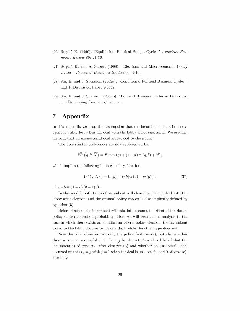
7 Appendix
In this appendix we drop the assumption that the incumbent incurs in an ex-
ogenous utility loss when her deal with the lobby is not successful. We assume,
instead, that an unsuccessful deal is revealed to the public.
The policymaker preferences are now represented by:
fW 0�g;ec; eX� = E [nvp (g) + (1� n) vl (g;ec) + �ec] ;
which implies the following indirect utility function:
W 0 (g; I; �) = U (g) + I�b [vl (g)� vl (g�)] , (37)
where b � (1� n) (� � 1)B.In this model, both types of incumbent will choose to make a deal with the
lobby after election, and the optimal policy chosen is also implicitly de�ned by
equation (5).
Before election, the incumbent will take into account the e¤ect of the chosen
policy on her reelection probability. Here we will restrict our analysis to the
case in which there exists an equilibrium where, before election, the incumbent
closer to the lobby chooses to make a deal, while the other type does not.
Now the voter observes, not only the policy (with noise), but also whether
there was an unsuccessful deal. Let �j be the voter�s updated belief that the
incumbent is of type �f , after observing bg and whether an unsucessful dealoccurred or not (Ix = j with j = 1 when the deal is unsucessful and 0 otherwise).
Formally:
26

�j = Pr (�t = �f jbgt = bg; Ix = j )If an unsucessful deal occurs, the voter will infer that the policymaker type
is �f . Therefore �1 = 0. In this case the incumbent will not be reelected.
The updated belief when the voter receives no signal of an unsuccessful deal
is:
�0 =p� h(bgt = bg; Ix = 0 j�t = �f )
p� h(bgt = bg; Ix = 0 j�t = �f ) + (1� p)� h(bgt = bg; Ix = 0 j�t = �c ) ;(38)
where h(bgt = bg; Ix = 0 j�t = �i ) is the joint density of observing a policy signal bgand receiving no information about an unsucessful deal, given the the incumbent
type is �i.
It is clear that:
h (bgt = bg; Ix = 0 j�t = �c ) = �c � f (bgt = bg j�t = �c ) ; and (39)
h (bgt = bg; Ix = 0 j�t = �f ) = f (bgt = bg j�t = �f ) ;since the sucess of the deal is assumed to be independent of the policy chosen
by the incumbent when the incumbent makes a deal with the lobby.
When the voters receive no information about an unsucessful deal, the in-
cumbent will be reelected if �0 > p, which, after substituing equation (39) into
(38), can be seen to be equivalent to:
f (bgt = bg j�t = �f ) > �c � f (bgt = bg j�t = �c ) :Given the assumed lognormal distribution for the noise, the cuto¤ for the
observed policy signal eg will be given by:ln eg = lnGf + lnGc
2+
ln�clnGf � lnGc
The reelection probability for an incumbent which chooses a policy g and
whether to set a deal I can easily be shown to be given by:
q0�g; I;Gf ; Gc
�= [1� I (1� �i)]
�1� �
�ln eg � ln g
�
��. (40)
Note that the reelection probability decreases when the incumbent chooses
27

to make a deal with the lobby.
The intertemporal utility function of the incumbent becomes:
V 0�g; I; �i; G
f ; Gc�= (41)
W 0(g; I; �i) + �q0 �g; I;Gf ; Gc� [FW (�i)� FU ] + �FU:
Observe that, when I = 0; V 0 (:) becomes the same function as in the original
problem. However, this does not mean that Gf will be the same as before, since
it depends on Gc. The closer type faces a di¤erent objective function, as the
reelection probability is a di¤erent function of g.
28