Special Topics in Complexity Theory

Emanuele Viola

December 28, 2017

This document collects the Fall 2017 lectures given by the instructor.Compared to the lectures on the class website, I have made some minor editsto harmonize the various lectures. In addition we had two guest lecturesand presentations by students, which can also be found on the class website.Many thanks to Matthew Dippel, Xuangui Huang, Chin Ho Lee, BiswaroopMaiti, Tanay Mehta, Willy Quach, and Giorgos Zirdelis for doing an excellentjob scribing these lectures. Many thanks also to all the students, postdocs,and faculty who attended the class and created a great atmosphere.

Contents

1 Bounded independence 31.1 Background . . . . . . . . . . . . . . . . . . . . . . . . . . . . 31.2 k-wise independent distribution . . . . . . . . . . . . . . . . . 41.3 Lower bounds . . . . . . . . . . . . . . . . . . . . . . . . . . . 61.4 Who is fooled by k-wise independence? . . . . . . . . . . . . . 7

1.4.1 k-wise independence fools AND . . . . . . . . . . . . . 71.5 Bounded Independence Fools AC0 . . . . . . . . . . . . . . . . 12

1.5.1 Approximation 1 . . . . . . . . . . . . . . . . . . . . . 131.6 Approximation 2 . . . . . . . . . . . . . . . . . . . . . . . . . 141.7 Bounded Independence Fools AC0 . . . . . . . . . . . . . . . . 15

2 Small-bias distributions 182.1 Constructions of small bias distributions . . . . . . . . . . . . 192.2 An improved small bias distribution via bootstrapping . . . . 202.3 Connecting small bias to k-wise independence . . . . . . . . . 21

1

2.4 Fourier analysis of boolean functions 101 . . . . . . . . . . . . 212.5 Small bias distributions are close to k-wise independent . . . . 222.6 An improved construction . . . . . . . . . . . . . . . . . . . . 24

3 Tribes Functions and the GMRTV Generator 24

4 Bounded indistinguishability 284.1 Duality. . . . . . . . . . . . . . . . . . . . . . . . . . . . . . . 294.2 Approximate Degree of AND. . . . . . . . . . . . . . . . . . . 334.3 Approximate Degree of AND-OR. . . . . . . . . . . . . . . . . 354.4 Lower Bound of d1/3(AND-OR) . . . . . . . . . . . . . . . . . 364.5 Lower Bound of d1/3(SURJ) . . . . . . . . . . . . . . . . . . . 38

5 Pseudorandom groups and communication complexity 415.1 2-party communication protocols . . . . . . . . . . . . . . . . 445.2 3-party communication protocols . . . . . . . . . . . . . . . . 445.3 A randomized protocol for the hypercube . . . . . . . . . . . . 445.4 A randomized protocol for Zm . . . . . . . . . . . . . . . . . . 455.5 Other groups . . . . . . . . . . . . . . . . . . . . . . . . . . . 465.6 More on 2-party protocols . . . . . . . . . . . . . . . . . . . . 49

6 Number-on-forehead communication complexity 51

7 Corners in pseudorandom groups 527.1 Proof Overview . . . . . . . . . . . . . . . . . . . . . . . . . . 537.2 Weak Regularity Lemma . . . . . . . . . . . . . . . . . . . . . 547.3 Getting more for rectangles . . . . . . . . . . . . . . . . . . . 557.4 Proof . . . . . . . . . . . . . . . . . . . . . . . . . . . . . . . . 56

7.4.1 Parameters . . . . . . . . . . . . . . . . . . . . . . . . 59

8 Static data structures 59

2

1 Bounded independence

In this first lecture we begin with some background on pseudorandomnessand then we move on to the study of bounded independence, presenting inparticular constructions and lower bounds.

1.1 Background

Let us first give some background on randomness. There are 3 differenttheories:

(1) Classical probability theory. For example, if we toss a coin 12 timesthen the probability of each outcome is the same, i.e., Pr[010101010101] =Pr[011011100011]. However, intuitively we feel that the first outcome is lessrandom than the second.

(2) Kolmogorov complexity. Here the randomness is measured by thelength of the shortest program outputting a string. In the previous example,the program for the second outcome could be “print 011011100011”, whereasthe program for the first outcome can be “print 01 six times”, which is shorterthan the first program.

(3) Pseudorandomness. This is similar to resource-bounded Kolmogorovcomplexity. Here random means the distribution “looks random” to “efficientobservers.”

Let us now make the above intuition precise.

Definition 1.[Pseudorandom generator (PRG)] A function f : 0, 1s →0, 1n is a pseudorandom generator (PRG) against a class of tests T ⊆t : 0, 1n → 0, 1 with error ε, if it satisfies the following 3 conditions:

(1) the output of the generator must be longer than its input, i.e., n > s;(2) it should fool T , that is, for every test t ∈ T , we have Pr[t(Un) = 1] =

Pr[t(f(Us)) = 1]± ε;(3) the generator must be efficient.

To get a sense of the definition, note that a PRG is easy to obtain if wedrop any one of the above 3 conditions. Dropping condition (1), then we candefine our PRG as f(x) := x. Dropping condition (2), then we can define ourPRG as f(x) := 0. Dropping condition (3), then the PRG is not as obviousto obtain as the previous two cases. We have the following claim.

Claim 2. For every class of tests T , there exists an inefficient PRG witherror ε and seed length s = lg2 lg2(|T |) + 2 lg2(1/ε) +O(1).

3

Before proving the claim, consider the example where T is the class ofcircuits of size n100 over n-bit input, it is known that |T | = 2n

O(1). Hence,

applying our claim above we see that there is an inefficient PRG that foolsT with error ε and seed length s = O(lg2(n/ε)).

We now prove the claim using the probabilistic method.

Proof. Consider picking f at random. Then by the Chernoff bound, we havefor every test t ∈ T ,

Prf

[|PrUs

[t(f(Us)) = 1]− PrUn

[t(Un) = 1]| ≥ ε] ≤ 2−Ω(ε22s) < 1/|T |,

if s = lg2 lg2(|T |)+2 lg2(1/ε)+O(1). Therefore, by a union bound over t ∈ T ,there exists a fixed f such that for every t ∈ T , the probabilities are withinε.

1.2 k-wise independent distribution

A major goal in research in pseudorandomness is to construct PRGs for (1)richer and richer class T , (2) smaller and smaller seed length s, and makingthe PRG explicit. For starters, let us consider a simple class of tests.

Definition 3.[d-local tests] The d-local tests are tests that depend only on dbits.

We will show that for this class of tests we can actually achieve errorε = 0. To warm up, consider what happens when d = 1, then we can have aPRG with seed length s = 1 by defining f(0) := 0n and f(1) := 1n.

For d = 2, we have the following construction. Define

f(x)y := 〈x, y〉 =∑i

xiyi mod 2.

Here the length of x and y is |x| = |y| = lg2 n, and we exclude y = 0lg2 n.Note that the output has n− 1 bits, but we can append one uniform bit tothe output of f . So the seed length would be lg2 n+ 1.

Now we prove the correctness of this PRG.

Claim 4. The f defined above is a PRG against 2-local tests with errorε = 0.

4

Proof. We need to show that for every y 6= z, the random variable (f(x)y, f(x)z)over the choice of x is identical to U2, the uniform 2-bit string. Since y 6= z,suppose without loss of generality that there exists an i such that yi = 1 andzi = 0. Now f(x)z is uniform, and conditioned on z, f(x)y is also uniform,thanks to the index yi.

The case for d = 3 becomes much more complicated and involves the useof finite fields. One can think of a finite field as a finite domain that behaveslike Q in the sense that it allows you to perform arithmetic operations, in-cluding division, on the elements. We will use the following fact about finitefields.

Lemma 5. There exist finite fields of size pk, for every prime p and integerk. Moreover, they can be constructed and operated with in time poly(k, p).

Remark 6. Ideally one would like the dependence on p to be lg2 p. However,such construction remains an open question and there have been many at-tempts to constructing finite fields in time poly(k, lg2 p). Here we only workwith finite fields with p = 2, and there are a lot of explicit constructions forthat.

One simple example of finite fields are integers modulo p.

Theorem 7. Let D = 0, 1lg2 n. For every k, there exists an explicitconstruction over Dn such that

(1) elements in Dn can be sampled with s = k lg2 n bits, and(2) every k symbols are uniform in Dk.

For d = 3, we can use the above theorem with k = 3, and the PRG canoutput the first bit of every symbol.

Remark 8. There exist other constructions that are similar to the innerproduct construction for the case d = 2, with y carefully chosen, but the wayto choose y involves the use of finite fields as well.

Note that we can also apply the theorem for larger d to fool d-local testswith seed length s = d lg2 n.

We now prove the theorem.

Proof. Pick a finite field F of size 2lg2 n. Let a0, . . . , an−1 ∈ F be uniformrandom elements in F which we think of as a polynomial a(x) of degree

5

k − 1. We define the generator f to be

f(a0, . . . , an−1)x = a(x) =n−1∑i=0

aixi.

(One should think of the outputs of f as lines and curves in the real plane.)The analysis of the PRG follows from the following useful fact: For every

k points (x0, y0), (x1, y1), . . . , (xk−1, yk−1), there exists exactly one degree k−1polynomial going through them.

Let us now introduce a terminology for PRGs that fool d-local tests.

Definition 9. We call distributions that look uniform (with error 0) to k-local tests k-wise independent (also known as k-wise uniform). The latterterminology is more precise, but the former is more widespread.

We will soon see an example of a distribution where every k elements areindependent but not necessarily uniform.

1.3 Lower bounds

We have just seen a construction of k-wise independent distributions withseed length s = d lg2 n. It is natural to ask, what is the minimum seed lengthof generating k-wise independent distributions?

Claim 10. For every k ≥ 2, every PRG for k-local tests over 0, 1n hasseed length s ≥ Ω(k lg2(n/k)).

Proof. We use the linear-algebraic method. See the book by Babai–Frankl [BF92]for more applications of this method.

To begin, we will switch from 0, 1 to −1, 1, and write the PRG as a2s × n matrix M , where the rows are all the possible outputs of the PRG.Since the PRG fools k-local tests and k ≥ 2, one can verify that every 2columns of M are orthogonal, i.e., 〈Mi,Mj〉 = 0 for i 6= j. As shown below,this implies that the vectors are independent. And by linear algebra thisgives a lower bound on s.

However so far we have not used k. Here’s how to use it. Consider allthe column vectors v obtained by taking the entry-wise products of any ofthe k/2 vectors in M . Because of k-wise independence, these v’s are againorthogonal, and this also implies that they are linearly independent.

6

Claim 11. If v1, v2, . . . , vt are orthogonal, then they are linearly independent.

Proof. Suppose they are not and we can write vi =∑

j∈S,i6∈S vj for someS. Taking inner product with vi on both sides, we have that the L.H.S. isnonzero, whereas the R.H.S. is zero because the vectors are orthogonal, acontradiction.

Therefore, the rank of M must be at least the number of v’s, and so

2s ≥ number of v’s ≥(n

k/2

)≥ (2n/k)k/2.

Rearranging gives s ≥ (k/2) lg2(2n/k).

1.4 Who is fooled by k-wise independence?

In the coming lectures we will see that k-wise independence fools AC0, theclass of constant-depth circuits with unbounded fan-in. Today, let us seewhat else is fooled by k-independence in addition to k-local tests.

(1) Suppose we have n independent variables x1, . . . , Xn ∈ [0, 1] and wewant to understand the behavior of their sum

∑iXi. Then we can apply

tools such as the Chernoff bound, tail bounds, Central Limit Theorem, andthe Berry–Esseen theorem. The first two give bounds on large deviation fromthe mean. The latter two are somewhat more precise facts that show thatthe sum will approach a normal distribution (i.e., the probability of beinglarger than t for any t is about the same). One can show that similar resultshold when the Xi’s are k-wise independent. The upshot is that the Chernoffbound gives error 2−samples, while under k-wise independence we can only getan error (samples)−k/2.

(2) We will see next time that k-wise independence fools DNF and AC0.(3) k-wise independence is also used as hashing in load-balancing.

1.4.1 k-wise independence fools AND

We now show that k-wise independent distributions fool the AND function.

Claim 12. Every k-wise uniform distribution fools the AND functions onbits with error ε = 2−Ω(k).

7

Proof. If the AND function is on at most k bits, then by definition the erroris ε = 0. Otherwise the AND is over more than k bits. Without loss ofgenerality we can assume the AND is on the first t > k bits. Observe thatfor any distribution D, we have

PrD

[AND on t bits is 1] ≤ PrD

[AND on k bits is 1].

The right-hand-side is the same under uniform and k-wise uniformity, and is2−k. Hence,

| Pruniform

[AND = 1]− Prk-wise ind.

[AND = 1]| ≤ 2−k.

Instead of working over bits, let us now consider what happens over ageneral domain D. Given n functions f1, . . . , fn : D → 0, 1. Supposex1, . . . , xn are k-wise uniform over Dn. What can you say about the AND ofthe outputs of the fi’s, f1(x1), f2(x2), . . . , fn(xn)?

This is similar to the previous example, except now that the variables areindependent but not necessarily uniform. Nevertheless, we can show that asimilar bound of 2−Ω(k) still holds.

Theorem 13.[[EGL+92]] LetX1, X2, . . . , Xn be random variables over 0, 1,which are k-wise independent, but not necessarily uniform. Then

Pr[n∏i=1

Xi = 1] =n∏i=1

Pr[Xi = 1]± 2−Ω(k).

This fundamental theorem appeared in the conference version of [EGL+92],but was removed in the journal version. One of a few cases where the journalversion contains less results than the conference version.

Proof. Let D be the distribution of (X1, . . . , Xn). Let B be the n-wise in-dependent distribution (Y1, . . . , Yn) such that Pr[Yi = 1] = Pr[Xi = 1] forall i ∈ [n] and the Yi are independent. The theorem is equivalent to thefollowing statement.

| PrX←D

[n∧i=1

Xi = 1

]− Pr

X←B

[n∧i=1

Xi = 1

]| ≤ 2−Ω(k)

8

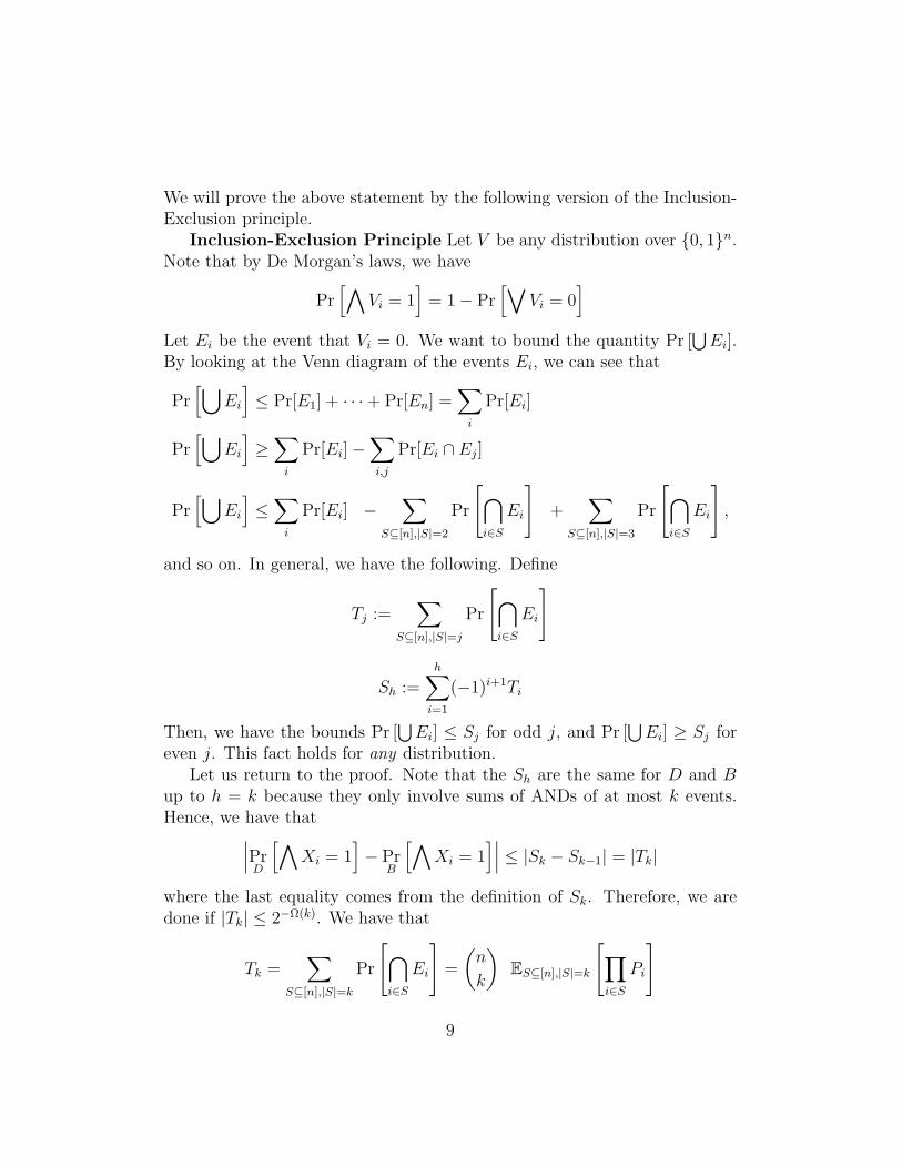
We will prove the above statement by the following version of the Inclusion-Exclusion principle.

Inclusion-Exclusion Principle Let V be any distribution over 0, 1n.Note that by De Morgan’s laws, we have

Pr[∧

Vi = 1]

= 1− Pr[∨

Vi = 0]

Let Ei be the event that Vi = 0. We want to bound the quantity Pr [⋃Ei].

By looking at the Venn diagram of the events Ei, we can see that

Pr[⋃

Ei

]≤ Pr[E1] + · · ·+ Pr[En] =

∑i

Pr[Ei]

Pr[⋃

Ei

]≥∑i

Pr[Ei]−∑i,j

Pr[Ei ∩ Ej]

Pr[⋃

Ei

]≤∑i

Pr[Ei] −∑

S⊆[n],|S|=2

Pr

[⋂i∈S

Ei

]+

∑S⊆[n],|S|=3

Pr

[⋂i∈S

Ei

],

and so on. In general, we have the following. Define

Tj :=∑

S⊆[n],|S|=j

Pr

[⋂i∈S

Ei

]

Sh :=h∑i=1

(−1)i+1Ti

Then, we have the bounds Pr [⋃Ei] ≤ Sj for odd j, and Pr [

⋃Ei] ≥ Sj for

even j. This fact holds for any distribution.Let us return to the proof. Note that the Sh are the same for D and B

up to h = k because they only involve sums of ANDs of at most k events.Hence, we have that∣∣∣Pr

D

[∧Xi = 1

]− Pr

B

[∧Xi = 1

]∣∣∣ ≤ |Sk − Sk−1| = |Tk|

where the last equality comes from the definition of Sk. Therefore, we aredone if |Tk| ≤ 2−Ω(k). We have that

Tk =∑

S⊆[n],|S|=k

Pr

[⋂i∈S

Ei

]=

(n

k

)ES⊆[n],|S|=k

[∏i∈S

Pi

]

9

where Pi := Pr[Ei] = 1 − Pr[Xi = 1]. To bound the expectation we recall auseful inequality.

A Useful Inequality Let Q1, . . . , Qn be non-negative real numbers.Then, by the AM-GM inequality, we have that∑

iQi

n≥

(∏i

Qi

)1/n

.

Consider the following more general statement,

ES⊆[n],|S|=1

[∏i∈S

Qi

]≥ ES⊆[n],|S|=2

[∏i∈S

Qi

]1/2

≥ . . .

· · · ≥ ES⊆[n],|S|=k

[∏i∈S

Qi

]1/k

≥ · · · ≥ ES⊆[n],|S|=n

[∏i∈S

Qi

]1/n

and note that the left most term is equal to∑

i Qi

n, while the right most term

is equal to (∏

iQi)1/n

Applying the above inequality to Tk and a common approximation for thebinomial coefficient, we have that

Tk =

(n

k

)ES⊆[n],|S|=k

[∏i∈S

Pi

]≤(n

k

) n∑i=1

(Pin

)k≤(enk

)k (∑Pin

)k=

(e∑Pi

k

)k.

Therefore, we are done if∑Pi ≤ k

2e. Recall that Pi = Pr[Ei] = 1 −

Pr[Xi = 1]. So if Pi is small then Pr[Xi = 1] is close to 1.It remains to handle the case that

∑Pi ≥ k

2e. Pick n′ such that

n′∑i=1

Pi =k

2e± 1.

By the previous argument, the AND of the first n′ is the same up to 2−Ω(k)

for D and B. Also, for every distribution the probability of that the And ofn bits is 1 is at most the probability that the And of n′ bits is 1. And also,

10

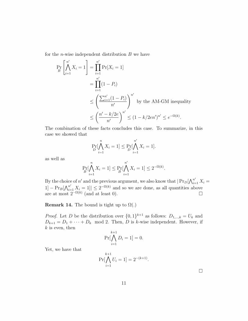
for the n-wise independent distribution B we have

PrB

[n′∧i=1

Xi = 1

]=

n′∏i=1

Pr[Xi = 1]

=n′∏i=1

(1− Pi)

≤

(∑n′

i=1(1− Pi)n′

)n′

by the AM-GM inequality

≤(n′ − k/2e

n′

)n′≤ (1− k/2en′)n′ ≤ e−Ω(k).

The combination of these facts concludes this case. To summarize, in thiscase we showed that

PrD

[n∧i=1

Xi = 1] ≤ PrD

[n′∧i=1

Xi = 1].

as well as

PrB

[n∧i=1

Xi = 1] ≤ PrB

[n′∧i=1

Xi = 1] ≤ 2−Ω(k).

By the choice of n′ and the previous argument, we also know that |PrD[∧n′

i=1Xi =

1] − PrB[∧n′

i=1 Xi = 1]| ≤ 2−Ω(k) and so we are done, as all quantities aboveare at most 2−Ω(k) (and at least 0).

Remark 14. The bound is tight up to Ω(.)

Proof. Let D be the distribution over 0, 1k+1 as follows: D1,...,k = Uk andDk+1 = D1 + · · · + Dk mod 2. Then, D is k-wise independent. However, ifk is even, then

Pr[k+1∧i=1

Di = 1] = 0.

Yet, we have that

Pr[k+1∧i=1

Ui = 1] = 2−(k+1).

11

1.5 Bounded Independence Fools AC0

Acknowledgement. This section is based on Amnon Ta-Shma’s notes forthe class 0368.4159 Expanders, Pseudorandomness and Derandomization CSdept, Tel-Aviv University, Fall 2016.

Note that a DNF on n bits can be modeled as a depth two circuit wherethe top layer is an OR-gate whose inputs are AND-gates, which take inputsX1, . . . , Xn and their negations. The circuit class AC0 can be viewed asa generalization of this to higher (but constant) depth circuits. That is,AC0 consists of circuits using AND-gates, OR-gates, NOT-gates, and inputregisters. Each of the gates have unbounded fan-in (i.e. the number of inputwires). The size of the circuit is defined to be the number of gates.

AC0 is one of the most studied classes in complexity theory. AC0 circuitsof polynomial size can do many things, including adding and subtractingn-bit integers.

Conjecture 15.[Linial-Nisan[LN90]] logO(d) s-wise independence fools AC0

circuits of depth d and size s.

The conjecture was open for a long time, even for in the special case d = 2.In 2007 a breakthrough work by Bazzi [Baz09] proved it for d = 2. Shortlyafterwards, Razborov presented a simpler proof of Bazzi’s result [Raz09], and

Braverman proved the conjecture for any d with logd2

s-wise independence[Bra10]. Tal improved the result to logO(d) s [Tal17].

Interestingly, the progress on the conjecture does not use ideas that werenot around since the time of its formulation. Bottom line: if a problem isopen for a long time, you should immediately attack it with existing tools.

The high-level intuition why such a result should be true is the following:

1. AC0 is approximated by polylog degree polynomials.

2. k-wise independence fools degree-k polynomials.

Proof of (2). Let x = (x1, . . . , xn) ∈ 0, 1n. Let p(x1, . . . , xn) be a degree kpolynomial over R. Write p as

p(x1, . . . , xn) =∑

M⊆[n],|M |≤k

cM · xM .

12

If D is a k-wise independent distribution on 0, 1n, then by linearity ofexpectation

ED[P ] =∑

M⊆[n],|M |≤k

cMED[xM ] =∑

M⊆[n],|M |≤k

cMEU [xM ] = EU [P ].

There are several notions of approximating AC0 by low-degree polynomi-als. We now review two of them, explaining why neither of them is sufficient.Braverman showed how to cleverly combine the two methods to prove a ver-sion of (1) that’s strong enough.

1.5.1 Approximation 1

Theorem 16. For all AC0 circuits C(x1, . . . , xn) of size s and depth d, for alldistributions D over 0, 1n, for all ε, there exists a polynomial p(x1, . . . , xn)of degree logO(d) s/ε such that

Prx←D

[p(x) = C(x)] ≥ 1− ε.

The important features of this approximation are that it works under anydistribution, and when the polynomial is correct it outputs a boolean value.

Similar approximations appear in many papers, going back to Razborov’spaper [Raz87] (who considers polynomials modulo 2) which uses ideas fromearlier still work.

Note that the polynomial p depends on the circuit C chosen, and on thedistribution. This theorem is not a good enough approximation because onthe ε fraction of inputs where the polynomial and circuit are unequal, thevalue of the polynomial can (and does) explode to be much greater than 1/ε.This prevents us from bounding the average of the polynomial.

Nevertheless, let us prove the above theorem.

Proof. Consider one OR-gate of fan-in s. We construct a distribution ofpolynomials that compute any input with high probability. This impliesthat there is a fixed polynomial that computes the circuit on a large fractionof the inputs by an averaging argument.

13

For i = 1, 2, . . . , log s. let Si be a random subset of [s] where every elementis included with probability 1/2i, independently.

Suppose x has Hamming weight 2j. Then, E[∑

n∈Sjxn] = 1. And the

sum can be shown to equal 1 with constant probability.Define the approximation polynomial p to be

p(x) := 1−log s∏i=1

(1−∑h∈Si

xh)

Note that if x has weight w > 0, then p(x) = 0 with constant probability. Ifw = 0, then p(x) = 1 with probability 1. We can adjust the error probabilityto ε by repeating each term in the product log(1/ε) times.

Thus, we can approximate one gate with the above polynomial of degreeO(log(s) · log(1/ε)). Construct polynomials as p above for each gate, witherror parameter ε/s. The probability that any of them is wrong is at mostε by a union bound. To obtain the approximating polynomial for the wholecircuit compose all the polynomials together. Since the circuit is of depthd, the final degree of the approximating polynomial is (log(s) · log(s/ε))d, asdesired.

As mentioned at the beginning, this is a distribution on polynomials thatcomputes correctly any input with probability at least 1 − ε. By averaging,there exists a fixed polynomial that computes correctly a 1 − ε fraction ofinputs.

It can be verified that the value of the polynomial can be larger than 1/ε.The polynomial for the gates closest to the input can be as large as s. Thenat the next level it can be as large as slog s/ε, which is already much largerthan 1/ε.

1.6 Approximation 2

Theorem 17. For all circuits C of size s and depth d, for all error values ε,there exists a polynomial p(x1, . . . , xn) of degree O(log(s)d−1 log(1/ε)) suchthat

Ex←Un [(C(x)− p(x))2] ≤ ε.

14

The important feature of this approximation is that it bounds the average,but only under the uniform distribution. Because it does not provide anyguarantee on other distributions, including k-wise independent distributions,it cannot be used directly for our aims.

Remark 18. Approximation 2 is proved via the switching lemma, an in-fluential lemma first proved in the early 80’s by Ajtai [Ajt83] and by Furst,Saxe, and Sipser [FSS84]. The idea is to randomly set a subset of the vari-ables to simplify the circuit. You can do this repeatedly to simplify thecircuit even further, but it only works on the uniform distribution. Hastad[Has87] gave a much tighter analysis of the switching lemma, and the paper[LMN93] used it to prove a version of Approximation 2 with a slightly worsedependence on the error. Recently, a refinement of the switching lemma wasproved in [Has14, IMP12]. Based on that, Tal [Tal17] obtained the corre-sponding refinement of Approximation 2 where the parameters are as statedabove. (The polynomial is simply obtained from the Fourier expansion of thefunction computed by the circuit by removing all Fourier coefficients largerthan a certain threshold. The bound on the Fourier decay in [Tal17] impliesthe desired approximation.)

1.7 Bounded Independence Fools AC0

Theorem 19. For all circuits C with unbounded fan-in of size s and depthd, for all error values ε, for all k-wise independent distributions D on 0, 1n,we have that

|E[C(D)]− E[C(Un)]| ≤ ε

for k = log(s/ε)O(d).

Corollary 20. In particular, if s = poly(n), d = O(1), s = 1/poly(n), thenk = logO(1)(n) suffices.

The next claim is the ultimate polynomial approximation used to provethe theorem.

Claim 21. For all circuits C with unbounded fan-in of size s and depth d,for all error values ε, for all k-wise independent distributions D on 0, 1n,there is a set E of inputs, and a degree-k polynomial p such that:

1. E is ’rare’ under both D and Un:

15

Prx←Un [E(x) = 1] ≤ ε, and Prx←D[E(x) = 1] ≤ ε. Here we write E(x)for the indicator function of the event x ∈ E.

2. For all x, p(x) ≤ C(x) ∨ E(x). Here ∨ is the logical Or.

3. E[p(Un)] = E[C(Un)]± ε.

We only need (1) under D, but (1) under U is used to prove (3).

Proof of Theorem 19 from Claim 21.

E[C(D)] = E[C(D) ∨ E(D)]± ε, by Claim.(1)

≥ E[p(D)]± ε, by Claim.(2)

= E[p(Un)]± ε, because p has degree k and D is k-wise independent

= E[C(Un)]± ε, by Claim.(3)

For the other direction, repeat the argument for ‘not C’.

We can construct the polynomial approximation from Claim 21 by us-ing a combination of Approximation 1 and 2. First we need a little moreinformation about Approximation 1.

Claim 22. Two properties of approximation 1:

1. For all x, p(x) ≤ 2log(s/ε)O(d).

2. The ’bad’ set E is computable by a circuit of size poly(s), and depthd+O(1).

Proof of Claim 22 part 2. Consider a single OR gate with input gates g1, . . . , gs.This is represented in the approximating polynomial by the term

1−polylog(s/ε)∏

i=1

(1−∑j∈Si

gj).

Note that the term is incorrect exactly when the input g1, . . . , gs has weight> 0 but all the sets Si intersect 0 or ≥ 2 ones. This can be checked in AC0,in parallel for all gates in the circuit.

16

Proof of Claim 21. Run approximation 1 for the distribution D+U2

, yieldingthe polynomial pc and the set E. This already proves the first part of theclaim for both D and U , because if E has probability ε under D it hasprobability ≥ ε/2 under (D+U)/2, and the same for U . Use Claim 22 part2, and run approximation 2 on E. Call the resulting polynomial pE, whichhas degree log(s/δ)O(d) with error bound δ.

The idea in the ultimate approximating polynomial is to “check if thereis a mistake, and if so, output 0. Otherwise, output C”. Formally:

p(x) := 1− (1− pc(1− pE))2

Claim 21 part 2 can be shown as follows. p(x) ≤ 1 by definition. So, ifC(x) ∨ E(x) = 1, then we are done. Otherwise, C(x) ∨ E(x) = 0. So thereis no mistake, and C = 0. Hence, by the properties of Approximation 1,pc(x) = 0. This implies p(x) = 0.

It only remains to show Claim 21 part 3:

EU [p(x)] = EU [C(x)]± ε.

By part 1 of Claim 21,

EU [C(x)− p(x)] = EU [C(x) ∨ E(x)− p(x)]± ε.

We can show that this equals

EU

[(C(x) ∨ E(x)− pc(x)(1− pE(x)))2]± ε

by the following argument: If C(x)∨E(x) = 1 then 1−p(x) = (1−pc(x)(1−pE(x)))2 by definition. If C(x) ∨ E(x) = 0, then there is no mistake, andC(x) = 0. This implies that pc(x)(1− pE(x)) = p(x) = 0.

Let us rewrite the above expression in terms of the expectation `2 norm.

||C ∨ E − pc(1− pE)||22.

Recall the triangle inequality, which states: ||u−v||2 ≤ ||u−w||2 + ||w−v||2.Therefore, letting w = pc(1− E) we have that the above quantity is

≤ (||pc(1− E)− pc(1− pE)||2 + ||pc(1− E)− C ∨ E||2)2

≤ O(||pc(1− E)− pc(1− pE)||22 + ||pc(1− E)− C ∨ E||22).

17

To conclude, we will show that each of the above terms are ≤ ε. Note that

||pc(1− E)− pc(1− pE)||22 ≤ maxx|pc(x)|2||(1− E)− (1− pE)||22.

By Claim 22 part 1 and Approximation 2, this is at most

2log(s/ε)O(d) · ||E − pE||22 ≤ 2log(s/ε)O(d) · δ.

For this quantity to be at most ε we set δ = ε ·2− log(s/ε)O(d). Here we critically

set the error in Approximation 2 much lower, to cancel the large valuesarising from Approximation 1. By Theorem 17, the polynomial arising fromapproximation 2 has degree O(log(s)d−1 log(1/δ)) = log(s/ε)O(d).

Finally, let us bound the other term, ||pc(1−E)−C ∨E||22. If E(x) = 0,then the distance is 0. If E(x) = 1, then the distance is ≤ 1. Therefore, thisterm is at most PrU [E(x) = 1], which we know to be at most ε.

2 Small-bias distributions

Definition 1.[Small bias distributions] A distribution D over 0, 1n hasbias ε if no parity function can distinguish it from uniformly random stringswith probability greater than ε. More formally, we have:

∀S ⊆ [n], S 6= ∅,

∣∣∣∣∣Px∈D[⊕i∈S

xi = 1

]− 1/2

∣∣∣∣∣ ≤ ε.

In this definition, the 1/2 is simply the probability of a parity test being1 or 0 over the uniform distribution. We also note that whether we changethe definition to have the probability of the parity test being 0 or 1 doesn’tmatter. If a test has probability 1/2 + ε of being equal to 1, then it hasprobability 1− (1/2 + ε) = 1/2− ε of being 0, so the bias is independent ofthis choice.

This can be viewed as a distribution which fools tests T that are restrictedto computing parity functions on a subset of bits.

Before we answer the important question of how to construct and ef-ficiently sample from such a distribution, we will provide one interestingapplication of small bias sets to expander graphs.

18

Theorem 2.[Expander construction from a small bias set] Let D be a dis-tribution over 0, 1n with bias ε. Define G = (V,E) as the following graph:

V = 0, 1n, E = (x, y)|x⊕ y ∈ support(D).

Then, when we take the eigenvalues of the random walk matrix of G indescending order λ1, λ2, ...λ2n , we have that:

max|λ2|, |λ2n| ≤ ε.

Thus, small-bias sets yields expander graphs. Small-bias sets also turn outto be equivalent to constructing good linear codes. Although all these ques-tions have been studied much before the definition of small-bias sets [NN90],the computational perspective has been quite useful, even in answering oldquestions. For example Ta-Shma used this perspective to construct bettercodes [Ta-17].

2.1 Constructions of small bias distributions

Just like our construction of bounded-wise independent distributions from theprevious lecture, we will construct small-bias distributions using polynomialsover finite fields.

Theorem 3.[Small bias construction] Let F be a finite field of size 2`, withelements represented as bit strings of length `. We define the generatorG : F2 → 0, 1n as the following:

G(a, b)i =⟨ai, b

⟩=∑j≤`

(ai)jbj mod 2.

In this notation, a subscript of j indicates taking the jth bit of the rep-resentation. Then the output of G(a, b) over uniform a and b has bias n/2`.

Proof. Consider some parity test induced by a subset S ⊂ [n]. Then whenapplied to the output of G, it simplifies as:

∑i∈S

G(a, b)i =∑i∈S

⟨ai, b

⟩=

⟨∑i∈S

ai, b

⟩.

19

Note that∑

i∈S ai is the evaluation of the polynomial PS(x) :=

∑i∈S x

i

at the point a. We note that if PS(a) 6= 0, then the value of 〈PS(a), b〉 isequally likely to be 0 or 1 over the probability of a uniformly random b. Thisfollows from the fact that the inner product of any non-zero bit string witha uniformly random bit string is equally likely to be 0 or 1. Hence in thiscase, our generator has no bias.

In the case where PS(a) = 0, then the inner product will always be 0,independent of the value of b. In these situations, the bias is 1/2, but this isconditioned on the event that PS(a) = 0.

We claim that this event has probability ≤ n/2`. Indeed, for non emptyS, PS(a) is a polynomial of degree ≤ n. Hence it has at most n roots. Butwe are selecting a from a field of size 2`. Hence the probability of pickingone root is ≤ n/2`.

Hence overall the bias is at most n/2`.

To make use of the generator, we need to pick a specific `. Note that theseed length will be |a|+ |b| = 2`. If we want to achieve bias ε, then we musthave ` = log

(nε

). Al the logarithms in this lecture are in base 2. This gives

us a seed length of 2 log(nε

).

Small-bias are so important that a lot of attention has been devote to opti-mizing the constant “2” above. A lower bound of log n+(2−o(1)) log(1/ε) onthe seed length was known. Ta-Shma recently [Ta-17] gave a nearly matchingconstruction with seed length log n+ (2 + o(1)) log(1/ε).

We next give a sense of how to obtain different tradeoffs between n and ε inthe seed length. We specifically focus on getting a nearly optimal dependenceon n, because the construction is a simple, interesting “derandomization” ofthe above one.

2.2 An improved small bias distribution via bootstrap-ping

We will show another construction of small bias distributions that achievesseed length (1 + o(1)) log n + O(log(1/ε)). It will make use of the previousconstruction and proof.

The intuition is the following: the only time we used that b was uniformwas in asserting that if PS(a) 6= 0, then 〈PS(a), b〉 is uniform. But we don’tneed b to be uniform for that. What do we need from b? We need that ithas small-bias!

20

Our new generator isG(a,G′(a′, b′)) whereG andG′ are as before but withdifferent parameters. For G, we pick a of length ` = log n/ε, whereas G′ justneeds to be an ε-biased generator on ` bits, which can be done as we just sawwith O(log `/ε) bits. This gives a seed length of log n+log log n+O(log 1/ε),as promised.

We can of course repeat the argument but the returns diminish.

2.3 Connecting small bias to k-wise independence

We will show that using our small bias generators, we can create distribu-tions which are almost k-wise independent. That is, they are very close toa k-wise independent distribution in statistical distance, while having a sub-stantially shorter seed length than what is required for k-wise independence.In particular, we will show two results:

• Small bias distributions are themselves close to k-wise independent.

• We can improve the parameters of the above by feeding a small biasdistribution to the generator for k-wise independence from the previouslectures. This will improve the seed length of simply using a small biasdistribution.

Before we can show these, we’ll have to take a quick aside into somefundamental theorems of Fourier analysis of boolean functions.

2.4 Fourier analysis of boolean functions 101

Let f : −1, 1n → −1, 1. Here the switch between 0, 1 and −1, 1 iscommon, but you can think of them as being isomorphic. One way to thinkof f is as being a vector in −1, 12n

. The xth entry of f indicates the valueof f(x). If we let 1S be the indicator function returning 1 iff x = S, but onceagain written as a vector like f is, then any function f can be written overthe basis of the 1S vectors, as:

f =∑S

f(s)1S.

This is the “standard” basis.

21

Fourier analysis simply is a different basis in which to write functions,which is sometimes more useful. The basis functions are χS(x) : −1, 1n →−1, 1 =

∏i∈S xi. Then any boolean function f can be expressed as:

f(x) =∑S⊆[n]

f(S)χS(x),

where the f(S), called the “Fourier coefficients,” can be derived as:

f(S) = Ex Un [f(x)χS(x)] ,

where the expectation is over uniformly random x.

Claim 4. For any function f with range −1, 1, its Fourier coefficientssatisfy: ∑

S⊆[n]

f(S)2 = 1.

Proof. We know that E[f(x)2] = 1, as squaring the function makes it 1. Wecan re-express this expectation as:

E[f(x)f(x)] = E

[∑S

f(s)χS(x) ·∑T

f(T )χT (x)

]= E

[∑S,T

f(s)χS(x)f(T )χT (x)

].

We make use of the following fact: if S 6= T , then E[χS(x)χT (x)] =E[χS⊕T (x)] = 0. If they equal each other, then their difference is the emptyset and this function is 1.

Overall, this implies that the above expectation can be simply rewrittenas: ∑

S=T

f(S)f(T ) =∑S

f(S)2.

Since we already decided that the expectation is 1, the claim follows.

2.5 Small bias distributions are close to k-wise inde-pendent

Before we can prove our claim, we formally introduce what we mean for twodistributions to be close. We use the most common definition of statisticaldifference, which we repeat here:

22

Definition 5. Let D1, D2 be two distributions over the same domain H.Then we denote their statistical distance SD(D1, D2), and sometimes writtenas ∆(D1, D2), as

∆(D1, D2) = maxT⊆H|P [D1 ∈ T ]− P [D2 ∈ T ]| .

Note that the probabilities are with respect to the individual distributionsD1 and D2. We may also say that D1 is ε-close to D2 if ∆(D1, D2) ≤ ε.

We can now show our result, which is known as Vazirani’s XOR Lemma:

Theorem 6. If a distribution D over 0, 1n has bias ε, then D is ε2n/2 closeto the uniform distribution.

Proof. Let T be a test. To fit the above notation, we can think of T as beingdefined as the set of inputs for which T (x) = 1. Then we want to bound:

|E[T (D)]− E[T (U)]|.

Expanding T in Fourier basis we rewrite this as

|E[∑S

TSχS(D)]− E[∑S

TSχS(U)]| = |∑S

TS (E[χS(D)]− E[χS(U)]) |.

We know that EU [χS(x)] = 0 for all non empty S, and 1 when S is the emptyset. We also know that ED[χS(x)] ≤ ε for all non empty S, and is 1 when Sis the empty set. So the above can be bounded as:

≤∑S 6=∅

|TS||ED[χS(x)]− EU [χS(x)]| ≤∑S

|TS|ε = ε∑S

|TS|.

Lemma 7.∑

S |TS| ≤ 2n/2

Proof. By Cauchy Schwartz:

∑|TS| ≤ 2n/2

√∑TS

2≤ 2n/2

Where the last simplification follows from Claim 4.

Using the above lemma completes the upper bound and the proof of thetheorem.

23

Corollary 8. Any k bits of an ε biased distribution are ε2k/2 close to uniform.

Using the corollary above, we see that we can get ε close to a k-wiseindependent distribution (in the sense of the corollary) by taking a small biasdistribution with ε′ = ε/2k/2. This requires seed length ` = O(log(n/ε′) =O(log(2k/2n/ε) = O(log(n) + k + log(1/ε)). Recall that for exact k-wise werequired seed length k log n.

2.6 An improved construction

Theorem 9. Let G : 0, 1k logn → 0, 1n be the generator previouslydescribed that samples a k-wise independent distribution (or any linear G).If we replace the input to G with a small bias distribution of ε′ = ε/2k, thenthe output of G is ε-close to being k-wise independent.

Proof. Consider any parity test S on k bits on the output of G. It can beshown that G is a linear map, that is, G simply takes its seed and it multipliesit by a matrix over the field GF(2) with two elements. Hence, S correspondsto a test S ′ on the input of G, on possibly many bits. The test S ′ is not emptybecause G is k-wise independent. Since we fool S ′ with error ε′, we also foolS with error ε, and the theorem follows by Vazirani’s XOR lemma.

Using the seed lengths we saw we get the following.

Corollary 10. There is a generator for almost k-wise independent distribu-tions with seed length O(log log n+ log(1/ε) + k).

3 Tribes Functions and the GMRTV Gener-

ator

We now move to a more recent result. Consider the Tribes function, whichis a read-once CNF on k · w bits, given by the And of k terms, each on wbits. You should think of n = k · w where w ≈ log n and k ≈ n/ log n.

We’d like a generator for this class with seed length O(log n/ε). This isstill open! (This is just a single function, for which a generator is trivial, butone can make this challenge precise for example by asking to fool the Tribes

24

function for any possible negation of the input variables. These are 2n testsand a generator with seed length O(log n/ε) is unknown.)

The result we saw earlier about fooling And gives a generator with seedlength O(log n), however the dependence on ε is poor. Achieving a gooddependence on ε has proved to be a challenge. We now describe a recentgenerator [GMR+12] which gives seed length O(log n/ε)(log log n)O(1). Thisis incomparable with the previous O(log n), and in particular the dependenceon n is always suboptimal. However, when ε = 1/n the generator [GMR+12]gives seed length O(log n) log log n which is better than previously availableconstructions.

The high-level technique for doing this is based on iteratively restrictingvariables, and goes back about 30 years [AW89]. This technique seems tohave been abandoned for a while, possibly due to the spectacular successesof Nisan [Nis91, Nis92]. It was revived in [GMR+12] (see also [GLS12]) withan emphasis on a good dependence on ε.

A main tool is this claim, showing that small-bias distributions fool prod-ucts of functions with small variance. Critically, we work with non-booleanfunctions (which later will be certain averages of boolean functions).

Claim 1. Let f1, f2, ..., fk : 0, 1w → [0, 1] be a series of boolean functions.Further, let D = (v1, v2, ..., vk) be an ε-biased distribution over wk bits, whereeach vi is w bits long. Then

ED[∏i

fi(vi)]−∏i

EU [fi(U)] ≤

(∑i

var(fi)

)d

+ (k2w)dε,

where var(f) := E[f 2] − E2[f ] is variance of f with respect to the uniformdistribution.

This claim has emerged from a series of works, and this statement isfrom a work in progress with Chin Ho Lee. For intuition, note that constantfunctions have variance 0, in which case the claim gives good bounds (andindeed any distribution fools constant functions). By contrast, for balancedfunctions the variance is constant, and the sum of the variances is aboutk, and the claim gives nothing. Indeed, you can write Inner Product as aproduct of nearly balanced functions, and it is known that small-bias doesnot fool it. For this claim to kick in, we need each variance to be at most1/k.

In the tribes function, the And fucntions have variance 2−w, and the sum

25

of the variances is about 1 and the claim gives nothing. However, if youperturb the Ands with a little noise, the variance drops polynomially, andthe claim is useful.

Claim 2. Let f be the AND function on w bits. Rewrite it as f(x, y), where|x| = |y| = w/2. That is, we partition the input into two sets. Define g(x)as:

g(x) = Ey[f(x, y)],

where y is uniform. Then var(g) = Θ(2−3w/2).

Proof.

var(g) = E[g(x)2]− (E[g(x)])2 = Ex[Ey[f(x, y)]2]− (Ex[Ey[f(x, y)]])2 .

We know that (Ex[Ey[f(x, y)]]) is simply the expected value of f , andsince f is the AND function, this is 2−w, so the right term is 2−2w.

We reexpress the left term as Ex,y,y′ [f(x, y)f(x, y′)]. But we note thatthis product is 1 iff x = y = y′ = 1. The probability of this happening is(2−w/2)3 = 2−3w/2.

Thus the final difference is 2−3w/2(1− 2−w/2) = Θ(2−3w/2).

We’ll actually apply this claim to the Or function, which has the samevariance as And by De Morgan’s laws.

We now present the main inductive step to fool tribes.

Claim 3. Let f be the tribes function, where the first t ≤ w bits of each ofthe terms are fixed. Let w′ = w− t be the free bits per term, and k′ ≤ k thenumber of terms that are non-constant (some term may have become 0 afterfixing the bits).

Reexpress f as f(x, y) =∧k′ (∨

(xi, yi)), where each term’s input bits aresplit in half, so |xi| = |yi| = w′/2.

Let D be a small bias distribution with bias εc (for a big enough c to beset later). Then∣∣E(x,y)∈U2 [f(x, y)]− E(x,y)∈(D,U)[f(x, y)]

∣∣ ≤ ε.

That is, if we replace half of the free bits with a small bias distribu-tion, then the resulting expectation of the function only changes by a smallamount.

26

To get the generator from this claim, we repeatedly apply Claim 3, re-placing half of the bits of the input with another small bias distribution. Werepeat this until we have a small enough remaining amount of free bits thatreplacing all of them with a small bias distribution causes an insignificantchange in the expectation of the output.

At each step, w is cut in half, so the required number of repetitions toreduce w′ to constant is R = log(w) = log log(n). Actually, as explainedbelow, we’ll stop when w = c′ log log 1/ε for a suitable constant c′ (this arisesfrom the error bound in the claim above, and we).

After each replacement, we incur an error of ε, and then we incur the finalerror from replacing all bits with a small bias distribution. This final erroris negligible by a result which we haven’t seen, but which is close in spirit tothe proof we saw that bounded independence fools AND.

The total accumulated error is then ε′ = ε log log(n). If we wish to achievea specific error ε, we can run each small bias generator with ε/ log log(n).

At each iteration, our small bias distribution requires O(log(n/ε)) bits,so our final seed length is O(log(n/ε))poly log log(n).

Proof of Claim 3. Define gi(x) = Ey[∨i(xi, yi)], and rewrite our target ex-

pression as:

Ex∈U

[∏gi(xi)

]− Ex∈D

[∏gi(xi)

].

This is in the form of Claim 1. We also note that from Claim 2 thatvar(gi) = 2−3w′/2.

We further assume that k′ ≤ 2w′log(1/ε). For if this is not true, then the

expectation over the first 2w′log(1/ε) terms is ≤ ε, because of the calculation

(1− 2−w′)2w′ log(1/ε) ≤ ε.

Then we can reason as in the proof that bounded independence fools AND(i.e., we can run the argument just on the first 2w

′log(1/ε) terms to show

that the products are close, and then use the fact that it is small underuniform, and the fact that adding terms only decreases the probability underany distribution).

Under the assumption, we can bound the sum of the variances of g as:∑var(gi) ≤ k′2−3w′/2 ≤ 2−Ω(w′) log(1/ε).

If we assume that w′ ≥ c log log(1/ε) then this sum is ≤ 2−Ω(w′).

27

We can then plug this into the bound from Claim 1 to get

(2−Ω(w′))d + (k2w′)dεc = 2−Ω(dw′) + 2O(dw′)εc.

Now we set d so that Ω(dw′) = log(1/ε) + 1, and the bound becomes:

ε/2 + (1/ε)O(1)εc ≤ ε.

By making c large enough the claim is proved.

In the original paper, they apply these ideas to read-once CNF formulas.Interestingly, this extension is more complicated and uses additional ideas.Roughly, the progress measure is going to be number of terms in the CNF (asopposed to the width). A CNF is broken up into a small number of Tribesfunctions, the above argument is applied to each Tribe, and then they areput together using a general fact that they prove, that if f and g are fooledby small-bias then also f ∧ g on disjoint inputs is fooled by small-bias.

In these lectures, we introduce k-wise indistinguishability and link thisnotion to the approximate degree of a function. Then, we study the approxi-mate degree of some functions, namely, the AND function and the AND-ORfunction. For the latter function we begin to see a proof that is different(either in substance or language) from the proofs in the literature. We beginwith some LATEXtips.

4 Bounded indistinguishability

We studied previously the following questions:

• What is the minimum k such that any k-wise independent distributionP over 0, 1n fools AC0 (i.e. EC(P ) ≈ EC(U) for all poly(n)-sizecircuits C with constant depth)?

We saw that k = logO(d)(s/ε) is enough.

• What is the minimum k such that P fools the AND function?

Taking k = O(1) for ε = O(1) suffices (more precisely we saw thatk-wise independence fools the AND function with ε = 2−Ω(k)).

Consider now P and Q two distributions over 0, 1n that are k-wiseindistinguishable, that is, any projection over k bits of P and Q have thesame distribution. We can ask similar questions:

28

• What is the minimum k such that AC0 cannot distinguish P and Q (i.e.EC(P ) ≈ EC(Q) for all poly(n)-size circuits C with constant depth)?

It turns out this requires k ≥ n1−o(1): there are some distributions thatare almost always distinguishable in this regime. (Whether k = Ω(n)is necessary or not is an open question.)

Also, k = n(

1− 1polylog(n)

)suffices to fool AC0 (in which case ε is

essentially exponentially small).

• What is the minimum k such that the AND function (on n bits) cannotdistinguish P and Q?

It turns out that k = Θ(√n) is necessary and sufficient. More precisely:

– There exists some P,Q over 0, 1n that are c√n-wise indistin-

guishable for some constant c, but such that:∣∣∣∣PrP

[AND(P ) = 1]− PrQ

[AND(Q) = 1]

∣∣∣∣ ≥ 0.99 ;

– For all P,Q that are c′√n-wise indistinguishable for some bigger

constant c′, we have:∣∣∣∣PrP

[AND(P ) = 1]− PrQ

[AND(Q) = 1]

∣∣∣∣ ≤ 0.01 .

4.1 Duality.

Those question are actually equivalent to ones related about approximationby real-valued polynomials:

Theorem 1. Let f : 0, 1n → 0, 1 be a function, and k an integer. Then:

maxP,Qk-wise indist.

|Ef(P )− Ef(Q)| = min ε | ∃g ∈ Rk[X] : ∀x, |f(x)− g(x)| ≤ ε.

Here Rk[X] denotes degree-k real polynomials. We will denote the right-hand side εk(f).

Some examples:

• f = 1: then Ef(P ) = 1 for all distribution P , so that both sides of theequality are 0.

29

• f(x) =∑

i xi mod 2 the parity function on n bits.

Then for k = n − 1, the left-hand side is at least 1/2: take P to beuniform; and Q to be uniform on n − 1 bits, defining the nth bit tobe Qn =

∑i<nQi mod 2 to be the parity of the first n − 1 bits. Then

Ef(P ) = 1/2 but Ef(Q) = 0.

Furthermore, we have:

Claim 2. εn−1(Parity) ≥ 1/2.

Proof. Suppose by contradiction that some polynomial g has degree kand approximates Parity by ε < 1/2.

The key ingredient is to symmetrize a polynomial p, by letting

psym(x) :=1

n!

∑π∈Sn

f(πx),

where π ranges over permutations. Note that psym(x) only depends on‖x‖ =

∑i xi.

Now we claim that there is a univariate polynomial p′ also of degree ksuch that

p′(∑

xi) = psym(x1, x2, . . . , xn)

for every x.

To illustrate, let M be a monomial of p. For instance if M = X1, thenp′(i) = i/n, where i is the Hamming weight of the input. (For this wethink of the input as being ∈ 0, 1. Similar calculations can be donefor ∈ −1,−1.)If M = X1X2, then p′(i) = i

n· i−1

nwhich is quadratic in i.

And so on.

More generally psym(X1, . . . , Xn) is a symmetric polynomial. As (∑

j Xj)``≤k

form a basis of symmetric polynomials of degree k, psym can be writtenas a linear combination in this basis. Now note that (

∑j Xj)

`(x)`≤konly depends on ‖x‖; substituting i =

∑j Xj gives that p′ is of degree

≤ k in i.

(Note that the degree of p′ can be strictly less than the degree of p (e.g.for p(X1, X2) = X1 −X2: we have psym = p′ = 0).)

30

Then, applying symmetrization on g, if g is a real polynomial ε-closeto Parity (in `∞ norm), then g′ is also ε-close to Parity’ (as a convexcombination of close values).

Finally, remark that for every integer k ∈ 0, . . . , bn/2c, we have:Parity′(2k) = 0 and Parity′(2k + 1) = 1. In particular, as ε < 1/2,g′− 1/2 must have at least n zeroes, and must therefore be zero, whichis a contradiction.

We will now focus on proving the theorem.Note that one direction is easy: if a function f is closely approximated by

a polynomial g of degree k, it cannot distinguish two k-wise indistinguishabledistributions P and Q:

E[f(P )] = E[g(P )]± ε(∗)= E[g(Q)]± ε= E[f(Q)]± 2ε ,

where (∗) comes from the fact that P and Q are k-wise indistinguishable.The general proof goes by a Linear Programming Duality (aka finite-

dimensional Hahn-Banach theorem, min-max, etc.). This states that:If A ∈ Rn×m, x ∈ Rm, b ∈ Rn and c ∈ Rm, then:

min〈c, x〉 =∑

i≤m cixi

subject to: Ax = bx ≥ 0

∣∣∣∣∣∣∣∣ =

∣∣∣∣∣∣∣∣max〈b, y〉

subject to: ATy ≤ c

We can now prove the theorem:

Proof. The proof will consist in rewriting the sides of the equality in thetheorem as outputs of a Linear Program. Let us focus on the left side of theequality: maxP,Qk-wise indist. |Ef(P )− Ef(Q)|.

We will introduce 2n+1 variables, namely Px and Qx for every x ∈ 0, 1n,which will represent Pr[D = x] for D = P,Q.

We will also use the following, which can be proved similarly to the Vazi-rani XOR Lemma:

31

Claim 3. Two distributions P and Q are k-wise indistinguishable if andonly if: ∀S ⊆ 1, . . . , n with |S| ≤ k,

∑x PxχS(x) −

∑xQxχS(x) = 0,

where χS(X) =∏

S Xi is the Fourier basis of boolean functions.

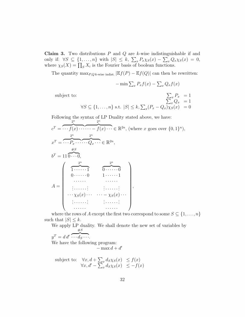
The quantity maxP,Qk-wise indist. |Ef(P )− Ef(Q)| can then be rewritten:

−min∑

x Pxf(x)−∑

xQxf(x)

subject to:∑

x Px = 1∑xQx = 1

∀S ⊆ 1, . . . , n s.t. |S| ≤ k,∑

x(Px −Qx)χS(x) = 0

Following the syntax of LP Duality stated above, we have:

cT =

2n︷ ︸︸ ︷· · · f(x) · · ·

2n︷ ︸︸ ︷· · · − f(x) · · · ∈ R2n, (where x goes over 0, 1n),

xT =

2n︷ ︸︸ ︷· · ·Px · · ·

2n︷ ︸︸ ︷· · ·Qx · · · ∈ R2n,

bT = 11

#S︷ ︸︸ ︷0 · · · 0,

A =

2n︷ ︸︸ ︷1 · · · · · · 1

2n︷ ︸︸ ︷0 · · · · · · 0

0 · · · · · · 0 1 · · · · · · 1· · · · · · · · · · · ·

... · · · · · · ... ... · · · · · · ...· · ·χS(x) · · · · · · − χS(x) · · ·

... · · · · · · ... ... · · · · · · ...· · · · · · · · · · · ·

,

where the rows ofA except the first two correspond to some S ⊆ 1, . . . , nsuch that |S| ≤ k.

We apply LP duality. We shall denote the new set of variables by

yT = d d′#S︷ ︸︸ ︷

· · · dS · · ·.We have the following program:

−max d+ d′

subject to: ∀x, d+∑

x dSχS(x) ≤ f(x)∀x, d′ −

∑x dSχS(x) ≤ −f(x)

32

Writing d′ = −d − ε, the objective becomes to minimize ε, while thesecond set of constraints can be rewritten:

∀x, d+ ε+∑S

dSχS(x) ≥ f(x) .

The expression d+∑

S dSχS(X) is an arbitrary degree-k polynomial whichwe denote by g(X). So our constrains become

g(x) ≤ f(x)

g(x) + ε ≥ f(x).

Where g ranges over all degree-k polynomials, and we are trying to min-imize ε. Because g is always below f , but when you add ε it becomes bigger,g is always within ε of f .

4.2 Approximate Degree of AND.

Let us now study the AND function on n bits. Let us denote dε(f) theminimal degree of a polynomial approximating f with error ε.

We will show that d1/3(AND) = Θ(√n).

Let us first show the upper bound:

Claim 4. We have:d1/3(AND) = O(

√n).

To prove this claim, we will consider a special family of polynomials:

Definition 5. (Chebychev polynomials of the first kind.)The Chebychev polynomials (of the first kind) are a family Tkk∈N of

polynomials defined inductively as:

• T0(X) := 1,

• T1(X) := X,

• ∀k ≥ 1, Tk+1(X) := 2XTk − Tk−1.

Those polynomials satisfy some useful properties:

1. ∀x ∈ [−1, 1], Tk(x) = cos(k arccos(x)) ,

33

2. ∀x ∈ [−1, 1],∀k, |Tk(x)| ≤ 1 ,

3. ∀x such that |x| ≥ 1, |T ′k(x)| ≥ k2 ,

4. ∀k, Tk(1) = 1 .

Property 2 follows from 1, and property 4 follows from a direct induction.For a nice picture of these polynomials you should have come to class (or Iguess you can check wikipedia). We can now prove our upper bound:

Proof. Proof of Claim:We construct a univariate polynomial p : 0, 1, . . . , n → R such that:

• deg p = O(√n);

• ∀i < n, |P (i)| ≤ 1/3;

• |P (n)− 1| ≤ 1/3.

In other words, p will be close to 0 on [0, n−1], and close to 1 on n. Then,we can naturally define the polynomial for the AND function on n bits to beq(X1, . . . , Xn) := p(

∑iXi), which also has degree O(

√n). Indeed, we want

q to be close to 0 if X has Hamming weight less than n, while being close to1 on X of Hamming weight n (by definition of AND). This will conclude theproof.

Let us define p as follows:

∀i ≤ n, p(i) :=Tk(

in−1

)Tk(

nn−1

) .Intuitively, this uses the fact that Chebychev polynomials are bounded in[−1, 1] (Property 2.) and then increase very fast (Property 3.).

More precisely, we have:

• p(n) = 1 by construction;

• for i < n, we have:

Tk(

in−1

)≤ 1 by Property 2.;

Tk(

nn−1

)= Tk

(1 + 1

n−1

)≥ 1+ k2

n−1by Property 3. and 4., and therefore

for some k = O(√n), we have: Tk

(nn−1

)≥ 3.

34

Let us now prove the corresponding lower bound:

Claim 6. We have:d1/3(AND) = Ω(

√n).

Proof. Let p be a polynomial that approximates the AND function with error1/3. Consider the univariate symmetrization p′ of p.

We have the following result from approximation theory:

Theorem 7. Let q be a real univariate polynomial such that:

1. ∀i ∈ 0, . . . , n, |q(i)| ≤ O(1);

2. q′(x) ≥ Ω(1) for some x ∈ [0, n].

Then deg q = Ω(√n).

To prove our claim, it is therefore sufficient to check that p′ satisfiesconditions 1. and 2., as we saw that deg p ≥ deg p′:

1. We have: ∀i ∈ 0, . . . , n, |p′(i)| ≤ 1 + 1/3 by assumption on p;

2. We have p′(n− 1) ≤ 1/3 and p′(n) ≥ 2/3 (by assumption), so that themean value theorem gives some x such that p′(x) ≥ Ω(1).

This concludes the proof.

4.3 Approximate Degree of AND-OR.

Consider the AND function on R bits and the OR function on N bits. LetAND-OR: 0, 1R×N → 0, 1 be their composition (which outputs the ANDof the R outputs of the OR function on N -bits (disjoint) blocks).

It is known that d1/3(AND-OR) = Θ(√RN). To prove the upper bound,

we will need a technique to compose approximating polynomials which wewill discuss later.

Now we focus on the lower bound. This lower bound was recently provedindependently by Sherstov and by Bun and Thaler. We present a proofthat is different (either in substance or in language) and which we find more

35

intuitive. Our proof replaces the “dual block method” with the followinglemma.

Lemma 8. Suppose thatdistributions A0, A1 over 0, 1nA are kA-wise indistinguishable distribu-

tions; anddistributions B0, B1 over 0, 1nB are kB-wise indistinguishable distribu-

tions.Define C0, C1 over 0, 1nA·nB as follows: Cb: draw a sample x ∈ 0, 1nA

from Ab, and replace each bit xi by a sample of Bxi (independently).Then C0 and C1 are kA · kB-wise indistinguishable.

Proof. Consider any set S ⊆ 1, . . . , nA · nB of kA · kB bit positions; let usshow that they have the same distribution in C0 and C1.

View the nA ·nB as nA blocks of nB bits. Call a block K of nB bits heavyif |S ∩K| ≥ kB; call the other blocks light.

There are at most kA heavy blocks by assumption, so that the distri-bution of the (entire) heavy blocks are the same in C0 and C1 by kA-wiseindistinguishability of A0 and A1.

Furthermore, conditioned on any outcome for the Ab samples in Cb, thelight blocks have the same distribution in both C0 and C1 by kB-wise indis-tinguishability of B0 and B1.

Therefore C0 and C1 are kA · kB-wise indistinguishable.

4.4 Lower Bound of d1/3(AND-OR)

To prove the lower bound on the approximate degree of the AND-OR func-tion, it remains to see that AND-OR can distinguish well the distributionsC0 and C1. For this, we begin with observing that we can assume withoutloss of generality that the distributions have disjoint supports.

Claim 9. For any function f , and for any k-wise indistinguishable distribu-tions A0 and A1, if f can distinguish A0 and A1 with probability ε then thereare distributions B0 and B1 with the same properties (k-wise indistinguisha-bility yet distinguishable by f) and also with disjoint supports. (By disjointsupport we mean for any x either Pr[B0 = x] = 0 or Pr[B1 = x] = 0.)

Proof. Let distribution C be the “common part” of A0 and A1. That isto say, we define C such that Pr[C = x] := minPr[A0 = x],Pr[A1 = x]

36

multiplied by some constant that normalize C into a distribution.Then we can write A0 and A1 as

A0 = pC + (1− p)B0 ,

A1 = pC + (1− p)B1 ,

where p ∈ [0, 1], B0 and B1 are two distributions. Clearly B0 and B1 havedisjoint supports.

Then we have

E[f(A0)]− E[f(A1)] = pE[f(C)] + (1− p)E[f(B0)]

− pE[f(C)]− (1− p)E[f(B1)]

= (1− p)(E[f(B0)]− E[f(B1)]

)≤ E[f(B0)]− E[f(B1)] .

Therefore if f can distinguish A0 and A1 with probability ε then it can alsodistinguish B0 and B1 with such probability.

Similarly, for all S 6= ∅ such that |S| ≤ k, we have

0 = E[χS(A0)]− E[χS(A1)] = (1− p)(E[χS(B0)]− E[χS(B1)]

)= 0 .

Hence, B0 and B1 are k-wise indistinguishable.

Equipped with the above lemma and claim, we can finally prove thefollowing lower bound on the approximate degree of AND-OR.

Theorem 10. d1/3(AND-OR) = Ω(√RN).

Proof. Let A0, A1 be Ω(√R)-wise indistinguishable distributions for AND

with advantage 0.99, i.e. Pr[AND(A1) = 1] > Pr[AND(A0) = 1] + 0.99. LetB0, B1 be Ω(

√N)-wise indistinguishable distributions for OR with advantage

0.99. By the above claim, we can assume that A0, A1 have disjoint supports,and the same for B0, B1. Compose them by the lemma, getting Ω(

√RN)-

wise indistinguishable distributions C0, C1. We now show that AND-OR candistinguish C0, C1:

• C0: First sample A0. As there exists a unique x = 1R such thatAND(x) = 1, Pr[A1 = 1R] > 0. Thus by disjointness of supportPr[A0 = 1R] = 0. Therefore when sampling A0 we always get a stringwith at least one “0”. But then “0” is replaced with sample from B0.We have Pr[B0 = 0N ] ≥ 0.99, and when B0 = 0N , AND-OR= 0.

37

• C1: First sample A1, and we know that A1 = 1R with probability atleast 0.99. Each bit “1” is replaced by a sample from B1, and we knowthat Pr[B1 = 0N ] = 0 by disjointness of support. Then AND-OR= 1.

Therefore we have d1/3(AND-OR) = Ω(√RN).

4.5 Lower Bound of d1/3(SURJ)

In this subsection we discuss the approximate degree of the surjectivity func-tion. This function is defined as follows.

Definition 11. The surjectivity function SURJ:(0, 1logR

)N → 0, 1,which takes input (x1, . . . , xN) where xi ∈ [R] for all i, has value 1 if andonly if ∀j ∈ [R],∃i : xi = j.

First, some history. Aaronson first proved that the approximate degreeof SURJ and other functions on n bits including “the collision problem” isnΩ(1). This was motivated by an application in quantum computing. Beforethis result, even a lower bound of ω(1) had not been known. Later Shiimproved the lower bound to n2/3, see [AS04]. The instructor believes thatthe quantum framework may have blocked some people from studying thisproblem, though it may have very well attracted others. Recently Bun andThaler [BT17] reproved the n2/3 lower bound, but in a quantum-free paper,and introducing some different intuition. Soon after, together with Kothari,they proved [BKT17] that the approximate degree of SURJ is Θ(n3/4).

We shall now prove the Ω(n3/4) lower bound, though one piece is onlysketched. Again we present some things in a different way from the papers.

For the proof, we consider the AND-OR function under the promise thatthe Hamming weight of the RN input bits is at mostN . Call the approximatedegree of AND-OR under this promise d≤N1/3 (AND-OR). Then we can provethe following theorems.

Theorem 12. d1/3(SURJ) ≥ d≤N1/3 (AND-OR).

Theorem 13. d≤N1/3 (AND-OR) ≥ Ω(N3/4) for some suitable R = Θ(N).

In our settings, we consider R = Θ(N). Theorem 12 shows surprisinglythat we can somehow “shrink” Θ(N2) bits of input into N logN bits whilemaintaining the approximate degree of the function, under some promise.Without this promise, we just showed in the last subsection that the ap-

38

proximate degree of AND-OR is Ω(N) instead of Ω(N3/4) as in Theorem13.

Proof of Theorem 12. Define an N × R matrix Y s.t. the 0/1 variable yij isthe entry in the i-th row j-th column, and yij = 1 iff xi = j. We can provethis theorem in following steps:

1. d1/3(SURJ(x)) ≥ d1/3(AND-OR(y)) under the promise that each rowhas weight 1;

2. let zj be the sum of the j-th column, then d1/3(AND-OR(y)) under thepromise that each row has weight 1, is at least d1/3(AND-OR(z)) underthe promise that

∑j zj = N ;

3. d1/3(AND-OR(z)) under the promise that∑

j zj = N , is at least d=N1/3 (AND-

OR(y));

4. we can change “= N” into “≤ N”.

Now we prove this theorem step by step.

1. Let P (x1, . . . , xN) be a polynomial for SURJ, where xi = (xi)1, . . . , (xi)logR.Then we have

(xi)k =∑

j:k-th bit of j is 1

yij.

Then the polynomial P ′(y) for AND-OR(y) is the polynomial P (x) with(xi)k replaced as above, thus the degree won’t increase. Correctnessfollows by the promise.

2. This is the most extraordinary step, due to Ambainis [Amb05]. In thisnotation, AND-OR becomes the indicator function of ∀j, zj 6= 0. Define

Q(z1, . . . , zR) := Ey: his rows have weight 1and is consistent with z

P (y).

Clearly it is a good approximation of AND-OR(z). It remains to showthat it’s a polynomial of degree k in z’s if P is a polynomial of degreek in y’s.

39

Let’s look at one monomial of degree k in P : yi1j1yi2j2 · · · yikjk . Observethat all i`’s are distinct by the promise, and by u2 = u over 0, 1. Bychain rule we have

E[yi1j1 · · · yikjk ] = E[yi1j1 ]E[yi2j2|yi1j1 = 1] · · ·E[yikjk |yi1j1 = · · · = yik−1jk−1= 1].

By symmetry we have E[yi1j1 ] =zj1

N, which is linear in z’s. To get

E[yi2j2|yi1j1 = 1], we know that every other entry in row i1 is 0, so we

give away row i1, average over y’s such that

yi1j1 = 1yij = 0 j 6= j1

under

the promise and consistent with z’s. Therefore

E[yi2j2|yi1j1 = 1] =

zj2

N−1j1 6= j2,

zj2−1

N−1j1 = j2.

In general we have

E[yikjk |yi1j1 = · · · = yik−1jk−1= 1] =

zjk −#` < k : j` = jkN − k + 1

,

which has degree 1 in z’s. Therefore the degree of Q is not larger thanthat of P .

3. Note that ∀j, zj =∑

i yij. Hence by replacing z’s by y’s, the degreewon’t increase.

4. We can add a “slack” variable z0, or equivalently y01, . . . , y0N ; then thecondition

∑Rj=0 zj = N actually means

∑Rj=1 zj ≤ N .

Proof idea for Theorem 13. First, by the duality argument we can verify thatd≤N1/3 (f) ≥ d if and only if there exists d-wise indistinguishable distributionsA,B such that:

• f can distinguish A,B;

• A and B are supported on strings of weight ≤ N .

40

Claim 14. d≤√N

1/3 (ORN) = Ω(N1/4).

The proof needs a little more information about the weight distributionof the indistinguishable distributions corresponding to this claim. Basically,their expected weight is very small.

Now we combine these distributions with the usual ones for And usingthe lemma mentioned at the beginning.

What remains to show is that the final distribution is supported on Ham-ming weight ≤ N . Because by construction the R copies of the distributionsfor Or are sampled independently, we can use concentration of measure toprove a tail bound. This gives that all but an exponentially small measure ofthe distribution is supported on strings of weight ≤ N . The final step of theproof consists of slightly tweaking the distributions to make that measure0.

5 Pseudorandom groups and communication

complexity

Groups have many applications in theoretical computer science. Barrington[Bar89] used the permutation group S5 to prove a very surprising result,which states that the majority function can be computed efficiently usingonly constant bits of memory (something which was conjectured to be false).More recently, catalytic computation [BCK+14] shows that if we have a lotof memory, but it’s full with junk that cannot be erased, we can still computemore than if we had little memory. We will see some interesting propertiesof groups in the following.

Some famous groups used in computer science are:

• 0, 1n with bit-wise addition;

• Zm with addition mod m ;

• Sn, which are permutations of n elements;

• Wreath product G := (Zm × Zm) o Z2 , whose elements are of the form(a, b)z where z is a “flip bit”, with the following multiplication rules:

– (a, b)1 = 1(b, a) ;

– z · z′ := z + z′ in Z2 ;

41

– (a, b) · (a′, b′) := (a+ a′, b+ b′) is the Zm × Zm operation;

An example is (5, 7)1 · (2, 1)1 = (5, 7)1 · 1(1, 2) = (6, 9)0 . Generally wehave

(a, b)z · (a′, b′)z′ =

(a+ a′, b+ b′)z + z′ z = 1 ,(a+ b′, b+ a′)z + z′ z = 0 ;

• SL2(q) := 2×2 matrices over Fq with determinant 1, in other words,

group of matrices

(a bc d

)such that ad− bc = 1.

The group SL2(q) was invented by Galois. (If you haven’t, read hisbiography on wikipedia.)

Quiz. Among these groups, which is the “least abelian”? The latter canbe defined in several ways. We focus on this: If we have two high-entropydistributions X, Y over G, does X · Y has more entropy? For example, ifX and Y are uniform over some Ω(|G|) elements, is X · Y close to uniformover G? By “close to” we mean that the statistical distance is less that asmall constant from the uniform distribution. For G = (0, 1n,+), if Y = Xuniform over 0× 0, 1n−1, then X · Y is the same, so there is not entropyincrease even though X and Y are uniform on half the elements.

Definition 1.[Measure of Entropy] For ‖A‖2 = (∑

xA(x)2)12 , we think of

‖A‖22 = 100 1

|G| for “high entropy”.

Note that ‖A‖22 is exactly the “collision probability”, i.e. Pr[A = A′].

We will consider the entropy of the uniform distribution U as very small, i.e.‖U‖2

2 = 1|G| ≈ ‖0‖

22. Then we have

‖A− U‖22 =

∑x

(A(x)− 1

|G|

)2

=∑x

A(x)2 − 2A(x)1

|G|+

1

|G|2

= ‖A‖22 −

1

|G|= ‖A‖2

2 − ‖U‖22

≈ ‖A‖22 .

42

Theorem 2.[[Gow08], [BNP08]] If X, Y are independent over G, then

‖X · Y − U‖2 ≤ ‖X‖2‖Y ‖2

√|G|d,

where d is the minimum dimension of irreducible representation of G.

By this theorem, for high entropy distributions X and Y , we get ‖X ·Y −U‖2 ≤ O(1)√

|G|d, thus we have

‖X · Y − U‖1 ≤√|G|‖X · Y − U‖2 ≤

O(1)√d. (1)

If d is large, then X · Y is very close to uniform. The following table showsthe d’s for the groups we’ve introduced.

G 0, 1n Zm (Zm × Zm) o Z2 An SL2(q)

d 1 1 should be very small log |G|log log |G| |G|1/3

Here An is the alternating group of even permutations. We can see thatfor the first groups, Equation (1) doesn’t give non-trivial bounds.

But for An we get a non-trivial bound, and for SL2(q) we get a strongbound: we have ‖X · Y − U‖2 ≤ 1

|G|Ω(1) .

We now study the communication complexity of some problems on groups.We give the definition of a protocol when two parties are involved and gen-eralize later to more parties.

Definition 3. A 2-party c-bit deterministic communication protocol is adepth-c binary tree such that:

• the leaves are the output of the protocol

• each internal node is labeled with a party and a function from thatparty’s input space to 0, 1

Computation is done by following a path on edges, corresponding to out-puts of functions at the nodes.

A public-coin randomized protocol is a distribution on deterministic pro-tocols.

43

5.1 2-party communication protocols

We start with a simple protocol for the following problem.Let G be a group. Alice gets x ∈ G and Bob gets y ∈ G and their goal is

to check if x · y = 1G, or equivalently if x = y−1.There is a simple deterministic protocol in which Alice simply sends her

input to Bob who checks if x·y = 1G. This requires O(log |G|) communicationcomplexity.

We give a randomized protocol that does better in terms on communica-tion complexity. Alice picks a random hash function h : G → 0, 1`. Wecan think that both Alice and Bob share some common randomness and thusthey can agree on a common hash function to use in the protocol. Next, Alicesends h(x) to Bob, who then checks if h(x) = h(y−1).

For ` = O(1) we get constant error and constant communication.

5.2 3-party communication protocols

There are two ways to extend 2-party communication protocols to more par-ties. We first focus on the Number-in-hand (NIH), where Alice gets x, Bobgets y, Charlie gets z, and they want to check if x · y · z = 1G. In the NIHsetting the communication depends on the group G.

5.3 A randomized protocol for the hypercube

LetG = (0, 1n,+) with addition modulo 2. We want to test if x+y+z = 0n.First, we pick a linear hash function h, i.e. satisfying h(x+ y) = h(x) +h(y).For a uniformly random a ∈ 0, 1n set ha(x) =

∑aixi (mod 2). Then,

• Alice sends ha(x)

• Bob send ha(y)

• Charlie accepts if and only if ha(x) + ha(y)︸ ︷︷ ︸ha(x+y)

= ha(z)

The hash function outputs 1 bit. The error probability is 1/2 and thecommunication is O(1). For a better error, we can repeat.

44

5.4 A randomized protocol for Zm

Let G = (Zm,+) where m = 2n. Again, we want to test if x + y + z = 0(mod m). For this group, there is no 100% linear hash function but there arealmost linear hash function families h : Zm → Z` that satisfy the followingproperties:

1. ∀a, x, y we have ha(x) + ha(y) = ha(x+ y)± 1

2. ∀x 6= 0 we have Pra[ha(x) ∈ ±2,±1, 0] ≤ 2−Ω(`)

3. ha(0) = 0

Assuming some random hash function h (from a family) that satisfies theabove properties the protocol works similar to the previous one.

• Alice sends ha(x)

• Bob sends ha(y)

• Charlie accepts if and only if ha(x) + ha(y) + ha(z) ∈ ±2,±1, 0We can set ` = O(1) to achieve constant communication and constant

error.AnalysisTo prove correctness of the protocol, first note that ha(x)+ha(y)+ha(z) =

ha(x+ y + z)± 2, then consider the following two cases:

• if x+ y + z = 0 then ha(x+ y + z)± 2 = ha(0)± 2 = 0± 2

• if x+ y + z 6= 0 then Pra[ha(x+ y + z) ∈ ±2,±1, 0] ≤ 2−Ω(`)

It now remains to show that such hash function families exist.Let a be a random odd number modulo 2n. Define

ha(x) := (a · x n− `) (mod 2`)

where the product a · x is integer multiplication. In other words we outputthe bits n− `+ 1, n− `+ 2, . . . , n of the integer product a · x.

We now verify that the above hash function family satisfies the threeproperties we required above.

Property (3) is trivially satisfied.For property (1) we have the following. Let s = a · x and t = a · y

and u = n − `. The bottom line is how (s u) + (t u) compares with(s+ t) u. In more detail we have that,

45

• ha(x+ y) = ((s+ t) u) (mod 2`)

• ha(x) = (s u) (mod 2`)

• ha(x) = (t u) (mod 2`)

Notice, that if in the addition s+ t the carry into the u+ 1 bit is 0, then

(s u) + (t u) = (s+ t) u

otherwise(s u) + (t u) + 1 = (s+ t) u

which concludes the proof for property (1).Finally, we prove property (2). We start by writing x = s · 2c where s is

odd. Bitwise, this looks like (· · · · · · 1 0 · · · 0︸ ︷︷ ︸c bits

).

The product a·x for a uniformly random a, bitwise looks like (uniform 1 0 · · · 0︸ ︷︷ ︸c bits

).

We consider the two following cases for the product a · x:

1. If a ·x = (uniform 1

2 bits︷︸︸︷00︸ ︷︷ ︸

` bits

· · · 0), or equivalently c ≥ n−`+2, the output

never lands in the bad set ±2,±1, 0 (some thought should be given tothe representation of negative numbers – we ignore that for simplicity).

2. Otherwise, the hash function output has `−O(1) uniform bits. Againfor simplicity, let B = 0, 1, 2. Thus,

Pr[output ∈ B] ≤ |B| · 2−`+O(1)

In other words, the probability of landing in any small set is small.

5.5 Other groups

What happens in other groups? Do we have an almost linear hash functionfor 2× 2 matrices? The answer is negative. For SL2(q) and An the problemof testing equality with 1G is hard.

We would like to rule out randomized protocols, but it is hard to reasonabout them directly. Instead, we are going to rule out deterministic protocolson random inputs. For concreteness our main focus will be SL2(q).

46

First, for any group element g ∈ G we define the distribution on triples,Dg := (x, y, (x · y)−1g), where x, y ∈ G are uniformly random elements. Notethe product of the elements in Dg is always g.

Towards a contradiction, suppose we have a randomized protocol P forthe xyz =? 1G problem. In particular, we have

Pr[P (D1) = 1] ≥ Pr[P (Dh) = 1] +1

10.

This implies a deterministic protocol with the same gap, by fixing the ran-domness.

We reach a contradiction by showing that for every deterministic proto-cols P using little communication (will quantify later), we have

|Pr[P (D1) = 1]− Pr[P (Dh) = 1]| ≤ 1

100.

We start with the following lemma, which describes a protocol usingproduct sets.

Lemma 4. (The set of accepted inputs of) A deterministic c-bit protocolcan be written as a disjoint union of 2c “rectangles,” that is sets of the formA×B × C.

Proof. (sketch) For every communication transcript t, let St ⊆ G3 be the setof inputs giving transcript t. The sets St are disjoint since an input givesonly one transcript, and their number is 2c, i.e. one for each communicationtranscript of the protocol. The rectangle property can be proven by inductionon the protocol tree.

Next, we show that these product sets cannot distinguish these two dis-tributions D1, Dh, and for that we will use the pseudorandom properties ofthe group G.

Lemma 5. For all A,B,C ⊆ G and we have

|Pr[A×B × C(D1) = 1]− Pr[A×B × C(Dh) = 1]| ≤ 1

dΩ(1).

Recall the parameter d from the previous lectures and that when thegroup G is SL2(q) then d = |G|Ω(1).

47

Proof. Pick any h ∈ G and let x, y, z be the inputs of Alice, Bob, and Charlierespectively. Then

Pr[A×B×C(Dh) = 1] = Pr[(x, y) ∈ A×B]·Pr[(x·y)−1 ·h ∈ C|(x, y) ∈ A×B]

If either A or B is small, that is Pr[x ∈ A] ≤ ε or Pr[y ∈ B] ≤ ε, thenalso Pr[P (Dh) = 1] ≤ ε because the term Pr[(x, y) ∈ A × B] will be small.We will choose ε later.

Otherwise, A and B are large, which implies that x and y are uniform overat least ε|G| elements. Recall from Lecture 9 that this implies ‖x · y−U‖2 ≤‖x‖2 · ‖y‖2 ·

√|G|d

, where U is the uniform distribution.

By Cauchy–Schwarz we obtain,

‖x · y − U‖1 ≤ |G| · ‖x‖2 · ‖y‖2 ·√

1

d≤ 1

ε· 1√

d.

The last inequality follows from the fact that ‖x‖2, ‖y‖2 ≤√

1ε|G| .

This implies that ‖(x · y)−1 − U‖1 ≤ 1ε· 1√

dand ‖(x · y)−1 · h − U‖1 ≤

1ε· 1√

d, because taking inverses and multiplying by h does not change anything.

These two last inequalities imply that,

Pr[(x · y)−1 ∈ C|(x, y) ∈ A×B] = Pr[(x · y)−1 ·h ∈ C|(x, y) ∈ A×B]± 2

ε

1√d

and thus we get that,

Pr[P (D1) = 1] = Pr[P (Dh) = 1]± 2

ε

1√d.

To conclude, based on all the above we have that for all ε and independentof the choice of h, it is either the case that

|Pr[P (D1) = 1]− Pr[P (Dh) = 1]| ≤ 2ε

or

|Pr[P (D1) = 1]− Pr[P (Dh) = 1]| ≤ 2

ε

1√d

and we will now choose the ε to balance these two cases and finish the proof:

2

ε

1√d

= 2ε⇔ 1√d

= ε2 ⇔ ε =1

d1/4.

48

The above proves that the distribution Dh behaves like the uniform dis-tribution for product sets, for all h ∈ G.

Returning to arbitrary deterministic protocols P , write P as a union of2c disjoint rectangles by the first lemma. Applying the second lemma andsumming over all rectangles we get that the distinguishing advantage of Pis at most 2c/d1/4. For c ≤ (1/100) log d the advantage is at most 1/100 andthus we get a contradiction on the existence of such a correct protocol. Wehave concluded the proof of this theorem.

Theorem 6. Let G be a group, and d be the minimum dimension of anirreducible representation of G. Consider the 3-party, number-in-hand com-munication protocol f : G3 → 0, 1 where f(x, y, z) = 1 ⇔ x · y · z = 1G.Its randomized communication complexity is Ω(log d).

For SL2(q) the communication is Ω(log |G|). This is tight up to constants,because Alice can send her entire group element.

For the groupAn the known bounds on d yield communication Ω(log log |G|).This bound is tight for the problem of distinguishing D1 from Dh for h 6= 1,as we show next. The identity element 1G for the group An is the identity per-mutation. If h 6= 1G then h is a permutation that maps some element a ∈ Gto h(a) = b 6= a. The idea is that the parties just need to “follow” a, which islogarithmically smaller than G. Specifically, let x, y, z be the permutationsthat Alice, Bob and Charlie get. Alice sends x(a) ∈ [n]. Bob gets x(a) andsends y(x(a)) ∈ [n] to Charlie who checks if z(y(x(a))) = 1. The communi-cation is O(log n). Because the size of the group is |G| = Θ(n!) = Θ

((ne

)n),

the communication is O(log log |G|).This is also a proof that d cannot be too large for An, i.e. is at most

(log |G|)O(1).

5.6 More on 2-party protocols

We move to another setting where a clean answer can be given. Here we onlyhave two parties. Alice gets x1, x2, . . . , xn, Bob gets y1, y2, . . . , yn, and theywant to know if x1 · y1 · x2 · y2 · · ·xn · yn = 1G.

When G is abelian, the elements can be reordered as to check whether(x1 · x2 · · · xn) · (y1 · y2 · · · yn) = 1G. This requires constant communication(using randomness) as we saw in Lecture 12, since it is equivalent to thecheck x · y = 1G where x = x1 · x2 · · · xn and y = y1 · y2 · · · yn.

We will prove the next theorem for non-abelian groups.

49

Theorem 7. For every non-abelian group G the communication of decidingif x1 · y1 · x2 · y2 · · ·xn · yn = 1G is Ω(n).

Proof. We reduce from unique disjointness, defined below. For the reductionwe will need to encode the And of two bits x, y ∈ 0, 1 as a group product.(This question is similar to a puzzle that asks how to hang a picture on thewall with two nails, such that if either one of the nails is removed, the picturewill fall. This is like computing the And function on two bits, where both bits(nails) have to be 1 in order for the function to be 1.) Since G is non-abelian,there exist a, b ∈ G such that a · b 6= b · a, and in particular a · b · a−1 · b−1 = hwith h 6= 1. We can use this fact to encode And as

ax · by · a−x · b−y =

1, if And(x,y)=0

h, otherwise.

In the disjointness problem Alice and Bob get inputs x, y ∈ 0, 1n respec-tively, and they wish to check if there exists an i ∈ [n] such that xi ∧ yi = 1.If you think of them as characteristic vectors of sets, this problem is asking ifthe sets have a common element or not. The communication of this problemis Ω(n). Moreover, in the variant of this problem where the number of suchi’s is 0 or 1 (i.e. unique), the same lower bound Ω(n) still applies. This is likegiving Alice and Bob two sets that either are disjoint or intersect in exactlyone element, and they need to distinguish these two cases.

Next, we will reduce the above variant of the set disjointness to groupproducts. For x, y ∈ 0, 1n we product inputs for the group problem asfollows:

x→ (ax1 , a−x1 , . . . , axn , a−xn)

y → (by1 , b−y1 , . . . , byn , b−yn).

Now, the product x1 ·y1 ·x2 ·y2 · · · xn ·yn we originally wanted to computebecomes

ax1 · by1 · a−x1 · b−y1︸ ︷︷ ︸1 bit

· · · · · · axn · byn · a−xn · b−yn .

If there isn’t an i ∈ [n] such that xi ∧ yi = 1, then each product termaxi · byi · a−xi · b−yi is 1 for all i, and thus the whole product is 1.

Otherwise, there exists a unique i such that xi ∧ yi = 1 and thus theproduct will be 1 · · · 1 · h · 1 · · · 1 = h, with h being in the i-th position. If

50

Alice and Bob can test if the above product is equal to 1, they can also solvethe unique set disjointness problem, and thus the lower bound applies for theformer.

We required the uniqueness property, because otherwise we might get aproduct hc that could be equal to 1 in some groups.

6 Number-on-forehead communication com-

plexity

In number-on-forehead (NOH) communication complexity each party i seesall of the input (x1, . . . , xk) except its own input xi. For background, it isnot known how to prove negative results for k ≥ log n parties. We shall focuson the problem of separating deterministic and randomizes communication.For k = 2, we know the optimal separation: The equality function requiresΩ(n) communication for deterministic protocols, but can be solved usingO(1) communication if we allow the protocols to use public coins. For k = 3,the best known separation between deterministic and randomized protocolis Ω(log n) vs O(1) [BDPW10]. In the following we give a new proof of thisresult, for a simpler function: f(x, y, z) = 1 if and only if x · y · z = 1 forx, y, z ∈ SL2(q).

For context, let us state and prove the upper bound for randomized com-munication.

Claim 1. f has randomized communication complexity O(1).

Proof. In the NOH model, computing f reduces to 2-party equality with noadditional communication: Alice computes y · z =: w privately, then Aliceand Bob check if x = w−1.

To prove a Ω(log n) lower bound for deterministic protocols, where n =log |G|, we reduce the communication problem to a combinatorial problem.

Definition 2. A corner in a group G is (x, y), (xz, y), (x, zy) ⊆ G2, wherex, y are arbitrary group elements and z 6= 1G.

For intuition, consider the case when G is Abelian, where one can replacemultiplication by addition and a corner becomes (x, y), (x+z, y), (x, y+z)for z 6= 0.

51

We now state the theorem that gives the lower bound.

Theorem 3. Suppose that every subset A ⊆ G2 with µ(A) := |A|/|G2| ≥δ contains a corner. Then the deterministic communication complexity off(x, y, z) = 1 ⇐⇒ x · y · z = 1G is Ω(log(1/δ)).

It is known that when G is Abelian, then δ ≥ 1/polyloglog|G| implies acorner. We shall prove that when G = SL2(q), then δ ≥ 1/polylog|G| impliesa corner. This in turn implies communication Ω(log log |G|) = Ω(log n).

Proof. We saw that a number-in-hand (NIH) c-bit protocol can be writtenas a disjoint union of 2c rectangles. Likewise, a number-on-forehead c-bitprotocol P can be written as a disjoint union of 2c cylinder intersectionsCi := (x, y, z) : fi(y, z)gi(x, z)hi(x, y) = 1 for some fi, gi, hi : G

2 → 0, 1:

P (x, y, z) =2c∑i=1

fi(y, z)gi(x, z)hi(x, y).

The proof idea of the above fact is to consider the 2c transcripts of P , then onecan see that the inputs giving a fixed transcript are a cylinder intersection.

Let P be a c-bit protocol. Consider the inputs (x, y, (xy)−1) on whichP accepts. Note that at least 2−c fraction of them are accepted by somecylinder intersection C. Let A := (x, y) : (x, y, (xy)−1) ∈ C ⊆ G2. Sincethe first two elements in the tuple determine the last, we have µ(A) ≥ 2−c.

Now suppose A contains a corner (x, y), (xz, y), (x, zy). Then

(x, y) ∈ A =⇒ (x, y, (xy)−1) ∈ C =⇒ h(x, y) = 1,

(xz, y) ∈ A =⇒ (xz, y, (xzy)−1) ∈ C =⇒ f(y, (xyz)−1) = 1,

(x, zy) ∈ A =⇒ (x, zy, (xzy)−1) ∈ C =⇒ g(x, (xyz)−1) = 1.

This implies (x, y, (xzy)−1) ∈ C, which is a contradiction because z 6= 1 andso x · y · (xzy)−1 6= 1G.

7 Corners in pseudorandom groups

In this section we prove the corners theorem for pseudorandom groups, fol-lowing Austin [Aus16]. Our exposition has several non-major differences withthat in [Aus16], which may make it more computer-science friendly. The in-structor suspects a proof can also be obtained via certain local modifications

52

and simplifications of Green’s exposition [Gre05b, Gre05a] of an earlier prooffor the abelian case. We focus on the case G = SL2(q) for simplicity, but theproof immediately extends to other pseudorandom groups.

Theorem 1. Let G = SL2(q). Every subset A ⊆ G2 of density µ(A) ≥1/ loga |G| contains a corner, i.e., a set of the form (x, y), (xz, y), (x, zy) | z 6=1.

7.1 Proof Overview

For intuition, suppose A is a product set, i.e., A = B × C for B,C ⊆ G.Let’s look at the quantity

Ex,y,z←G[A(x, y)A(xz, y)A(x, zy)]

where A(x, y) = 1 iff (x, y) ∈ A. Note that the random variable in theexpectation is equal to 1 exactly when x, y, z form a corner in A. We’ll showthat this quantity is greater than 1/|G|, which implies that A contains acorner (where z 6= 1). Since we are taking A = B × C, we can rewrite theabove quantity as

Ex,y,z←G[B(x)C(y)B(xz)C(y)B(x)C(zy)]

= Ex,y,z←G[B(x)C(y)B(xz)C(zy)]

= Ex,y,z←G[B(x)C(y)B(z)C(x−1zy)]

where the last line follows by replacing z with x−1z in the uniform distri-bution. If µ(A) ≥ δ, then µ(B) ≥ δ and µ(C) ≥ δ. Condition on x ∈ B,y ∈ C, z ∈ B. Then the distribution x−1zy is a product of three independentdistributions, each uniform on a set of measure greater than δ. By pseudo-randomness x−1zy is 1/|G|Ω(1) close to uniform in statistical distance. Thisimplies that the above quantity equals

µ(A) · µ(C) · µ(B) ·(µ(C)± 1

|G|Ω(1)

)≥ δ3

(δ − 1

|G|Ω(1)

)≥ δ4/2

> 1/|G|.Given this, it is natural to try to write an arbitrary A as a combination

of product sets (with some error). We will make use of a more general result.

53

7.2 Weak Regularity Lemma

Let U be some universe (we will take U = G2). Let f : U → [−1, 1] bea function (for us, f = 1A). Let D ⊆ d : U → [−1, 1] be some set offunctions, which can be thought of as “easy functions” or “distinguishers.”

Theorem 2.[Weak Regularity Lemma] For all ε > 0, there exists a functiong :=

∑i≤s ci · di where di ∈ D, ci ∈ R and s = 1/ε2 such that for all d ∈ D

Ex←U [f(x) · d(x)] = Ex←U [g(x) · d(x)]± ε.

The lemma is called ‘weak’ because it came after Szemeredi’s regularitylemma, which has a stronger distinguishing conclusion. However, the lemmais also ‘strong’ in the sense that Szemeredi’s regularity lemma has s as atower of 1/ε whereas here we have s polynomial in 1/ε. The weak regularitylemma is also simpler. There also exists a proof of Szemeredi’s theorem (onarithmetic progressions), which uses weak regularity as opposed to the fullregularity lemma used initially.

Proof. We will construct the approximation g through an iterative processproducing functions g0, g1, . . . , g. We will show that ||f − gi||22 decreases by≥ ε2 each iteration.

1. Start: Define g0 = 0 (which can be realized setting c0 = 0).

2. Iterate: If not done, there exists d ∈ D such that |E[(f − g) · d]| > ε.Assume without loss of generality E[(f − g) · d] > ε.

3. Update: g′ := g + λd where λ ∈ R shall be picked later.

Let us analyze the progress made by the algorithm.

||f − g′||22 = Ex[(f − g′)2(x)]

= Ex[(f − g − λd)2(x)]

= Ex[(f − g)2] + Ex[λ2d2(x)]− 2Ex[(f − g) · λd(x)]

≤ ||f − g||22 + λ2 − 2λEx[(f − g)d(x)]

≤ ||f − g||22 + λ2 − 2λε

≤ ||f − g||22 − ε2

where the last line follows by taking λ = ε. Therefore, there can only be 1/ε2

iterations because ||f − g0||22 = ||f ||22 ≤ 1.

54

7.3 Getting more for rectangles

Returning to the lower bound proof, we will use the weak regularity lemma toapproximate the indicator function for arbitrary A by rectangles. That is, wetake D to be the collection of indicator functions for all sets of the form S×Tfor S, T ⊆ G. The weak regularity lemma gives us A as a linear combinationof rectangles. These rectangles may overlap. However, we ideally want A tobe a linear combination of non-overlapping rectangles.

Claim 3. Given a decomposition of A into rectangles from the weak regular-ity lemma with s functions, there exists a decomposition with 2O(s) rectangleswhich don’t overlap.

Proof. Exercise.

In the above decomposition, note that it is natural to take the coefficientsof rectangles to be the density of points in A that are in the rectangle. Thisgives rise to the following claim.

Claim 4. The weights of the rectangles in the above claim can be the averageof f in the rectangle, at the cost of doubling the distinguisher error.

Consequently, we have that f = g + h, where g is the sum of 2O(s) non-overlapping rectangles S × T with coefficients Pr(x,y)∈S×T [f(x, y) = 1].

Proof. Let g be a partition decomposition with arbitrary weights. Let g′ bea partition decomposition with weights being the average of f . It is enoughto show that for all rectangle distinguishers d ∈ D

|E[(f − g′)d]| ≤ |E[(f − g)d]|.

By the triangle inequality, we have that

|E[(f − g′)d]| ≤ |E[(f − g)d]|+ |E[(g − g′)d]|.

To bound E[(g − g′)d]|, note that the error is maximized for a d that re-spects the decomposition in non-overlapping rectangles, i.e., d is the unionof some non-overlapping rectangles from the decomposition. This can beargues using that, unlike f , the value of g and g′ on a rectangle S × Tfrom the decomposition is fixed. But, for such d, g′ = f ! More formally,E[(g − g′)d] = E[(g − f)d].

55

We need to get a little more from this decomposition. The conclusion ofthe regularity lemma holds with respect to distinguishers that can be writtenas U(x) ·V (y) where U and V map G→ 0, 1. We need the same guaranteefor U and V with range [−1, 1]. This can be accomplished paying only aconstant factor in the error, as follows. Let U and V have range [−1, 1].Write U = U+ − U− where U+ and U− have range [0, 1], and the same forV . The error for distinguisher U · V is at most the sum of the errors fordistinguishers U+ · V+, U+ · V−, U− · V+, and U− · V−. So we can restrictour attention to distinguishers U(x) · V (y) where U and V have range [0, 1].In turn, a function U(x) with range [0, 1] can be written as an expectationEaUa(x) for functions Ua with range 0, 1, and the same for V . We concludeby observing that

Ex,y[(f − g)(x, y)EaUa(x) · EbVb(y)] ≤ maxa,b

Ex,y[(f − g)(x, y)Ua(x) · Vb(y)].

7.4 Proof

Let us now finish the proof by showing a corner exists for sufficiently densesets A ⊆ G2. We’ll use three types of decompositions for f : G2 → 0, 1,with respect to the following three types of distinguishers, where Ui and Vihave range 0, 1:

1. U1(x) · V1(y),

2. U2(xy) · V2(y),

3. U3(x) · V3(xy).

The last two distinguishers can be visualized as parallelograms with a 45-degree angle between two segments. The same extra properties we discussedfor rectangles hold for them too.

Recall that we want to show

Ex,y,g[f(x, y)f(xg, y)f(x, gy)] >1

|G|.

We’ll decompose the i-th occurrence of f via the i-th decomposition listedabove. We’ll write this decomposition as f = gi + hi. We do this in the

56

following order:

f(x, y) · f(xg, y) · f(x, gy)

= f(x, y)f(xg, y)g3(x, gy) + f(x, y)f(xg, y)h3(x, gy)

...

= g1g2g3 + h1g2g3 + fh2g3 + ffh3

We first show that E[g1g2g3] is big (i.e., inverse polylogarithmic in expec-tation) in the next two claims. Then we show that the expectations of theother terms are small.

Claim 5. For all g ∈ G, the values Ex,y[g1(x, y)g2(xg, y)g3(x, gy)] are thesame (over g) up to an error of 2O(s) · 1/|G|Ω(1).

Proof. We just need to get error 1/|G|Ω(1) for any product of three func-tions for the three decomposition types. By the standard pseudorandomnessargument we saw in previous lectures,

Ex,y[c1U1(x)V1(y) · c2U2(xgy)V2(y) · c3U3(x)V3(xgy)]

= c1c2c3Ex,y[(U1 · U3)(x)(V1 · V2)(y)(U2 · V3)(xgy)]

= c1c2c3 · µ(U1 · U3)µ(V1 · V2)µ(U2 · V3)± 1

|G|Ω(1).

Recall that we start with a set of density ≥ 1/ loga |G|.Claim 6. Eg,x,y[g1g2g3] > Ω(1/ log4a |G|).

Proof. By the previous claim, we can fix g = 1G. We will relate the ex-pectation over x, y to f by a trick using the Holder inequality: For randomvariables X1, X2, . . . , Xk,

E[X1 . . . Xk] ≤k∏i=1

E[Xcii ]1/ci such that

∑1/ci = 1.

To apply this inequality in our setting, write

E[f ] = E

[(f · g1g2g3)1/4 ·

(f

g1

)1/4

·(f

g2

)1/4

·(f

g3

)1/4].

57

By the Holder inequality, we get that

E[f ] ≤ E[f · g1g2g3]1/4E[f

g1

]1/4

E[f

g2

]1/4

E[f

g3

]1/4

.

Note that

Ex,yf(x, y)

g1(x, y)= Ex,y

f(x, y)

Ex′,y′∈Cell(x,y)[f(x′, y′)]

= Ex,y

Ex′,y′∈Cell(x,y)[f(x′, y′)]

Ex′,y′∈Cell(x,y)[f(x′, y′)]

= 1

where Cell(x, y) is the set in the partition that contains (x, y). Finally, bynon-negativity of f , we have that E[f ·g1g2g3]1/4 ≤ E[g1g2g3]. This concludesthe proof.

We’ve shown that the g1g2g3 term is big. It remains to show the otherterms are small. Let ε be the error in the weak regularity lemma with respectto distinguishers with range [−1, 1].

Claim 7. |E[ffh3]| ≤ ε1/4.

Proof. Replace g with gy−1 in the uniform distribution to get

E4x,y,g[f(x, y)f(xg, y)h3(x, gy)]

= E4x,y,g[f(x, y)f(xgy−1, y)h3(x, g)]

= E4x,y[f(x, y)Eg[f(xgy−1, y)h3(x, g)]]

≤ E2x,y[f

2(x, y)]E2x,yE2

g[f(xgy−1, y)h3(x, g)]

≤ E2x,yE2

g[f(xgy−1, y)h3(x, g)]

= E2x,y,g,g′ [f(xgy−1, y)h3(x, g)f(xg′y−1, y)h3(x, g′)],

where the first inequality is by Cauchy-Schwarz.Now replace g → x−1g, g′ → x−1g and reason in the same way:

= E2x,y,g,g′ [f(gy−1, y)h3(x, x−1g)f(g′y−1, y)h3(x, x−1g′)]

= E2g,g′,y[f(gy−1, y) · f(g′y−1, y)Ex[h3(x, x−1g) · h3(x, x−1g′)]]

≤ Ex,x′,g,g′ [h3(x, x−1g)h3(x, x−1g′)h3(x′, x′−1g)h3(x′, x′−1g′)].

58

Replace g → xg to rewrite the expectation as

E[h3(x, g)h3(x, x−1g′)h3(x′, x′−1xg)h3(x′, x′−1g′)].

We want to view the last three terms as a distinguisher U(x) · V (xg).First, note that h3 has range [−1, 1]. This is because h3(x, y) = f(x, y) −Ex′,y′∈Cell(x,y)f(x′, y′) and f has range 0, 1.

Fix x′, g′. The last term in the expectation becomes a constant c ∈ [−1, 1].The second term only depends on x, and the third only on xg. Hence forappropriate functions U and V with range [−1, 1] this expectation can berewritten as

E[h3(x, g)U(x)V (xg)],

which concludes the proof.

There are similar proofs to show the remaining terms are small. Forfh2g3, we can perform simple manipulations and then reduce to the abovecase. For h1g2g3, we have a slightly easier proof than above.

7.4.1 Parameters

Suppose our set has density δ ≥ 1/ loga |G|. We apply the weak regularitylemma for error ε = 1/ logc |G|. This yields the number of functions s =2O(1/ε2) = 2O(log2c |G|). For say c = 1/3, we can bound Ex,y,g[g1g2g3] frombelow by the same expectation with g fixed to 1, up to an error 1/|G|Ω(1).Then, Ex,y,g=1[g1g2g3] ≥ E[f ]4 = 1/ log4a |G|. The expectation of terms with

h is less than 1/ logc/4 |G|. So the proof can be completed for all sufficientlysmall a.

8 Static data structures

In this section we study lower bounds on data structures. First, we definethe setting. We have n bits of data, stored in s bits of memory (the datastructure) and want to answer m queries about the data. Each query isanswered with d probes. There are two types of probes:

• bit-probe which return one bit from the memory, and

59

• cell-probe in which the memory is divided into cells of log n bits, andeach probe returns one cell.

The queries can be adaptive or non-adaptive. In the adaptive case, thedata structure probes locations which may depend on the answer to previousprobes. For bit-probes it means that we answer a query with depth-d decisiontrees.

Finally, there are two types of data structure problems:

• The static case, in which we map the data to the memory arbitrarilyand afterwards the memory remains unchanged.

• The dynamic case, in which we have update queries that change thememory and also run in bounded time.

In this lecture we focus on the non-adaptive, bit-probe, and static setting.Some trivial extremes for this setting are the following. Any problem (i.e.,collection of queries) admits data structures with the following parameters:

• s = m and d = 1, i.e. you write down all the answers, and

• s = n and d = n, i.e. you can always answer a query about the data ifyou read the entire data.

Next, we review the best current lower bound, a bound proved in the80’s by Siegel [Sie04] and rediscovered later. We state and prove the lowerbound in a different way. The lower bound is for the problem of k-wiseindependence.

Problem 1. The data is a seed of size n = k logm for a k-wise independentdistribution over 0, 1m. A query i is defined to be the i-th bit of the sample.

The question is: if we allow a little more space than seed length, can wecompute such distributions fast?

Theorem 2. For the above problem with k = m1/3 it holds that

d ≥ Ω

(lgm

lg(s/n)

).

It follows, that if s = O(n) then d is Ω(lgm). But if s = n1+Ω(1) thennothing is known.

60

Proof. Let p = 1/m1/4d. We have the memory of s bits and we are goingto subsample it. Specifically, we will select a bit of s with probability p,independently.

The intuition is that we will shrink the memory but still answer a lotof queries, and derive a contradiction because of the seed length required tosample k-wise independence.

For the “shrinking” part we have the following. We expect to keep p · smemory bits. By a Chernoff bound, it follows that we keep O(p · s) bitsexcept with probability 2−Ω(p·s).

For the “answer a lot of queries” part, recall that each query probes dbits from the memory. We keep one of the m queries if it so happens thatwe keep all the d bits that it probed in the memory. For a fixed query, theprobability that we keep all its d probes is pd = 1/m1/4.

We claim that with probability at least 1/mO(1), we keep√m queries.

This follows by Markov’s inequality. We expect to not keep m−m3/4 querieson average. We now apply Markov’s inequality to get that the probabilitythat we don’t keep at least m−

√m queries is at most (m−m3/4)/(m−

√m).

Thus, if 2−Ω(p·s) ≤ 1/mO(1), then there exists a fixed choice of memorybits that we keep, to achieve both the “shrinking” part and the “answer alot of queries” part as above. This inequality is true because s ≥ n > m1/3

and so p · s ≥ m−1/4+1/3 = mΩ(1). But now we have O(p · s) bits of memorywhile still answering as many as

√m queries.

The minimum seed length to answer that many queries while maintainingk-wise independence is k log

√m = Ω(k lgm) = Ω(n). Therefore the memory

has to be at least as big as the seed. This yields

O(ps) ≥ Ω(n)

from which the result follows.

This lower bound holds even if the s memory bits are filled arbitrarily(rather than having entropy at most n). It can also be extended to adaptivecell probes.

We will now show a conceptually simple data structure which nearlymatches the lower bound. Pick a random bipartite graph with s nodes on theleft and m nodes on the right. Every node on the right side has degree d. Weanswer each probe with an XOR of its neighbor bits. By the Vazirani XORlemma, it suffices to show that any subset S ⊆ [m] of at most k memory bitshas an XOR which is unbiased. Hence it suffices that every subset S ⊆ [m]

61

with |S| ≤ k has a unique neighbor. For that, in turn, it suffices that S

has a neighborhood of size greater than d|S|2

(because if every element in theneighborhood of S has two neighbors in S then S has a neighborhood of size< d|S|/2). We pick the graph at random and show by standard calculationsthat it has this property with non-zero probability.

Pr

[∃S ⊆ [m], |S| ≤ k, s.t. |neighborhood(S)| ≤ d|S|

2

]= Pr

[∃S ⊆ [m], |S| ≤ k, and ∃T ⊆ [s], |T | ≤ d|S|

2s.t. all neighbors of S land in T

]≤

k∑i=1

(m

i

)·(

s

d · i/2

)·(d · is

)d·i≤

k∑i=1

(e ·mi

)i·(

e · sd · i/2

)d·i/2·(d · is

)d·i=

k∑i=1

(e ·mi

)i·(e · d · i/2

s

)d·i/2

=k∑i=1

e ·mi ·(e · d · i/2

s

)d/2︸ ︷︷ ︸

C

i

.

It suffices to have C ≤ 1/2, so that the probability is strictly less than 1,because

∑ki=1 1/2i = 1−2−k. We can match the lower bound in two settings:

• if s = mε for some constant ε, then d = O(1) suffices,

• s = O(k · logm) and d = O(lgm) suffices.

Remark 3. It is enough if the memory is (d ·k)-wise independent as opposedto completely uniform, so one can have n = d · k · log s. An open question isif you can improve the seed length to optimal.

As remarked earlier the lower bound does not give anything when s ismuch larger than n. In particular it is not clear if it rules out d = 2. Nextwe show a lower bound which applies to this case.

62

Problem 4. Take n bits to be a seed for 1/100-biased distribution over0, 1m. The queries, like before, are the bits of that distribution. Recallthat n = O(lgm).

Theorem 5. You need s = Ω(m).

Proof. Every query is answered by looking at d = 2 bits. But t = Ω(m)queries are answered by the same 2-bit function f of probes (because thereis a constant number of functions on 2-bits). There are two cases for f :

1. f is linear (or affine). Suppose for the sake of contradiction that t >s. Then you have a linear dependence, because the space of linearfunctions on s bits is s. This implies that if you XOR those bits,you always get 0. This in turn contradicts the assumption that thedistributions has small bias.

2. f is AND (up to negating the input variables or the output). In thiscase, we keep collecting queries as long as they probe at least one newmemory bit. If t > s when we stop we have a query left such that boththeir probes query bits that have already been queried. This meansthat there exist two queries q1 and q2 whose probes cover the probesof a third query q3. This in turn implies that the queries are not closeto uniform. That is because there exist answers to q1 and q2 that fixbits probed by them, and so also fix the bits probed by q3. But thiscontradicts the small bias of the distribution.

References

[Ajt83] Miklos Ajtai. Σ11-formulae on finite structures. Annals of Pure

and Applied Logic, 24(1):1–48, 1983.

[Amb05] Andris Ambainis. Polynomial degree and lower bounds in quan-tum complexity: Collision and element distinctness with smallrange. Theory of Computing, 1(1):37–46, 2005.

[AS04] Scott Aaronson and Yaoyun Shi. Quantum lower bounds for thecollision and the element distinctness problems. J. of the ACM,51(4):595–605, 2004.

63

[Aus16] Tim Austin. Ajtai-Szemeredi theorems over quasirandom groups.In Recent trends in combinatorics, volume 159 of IMA Vol. Math.Appl., pages 453–484. Springer, [Cham], 2016.

[AW89] Miklos Ajtai and Avi Wigderson. Deterministic simulation ofprobabilistic constant-depth circuits. Advances in Computing Re-search - Randomness and Computation, 5:199–223, 1989.

[Bar89] David A. Mix Barrington. Bounded-width polynomial-sizebranching programs recognize exactly those languages in NC1.J. of Computer and System Sciences, 38(1):150–164, 1989.

[Baz09] Louay M. J. Bazzi. Polylogarithmic independence can fool DNFformulas. SIAM J. Comput., 38(6):2220–2272, 2009.

[BCK+14] Harry Buhrman, Richard Cleve, Michal Koucky, Bruno Loff, andFlorian Speelman. Computing with a full memory: catalyticspace. In ACM Symp. on the Theory of Computing (STOC),pages 857–866, 2014.

[BDPW10] Paul Beame, Matei David, Toniann Pitassi, and Philipp Woelfel.Separating deterministic from randomized multiparty communi-cation complexity. Theory of Computing, 6(1):201–225, 2010.

[BF92] Laszlo Babai and Peter Frankl. Linear algebra methods in com-binatorics. 1992.

[BKT17] Mark Bun, Robin Kothari, and Justin Thaler. The polynomialmethod strikes back: Tight quantum query bounds via dual poly-nomials. CoRR, arXiv:1710.09079, 2017.

[BNP08] Laszlo Babai, Nikolay Nikolov, and Laszlo Pyber. Productgrowth and mixing in finite groups. In ACM-SIAM Symp. onDiscrete Algorithms (SODA), pages 248–257, 2008.

[Bra10] Mark Braverman. Polylogarithmic independence fools AC0 cir-cuits. J. of the ACM, 57(5), 2010.

[BT17] Mark Bun and Justin Thaler. A nearly optimal lower bound onthe approximate degree of AC0. CoRR, abs/1703.05784, 2017.

64

[EGL+92] Guy Even, Oded Goldreich, Michael Luby, Noam Nisan, andBoban Velickovic. Approximations of general independent distri-butions. In ACM Symp. on the Theory of Computing (STOC),pages 10–16, 1992.

[FSS84] Merrick L. Furst, James B. Saxe, and Michael Sipser. Parity, cir-cuits, and the polynomial-time hierarchy. Mathematical SystemsTheory, 17(1):13–27, 1984.

[GLS12] Dmitry Gavinsky, Shachar Lovett, and Srikanth Srinivasan. Pseu-dorandom generators for read-once accˆ0. In IEEE Conf. onComputational Complexity (CCC), pages 287–297, 2012.

[GMR+12] Parikshit Gopalan, Raghu Meka, Omer Reingold, Luca Trevisan,and Salil Vadhan. Better pseudorandom generators from milderpseudorandom restrictions. In IEEE Symp. on Foundations ofComputer Science (FOCS), 2012.

[Gow08] W. T. Gowers. Quasirandom groups. Combinatorics, Probability& Computing, 17(3):363–387, 2008.

[Gre05a] Ben Green. An argument of Shkredov in thefinite field setting, 2005. Available at peo-ple.maths.ox.ac.uk/greenbj/papers/corners.pdf.

[Gre05b] Ben Green. Finite field models in additive combinatorics. Surveysin Combinatorics, London Math. Soc. Lecture Notes 327, 1-27,2005.

[Has87] Johan Hastad. Computational limitations of small-depth circuits.MIT Press, 1987.

[Has14] Johan Hastad. On the correlation of parity and small-depth cir-cuits. SIAM J. on Computing, 43(5):1699–1708, 2014.

[IMP12] Russell Impagliazzo, William Matthews, and Ramamohan Pa-

turi. A satisfiability algorithm for AC0. In ACM-SIAM Symp. onDiscrete Algorithms (SODA), pages 961–972, 2012.

[LMN93] Nathan Linial, Yishay Mansour, and Noam Nisan. Constantdepth circuits, Fourier transform, and learnability. J. of theACM, 40(3):607–620, 1993.

65

[LN90] Nathan Linial and Noam Nisan. Approximate inclusion-exclusion. Combinatorica, 10(4):349–365, 1990.

[Nis91] Noam Nisan. Pseudorandom bits for constant depth circuits.Combinatorica. An Journal on Combinatorics and the Theory ofComputing, 11(1):63–70, 1991.

[Nis92] Noam Nisan. Pseudorandom generators for space-bounded com-putation. Combinatorica, 12(4):449–461, 1992.

[NN90] J. Naor and M. Naor. Small-bias probability spaces: efficient con-structions and applications. In 22nd ACM Symp. on the Theoryof Computing (STOC), pages 213–223. ACM, 1990.

[Raz87] Alexander Razborov. Lower bounds on the dimension of schemesof bounded depth in a complete basis containing the logical addi-tion function. Akademiya Nauk SSSR. Matematicheskie Zametki,41(4):598–607, 1987. English translation in Mathematical Notesof the Academy of Sci. of the USSR, 41(4):333-338, 1987.

[Raz09] Alexander A. Razborov. A simple proof of Bazzi’s theorem. ACMTransactions on Computation Theory (TOCT), 1(1), 2009.

[Sie04] Alan Siegel. On universal classes of extremely random constant-time hash functions. SIAM J. on Computing, 33(3):505–543,2004.

[Ta-17] Amnon Ta-Shma. Explicit, almost optimal, epsilon-balancedcodes. In ACM Symp. on the Theory of Computing (STOC),pages 238–251, 2017.

[Tal17] Avishay Tal. Tight bounds on the fourier spectrum of AC0. InConf. on Computational Complexity (CCC), pages 15:1–15:31,2017.

66