specialsubvarieties arisingfrom families of cyclic covers ... · specialsubvarieties arisingfrom...

Documenta Math. 793

Special Subvarieties Arising from Families

of Cyclic Covers of the Projective Line

Dedicated to Frans Oort on the occasion of his 75th birthday

Ben Moonen

Received: July 14, 2010

Revised: September 2, 2010

Communicated by Peter Schneider

Abstract. We consider families of cyclic covers of P1, where wefix the covering group and the local monodromies and we vary thebranch points. We prove that there are precisely twenty such familiesthat give rise to a special subvariety in the moduli space of abelianvarieties. Our proof uses techniques in mixed characteristics due toDwork and Ogus.

2010 Mathematics Subject Classification: 11G15, 14H40, 14G35Keywords and Phrases: Special subvarieties, Jacobians, complex mul-tiplication

Introduction

According to a conjecture of Coleman, if we fix a genus g > 4 and considersmooth projective curves C over C of genus g, there should be only finitelymany such curves, up to isomorphism, such that Jac(C) is an abelian varietyof CM type. This conjecture is known to be false for g ∈ 4, 5, 6, 7, by virtueof the fact that for these genera there exist special subvarieties S ⊂ Ag (alsoknown as subvarieties of Hodge type) of positive dimension that are containedin the (closed) Torelli locus and that meet the open Torelli locus.All known examples of such special subvarieties S arise from families of cycliccovers of P1. As input for this we fix integers m > 2 and N > 4, togetherwith an N -tuple a = (a1, . . . , aN ); then we consider cyclic covers Ct → P1

Documenta Mathematica 15 (2010) 793–819

794 Ben Moonen

with covering group Z/mZ, branch points t1, . . . , tN in P1, and with localmonodromy ai about ti. Varying the branch points we obtain an (N − 3)-dimensional closed subvariety Z = Z(m,N, a) ⊂ Ag given by the Jacobians ofthe curves Ct, and for certain choices of (m,N, a) it can be shown that Z is aspecial subvariety.

The main purpose of this paper is to give a list of monodromy data (m,N, a)such that Z(m,N, a) is special, and to prove that there are no further suchexamples.

By construction, the Jacobians Jt come equipped with an action of the groupring Z[µm]. This action defines a special subvariety S(µm) ⊂ Ag that con-tains Z and whose dimension can be easily calculated in terms of the givenmonodromy data (m,N, a). We always have N − 3 6 dimS(µm), and if equal-ity holds Z = S(µm) is special. To search for triples (m,N, a) for whichdimS(µm) = N − 3 is something that can be done on a computer, and it istherefore surprising that this appears not to have been done until recently.Thus, while examples in genera 4 and 6 have been given by de Jong and Nootin [6]—and in fact, these examples at least go back to Shimura’s paper [24]—examples with g = 5 and g = 7 were found only much later; see Rohde [22]. Atany rate, with the help of a computer program we find twenty examples withdimS(µm) = N − 3. The main result of this paper is that this list is complete:

Main theorem. — Consider monodromy data (m,N, a) as above. Then theclosed subvariety Z(m,N, a) ⊂ Ag,C is special if and only if (m,N, a) is equiv-alent to one of the twenty triples listed in Table 1.

Note that if N − 3 < dimS(µm), which means that the inclusion Z ⊂ S(µm)is strict, Z could a priori still be a special subvariety. The main point of ourresult is that even in these cases we are able to prove that Z is not special.

To get a feeling for the difficulty of the problem, consider, as an example, thefamily of (smooth projective) curves of genus 8 given by y10 = x(x−1)(x− t)2,where t ∈ T = P1

C \ 0, 1,∞ is a parameter. The corresponding family ofJacobians J → T decomposes, up to isogeny, as a product Jold × Jnew oftwo abelian fourfolds. (The old part comes from the quotient family u5 =x(x − 1)(x − t)2; the new part is the family of Pryms.) Both Jold and Jnew

give rise to a 1-dimensional special subvariety in A4, and they both admit anaction by Z[ζ5] = Z[ζ10], with the same multiplicities on the tangent spaces atthe origin. A priori it might be true that Jold and Jnew are isogenous, in whichcase the family J → T would define a special subvariety in A8. Our theoremsays, in this particular example, that this does not happen.

From the perspective of special points and the Andre-Oort conjecture, onecould state the problem, in the example at hand, as follows. There are infinitelymany values for t such that Jold

t is of CM type; likewise for Jnewt . Do there

exist infinitely many t such that Joldt and Jnew

t are simultaneously of CM type?


Special Subvarieties and Families of Cyclic Covers 795

Our theorem, combined with a result of Yafaev [25], implies the answer is no,at least if we assume the Generalized Riemann Hypothesis. See Corollary 3.7.

Our proof of the main theorem uses techniques from characteristic p and isbased on a method that in some particular cases has already been used by deJong and Noot in [6], Section 5. For a suitable choice of a prime number p,the Jacobians in our family will, at least generically, have ordinary reductionin characteristic p. Moreover, if we assume Z(m,N, a) ⊂ Ag to be special thenby a result of Noot [18] we can arrange things in such a way that the canonicalliftings of these ordinary reductions are again Jacobians. Already over the Wittvectors of length 2 this is a very restrictive condition that, using the results ofDwork and Ogus in [8], can be turned into something computable.

In individual cases (such as the example sketched above, or the examplestreated in [6]), these techniques give a rather effective method to prove thatsome given family of curves does not give rise to a special subvariety in Ag,C.To do this for arbitrary data (m,N, a) is much harder, and some perseveranceis required to deal with the combinatorics that is involved. It would be inter-esting to have a purely Hodge-theoretic proof of the main theorem; as it is,we do not even have a Hodge-theoretic method that works well in individualexamples.

Let us give an overview the contents of the individual sections. In Section 1we quickly review the notion of a special subvariety and we summarize somefacts we need. In Section 2 we introduce the families of curves that we wantto consider. In Section 3 we discuss the special subvariety S(µm) that containsZ(m,N, a), we give the list of data (m,N, a) for which Z(m,N, a) = S(µm)and we state the main results. Sections 4 and 5 contain the main technicaltools for the proof. In Section 4 we discuss how the VHS associated with ourfamily of curves decomposes and we give some results about the monodromy ofthe summands. In Section 5 we briefly review the techniques of [8] and we givesome refinements that we need in order to deal with hyperelliptic families. InSections 6 and 7, finally, we prove the main theorem, first in the case N = 4,then for N > 5. We refer to the beginning of Section 6 for a brief explanationof how the proof works.

Acknowledgements. I thank Frans Oort for his encouragement and for stimu-lating discussions. It is a great pleasure to dedicate this paper to him. I thankDion Gijswijt and Fokko van de Bult for helpful suggestions related to the com-binatorics involved in the proof of Lemma 7.2. Further I thank Maarten Hoeve,who wrote two Python programs (available upon request from the author) totest some of the properties we need. The results of one of these programs areused in the proof of Lemma 7.2. Finally, I thank the referee for his or hercomments on the paper and for some very helpful suggestions regarding theexposition.


796 Ben Moonen

Notation. If x is a real number, 〈x〉 = x − ⌊x⌋ denotes its fractional part. Fora ∈ Z/mZ or a ∈ Z we denote by [a]m the unique representative of the class a(resp. the class a mod m) in 0, . . . ,m− 1.

1. Some preliminaries about special subvarieties

In this section we work over C. We recall the notion of a special subvariety. Forfurther details we refer to [12], where the terminology “subvarieties of Hodgetype” was used, and [20].

(1.1) Consider the moduli space Ag,[n] of g-dimensional principally polarizedabelian varieties with a level n structure, for some n > 3. We first briefly recallthe description of this moduli space as a Shimura variety.Let VZ := Z2g ⊂ V := Q2g, and let Ψ: VZ×VZ → Z be the standard symplecticform. Let G := CSp(VZ,Ψ) be the group of symplectic similitudes. Let S :=ResC/R Gm be the Deligne torus, and let H be the space of homomorphismsh: S → GR that define a Hodge structure of type (−1, 0) + (0,−1) on VZ forwhich ±(2πi) · Ψ is a polarization. The pair (GQ,H) is a Shimura datum,and Ag can be described as the associated Shimura variety. Concretely, if

Kn :=

g ∈ G(Z)∣

∣ g ≡ 1 mod n

then Ag,[n](C) ∼= G(Q)\H×G(Afin)/Kn.In order to define special subvarieties, consider an algebraic subgroup H ⊂ GQ

such that

YH :=

h ∈ H∣

∣ h factors through HR

is non-empty. The group H(R) acts on YH by conjugation. It can be shown(see [11], Section I.3, or [12], 2.4) that YH is a finite union of orbits underH(R). We remark that the condition that YH is non-empty imposes strongrestrictions on H ; it implies, for instance, that H is reductive. If Y + ⊂ YH isa connected component and ηKn ∈ G(Afin)/Kn, the image of Y + × ηKn inAg,[n] is an algebraic subvariety.

(1.2) Definition. — A closed irreducible algebraic subvariety S ⊂ Ag,[n] iscalled a special subvariety if there exist Y + ⊂ YH and ηKn ∈ G(Afin)/Kn asabove such that S(C) is the image of Y + × ηKn in Ag,[n](C).

We refer to [12] and [20] for alternative descriptions and basic properties ofspecial subvarieties.

(1.3) As level structures play no role in what we are doing, we prefer to stateour results in terms of the moduli stack Ag. Of course this is a stack, nota variety, but we allow ourselves to abuse terminology and speak of specialsubvarieties in Ag (over C), where “special substack” would perhaps be morecorrect. By definition, then, a special subvariety S ⊂ Ag is a closed, reducedand irreducible algebraic substack such that for some (equivalently: any) n > 3the irreducible components of the inverse image of S under the natural map



Ag,[n] → Ag are special. (It is in fact enough to require that some irreduciblecomponent is special.)

(1.4) Let f : X → T be a family of g-dimensional abelian varieties over anirreducible non-singular complex algebraic variety T . Choose a principal po-larization λ of X/T , and let φ: T → Ag be the resulting morphism. Whetheror not the closure of φ(T ) is a special subvariety of Ag only depends on theisogeny class of the generic fibre of X/T as an abelian variety over the functionfield of T . If we replace X/T by an isogenous family or choose a different λ,the morphism φ is replaced by some other morphism φ′: T → Ag, but if φ(T )

is special then so is φ′(T ). (This is even true without the assumption that λis a principal polarization, but we shall not need this.) Without ambiguity wemay therefore say that X/T is special if φ(T ) ⊂ Ag is special for some choiceof a polarization.One property we shall use is that if X/T is isogenous to Y1×Y2 andX is special,the factors Yi are both special. The converse is not true: if Y1/T and Y2/T arespecial, it is not necessarily the case that (Y1 × Y2)/T is special.

(1.5) Let f : X → T be as in 1.4. Consider the Q-VHS over T with fibres thefirst cohomology groups H1(Xt,Q). Let b ∈ T (C) be a Hodge-generic point forthis VHS, and let M ⊂ GL

(

H1(Xb,Q))

be the generic Mumford-Tate groupof the family. Choose a principal polarization λ of X/T , let φ: T → Ag be the

resulting morphism, and write Z := φ(T ). Finally, let S ⊂ Ag be the smallestspecial subvariety containing Z.In order to calculate the dimension of S, it suffices to know the adjoint realgroup Mad

R . More precisely, if MadR = Q1 × · · · × Qr is the decomposition of

this group as a product of simple factors, dim(S) =∑r

i=1 d(Qi), where d(Qi)is a contribution that only depends on the isomorphism class of the simplegroup Qi. The only cases that are relevant for us are that• d(Q) = 0 if Q is anisotropic (compact);• d(Q) = pq if Q ∼= PSU(p, q);• d(Q) = h(h+ 1)/2 if Q ∼= PSp2h.

2. The setup

In this section, given data (m,N, a) as in the introduction (see 2.1 below), weconstruct a family of cyclic covers of P1 over some base scheme T . For laterpurposes we shall do this over a ring R of finite type over Z.

(2.1) Let m and N be integers with m > 2 and N > 2, and consider an N -tuple of positive integers a = (a1, . . . , aN ) such that gcd(m, a1, . . . , aN ) = 1.

We further require that ai 6≡ 0 modulo m for all i and∑N

i=1 ai ≡ 0 modulo m.The triple (m,N, a) serves as input for our constructions.We call two such triples (m,N, a) and (m′, N ′, a′) equivalent if m = m′ andN = N ′ and if the classes of a and a′ in (Z/mZ)N are in the same orbit under


798 Ben Moonen

(Z/mZ)∗ × SN . Here we let (Z/mZ)∗ act diagonally by multiplication, andthe symmetric group SN acts by permutation of the indices.In what follows we shall usually assume N > 4 but for some arguments it isuseful to allow N to be 2 or 3.

(2.2) Let (m,N, a) be a triple as in 2.1. Let R be the ring Z[1/m, u]/Φm withΦm the mth cyclotomic polynomial. We write ζ ∈ R for the class of u; it isa root of unity of order m. We embed R into C by sending ζ to exp(2πi/m).The element ζ defines an isomorphism of R-group schemes (Z/mZ)R

∼−→ µm,R

by (b mod m) 7→ ζb.Let U ⊂ (A1

R)N be the complement of the big diagonals. In other words, U

is the R-scheme of ordered N -tuples (t1, . . . , tN) of distinct points in A1. LetB ⊂ P2

U be the projective curve over U obtained as the Zariski closure of theaffine curve whose fibre over a point (t1, . . . , tN ) is given by

ym = (x− t1)a1 · · · (x− tN )aN =

N∏

i=1

(x− ti)ai .

We have a µm-action on B over U by ζ · (x, y) = (x, ζ · y). The rationalfunction x defines a morphism πB : B → P1

U .There exist an open subscheme T ⊂ U , a smooth proper curve f : C → Tequipped with an action of µm,T , and a µm,T -equivariant morphism ρ: C → BT ,such that for every point t ∈ T the morphism on fibres ρt: Ct → Bt is anormalization of Bt. Let π := πB ρ: C → P1

T , which is a finite morphism thatrealizes P1

T as the quotient of C by the action of µm,T . If the context requiresit, we include the data (m,N, a) in the notation, writing C = C(m,N, a) forinstance. Further we write J → T for the Jacobian of C over T .If k is a field and t = (t1, . . . , tN ) ∈ T (k), we can also describe πt: Ct → P1

k asthe µm-cover of P1

k with branch points t1, . . . , tN and local monodromy about tigiven by the element ζai ∈ µm.The assumption that gcd(m, a1, . . . , aN) = 1 implies that the fibres of f : C → Tare geometrically irreducible. Let ri := gcd(m, ai). The Hurwitz formula givesthat the fibres have genus

(2.2.1) g = 1 +(N − 2)m−

∑Ni=1 ri

2,

so we obtain a morphism ψ: T → Mg over R. Define

(2.2.2) φ: T → Ag

to be the composition of ψ with the Torelli morphism. Up to isomorphism, themorphism ψ, and hence also φ, only depends on the equivalence class of thetriple (m,N, a) for the equivalence relation defined in 2.1.



(2.3) Remark. — For computational purposes we have restricted our attentionto the case where all branch points ti are in A1 ⊂ P1, and we have not fixedany of these branch points, thereby creating some redundancy and excludingfamilies where one of the branch points is fixed to be the point at ∞. For ourmain results, the only thing that really matters is the closure of the image ofφC: TC → Ag,C. For instance, while the family of curves y10 = x(x− 1)(x− λ)is not among the families we consider (the point at ∞ being a branch point),the subvariety of A9 we obtain from this family is the same as the one obtainedby taking m = 10, with N = 4 and a = (1, 1, 1, 7).

(2.4) Convention. — In what follows we shall in several steps replace thebase scheme T by a subscheme. In such a case, it will be understood thatwe replace C by its restriction to the new base scheme, and we again writef : C → T for the curve thus obtained. Similarly, we retain the notation forvarious other objects associated with our family of curves.

(2.5) Notation. — Let M be a module over some commutative R-algebra, ora sheaf on some R-scheme, on which the group scheme µm acts. For n ∈ Z/mZ

we write

M(n) :=

x ∈M∣

∣ ζ(x) = ζn · x

,

which in the sheaf case has to be interpreted on the level of local sections. Werefer to M(n) as the n-eigenspace of M . We have M = ⊕n∈Z/mZM(n).

(2.6) Recall that ri = gcd(m, ai). Consider the µm-cover π: Ct → P1 for somet ∈ T (k), where k is a field. For i ∈ 1, . . . , N and n ∈ Z, let

l(i, n) := −1 +

⌈

ri − naim

⌉

=

⌊

−naim

⌋

,

where the second equality easily follows from the fact that ri = gcd(m, ai).Consider the differential forms

(2.6.1) ωn,ν := yn · (x− t1)ν ·

N∏

i=1

(x− ti)l(i,n) · dx ,

and note that these only depend on the pair (n mod m, ν).

The following result is standard.

(2.7) Lemma. — Let n ∈ Z/mZ with n 6= 0. The forms ωn,ν for 0 6

ν 6 −2 +∑N

i=1

⟨

−nai

m

⟩

are regular 1-forms on Ct and they form a k-basisfor H0(Ct,Ω

1)(n).


800 Ben Moonen

3. The special subvariety given by the actionof the covering group

In this section we work over C and we fix a triple (m,N, a) as in 2.1 with N > 4.We retain the notation introduced in the previous section, with the conventionthat all objects are now considered over C via the chosen embedding R → C.

(3.1) Definition. — We let Z(m,N, a) ⊂ Ag,C be the scheme-theoretic (orrather, stack-theoretic) image of the morphism φ: T → Ag of (2.2.2).

In other words, Z(m,N, a) is the reduced closed substack of Ag,C with under-

lying topological space φ(T ). We note that Z(m,N, a) only depends on theequivalence class of (m,N, a) and does not depend on the choice of the opensubscheme T in 2.1. The dimension of Z(m,N, a) equals N − 3.

(3.2) Notation. — It will be convenient to write

(3.2.1) I(m) :=[

(Z/mZ) \ 0 mod m]

/±1 .

Recall that 〈x〉 denotes the fractional part of x. For n ∈ Z/mZ we define

(3.2.2) dn :=

−1 +∑N

i=1

⟨

−nai

m

⟩

if n 6≡ 0,0 if n ≡ 0,

which by Lemma 2.7 is the dimension of the (n)-eigenspace of H0(Ct,Ω1), for

any t ∈ T (C).

(3.3) The substack Z(m,N, a) ⊂ Ag is contained in a special subvarietyS(µm) ⊂ Ag determined by the action of Z[µm] on the relative JacobianJ → T . More precisely, S(µm) is the largest closed, reduced and irre-ducible substack S ⊂ Ag containing Z(m,N, a) such that the homomorphismZ[µm] → End(J/T ) induced by the action of µm on C/T extends to an actionof Z[µm] on the universal abelian scheme over S.Choose a base point b ∈ T (C), and let (Jb, λ) be the corresponding Jacobianwith its principal polarization. With (VZ,Ψ) as in 1.1, choose a symplecticsimilitude σ: H1(Jb,Z)

∼−→ VZ, where we equip H1(Jb,Z) with its Riemann

form (i.e., the polarization, in the sense of Hodge theory, that correspondswith λ). Via σ, the action of µm on Jb induces a structure of a Q[µm]-moduleon V = VZ ⊗ Q. Consider the algebraic subgroup H ⊂ GQ = CSp(V,Ψ) ofQ[µm]-linear symplectic similitudes, i.e., the subgroup given by

H := GLQ[µm](V ) ∩ CSp(V,Ψ) .

With notation as in 1.1, the image of YH ⊂ H under the map

H →→ G(Z)\H ∼= G(Q)\H×G(Afin)/G(Z) ∼= Ag(C)



is (the set of C-points of) a finite union of algebraic subvarieties of Ag, andthe special subvariety S(µm) is the unique irreducible component of this imagethat contains Z(m,N, a).The dimension of S(µm) is given by

(3.3.1) dimS(µm) =∑

d−ndn +

dk(dk+1)2 if m = 2k is even,

0 if m is odd,

where the first sum runs over the pairs ±n ∈ I(m) with 2n 6≡ 0. See [14],Section 5; see also Remark 4.6 below.In particular, as Z(m,N, a) ⊂ S(µm) we have

(3.3.2) N − 3 6 dimS(µm) .

If equality holds then Z(m,N, a) = S(µm) ⊂ Ag is a special subvariety; itthen follows that among the Jacobians Jt, for t ∈ T (C), there are, up toisomorphism, infinitely many Jacobians of CM type. (Here we use that on aspecial subvariety the CM points lie dense.)

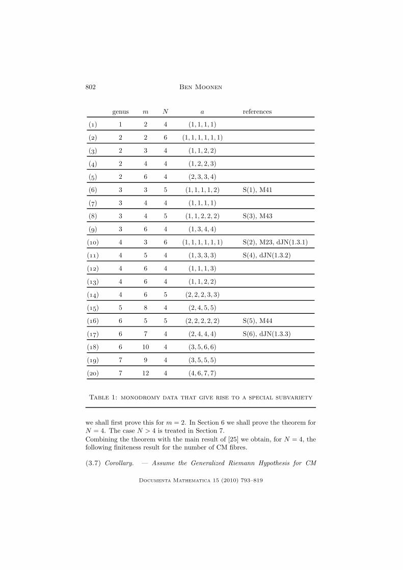
(3.4) Inventory of examples. — Table 1 lists twenty triples (m,N, a) withN > 4 for which N − 3 = dimS(µm), so that Z(m,N, a) ⊂ Ag,C is a specialsubvariety. Our assumption that N > 4 means we are only considering thecases that give rise to a special subvariety of positive dimension.The first column of the table gives a number that we assign to each examplefor reference. The examples are sorted first by genus, then by degree of thecover. The second column gives the genus of the curves in the family. In thenext three columns we give the data (m,N, a). In most cases there is a uniquea = (a1, . . . , aN ) in its equivalence class such that 1 6 a1 6 · · · 6 aN 6 m− 1with

∑

ai = 2m, and if there is a unique such representative, this is the one welist. If N = 4 there are usually two such representatives, the second one being(m− a4,m− a3,m− a2,m− a1); we list the one which lexicographically comesfirst. In the last column we give references to places in the literature where theexample can be found. Here “S(i)” refers to example (i) in [24], “Mi” refersto example i in the appendix of [17], and dJN(1.3.i) refers to example (1.3.i)in [6]. These examples can also be found in [22]; see 4.8 below.

(3.5) Remark. — If we have a triple (m,N, a) as in 2.1 with N = 3, theassociated subvariety Z = Z(m,N, a) is a special point in Ag.

The following theorem is the main result of this paper. It says that the list ofexamples in Table 1 is exhaustive.

(3.6) Theorem. — Consider data (m,N, a) as in 2.1, with N > 4. ThenZ(m,N, a) ⊂ Ag,C is a special subvariety if and only if (m,N, a) is equivalentto one of the twenty examples listed in Table 1.

By what was explained above, it only remains to be shown that Z(m,N, a) isnot special if (m,N, a) is not equivalent to one of the triples in the table. In 4.9


802 Ben Moonen

genus m N a references

() 1 2 4 (1, 1, 1, 1)

() 2 2 6 (1, 1, 1, 1, 1, 1)

() 2 3 4 (1, 1, 2, 2)

() 2 4 4 (1, 2, 2, 3)

() 2 6 4 (2, 3, 3, 4)

() 3 3 5 (1, 1, 1, 1, 2) S(1), M41

() 3 4 4 (1, 1, 1, 1)

() 3 4 5 (1, 1, 2, 2, 2) S(3), M43

() 3 6 4 (1, 3, 4, 4)

() 4 3 6 (1, 1, 1, 1, 1, 1) S(2), M23, dJN(1.3.1)

() 4 5 4 (1, 3, 3, 3) S(4), dJN(1.3.2)

() 4 6 4 (1, 1, 1, 3)

() 4 6 4 (1, 1, 2, 2)

() 4 6 5 (2, 2, 2, 3, 3)

() 5 8 4 (2, 4, 5, 5)

() 6 5 5 (2, 2, 2, 2, 2) S(5), M44

() 6 7 4 (2, 4, 4, 4) S(6), dJN(1.3.3)

() 6 10 4 (3, 5, 6, 6)

() 7 9 4 (3, 5, 5, 5)

() 7 12 4 (4, 6, 7, 7)

Table 1: monodromy data that give rise to a special subvariety

we shall first prove this for m = 2. In Section 6 we shall prove the theorem forN = 4. The case N > 4 is treated in Section 7.

Combining the theorem with the main result of [25] we obtain, for N = 4, thefollowing finiteness result for the number of CM fibres.

(3.7) Corollary. — Assume the Generalized Riemann Hypothesis for CM



fields. If we have a triple (m,N, a) with N = 4 and the equivalence classof this triple is not among the twenty examples listed in Table 1 then up to iso-morphism there are finitely many Jacobians of CM type in the family J → TC.

4. Decomposition of the variation of Hodge structure

In this section we again work over C. We fix a triple (m,N, a) as in 2.1 withN > 4. The corresponding family of curves C → T gives rise to a variation ofHodge structure over T (over C) on whichQ[µm] acts. We describe the resultingdecomposition of the VHS, and we give some results about the monodromy ofthe summands.

(4.1) Let (m,N, a) be as in 2.1. For n ∈ Z/mZ, let N(n) be the number ofindices i ∈ 1, . . . , N such that nai 6≡ 0 modulo m. In particular, N(n) = Nif n ∈ (Z/mZ)∗. If n 6= 0 then dn + d−n = N(n)− 2.Let m′ > 2 be a divisor of m, say with m = rm′. Write N ′ := N(r mod m),and consider the N ′-tuple a′ in (Z/m′Z)N

′

obtained from the N -tuple (a1 modm′, . . . , aN mod m′) by omitting the zero entries. Then (m′, N ′, a′) is again atriple as in 2.1; we refer to it as the triple obtained from (m,N, a) by reductionmodulo m′.

(4.2) As in 2.2, consider the family of curves f : C → T associated with thetriple (m,N, a), where, as in the previous section, we work over C. The coho-mology groups H1(Ct,Q) are the fibres of a polarized Q-VHS with underlyinglocal system V := R1fan

∗ QC . This Q-VHS comes equipped with an action ofthe group ring Q[µm] =

∏

d|mKd, where Kd = Q[t]/Φd is the cyclotomic fieldof dth roots of unity. Accordingly we have a decomposition of Q-VHS,

(4.2.1) V = ⊕d|mV[d] ,

where V[d] is a polarized Q-VHS over T equipped with an action of Kd.

(4.3) Let (m,N, a) be as in 2.1, with N > 4. Let m′ > 2 be a proper divisorof m, and let (m′, N ′, a′) be the triple obtained from (m,N, a) by reductionmodulo m′, as in 4.1.Let ρ: AN → AN ′

be the projection map, omitting the coordinates xi for allindices i with ai ≡ 0 modulo m′. Performing the construction of 2.2 we maychoose T = T (m,N, a) ⊂ AN and T ′ = T (m′, N ′, a′) ⊂ AN ′

such that ρmaps Tto T ′. (The map T → T ′ is then dominant.) If f ′: C′ → T ′ is the family ofcurves associated with the triple (m′, N ′, a′), the pull-back ρ∗C′ = C′×T ′T canbe identified with the quotient of C/T modulo the action of µr ⊂ µm, wherer = m/m′.Let V′ = V(m′, N ′, a′) be the Q-VHS over T ′ associated with the triple(m′, N ′, a′). The quotient morphism C → ρ∗C′ over T gives a map ρ∗V′ → V


804 Ben Moonen

and this induces an isomorphism ρ∗V′ ∼= ⊕d|m′V[d]. We refer to the sub-Q-VHS ρ∗V′ as the old part associated with the divisor m′. The direct summandV[m] ⊂ V is called the new part ; in the decomposition (4.2.1) it is the onlydirect summand that is not contained in an old part.

(4.4) Lemma. — Let the notation and assumptions be as in 4.3. Let g =g(m,N, a) and g′ = g(m′, N ′, a′) be the respective genera. If Z(m,N, a) ⊂ Ag,C

is a special subvariety then Z(m′, N ′, a′) ⊂ Ag′,C is special, too.

Proof. Suppose Z(m,N, a) is special. Write J = J(m,N, a) → T and J ′ =J(m′, N ′, a′) → T ′ for the respective Jacobians. Then ρ∗J ′ is an isogeny factorof J . Hence, if θ: T → Ag′,C is the morphism corresponding to ρ∗J ′, it followsfrom 1.4 that the Zariski closure of the image of θ is a special subvariety. Butθ is just the composition of the projection ρ: T → T ′, which is dominant, andthe morphism φ(m′, N ′, a′): T ′ → Ag′,C associated with the data (m′, N ′, a′).Hence the closure of the image of θ is Z(m′, N ′, a′).

(4.5) With notation as in 2.5, the C-local system VC decomposes as VC =

⊕n∈Z/mZVC,(n). The relation with (4.2.1) is that V[d]C is the sum of all VC,(n)

with ord(n) = d. We have VC,(0) = 0, and for n 6= 0 the C-local system VC,(n)

has rank N(n)− 2, where N(n) is defined as in 4.1. (See also [7], Section 2.)With real coefficients, and with I(m) as in (3.2.1), we have a decomposition ofR-VHS

VR =

⊕

±n∈I(m),2n6≡0

VR,(±n)

⊕ VR,(m

2 ) ,

where the last summand only occurs if m is even. The decomposition is suchthat

VR,(±n) ⊗R C = VC,(n) ⊕ VC,(−n)

andVR,(m

2 ) ⊗R C = VC,(m

2 ) (for even m) .

On the summand VR,(±n) the polarization of the VHS induces a (−1)-hermitianform β±n of signature (dn, d−n); see also [7], Corollary (2.21) and (2.23). Incase m is even, the polarization induces a symplectic form βm

2on VR,(m

2 ).As in 3.3 we choose a base point b ∈ T (C), and a symplectic similitudeσ: H1(Jb,Q)

∼−→ V . Via this similitude, we identify V with the fibre of V

at b. Correspondingly, we write VR,(±n) for the direct summand of VR thatunder σ maps to the fibre at b of VR,(±n).For what follows, it will be convenient to choose the base point b to be a Hodge-generic point with respect to the variation V, so from now on we assume this.Define Mon ⊂ GL(V ) and Hdg ⊂ GL(V ) to be the algebraic monodromy groupsof the Q-local system V and the Hodge group of the fibre at b, respectively.(Since we have chosen b to be Hodge-generic, Hdg is the generic Hodge groupof the VHS.) By [3], Theorem 1, the identity component Mon0 is a semisimplenormal subgroup of Hdg.



(4.6) Remark. — The generic Hodge group Hdg is contained in the algebraicgroup H := GLQ[µm](V )∩CSp(V,Ψ) considered in 3.3. Extending scalars to R

we have

(4.6.1) HR∼=

∏

±n∈I(m),2n6≡0

U(VR,(±n), β±n)

× Sp(VR,(m

2 ), βm

2) ,

where the symplectic factor only occurs ifm is even. Our formula (3.3.1) followsfrom this together with what was explained in 1.5.

We have Mon0 ⊂ Hdg ⊂ H . The next proposition gives us information aboutthe projections of the R-group Mon0R onto the various factors in the decompo-sition (4.6.1).

(4.7) Proposition. — (i) Suppose we have ±n ∈ I(m) with 2n 6≡ 0 such thatdn > 1 and d−n > 1. Then the image of Mon0R in U(VR,(±n), β±n) is the specialunitary group SU(VR,(±n), β±n), which is isomorphic to SU(dn, d−n).

(ii) If m is even, the group Mon0R projects surjectively to the symplectic groupSp(VR,(m

2 ), βm

2), which is isomorphic to Sp2h,R with h = dm

2.

Proof. For (i), see Rohde [22], Theorem 5.1.1. For (ii), assume m is even, andlet h := dm

2. There are then 2h+2 indices i for which ai is even, and without loss

of generality we may assume these are the indices i ∈ 1, . . . , 2h+2. With the

above notation, VR,(m

2 ) is the same as V[2]R , and if we define Mon[2] ⊂ GL(V [2])

as the algebraic monodromy group of the Q-local system V[2] then the image

of Mon0 in Sp(VR,(m

2 ), βm

2) equals Mon

[2],0R . Further, V[2] is just the local system

obtained from the family of hyperelliptic curves u2 = (x − t1) · · · (x − t2h+2);cf. 4.3. By [1], Theorem 1 (see also [2]), the connected algebraic monodromygroup of this local system is the full symplectic group.

(4.8) Let (m,N, a) be a triple as in 2.1, with N > 4. Consider the followingcondition.

(4.8.1)There exists a ±n ∈ I(m) with dn, d−n = 1, N − 3,

and for all other ±n′ ∈ I(m), either dn′ = 0 or d−n′ = 0.

All examples in Table 1, with the exception of Example , satisfy this condition.It has been proven by Rohde in [22] that these nineteen examples are the onlyexamples (up to equivalence) of triples (m,N, a) withN > 4 that satisfy (4.8.1).

(4.9) We now prove Theorem 3.6 for m = 2. In this case N is even, g =(N − 2)/2, and up to equivalence a = (1, . . . , 1) is the only possibility. Further,Z(2, N, a) ⊂ Ag,C is the closure of the hyperelliptic locus in Ag. The assertion isthat this is not special for g > 3. This is true because for g > 3 the hyperellipticlocus is not dense in Ag, whereas by (ii) of Proposition 4.7 the generic Hodgegroup Hdg is the full symplectic group.


806 Ben Moonen

In what follows we may therefore assume m > 2.

5. Canonical liftings of ordinary Jacobiansin positive characteristic

(5.1) We need to recall some definitions and results from the paper [8] byDwork and Ogus. We first discuss their theory in a general setting. After that,from 5.4 on, we return to the specific families of curves that interest us, andwe explain how the results of [8] apply to that situation.Given an irreducible base scheme T and a smooth projective curve f : C → Twe write ωC/T for Ω1

C/T . Consider the Hodge bundle E = E(C/T ) := f∗ωC/T ,which is a vector bundle on T of rank g, the genus of the fibres. We have aKodaira-Spencer map KS: Sym2(E) → Ω1

T/R and we define

K = K (C/T ) := Ker(

Sym2(E)mult−−−→ f∗(ω

⊗2C/T )

)

,

Q = Q(C/T ) := Coker(

f∗(ω⊗2C/T )

∨ mult∨−−−−→ Sym2(E)∨

)

,

where “mult” is the multiplication map. We remark that Q can be thoughtof as the pull-back to T of the normal bundle to the Torelli locus inside Ag.Outside the hyperelliptic locus, mult is surjective and K is the dual of Q.

(5.2) Let k be an algebraically closed field of characteristic p > 0. Consider asmooth projective curve C/k of genus g such that its Jacobian J is ordinary.Let λ be the natural principal polarization of J . By Serre-Tate theory (see [9]or [10], Chap. 5) we have a canonical lifting of (J, λ) to a principally polarizedabelian variety (Jcan, λcan) over the ring of Witt-vectors W (k). In general, forg > 4 this canonical lifting is not the Jacobian of a curve over W (k). Moreprecisely, Dwork and Ogus show that in general not even the canonical liftingover W2(k), the Witt-vectors of length 2, is again a Jacobian.Following [8] we call the ordinary curve C/k pre-W2-canonical if there existsa smooth projective curve Y over W2(k) such that (Jcan, λcan) over W2(k) isisomorphic, as a principally polarized abelian variety, to the Jacobian of Y .The main advantage of working modulo p2 is that in this case there is a naturalclass βC/k in Q(C/k) that vanishes if and only if C/k is pre-W2-canonical; see[8], Prop. (2.4). This invariant βC/k cannot be defined in a family of curves (ina sense that can be made precise, see [8], § 3), but its Frobenius pullback can,as we shall discuss next.Let T be a smooth k-scheme, and let FT : T → T be its absolute Frobeniusendomorphism. Consider a smooth projective curve f : C → T such that allfibres Ct are ordinary. This assumption permits us to view the inverse Cartieroperator as an OT -linear homomorphism

γ: F ∗TE → E ,



with E = E(C/T ) the Hodge bundle. This map γ is the inverse transpose ofthe Frobenius action on R1f∗OC .

Dwork and Ogus define a global section βC/T of F ∗TQ(C/T ) such that for any

t ∈ T (k) the value of βC/T at t is F ∗k (βCt/k). See [8], Prop. 2.7.

The sheaf F ∗TQ(C/T ) comes equipped with a canonical flat connection

∇: F ∗TQ(C/T ) → F ∗

TQ(C/T )⊗ Ω1T/k .

In particular, still with T smooth over k, if Ct/k is pre-W2-canonical for all t ∈T (k), the section βC/T is zero, so certainly ∇βC/T = 0. One of the main points

of [8], then, is that ∇βC/T can be calculated explicitly. The result is easiest tostate under the additional hypothesis that the fibres Ct are not hyperelliptic.We note that this assumption is not always satisfied in the situation we wantto consider. In Prop. 5.8 we shall give a modified version of the next resultthat also works for hyperelliptic families.

If the Ct are not hyperelliptic, the multiplication map Sym2(E) → f∗(ω⊗2) is

surjective, so, with notation as introduced in 5.1, βC/T can be viewed as anOT -linear map F ∗

TK → OT .

The following result is [8], Prop. 3.2. (In [8] the result is stated under some ver-sality assumption on the family C/T but one easily verifies that their Prop. 3.2is true without this assumption.)

(5.3) Proposition (Dwork-Ogus). — With assumptions and notation as above,and assuming the curves Ct to be non-hyperelliptic, −∇(βC/T ): F

∗TK → Ω1

T/k

is equal to the composition

F ∗TK

incl−−→ F ∗

TSym2(E)

Sym2(γ)−−−−−−→ Sym2(E)

KS−−→ Ω1

T/k .

(5.4) Assumptions. — In the rest of this section we fix data (m,N, a) as in 2.1with m > 2 and N > 4, and we consider the family of curves f : C → Tas constructed in 2.2. We assume that (m,N, a) is not equivalent to one ofthe triples listed in Table 1. We further assume that the closed subvarietyZ(m,N, a) ⊂ Ag,C is a special subvariety; our aim is to derive a contradiction.

Without loss of generality we may suppose (m,N, a) is minimal with respectto the above assumptions, by which we mean that there is no triple (m′, N ′, a′)that satisfies our assumptions and for which we have 4 6 N ′ < N or N ′ = Nand 2 6 m′ < m. In particular, it follows from Lemma 4.4 that if m′ is aproper divisor of m and (m′, N ′, a′) is obtained from (m,N, a) by reductionmodulo m′, as in 4.3, either N ′ 6 3 or (m′, N ′, a′) is equivalent to one of thetwenty triples listed in Table 1.


808 Ben Moonen

(5.5) Lemma. — (i) The subsheaf f∗(ω⊗2C/T )(0) of µm-invariant sections of

f∗(ω⊗2C/T ) is a locally free OT -module of rank N − 3.

(ii) The Kodaira-Spencer morphism KS: Sym2(E) → Ω1T/R factors over the

composite map

Sym2(E)pr−−→ Sym2(E)(0)

mult−−−→ f∗(ω

⊗2C/T )(0)

and the induced map KS(0): f∗(ω⊗2C/T )(0) → Ω1

T/R is a fibrewise injective homo-

morphism of vector bundles.

Proof. (i) By a result of Chevalley and Weil in [5], for every t ∈ T (C) thesubspace of µm-invariants in H0(Ct,Ω

⊗2) has dimension N − 3.(ii) The fibre of Sym2(E)(0) at a point t is dual to the space H1(Ct,Θ)(0), whichparametrizes the deformations of Ct for which the µm-action deforms along.Since we have a µm-action on the whole family C/T , the Kodaira-Spencermap factors through the projection Sym2(E) → Sym2(E)(0). For any family

of curves it also factors through the multiplication map Sym2(E) → f∗(ω⊗2C/S);

hence KS factors through f∗(ω⊗2C/T )(0). The last assertion of (ii) just says that

at any t ∈ T (k) our family is complete in the sense of deformation theory: ifD → Spec

(

k[ǫ])

is a first-order deformation of Ct with its µm-action, D/k[ǫ]can be obtained by pull-back from our family. This is clear, as the quotientD/µm is isomorphic to P1

k[ǫ].

(5.6) Lemma. — There exists a prime number p with p ≡ 1 modulo m and,for p a prime of R = Z[1/m, u]/Φm above p, a dense open subset U of T0 :=T ⊗R (R/p), such that for any algebraically closed field k of characteristic p andany t ∈ U(k) the curve Ct is ordinary and the Jacobian Jt is pre-W2-canonical.

Proof. Let p be any prime number with p ≡ 1 mod m. Note that in this caseR/p = Fp for any prime p ⊂ R above p. We write T ⊗ Fp for T ⊗R (R/p). By[4], Prop. 7.4, there is a Zariski open U ⊂ T ⊗ Fp such that Ct is ordinary forall t ∈ U(k). On the other hand, by a theorem of Noot [18], [19], in the slightlymore precise formulation of [13], Thm. 4.2, the assumption that Z = Z(m,N, a)is special implies that for p large enough and t ∈ T0(k) any ordinary point, thecanonical lifting of Jt gives a W (k)-valued point of Z. In particular, Jt is thenpre-W2-canonical.

(5.7) For most choices of (m,N, a) the general member in our family of curvesC → T is not hyperelliptic. In this case we may, and will, choose p and U inLemma 5.6 such that the curves Ct with t ∈ U(k) are non-hyperelliptic.It may happen, however, that Z(m,N, a) is fully contained in the hyperellipticlocus, in which case we call (m,N, a) a hyperelliptic triple. This occurs, forinstance, if m = 2m′ is even and a is of the form (a1, a2,m

′, . . . ,m′), or ifN = 4 and a = (1, 1,m− 1,m− 1). In such a case we will just choose p and Uas in Lemma 5.6.



The following variant of Prop. 5.3 is the essential tool in our proof of Theo-rem 3.6. Let p and U be chosen as above, and let CU → U be the restrictionof C/T to U . With notation as in 2.5 and 5.1 we have eigenspace decompo-sitions Q(CU/U) = ⊕n∈Z/mZ Q(n); likewise for other OU [µm]-modules such as

K (CU/U) and EU = E(CU/U). Accordingly we can write βCU/U =∑

n β(n),

with β(n) a section of F ∗UQ(n).

(5.8) Proposition. — With assumptions and notation as in 5.4 and 5.7, thecomposite map(5.8.1)

F ∗UK(0)

incl−−→ F ∗

USym2(EU )(0)

Sym2(γ)−−−−−−→ Sym2(EU )(0)

mult(0)−−−−−→ f∗(ω

⊗2C/U )(0)

is zero.

Proof. If (m,N, a) is non-hyperelliptic this is immediate from Prop. 5.3 to-gether with (ii) of Lemma 5.5. So from now on we may assume that Z(m,N, a)is contained in the hyperelliptic locus. Let ι ∈ Aut(CU/U) be the hyperellipticinvolution. We remark that ι may or may not be contained in the subgroupµm ⊂ Aut(CU/U); by inspection of the hyperelliptic examples mentioned in 5.7we see that both cases occur.Let ω = Ω1

CU/U . In the hyperelliptic case the multiplication map Sym2(EU ) →

f∗(ω⊗2) is no longer surjective. However, if we denote the invariants under the

action of ι by a subscript “even”,

mult(even): Sym2(EU )(even) → f∗(ω

⊗2)(even)

is again surjective; see for instance [21], Lemmas 2.12 and 2.13. The assump-tion that Z(m,N, a) is fully contained in the hyperelliptic locus implies thatf∗(ω

⊗2)(0) ⊂ f∗(ω⊗2)(even). Hence also mult(0) is surjective, and we may view

β(0) as an OU -linear map F ∗UK(0) → OU .

Our assumptions imply that β(0), hence also ∇β(0), is zero, so all that remainsto be checked is that for the 0-component the analogue of Prop. 5.3 holds.For this we can follow the proof of [8], Prop. 3.2: The proof that loc. cit. dia-gram (3.2.9) is commutative does not use the assumption that the curves arenon-hyperelliptic and therefore goes through in the hyperelliptic case. More-over, in the notation of that proof, we can choose the lifted family Y /T (whereY/T is our CU/U) such that it has an action of µm. Taking 0-componentsin diagram (3.2.9) then gives that −∇β(0) equals the composition of (5.8.1)and KS(0), and by (ii) of Lemma 5.5 we conclude that the map (5.8.1) iszero.

(5.9) Lemma. — Write q = (p − 1)/m. Let n ∈ Z/mZ, and let A = An(t) ∈GLdn

(OU ) be the matrix of the Cartier operator γ−1: EU,(n) → F ∗UEU,(n) with

regard to the frames

ωn,0, . . . , ωn,dn−1 , respectively ωn,0 ⊗ 1, . . . , ωn,dn−1 ⊗ 1 .


810 Ben Moonen

Then the matrix coefficient Aρ,σ, for ρ, σ ∈ 0, . . . , dn − 1, equals

(5.9.1) (−1)Σ ·∑

j1+···+jN=Σ

(

q · [−na1]mj1

)

· · ·

(

q · [−naN ]mjN

)

· tj11 · · · tjNN ,

where Σ = (dn − σ)(p − 1) + (ρ− σ).

Proof. This is the dual version of [4], Lemma 5.1, part (i).

We remark that the result of Bouw in [4] is valid in a more general context. Sheuses this to prove the existence of cyclic covers whose p-rank reaches a naturalupper bound imposed by the local monodromy data; see [4], Thm. 6.1.

6. Proof of the main result: four branch points

In this section we prove Theorem 3.6 in the case N = 4. Let us first try toexplain the idea of the argument, by way of guide for the reader.Assume we have a triple (m,N, a) that is not one of the twenty examples inTable 1 but such that Z(m,N, a) is special. We want to show that this isimpossible. We have the family of curves C → T over a ring R of finite typeover Z; we then consider the reduction modulo p, with p chosen as in 5.7. Thenontrivial information we have, exploiting the assumption that Z(m,N, a) isspecial, is that this gives a family of ordinary Jacobians in characteristic p suchthat the canonical liftings over W2(k) are again Jacobians. In Prop. 5.8 wehave translated this, based on the theory in [8], into the vanishing of a certainabstractly defined map. Lemma 5.9 enables us to calculate this map explicitly.To apply this, we need a differential form that gives us an element in the sourceof the map (5.8.1); we write down such a form in 6.2 below. The fact that theimage of this element is zero then gives us a polynomial identity (6.2.1). Bysome combinatorial arguments we then show that this identity cannot hold if(m,N, a) is not equivalent to one of the twenty special triples in Table 1.

(6.1) We retain the assumptions made in 5.4. In addition we assume N = 4.Let

D(m, a) :=

±n ∈ I(m)∣

∣ dn = d−n = 1

.

(Here I(m) is as defined in (3.2.1) and dn is given by (3.2.2). Though notindicated in the notation, dn depends on a.)If ±n ∈ D(m, a), the equalities dn = d−n = 1 imply that nai 6≡ 0 modulo mfor all i ∈ 1, . . . , 4. Hence,

(6.1.1) [−nai]m = m− [nai]m for all i, and

4∑

i=1

[−nai]m = 2m,

where we recall that [b]m denotes the representative of the class (b mod m) in0, 1, . . . ,m− 1.



We first observe that dimS(µm) > 1. Indeed, if dimS(µm) = 1 then (4.8.1)holds, and by the results of [22], Chapter 6, (m,N, a) is one of the triples inTable 1, which contradicts our assumptions.For n ∈ Z/mZ we have dn + d−n 6 2, and if m is even then dm

26 1. The

inequality dimS(µm) > 1 is therefore equivalent to the fact that #D(m, a) > 2.Choose two distinct pairs ±n and ±n′ in D(m, a). Note that if m is even, wemay have n = −n or n′ = −n′.

(6.2) Choose p and U as in Lemma 5.6, where we may further assume thatthe curves Ct for t ∈ U(k) are either all non-hyperelliptic or all hyperelliptic.We keep the notation introduced in the previous section; in particular we recallthat K (CU/U) = ⊕n∈Z/mZ K(n).It follows from (6.1.1) and the definition of the forms ωn,ν in (2.6.1) that

η := ωn,0 ⊗ ω−n,0 − ωn′,0 ⊗ ω−n′,0

is a section of K(0). For ν ∈ ±n,±n′ the matrix Aν = Aν(t) of Lemma 5.9 isa polynomial in Fp[t1, . . . , t4]. As the Jacobians of the curves Ct for t ∈ U(k)are ordinary, the Cartier operator γ−1 in Lemma 5.9 is an isomorphism ofvector bundles, so Aν(t) is invertible as a section of OU . Because ωn,0 ·ω−n,0 =ωn′,0 · ω−n′,0 is a non-zero section of f∗(ω

⊗2), it follows from Prop. 5.8 that

(6.2.1) An ·A−n = An′ ·A−n′

as polynomials.Define Bν := Aν |t1=0, the polynomial obtained from Aν by substituting t1 = 0.Explicitly,(6.2.2)

Bν = (−1)p−1 ·∑

j2+j3+j4=p−1

(

q · [−νa2]mj2

)

· · ·

(

q · [−νa4]mj4

)

· tj22 tj33 t

j44 .

Fix an index ι ∈ 2, 3, 4, and write 1, 2, 3, 4 = 1, ι ∐ κ, λ. Let vn(ι) bethe largest integer v such that Bn is divisible by tvι . From (6.2.2) and (6.1.1)we find

vn(ι) = max

0, (p− 1)− q · [−naκ]m − q · [−naλ]m

= max

0, q · [naκ]m + q · [naλ]m − (p− 1)

,

and similarly for v−n(ι).Next let w±n(ι) be the largest integer w such that Bn ·B−n is divisible by twι .We find

w±n(ι) = max

0, q · [naκ]m + q · [naλ]m − (p− 1)

+max

0, q · [−naκ]m + q · [−naλ]m − (p− 1)

,

which by (6.1.1) we can rewrite as

(6.2.3)

w±n(ι) = max

0, q · [naκ]m + q · [naλ]m − (p− 1)

+max

0, q · [na1]m + q · [naι]m − (p− 1)

= q ·max

[na1]m + [naι]m, [naκ]m + [naλ]m

− (p− 1) .


812 Ben Moonen

(6.3) Lemma. — Consider two 4-tuples (b1, b2, b3, b4) and (b′1, b′2, b

′3, b

′4) in

1, . . . ,m− 14 with∑4

i=1 bi = 2m =∑4

i=1 b′i. Suppose that for all partitions

1, 2, 3, 4 = 1, ι ∐ κ, λ we have b1 + bι, bκ + bλ = b′1 + b′ι, b′κ + b′λ as

sets. Then there is an even permutation σ ∈ A4 of order 2 such that eitherb′i = bσ(i) for all i or b′i = m− bσ(i) for all i.

Proof. Straightforward checking of all 8 = 23 possible combinations (two foreach partition).

(6.4) The relation (6.2.1) implies that for any partition 1, 2, 3, 4 = 1, ι ∐

κ, λ we have w±n(ι) = w±n′(ι). Since∑4

i=1 [nai]m = 2m =∑4

i=1 [n′ai]m, it

follows from (6.2.3) that

[na1]m + [naι]m, [naκ]m + [naλ]m

=

[n′a1]m + [n′aι]m, [n′aκ]m + [n′aλ]m

as sets. By the lemma it follows, possibly after replacing n by −n, whichwe may do, that there is an even permutation σ ∈ A4 of order 2 such that[n′ai]m = [naσ(i)]m for all i. As the pairs ±n and ±n′ are distinct, σ 6= 1.Possibly after a permutation of the indices we may therefore assume that

(6.4.1)[n′a1]m = [na2]m , [n′a3]m = [na4]m ,

[n′a2]m = [na1]m , [n′a4]m = [na3]m .

Since gcd(m, a1, . . . , a4) = 1 this implies that gcd(m,n) = gcd(m,n′).

(6.5) Let r = gcd(n,m). Let m′ = m/r, and consider the triple (m′, N ′, a′)obtained from (m,N, a) by reduction modulo m′. Then we have a bijectionD(m, a)

∼−→ D(m′, a′) by (±n) 7→ (±n

r ). Hence #D(m′, a′) > 2. In particular,N ′ = 4, and (m′, N ′, a′) is not equivalent to one of the triples listed in Table 1.By our minimality assumption on (m,N, a), see 5.4, it therefore follows thatr = 1. Hence we may replace the 4-tuple a by n′a = (n′a1, . . . , n

′a4), whichmeans we may set n′ = 1 in the above. In this case, (6.4.1) tells us that n2 = 1in (Z/mZ), and the 4-tuple a has the form a = (a1, na1, a3, na3) with n 6= ±1and

(6.5.1) (n+ 1)(a1 + a3) = 2m.

From these relations we want to deduce that there is a pair ±ν ∈ D(m, a) withgcd(m, ν) 6= 1, thereby obtaining a contradiction. Write m = 2k ·M with Modd.First assume n 6≡ −1 modulo M . For an odd prime number ℓ and an exponente > 1, the congruence n2 ≡ 1 mod ℓe only has n ≡ ±1 as solutions. Hencethere is an odd prime divisor ℓ of m such that n 6≡ −1 mod ℓ. But then (6.5.1)gives a1 + a3 ≡ 0 mod ℓ, and since gcd(m, a1, . . . , a4) = 1 we further havea1 6≡ 0 mod ℓ and a3 6≡ 0 mod ℓ. Taking ν := m/ℓ we find that ±ν ∈ D(m, a);contradiction.



The only remaining possibility is that n ≡ −1 modulo M , and therefore n 6≡−1 mod 2k. In particular, k > 2. In this case (6.5.1) implies a1+a3 ≡ 0 mod 4,in which case ±m/4 ∈ D(m, a); contradiction. This completes the proof ofThm. 3.6 in the case N = 4.

7. Proof of the main result: five or more branch points

We now turn to the case N > 5. The idea behind the proof is the sameas in the previous section, but there are some additional difficulties. In 7.2and 7.3 we prove two technical results. Once we have these, we can again writedown elements in the source of the map (5.8.1). Similar to what we did inSection 6, this gives us polynomial identities (7.4.1), and with some elementarycombinatorial arguments we can then conclude the proof.

(7.1) Assumptions. — We retain the assumptions made in 5.4. In addition wenow assume N > 5. Again we assume (m,N, a) is minimal. Because we havealready proven Thm. 3.6 for N = 4, it is again true that ifm′ is a proper divisorofm and (m′, N ′, a′) is obtained from (m,N, a) by reduction modulo m′, eitherN ′ 6 3 or (m′, N ′, a′) is equivalent to one of the twenty triples listed in Table 1.

(7.2) Lemma. — With assumptions as in 7.1, there exists an index n ∈(Z/mZ)∗ such that dn, d−n 6= 0, N − 2.

With the terminology introduced in 4.3, the lemma says that the new part ofthe local system V (as in Section 4) is not isotrivial.

Proof. We assume dn, d−n = 0, N − 2 for all n ∈ (Z/mZ)∗, and weseek to derive a contradiction. It will be convenient to consider the functionδa: Z/mZ → Z>0 given by δa(n) =

∑Ni=1

⟨

−nai

m

⟩

. Note that for n 6= 0 the dndefined in (3.2.2) equals −1 + δa(n). For n ∈ (Z/mZ)∗ we have δa(n) > 1 andδa(n) + δa(−n) = N . Our assumption is equivalent to the condition that

(7.2.1) δa(n), δa(−n) = 1, N − 1 for all n ∈ (Z/mZ)∗.

Possibly after replacing a = (a1, . . . , aN ) by −a, we may assume δa(1) = 1,which means that

(7.2.2) [a1]m + · · ·+ [aN ]m = m.

We divide the proof into a couple of steps.

Step 1. Our first goal is to show thatm > 60. For a givenm, (7.2.2) leaves onlyfinitely many possible triples (m,N, a), up to equivalence. With the help of asmall computer program we check that for m 6 60 the only two possibilitieswith N > 5 and δa(n), δa(−n) = 1, N − 1 for all n ∈ (Z/mZ)∗ are given(up to equivalence) by

(7.2.3) m = 6 , N = 5 , a = (1, 1, 1, 1, 2) ;


814 Ben Moonen

(7.2.4) m = 6 , N = 6 , a = (1, 1, 1, 1, 1, 1) .

So it remains to show that for these triples, Z(m,N, a) is not special.In case (7.2.3), we have g = 7 and the family of Jacobians J → T decomposes,up to isogeny, as a product of three factors: J ∼ Y1 × Y2 × Y3, with— Y1 a pull-back of the Legendre family of elliptic curves, which is Example

in Table 1; this is the old factor corresponding to the divisor 2 of m,— Y2 a pull-back of Example ; this is the old factor corresponding to the

divisor 3 of m,— Y3 the new part.

(The new part Y3 is in fact an isotrivial family of 3-dimensional abelian varietiesof CM type, but we will not need this.) Let b ∈ T (C) be a Hodge-generic point.The fibre Y1,b is an elliptic curve with endomorphism ring Z; its Hodge groupis isomorphic with SL2. The fibre Y2,b is an abelian threefold that is easily seento be simple. (E.g., use the fact that Example is special, together with [23],Thm. 5.) By [16], Prop. 3.8 the Hodge group of Y1,b×Y2,b is the product of thetwo Hodge groups. Hence the smallest special subvariety S ⊂ A7 that containsZ(m,N, a) has dimension at least 1 + 2 = 3 (see 1.5), and since N − 3 = 2 < 3this means that Z(m,N, a) is not special.In case (7.2.4), we have g = 10 and the family of Jacobians J → T decomposes,up to isogeny, as a product of three factors: J ∼ Y1 × Y2 × Y3, with— Y1 a pull-back of Example ; this is the old factor corresponding to the

divisor 2 of m,— Y2 a pull-back of Example ; this is the old factor corresponding to the

divisor 3 of m,— Y3 the new part.

(In this case the new part Y3 is an isotrivial family of 4-dimensional abelianvarieties of CM type; again we will not need this.) For a Hodge-generic pointb ∈ T (C) the fibre Y1,b is an abelian surface with endomorphism ring Z; itsHodge group H1 = Hdg(Y1,b) is isomorphic with Sp4. The fibre Y2,b is anabelian fourfold. By Thm. 1.1 of [26] we have End(Y2,b) = Z[ζ3], and thetangent multiplicities for the factor Y2 (=Example ) are given by d(1 mod 3) =3 and d(2 mod 3) = 1. By [15], 7.4, it follows that for the generic Hodge groupH2 = Hdg(Y2,b) we have H2,R

∼= U(1, 3). If H = Hdg(Jb) is the genericHodge group in our family of Jacobians, H projects surjectively to H1 and H2.It follows that among the simple factors of Had

R both a factor PSp4 and afactor PSU(1, 3) occur; this implies that the smallest special subvariety S ⊂ A7

that contains Z(m,N, a) has dimension at least 3 + 3 = 6 (again see 1.5), andsince N − 3 = 3 < 6 this means that Z(m,N, a) is not special.

Step 2. The function δa has the property that δa(n1 + n2) 6 δa(n1) + δa(n2).In particular, if n1, n2 and n1 + n2 are all in (Z/mZ)∗ then by (7.2.1) we havethe implication

(7.2.5) δa(n1) = δa(n2) = 1 ⇒ δa(n1 + n2) = 1 .



Step 3. Next we show that m is not divisible by 2, 3 or 5. Let p ∈ 2, 3, 5,and suppose m is divisible by p. Let m′ = m/p and let (m′, N ′, a′) be obtainedfrom (m,N, a) by reduction modulo m′. The new triple cannot be one of theexamples listed in Table 1, for this would imply (by inspection of the table)that m = p ·m′ 6 5 · 12 = 60, which we have excluded. Hence our minimalityassumption on the triple (m,N, a) implies that N ′ 6 3.Since N > 5, there are at least two indices i such that ai ≡ 0 modulo m′. Forp = 2 this contradicts (7.2.2). Hence 2 ∈ (Z/mZ)∗ and by repeated applicationof (7.2.5), starting from δa(1) = 1, we find that δa(2

k) = 1 for all k.For p = 3 the only possibility left, in view of (7.2.2), is that there are preciselytwo indices i with [ai]m = m/3 and that [ai]m < m/3 for all remaining indices.This contradicts the fact that δa(2) = 1. Hence 3 does not divide m.Finally take p = 5. The fact that δa(2) = 1 implies that there is a uniqueindex i with [ai]m > m/2 and that [ai]m < m/2 for all remaining indices.Since N > 5 and N ′ 6 3 this leaves (possibly after a permutation of theindices) two possibilities: either

[a1]m = 3m/5 , [a2]m = m/5 , [ai]m < m/5 for all i > 2,

or

m/2 < [a1]m < 3m/5 , [a2]m = [a3]m = m/5 , [ai]m < m/5 for all i > 3.

In both cases we get a contradiction with the fact that δa(4) = 1.

Step 4. We now show that m has at most four distinct prime divisors. Tosee this, let p be any prime divisor of m, let m′ = m/p and let (m′, N ′, a′) beobtained from (m,N, a) by reduction modulo m′. If the new triple is one of theexamples listed in Table 1, it can only be Example , for otherwise inspectionof the table gives that m′ (and hence m) is divisible by 2, 3, or 5, which wehave excluded. Example has N ′ = 4 branch points, so this fact, togetherwith our minimality assumption on the triple (m,N, a), implies that N ′ 6 4.The previous argument shows that for any prime divisor p of m, there are atmost 4 indices i such that ai is not divisible by m/p. On the other hand,ai 6≡ 0 mod m, so for a given index i there can be at most one prime divisor pof m such that ai is divisible by m/p. As N > 5 it follows that m has at mostfour distinct prime divisors.

Step 5; conclusion of the proof. Combining the conclusion of Step 3 with (7.2.5),we find that for all ρ ∈ 1, 2, 3, 4, 5 we have (ρ mod m) ∈ (Z/mZ)∗ andδa(ρ mod m) = 1.Let ν be an integer such that gcd(m, ν) = 1 and δa(ν mod m) = 1. Let ρ bethe smallest positive integer such that gcd(m, ν + ρ) = 1. The fact that mhas at most four distinct prime divisors, all greater than 5, implies that ρ 6 5.But then gcd(ρ,m) = 1 and from (7.2.5) we get that δa(ν + ρ mod m) = 1.Repeating this, we find that δa(n) = 1 for all n ∈ (Z/mZ)∗, which contradictsthe fact that δa(n) + δa(−n) = N > 3. This completes the proof of thelemma.


816 Ben Moonen

(7.3) Our next goal is to show there exist two distinct pairs ±n and ±n′

in I(m) with

(7.3.1) d−n = d−n′ = 1 , and dn = dn′ = N − 3 .

(In particular, n 6≡ 0 and n′ 6≡ 0.) For this we work over C and we considerthe generic Mumford-Tate group M of the family C/T . As in 1.5, let Mad

R =Q1 × · · · × Qr be the decomposition of Mad

R as a product of simple factors.The assumption that Z(m,N, a) is special means that N − 3 =

∑ri=1 d(Qi),

with notation as in 1.5. Further, this assumption implies that the connectedalgebraic monodromy group Mon0 of the family is a normal subgroup of M ; inparticular, Mon0,adR =

∏

i∈K Qi for some subset K ⊂ 1, . . . , r.By Lemma 7.2 there exists an index n in (Z/mZ)∗ with dn, d−n 6= 0, N −2. By Prop. 4.7 it follows that one of the simple factors Qi, say Q1, is aPSU(dn, d−n), which gives d(Q1) = dnd−n. Because n ∈ (Z/mZ)∗ we havedn+d−n = N−2; hence dnd−n > N−3 with equality of and only if dn, d−n =1, N − 3. Possibly after replacing n by −n we therefore have dn = N − 3and d−n = 1. Further, the relation N − 3 =

∑ri=1 d(Qi) implies that all other

simple factors Q2, . . . , Qr are anisotropic (i.e., compact).Our assumptions imply that there is another index pair ±n′ ∈ I(m) withdn′ 6= 0 and d−n′ 6= 0, for if this is not the case then (m,N, a) satisfies (4.8.1),which implies it is one of the examples of Table 1. If m = 2m′ is even andn′ = m′ then by Prop. 4.7 one of the factors Qi is a PSp2h with h = dn′ > 0.As N − 3 > 2, this factor cannot be the factor Q1 = PSU(1, N − 3), and sincePSp2h is not anisotropic we arrive at a contradiction. So n′ 6= −n′, and, againby Prop. 4.7, one of the Qi is a non-compact unitary factor PSU(dn′ , d−n′).This factor must be the factor Q1; hence dn′ , d−n′ = 1, N − 3, which giveswhat we want.

(7.4) Consider two distinct pairs ±n and ±n′ in I(m) for which (7.3.1) holds.Let Γ ∈ GLN−3(OU ) be the matrix of γ(n): F

∗UEU,(n) → EU,(n) with regard to

the frames given by the forms ωn,σ. It is the inverse of the matrix A = An ofLemma 5.9. Similarly, let Γ′ be the matrix of γ(n′), and let A′ = An′ be itsinverse. Further, let c and c′ be the sections of O∗

U (the inverses of the 1 × 1matrices A−n and A−n′ of Lemma 5.9) such that γ(ω−n,0 ⊗ 1) = c · ω−n,0 andγ(ω−n′,0 ⊗ 1) = c · ω−n′,0.For σ ∈ 0, 1, . . . , N − 4, let ησ ∈ Γ(U,K(0)) be given by

ησ := ω−n,0 ⊗ ωn,σ − ω−n′,0 ⊗ ωn′,σ .

As ω−n,0 · ωn,ρ = ω−n′,0 · ωn′,ρ as sections of f∗(ω⊗2), the image of ησ un-

der Sym2(γ) equals

N−4∑

ρ=0

(

c · Γρ,σ − c′ · Γ′ρ,σ

)

· (ω−n,0 · ωn,ρ) .



Because the sections ω−n,0 ·ωn,ρ for ρ ∈ 0, . . . , N−4 are linearly independent,it follows from Prop. 5.8 that c · Γρ,σ − c′ · Γ′

ρ,σ for all σ, ρ ∈ 0, 1, . . . , N − 4,which can be rewritten as

(7.4.1) c−1 ·Aρ,σ = c′,−1 · A′ρ,σ .

Choose two distinct indices κ, λ in 1, 2, . . . , N, and write 1, . . . , N =κ, λ ∐ I. For ν ∈ 0, 1, define vn(ν) to be the largest integer v such thatAν,ν |tκ=0 is divisible by tvλ. Similarly, let v−n be the largest integer v such thatc−1|tκ=0 is divisible by t

vλ. Using the explicit formulas for c−1 and the matrix A

from Lemma 5.9, we find

v−n = max

0, (p− 1)− q ·∑

i∈I

[nai]m

,

vn(0) = max

0, (N − 3)(p− 1)− q ·∑

i∈I

[−nai]m

,

vn(1) = 0 .

(Recall that q = (p− 1)/m.)Next we define wn(ν) = v−n + vn(ν) to be the largest integer w such that(

c−1 · Aν,ν

)

|tκ=0 is divisible by twλ . Similar to (6.1.1), it follows from the factthat d−n = 1 and dn = N − 3 that [−nai]m = m − [nai]m for all i and∑N

i=1 [nai]m = 2m. Using these relations we obtain

w(0) = max

(p− 1)− q ·∑

i/∈I

[nai]m, (p− 1)− q ·∑

i∈I

[nai]m

=∣

∣

∣(p− 1)− q ·∑

i/∈I

[nai]m

∣

∣

∣ = q ·∣

∣m− [naκ]m − [naλ]m∣

∣ ,

w(1) = max

0, (p− 1)− q ·∑

i∈I

[nai]m

= max

0, (p− 1)− q ·∑

i/∈I

[nai]m

= q ·max

0, [naκ]m + [naλ]m −m

.

We can do the same calculations for the pair ±n′; let us call w′(0) and w′(1)the resulting values. From (7.4.1) we get the relations w(0) = w′(0) andw(1) = w′(1). It follows that for all choices of κ and λ we have [naκ]m +[naλ]m = [n′aκ]m + [n′aλ]m. This readily implies that [nai]m = [n′ai]m for alli ∈ 1, . . . , N. As gcd(m, a1, . . . , aN ) = 1 it follows that n = n′, which contra-dicts our assumption that the pairs ±n and ±n′ are distinct. This completesthe proof of Theorem 3.6.


818 Ben Moonen

References

[1] N. A’Campo, Tresses, monodromie et le groupe symplectique. Comment.Math. Helv. 54 (1979), 318–327.[2] J. Achter, R. Pries, The integral monodromy of hyperelliptic and triellipticcurves. Math. Ann. 338 (2007), 187–206.[3] Y. Andre,Mumford-Tate groups of mixed Hodge structures and the theoremof the fixed part. Compositio Math. 82 (1992), 1–24.[4] I. Bouw, The p-rank of ramified covers of curves. Compositio Math. 126(2001), 295–322.[5] C. Chevalley, A. Weil, Uber das Verhalten der Integrale 1. Gattung beiAutomorphismen des Funktionenkorpers. Abh. Math. Semin. Univ. Hambg. 10(1934), 358–361.[6] J. de Jong, R. Noot, Jacobians with complex multiplication. In: Arithmeticalgebraic geometry (Texel, 1989), Progr. Math. 89, Birkhauser, 1991, pp. 177–192.[7] P. Deligne, G. Mostow, Monodromy of hypergeometric functions and non-lattice integral monodromy. Inst. Hautes Etudes Sci. Publ. Math. 63 (1986),5–89.[8] B. Dwork, A. Ogus, Canonical liftings of Jacobians. Compositio Math. 58(1986), 111–131.[9] N. Katz, Serre-Tate local moduli. In: Algebraic surfaces, Lecture Notes inMath. 868, Springer-Verlag, 1981, pp. 138–202.[10] W. Messing, The crystals associated to Barsotti-Tate groups: with appli-cations to abelian schemes. Lecture Notes in Math. 264, Springer-Verlag, 1972.[11] B. Moonen, Special points and linearity properties of Shimura varieties.PhD thesis, University of Utrecht, 1995.[12] B. Moonen, Linearity properties of Shimura varieties. I. J. Alg. Geom. 7(1998), 539–567.[13] B. Moonen, Linearity properties of Shimura varieties. II. CompositioMath. 114 (1998), 3–35.[14] B. Moonen, F. Oort, The Torelli locus and special subvarieties. Preprint,August 2010, 43pp.[15] B. Moonen, Yu. Zarhin, Hodge classes and Tate classes on simple abelianfourfolds. Duke Math. J. 77 (1995), 553–581.[16] B. Moonen, Yu. Zarhin, Hodge classes on abelian varieties of low dimen-sion. Math. Ann. 315 (1999), 711–733.[17] G. Mostow, On discontinuous action of monodromy groups on the complexn-ball. J. Amer. Math. Soc. 1 (1988), 555–586.[18] R. Noot, Hodge classes, Tate classes, and local moduli of abelian varieties.PhD thesis, University of Utrecht, 1992.[19] R. Noot, Models of Shimura varieties in mixed characteristic. J. Alg.Geom. 5 (1996), 187–207.[20] R. Noot, Correspondances de Hecke, action de Galois et la conjectured’Andre-Oort (d’apres Edixhoven et Yafaev). Sem. Bourbaki, Exp. 942.



Asterisque 307 (2006), 165–197.[21] F. Oort, J. Steenbrink, The local Torelli problem for algebraic curves. In:Journees de Geometrie Algebrique d’Angers, Sijthoff & Noordhoff, 1980, pp.157–204.[22] J. Rohde, Cyclic coverings, Calabi-Yau manifolds and complex multiplica-tion. Lecture Notes in Math. 1975, Springer, 2009.[23] G. Shimura, On analytic families of polarized abelian varieties and auto-morphic functions. Ann. of Math. (2) 78 (1963), 149–192.[24] G. Shimura, On purely transcendental fields of automorphic functions ofseveral variable. Osaka J. Math. 1 (1964), 1–14.[25] A. Yafaev, A conjecture of Yves Andre’s. Duke Math. J. 132 (2006), 393–407.[26] Yu. Zarhin, The endomorphism rings of Jacobians of cyclic covers of theprojective line. Math. Proc. Cambridge Philos. Soc. 136 (2004), 257–267.

Ben MoonenUniversity of AmsterdamKdV Institute for MathematicsPO Box 942481090 GE AmsterdamThe Netherlands


820

Documenta Mathematica 15 (2010)

specialsubvarieties arisingfrom families of cyclic covers ... · specialsubvarieties arisingfrom...

Documents