Spectral Analysis of Stochastic Processes

Henning Rust

hrust@uni-potsdam.de

Nonlinear Dynamics Group, University of Potsdam

Lecture Notes for the

E2C2 / GIACS Summer School,

Comorova, Romania

September 2007

2

Chapter 1

Time Series Analysisand Stochastic Modelling

A time series is a sequence of data points measured at successive time intervals. Un-derstanding the mechanism that generated this time series or making predictions are theessence of time series analysis. Applications range from physiology (e.g., ?) and systemsbiology (e.g., ?), over economy (e.g., ?) and geophysical problems as daily weather fore-casts (e.g., ?) or detection and prediction of climate change (e.g., ?) to astronomy (e.g.,?).

This chapter introduces some concepts of linear time series analysis and stochasticmodelling. Starting with random variables, we briefly introduce spectral analysis anddiscuss some special stochastic processes. An emphasis is made on the difference be-tween short-range and long-range dependence, a feature especially relevant for trenddetection and uncertainty analysis. Equipped with a canon of stochastic processes, wepresent and discuss ways of estimating optimal process parameters from empirical data.

1.1 Basic Concepts of Time Series Analysis

1.1.1 Random Variables

A random variable X is a mapping X : Ω → R from a sample space Ω onto the real axis.Given a random variable one can define probabilities of an event. As a simple examplewe consider a die with a sample space Ω = 1, 2, 3, 4, 5, 6. The probability P for theevent d ∈ Ω, d =“the number on a die is smaller than 4” is denoted as P(X < 4). Suchprobabilities can be expressed using the cumulative probability distribution function

FX(x) = P(X ≤ x). (1.1)

For a continuous random variable X, FX(x) is continuous. A discrete random variable Xleads to FX(x) being a step function.

With miniscules x we denote a realisation x ∈ R, a possible outcome of a randomvariable X. A sample is a set of N realisations xii=1,...,N .

Dependence

Two random variables X and Y are independent if their joint probability distribution P(X <

x, Y < y) can be written as a product of the individual distributions: P(X < x, Y < y) =

3

P(X < x)P(Y < y), or, using the conditional distribution, P(X < x | Y < y) = P(X < x).They are called dependent otherwise. A particular measure of dependence is the covari-ance which specifies the linear part of the dependence:

cov(X, Y) = E [(X − E [X])(Y − E [Y])] , (1.2)

where E [X] =∫

Rx fX(x)dx denotes the expectation value with fX(x) = dFX(x)/dx be-

ing the probability density function (?).A normalised measure quantifying the strength and direction1 of the linear relation-

ship of two random variables X and Y is the correlation

cor(X, Y) =cov(X, Y)√

var(X)√

var(Y), (1.3)

with var(X) = cov(X, X) being the variance of X. It is a normalised measure tak-ing values in the interval −1 ≤ cor(X, Y) ≤ 1. An absolute correlation of unity, i.e.|cor(X, Y)| = 1, implies Y being a linear function of X.

The variables X and Y are said to be uncorrelated if their covariance function, andthus their correlation, vanishes:

cov(X, Y) = 0. (1.4)

Correlated random variables are also dependent. The opposite statement is not neces-sarily true, because the correlation captures only the linear part of the dependence. In-dependent random variables Xi with identical distribution function are referred to asindependent and identically-distributed random variables (IID).

For a set of random variables X1, X2, . . . , XM the covariance matrix Σ with elementsΣij is defined as

Σij = cov(Xi, Xj). (1.5)

1.1.2 Stochastic Processes

The word stochastic originates from the Greek stochazesthai (στωχαξǫσθαι) meaning “toaim at” or “to guess at” (?). It is used in the sense of random in contrast to deterministic.While in a deterministic model the outcome is completely determined by the equationsand the input (initial conditions), in a stochastic model no exact values are determinedbut probability distributions. In that sense, a stochastic model can be understood as ameans to guess at something.

The choice between a deterministic and a stochastic model is basically one of whatinformation is to be included in the equations describing the system. On the one handinformation can be limited simply by the lack of knowledge. On the other hand it mightnot be benefitting the modelling objective to include certain information.

A stochastic process X(t) or Xt is an indexed collection of random variables withthe indices specifying a time ordering. The index set can either be discrete (t ∈ N) orcontinuous (t ∈ R). In the latter case the collection consists of an uncountable infinitenumber of random variables.

With xt=1,...,N = (x1, x2, . . . , xN) we denote a realisation of the stochastic process Xt

for 1 ≤ t ≤ N. Where unambiguous, we omit the index. Depending on the context, x

also denotes an empirical data record which is considered as a realisation of a possiblyunknown process.

1Direction specifies the sign of the correlation. The direction is positive if X increases when Y increasesand negative otherwise. It is not meant in the sense of variable X influencing variable Y or vice versa.

4

Stationarity

If the joint probability distribution P(Xt1< x1, Xt2 < x2, . . . , Xtn < xn), with ti ∈ N, is

identical with a displaced one P(Xt1+k < x1, Xt2+k < x2, . . . , Xtn+k < xn) for any admissi-ble t1, t2, . . . , tn and any k, the process is called completely stationary.

An alleviated concept is stationarity up to an order m with the first m moments of thejoint probability distribution existing and being equal to those of the displaced one. Forpractical applications, frequently stationarity up to order m = 2 or weak stationarity isrequired. Testing for higher orders or for complete stationarity is usually not feasible.

Autocovariance

The covariance of two instances Xt1and Xt2 at two different times t1 and t2 of a stochastic

process Xt is called autocovariance

cov(Xti, Xtj

) = E[(

Xti− E

[Xti

] )(Xtj

− E[

Xtj

] )]. (1.6)

For processes which are stationary at least up to order m = 2 the autocovariance dependsonly on the differences τ = ti − tj and can be written as

cov(τ) = E[(

Xt − E [Xt])(

Xt+τ − E [Xt])]

. (1.7)

Analogously, the autocorrelation can be defined as

ρ(Xti, Xtj

) =cov(Xti

, Xtj)

√var(Xti

)√

var(Xtj)

, (1.8)

and in case of at least weak stationarity it can be written as

ρ(τ) = ρ(Xt, Xt+τ). (1.9)

In the following, we refer to Equation (1.9) as the autocorrelation function or ACF.

Given a sample of an unknown process, we can estimate process characteristics as theACF. An estimator for a characteristic T is a function of the sample and will be denotedby T. A nonparametric estimate for the autocovariance of a zero mean record xt=1,...,N isthe sample autocovariance function or autocovariance sequence (?)

cov(τ) =1

N

N−τ

∑t=1

xtxt+τ , 0 ≤ τ < N. (1.10)

Using the divisor N instead of N − τ ensures that the estimate for the autocovariance ma-trix Σ is non-negative definite. Consequently an estimate for the autocorrelation functioncan be formulated as

ρ(τ) =cov(τ)

σ2x

, (1.11)

with σ2x = cov(0) being an estimate of the record’s variance.

The estimator is asymptotically normal and the variance can be approximated byρ(τ) = n−1, a 95% confidence interval is thus given by [−1.96n−1, 1.96n−1] (?).

For a more detailed description of these basic concepts refer to, e.g., ??, or ?.

5

1.1.3 Spectral Analysis

While the time domain approach to time series analysis originates from mathematicalstatistics, the spectral or frequency domain approach has its root in communication engi-neering. Whenever a signal fluctuates around a certain stable state we might use periodicfunctions to describe its behaviour. Spectral analysis aims at splitting the total variabilityof a stationary stochastic process into contributions related to oscillations with a certainfrequency.

For the definition of the spectral density of a continuous stationary process X(t) con-sider initially the process

XT(t) =

X(t), if − T ≤ t ≤ T0, otherwise

. (1.12)

This process is absolutely integrable due to the compact support [−T, T]. We now candefine a Fourier integral as

GT(ω) =1√2π

∫ T

−TXT(t)e−iωtdt. (1.13)

and a power spectral density

S(ω) = limT→∞

|GT(ω)|22T

. (1.14)

We use the notion of power as energy per time to obtain a finite spectral density. The aimis to represent the stochastic process and not only a single realisation. We thus have toaverage over multiple realisations. This leads us to a definition of a power spectral densityfor stochastic processes

S(ω) = limT→∞

E

[ |GT(ω)|22T

]. (1.15)

In the following, we refer to the power spectral density simply as the spectral density. Adetailed derivation of this concept is given by ?.

Relation to the Autocovariance

The relation between the spectral density S(ω) and the autocovariance function cov(τ) ofa zero mean process is surprising at first sight. Using some basic properties of the Fouriertransform, we can establish that the spectral density can be expressed as the Fourier trans-form of the autocovariance function:

S(ω) =1

2π

∫ ∞

−∞cov(τ)e−iωτdτ. (1.16)

In a more general setting, when the spectral density function does not exist but the inte-grated spectrum F(ω) does, this result manifests in the Wiener-Khinchin theorem usingthe more general Fourier-Stieltjes form of the integral (?)

ρ(τ) =∫ ∞

−∞eiωτdF(ω), (1.17)

with ρ(τ) being the ACF. Thus, the spectral density and the ACF are equivalent descrip-tions of the linear dynamic properties of a process.

6

Estimation of the Spectral Density

Given a zero mean series x sampled at discrete time points t = 1, . . . , N, an estimator forthe spectral density function (1.15) can be formulated using the periodogram I(ωj)

S(ωj) = I(ωj) =1

2πN|

N

∑t=1

xte−itωj|2, (1.18)

with the Fourier frequencies ωj = 2πj/N and j = 1, . . . , [(N − 1)/2], where [.] denotesthe integer part. The largest frequency to be resolved is the Nyquist frequency fNy =

12π ωNy = 2π

2∆, where ∆ is the sampling interval.

The periodogram is not a consistent2 estimator for the spectral density because itsvariance does not decrease with increasing length N of the sample. To obtain a consistentestimator we can locally smooth the periodogram with, e.g., a suitable rectangular orbell-shaped window (e.g., ?).

For Gaussian stochastic processes, the periodogram I(ωj) at a certain angular fre-quency ωj is χ2-distributed with two degrees of freedom: I(ωj) ∼ χ2

2. This result allowsto derive confidence intervals for the power at a certain frequency (?).

Instead of the angular frequency ω, it is convenient to use the frequency f = ω/2πin practical applications. In this way, we can specify frequencies as reciprocal periods,which are expressed in units of the sampling interval, e.g., 1/days for data with a dailyresolution.

1.1.4 Long-Range Dependence

For some stochastic processes, such as the popular autoregressive and moving averagetype models that will be introduced in Section 1.2, the ACF, denoted as ρSRD(τ), decaysexponentially and is thus summable:

∞

∑τ=−∞

ρSRD(τ) = const < ∞. (1.19)

These processes are called short-range dependent (SRD) or short-range correlated.This characteristic contradicted other findings from, e.g., a spatial analysis of agricul-

tural data by ? or the famous Nile River flow minima studied by ?. The behaviour theyobserved for the ACF for large lags – often referred to as Hurst phenomenon – was notconsistent with hitherto existing models describing dependence. It was well representedassuming an algebraic decay of the ACF: ρLRD(τ) ∝ τ−γ. This type of decay leads to adiverging sum

∞

∑τ=−∞

ρLRD(τ) = ∞. (1.20)

Processes with an ACF following (1.20) are called long-range dependent (LRD), long-rangecorrelated or long-memory processes.

Alternative Definitions of Long-Range Dependence

0 Today, it is common to use equation (1.20) as definition for a long-range dependentprocess (?). The following alternative formulations in the time and spectral domain, re-spectively, are consistent with (1.20).

2An estimator TN for the parameter T based on N observations is consistent iff for all ǫ > 0

limN→∞ P((TN − T) < ǫ) = 1.

7

Time Domain Let Xt be a stationary process. If there exists a real number γ ∈ (0, 1)and a constant cρ > 0 such that

limτ→∞

ρ(τ)

τ−γ= cρ (1.21)

holds, then Xt is called a process with long-range dependence or long memory.

Spectral Domain If there exists a real number β ∈ (0, 1) and a constant c f > 0 such that

limω→0

S(ω)

|ω|−β= cS (1.22)

holds then Xt is called a process with long-range dependence.The concept of long-memory refers to non-periodic stochastic processes. Therefore

the recurrence due to periodicities, such as the Milankovitch cycles3 in the climate system,is not to be considered as long-range dependence, even if their (deterministic) behaviourcauses dependence for infinite time lags.

1.2 Some Stationary Stochastic Processes

This section introduces some examples of stationary stochastic processs, SRD, as wellas LRD processes. They can be used to describe e.g. temperaure anomalies or run-offrecords.

Gaussian Processes

A stochastic process Xt with joint probability distribution P(Xt1< x1, Xt2 < x2, . . . , Xtk

<

xk) for all tk ∈ N being multivariate normal is called a Gaussian process. It is completelydefined by its first two moments, the expectation value E [Xt] and the autocovariancefunction cov(Xti

, Xtj) or autocovariance matrix Σ. This implies that a weakly stationary

Gaussian process is also completely stationary (cf. Section 1.1.2). Furthermore, a Gaus-sian process is thus a linear process, because the autocovariance matrix specifies only lin-ear relationships between the different instances Xtk

. Simple examples for discrete timeGaussian stochastic processes are the Gaussian white noise and autoregressive processesdescribed in the following.

1.2.1 Processes with Short-Range Dependence

Gaussian White Noise Process

Let Xtt=0,±1,±2,... be a sequence of uncorrelated4 Gaussian random variables, then Xt

is called a Gaussian white noise process or a purely random process. It possesses “nomemory” in the sense that the value at time t is not correlated with a value at any othertime s: cov(Xt, Xs) = 0, ∀t 6= s. Hence, the spectrum is flat. A plot of a realisation andthe corresponding periodogram of a zero mean Gaussian white noise process is given inFigure 1.1. In the following, we frequently refer to a Gaussian white noise process simplyas white noise. To state that Xt is such a process with mean µ and variance σ2, we use thenotation Xt ∼ WN (0, 1).

3Milankovitch cycles are quasi-periodic changes in the earth’s orbital and rotational properties resultingfrom being exposed to the gravitational force of multiple planets. The change in the orbital parameters effectthe earth’s climate.

4or, more generally, independent

8

0 100 200 300 400 500

−4

−2

02

4

t

X

0.0 0.5 1.0 1.5 2.0 2.5 3.0

0.00

10.

050

1.00

0

Po

wer

ω

Figure 1.1: Realisation of a white noise process with 500 points (left) and the corresponding peri-odogram with the spectral density as red solid line (right).

First Order Autoregressive Process (AR[1])

An instance Xt at time t of an autoregressive process depends on its predecessors in alinear way. A first order autoregressive process (AR[1]), depends thus only on its lastpredecessor and it includes a stochastic noise or innovations term ηt in the following way:

Xt = aXt−1 + ηt. (1.23)

If not explicitely stated otherwise, we assume throughout this thesis the driving noiseterm ηt to be a zero mean Gaussian white noise process with variance σ2

η : ηt = WN (0, σ2η).

A discussion for non-zero mean noise terms can be found in ?. If ηt is Gaussian then theAR process is completely specified by its second order properties. Those are in turn de-termined by the propagator a and the variance σ2

η of η. Figure 1.2 shows a realisation andthe corresponding periodogram of an AR[1] process.

0 100 200 300 400 500

−4

−2

02

4

t

X

0.0 0.5 1.0 1.5 2.0 2.5 3.0

1e−

031e

−01

1e+

01

Po

wer

ω

Figure 1.2: Realisation of an AR[1] process with 500 points (left) and the corresponding peri-odogram with the spectral density as red solid line (right). The autoregressive parameter is set toa = 0.7.

9

Mean and Autocovariance function Assuming X0 = 0 the derivation of the mean andautocovariance function for this process is straightforward. Iteratively using (1.23) yields

Xt = aXt−1 + ηt

= a(aXt−2 + ηt−1) + ηt

...

= at−1η1 + at−2η2 + · · · + a2ηt−2 + aηt−1 + ηt. (1.24)

Taking expectation values on both sides and using E [ηt] = 0 yields E [Xt] = 0. Using thisresult, the autocovariance function for τ ≥ 0 is

cov(Xt, Xt+τ) = E[(at−1η1 + at−2η2 + · · · + ηt)(at+τ−1η1 + at+τ−2η2 + · · · + ηt+τ)

]

= σ2η (a2(t−1)+τ + a2(t−2)+τ + · · · + aτ)

=

σ2

η t, if|a| = 1

σ2η aτ

(1−a2t

1−a2

), else.

(1.25)

Stationarity Setting |a| < 1 leads to cov(Xt, Xt+τ) being asymptotically (i.e. for large t)independent of t and thus the process is called asymptotically stationary. For a = 1 weobtain a non-stationary process, i.e. with X0 = 0

Xt = Xt−1 + ηt = Xt−2 + ηt−1 + ηt = · · · =t

∑i=0

ηi . (1.26)

This process is known as the random walk (?). In the limit of small step sizes, the randomwalk approximates Brownian motion.

Higher Order Autoregressive Processes (AR[p])

The autoregression in (1.23) can be straightforwardly extended to include more regressorswith larger time lags. A general definition of an AR[p] process with p regressors is

Xt =p

∑i=1

aiXt−i + ηt, (1.27)

with ηt ∼ WN (0, ση) being white noise. Rearranging the terms and using the back-shiftoperator BXt = Xt−1, (1.27) reads

(1 − a1B − a2B2 − · · · − apBp)Xt = ηt. (1.28)

It is convenient to define the autoregressive polynomial of order p

Φ(z) = (1 − a1z − a2z2 − · · · − apzp). (1.29)

Now, (1.27) reads simplyΦ(B)Xt = ηt. (1.30)

Deriving the condition for asymptotic stationarity of an AR[p] process is somewhat moreintricate. It leads to investigating whether the roots of Φ(z), with z ∈ C, lying outside theunit circle of the complex plane (cf. ??).

10

The general form of the autocorrelation function is given by

ρ(τ) = A1φ|τ|1 + A2φ

|τ|2 + · · · + Apφ

|τ|p , (1.31)

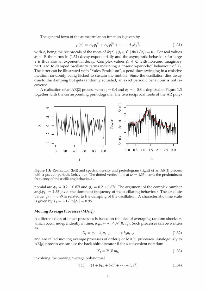
with φi being the reciprocals of the roots of Φ(z):φi ∈ C | Φ(1/φi) = 0. For real valuesφi ∈ R the terms in (1.31) decay exponentially and the asymptotic behaviour for largeτ is thus also an exponential decay. Complex values φi ∈ C with non-zero imaginarypart lead to damped oscillatory terms indicating a “pseudo-periodic” behaviour of Xt.The latter can be illustrated with “Yules Pendulum”, a pendulum swinging in a resistivemedium randomly being kicked to sustain the motion. Since the oscillation dies awaydue to the damping but gets randomly actuated, an exact periodic behaviour is not re-covered.

A realisation of an AR[2] process with a1 = 0.4 and a2 = −0.8 is depicted in Figure 1.3together with the corresponding periodogram. The two reciprocal roots of the AR poly-

0 20 40 60 80 100

−4

−2

02

4

t

X

0.0 0.5 1.0 1.5 2.0 2.5 3.0

5e−

035e

−01

5e+

01

Po

wer

ω

Figure 1.3: Realisation (left) and spectral density and periodogram (right) of an AR[2] processwith a pseudo-periodic behaviour. The dotted vertical line at ω = 1.35 marks the predominantfrequency of the oscillating behaviour .

nomial are φ1 = 0.2 − 0.87i and φ2 = 0.2 + 0.87i. The argument of the complex numberarg(φ1) = 1.35 gives the dominant frequency of the oscillating behaviour. The absolutevalue |φ1| = 0.89 is related to the damping of the oscillation. A characteristic time scaleis given by T1 = −1/ ln|φ1| = 8.96.

Moving Average Processes (MA[q])

A different class of linear processes is based on the idea of averaging random shocks ηt

which occur independently in time, e.g., ηt ∼ WN (0, ση). Such processes can be writtenas

Xt = ηt + b1ηt−1 + · · · + bqηt−q (1.32)

and are called moving average processes of order q or MA[q] processes. Analogously toAR[p] process we can use the back-shift operator B for a convenient notation:

Xt = Ψ(B)ηt, (1.33)

involving the moving average polynomial

Ψ(z) = (1 + b1z + b2z2 + · · · + bqzq). (1.34)

11

The MA process (1.32) is thus a special case of the general linear process

Xt =∞

∑i=−∞

biBiηt, (1.35)

which allows also for future shocks to be included. In contrast, the MA[q] process definedin (1.32) includes only those terms involving past and present shocks ηt−i with i ≥ 0,leading to a causal process.

Autocovariance Different from AR processes, where Xt is a linear combination of itspredecessors and a random shock, a variable Xt of a MA process depends only on a finiteamount of past and present random shocks. This leads to a cut-off in the autocorrelationfunction for MA[q] processes for lags larger than q, whereas the ACF of AR[p] processesgradually fades to zero (1.31).

Stationarity and Invertibility Being a linear combination of independent identicallydistributed random variables ηt, the MA process is trivially stationary for any choice ofthe parameters bi. A more interesting characteristic of these processes is the invertibility.In case (1.33) can be written as

ηt = Ψ−1(B)Xt, (1.36)

the process is called invertible. Invertibility requires the complex zeros of Ψ(z) lying out-side the unit circle (cf. ?).

ARMA and ARIMA Processes

The combination of AR[p] and MA[q] processes leads to the concept of ARMA[p, q] pro-cesses

Xt =p

∑i=1

aiXt−i +q

∑j=0

bjηt−j. (1.37)

A convenient notation using the back-shift operator is

Φ(B)Xt = Ψ(B)ηt (1.38)

with Φ(z) and Ψ(z) being the AR and MA polynomials, respectively. If Φ(z) and Ψ(z)have no common zeros, we can write (1.38) as

Xt =∞

∑i=0

γiηt−i, (1.39)

with

Γ(z) =∞

∑i=1

γizi = Ψ(z)/Φ(z) (1.40)

being the quotient of the MA and AR polynomial. Such ARMA[p, q] processes are invert-ible if the complex roots of Ψ(z) lie outside the unit circle. Analogously to AR processes,they are stationary if we find the roots of Φ(z) outside the unit circle. As a linear station-ary stochastic process, an ARMA[p, q] process is completely defined by its autocovariancefunction cov(τ) or, equivalently, in terms of the spectral density.

Despite the general nature of this formulation, ARMA[p, q] models cannot describeall stationary linear processes. Their generality can be compared to that of a rational

12

function. This analogy arises from their spectral density function being essentially thequotient of Ψ(eiω) and Φ(eiω):

S(ω) =σ2

η

2π

|Ψ(eiω)|2|Φ(eiω)|2 , (1.41)

and thus a rational function in the spectral domain.

Integrated Processes ? included a class of non-stationary processes Yt in the frame-work, namely those being partial sums of stationary ARMA[p, q] processes Xt: Yt =

∑ti=0 Xi. Using the difference operator5 (1 − B)d, we can also obtain Xt as the increment

process of Yt writingXt = (1 − B)dYt, (1.42)

with d being at first an integer value, later we allow d ∈ R. Now, equation (1.38) can begeneralised to

Φ(B)(1 − B)dYt = Ψ(B)ηt (1.43)

including now also integrated processes. Since Yt is the outcome of the sum or integrationof Xt such processes are called integrated ARMA[p, q] or ARIMA[p, d, q] processes, withthe integer d specifying the degree of integration.

1.2.2 Processes with Long-Range Dependence

In the following, we introduce two representatives of long-range dependent processes.The first example, the fractional Gaussian noise (fGn), has its roots in the fractal commu-nity and has been made popular in the 1960s by the French mathematician Benoıt Man-delbrot. It was the first mathematical model to describe long-range dependence. Abouttwo decades later ? and ? proposed a different way to describe this phenomenon. Theyintroduced the concept of fractional differencing leading to fractional differenced pro-cesses (FD) and fractional ARIMA processes. Further examples of models for long-rangedependence can be found in, e.g., ? or ?.

Increments of Self-Similar Processes

In the 1960s Mandelbrot introduced self-similar stochastic processes, actually dating back

to ?, in the statistics community (?). A process Yt is called self-similar if Ytd= c−HYct,

where ad= b means a and b are equal in distribution. H is called the self-similarity pa-

rameter or Hurst exponent and c is a positive constant. To model data with a stationaryappearance one considers the stationary increment process Xt = Yt − Yt−1 of the self-similar process Yt. Following ?, its autocorrelation function reads

ρ(τ) =σ

2

[(τ + 1)2H − 2τ2H + (τ − 1)2H

], (1.44)

with asymptotic behaviour (τ → ∞) resulting from a Taylor expansion

ρ(τ) → H(2H − 1)τ2H−2, for τ → ∞. (1.45)

Thus, for 0.5 < H < 1 the variance decays algebraically and the increment process Xt islong-range dependent. For 0 < H < 0.5 the ACF is summable; it even sums up to zero,

5For d = 1, (1 − B)Xt = Xt − Xt−1. This can be regarded as the discrete counterpart of the derivative.

13

resulting in SRD. This “pathologic” situation is rarely encountered in practice; it is mostlythe result of over-differencing (?).

The increments of self-similar processes are thus capable of reproducing LRD andoffered an early description of the Hurst phenomenon. The well-known fractional Brown-ian motion is a Gaussian representative of a self-similar process. Its increment series is along-range dependent stationary Gaussian process with asymptotic properties as givenin (1.45) and is referred to as fractional Gaussian noise (fGn).

Fractional Difference Processes (FD)

After Mandelbrot promoted self-similar processes, it were ? and ? who formulated a dif-ferent model to describe long-range dependence. This model fits well into the frameworkof the linear processes discussed in Section 1.2.1. They allowed the difference parameterd in (1.42) to take real values. This results in a fractional difference filter

(1 − B)dXt = ηt, (1.46)

with d ∈ d ∈ R | −1/2 < d < 1/2 and ηt being white noise. The fractional differenceoperator is defined using an infinite power series

(1 − B)d =∞

∑k=0

(d

k

)(−1)kBk, (1.47)

with the binomial coefficient(

d

k

)=

Γ(d + 1)

Γ(k + 1)Γ(d − k + 1), (1.48)

and Γ(x) denoting the gamma function. The process Xt has the asymptotic properties ofa long-range dependent process as given in (1.21) and is referred to as fractional differenceprocess (FD). For d > 1/2 the second moment is not finite anymore. In such cases theincrement process X = (1 − B)Y can be described as a stationary FD process.

Fractional ARIMA Processes (FARIMA[p, d, q])

The FD process has been formulated in the framework of linear models. Although thepower series expansion of (1 − B)d is infinite, it can be included into the concept ofARIMA models leading to fractional ARIMA or FARIMA6 processes. Using the notationof (1.43), we get

Φ(B)(1 − B)dXt = Ψ(B)ηt, (1.49)

with Φ(z) and Ψ(z) being again the autoregressive and moving average polynomialsdefined in (1.29) and (1.34). Now, we allow d being a real number with d ∈ d ∈ R |−1/2 < d < 1/2. The spectral density of FARIMA processes can be obtained from thecorresponding result for ARMA processes (1.41), multiplied by |1 − eiω|−2d:

S(ω) =σ2

η

2π

|Ψ(eiω)|2|Φ(eiω)|2 |1 − eiω|−2d. (1.50)

For small frequencies ω → 0 the limiting behaviour for the spectral density is given by

S(ω) ≈σ2

η

2π

|Ψ(1)|2|Φ(1)|2 |ω|−2d = c f |ω|−2d. (1.51)

6Sometimes referred to as ARFIMA processes

14

With 2d = β (1.51) recovers the asymptotic behaviour required for a long-range depen-dent process given by (1.22). The relation to the Hurst exponent is 2d = β = 2H − 1.

1.2.3 Motivation for Autoregressive Moving Average Models

The ARMA[p, q] model class presented in the preceeding sections has a flexibility or gen-erality which can be compared to that of a rational function as can be seen from (1.41).Including fractional differencing (1.50), we obtain the FARIMA[p, d, q] class and this ratio-nal function is supplemented by a term converging for small frequencies to a power-law,cf. (1.51). This allows for flexible modelling of the spectral density (or ACF) includingLRD. Because here the main goal is a suitable description of the ACF and especially thedetection of LRD, the latter is a motivation for using FARIMA[p, d, q] processes.

Besides flexibility and feasibility, there are physically based arguments for autore-gressive moving average models. Quite generally autoregressive processes can be re-garded as discretised linear ordinary differential equations including a stochastic noiseterm. This allows to describe relaxations and oscillations and offers thus a framework formodelling many physical systems.

1.3 Parameter Estimation for Stochastic Processes

The model building process consists of two parts: the inference of a proper model struc-ture and the estimation of the unknown model parameters. A thorough discussion ofthe model selection is presented in the subsequent chapter. Here we assume that a suit-able model is known and present parameter estimation strategies for the stochastic pro-cesses (Section 1.2.2), particularly a maximum likelihood approach to FARIMA[p, d, q]processes.

Besides the likelihood approach there are also other ways to estimate the fractionaldifference parameter. We discuss the detrended fluctuation analysis (DFA) as a frequentlyused heuristic method7 in the following, while the description of the rescaled range anal-ysis and the the semi-parametric8 log-periodogram regression is deferred to AppendicesB.3.1 and B.3.2, respectively. These semi-parametric and heuristic approaches are for-mulated on the basis of the asymptotic behaviour and focus on estimating the Hurstexponent H or the fractional difference parameter d to quantify long-range dependence.It is not intended to include the high frequency behaviour in the description, it is ratherattempted to reduce its influence on the estimation of H or d.

A section on generating realisations of a FARIMA[p, d, q] process concludes this chap-ter.

Estimation Based on the Autocovariance Function

The ARMA[p, q] processes, as formulated in section 1.2.1, can be considered as a para-metric model for the ACF. Such a model completely determines the ACF and vice versa.Therefore, one way to obtain estimates of the model parameters is to use the empirical

7As heuristic we denote an estimator without an established limiting distribution. The specification ofconfidence intervals and thus statistical inference is not possible.

8We call an approach semi-parametric if only the behaviour for large scales (small frequencies) is de-scribed. Contrary to a heuristic approach, the limiting distribution for the estimator is available.

15

autocovariance series

ρ(τ) =1

cN

N−τ

∑t=1

(Xt − µ)(Xt+τ − µ) (1.52)

to determine the model parameters.For autoregressive processes the relation between the model parameters and the ACF

is given by the so called Yule-Walker equations; for moving average processes the modelparameters can be obtained recursively from the ACF using the innovations algorithm (?).Because we can write causal ARMA[p, q] processes as moving average processes of infi-nite order, we can use this algorithm also to obtain estimates for ARMA[p, q] parameterson the basis of the autocovariance sequence. These estimators are consistent in the sense

defined in Section 1.1.3: they converge in probability (XnP→ Y : P(|Xn − Y| > 0) → 0

for n → ∞ to the true values but they are not efficient, i.e. they do not have the smallestpossible variance. Efficient estimates can be obtained using the maximum likelihood ap-proach presented in the following. The preliminary estimates based on the Yule-Walkerequations or the innovations algorithm can be used as initial guesses in the likelihoodapproach described in the following (?).

1.3.1 Maximum Likelihood for FARIMA[p, d, q] Processes

Consider a zero mean stationary FARIMA[p, d, q] process. As a Gaussian process, it isfully specified by the autocovariance matrix Σ(θ), which in turn depends on the pro-cess parameters θ = (d, a1, . . . , ap, b1, . . . , bp, ση). We can thus formulate the probabilitydensity for obtaining a realisation x as

p(x|θ) = (2π)−N2 |Σ(θ)|− 1

2 e−12 x†

Σ−1(θ)x, (1.53)

with x† denoting the transposed of x. For a given realisation x′, the same expression canbe interpreted as the likelihood for the parameter vector θ

L(θ|x′) = p(x′|θ). (1.54)

This suggests the formulation of an estimator for θ based on a realisation x′: the esti-mate θ is chosen such that (1.54) is maximised. It is convenient to use the logarithm ofthe likelihood, l(θ|x′) = logL(θ|x′). Due to its monotonicity, the estimator can then beformulated as the argument of the maximum log-likelihood

θ = arg maxθ

l(θ|x′). (1.55)

Asymptotic Properties of the Maximum Likelihood Estimator

For causal and invertible Gaussian processes and an increasing sample size N → ∞ themaximum-likelihood estimator (MLE) is unbiased and converges to the true parametervector θ

0 almost surely (??). Furthermore, the estimator converges in distribution

N1/2(θ− θ0)

d→ ξ (1.56)

to a Gaussian random variable ξ ∼ N (0, Vθ

0), with Vθ

0 = 2D−1(θ0) being the covariance

matrix for the parameter vector θ = (θ1, θ2, . . . , θM)† at θ = θ0. The M × M matrix

D = Dij(θ0) is defined by

Dij(θ0) =

1

2π

∫ π

−π

∂

∂θilog S(ω; θ)

∂

∂θjlog S(ω; θ)dω|

θ=θ0 . (1.57)

16

The rate of convergence of θ is N−1/2 as expected also for the short-range dependent case.This is particularly interesting since some estimates exhibit a slower rate of N−α in thepresence of long-range dependence as, e.g., regression parameters or the mean value asshown in (B.6).

? established asymptotic efficiency of the MLE for long-range dependent processes 9.This implies minimal variance (as specified by the Cramer-Rao bound), or, equivalently,the Fisher information matrix

Γn(θ0) = E

[[l′(θ|x)][l′(θ|x)]†

](1.58)

converges to the inverse of the estimators covariance matrix

limn→∞

Γn(θ0) = V−1

θ0 . (1.59)

The maximum likelihood estimation (1.55) is formulated as a nonlinear optimisationproblem which can be solved numerically. This requires inverting the covariance matrixΣ(θ) for every optimisation step in the parameter space. This is a costly and potentiallyunstable procedure and thus not feasible for long records. A convenient approximationto the MLE has been proposed by ? and is described in the following.

1.3.2 Whittle Estimator

The main idea of ? was to give suitable approximations for the terms in the log-likelihood

l(θ|x′) = −N

2log 2π − 1

2log|Σ(θ)| − 1

2x†

Σ−1(θ)x (1.60)

which are dependent on θ: the determinant log|Σ(θ)| and x†Σ−1(θ)x. For both terms the

approximation involves an integral over the spectral density S(ω; θ) of the process whichis in a successive step approximated by a Riemann sum. Finally, an appropriate rescalingof the spectral density S(ω; θ) = θ1S(ω; θ

∗) with θ∗ = (1, θ2, . . . , θM)† and θ1 = 2πσ−2

η

yields a discrete version of the Whittle estimator:

1. Minimise

Q(θ∗) =

[(N−1)/2]

∑j=1

I(ωj)

S(ωj; θ∗)

(1.61)

with respect to θ∗.

2. Set

σ2η = 2πθ1 =

4π

NQ(θ

∗). (1.62)

I(ωj) denotes the periodogram of the realisation x′ at the Fourier frequencies ωj = 2π jN

with j = 1, . . . ,[

N−12

]where [.] denotes the integer part. A detailed derivation of the

discrete Whittle estimator for LRD processes has been given by ?.

9See also the correction notes athttp://math.uni-heidelberg.de/stat/people/dahlhaus/ExtendedCorrNote.pdf

17

Asymptotic Properties of the Whittle Estimator

It can be shown, that the Whittle aproximation has the same asymptotic distribution asthe exact ML estimator (?). Therefore, it is asymptotically efficient for Gaussian processes.The assumption of a zero mean process has been made for simplification of the repre-sentation, the asymptotic result does not change if the mean is consistently estimatedand substracted (?). Besides simplifying the optimisation, the choice of the scale factorbrings about a further convenience: the estimate of the innovations variance σ2

η = 2πθ1

is asymptotically independent (i.e. for N → ∞) of the other parameter estimates.

Confidence Intervals

The asymptotic distribution (1.56) can be used to obtain approximate α100% confidenceregions for the parameter estimate θ as

CIα = θ ∈ R(p+q+1) | (θ− θ)†V−1(θ)(θ− θ) ≤ N−1χ2

(p+q+1),α, (1.63)

with χ2m,α specifying the α-quantile of the χ2 distribution with m degrees of freedom,

where m is the number of parameters (?). For a single parameter estimate θj we can alsoobtain approximate confidence intervals using the standard normal distribution. Writing

the jth diagonal element of the estimator’s covariance matrix V(θ) as vjj we obtain

CIα = θ ∈ R | |θ − θj| ≤ N−1/2Φ((1+α)/2)v1/2jj , (1.64)

with Φ((1+α)/2) being the (1 + α)/2-quantile of the standard normal distribution (?).An alternative variant is to use a bootstrap approach. This approach consists of gen-

erating an ensemble of time series of original length using the model obtained for the em-pirical series and a subsequent parameter estimation from all ensemble members. Con-fidence intervals can then be obtained from the empirical frequency distribution of theestimates following ?. A variant based on resampling the residuals can be found in ?.Bootstrap approaches are especially useful if the asymptotic confidence intervals are notreliable, e.g., if the residual distribution is not Gaussian.

Non-stationary Long-Range Dependence

So far, we have assumed a fractional difference parameter in the stationary range −1/2 <

d < 1/2. ? showed that the Whittle estimation presented here can be extended to non-stationary processes with 1/2 ≤ d < 1. It is consistent for d < 1 and preserves itsasymptotic normality for d < 3/4. For larger d the asymptotic normality can be recoveredusing a cosine bell taper for the calculation of the periodogram. For such a non-stationaryprocess we cannot easily express the likelihood as in (1.54). We can, however, calculatean approximate log-likelihood using the ML-estimate of the residuals variance σ2

ǫ as

l(θ|x) ≈ −N

2log 2π − N

2log σ2

ǫ . (1.65)

Performance

? performed an extensive simulation study on bias and variance of the fractional integra-tion parameter and the autoregressive and moving average parameters in FARIMA[p, d, q]models using ML estimation. Given the correct model the ML estimation outperforms the

18

log-periodogram regression. Mis-specifying the model orders results in biased estimatesof d, as well as of the autoregressive parameters. Similar results have been obtained by ?

investigating three types of Whittle estimators. The estimator proposed here is the mostaccurate of those under investigation provided the correct model is chosen. This stressesthe need of reliable model selection (Chapter 2).

Numerical Aspects

In contrast to moment based estimators, such as the Yule-Walker equations or the inno-vations algorithms (e.g., ?) the optimisation problem in (1.55) is generally carried outnumerically. It is thus burdened with problems inherent to nonlinear optimisation, forinstance, getting trapped in local minima. This problem can be partially surmountedby initialising the algorithm with preliminary estimates. For the AR or ARMA compo-nents, these estimates can be obtained using the Yule-Walker equations, the innovationsalgorithm, or an estimate obtained by minimising the conditional sum of squares (??).

The optimisation routines used in the following are those implemented in R’s10 optim

routine, namely the simplex method (?) or, alternatively, a quasi-Newton algorithm (?).While the latter is faster, the simplex method is more robust. For box-constrained numer-ical optimisation, the algorithm by ? is available.

Implementation

The numerical algorithm given in S-Plus by ? and translated to R by Martin Machlerwas used in a modified and supplemented form available as the R-package farisma11.Extensions are made with respect to the initial guesses of the parameter values and toolsfor visualisation, simulation and model selection were supplemented.

1.3.3 Detrended Fluctuation Analysis – A Heuristic Approach

The first attempts to describe the long-range dependent phenomenon were made beforesuitable stochastic models had been developed. Starting with the rescaled range statistic(cf. Appendix B.3.1) proposed by Hurst in 1951, several heuristic methods have emergedto estimate the Hurst coefficient H. The approaches are based, for example, on a directcalculation of the autocovariance sequence or on studying the behaviour of the varianceof the mean of subsamples with increasing length in a log-log plot. A relatively recent ap-proach investigates the variance of residuals of a regression in subsamples and is thus toa certain extend robust to instationarities. This approach has become widely used in thephysics community and is known as detrended fluctuation analysis (DFA) or residuals ofregression. Other heuristic methods are discussed by, e.g., ? or ?. These heuristic meth-ods are not suitable for statistical inference about the long-range dependence parameter,but are rather diagnostic tools to start with. Confidence intervals cannot be obtainedstraightforwardly which renders the interpretation of the result difficult. For statisticalinference one can either consider the log-periodogram regression (Appendix B.3.2) or thefull parametric modelling approach presented above (?).

Residuals of regression or detrended fluctuation analysis (DFA) was developed by ??

while studying DNA nucleotides and later heartbeat intervals (e.g., ?). Their aim was toinvestigate for long-range dependent processes underlying these records excluding the

10R is a software package for statistical computing and freely available from http://www.r-project.org/

(?)11http://www.pik-potsdam.de:∼hrust/tools/

19

influence of a possible trend. Direct estimation of the autocorrelation function from em-pirical data is limited to rather small time lags s and is affected by observational noise andinstationarities like trends. DFA received a lot of attention in recent years and became afrequently used tool for time series analysis with respect to LRD (e.g., ?). Many worksinvestigating for LRD in various fields of research are based on this method. Some exam-ples are empirical temperature records (e.g., ?????), or temperature series from climatemodels (e.g., ??), run-off (e.g., ?) and wind speed records (e.g., ?). Also with respectto extreme events DFA has been used (e.g., ?). This popularity is probably due to thesimplicity of the method. There are, however, difficulties and pitfalls which are easilyoverlooked when applying DFA. The latter are described in more detail in Appendix A.2.

For a description of the method, consider again the time series Xii=1,...,N. Similar toHurst’s rescaled range analysis (cf. Appendix B.3.1), the detrended fluctuation analysisis based on the aggregated time series Y(t) = ∑

ti=1 Xi. First, divide Y(t) into M non-

overlapping segments of length s. Then, for DFA of order n (DFAn), in each segment

m = 1, . . . , M fit a polynomial of order n. This polynomial trend p(n)s,m is subtracted from

the aggregated series:

Ys,m(t) = Y(t)− p(n)s,m(t). (1.66)

For every segment m the squared fluctuation is calculated as

F2m(s) =

1

s

ms

∑t=(m−1)s+1

Ys,m(t)2. (1.67)

Averaging over all segments m = 1, . . . , M yields the squared fluctuation function for thetime scale s:

F2(s) =1

M

M

∑m=1

F2m(s). (1.68)

This procedure is repeated for several scales s. The time scales s are limited at the lowerbound by the order n of DFA and at the upper bound by the length of the record. Dueto the increasing variability of F2(s) with s, a reasonable choice for the maximum scale issmax ≈ N/10. The fluctuation function F(s) is then investigated in a double logarithmicplot.

Interpretation of the Slope

Using the asymptotic behaviour of fractional Gaussian noise (fGn) and FARIMA pro-cesses, ? showed that the resulting fluctuation function obtained with DFA is asymptot-ically proportional to sH, with H being the Hurst exponent. Thus the asymptotic slope

in the log-log plot yields an estimate HDFAn (or, equivalently, dDFAn (1.49)) of the Hurstexponent (or fractional difference parameter)(?). For increments of self-similar processes,as fGn, the asymptotic behaviour is already reached for very moderate sample size. Forthose processes, one can choose to fit a straight line in the range 1 < log s < log N/10.Values for log s > log N/10 are frequently excluded due to a large variability.

Asymptotically, we can relate the Hurst exponent H to the exponent γ quantifyingthe algebraic decay of the ACF (1.21) by

H = 1 − γ/2 , with 0.5 < H < 1. (1.69)

It can be as well related to the fractional difference parameter (1.49) by d = H − 0.5(cf. Section 1.2.2; ?). For an uncorrelated process we get a squared fluctuation function

20

F2(s) ∝ s (i.e. F(s) ∝ s0.5) which reflects the linear increase of the variance of the aggre-gated series Y(t) with t (?).

More details on the basics of DFA can be found in (?). ? and ? investigate extensivelythe effects of various types of instationarities on DFA using simulation studies with real-isations of the self-similar increment process fGn.

Limiting Behaviour, Uncertainty Analysis

Studies regarding the variability of the estimate HDFAn are rare. Analytical approachestowards a derivation of the limiting distribution could not be found in the literature.While a first impression of bias and variance can be obtained from the simulations in?, a more detailed study is given in Appendix A.1. Furthermore, ? performed a sys-tematic Monte Carlo study to quantify the variability of HDFAn based on realisations ofGaussian white noise. He derived empirical confidence intervals which can be used fortesting the null hypothesis of a Gaussian white noise process. Weron estimated the slopeof the logarithmic fluctuation function for scales s > 10 and s > 50. For many practicalapplications the asymptotic behaviour has not been reached for such small scales. Thisimplies that suitable conditions to transfer these confidence intervals are rare. Further-more, neither the upper bound for the straight line fit has been specified, nor the numberof sampling points s for which the fluctuation function has been calculated. AlthoughWeron’s confidence bands might therefore not be suitable for a direct transfer to manypractical applications, the idea he presented leads to a promising approach of obtainingconfidence intervals using a simulation approach. If it is possible to specify a paramet-ric model for the observed record, such as a FARIMA[p, d, q], confidence intervals canbe easily estimated using a parametric bootstrap (?). If, however, such a model has beenidentified, an estimate including asymptotic confidence intervals for the Hurst coefficientcan be derived directly (Section 1.3.1).

1.4 Simulations from Long-Range Dependent Processes

There are several ways of obtaining a realisation of a LRD model. An extensive sur-vey of generators has been conducted by ?. Here, we focus on the description of thedirect spectral method which was implemented and used in this work. It makes use ofsome essentials of spectral analysis: a) the relation between the spectrum S(ω) and theACF (1.16), b) the periodogram I(ω) (1.18) as an estimate for the spectral density and c)the sampling properties of I(ω). The latter are such that the Fourier coefficients aj and bj

of a Gaussian process Xtt=1,...,N, defined by

aj = N−1/2N

∑t=1

Xt cos(ωjt), bj = N−1/2N

∑t=1

Xt sin(ωjt), (1.70)

are Gaussian random variables. This implies that the periodogram

I(ωj) =1

2π

a2

j + b2j , j = 1, . . . , (N/2) − 1

a2j , j = 0, N/2

(1.71)

is basically the sum of two squared normal variables and thus follows a scaled χ-squareddistribution with two degrees of freedom and an expectation value S(ωj; θ). The pe-riodogram can be written as a scaled χ-squared distributed random variable with two

21

degrees of freedom (?)

I(ωj) =1

2S(ωj; θ)ζ , with ζ ∼ χ2

2. (1.72)

Exploiting these properties, we can specify Gaussian random numbers aj and bj such that(1.72) holds, i.e.

aj, bj =1

2S(ωj; θ)ξ , for j = 1, . . . , (N/2) − 1, (1.73)

andaj = S(ωj; θ)ξ , for j = 0, N/2, (1.74)

where ξ ∼ N (0, 1) is a Gaussian random variable. Using further a property of Fourier se-ries f (ωj) from real valued records xtt=1,...,N: f (−ωj) = f ∗(ωj), we obtain a realisationof the process with spectral density S(ωj; θ) by the inverse Fourier series of a realisationof Zj = aj + ibj for j = −N, . . . , N. Using the Fast Fourier Transform (FFT), this algorithmis fast at least for N being dyadic (order O(N log N)) and thus it is particularly interestingfor simulating long records.

Besides the effect of aliasing (?), the periodicity of the realisation is a problem: theend of the record is highly correlated with the beginning. It is thus necessary to generatemuch longer records and extract a series of needed length from it.

22

Chapter 2

Model Selection

Entia non sunt multiplicandapraeter necessitatem.William of Ockham (1295-1349)

The most crucial and delicate step in model building is the choice of an adequatemodel which satisfactorily describes the data. The notion of a satisfactory description issubjective and depends on the research questions. If physical understanding or expla-nation is the goal of the modelling efforts, lex parsimoniae – the principle of parameterparsimony – may be a guiding principle. It states that among models with the same ex-planatory power the one with fewer parameters is to be preferred. The principle datesback to the English Franciscan friar William of Ockham and is also known as Ockhamsrazor. If, on the other hand, prediction is the focus of the modelling effort, useful modelsin the sense of ? are those with a high predictive power regardless of a physical inter-pretation; model complexity – in terms of number of parameters – is secondary in thisrespect.

The final aim of our modelling effort is the derivation of statistical quantities fromtime series such as trend and quantile estimates. For a reliable inference, we need theinformation about the dependence structure. Therefore, it is not the prediction of futureobservations which is in the focus, it is rather the reliable identification of the ACF. In thisrespect, we use lex parsimoniae as a guiding principle.

For model choice or model selection, we can identify two different concepts: goodness-of-fit tests and model comparison strategies. With a goodness-of-fit test, the hypothesis istested that the observed record is a realisation of the model proposed. The second conceptcompares the fitness of two or more models in order to choose one or a few models out ofa set of suitable models. Commonly, model selection involves goodness-of-fit tests andmodel comparison strategies. A plausible strategy is to base the model comparison on aset of models which pass the goodness-of-fit test. Within the family of the FARIMA[p, d, q]processes, model selection reduces to choosing appropriate model orders p and q, and todeciding whether a fractional difference parameter d is needed or not.

This chapter presents a goodness-of-fit test particularly suitable within the frame-work of FARIMA[p, d, q] models and Whittle maximum likelihood estimation. Further,we discuss standard model comparison strategies. These are approaches within a test-theoretical setting, such as the likelihood-ratio test, and criteria from information theory,such as the Akaike information criterion. Being confronted with non-nested models1,

1The model g is nested in model f if it constrains one or more parameters of f , typically to zero. Thisnotion is different from nested in the context of climate models.

23

non-Gaussian processes or simply situations where asymptotic results are not applicable,other than the standard approaches have to be considered. In this context, we take upan approach proposed by ? and ? and develop a model selection strategy for non-nestedFARIMA[p, d, q] models.

2.1 Goodness-of-Fit Tests

It seems plausible to expect from a “good” model a description of the data such that thedifference between data and model output (the residuals) does not exhibit any structureof interest with respect to the modelling task. If the aim is to describe the correlationstructure, it is plausible to demand for independent (or at least uncorrelated) residuals.This implies that there is no evidence for more (linear) structure in the underlying dy-namics. Consequently many goodness-of-fit tests are based on testing the residuals forcompatibility with a white noise process. A fundamental test in this respect is the Port-manteau test. It is based on the sum over the squared autocovariance series of the resid-uals. Several modifications have been proposed to improve the finite sample propertiesof the Portmanteau test. A comprehensive discussion can be found in ?. Here, we restrictourselves to a brief description of the basic Portmanteau statistic and a spectral variantwhich fits well in the framework of Whittle-based parameter estimation. A short note onhypothesis testing precedes the discussion.

2.1.1 Hypothesis Testing

Hypothesis testing is an algorithm to decide for or against an uncertain hypothesis min-imising a certain risk. An example for a hypothesis is the “goodness-of-fit”, i.e. H0 “theobserved data is a plausible realisation of the model”. The information relevant for thishypothesis is summarised in a test statistic, e.g., the sum of the squared residual autoco-variance series. Knowing the distribution of the test statistic under this null hypothesis H0,we choose a critical region including those values of the test statistic which we consider asextreme and as evidence against the hypothesis. The probability of finding the test statis-tic under the assumption of H0 in this critical region is called the α-value or size of the test.Common α-values are 0.01 and 0.05 corresponding to a 1% and 5%-level of significance.

The probability of the test statistic falling into the critical region under an alternativehypothesis HA is called the power (pow) of the test; 1 − pow is referred to as the β-value.If the observed value falls inside the critical region, we reject the null hypothesis. If it isfound outside we conclude that there is not enough evidence to reject H0. Note, that thislack of evidence against H0 does not imply evidence for the null hypothesis (?).

A test with low power cannot discriminate H0 and HA and is said to be not sensitiveto the alternative hypothesis. For large α-values the test is referred to as not being specific;H0 is frequently rejected even if it is true. The optimal test would be both, sensitive andspecific.

If not stated otherwise, we use a 5%-level of significance in the following.

2.1.2 Portmanteau Test

Let xtt=1,...,N be the record under consideration and ft(θ) the model output at index t.The parameter vector θ has elements θ = (θ1, . . . , θm)†. The residual series is denoted as

24

rt = xt − ft(θ). The Portmanteau or Box-Pierce statistic is

Ql = Nl

∑τ=1

ρ2res(τ), (2.1)

with ρres(τ) being the autocorrelation sequence of the residuals rt. Under the null hy-pothesis H0 “the residuals are uncorrelated”, QN is asymptotically χ-squared distributedwith l − m degrees of freedom (??).

2.1.3 Spectral Variant of the Portmanteau Test

? suggested a goodness-of-fit test for long-memory processes which is equivalent to thePortmanteau test but formulated in the spectral domain. The test statistic involves quan-tities which are necessarily calculated during the Whittle parameter estimation, thus itintegrates smoothly into the framework. The test is a generalisation of a result from ? forshort memory processes. Define

AN =4π

N ∑j

(I(ωj)

S(ωj; θ)

)2

and BN =4π

N ∑j

I(ωj)

S(ωj; θ), (2.2)

with S(ωj; θ) being the spectral density of the model under consideration. I(ωj) denotesthe periodogram and the sums extend over all Fourier frequencies ωj. The test statistic isnow defined as

TN(θ) =AN(θ)

B2N(θ)

. (2.3)

It can be shown that N1/2(AN(θ), BN(θ)) converges to a bivariate Gaussian random vari-able. We can simplify the test considering that TN(θ) itself is asymptotically normal withmean π−1 and variance 2π−2N−1:

P(TN ≤ c) ≈ Φ(π√

N/2(c − (1/π))), (2.4)

with Φ denoting the standard normal distribution function. ? showed numerically thatthis approximation is acceptable already for moderate sample size of N ≈ 128.

2.2 Model Comparison

A central idea in model selection is the comparison of the model residual variances, resid-ual sums of squares or likelihoods. Intuitively, it is desirable to obtain a small residualvariance or a large likelihood. However, increasing the number of parameters trivially re-duces the variance. Consequently, one has to test whether a reduction in residual variancedue to an additional parameter is random or a significant improvement. An improve-ment is called random, if the effect could have been induced by an arbitrary additionalparameter. An effect is called significant if a special parameter improves the quality ofthe fit in a way which is not compatible with a random effect.

In the following, we present standard procedures from the test theoretical framework,such as the likelihood-ratio test, and criteria from information theory, such as the criteriaof Akaike, Hannan and Quinn or Schwarz.

25

2.2.1 Likelihood-Ratio Test

The likelihood-ratio test (LRT) is based on the ratio of the two likelihood functions for twonested models f and g evaluated at the maximum. We assume that g is nested in f andconstrains k-parameters. According to lex parsimoniae, we ask if the models performequally well and take then the simpler one. The null hypothesis is now H0 “g is anadmissible simplification of f ”. A convenient asymptotic distribution for the test statisticis obtained using the log-likelihood functions l f and lg. The log-likelihood-ratio is thenexpressed as the difference

lr = −2(lg − l f ). (2.5)

Under H0 this test statistic is asymptotically χ-squared distributed with k degrees of free-dom. Increasing the α-values with the sample size N leads to a consistent model selectionstrategy, i.e. the probability of identifying the right model approaches one with increasingsample size.

2.2.2 Information Criteria

A different approach was carried forward with a paper by ?. It had tremendous influenceon the way model comparison was carried out in the 1970s. Hitherto existing strategiesrelied on eye-balling or heuristic criteria. Due to increasing computational power it be-came possible to estimate parameters in models involving considerably more than two orthree parameters. Therfore, it was now necessary to find a reliable procedure to chooseamong them.

Akaike Information Criterion

Akaike suggested a simple and easy to apply criterion. It is basically an estimate of therelative Kullback-Leibler distance to the “true” model. The Kullback-Leibler distance,or negentropy, is a measure of distance between a density function p(x|θ) and the trueprobability density. It is thus different from the test theoretical approach described above.This measure was initially called “An Information Criterion” which later changed intoAkaike Information Criterion (AIC). It is defined as

AIC = −2l(θ|x) + 2m, (2.6)

with l(θ|x) being the log-likelihood and m the number of parameters of the model underconsideration. The term 2m, frequently referred to as “penalty term”, is indeed a biascorrection. The model with the smallest AIC, i.e. the smallest distance to the true model,is typically chosen as the best. Within the framework of a multi-model approach, onemight also retain all models within 2 of the minimum (cf. ?).

In the decades after it has been proposed AIC enjoyed great popularity in manybranches of science. One major reason why it was much more used than, e.g., Mallows’Cp criterion (?) developed at the same time might be its simplicity. Simulation studies,and later ?, showed that the AIC systematically selects too complex models, which led tomodified approaches.

Hannan-Quinn Information Criterion

A consistent criterion was later proposed by ?. The difference to the Akaike criterion is amodified “penalty term” including the number of data points N

HIC = −2l(θ|x) + 2mc log log N, (2.7)

26

with c > 1. This criterion is known as the Hannan-Quinn information criterion (HIC).

Bayesian-Schwarz Information Criterion

Another consistent criterion was formulated within the framework of Bayesian mod-elling by ?:

BIC = −2l(θ|x) + m log N, (2.8)

termed Schwarz information criterion or Bayesian information criterion (BIC).

2.2.3 Information Criteria and FARIMA[p, d, q] Models

? investigated these three information criteria regarding order selection in FARIMA[p, d, 0]processes and proved consistency for HIC and BIC regarding the selection of the autore-gressive order p. An extensive simulation study was conducted by ? also in the context ofFARIMA[p, d, q] but with nontrivial moving average order q. As a result ? obtained thatHIC and BIC can be quite successful when choosing among the class of FARIMA[p, d, q]processes with 0 ≤ p, q ≤ 2 for realisations coming from a FARIMA[1, d, 1] process withd = 0.3. The rate of success, i.e. the fraction of correctly identified models, depends,however, heavily on the AR and MA components of the true model. It varies between0.5% (N = 500, a1 = −0.5 and b1 = −0.3 ) and 99% (N = 500, a1 = 0.9 and b1 = 0).Although in many cases the rate of success is larger than 70%, in specific cases it can beunacceptable small.

Unfortunately, the information criteria do not provide any measure of performance bythemselves. It is, however, desirable to identify situations with a success rate as low as0.5%. In these situations one might either consult a different selection strategy or, at least,one wishes to be informed about the uncertainty in the selection. In situations which canbe related to ?’s simulation studies one might refer to those for a measure of performance.In other situations one has to conduct such studies for the specific situation at hand.

A further problem is that Akaike derived his information criterion for nested models(??) which makes it inappropriate when asking for a choice between, e.g., a FARIMA[1, d, 0]and an ARMA[3, 2]. Reverting to a common model where both variants are nested in(here FARIMA[3, d, 2]) and testing the two original models for being admissible simplifi-cations might result in a loss of power (?).

Confronted with these difficulties, we develop a simulation-based model selection ap-proach for FARIMA[p, d, q] processes which is particularly suitable for non-nested mod-els.

2.3 Simulation-Based Model Selection

In the previous section, we have discussed some standard techniques to discriminate be-tween nested models. In many practical data analysis problems one is often confrontedwith the task of choosing between non-nested models. Simple examples are linear regres-sion problems, where we might have to decide between two different sets of explanatoryvariables (e.g., ?). More complex examples include discriminating different mechanismsin cellular signal transduction pathways (e.g., ?).

? was the first to consider the problem of testing two non-nested hypotheses withinthe framework of the likelihood approach and to derive an asymptotic result. Later asimulation approach was suggested by ?. It is based on the idea to obtain a distribution

27

of the test statistic on the basis of the two fitted models. We take up this idea and developand test a framework for discriminating between non-nested FARIMA[p, d, q] processes.

2.3.1 Non-Nested Model Selection

? suggested a test statistic for discriminating non-nested models based on the log-likelihood.Consider l f (θ) and lg(Ξ), the log-likelihood of two models f and g with parameter esti-

mates θ and Ξ, respectively. The test statistic is defined as

Tf =(

l f (θ|x) − lg(Ξ|x))− E

θ

[l f − lg

], (2.9)

where Eθ

[l f − lg

]denotes the expected likelihood ratio under the hypothesis H f “model

f is true”. A large positive value of Tf can be taken as evidence against Hg “model gis true”, and a large negative value as evidence against H f . Note that the expression in(2.9) is not symmetric in f and g due to the expectation value in the last term. It can beshown that Tf is asymptotically normal under the null hypothesis H f . The variance of thedistribution of Tf is not known in general, which renders testing impossible. For specificsituations, however, it is possible to calculate the variance; for some examples, see also ?.

In the following section, we develop a simulation-based approach for discriminatingmodels coming from the FARIMA[p, d, q] class based on this test statistic.

2.3.2 Simulation-Based Approach for FARIMA[p, d, q]

Instead of (2.9) we consider only the difference lrobs = l f (θ|x) − lg(Ξ|x) and compareit to the distributions of lr f and lrg (?). These two distributions are obtained similarlyto the value for lrobs but from records x f and xg simulated with the respective model.If the two distributions of lr f and lrg are well separated, we can discriminate the twomodels. Depending on the observed record, we favour one or the other model or possiblyreject both. A large overlap of the distributions indicates that the two models are hard todistinguish.

Schematically this procedure can be described as follows:

1. Estimate parameters θ and Ξ for models f and g from the observed record, calculatethe log-likelihood-ratio lrobs = l f (θ|x) − lg(Ξ|x).

2. Simulate R datasets x f ,r, r = 1, . . . , R with model f and parameters θ. Estimate

parameters θ f ,r for model f and Ξ f ,r for model g for each ensemble member x f ,r.

Calculate lr f ,r = l f (θ f ,r|x f ,r) − lg(Ξ f ,r|x f ,r). This yields the distribution of the teststatistic under the hypothesis H f .

3. Simulate R datasets xg,r, r = 1, . . . , R with model g and parameters Ξ. Estimate

parameters θg,r for model f and Ξg,r for model g for each ensemble member xg,r.

Calculate lrg,r = l f (θg,r|xg,r) − lg(Ξg,r|xg,r). This yields the distribution of the teststatistic under the hypothesis Hg.

4. Compare the observed ratio lrobs to the distribution of lr f ,r and lrg,r. In case the dis-tributions are well separated (Figure 2.1), this might yield support for the one or theother model (Figure 2.1, (a), solid line), or evidence against both of them (Figure 2.1,(b), dashed line). If the two distributions show a large overlap (Figure 2.2) models

28

f and g cannot be discriminated. Depending on the observed value, we find situ-ations where we can still reject one model (Figure 2.2, b) and situations where nomodel can be rejected (Figure 2.2, a).

The representation of the distributions as density estimates or histograms (Fig-ures 2.1 and 2.2, left) appear more intuitive because the separation or overlap of thedistributions is directly visible. Density estimates or histograms require, however,additional parameters, such as the smoothing band width or the bin size. There-fore we prefer in the following the representation using the empirical cumulativedistribution function (ECDF) (Figures 2.1 and 2.2, right).

−5 0 5

0.0

0.1

0.2

0.3

0.4

lr

den

sity

a)b)

−5 0 5

0.0

0.4

0.8

lr

EC

DF

a)b)

Figure 2.1: Possible outcomes of the simulation-based model selection. The two distributionsare well separated. A one-sided 5% critical region is marked by the filled areas. The solid anddashed vertical line exemplify two possible values for an observed log-likelihood-ratio. The leftplot shows the density function and the right plot the empirical cumulative distribution function.

−5 0 5

0.0

0.1

0.2

0.3

0.4

lr

den

sity

a)b)

−5 0 5

0.0

0.4

0.8

lr

EC

DF

a)b)

Figure 2.2: Possible outcomes of the simulation-based model selection. The two distributions arenot well separated. The colour and line-coding is the same as in Figure 2.1.

The diagram in Figure 2.3 depicts the procedure in a flow-chart-like way. Besides avisual inspection of the result in a plot of the densities (histograms) or the empirical cu-mulative distribution functions, we can estimate critical regions, p-values and the power

29

HHHHj

JJJ

? ?

?

JJJ

? ?

?

model f (θ) model g(Ξ)

data x

Ensemble

x f ,r

Ensemble

xg,r

l f (θ f ,r|x f ,r) lg(Ξ f ,r|x f ,r) lg(Ξg,r|xg,r)l f (θg,r|xg,r)

lr f ,r lrg,r

Figure 2.3: Schematic representation of the simulation-based model selection.

of the tests. Examples of this simulation-based model selection strategy in different set-tings are given by, e.g., ? or ?.

Critical Regions, p-values and Power

Critical Regions If we follow the specification (2.9) of the test statistic for testing thehypothesis H f against Hg, we expect a deviation towards negative values if H f is nottrue. To estimate the limit of a critical region, i.e. a critical value, at a nominal level α forR runs, we use

lrcrit

f ,α = lr f ,([αR]) . (2.10)

lr f ,(r) denotes the r-th largest value and [αR] the integer part of αR.Reversing the hypothesis and testing Hg against H f , we expect a deviation towards

positive values if Hg is not true and use lrg,([(1−α)R]) as an estimate for the critical value.

p-values Furthermore, we might estimate p-values in a similar way. A one-sided p-value for testing hypothesis H f against Hg can be estimated as

p f (lrobs) =#(lr f ,r < lrobs)

R, (2.11)

where #(lr f ,r < lrobs) denotes the number of likelihood ratios lr f ,r smaller than the ob-served value lrobs.

Power The power pow f (α, g) of testing H f against Hg associated with a specified level

α is also straightforwardly estimated. The power is defined as the probability of findingthe statistic under the alternative hypothesis in the critical region (?). An estimate for thepower is thus given by

pow f (α, g) =#(lrg,r < lr

crit

f ,α)

R. (2.12)

30

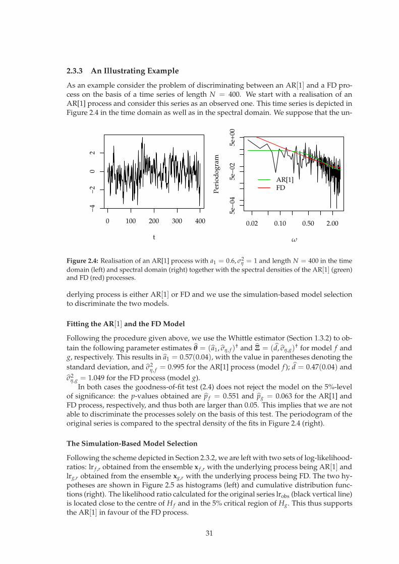
2.3.3 An Illustrating Example

As an example consider the problem of discriminating between an AR[1] and a FD pro-cess on the basis of a time series of length N = 400. We start with a realisation of anAR[1] process and consider this series as an observed one. This time series is depicted inFigure 2.4 in the time domain as well as in the spectral domain. We suppose that the un-

0 100 200 300 400

−4

−2

02

t

months

0.02 0.10 0.50 2.005e

−04

5e−

025e

+00

Per

iod

og

ram

AR[1]FD

ω

Figure 2.4: Realisation of an AR[1] process with a1 = 0.6, σ2η = 1 and length N = 400 in the time

domain (left) and spectral domain (right) together with the spectral densities of the AR[1] (green)and FD (red) processes.

derlying process is either AR[1] or FD and we use the simulation-based model selectionto discriminate the two models.

Fitting the AR[1] and the FD Model

Following the procedure given above, we use the Whittle estimator (Section 1.3.2) to ob-

tain the following parameter estimates θ = (a1, ση, f )† and Ξ = (d, ση,g)† for model f and

g, respectively. This results in a1 = 0.57(0.04), with the value in parentheses denoting the

standard deviation, and σ2η, f = 0.995 for the AR[1] process (model f ); d = 0.47(0.04) and

σ2η,g = 1.049 for the FD process (model g).

In both cases the goodness-of-fit test (2.4) does not reject the model on the 5%-levelof significance: the p-values obtained are p f = 0.551 and pg = 0.063 for the AR[1] andFD process, respectively, and thus both are larger than 0.05. This implies that we are notable to discriminate the processes solely on the basis of this test. The periodogram of theoriginal series is compared to the spectral density of the fits in Figure 2.4 (right).

The Simulation-Based Model Selection

Following the scheme depicted in Section 2.3.2, we are left with two sets of log-likelihood-ratios: lr f ,r obtained from the ensemble x f ,r with the underlying process being AR[1] andlrg,r obtained from the ensemble xg,r with the underlying process being FD. The two hy-potheses are shown in Figure 2.5 as histograms (left) and cumulative distribution func-tions (right). The likelihood ratio calculated for the original series lrobs (black vertical line)is located close to the centre of H f and in the 5% critical region of Hg. This thus supportsthe AR[1] in favour of the FD process.

31

lr

−40 −20 0 10 20

020

060

0

ω

−40 −20 0 20

0.0

0.4

0.8

lr

EC

DF

Figure 2.5: Distributions of the log-likelihood-ratio for the AR[1] (lr f , green) and the FD (lrg, red)model as histogram (left) and cumulative distributions function (right). The critical regions areindicated as filled regions and the log-likelihood-ratio for the original series is shown as blackvertical line. The distributions are obtained from R = 10 000 runs.

The visualisation of the hypotheses in Figure 2.5 provides us with an idea to what ex-tent the two models are distinguishable and which hypothesis to reject. In this examplethe distributions are well separated and the observed value is close to the centre of theAR-hypothesis but at the edge of the distribution resulting from the FD model. Addi-tional to this visual impression, we estimate also critical regions, the power of the testsand p-values in the way described above.

Estimating Critical Regions Consider the AR[1] model as the hypothesis under testand the FD as the alternative. For the given example using (2.10) we find a critical value

at α = 0.05 of lrcrit

f ,0.05 = lr f ,([500]) = 5.393. The critical region extends towards smallervalues and thus the observed value lrobs = 10.463 lies outside. Thus the hypothesis H f

“the realisation stems from an AR[1] model”, cannot be rejected

For the inverse situation of testing FD against the alternative AR[1], we find a lower

limit of a critical region at lrcrit

g,0.05 = lrg,([500]) = 1.115. The observed value is thus insideand we can reject the hypothesis that the realisation stems from an FD model.

Estimating the Power of the Test Considering again the AR[1] model as the hypothesisunder test, with (2.12) we obtain an estimate pow f (α = 0.05, g) = 0.9978. Simultaneously,

we have obtained an estimate β = 1 − pow f (α = 0.05, g) = 0.0022. This estimate of the

power being close to one is a result of the distributions being well separated. This highpower implies that H f (AR[1]) is very likely rejected for realisations from an FD process(Hg).

The corresponding power estimate for the inverse situation amounts to powg(α =

0.05, f ) = 0.999.

Estimating p-Values For the AR[1] model we estimate a p-value p f = 0.3533 using (2.11).We thus have no evidence to reject this hypothesis. Since in our example, no lrg,r exceeds

32

the observed likelihood ratio, we find pg = 0 and thus strong evidence against the FDhypothesis.

On the basis of the above procedure we can thus very confidently reject the hypothesisof the data being generated from an FD model in favour of the autoregressive alternative.In the given example, we know the underlying process and find that it was correctlyidentified.

In order to investigate whether the simulation-based model selection strategy can bereferred to as a statistical test, we have to evaluate whether the rate of rejection corre-sponds to the nominal level α.

2.3.4 Testing the Test

In the setting presented above, we straightforwardly estimated critical regions, p-valuesand the power, for testing simple hypotheses, i.e. we assume that the null as well as thealternative hypotheses are models with known parameters, namely the ML estimates forthe specified models. This is different from the situation where the parameters are notknown or, in other words, from testing composite hypotheses, i.e. the record is eithercompatible with an AR[1] or with an FD process. In the latter situation the parametersare not known but have to be estimated. This is the question we actually have to ad-dress. Thus we test the size of such a test in a simulation study. In the current setting,this implies to investigate whether the rejection rate according to the estimated p-valuescorrespond to the nominal rate α. We furthermore investigate to what extend the estimateof the power is a useful approximation.

Testing the Size

We use again the AR[1] example process and perform an extensive simulation study us-ing different values for the parameter a1 ∈ 0.1, 0.3, 0.5, 0.7, 0.9 and various sample sizesN ∈ 100, 200, 400, 800, 2 000, 4 0002 . For a1 and N fixed, we generate M = 1 000 realisa-tions. For each such realisation we use the simulation-based model selection (again with1 000 runs) to estimate p-values for a test against a FD model. The fractional differenceparameter d of this alternative hypothesis is estimated from the realisations. On the basisof this p-value for a given realisation, we can either reject or accept the null hypothesison a prescribed nominal level of significance α. The fraction of the number of rejectionsof the total number of realisations M is called the rejection rate rα. For a statistical testthis rate must agree with the nominal level α for large M, or, equivalently, rα/α → 1 forM → ∞.

Figure 2.6 shows the relative rate of rejection rα/α for three nominal levels of α. In thefour upper panels (a-d) the dependence on the sample size N is given for four values ofa1. The two bottom panels (e,f) depict the dependence on the parameter a1 for a smalland a large sample size. The largest deviations from unity in all panels can be observedfor a nominal level of α = 0.01. For this level, we expect only ten of the 1 000 realisationsto be rejected. Thus a deviation of 50% implies five instead of ten rejected realisation. Inthis range the statistic is very limited.

The plot for the N-dependence with a small autoregressive parameter (a1=0.1, panela), suggests that an increasing sample size reduces the difference between nominal level

2Obtaining results for larger N, e.g., N = 8 000 could not be accomplished within one week of computa-tion time for a given a1 and M = 1 000 runs on one node of the IBM p655 Cluster equipped with IBM Power4CPUs with 1.1 GHz.

33

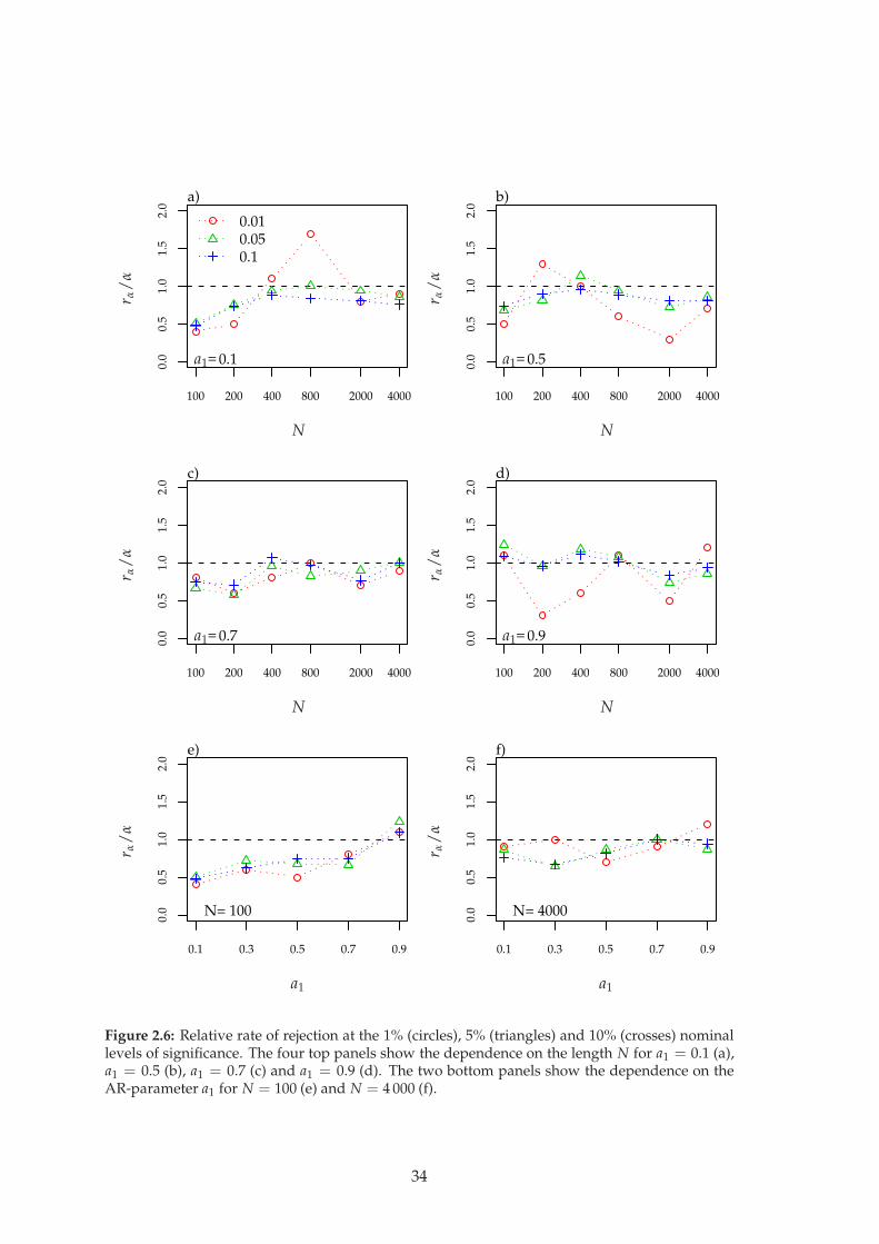
0.0

0.5

1.0

1.5

2.0

100 200 400 800 2000 4000

0.010.050.1

= 0.1

a)

ω

a1

r α/

α

N

0.0

0.5

1.0

1.5

2.0

100 200 400 800 2000 4000

= 0.5

b)

a1

r α/

αN

0.0

0.5

1.0

1.5

2.0

100 200 400 800 2000 4000

= 0.7

c)

a1

r α/

α

N

0.0

0.5

1.0

1.5

2.0

100 200 400 800 2000 4000

= 0.9

d)

a1

r α/

α

N

0.0

0.5

1.0

1.5

2.0

0.1 0.3 0.5 0.7 0.9

N= 100

e)

a1

r α/

α

0.0

0.5

1.0

1.5

2.0

0.1 0.3 0.5 0.7 0.9

N= 4000

f)

a1

r α/

α

Figure 2.6: Relative rate of rejection at the 1% (circles), 5% (triangles) and 10% (crosses) nominallevels of significance. The four top panels show the dependence on the length N for a1 = 0.1 (a),a1 = 0.5 (b), a1 = 0.7 (c) and a1 = 0.9 (d). The two bottom panels show the dependence on theAR-parameter a1 for N = 100 (e) and N = 4 000 (f).

34

and calculated rejection rate. For larger a1, the sample size does not have a clear influenceanymore (panels b-d). Except for a1 = 0.9, the rejection rates are predominantly smallerthan the corresponding nominal level. The a1-dependence for small sample size (N =100) (panel e) shows that the rejection rate increases with the autoregressive parametera1. For a1 = 0.1, we find the rejection rate being about 50% smaller than the nominallevel. Only for a1 = 0.9 more realisations of the AR[1] process are rejected than expectedfrom the value of α. For a larger sample size (N = 4 000), the mismatch between nominallevel and rejection rate reduces, especially for small a1 (panel f). In this case, we observea relative rejection rate rα/α < 1 for a1 = 0.9 and α ∈ 0.05, 0.1.

In situation where we find a rejection rate smaller than the nominal level, we speakof a conservative test; the rejection under the null hypothesis is not as likely as expected.In the opposite case of a rejection rate larger than the nominal value, one is more likelyto reject a true null hypothesis than expected. For the present example, this implies thatthe AR hypothesis is rejected in favour of an FD process. The consequence is falselydetecting LRD. Thus in the case of discriminating between an AR[1] and an FD process,special attention has to be paid to processes with large autoregressive parameters.

For the situation of the example under consideration (a1 = 0.6 and N = 400), therelative rejection rates are close to one for N = 400 and a1 = 0.5 (r0.05/0.05 = 1.14) ora1 = 0.7 (r0.05/0.05 = 0.96). We can thus expect that the selection procedure is close to astatistical test in this case.

Estimating the Power

With further simulations we study the estimates of the power for the simulation-basedmodel selection. The power is the rate of rejection for records from the alternative hy-pothesis. Thus we need to study realisations of a suitable process serving as such. In thissetting this is an FD process with a difference parameter d chosen adequately to the corre-sponding null hypothesis. This parameter changes with the length N and the parametera1 of the AR[1] process. Thus, we estimate d from 20 realisations of the null hypothesisAR[1] for given a1 and N and take the average value for the alternative hypothesis. Withthis alternative hypothesis we generate 1 000 realisations and obtain an estimate for thepower according to (2.12) for each run. This sample of power estimates is then comparedto the rate of rejection obtained from the ensemble by means of a box-plot. The results forvarious a1 and N is shown in Figure 2.7. The blue crosses mark the difference parameterused for the alternative hypothesis. The power increases with N but in a different man-ner for different a1. The most rapid increase can be observed for a1 = 0.5 and a1 = 0.7.In general the power estimates are very variable in regions of low power and especiallyfor parameters a1 = 0.1 and a1 = 0.9 where the AR[1] and the FD process have quitesimilar spectral densities. For the other two parameter values (a1 = 0.5 and a1 = 0.7)the estimate of the power is on average good. Particularly, for the setting of the examplestudied above (a1 = 0.6, N = 400), the power estimate close to one should be reliable.

In some cases, we find a fractional difference parameter d > 0.5 which correspondsto the non-stationary domain. We are, however, still able to obtain estimates and anapproximate likelihood as discussed in Section 1.3.2.

In case we cannot distinguish the two models, for example due to a low power, wecan obtain a rough estimate of the time series length needed for a satisfactorily power onthe basis of simulations, as described in the following.

35

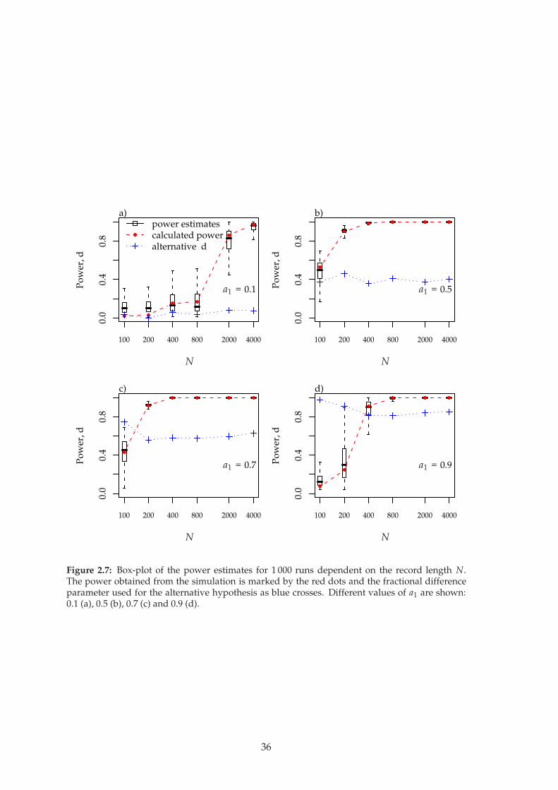
0.0

0.4

0.8

Po

wer

, d

100 200 400 800 2000 4000

= 0.1

power estimatescalculated poweralternative d

a)

ω

a1

N

0.0

0.4

0.8

Po

wer

, d

100 200 400 800 2000 4000

= 0.5

b)

a1

N

0.0

0.4

0.8

Po

wer

, d

100 200 400 800 2000 4000

= 0.7

c)

a1

N

0.0

0.4

0.8

Po

wer

, d

100 200 400 800 2000 4000

= 0.9

d)

a1

N

Figure 2.7: Box-plot of the power estimates for 1 000 runs dependent on the record length N.The power obtained from the simulation is marked by the red dots and the fractional differenceparameter used for the alternative hypothesis as blue crosses. Different values of a1 are shown:0.1 (a), 0.5 (b), 0.7 (c) and 0.9 (d).

36

2.3.5 Estimating the Required Sample Size

The power of the test changes with the length of the series under consideration. Thisis depicted in Figure 2.8. The model parameters used in the simulations are the MLestimates θ and Ξ obtained for the original time series length.

20 50 200 1000 5000

0.2

0.4

0.6

0.8

1.0

Po

wer H0: AR[1]

H0: FD

N

Figure 2.8: Power of testing the AR[1] hypothesis (green) and FD hypothesis (red) calculated forvarious lengths.

In cases where it is not possible to discriminate the models, i.e. the length of the ob-served record does not lead to satisfactory power of the test, we might repeat the pro-cedure with increasing length of the simulated series. We then get an idea what recordlength is needed to distinguish the two models. Interpretation of this result has to betreated with care, because on the one hand, we use the estimates θ and Ξ instead of the“true” parameter values. These estimates depend on the sample size N. On the otherhand, every hypothesis is trivially falsified for a sufficient length of the time series. Anincreasing power does thus not mean that we are able to decide for one model; we mightend up with rejecting both. However, for a moderate increase of sample length, we mightstill get an appropriate idea of the power.

In the context of geophysical records the lack of data basically implies to postpone theanalysis until sufficient data has been collected. In other settings, with the possibility ofinfluencing the size of the sample beforehand, this approach might be useful to designthe experiment. This ensures that a sufficient size of the sample can be taken. Then theresearch question can be answered while an unnecessary surplus of data collection canbe avoided, e.g., to reduce costs.

2.3.6 Bootstrapping the Residuals

Within the framework of FARIMA[p, d, q] models, the ensemble members x f ,r or xg,r canbe generated from a white noise process ηt using a linear filter (cf. Section 1.2.1)

xt =M

∑i=0

γiηt−i. [1.39]

In general the sum (1.39) extends over infinitively many elements M. In practical appli-cation, the filter is truncated at a suitable length. The γi can be derived from the modelparameters (??).

37

For invertible models (1.39) can be inverted to obtain the residual series rt fromthe time series xt given the model. In situations where the distribution of the residualseries is not close to a Gaussian, we might consider replacing the realisation ηt of thewhite noise process with a realisation of a bootstrap resampling of the residuals ri (??).In this way the distribution of the residuals is conserved.

2.4 Summary

We started the discussion on model selection with an example of a goodness-of-fit test: aspectral variant of the Portmanteau Test. This test is particularly suitable for the kind ofmodels used and parameter estimation strategy we pursue here. For model comparison,we suggested the standard likelihood-ratio test and the Akaike-type information criteria(AIC, BIC, HIC). These methods can be used for choosing between nested models.

Starting from a general likelihood-ratio approach, we developed a simulation-basedstrategy for the discrimination of non-nested FARIMA[p, d, q] models. The formulationof this approach is within the framework of statistical hypothesis testing, i.e. the con-cepts of critical regions, p-values, and power are used. We illustrated this method witha simulated example series from an AR[1] process. On the basis of one realisation, theAR[1] model could correctly be identified as the underlying process. The FD model asalternative hypothesis could be rejected, with a power close to one.

In order to study to what extend the estimates provided for the p-values and thepower can be interpreted in the sense of a statistical test, we performed an extensivesimulation study related to the above example. The results showed a dependence of therelative rejection rate on the parameter value a1 and on the sample size N. The quality ofthe power estimates depend as well on the sample length and on the parameter values.We find useful estimates of the power in regions of high power and especially when thespectral densities of the AR[1] and the FD process are not similar (here a1 = 0.5 anda1 = 0.7). In regions of low power and especially towards the boundaries of the interval(0, 1) for a1, estimates become highly variable and are to be interpreted with care.

If we cannot discriminate between the two models, a simulation study with an in-creased record length gives an idea how many data points are needed for a reliable de-cision. Because the simulations with increased length will be based on the parametersestimated for the observed length, the range of this analysis is limited.

Given the idea of generating ensembles from the two hypotheses under test, one canthink of other statistics than the likelihood ratio. Especially in the context of detectingLRD, statistics focusing on the low frequency behaviour might be suitable. Two statistics,one based on the log-periodogram regression and one based on the DFA are discussed inAppendix B.4. In the example presented here, the likelihood ratio as test statistic results,however, in the more powerful test.

In the following chapter, we develop a strategy to detect LRD on the basis of para-metric modelling and the model selection strategies presented and developed here.

38

Chapter 3

Detection of Long-RangeDependence

“Nothing is what it seems!”Morpheus to Neo in The Matrix, 1999

The phenomenon of long-range dependence (LRD, Section 1.1.4) has received atten-tion since the 1950s, the time the British hydrologist H. E. Hurst studied the Nile Riverminimum flows, until today (???????). Its discussion is not limited to hydrology but isprevailing in other fields of the geosciences as well as in economics (e.g., ?????). Withthis variety of applications different ways of detecting and describing the phenomenonarose. We can basically distinguish two strategies for the detection of LRD.

1. The historically older one is the search for a certain asymptotic behaviour in theautocorrelation function, in the spectrum, or similar statistics (Section 1.1.4). Theseapproaches consist of a simple parametric description of the asymptotic behaviourof the statistic under consideration in regions where these asymptotics are assumedto hold. Such strategies are referred to as semi-parametric. If the asymptotic be-haviour is sufficiently assured to hold and if the properties of the estimator areknown, as it is the case for the log-periodogram regression (Appendix. B.3.2), in-ference about LRD can be made (?). For estimators with unknown limiting dis-tributions, as, e.g., DFA-based estimation (Section 1.3.3), inference in not possiblestraightforwardly. Such approaches are referred to as heuristic; they are useful fora preliminary analysis but not for statistical inference (?).

2. An alternative strategy is a full-parametric modelling approach including modelselection as outlined in Chapter 2. The difference to semi-parametric or heuristicapproaches is that non-asymptotic behaviour is not disregarded but explicitly mod-elled. Within the likelihood framework a limiting distribution for the estimator isavailable, and thus inference about the parameter values – in particular about thefractional difference parameter d – is possible (Section 1.3). More subtle is the modelselection discussed in Chapter 2. The inference about model parameters, such as thefractional difference parameter, is only meaningful if the proper model is used. Theproblem of selecting a suitable model corresponds to selecting an adequate regionfor the log-periodogram regression (?): a small region as well as a complex modellead to a smaller bias but brings along a larger variance for the estimate, and viceversa.

39

In this chapter, we develop a strategy for the detection of LRD based on the full-parametric modelling approach and the model selection strategy proposed in Chapter 2.In the first section, we generate two example series: one from a LRD and one from aSRD process. The latter is constructed such that its realisations with a given length canbe easily mistaken for realisations of the LRD process. In the subsequent sections, theseseries are analysed with DFA and the log-periodogram regression. Finally, we developthe full-parametric strategy and illustrate its abilities to discriminate SRD and LRD withthese example series.

3.1 Constructing the Example Process

Contrary to the example studied in Section 2.3.3, we consider two processes which aresimilar in their high frequency behaviour and differ only in the low frequency region, i.e.one is LRD, the other SRD. Realisations of them are then taken as “observed” records.Based on these “observations” we aim to decide whether the underlying process is SRDor the LRD.

In order to strongly challenge the various model selection strategies, we constructa SRD process such that it mimics a given LRD process as closely as possible. To thisend, we generate a realisation of a LRD model and search for an SRD model representingthis realisation reasonably well. Within the framework of the FARIMA[p, d, q] family, asimple LRD process is the FARIMA[1, d, 0] (or, for short, FAR[1]) process. A realisationof this process can be reasonably well modelled with an ARMA[3, 2] process (for details,cf. Appendix B.5). We expect a realisation of this SRD model to be easily mistaken forstemming from the FAR[1] process. It is thus an ideal candidate to illustrate and testdetection strategies for LRD.

Figure 3.1 shows the realisation of the ARMA[3, 2] (green) and the FAR[1] process(red) in the time and frequency domain. Both realisations have N = 215 = 32 768 datapoints.

0 1000 3000 5000

−5

05

Index

Dat

a

5e−05 1e−03 5e−02

1e−

041e

+00

Po

wer

FAR[1]ARMA[3,2]

ω

Figure 3.1: Time domain (left) and frequency domain (right) representation of the ARMA[3, 2]realisation (green, a1 = 2.178, a2 = −1.488, a3 = 0.309, b1 = −1.184, b2 = 0.218) compared to theFAR[1] realisation (red, d = 0.3, a1 = 0.7).

For the analyses in the following sections, we consider these two records as “ob-served” data and try to infer the underlying processes.

40

3.2 Detrended Fluctuation Analysis

For the detection of LRD it has become a widely used practice to compare the DFA fluctu-ation function (Section 1.3.3) in a double-logarithmic plot to an expected asymptotic slopefor SRD or uncorrelated processes (e.g., ????). For the “observed” records, obtained fromthe ARMA[3, 2] and the FAR[1] process, we depict these fluctuation function in Figure 3.2.From a visual inspectation of the left panel one might be tempted to consider the slopes H

0.5 1.5 2.5 3.5

−0.

50.

51.

52.

5

log s

log

F(s

) 0.5

0.75

FAR[1]ARMA[3,2]

[1/

0.5 1.5 2.5 3.5−

0.5

0.5

1.5

2.5

log s

log

F(s

)

3.52.51.5

0.520.700.80

Hlog s ≥

Figure 3.2: DFA1 fluctuation functions in double logarithmic representation for the ARMA[3, 2](green) and the FAR[1] (red) realisation (left). The two solid black lines mark the asymptoticbehaviour expected for SRD, or uncorrelated, processes (H = 0.5) and for a LRD process withH = 0.75. The dashed vertical line marks the lower bound of scales considered. Straight linefits for various ranges of scales to the DFA1 fluctuation function of the ARMA[3, 2] realisation areshown in the right panel.

of both fluctuation functions being approximately constant with H > 0.5 for large scaless. For log s > 2, for example, the plot suggests that in both cases the slopes are rathercompatible with H = 0.75 than with H = 0.5. Thus, this provides no evidence for anSRD process in neither case. Following this line of argument, we would falsely infer aLRD process with H = 0.75 underlying both realisations. This demonstrates that a reli-able discrimination of realisations from LRD or SRD processes is not easily achieved onthe basis of DFA. Consequently such results should be interpreted with care.

A more detailed analysis of the fluctuation function of the ARMA[3, 2] realisation inthe right panel of Figure 3.2 shows already that the slope systematically increases withdecreasing lower bound of scales for the fit (i.e. an increasing range of scales considered).This should raise awareness and provides first evidence that the asymptotic behaviourhas not been reached. If it had been reached, the slope should fluctuate around a constantvalue but should not exhibit a systematic variation. A critical review on the use of DFAto infer LRD explicitely addressing this point is given in Appendix A together with adetailed analysis of bias and variance for Hurst exponent estimation.

3.3 Log-Periodogram Regression

Contrary to a DFA-based estimator, a limiting distribution does exist for the estimator dlp

based on the log-periodogram regression (Appendix B.3.2). We can thus provide confi-dence intervals and test whether the estimate for the fractional difference parameter is

41

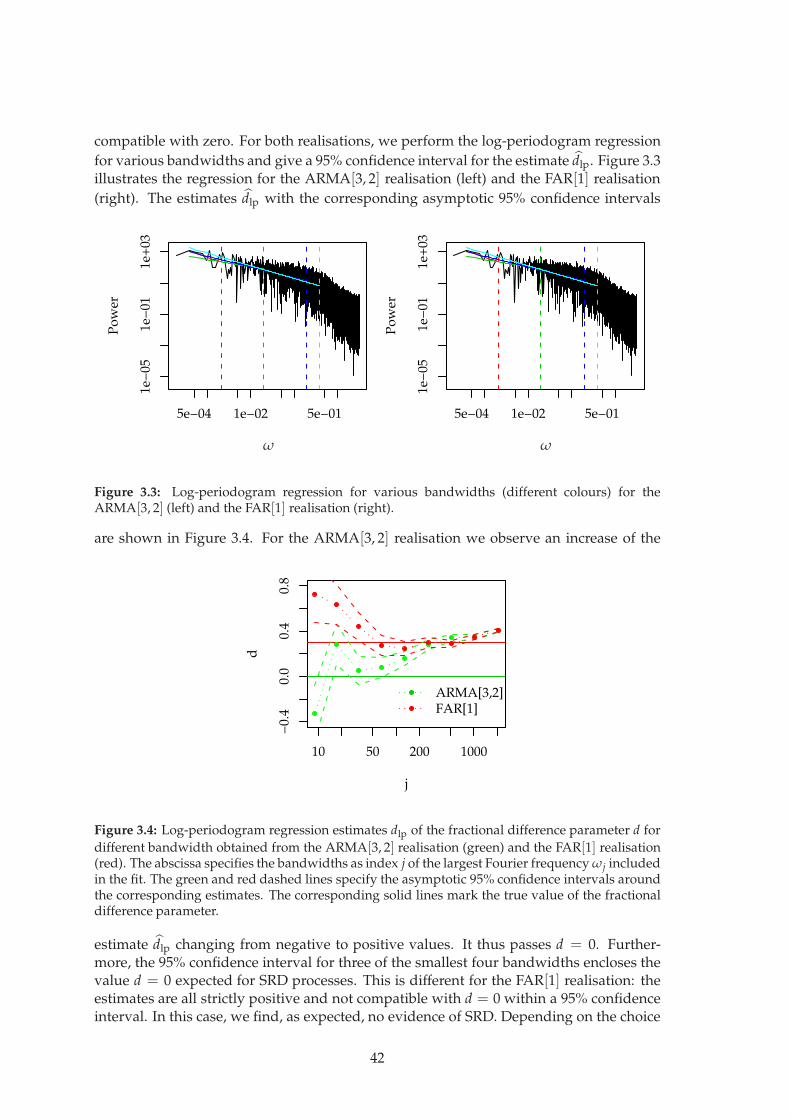
compatible with zero. For both realisations, we perform the log-periodogram regression

for various bandwidths and give a 95% confidence interval for the estimate dlp. Figure 3.3illustrates the regression for the ARMA[3, 2] realisation (left) and the FAR[1] realisation

(right). The estimates dlp with the corresponding asymptotic 95% confidence intervals

5e−04 1e−02 5e−01

1e−

051e

−01

1e+

03

Po

wer

ω

5e−04 1e−02 5e−011e

−05

1e−

011e

+03

Po

wer

ω

Figure 3.3: Log-periodogram regression for various bandwidths (different colours) for theARMA[3, 2] (left) and the FAR[1] realisation (right).

are shown in Figure 3.4. For the ARMA[3, 2] realisation we observe an increase of the

10 50 200 1000

−0.

40.

00.

40.

8

j

d

ARMA[3,2]FAR[1]

Figure 3.4: Log-periodogram regression estimates dlp of the fractional difference parameter d for

different bandwidth obtained from the ARMA[3, 2] realisation (green) and the FAR[1] realisation(red). The abscissa specifies the bandwidths as index j of the largest Fourier frequency ωj includedin the fit. The green and red dashed lines specify the asymptotic 95% confidence intervals aroundthe corresponding estimates. The corresponding solid lines mark the true value of the fractionaldifference parameter.

estimate dlp changing from negative to positive values. It thus passes d = 0. Further-more, the 95% confidence interval for three of the smallest four bandwidths encloses thevalue d = 0 expected for SRD processes. This is different for the FAR[1] realisation: theestimates are all strictly positive and not compatible with d = 0 within a 95% confidenceinterval. In this case, we find, as expected, no evidence of SRD. Depending on the choice

42

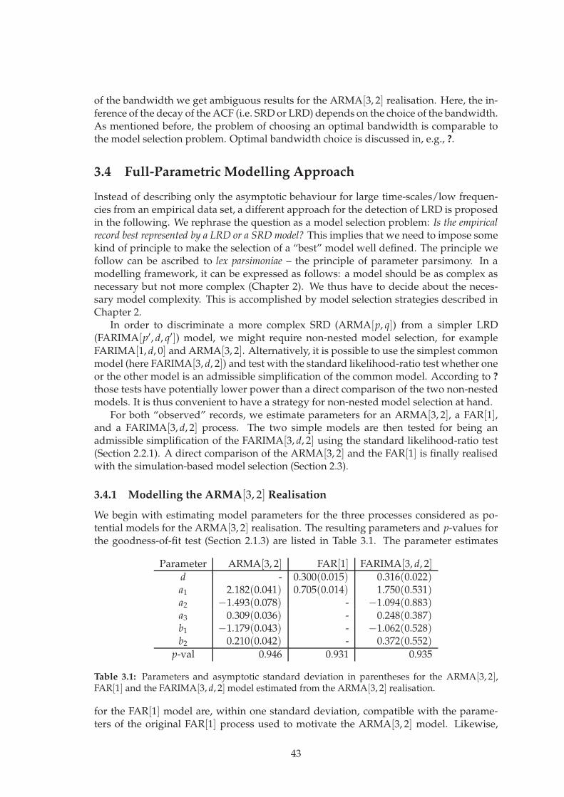
of the bandwidth we get ambiguous results for the ARMA[3, 2] realisation. Here, the in-ference of the decay of the ACF (i.e. SRD or LRD) depends on the choice of the bandwidth.As mentioned before, the problem of choosing an optimal bandwidth is comparable tothe model selection problem. Optimal bandwidth choice is discussed in, e.g., ?.

3.4 Full-Parametric Modelling Approach

Instead of describing only the asymptotic behaviour for large time-scales/low frequen-cies from an empirical data set, a different approach for the detection of LRD is proposedin the following. We rephrase the question as a model selection problem: Is the empiricalrecord best represented by a LRD or a SRD model? This implies that we need to impose somekind of principle to make the selection of a “best” model well defined. The principle wefollow can be ascribed to lex parsimoniae – the principle of parameter parsimony. In amodelling framework, it can be expressed as follows: a model should be as complex asnecessary but not more complex (Chapter 2). We thus have to decide about the neces-sary model complexity. This is accomplished by model selection strategies described inChapter 2.

In order to discriminate a more complex SRD (ARMA[p, q]) from a simpler LRD(FARIMA[p′, d, q′]) model, we might require non-nested model selection, for exampleFARIMA[1, d, 0] and ARMA[3, 2]. Alternatively, it is possible to use the simplest commonmodel (here FARIMA[3, d, 2]) and test with the standard likelihood-ratio test whether oneor the other model is an admissible simplification of the common model. According to ?

those tests have potentially lower power than a direct comparison of the two non-nestedmodels. It is thus convenient to have a strategy for non-nested model selection at hand.

For both “observed” records, we estimate parameters for an ARMA[3, 2], a FAR[1],and a FARIMA[3, d, 2] process. The two simple models are then tested for being anadmissible simplification of the FARIMA[3, d, 2] using the standard likelihood-ratio test(Section 2.2.1). A direct comparison of the ARMA[3, 2] and the FAR[1] is finally realisedwith the simulation-based model selection (Section 2.3).

3.4.1 Modelling the ARMA[3, 2] Realisation

We begin with estimating model parameters for the three processes considered as po-tential models for the ARMA[3, 2] realisation. The resulting parameters and p-values forthe goodness-of-fit test (Section 2.1.3) are listed in Table 3.1. The parameter estimates

Parameter ARMA[3, 2] FAR[1] FARIMA[3, d, 2]d - 0.300(0.015) 0.316(0.022)a1 2.182(0.041) 0.705(0.014) 1.750(0.531)a2 −1.493(0.078) - −1.094(0.883)a3 0.309(0.036) - 0.248(0.387)b1 −1.179(0.043) - −1.062(0.528)b2 0.210(0.042) - 0.372(0.552)

p-val 0.946 0.931 0.935

Table 3.1: Parameters and asymptotic standard deviation in parentheses for the ARMA[3, 2],FAR[1] and the FARIMA[3, d, 2] model estimated from the ARMA[3, 2] realisation.

for the FAR[1] model are, within one standard deviation, compatible with the parame-ters of the original FAR[1] process used to motivate the ARMA[3, 2] model. Likewise,

43

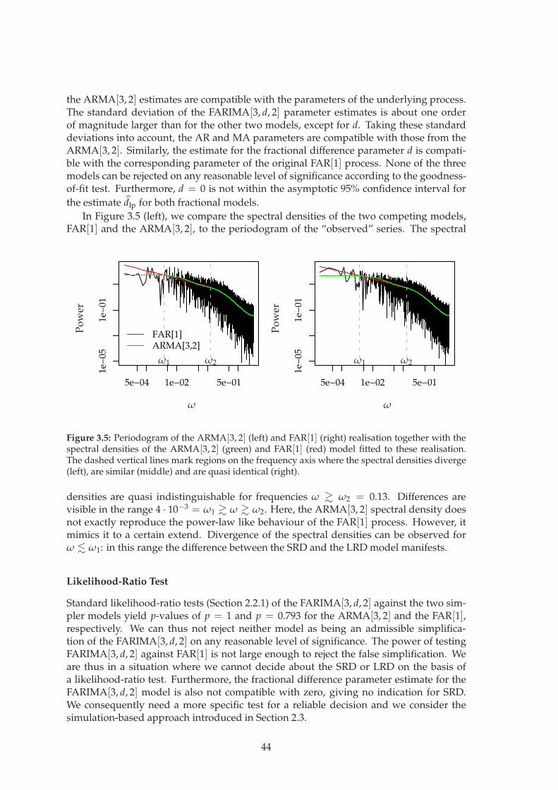
the ARMA[3, 2] estimates are compatible with the parameters of the underlying process.The standard deviation of the FARIMA[3, d, 2] parameter estimates is about one orderof magnitude larger than for the other two models, except for d. Taking these standarddeviations into account, the AR and MA parameters are compatible with those from theARMA[3, 2]. Similarly, the estimate for the fractional difference parameter d is compati-ble with the corresponding parameter of the original FAR[1] process. None of the threemodels can be rejected on any reasonable level of significance according to the goodness-of-fit test. Furthermore, d = 0 is not within the asymptotic 95% confidence interval for

the estimate dlp for both fractional models.

In Figure 3.5 (left), we compare the spectral densities of the two competing models,FAR[1] and the ARMA[3, 2], to the periodogram of the “observed” series. The spectral

5e−04 1e−02 5e−01

1e−

051e

−01

FAR[1]ARMA[3,2]

ω

Po

wer

ω1 ω2

5e−04 1e−02 5e−01

1e−

051e

−01

ω

Po

wer

ω1 ω2

Figure 3.5: Periodogram of the ARMA[3, 2] (left) and FAR[1] (right) realisation together with thespectral densities of the ARMA[3, 2] (green) and FAR[1] (red) model fitted to these realisation.The dashed vertical lines mark regions on the frequency axis where the spectral densities diverge(left), are similar (middle) and are quasi identical (right).

densities are quasi indistinguishable for frequencies ω & ω2 = 0.13. Differences arevisible in the range 4 · 10−3 = ω1 & ω & ω2. Here, the ARMA[3, 2] spectral density doesnot exactly reproduce the power-law like behaviour of the FAR[1] process. However, itmimics it to a certain extend. Divergence of the spectral densities can be observed forω . ω1: in this range the difference between the SRD and the LRD model manifests.

Likelihood-Ratio Test

Standard likelihood-ratio tests (Section 2.2.1) of the FARIMA[3, d, 2] against the two sim-pler models yield p-values of p = 1 and p = 0.793 for the ARMA[3, 2] and the FAR[1],respectively. We can thus not reject neither model as being an admissible simplifica-tion of the FARIMA[3, d, 2] on any reasonable level of significance. The power of testingFARIMA[3, d, 2] against FAR[1] is not large enough to reject the false simplification. Weare thus in a situation where we cannot decide about the SRD or LRD on the basis ofa likelihood-ratio test. Furthermore, the fractional difference parameter estimate for theFARIMA[3, d, 2] model is also not compatible with zero, giving no indication for SRD.We consequently need a more specific test for a reliable decision and we consider thesimulation-based approach introduced in Section 2.3.

44

Simulation-Based Model Selection

Analogously to the procedure outlined in Section 2.3.2, we now perform the simulation-based model selection with the likelihood ratio as test statistic. The two models we con-sider as candidates for the underlying process are the FAR[1] and the ARMA[3, 2]. Tofacilitate the presentation, we denote in the following the ARMA[3, 2] and FAR[1] pro-cess as model f and g, respectively.

Figure 3.6 shows the cumulative distribution functions of the two log-likelihood-ratios. We find the value obtained for the “observed” record lrobs well outside the critical

−20 −10 0 10 20

0.0

0.2

0.4

0.6

0.8

1.0

lr

EC

DF

FAR[1]ARMA[3,2]Observed

Figure 3.6: Empirical cumulative distribution function of log-likelihood-ratios lr f ,r (green) andlrg,r (red) obtained from 1 100 simulations. The critical regions upto α-levels of 0.05 are filled withthe respective color. The log-likelihood-ratio lrobs for the observed series is shown as a verticalline.

region of model f and inside the critical region of model g. The estimate of the power oftesting H f against Hg for the specified critical level α = 0.05 yields pow f (0.05, g) = 0.979.

For the inverse situation of testing Hg against H f we find powg(0.05, f ) = 0.977. We can

thus very confidently reject Hg (FAR[1]) in favour of H f (ARMA[3, 2]) and correctly iden-tify the underlying process.

3.4.2 Modelling the FAR[1] Realisation

Next, we estimate the model parameters obtained from the FAR[1] realisation. The re-sulting paramters and p-values for the goodness-of-fit test (Section 2.1.3) are listed inTable 3.2. Again, no model can be rejected on the basis of the goodness-of-fit test andthe original FAR[1] parameters are recovered within one standard deviation. Also for theFARMA[3, d, 2] model, the estimates are compatible with the parameters of the originalFAR[1] process.

Figure 3.5 (right) compares the ARMA[3, 2] and the FAR[1] spectral densities to theperiodogram of the FAR[1] realisation. The picture is very similar to the left panel in the

45

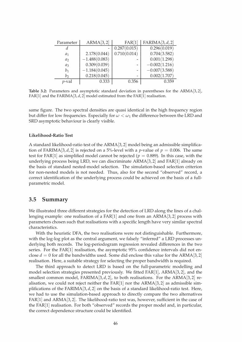
Parameter ARMA[3, 2] FAR[1] FARIMA[3, d, 2]d - 0.287(0.015) 0.296(0.019)a1 2.178(0.044) 0.710(0.014) 0.704(3.582)a2 −1.488(0.083) - 0.001(1.298)a3 0.309(0.039) - −0.002(1.216)b1 −1.184(0.045) - −0.007(3.588)b2 0.218(0.045) - 0.002(1.707)

p-val 0.333 0.356 0.359

Table 3.2: Parameters and asymptotic standard deviation in parentheses for the ARMA[3, 2],FAR[1] and the FARIMA[3, d, 2] model estimated from the FAR[1] realisation.

same figure. The two spectral densities are quasi identical in the high frequency regionbut differ for low frequencies. Especially for ω < ω1 the difference between the LRD andSRD asymptotic behaviour is clearly visible.

Likelihood-Ratio Test

A standard likelihood-ratio test of the ARMA[3, 2] model being an admissible simplifica-tion of FARIMA[3, d, 2] is rejected on a 5%-level with a p-value of p = 0.006. The sametest for FAR[1] as simplified model cannot be rejected (p = 0.889). In this case, with theunderlying process being LRD, we can discriminate ARMA[3, 2] and FAR[1] already onthe basis of standard nested-model selection. The simulation-based selection criterionfor non-nested models is not needed. Thus, also for the second “observed” record, acorrect identification of the underlying process could be achieved on the basis of a full-parametric model.

3.5 Summary

We illustrated three different strategies for the detection of LRD along the lines of a chal-lenging example: one realisation of a FAR[1] and one from an ARMA[3, 2] process withparameters chosen such that realisations with a specific length have very similar spectralcharacteristics.

With the heuristic DFA, the two realisations were not distinguishable. Furthermore,with the log-log plot as the central argument, we falsely “inferred” a LRD processes un-derlying both records. The log-periodogram regression revealed differences in the twoseries. For the FAR[1] realisation, the asymptotic 95% confidence intervals did not en-close d = 0 for all the bandwidths used. Some did enclose this value for the ARMA[3, 2]realisation. Here, a suitable strategy for selecting the proper bandwidth is required.

The third approach to detect LRD is based on the full-parametric modelling andmodel selection strategies presented previously. We fitted FAR[1], ARMA[3, 2], and thesmallest common model, FARIMA[3, d, 2], to both realisations. For the ARMA[3, 2] re-alisation, we could not reject neither the FAR[1] nor the ARMA[3, 2] as admissible sim-plifications of the FARIMA[3, d, 2] on the basis of a standard likelihood-ratio test. Here,we had to use the simulation-based approach to directly compare the two alternativesFAR[1] and ARMA[3, 2]. The likelihood-ratio test was, however, sufficient in the case ofthe FAR[1] realisation. For both “observed” records the proper model and, in particular,the correct dependence structure could be identified.

46

This example illustrated the reliability of the full-parametric modelling approach withrespect to the detection of LRD. Furthermore, it turned out that the standard model se-lection, in some cases, such as the example at hand, does not have enough power to dis-criminate the two alternatives under consideration. In such cases, a suitable strategy forthe discrimination of non-nested models, such as the simulation-based model selection,is required

The approach presented here, i.e. rephrasing the problem of detecting LRD as a modelselection problem, is different from other approaches mainly because of the direct com-parison of the most suitable SRD and the most suitable LRD process. A pivotal element inthis model comparison is the model selection strategy based on the log-likelihood-ratio.

47

48

Appendices

49

Appendix A

Review of Detrended FluctuationAnalysis

Detrended fluctuation analysis (DFA, Section 1.3.3) has been widely used to infer a LRDprocess from empirical time series and also to quantify the strength of the dependence,i.e. estimating the Hurst exponent H, or, equivalently, the fractional difference parameterd = H − 0.5 (e.g. ????). Little work has been done on characterising the inferential powerof DFA and the properties of the estimator for the Hurst exponent, e.g., quantifying biasand variance. In this chapter, we present a simulation study which provides estimatesof bias and variance for power-law noise processes. Furthermore, we critically reviewthe limits of the method to infer LRD, suggest refinements and point to typical pitfalls.Finally, we exemplify the discussion with an analysis of the Prague daily temperatureanomalies.

A.1 Bias and Variance for Self-Similar Increment Processes

Analogously to the work of ? and ?, we use Monte Carlo (MC) simulations to study thebias and variance of the estimator HDFAn for DFA1 and DFA2 (n = 1, 2) introduced inSection 1.3.3. In addition to a white noise process, we consider a process with a spectraldensity S(ω) = |ω|−β, also referred to as power-law noise. The spectral density of thisprocess is similar to the one of fGn or FD processes; especially the asymptotic behaviourfor low frequencies ω is the same. Realisations of power-law noise with a prescribedexponent β = 2H − 1 can be obtained using the inverse Fourier transform (Section 1.4; ?).

Bias

We estimate the bias and variance from MC ensembles of realisations from power-lawnoise with different length N and prescribed Hurst exponents 0 < H < 1. The estimateHDFAn is obtained as the slope of a straight line fit to log F(s) versus log s for s > 10. Wecalculate the bias using

bias(HDFAn) = HDFAn − H, (A.1)

with the bar denoting the ensemble mean. For HDFA1 and HDFA2 and an ensemble size of2 500 runs the bias is shown in Figure A.1. The estimator based on DFA1 exhibits a posi-tive bias for power-law noise with 0 < H < 0.5, increasing with decreasing H. The biasreduces with an increasing record length. This is in line with an analytical result derivedby ?. In contrast, we find a negative bias for 0.5 < H < 1, increasing in magnitude with

51

0.0 0.2 0.4 0.6 0.8 1.0

−0.

20.

00.

10.

2

DFA1H

Bia

sα

0.0 0.2 0.4 0.6 0.8 1.0

−0.

20.

00.

10.

2

DFA1H

Bia

sFigure A.1: Bias of HDFA1 (left) and HDFA2 (right). The bias is estimated from a MC ensemble ofpower-law noise realisations with a prescribed Hurst exponent H and various sample lengths N.

H. An increasing record length reduces the bias faster than for 0 < H < 0.5. For thewhite noise process (H = 0.5) no bias is observed for all length of the records. This “neu-tral point” moves towards H ≈ 0.6 for the DFA2 based estimator. This is accompaniedwith an overall increase of the bias.

Variance

The variance of HDFAn estimated from the same ensemble is shown in Figure A.2. A strik-ing difference to the previous plot is the asymmetry. The variance var(HDFA1) increasesmonotonically with 0 < H < 1. This implies that for a given length N the Hurst exponentcan be estimated more precisely for 0 < H < 0.5 then for a white noise process (H = 0.5).Furthermore, Figure A.2 depicts a decreases in variance with the length N of the series.

0.0 0.2 0.4 0.6 0.8 1.0

0.00

00.

004

0.00

8

DFA1H

Var

ian

ce

0.0 0.2 0.4 0.6 0.8 1.0

0.00

00.

004

0.00

8

DFA2H

Var

ian

ce

Figure A.2: Variance of HDFA1 (left) and HDFA2 (right). The variance is estimated from a MCensemble of power-law noise realisations with a prescribed Hurst exponent H. The colour codingof the record length is analogue to Fig. A.1.

Figures A.1 and A.2 allow for a quick and rough estimate of bias and variance for

52

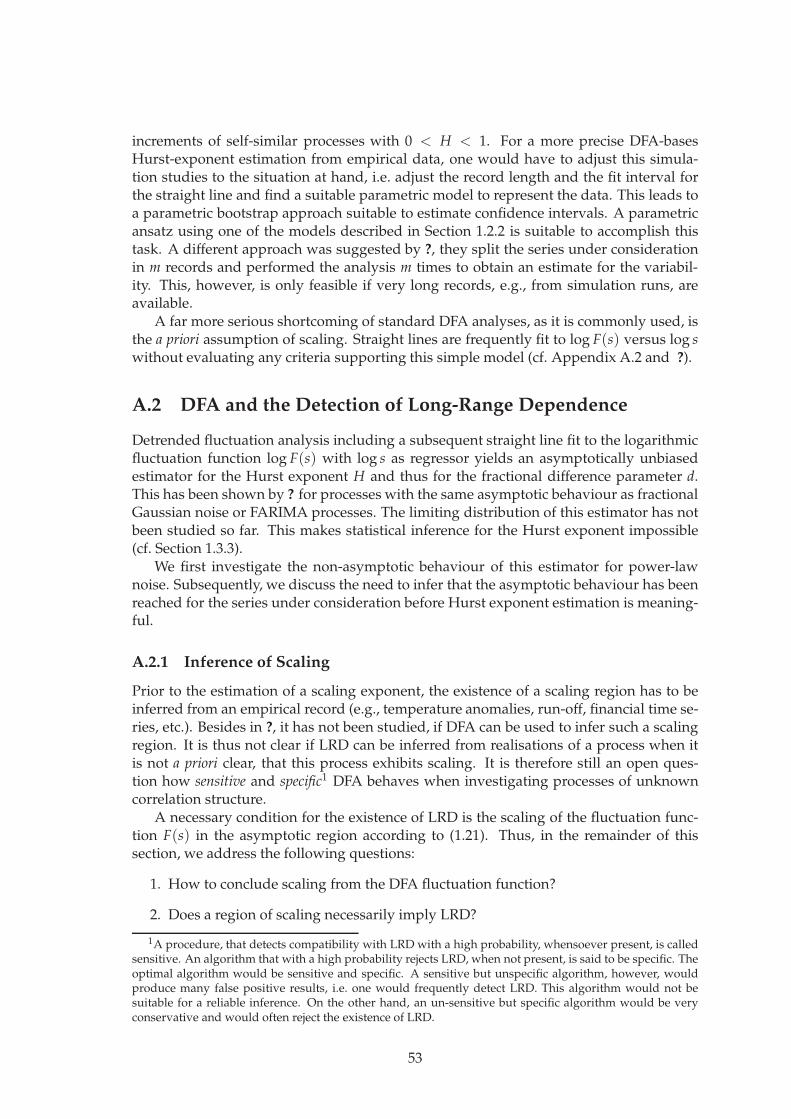
increments of self-similar processes with 0 < H < 1. For a more precise DFA-basesHurst-exponent estimation from empirical data, one would have to adjust this simula-tion studies to the situation at hand, i.e. adjust the record length and the fit interval forthe straight line and find a suitable parametric model to represent the data. This leads toa parametric bootstrap approach suitable to estimate confidence intervals. A parametricansatz using one of the models described in Section 1.2.2 is suitable to accomplish thistask. A different approach was suggested by ?, they split the series under considerationin m records and performed the analysis m times to obtain an estimate for the variabil-ity. This, however, is only feasible if very long records, e.g., from simulation runs, areavailable.

A far more serious shortcoming of standard DFA analyses, as it is commonly used, isthe a priori assumption of scaling. Straight lines are frequently fit to log F(s) versus log swithout evaluating any criteria supporting this simple model (cf. Appendix A.2 and ?).

A.2 DFA and the Detection of Long-Range Dependence

Detrended fluctuation analysis including a subsequent straight line fit to the logarithmicfluctuation function log F(s) with log s as regressor yields an asymptotically unbiasedestimator for the Hurst exponent H and thus for the fractional difference parameter d.This has been shown by ? for processes with the same asymptotic behaviour as fractionalGaussian noise or FARIMA processes. The limiting distribution of this estimator has notbeen studied so far. This makes statistical inference for the Hurst exponent impossible(cf. Section 1.3.3).

We first investigate the non-asymptotic behaviour of this estimator for power-lawnoise. Subsequently, we discuss the need to infer that the asymptotic behaviour has beenreached for the series under consideration before Hurst exponent estimation is meaning-ful.

A.2.1 Inference of Scaling

Prior to the estimation of a scaling exponent, the existence of a scaling region has to beinferred from an empirical record (e.g., temperature anomalies, run-off, financial time se-ries, etc.). Besides in ?, it has not been studied, if DFA can be used to infer such a scalingregion. It is thus not clear if LRD can be inferred from realisations of a process when itis not a priori clear, that this process exhibits scaling. It is therefore still an open ques-tion how sensitive and specific1 DFA behaves when investigating processes of unknowncorrelation structure.

A necessary condition for the existence of LRD is the scaling of the fluctuation func-tion F(s) in the asymptotic region according to (1.21). Thus, in the remainder of thissection, we address the following questions:

1. How to conclude scaling from the DFA fluctuation function?

2. Does a region of scaling necessarily imply LRD?

1A procedure, that detects compatibility with LRD with a high probability, whensoever present, is calledsensitive. An algorithm that with a high probability rejects LRD, when not present, is said to be specific. Theoptimal algorithm would be sensitive and specific. A sensitive but unspecific algorithm, however, wouldproduce many false positive results, i.e. one would frequently detect LRD. This algorithm would not besuitable for a reliable inference. On the other hand, an un-sensitive but specific algorithm would be veryconservative and would often reject the existence of LRD.

53

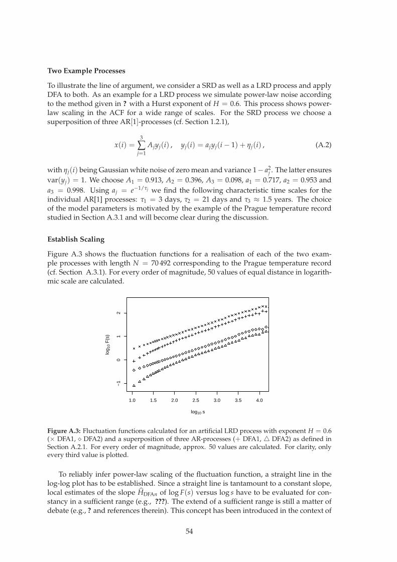
Two Example Processes

To illustrate the line of argument, we consider a SRD as well as a LRD process and applyDFA to both. As an example for a LRD process we simulate power-law noise accordingto the method given in ? with a Hurst exponent of H = 0.6. This process shows power-law scaling in the ACF for a wide range of scales. For the SRD process we choose asuperposition of three AR[1]-processes (cf. Section 1.2.1),

x(i) =3

∑j=1

Ajyj(i) , yj(i) = ajyj(i − 1) + ηj(i) , (A.2)

with ηj(i) being Gaussian white noise of zero mean and variance 1− a2j . The latter ensures

var(yj) = 1. We choose A1 = 0.913, A2 = 0.396, A3 = 0.098, a1 = 0.717, a2 = 0.953 and

a3 = 0.998. Using aj = e−1/τj we find the following characteristic time scales for theindividual AR[1] processes: τ1 = 3 days, τ2 = 21 days and τ3 ≈ 1.5 years. The choiceof the model parameters is motivated by the example of the Prague temperature recordstudied in Section A.3.1 and will become clear during the discussion.

Establish Scaling

Figure A.3 shows the fluctuation functions for a realisation of each of the two exam-ple processes with length N = 70 492 corresponding to the Prague temperature record(cf. Section A.3.1). For every order of magnitude, 50 values of equal distance in logarith-mic scale are calculated.

1.0 1.5 2.0 2.5 3.0 3.5 4.0

−1

01

2

log10 s

log 1

0 F

(s)

Figure A.3: Fluctuation functions calculated for an artificial LRD process with exponent H = 0.6(× DFA1, ⋄ DFA2) and a superposition of three AR-processes (+ DFA1, DFA2) as defined inSection A.2.1. For every order of magnitude, approx. 50 values are calculated. For clarity, onlyevery third value is plotted.

To reliably infer power-law scaling of the fluctuation function, a straight line in thelog-log plot has to be established. Since a straight line is tantamount to a constant slope,local estimates of the slope HDFAn of log F(s) versus log s have to be evaluated for con-stancy in a sufficient range (e.g., ???). The extend of a sufficient range is still a matter ofdebate (e.g., ? and references therein). This concept has been introduced in the context of

54

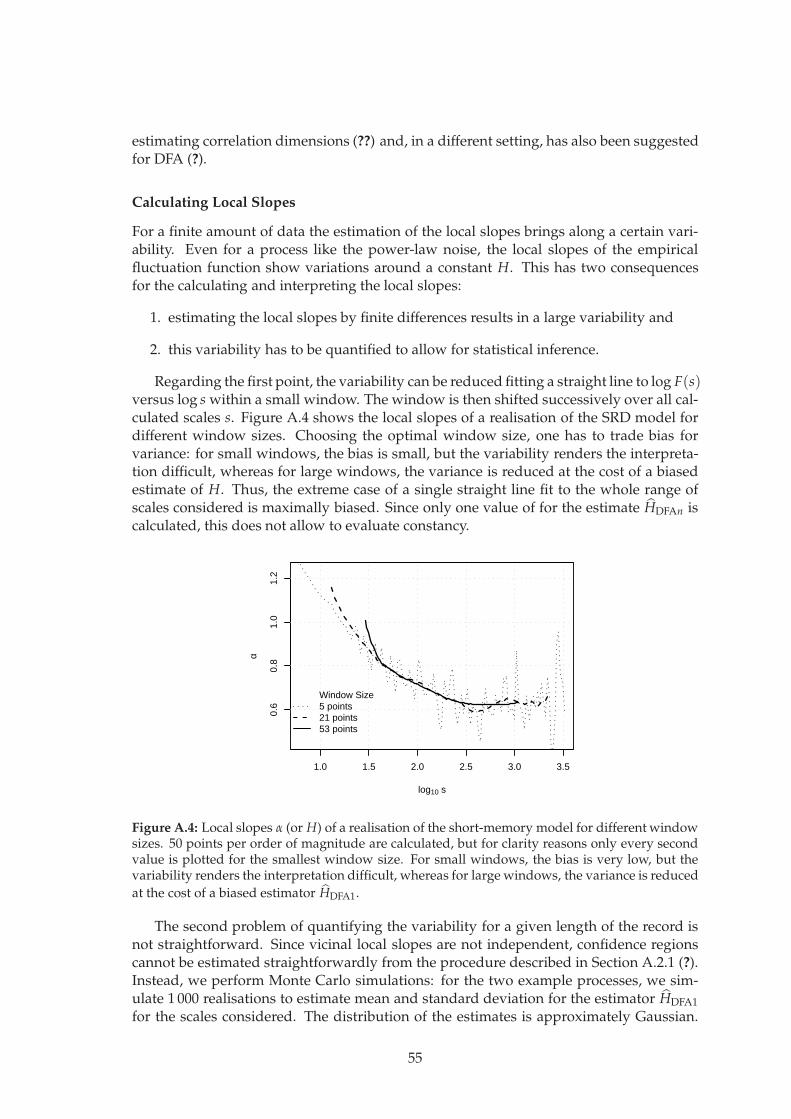
estimating correlation dimensions (??) and, in a different setting, has also been suggestedfor DFA (?).

Calculating Local Slopes

For a finite amount of data the estimation of the local slopes brings along a certain vari-ability. Even for a process like the power-law noise, the local slopes of the empiricalfluctuation function show variations around a constant H. This has two consequencesfor the calculating and interpreting the local slopes:

1. estimating the local slopes by finite differences results in a large variability and

2. this variability has to be quantified to allow for statistical inference.

Regarding the first point, the variability can be reduced fitting a straight line to log F(s)versus log s within a small window. The window is then shifted successively over all cal-culated scales s. Figure A.4 shows the local slopes of a realisation of the SRD model fordifferent window sizes. Choosing the optimal window size, one has to trade bias forvariance: for small windows, the bias is small, but the variability renders the interpreta-tion difficult, whereas for large windows, the variance is reduced at the cost of a biasedestimate of H. Thus, the extreme case of a single straight line fit to the whole range ofscales considered is maximally biased. Since only one value of for the estimate HDFAn iscalculated, this does not allow to evaluate constancy.

1.0 1.5 2.0 2.5 3.0 3.5

0.6

0.8

1.0

1.2

log10 s

α

Window Size5 points21 points53 points

Figure A.4: Local slopes α (or H) of a realisation of the short-memory model for different windowsizes. 50 points per order of magnitude are calculated, but for clarity reasons only every secondvalue is plotted for the smallest window size. For small windows, the bias is very low, but thevariability renders the interpretation difficult, whereas for large windows, the variance is reduced

at the cost of a biased estimator HDFA1.

The second problem of quantifying the variability for a given length of the record isnot straightforward. Since vicinal local slopes are not independent, confidence regionscannot be estimated straightforwardly from the procedure described in Section A.2.1 (?).Instead, we perform Monte Carlo simulations: for the two example processes, we sim-ulate 1 000 realisations to estimate mean and standard deviation for the estimator HDFA1

for the scales considered. The distribution of the estimates is approximately Gaussian.

55

Thus, we employ the interval [HDFA1 − 1.96σ, HDFA1 + 1.96σ] as estimates of the 95% con-fidence region, with the bar denoting again the ensemble mean. σ2 is the variance ofHDFA1 estimated from the ensemble.

Inferring Scaling for the Example Records

Figure A.5 displays the local slopes of the DFA1 (a) and DFA2 (b) fluctuation functions,estimated from one realisation of each of the example models. The realisation of the LRD

1.5 2.0 2.5 3.0 3.5 4.0

0.4

0.6

0.8

1.0

1.2

1.4

log10 s

α

(a)

months]

1.5 2.0 2.5 3.0 3.5 4.0

0.4

0.6

0.8

1.0

1.2

1.4

log10 s

α

(b)

Figure A.5: Local slopes α (or H) of the DFA1 (a) and DFA2 (b) fluctuation function calculated foran artificial LRD process with exponent H = 0.6 (×) and a superposition of three AR-processes(+) as defined in Section A.2.1 (window size 21 points). The dashed and the dotted lines borderthe shadowed 1.96σ intervals obtained from 1 000 realisations of the two processes, respectively.

process shows fluctuations around a constant H within the corresponding 1.96σ interval,increasing like σ ∝

√s (?). The local slope HDFA1(s) of the SRD realisation, however,

decreases constantly in the beginning and basically follows the local slope of the LRD re-alisation for scales larger than log s ≈ 2.5. Thus, for a certain choice of parameters, a SRDmodel can mimic scaling in a finite range. Due to the principle of variance superpositionfor DFA (?) a suitable superposition of three AR[1] processes produces this effect in thefluctuation function analogously to the same effect in the spectral domain described in ?.

Investigating for LRD one studies primarily the behaviour on large scales s or smallfrequencies assuming that influences from low frequencies are negligible here and do notbias the estimation of the LRD parameter. In our example, the 1.96σ-cones from the LRDand SRD process are virtually indistinguishable in this range. Thus, based on the givenrecord length and only considering large s, one cannot distinguish the realisations of thetwo models by means of DFA. For longer time series, the cones would shrink and theregion of overlapping would become smaller.

Inference of SRD

However, a general dilemma related to the inference of LRD emerges: For a finite timeseries, one will always find a SRD model to describe the data (?). Thus, considering theinference of LRD, DFA is sensitive, but not specific. An alternative ansatz is to investigateif the underlying process is SRD. This requires

1. to show compatibility with a SRD model and

2. to exclude possible LRD models.

56

The first condition is always fulfilled, since one will always find a SRD model to describea finite data set. The second condition is not fulfilled for the given example, because therecord length is not sufficient to detect the SRD character H = 0.5 for large s of the AR-model by means of DFA. For longer time series as shown in Figure A.6, when a plateauof H = 0.5 is identifiable, LRD can be excluded and the specificity of DFA to infer SRDincreases.

A.2.2 Pitfalls

We discuss typical difficulties for DFA and similar heuristic approaches. Problems arisefor example when investigating the results only in a double logarithmic plot, or, if theobserved behaviour is not consistent with the asymptotic behaviour. Also the transferfrom a scaling exponent of the fluctuation function to the ACF is only possible in theasymptotic limit.

The Double Logarithmic Plot

Investigating only the double logarithmic plot of the fluctuation function, one is temptedto rashly conclude for LRD. Due to properties of the logarithm, fluctuations are sup-pressed in a double logarithmic plot and the deviation from a straight line is not easilyvisible (?). Also, restricting the analysis to a straight line in the log-log plot forces F(s)in the procrustean bed of power-laws. It will always yield some value for the slope butthe suitability of the linear description is not evaluated. For the inference of LRD, thisprocedure would be sensitive but not specific. This results in attributing LRD to all pro-cesses with an estimate HDFAn > 0.5 for the largest scales observed. Such a result wouldtrivialise the concept of LRD and provide no insight into the process. Thus, to reliablyinfer a power-law, a straight line may not be assumed a priori but has to be established, asdiscussed in Section A.2.1. Even if scaling is present, it is difficult to determine the begin-ning and ending of the scaling region in the log-log plot. However, the estimate HDFAn

derived from a straight line fit strongly depends on the fit boundaries if the realisationdoes not stem from a scale free process.

Finite scaling of short-memory processes

According to Section 1.1.4, the autocorrelations of SRD processes decay exponentially forlarge s and are negligible on scales large compared to the decorrelation time

τD = 1 + 2∞

∑s=1

ρ(s) = 1 + 2∞

∑s=1

e−s/τ

≈ 2τ for τ ≫ 1. (A.3)

Consequently, for scales large enough, the slope of the fluctuation function of such aprocess converges to H = 0.5. However, for a finite set of data one cannot be a priorisure that the series is long enough to observe this. For a record of the SRD model definedin Section A.2.1 (length 70 492 points) the local slopes of the fluctuation function for thelargest observed scales are compatible with power-law scaling. A plateau about H = 0.5is not observed (Figure A.5). Thus, one might be tempted to conclude an underlying LRDprocess. However, analysing a much longer record (1 000 000 points) of the same modelyields such a plateau about H = 0.5 for large s (Figure A.6). Therefore, for a process withunknown correlation structure it is misleading to use solely the estimate HDFAn > 0.5 as

57

argument for LRD. It might very well be that the record is too short to observe the plateauabout H = 0.5 characteristic for SRD. This stresses the need for confidence intervals for

1 2 3 4 5 6

0.2

0.4

0.6

0.8

1.0

log10 s

α 0.6

0.5

Figure A.6: Local slopes α (or H) from the empirical fluctuation function of the short-memorymodel (A.2), estimated from 200 realisations of length N=1 000 000 (solid line). A region of ap-proximatively constant slope occurs between log s ≈ 2.8 (s ≈ 600) and log ≈ 3.8 (s ≈ 6 000,

corresponds to approximately 16 years). On larger scales, the slope reduces to HDFA1 = 0.5, re-vealing the SRD nature of the model.

the estimate and for means to reliably discriminate between SRD and LRD processes.

DFA to ACF transfer of a finite “scaling” region

As shown in Sect. A.2.1, under certain conditions also SRD processes can mimic a finite“scaling” region. Thus, the question arises, if such a scaling region derived from the fluc-tuation function corresponds to a power-law like behaviour in the same region in theACF. Such an assumption was used by, e.g., ?. To challenge this hypothesis, we com-pare the properties of the fluctuation function (Figure A.6) with the analytical ACF (Fig-ure A.7). The dashed lines depict the ACF of the single AR[1] processes with the largestand the smallest time scale. The ACF of the superposition of the three AR[1] processesis given by the dashed-dotted line. The solid line represents a power-law with exponentγ = 0.8. This value can be expected when applying H = 1 − γ/2 (1.69) to the estimateHDFA1 ∼ 0.6 derived from the fluctuation function. The range of scales where the power-law-like behaviour holds for the fluctuation function is log s & 2.5 (Figure A.5). We findthat the region of almost constant slope of the ACF is located on smaller scales betweens ≈ 1 and maximally s ≈ 1 000 (≃ 3 years). Thus, based on a finite scaling region foundin the fluctuation function of a SRD process, it is in general not valid to conclude that anequal scaling region exists also for the ACF.

A.3 Investigating the Prague Temperature Anomalies

In the following, we analyse the temperature anomalies from Prague.To challenge bothstrategies, we furthermore impose the task of discriminating the Prague record from anartificial SRD time series. The latter is a realisation of a superposition of three AR[1]processes. The superposition was constructed such that its realisations mimic the Prague

58

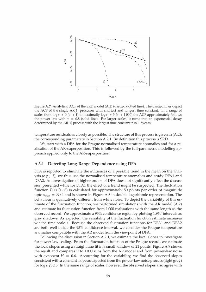
0 1 2 3

1e−

061e

−04

1e−

021e

+00

log10 s

AC

F

a1s

a3s

s−0.8

3 AR[1]

Figure A.7: Analytical ACF of the SRD model (A.2) (dashed dotted line). The dashed lines depictthe ACF of the single AR[1] processes with shortest and longest time constant. In a range ofscales from log s ≈ 0 (s ≈ 1) to maximally log s ≈ 3 (s ≈ 1 000) the ACF approximately followsthe power law with γ = 0.8 (solid line). For larger scales, it turns into an exponential decaydetermined by the AR[1] process with the largest time constant τ ≈ 1.5years.

temperature residuals as closely as possible. The structure of this process is given in (A.2),the corresponding parameters in Section A.2.1. By definition this process is SRD.

We start with a DFA for the Prague normalised temperature anomalies and for a re-alisation of the AR-superposition. This is followed by the full-parametric modelling ap-proach applied only to the AR-superposition.

A.3.1 Detecting Long-Range Dependence using DFA

DFA is reported to eliminate the influences of a possible trend in the mean on the anal-ysis (e.g., ?), we thus use the normalised temperature anomalies and study DFA1 andDFA2. An investigation of higher orders of DFA does not significantly affect the discus-sion presented while for DFA1 the effect of a trend might be suspected. The fluctuationfunction F(s) (1.68) is calculated for approximately 50 points per order of magnitudeupto smax = N/4 and is shown in Figure A.8 in double logarithmic representation. Thebehaviour is qualitatively different from white noise. To depict the variability of this es-timate of the fluctuation function, we performed simulations with the AR model (A.2)and estimate its fluctuation function from 1 000 realisations with the same length as theobserved record. We approximate a 95% confidence region by plotting 1.96σ intervals asgrey shadows. As expected, the variability of the fluctuation function estimate increaseswit the time scale s. Because the observed fluctuation functions for DFA1 and DFA2are both well inside the 95% confidence interval, we consider the Prague temperatureanomalies compatible with the AR model from the viewpoint of DFA.

Following the discussion in Section A.2.1, we estimate the local slopes to investigatefor power-law scaling. From the fluctuation function of the Prague record, we estimatethe local slopes using a straight line fit in a small window of 21 points. Figure A.9 showsthe result and compares it to 1 000 runs from the AR model and from power-law noisewith exponent H = 0.6. Accounting for the variability, we find the observed slopesconsistent with a constant slope as expected from the power-law noise process (light grey)for log s & 2.5. In the same range of scales, however, the observed slopes also agree with

59

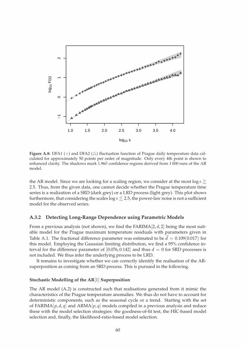
1.0 1.5 2.0 2.5 3.0 3.5 4.0

−1

01

2

log10 s

log 1

0 F

(s)

Figure A.8: DFA1 (+) and DFA2 () fluctuation function of Prague daily temperature data cal-culated for approximately 50 points per order of magnitude. Only every 4th point is shown toenhanced clarity. The shadows mark 1.96σ confidence regions derived from 1 000 runs of the ARmodel.

the AR model. Since we are looking for a scaling region, we consider at the most log s &2.5. Thus, from the given data, one cannot decide whether the Prague temperature timeseries is a realization of a SRD (dark grey) or a LRD process (light grey). This plot showsfurthermore, that considering the scales log s . 2.5, the power-law noise is not a sufficientmodel for the observed series.

A.3.2 Detecting Long-Range Dependence using Parametric Models

From a previous analysis (not shown), we find the FARIMA[2, d, 2] being the most suit-able model for the Prague maximum temperature residuals with parameters given in

Table A.1. The fractional difference parameter was estimated to be d = 0.109(0.017) forthis model. Employing the Gaussian limiting distribution, we find a 95% confidence in-terval for the difference parameter of [0.076, 0.142] and thus d = 0 for SRD processes isnot included. We thus infer the underlying process to be LRD.

It remains to investigate whether we can correctly identify the realisation of the AR-superposition as coming from an SRD process. This is pursued in the following.

Stochastic Modelling of the AR[1] Superposition

The AR model (A.2) is constructed such that realisations generated from it mimic thecharacteristics of the Prague temperature anomalies. We thus do not have to account fordeterministic components, such as the seasonal cycle or a trend. Starting with the setof FARIMA[p, d, q] and ARMA[p, q] models compiled in a previous analysis and reducethese with the model selection strategies: the goodness-of-fit test, the HIC-based modelselection and, finally, the likelihood-ratio-based model selection.

60

1.5 2.0 2.5 3.0 3.5 4.0

0.4

0.6

0.8

1.0

1.2

log10 s

α

(a)

1.5 2.0 2.5 3.0 3.5 4.0

0.4

0.6

0.8

1.0

1.2

log10 s

α

(b)

Figure A.9: Local slopes α (or H) of the fluctuation functions plotted in Figure A.8 for DFA1 (a)and DFA2 (b) of the Prague daily temperature data. The dotted lines border the 1.96σ confidenceregions of the short-range correlated model (A.2) (dark shadow), the dashed lines those of thelong-memory model with H = 0.6 (light shadow).

61

Parameter FARIMA[2, d, 2] ARMA[5, 3] ARMA[8, 1]d 0.109(0.017) – –a1 1.210(0.066) 1.548(0.275) 1.762(0.012)a2 −0.332(0.042) −0.139(0.544) −0.879(0.012)a3 – −0.679(0.368) 0.145(0.008)a4 – 0.314(0.116) −0.035(0.008)a5 – −0.050(0.019) 0.005(0.008)a6 – – −0.003(0.008)a7 – – 0.002(0.008)a8 – – −0.005(0.004)b1 −0.513(0.057) −0.741(0.275) −0.955(0.011)b2 −0.106(0.007) −0.567(0.326) –b3 – 0.342(0.095) –

p-val 0.074 0.071 0.075

Table A.1: Maximum likelihood parameter estimates and asymptotic standard deviation in paren-theses for the FARIMA[2, d, 2], ARMA[5, 3] and ARMA[8, 1] process obtained from the Praguetemperature residuals. The last line gives the p-values of the goodness-of-fit test.

Goodness-of-fit On the basis of the goodness-of-fit test (2.4) applied to the before men-tioned set of models we reject only the FD (FARIMA[0, d, 0]) model on a 5%-level of sig-nificance.

HIC Model Selection Figure A.10 depicts the HIC values for the models considered.It is striking that for the most cases the ARMA[p, q] model has a smaller HIC than thecorresponding FARIMA[p, d, q] model. Investigating the fractional difference parameterfor the latter models (Table A.2) reveals that besides FARIMA[1, d, 0], FARIMA[1, d, 1] andFARIMA[2, d, 0] all estimates are compatible with the d = 0 within one (or, in one case,1.96) standard deviation. We retain these models, as well as ARMA[p, q] models withorders (p, q) ∈ (2, 1), (2, 2), (3, 1), (3, 2). Keeping other FARIMA[p, d, q] models is notmeaningful, because their fractional difference parameter is compatible with zero andthus they are equivalent to the corresponding ARMA[p, q] processes.

Likelihood-Ratio Test With a likelihood-ratio test, we investigate whether the threemodels with a non-trivial fractional difference parameter are admissible simplifications ofthe FARIMA[2, d, 1], the simplest models with trivial difference parameter. The p-valuesin Table A.3 (right) reveal that we can reject this hypothesis for all three cases on a 5%-level (or even 1%-level) of significance. This implies, that there is no evidence for a LRDprocess underlying this data series.

Among the ARMA[p, q] models, we find the ARMA[2, 2] and ARMA[3, 1] as admissi-ble simplifications of the ARMA[3, 2] (Table A.3, left, lines 1 and 2). Both models can befurther simplified by ARMA[2, 1] (lines 3 and 4). The latter is the most suitable model outof the canon we started with for the realisation of the AR-superposition (A.2).

Using the full-parametric modelling approach we are thus able to correctly identifythe realisation of a superposition of three AR[1] processes as coming from an SRD process.This was not possible by means of DFA. The original model, a superposition of AR[1]processes (A.2), was not included in the model canon we used to describe the exampleseries with. However, such a superposition can be well approximated with ARMA[p, q]processes.

62

1390

6013

9080

1391

00

Model Order [p,q]

HIC

[0,0

][1

,0]

[1,1

][2

,0]

[2,1

][2

,2]

[3,0

][3

,1]

[3,2

][3

,3]

[4,0

][4

,1]

[4,2

][4

,3]

[4,4

][5

,0]

[5,1

][5

,2]

[5,3

][5

,4]

[5,5

][6

,0]

[6,1

][6

,2]

[6,3

][6

,4]

[6,5

][6

,6]

[7,0

][7

,1]

[7,2

][7

,3]

[7,4

][7

,5]

[7,6

][7

,7]

[8,0

][8

,1]

[8,2

][8

,3]

[8,4

][8

,5]

[8,6

][8

,7]

ARMA[p,q]FARIMA[p,d,q]

Figure A.10: HIC for various ARMA[p, q] (green) and FARIMA[p, d, q] (red) models fitted to real-isation of the AR model (A.2) The model orders [p, q] are plotted along the abscissa.

Model d(σd)

[1, d, 0] 0.148(0.010)[1, d, 1] 0.158(0.011)[2, d, 0] 0.160(0.011)[2, d, 1] 0.000(0.015)[2, d, 2] 0.000(0.037)[3, d, 1] 0.000(0.037)[3, d, 2] 0.012(0.017)[4, d, 1] 0.000(0.040)[3, d, 3] 0.028(0.038)[4, d, 2] 0.027(0.038)[5, d, 1] 0.000(0.042)[4, d, 3] 0.023(0.022)[5, d, 2] 0.000(0.041)

Table A.2: Estimates and asymptotic standard deviation of the fractional difference parameterobtained for the FARIMA[p, d, q] models with smallest HIC.

63

ARMA[p, q]Model f Model g p-val

1 [3, 2] [2, 2] 12 [3, 2] [3, 1] 0.7133 [2, 2] [2, 1] 0.5844 [3, 1] [2, 1] 0.939

FARIMA[p, d, q]Model f Model g p-val

1 [2, d, 1] [2, d, 0] <0.0012 [2, d, 1] [1, d, 1] <0.0013 [2, d, 1] [1, d, 0] <0.001

Table A.3: p-values for a likelihood-ratio test of model g being an admissible simplification ofmodel f for ARMA[p, q] and FARIMA[p, d, q] models of the realisation stemming from the AR[1]-superposition (A.2).

A.4 Summary

In a simulation study, we investigated bias and variance for a DFA-based estimator for theHurst exponent using realisations of power-law noise. These properties of the estimatorare not only influenced by the time series length but also by the Hurst exponent of theunderlying process. Without knowledge about bias and variance, inference about theHurst exponent cannot be made.

We further considered the inference of LRD by means of DFA with respect to thenotions of sensitivity and specificity. The inference of a LRD process underlying a giventime series requires not only to show compatibility of the data with a LRD process ina certain range of scales. Furthermore, other possible correlation structures, especiallySRD, have to be excluded.

Power-law like behaviour in some range of scales of the DFA fluctuation functionalone is frequently taken as evidence for LRD. To reliably infer power-law scaling, itmust not be assumed but has to be established. This can be done by estimating localslopes and investigating them for constancy in a sufficient range. However, finite datasets bring along natural variability. To decide, if a fluctuating estimation of the slopehas to be considered as being constant, we calculated empirical confidence intervals for aLRD and a simple SRD model.

Discussing typical difficulties of interpreting DFA results, we note that scaling cannotbe concluded from a straight line fit to the fluctuation function in a log-log representation.Additionally, we show that a local slope estimate HDFAn > 0.5 for large scales does notnecessarily imply long-memory. If the length of the time series is not sufficiently largecompared to the time scales involved, also for SRD processes HDFAn = 0.5 may not bereached. Finally, we demonstrated, that it is not valid to conclude from a finite scalingregion of the fluctuation function to an equivalent scaling region of the ACF.

With the Prague temperature anomalies and a corresponding artificial series from aSRD process, we exemplify the problems and pitfalls discussed. Using DFA we couldnot discriminate the Prague record from the artificial series. Furthermore, by means of alog-log plot, we classify the underlying process of both series as LRD, leading to a falsepositive result for the SRD process. A reliable identification was possible with the full-parametric ansatz (Section 3.4).

Because it is always possible to find and SRD process to describe a finite set of data,some criterion is needed to evaluate the performance of the description taking the com-plexity of the model into account. We thus approach the problem of distinguishing SRDand LRD processes on the basis of a realisation of a parametric modelling point of viewdeveloped in Chapter 3.

64

Appendix B

Long-Range Dependence – Effects,Methods, Mechanisms

A simple example to illustrate the effect of long-range dependence on the estimation ofstatistical quantities is illustrated in the first section. This is followed by some physicalexplanations of the phenomenon. Further, we describe the log-periodogram regressionand the rescaled-range statistic as methods to quantify LRD. This is followed by introduc-ing two LRD specific statistics which can be used as further criteria for the simulation-based model selection described in Section 2.3.2. These statistics are based on the log-periodogram regression and on DFA. Subsequently, we describe the generation of anartificial series, which is used as a challenging example to illustrate the LRD detectionstrategies described in Chapter 3.

B.1 Effects of Long-Range Dependence

We illustrate the effect of LRD on statistical quantities estimated from a realisation of astochastic process with a simple example: consider the arithmetic mean X = N−1 ∑

Nt=1 Xt

as an estimator for the the expectation value µ, i.e. µ = X. A basic result in statistics isthe decrease in variance of the arithmetic mean with an increasing sample size N. Forrandom variables Xt, identically distributed with expectation value µ and variance σ2,the variance of the arithmetic mean X can be calculated as (?)

var(X) =σ2

N2

N

∑s,t=1

cor(Xs, Xt). (B.1)

For independent Xt with cor(Xs, Xt) = 0 for s 6= t this reduces to the well known resultvar(X) = σ2/N. In case of a dependent process Xt, the calculation of var(X) requires toconsider the ACF ρ(τ). For a weakly stationary process, we find

var(X) =σ2

N

[1 + 2

N−1

∑τ=1

(1 − τ

N

)ρ(τ)

]. (B.2)

In case of a more specific description of the stationary process equation (B.2) can be fur-ther simplified. It is instructive to consider two examples: an autoregressive process(AR[1], cf. Section 1.2.1), as a prominent representative of a SRD processes, and a LRDprocess, specified only by the limiting behaviour (1.21).

65

Example 1: Short-Range Dependence

With the autocorrelation function for an AR[1] process ρ(τ) = aτ with |a| < 1 as de-scribed in Section 1.2.1, equation (B.2) reads

var(X) =σ2

N

[1 + 2

N−1

∑τ=1

(1 − k

N

)aτ

], (B.3)

which in the limit of large N reduces to

var(X) ≈ σ2

N

[1 +

2a

1 − a

]=

σ2

Nca, (B.4)

with ca = 1 + 2a1−a being a constant depending on the AR coefficient. In this case the

variance of the mean decreases at the same rate as for uncorrelated data, namely var(X) ∝

N−1, but with a different constant.

Example 2: Long-Range Dependence

For a process with an algebraically decaying ACF, ρ(τ) ∝ τ−γ with γ ∈ (0, 1), for largelags the sum in (1.20) does not converge to a constant value. It behaves instead as

N−1

∑τ=−(N−1)

ρ(τ) ∝ N1−γ, (B.5)

which in turn leads to

var(X) ∝σ2

Nγ. (B.6)

Because γ < 1, this algebraic decay of the variance of the mean is slower than the expo-nential decay for uncorrelated or short-range correlated processes (?).

These examples point towards the pivotal difference in records from LRD and SRDprocesses: given a sample of length N, for SRD processes the mean value can be estimatedwith the variance decreasing as 1/N, while for a LRD process the variance of this estima-tor decreases only with 1/Nγ and is thus in general larger. Consequently, the uncertaintyof statistical measures inferred from records of LRD processes is larger than in the caseof SRD. Statistical measures which are affected are, e.g., regression coefficients (?), semi-parametric trend estimates (??) or quantiles estimated from the frequency distribution(?). The latter effect is of tremendous importance in extreme value statistics, e.g., whensetting design values for hydraulic constructions as dams, bridges or dykes (?). The ef-fect on regression coefficients is relevant with respect to trend detection, a highly debatedtopic in the early years of climate change research: assuming a LRD process underlyingtemperature records allows small trends to “hide” in the low frequency variability andrenders detection more difficult (?). It is thus of considerable importance to reliably detectan underlying LRD process. Having discovered that a frequently used heuristic approachis prone to falsely detect LRD (Section A.2; ?), the development of a different approach tothe detection of LRD based on parametric modelling and model selection is suggested inChapter 3.

66

B.2 Physical Explanations of the Phenomenon

In the time after ?, various explanations or descriptions of the Hurst phenomenon emerged.In the 1960s Mandelbrot suggested increments of self-similar processes to describe thiseffect (cf. Section 1.2.2). The aggregation of processes with different time scales was sug-gested by ?. Certain types of instationarities being held responsible for the phenomenonwere discussed by ?. The latter two approaches are discussed in brevity in the following.An extensive overview about the Hurst phenomenon from a hydrological perspectivehas been given by ??.

Aggregation of Processes with Different Characteristic Time Scales

? showed that it is possible to preserve the Hurst phenomenon (in particular the rescaledrange statistic, Section B.3.1) for a finite time series with conventional linear stochasticmodels (cf. Section 1.2.1). ? showed that a superposition of n first order autoregressiveprocesses (AR[1], Section 1.2.1) lead to a long-range dependent process in the limit oflarge n. The parameters a and ση of these processes (1.23) have to be independent ran-dom variables following a beta distribution. Physically, the parameter a is related to therelaxation time of the process. This implies that a suitable superposition of relaxationswith different characteristic time scales can evoke the Hurst phenomenon.

Instationarities

Instationarities in the empirical series, such as a trend in the mean, have been held re-sponsible for the Hurst phenomenon (e.g., ?). The latter motivated the development ofmethods supposed to eliminate the influence of trends, like the detrended fluctuationanalysis (DFA) described in Section 1.3.3.

Other Explanations

Further variants of models showing the Hurst phenomenon are proposed for example by?? and ?. Especially interesting is the idea of ?. He suggests that heteroscedasticity, i.e. anon-homogeneous variance, might also account for the phenomenon. Heteroscedasticitycan also be found in run-off records (?).

B.3 Further Heuristic and Semi-Parametric Methods to Quantify

LRD

B.3.1 Rescaled Adjusted Range

? studied the flow of the Nile using the rescaled adjusted range statistic (R/S). Consider theinflow Xt at time t, the cumulative inflow Yt = ∑

ti=1 Xi and the mean Xt,s = 1/s ∑

t+si=t+1 Xt.

The rescaled adjusted range is then

R/S = E

[R(t, s)

S(t, s)

]

t

, (B.7)

with

R(t, s) = max0≤i≤s

[Yt+i − Yt −i

s(Yt+s −Yt)]− min

0≤i≤s[Yt+i − Yt −

i

s(Yt+s − Yt)],

67

and

S(t, s) =

√√√√s−1t+s

∑i=t+1

(Xi − Xt,s)2.

For large s, a plot of log R/S versus log s is approximately scattered around a straight linewith slope H (?).

The R/S statistic was refined by Mandelbrot and others (e.g., ???). Later ? derivedthe asymptotic behaviour for R/S for short-range and long-range dependent processes.The latter can be described following ?:

For Xt such that X2t is ergodic and t−

12 ∑

tk=1 Xk converges weakly to Brownian motion

as t → ∞ then for s → ∞ and Q(t, s) = R(t, s)/S(t, s)

s−12 Q(t, s)

d→ ξ, (B.8)

with ξ being a nondegenerate random variable.It remains open for which range of s the described asymptotic behaviour starts and

what the confidence interval of the estimate is. For a finite sample the distribution of His neither normal nor symmetric. All this makes inference about the value of H difficult.

In fact, in the presence of unanticipated high frequency behaviour, ? noticed the in-validity of a test for H = 0.5, i.e. uncorrelated series. Based on the asymptotic theory forthe R/S statistic by ? this null hypothesis is rejected too often. ? developed a correctedstatistic accounting for a wide range of high frequency components.

The R/S statistic was not designed to discriminate between short-range and long-range dependent processes, it is rather a tool to measure the Hurst exponent H in situa-tions where the region of asymptotic behaviour is known. This is a severe shortcomingencountered also in the description of further heuristic approach such as DFA (cf. Ap-pendix A). In many fields where long-range dependence is to be taken into account, suchas geophysics or econometrics, also high frequency components are present. They needto be accounted for in order to obtain reliable results.

B.3.2 Log-Periodogram Regression

In case a full-parametric description of the spectral density (Chapter 3) cannot be achieveor is not pursued. The fractional difference parameter can be estimated using a semi-parametric approach in the spectral domain. Referring to a definition of LRD (1.22), thespectral density S(ω) close to the origin behaves as

S(ω) ∝ c f |ω|−β, |ω| → 0. [1.22]

The exponent β can be related to the fractional difference parameter d by β = 2d. Takingthe logarithm on both sides, the equation motivates a regression approach to estimate βor, equivalently, the fractional difference parameter d. Consider

log I(ωj) ≈ log c f − β log |ωj|+ uj, (B.9)

with a positive constant c f and j = l, . . . , m.

The GPH Estimator

? (GPH) were the first to suggest the estimation of a parameter quantifying the long-rangedependence (either β or d) using this kind of regression. However, instead of log ωj they

68

considered log|1 − eiωj | as regressor motivated by the exact form of the spectral densityfor fractional ARIMA processes (1.50). Furthermore, they included frequencies ωj in the

regression starting with j = 0 to obtain the estimate dlp = β/2. ? argued for the followingGaussian limiting distribution of this estimator:

m1/2(dlp − d)d→ N

(0,

π2

24

). (B.10)

With this result, they provided a simple way to approximate confidence intervals andcarry out hypothesis testing (cf. Section 2.1.1).

However, ? showed that their arguments do not hold. Mainly because the residualsuj cannot be considered as asymptotically independent or homoscedastic. Despite this,the desired limiting distribution (B.10) could be established by ? for Gaussian processesusing log ωj as regressor as suggested in (B.9) and by trimming out the smallest frequencyωj (?). This result was generalised to linear processes by ?.

Semi-Parametric Whittle-Estimation

An even more efficient estimator was suggested by ? with the limiting distribution pro-vided by ?. It is essentially based on Whittle estimation of the model S(ω) = Cω−2d forthe first m frequencies:

dK = arg mind

log

[1

m

m

∑j=1

I(ωj)

ω−2dj

]− 2d

m

m

∑j=1

log ωj

. (B.11)

Under milder regularity conditions than those required for (B.9), the limiting distributionis given by

m1/2(dk − d)d→ N

(0,

1

4

), (B.12)

having a smaller variance and leading thus to a more efficient estimator. Different from

(B.9) no closed form for dk can be given. The estimate has to be obtained numerically inthe same way as described for the full-parametric Whittle estimator in Section 1.3.2.

Bandwidth Choice and Related Approaches

For dK, as well as for dlp a bandwidth m has to be chosen for the estimation. A brief reviewon various approaches on the choice of an optimal bandwidth is given in ?. ? discuss anoptimal choice of the bandwidth in the sense of a bias-variance trade-off.

The log-periodogram regression for the non-stationary domain d > 0.5 has been dis-cussed by ?. A similar approach to estimate the long-range dependence parameter usingwavelet analysis is described by ? and ?.

Combining Log-Periodogram Regression and ARMA[p, q] Parameter Estimation

It is conceivable to estimate the (fractional) difference parameter d and the autoregres-sive moving average parameters ai and bj separately. In the early days of ARIMA[p, d, q]processes (with d ∈ N), the estimation for integer differences has been carried out byheuristic methods and for the following inference about the AR and MA parameters dwas assumed to be known (?). For fractional differences d ∈ R, the first step can be

69

carried out using, e.g., the log-periodogram regression; the inference about ARMA pa-rameters, for example, by maximum likelihood. For the log-periodogram regression it ispossible to specify a confidence interval for the estimate of d in contrast to the heuristicmethods of estimating the integer difference paramters. However, the influence of esti-mating d on the estimation of the autoregressive and moving average parameters is notaccounted for. In a combined approach, i.e. simultaneous estimation of the parameters d,ai and bj, this influence can be quantified via the covariance matrix V of the parametervector θ (Section 1.3.1).

B.4 Specific Test Statistics for Model Selection

In this section, we evaluate two statistics which can be used in the simulation-basedmodel selection described in Section 2.3.2. Being especially interested in the low fre-quency behaviour, we investigate the performance of the log-periodogram regression(Section B.3.2) and the DFA (Section 1.3.3) as further model selection criteria. For bothapproaches one has to choose an appropriate bandwidth for the straight line fit. We usethis free parameter to optimise the power (Section 2.3.3), i.e. the separation of the twodistributions resulting from the simulations. For both criteria, we calculate p-values andpower and try to identify an optimal bandwidth. It turned out to be also instructive toexamine the dependence of the estimates on the bandwidth.

As an example, we consider the setting introduced in Section 3: a realisation of anARMA[3, 2] process (Section 3.1; Appendix B.5) and models FAR[1] and ARMA[3, 2]. Weestimate the model parameters from the realisation and obtain thus two fully specifiedmodels. These two models are used to generate two ensembles of realisations. For all

ensemble members the estimates dlp (or dDFA, Section 1.3.3) are calculated. The esti-mate from the observed series is then compared to the distribution obtained from theensembles. The p-values and power can be obtained in the same way as described forthe likelihood-ratio (cf. Section 2.3.2). For better readability, we denote the ARMA[3, 2]model as f and the corresponding hypothesis as H f , analogously g represents the FAR[1]model.

B.4.1 Log-Periodogram Regression

Bandwidth-Dependence of the Power

The power for a critical nominal level of α = 0.05 as a function of the bandwidth of thelinear fit is shown in Figure B.1 (left) for testing H f against Hg (green) and vice versa(red). In both cases a maximum power is achieved for a bandwidths 0 < ω < ω1 =0.0021: pow f (g, 0.05) = 0.851 and powg( f , 0.05) = 0.836. Thus this test is not as powerful

as the one based on the likelihood-ratio which exhibits a power pow > 0.9 for bothtest situations (Section 3.4.1). The distribution functions for the ensembles of fractionaldifference parameter estimates for the two hypothesis are shown in Figure B.1 (right) forthe bandwidth with maximal power. The estimate obtained for the “observed” series isdepicted as a vertical bar and is located in the gap between the two critical regions. Thus,neither hypothesis can be rejected in this example.

70

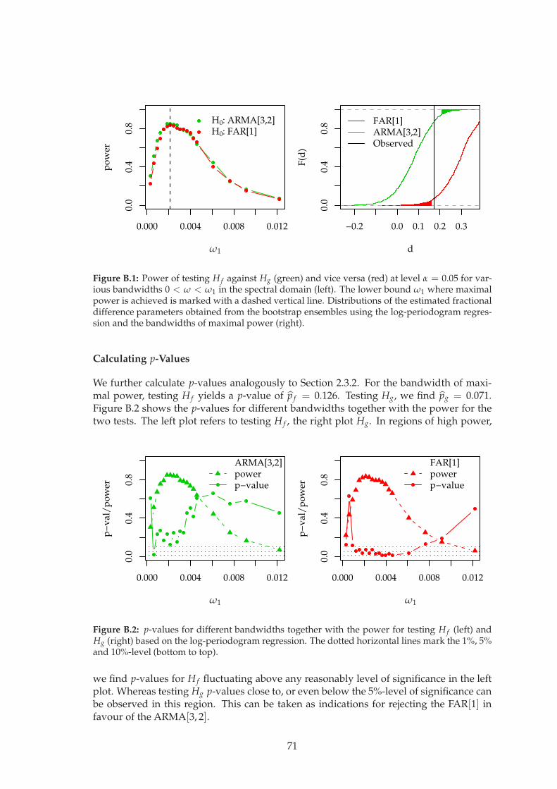
0.000 0.004 0.008 0.012

0.0

0.4

0.8

po

wer

H0: ARMA[3,2]H0: FAR[1]

ω1

−0.2 0.0 0.1 0.2 0.3

0.0

0.4

0.8

d

F(d

)

FAR[1]ARMA[3,2]Observed

Figure B.1: Power of testing H f against Hg (green) and vice versa (red) at level α = 0.05 for var-ious bandwidths 0 < ω < ω1 in the spectral domain (left). The lower bound ω1 where maximalpower is achieved is marked with a dashed vertical line. Distributions of the estimated fractionaldifference parameters obtained from the bootstrap ensembles using the log-periodogram regres-sion and the bandwidths of maximal power (right).

Calculating p-Values

We further calculate p-values analogously to Section 2.3.2. For the bandwidth of maxi-mal power, testing H f yields a p-value of p f = 0.126. Testing Hg, we find pg = 0.071.Figure B.2 shows the p-values for different bandwidths together with the power for thetwo tests. The left plot refers to testing H f , the right plot Hg. In regions of high power,

0.000 0.004 0.008 0.012

0.0

0.4

0.8

p−

val

/p

ow

er

ARMA[3,2]powerp−value

ω1

0.000 0.004 0.008 0.012

0.0

0.4

0.8

p−

val

/p

ow

er

FAR[1]powerp−value

ω1

Figure B.2: p-values for different bandwidths together with the power for testing H f (left) andHg (right) based on the log-periodogram regression. The dotted horizontal lines mark the 1%, 5%and 10%-level (bottom to top).

we find p-values for H f fluctuating above any reasonably level of significance in the leftplot. Whereas testing Hg p-values close to, or even below the 5%-level of significance canbe observed in this region. This can be taken as indications for rejecting the FAR[1] infavour of the ARMA[3, 2].

71

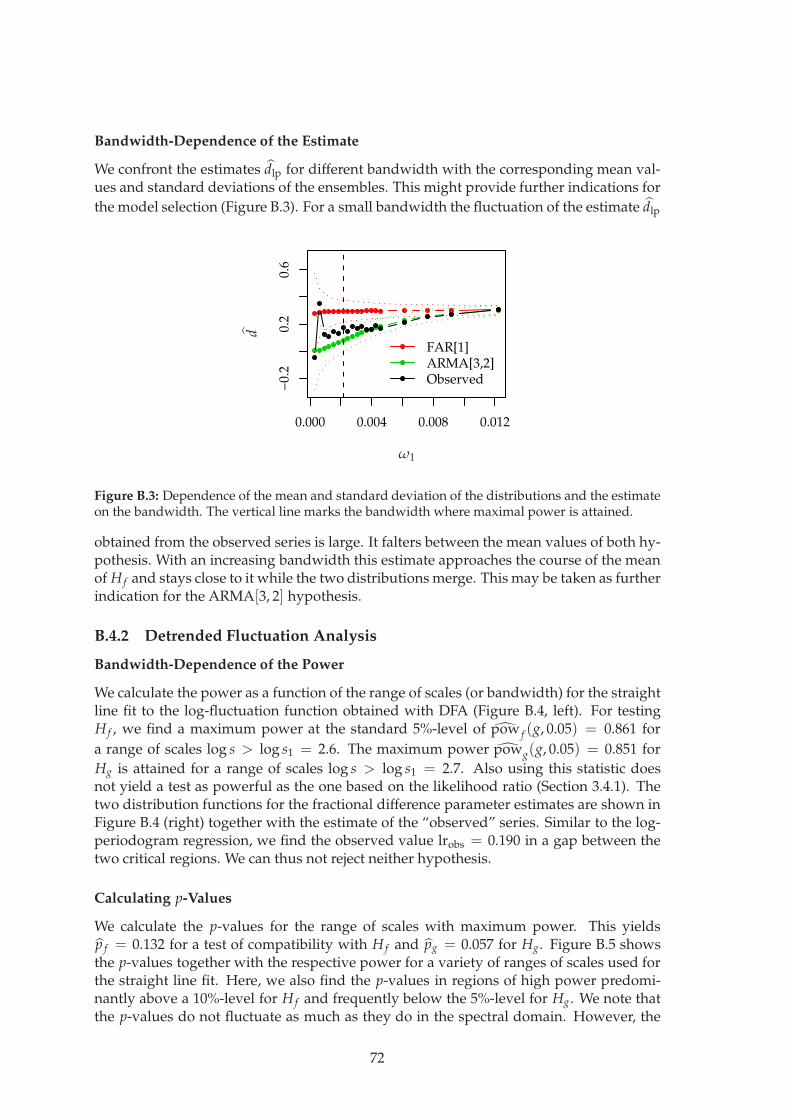
Bandwidth-Dependence of the Estimate

We confront the estimates dlp for different bandwidth with the corresponding mean val-ues and standard deviations of the ensembles. This might provide further indications for

the model selection (Figure B.3). For a small bandwidth the fluctuation of the estimate dlp

0.000 0.004 0.008 0.012

−0.

20.

20.

6

FAR[1]ARMA[3,2]Observed

ω1

d

Figure B.3: Dependence of the mean and standard deviation of the distributions and the estimateon the bandwidth. The vertical line marks the bandwidth where maximal power is attained.

obtained from the observed series is large. It falters between the mean values of both hy-pothesis. With an increasing bandwidth this estimate approaches the course of the meanof H f and stays close to it while the two distributions merge. This may be taken as furtherindication for the ARMA[3, 2] hypothesis.

B.4.2 Detrended Fluctuation Analysis

Bandwidth-Dependence of the Power

We calculate the power as a function of the range of scales (or bandwidth) for the straightline fit to the log-fluctuation function obtained with DFA (Figure B.4, left). For testingH f , we find a maximum power at the standard 5%-level of pow f (g, 0.05) = 0.861 for

a range of scales log s > log s1 = 2.6. The maximum power powg(g, 0.05) = 0.851 for

Hg is attained for a range of scales log s > log s1 = 2.7. Also using this statistic doesnot yield a test as powerful as the one based on the likelihood ratio (Section 3.4.1). Thetwo distribution functions for the fractional difference parameter estimates are shown inFigure B.4 (right) together with the estimate of the “observed” series. Similar to the log-periodogram regression, we find the observed value lrobs = 0.190 in a gap between thetwo critical regions. We can thus not reject neither hypothesis.

Calculating p-Values

We calculate the p-values for the range of scales with maximum power. This yieldsp f = 0.132 for a test of compatibility with H f and pg = 0.057 for Hg. Figure B.5 showsthe p-values together with the respective power for a variety of ranges of scales used forthe straight line fit. Here, we also find the p-values in regions of high power predomi-nantly above a 10%-level for H f and frequently below the 5%-level for Hg. We note thatthe p-values do not fluctuate as much as they do in the spectral domain. However, the

72

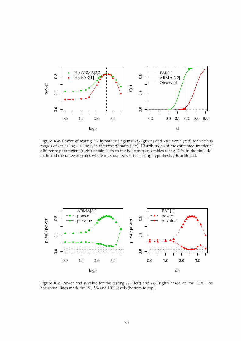
0.0 1.0 2.0 3.0

0.0

0.4

0.8

log s

po

wer

H0: ARMA[3,2]H0: FAR[1]

Lag [years]

−0.2 0.0 0.1 0.2 0.3 0.4

0.0

0.4

0.8

dF

(d)

FAR[1]ARMA[3,2]Observed

Figure B.4: Power of testing H f hypothesis against Hg (green) and vice versa (red) for variousranges of scales log s > log s1 in the time domain (left). Distributions of the estimated fractionaldifference parameters (right) obtained from the bootstrap ensembles using DFA in the time do-main and the range of scales where maximal power for testing hypothesis f is achieved.

0.0 1.0 2.0 3.0

0.0

0.4

0.8

log s

p−

val

/p

ow

er

ARMA[3,2]powerp−value

0.0 1.0 2.0 3.0

0.0

0.4

0.8

p−

val

/p

ow

er

FAR[1]powerp−value

ω1

Figure B.5: Power and p-value for the testing H f (left) and Hg (right) based on the DFA. Thehorizontal lines mark the 1%, 5% and 10%-levels (bottom to top).

73

difference to the 10%-level in the case of model f and the difference to the 5%-level incase of model g are also less pronounced.

Bandwidth-Dependence of the Estimate

The p-values changing with the range of scales used for the fit (Figure B.6) indicate that

the estimates dDFA rather follows the mean of H f . The distinction is not as clear as it isin the case of the log-periodogram regression in Figure B.3. This, as well as the p-values

0.0 1.0 2.0 3.0

0.0

0.2

0.4

log s

FAR[1]ARMA[3,2]Observed

d

Figure B.6: Development of the mean and standard deviation of the hypothesis with varyingrange of scales for DFA. The vertical line marks the range where maximal power is attained.

obtained in the previous paragraph, may be taken as a hint to favour the ARMA[3, 2].

B.5 Constructing the Example Process – Detailed Description

The aim of this section is to generate challenging example series for testing the strategiesto detect LRD (Chapter 3). We start with a realisation xii=1,...,N of an FARIMA[1, d, 0] (or,for short, FAR[1]) process with parameters a1 = 0.7, d = 0.3 and length N = 215 = 32 768.The length and the parameters are chosen such that they are plausible for river run-off,the context which we are going to apply this detection strategy in. A realisation of thisprocess is shown in the time and spectral domain in Figure B.7. Now, we aim to find aSRD model which describes this realisation well. We expect such a SRD model to producerealisations which will be difficult to discriminate from realisations of the original LRDprocess.

Selecting an ARMA[p, q] model for the FAR[1] Realisation

We fit various ARMA[p, q] models with p < 4 and q < min(p, 2) and compare the valuesfor the Hannan-Quinn criterion (HIC) (cf. Section 2.2.2) in Figure B.8. The smallest valueis attained for the ARMA[3, 2] process. Very close to this value, separated by less than 2units, we find the ARMA[4, 1] model. About 4 units more yields the HIC for ARMA[4, 2].Note, that at this stage we do not necessarily intent to find one “best model”. We arerather looking for some ARMA[p, q] model representing the given FAR[1] realisation wellenough, such that realisations can be easily mistaken for coming from an LRD process.

74

0 1000 3000 5000

−5

05

FAR[1]Index

Dat

a

Lag [years]

5e−04 1e−02 5e−01

1e−

051e

−01

1e+

03

FAR[1]P

ow

erω

Figure B.7: Realisation of a FAR[1] process with parameters a1 = 0.7, d = 0.3 and length N =32 768, in the time domain (left, only the first 5 000 data points) and in the frequency domain(right).

9310

093

300

9350

0

Best HIC : ARMA[3,2]Model Order [p,q]

HIC

[1,0

]

[1,1

]

[2,0

]

[2,1

]

[2,2

]

[3,0

]

[3,1

]

[3,2

]

[4,0

]

[4,1

]

[4,2

]

Figure B.8: Multiple ARMA[p, q] fits to the realisation of the FAR[1] process shown in FigureB.7. The plot shows the values for the Hannan-Quinn criterion (HIC) for models with the order1 < p < 4 and 0 < q < min(p, 2).

75

There is no need to discriminate between these three similar performing models. For ourupcoming example, we choose the ARMA[3, 2] process with parameters a1 = 2.178, a2 =−1.448, a3 = 0.309, b1 = −1.184 and b2 = 0.218. The model is completely specified andwe can now generate a realisation, which are used to study the detection strategies forLRD in Chapter 3.

76