spectral analysis of the flow behavior of big spring
TRANSCRIPT

UNLV Theses, Dissertations, Professional Papers, and Capstones
12-1993
Spectral analysis of the flow behavior of Big Spring, Kings Canyon Spectral analysis of the flow behavior of Big Spring, Kings Canyon
National Park, California National Park, California
Linda Urzendowski
Follow this and additional works at: https://digitalscholarship.unlv.edu/thesesdissertations
Part of the Geology Commons, and the Hydrology Commons
Repository Citation Repository Citation Urzendowski, Linda, "Spectral analysis of the flow behavior of Big Spring, Kings Canyon National Park, California" (1993). UNLV Theses, Dissertations, Professional Papers, and Capstones. 1445. http://dx.doi.org/10.34917/3433935
This Thesis is protected by copyright and/or related rights. It has been brought to you by Digital Scholarship@UNLV with permission from the rights-holder(s). You are free to use this Thesis in any way that is permitted by the copyright and related rights legislation that applies to your use. For other uses you need to obtain permission from the rights-holder(s) directly, unless additional rights are indicated by a Creative Commons license in the record and/or on the work itself. This Thesis has been accepted for inclusion in UNLV Theses, Dissertations, Professional Papers, and Capstones by an authorized administrator of Digital Scholarship@UNLV. For more information, please contact [email protected].

SPECTRAL ANALYSIS OF THE
FLOW BEHAVIOR OF BIG SPRING,
KINGS CANYON NATIONAL PARK, CALIFORNIA
by
Linda Urzendowski
A thesis submitted in partial fulfillment of the requirements for the degree of
Master of Science
in
Geoscience
Department of Geoscience University of Nevada, Las Vegas
December 1993

The Thesis of Linda Urzendowski for the degree of Master of Science in Geoscience is approved.
9/.27 )f.:? Chairp~son, John W:Hi3ss, Ph.D. / I
f/?z/13 Examining Committee Member, Frederick W. Bachhuber, Ph.D.
Graduate Faculty Representative, Richard L. Titus, Ph.D.
Dean of the Graduate College, Ronald W. Smith, Ph.D.
University of Nevada, Las Vegas December 1993
ii

ABSTRACT
Big Spring, the resurgence of a karst aquifer in the Lilburn Cave system
(Kings Canyon National Park, California), displays the uncommon phenomena
of ebb and flow discharge during periods of high runoff. Time-series,
hydrograph and spectral analyses (power spectra, transfer and kernel functions)
of the stage and discharge data, chemistry and sediment analyses, and a
bench-scale model were combined to elucidate the internal hydrology of this
cave-spring system.
Time-series observations revealed two distinct types of flow patterns at
Big Spring during the high runoff season (usually February through early June).
The first is an ebb and flow, 180' degree out-of-phase response where a drop
in stage in the Z·Room (a water-filled room in Lilburn Cave that displays cyclic
variations in stage) results in an instantaneous rise at Big Spring. This suggests
that the system is completely filled with water and the rise at the spring is a
pressure response when the Z-Room achieves a sufficient amount of
hydrostatic head to activate the system. The second type of flow recognized at
Big Spring is a high, sustained flow which results in an in-phase response
between the Z-Room and Big Spring stages. This occurs when flows at the
spring are at a minimum of approximately two to three times that of the base
flow. The triggering mechanism between these two types of flow behavior may
be a result of chaos.
A large, abrupt drop in stage in the Z·Room (which triggers a flush cycle
iii

to occur) occasionally results in a rebound in stage of approximately 0.5 m
before continuing to drop. This phenomena has been described when
performing slug tests in highly transmissive aquifers, and is from inertia of the
water dropping quickly resulting in oscillations of the water level.
Hydrograph analyses indicate that the portion of Lilburn Cave between
the Z-Room and Big Spring is primarily a conduit flow aquifer, with
approximately two-thirds of its flow discharging from large diameter conduits,
one-fourth from smaller conduits and open fissures, with the remainder from
small fissures and fractures. The power spectra performed on multiple data sets
strongly indicate a nonlinear system, with evidence of quasi-linear behavior
found on a smaller scale. Both types of flow behave stochastically at the input,
which is thought to be a result of flow path blockage from a variable sediment
load present within the system. Transfer and kernel function analyses confirm
the presence of nonlinear and quasi-linear flow regimes, and further indicate
that no additional significant inputs or outputs to the system exist.
The results of a bench-scale model built to simulate the ebb and flow
cycles in conjunction with the analytical results and the actual behavior
observed within the Z-Room and at Big Spring suggest a single conduit
containing a sediment plug in the lowest sump that stochastically blocks the
flow path creating ebb and flow discharge cycles. A larger cross-sectional area
is present above the sump that retains most of the sediment because of a lower
velocity.
iv

TABLE OF CONTENTS
ABSTRACT . . . . . . . . . . . . . . . . . . . . . . . . . . . . . . . . . . . . . . . . . . . . iii
LIST OF FIGURES ...................................... vii
LIST OF TABLES ....................................... ix
ACKNOWLEDGEMENTS .................................. x
CHAPTER 1 INTRODUCTION . . . . . . . . . . . . . . . . . . . . . . . . . . . . . 1 Objectives . . . . . . . . . . . . . . . . . . . . . . . . . . . . . . . . . . . . . . . 4 Geology ......................................... 6
Redwood Canyon . . . . . . . . . . . . . . . . . . . . . . . . . . . . . . 8 Lilburn Cave .................................. 11
History of Lilburn Cave ..................... 11 Hydrology ........................................ 12
Big Spring and Lilburn Cave SCUBA diving ............ 15 Vegetation and climate .......................... 16 Current theories on ebb and flow springs ............. 17
CHAPTER 2 METHODOLOGY . . . . . . . . . . . . . . . . . . . . . . . . . . . . 20 Physical Methods . . . . . . . . . . . . . . . . . . . . . . . . . . . . . . . . . 20
Datalogger installation and programming . . . . . . . . . . . . . 20 Stream gaging . . . . . . . . . . . . . . . . . . . . . . . . . . . . . . . 23 Sediment sampling . . . . . . . . . . . . . . . . . . . . . . . . . . . 26 Water chemistry . . . . . . . . . . . . . . . . . . . . . . . . . . . . 26 Precipitation . . . . . . . . . . . . . . . . . . . . . . . . . . . . . . . . . 27 Bench-scale model . . . . . . . . . . . . . . . . . . . . . . . . . 28
Analytical Methods . . . . . . . . . . . . . . . . . . . . . . . . . . . . . . . . 30 Hydrograph analysis . . . . . . . . . . . . . . . . . . . . . . . . . . . 30
Types of carbonate aquifers . . . . . . . . . . . . . . . . . 31 Basic hydrograph components ................ 33 Hydrograph analysis techniques ............... 35
Spectral analysis . . . . . . . . . . . . . . . . . . . . . . . . . . . . . . 39 Power Spectra . . . . . . . . . . . . . . . . . . . . . . . . . . . 40 Transfer Function . . . . . . . . . . . . . . . . . . . . . . . . . 41 Kernel Function . . . . . . . . . . . . . . . . . . . . . . . . . . 42 Data interpolation . . . . . . . . . . . . . . . . . . . . . . . . . 43
v

CHAPTER 3 RESULTS ................................. 44 Physical Methods . . . . . . . . . . . . . . . . . . . . . . . . . . . . . . . . . 44
Stream gaging . . . . . . . . . . . . . . . . . . . . . . . . . . . . . . . . 44 Sediment analysis . . . . . . . . . . . . . . . . . . . . . . . . . . . . . 46 Chemical analysis . . . . . . . . . . . . . . . . . . . . . . . . . . . . . 46 Prec1p1tat1on . . . . . . . . . . . . . . . . . . . . . . . . . . . . . . . . . 50 Time-series observations . . . . . . . . . . . . . . . . . . . . . . . . 54 Bench-scale model . . . . . . . . . . . . . . . . . . . . . . . . . . . . 64
Analytical Methods ................................ 67 Hydrograph analysis . . . . . . . . . . . . . . . . . . . . . . . . . . . . 67 Spectral analysis .............................. 71
Power Spectra ........................... 77 Transfer Function ......................... 81 Kernel Function .......................... 84
CHAPTER 4 DISCUSSION . . . . . . . . . . . . . . . . . . . . . . . . . . . . . . . 87 Chemistry . . . . . . . . . . . . . . . . . . . . . . . . . . . . . . . . . . . 87 Stream gaging . . . . . . . . . . . . . . . . . . . . . . . . . . . . . . . . 88 Time-series observations . . . . . . . . . . . . . . . . . . . . . . . . 88 Hydrograph analysis . . . . . . . . . . . . . . . . . . . . . . . . . . . . 89 Spectral analysis . . . . . . . . . . . . . . . . . . . . . . . . . . . . . . 90 Bench-scale model . . . . . . . . . . . . . . . . . . . . . . . . . . . . . 93 Best-fit model of Lilburn Cave-Big Spring system ....... 97
CHAPTER 5 SUMMARY AND CONCLUSIONS ......... ........ 105
CHAPTER 6 FURTHER WORK ............................ 108
REFERENCES .......................................... 111
APPENDIX A Representative datalogger data ................... 115
APPENDIX 8 Stream gaging . . . . . . . . . . . . . . . . . . . . . . . . . . . . . . 117
APPENDIX C Hydrograph analysis . . . . . . . . . . . . . . . . . . . . . . . . . . 121
vi

LIST OF FIGURES
1 Location map of study area . . . . . . . . . . . . . . . . . . . . . . . . . . . 2
2 Representative time-series data for Lilburn Cave and Big Spring . 3
3 View of Big Spring . . . . . . . . . . . . . . . . . . . . . . . . . . . . . . . . . 5
4 Geologic map of Redwood Canyon, Kings Canyon National Park 9
5 Hydrologic map of Redwood Canyon, Kings Canyon National Park ......................................... . 14
6 Current models explaining ebb and flow springs ............. 18
7 Photograph of datalogger installation within Lilburn Cave ...... 21
8 Schematic of Lilburn Cave showing datalogger location ....... 22
9 Schematic showing bench-scale model experiments .......... 29
10 Typical hydrograph, divided into four sections . . . . . . . . . . . . . . 34
11 Graphical representation of high and low depletion coefficients .. 37
12 Complex hydrograph recession curve .................... 38
13 Typical power spectra for a periodic and a chaotic system . . . . . 40
14 Big Spring rating curve . . . . . . . . . . . . . . . . . . . . . . . . . . . . . . 45
15 Figure showing instantaneous response between Z-Room and Big Spring ............ , . . . . . . . . . . . . . . . . . . . . . . . . 55
16 Graphs showing stage rise in River Pit relative to Z-Room stage 57
17 Graphs of stage, temperature and EC variations at Big Spring for 1990 and 1991 .................................. 58
18 Graphs of stage, temperature and EC variations at Big Spring for 1992 and 1993 (through May 8) ....................... 59
19 Graphs of stage, temperature and EC variations in the Z-Room for 1992 and 1993 (through May 8) ...................... 60
VII

20 High flow behavior at Big Spring for 1991 and 1993 .......... 62
21 Time-series for the three bench-scale model experiments ...... 65
22 Representative Big Spring hydrograph recession curve . . . . . . . 70
23 Representative data set for the 1992 spectral analyses . . . . . . . 72
24 Representative data set for the 1993 spectral analyses . . . . . . . 75
25 Representative data set for the high flow spectral analyses ..... 76
26 Power spectra for the 1992 data set . . . . . . . . . . . . . . . . . . . . . 78
27 Power spectra for the 1993 data set ..................... 79
28 Power spectra, transfer and kernel functions for the high flow data set . . . . . . . . . . . . . . . . . . . . . . . . . . . . . . . . . . . . . . . . . 80
29 Transfer functions for the 1992 data set . . . . . . . . . . . . . . . . . . 82
30 Transfer functions for the 1993 data set . . . . . . . . . . . . . . . . . . 83
31 Kernel functions for the 1992 data set . . . . . . . . . . . . . . . . . . . . 85
32 Kernel functions for the 1993 data set . . . . . . . . . . . . . . . . . . . . 86
33 Proposed model explaining the ebb and flow behavior for the Lilburn Cave-Big Spring karst system .................... 99
34 Force diagram of sediment movement within the conduit system .. 1 03
viii

LIST OF TABLES
Generalized geologic column for Sequoia and Kings Canyon National Parks . . . . . . . . . . . . . . . . . . . . . . . . . . . . . . . . . . . . . 7
2 Datalogger installation and programming changes ........... 24
3 Sediment size analyses from Redwood Creek and Big Spring on 11/01/91 ....................................... 47
4 Sediment size analyses from Redwood Creek and Big Spring on 07/14/92 ....................................... 48
5 Chemical results from Redwood Creek and Big Spring ........ 49
6 Redwood Climate precipitation and flush frequency for 1990·93 .. 51
7 Water content from snow surveys at Grant Grove . . . . . . . . . . . 52
8 Interpolation data for the spectral analyses ................ 74
9 Comparison of ebb and flow spring models to the Lilburn Cave-Big Spring system . . . . . . . . . . . . . . . . . . . . . . . . . . . . . . . . . . 94
1 0 Sediment size versus conduit size diameter . . . . . . . . . . . . . . . . 1 04
A 1 Representative raw datalogger data from Big Spring .......... 116
B1 Stream gaging data from Big Spring ..................... 118
B2 Stream gaging data from the River Pit .................... 120
C1 Hydrograph analysis results . . . . . . . . . . . . . . . . . . . . . . . . . . . 122
ix

ACKNOWLEDGEMENTS
I would like to express my gratitude to my thesis committee chairman,
Dr. John W. Hess, whose guidance, both above ground and below, has been
invaluable. Thanks also to my other committee members, Dr. Roger L.
Jacobson, Dr. Frederick W. Bachhuber, and Dr. Richard L. Titus for their
continuous support and guidance.
My sincere appreciation is given to the Cave Research Foundation (in
particular Mike Spiess and John Tinsley) for supplying use of the cabin and
equipment, access to previous data, and allowing their speleo-brains to be
picked. In addition, thanks to Dr. Tinsley for the free room and board during my
stay in Menlo Park and use of his slides. I am grateful to the National Park
Service and to the friendly and helpful staff at the Grant Grove Ranger Station
in Kings Canyon National Park who supplied climatological records whenever
requested.
I would like to acknowledge all of the field help who risked life and limb
venturing into Lilburn Cave for the sake of science: Jack Hess, Mike Spiess,
Brad Lyles, Todd Mihevc, Dave Gillespie, Lora Gillespie, and Mike Slattery.
Special thanks to Mr. Lyles and Mr. Mihevc whose datalogger troubleshooting
and programming expertise went above and beyond the call of duty.
Financial support for this research was provided from the Geological
Society of America (GSA), Sigma Xi, Association of Ground Water Scientists
X

and Engineers (AGWE), George B. and Jane C. Maxey Fund, Bernada E.
French Scroungers Fund, and theUNLV Graduate Student Association. Thanks
also to the Environmental Protection Agency (EPA) for providing my monthly
assistantship, and to the Desert Research Institute (DRI) for providing office
space, computer usage, and most anything else I may have needed.
Special thanks to Igor Jankovic at the University of Minnesota for his
invaluable help in data analyses, and thanks to Dr. Roko Andricevi6 and Dr.
Richard French, both at the Desert Research Institute (DRI) • Las Vegas, NV,
for their technical support. I would like to recognize Gary lcopini, Lorrie Linnert,
and Jan Crosland for adding support whenever the situation seemed hopeless.
In particular, thanks to Mike Slattery for his unbiased suggestions and
manuscript reviews and for providing a shoulder to lean on.
I would like to give credit to Jim Heidker, director of the Water Lab at the
Desert Research Institute · Reno, NV, for performing the water chemistry
analyses used in this study. Special thanks to my good friend Nate Stout at the
UNLV ·Geoscience Department for providing the excellent cartography work
demonstrated in this report.
xi

CHAPTER 1
INTRODUCTION
Redwood Canyon is located on the western slope of the southern Sierra
Nevada range in the General Grant Grove section of Kings Canyon National
Park, approximately 90 km east of Fresno, California (Figure 1 ). Big Spring is
the resurgence of Redwood Creek after its underground traverse through
Lilburn Cave (located in central Redwood Canyon). The spring exhibits cycling
of a unique ebb and flow discharge behavior which may be controlled by the
hydrologic system or geometry of the karst passages beneath it. The discharge
cycles associated with the Lilburn Cave-Big Spring system appear to have a
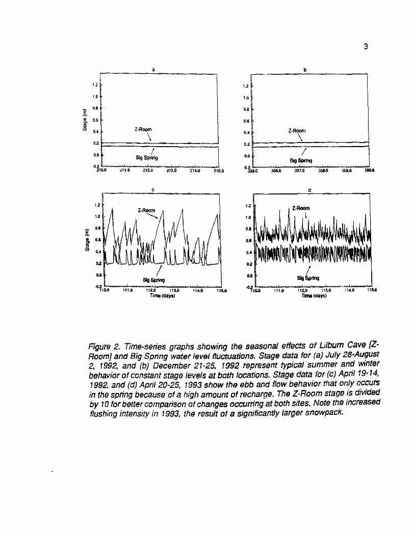
seasonal periodicity (Figure 2), occurring only during the spring snowmelt or in
periods of high recharge to the karst system. This flow phenomena is relatively
uncommon, found only in a few dozen springs throughout the United States
(Meinzer, 1942; Bridge, 1924).
Because of the unique nature of the ebb and flow behavior, few detailed
studies of this type of flow mechanism exist. This research may provide an
analogy for other studies of ebb and flow systems in karst regions, and will also
benefit the National Park Service at Kings Canyon National Park by supplying
an interpretation of the karst system in Redwood Canyon.
In the summer of 1969, members of the Lilburn Cave Research Group
constructed a broad-crested weir at Big Spring to establish a pool for a stage
datum. The weir is made of concrete and is approximately 1.1 m wide, 1.2 m
1

/
To Fresno
/ /
_,,.-, (90km)
N
/ /
/
NEVADA
SiUDY AREA
/ /..-.' oL:as Vegas
' CAI.IFORNIA
119°57'30"
2
Figure 1. Map of study area showing location of Big Spring. Dashed section of Redwood Creek shows its traverse through Lilburn Cave.
3
a b
1.2 1.2
1.0 1.0
g o.a 0.8
~ 0.6
~ ••• o.• Z·Room Z·Aoorn
\ o.• \
0.2 0.2
o.o Big Sing 0.0 I
Big S(lting
""·~10.0 211.0 212..Q 213.0 214.0 215.0 ""·~.o ,.._, 357.0 l$8.0 35i.O 310.0
c
1.2 12 Z·Aoom 1.0 1.0
E 0.1 ...
~ ••• 0.8 .. !11
"' ~· ••• 0.2
~· ••• BIQ~ .. ~ ... 111.0 112.0 1f3..0 114.0 115.0
..~ 110.0 111.0 ....
Timo(daysl
Figure 2. Time-series graphs showing the seasonal effects of Lilburn Cave [ZRoom] and Big Spring water level fluctuations. Stage data for (a) July 28-August 2, 1992, and (b) December 21-25, 1992 represent typical summer and winter behavior of constant stage levels at both locations. Stage data for (c) April 19-14, 1992, and (d) April 20-25, 1993 show the ebb and flow behavior that only occurs in the spring because of a high amount of recharge. The Z-Room stage is divided by 10 for better comparison of changes occurring at both sites. Note the increased flushing intensity in 1993, the result of a significantly larger snowpack.

4
high, and 0.3 m deep. A Stevens Model F strip chart recording hydrograph was
installed at the pool datum to continuously measure stage levels (related to
discharge) at Big Spring. Data were continuously recorded through spring of
1975, followed by several years of sporadic data collection due to recorder
problems. After spring of 1985, no data were collected due to lack of upkeep on
the Stevens recorder.
In the fall of 1988, the recording system at Big Spring was upgraded to a
digital datalogger, which in turn receives signals from a pressure transducer to
measure changes in stage, two temperature probes to monitor both water and
air temperature fluctuations, and an electrical conductivity (EC) probe to
measure changes in total dissolved solids (TDS). The data are recorded on a
standard cassette tape and translated into a readable format using a C20
cassette interiace. Data collection was sporadic through spring of 1989 owing to
instrumentation problems. Data collection has been fairly continuous since
summer of 1989. Figure 3 is a photograph of Big Spring showing the broad
crested weir and the datum pool with the location of the datalogger.
Objectives
The goal of this research is to gain a better understanding of the
hydrologic relationship between Lilburn Cave and Big Spring by testing the
current ebb and flow theories using various methods of time series analysis.
Because of the unique nature of the periodic ebb and flow discharge cycles

Figure 3. View of Big Spring with the datum pool at the center of the picture. Datalogger is located on top of the corrugated stack, and the water cascades over the weir in the foreground.

6
associated with this system, few detailed studies of this type of flow mechanism
exist. However, most of the theories offered to explain this mechanism are
based solely on observations made at the spring. The situation at Big Spring is
therefore unique, since access into Lilburn Cave allows for the system input to
also be studied. The current theory regarding the mechanism for ebb and flow
behavior at Big Spring is that of a sediment plug stochastically reacting in the
lowest sump of the conduit system, proposed by Sara (1977). This theory,
along with other proposed models on ebb and flow springs, will be tested to
determine the most probable mechanism for the cyclic behavior at Big Spring.
Geology
The tectonic events that resulted in the Sierra-Nevada mountain range,
summarized in Table 1, followed a long period of marine deposition during the
Paleozoic time and were initiated by the subduction of the eastward-moving
Pacific plate beneath the westward-moving North American plate (Harris and
Tuttle, 1984). The granite core of the Sierras formed during the Mesozoic from
about 210 to 80 million years ago, with uplift beginning approximately 150
million years ago during the Nevadan orogeny. From 80 to 30 million years ago
there was a pause in tectonic activity resulting only in erosion, which exposed
roof pendants of metamorphosed marine sedimentary rock.
A volcanic episode extending from 30 million years ago to the present
began in the middle of the Oligocene and placed approximately 1 km thick of

7
Table 1. Generalized geologic column for Sequoia and Kings Canyon National Parks. From Harris and Tuttle (1984).
TlmoUnils Rod<Unia Geobgie Events Era Period Epoeh
a - glaciol, and ..... Strumomo100. neogll<illa.:tMty, lanGalides, u H- wllllino~
..... _ • I
Earthqua"-. fauling, continuing upWt .
• r
c " Til.- 911<i1101lWIIIh Al.._t thr. ml4or gtlciations indudinq slob-• • Ploiolo<ono of v.no...avee: waAr~nc:M Olllgoo; ,,...,.. Qll<ill..,.., IIValoncho • r ~ -~--.lliacial 0 y ~ F...n.g, ...,od ll!>illt.
' 0
i N --olgllleiation c • Pliocene Southoms..,.-......,, __ ,
0 c~. intense eros10n
Q iloginning of faulting end uplilt T • W-ord ulting of--bloof< • •
r • Mioeo,.. I I
• p r • Oli!jocono e.-y I
• 0 Eocone g
• PauM 11 tectonic activity n Paloocene
Probllble ~inn1n9 ol cave deYelopmnm •
M c .......... Quartz cUoril•. qu.tz Empilcemltm a plutons in c:c~•· batnol!th • rmnzonlM, granodiort-. ~iam of country roc:K
' NeYtldan Of'09llf1'f 0 J ....... z Linestonet. ihal111, Marine tedimantatton and island arc vok:an1sm 0 Wld&t(.lfiM, ll'llert»edded SIA;)duetk>n and plale convergence i TMI&ic with vok:ana. c
p
• I
• (not '"""*od in patloa) Long aa:umullt"" a sodimonto 0
in PafeozO«:: sea
' 0
i
c

lava and mud flows in the northern Sierras (Hill, 1975). About 20 million years
ago, both the northern and southern portion of the Sierras were uplifted and
tilted westward. Thus, the mountain range is asymmetrical; it has steep slopes
on the fault-bounded eastern margin and a gentler regional slope to the west.
Along the eastern foot of the range is the Sierra-Nevada normal fault system,
trending north-northwest, with an estimated vertical movement of at least 4600
m (Harris and Tuttle, 1984).
8
In the western section of what is now the boundary of both Sequoia and
Kings Canyon National Parks, marble contained in the roof pendants has been
partially dissolved by groundwater to form underground caverns such as Crystal
Cave, Palmer Cave, and Lilburn Cave. The metamorphism that changed
limestone to marble destroyed any fossils that may have existed. Fossils found
in Mineral King approximately 25 km southeast, however, have been dated as
Upper Triassic (Ross, 1958).
Redwood Canyon
The Redwood Canyon area of Kings Canyon National Park is bordered
on the west by Redwood Mountain (Figure 4), a metamorphic roof pendant
trending to the northwest, that is surrounded by igneous rocks. The roof
pendant is a schist composed of 25 percent potassium feldspar, 25 percent
biotite, 35 percent quartz and the remaining 15 percent muscovite, epidote,
and accessory minerals (Ross, 1958). Ross conjectured the parent rocks to be

' . . . r1-' : "'"'¥- -:XI ""!-" . .... ry-. ·.01.\l
..... o-·. ,...,_ : . . /'"'- ~ .z. . . . """ . .,:: 0 . . ,_ ,..,....._ 0
·n-·. o- ..
. ·;__:_. Quartzite, :/"'\..-~ · · Schist ~ .·. · "' "-· ..
/"'o-'.
-9- ,,
II If
~ 1\
"1\ ~ ..
-;-' ~
" 1/ ~
,, -7 'l
1\ !l ,, Big
- ~ Granodiorite 4" ::::. ,, ~
// ,, \\ tr \\ ~ 1/ II ., \\ /(
' ( ' \ / I
/
Granite I ' \ / ' '-\j '"' ( \. ' I \ ' ( I ' lj \. ' I ' " \ I
1' I I ,I 'I '
' I ' '- I
' I' I 't" '-
( " ( I
' co /
-· ...... \ ,.. ~ tO " I ...... I'
I co I ' / 0 I I ,
,'1 - \ ... a.. -" ......::. I ..
\. ( ,"- /C) / .. -· ' 'I a..
( \. tO ,_
Ctl '-.I
' ,; -\
/ I \ I I' ' ,_ I' \.
\ I" '-, I I' "
'- I
' i I "' ' N /
~ \ 0 600 ...... METERS .. \
Figure 4: Geologic map of Redwood Canyon showing the location of the marble lens within the roof pendant. Modified from Sara (1977).
9

shales, argillaceous siltstones, and fine-grained sandstones in an intermixed
sequence.
Redwood Canyon is bordered on the east by Big Baldy Ridge (Figure 4),
a granitic pluton. The pluton is exposed over an area of approximately 1.2 km2
and shows jointing characteristics of exfoliated domes (Ross, 1958). Ross
described Big Baldy granite as medium-grained composing of 50 percent
potassium feldspar, 25 percent oligoclase, and 25 percent quartz, with trace
amounts of biotite and hornblende.
The floor of Redwood Canyon consists of a marble lens trending
northwest througt1 ttw metamorphic roof pendant. Figure 4 shows the location
of this lens in relation to the surrounding geology and Lilburn Cave, as mapped
by Sara (1977). The grey and white banded marble ranges from dolomite to
calcite in composition and is dipping nearly vertical (Sara, 1977). There are
several areas of sinkholes, mostly in the northern portion of the karst area.
Sinkhole sizes vary from shallow, 2 to 3 m diameter sinkholes to as large as
200 m wide dolines (Cave Research Foundation Personnel Manual, internal
publication).
Relief of the Redwood Canyon area is pronounced, ranging from an
elevation of 1350 m where Redwood Creek enters the north fork of the Kaweah
River, to 2500 m on Big Baldy Ridge. The walls of the canyon rise 915 m in 2.4
km (38% slope) on the east to Big Baldy Ridge, and 365 m in 2.4 km (15%
slope) to Redwood Mountain to the west.

11
Lilburn Cave
Lilburn Cave is located at 36.6N and 118.9W, which is near the center of
Redwood Canyon at section 35, T.14S, R.28E in the USGS Giant Forest
Quadrangle. The entrance to the cave is at the bottom of a large sinkhole about
15 m wide and 6 m deep, at an elevation of approximately 1580 m (Halliday,
1962). The cave entrance is accessible via an approximate 8 km foot trail
beginning from the Redwood Canyon saddle at the north end of the canyon.
Since 1968, over 21.7 km of cave passages have been mapped (Cave
Research Foundation Annual Report, 1992) striking mainly N1 OW that
encompasses an area over 2560 m long by 460 m wide (approximately 1 km2).
The marble bedding within Lilburn Cave is nearly vertical (Halliday, 1962). Its
upper regions consist of a spongework dissolution pattern in the marble forming
a complicated maze of passages covered everywhere with mud. At greater
depths, the walls are clean of mud, displaying white and blue-black banded
marble. Draperies, cave bacon, and stalactites have formed in only a few areas.
History of Lilburn Cave
There are different versions regarding the discovery of Lilburn Cave, the
most probable described by the Cave Research Foundation Personnel Manual
(undated). In the early 1900's, a prospector found the cave entrance and
ventured in. After penetrating a short distance, he was supposedly startled by
loud reverberations coming from within the cave and quickly left. George

Lilburn, formerly of Indiana, filed a mining claim near the entrance of the cave
on August 5, 1931, but did not rediscover Lilburn Cave (formerly known as
Redwood Canyon Crystal Cavern) until July 3, 1940. Several meters of
landslide debris had to be excavated before he could gain entrance.
12
Lilburn hoped to commercially develop the cave in 1941 and later sell it
to the National Park Service (NPS). This venture was in vain because of the
ruggedness of the cave and the general lack of speleothems. By 1941 the NPS
took control of the cave and decided not to commercialize it due to the nearby,
recently opened Crystal Cave.
Lilburn based his operations out of the former cabin that once stood in
the location of the present Cave Research Foundation's field station. This cabin
is said to have been built by a miner named Robinson sometime between 1900
and 1930, possibly in conjunction with development of the nearby Redwood
Canyon tungsten mine. The mine has been inactive since the 1970's because
of a landslide that covered the workings.
Hydrology
The drainage area contributing to the total discharge at Big Spring is
approximately 25.3 km2• The irregular-shaped watershed is approximately 4 km
east to west and 9 km north to south at its widest points, and consists of slopes
of granitic and metamorphic rocks, colluvial material from Big Baldy Ridge, and
a well integrated surface drainage through the marble roof pendant. Redwood

13
Creek, which is the main drainage of Redwood Canyon, and many small
tributaries sink at or near the contact of the marble and granite and flow
through the subsurface drainage system, forming Lilburn Cave, before resurging
at Big Spring.
A perennial stream flows through Lilburn Cave and represents the
underground flow of Redwood Creek (Figure 5). East and West Streams,
flowing within the cave from channelled surface drainage, and surface streams
of Pebble Pile and Mays Creeks, contribute to the complex hydrology of the
cave system.
Pebble Pile Creek sinkhole collapsed in the summer of 1988 adding
sediment approximately 5 m in thickness into Lilburn Cave just upstream of the
Z-Room (Tinsley, 1992, personal communication) which could have affected the
flow behavior at Big Spring. In 1984, prior to the sinkhole collapse, a qualitative
dye trace was performed which confirmed a connection between Pebble Pile
Creek and Big Spring, but detectors were incorrectly positioned within Lilburn
Cave to determine where Pebble Pile joined Redwood Creek (Cave Research
Foundation Annual Report, 1984). After the sinkhole collapse, the contribution
from Pebble Pile Creek into Lilburn Cave was no longer evident. In May 1993,
Pebble Pile Creek was observed filling the sinkhole, and water was observed
sinking into at least one 6 to 8 em hole. The passageway between River Pit and
the Z-Room within the cave was very wet with pervasive, constant dripping from
the ceiling. This could be the contribution from the Pebble Pile Creek sinkhole.

TOP OF KARST OF: REDWOOD CANYON"":
i N
0 1
KM
~ RESURGENCE f;m AREA OF LILBURN liiSli CAVE
/ {
\
'
14
Figure 5. Hydrologic map of Redwood Canyon showing known surface streams that join Redwood Creek and flow into Lilbum Cave.
15
Big Spring is the resurgence of Redwood Creek after its subterranean
traverse through Lilburn Cave. The last accessible point without diving in Lilburn
Cave is the South Seas room, which is located approximately 700 m north of
Big Spring and about 10 m higher (Moore and Sullivan, 1978). Analysis of
previous data from Big Spring indicates that ebb and flow behavior occur during
spring snowmelt periods with measured flow discharge fluctuating between 0.4
m3/s and 5.1 m3/s within several minutes (Sara, 1977).
Big Spring and Lilburn Cave SCUBA diving
In 1974, divers using SCUBA penetrated Big Spring and observed a
passage 1.5 to 2 m high and 3 to 3.5 m wide (averaging a 2.4 m diameter
circular conduit) extending down a sandy, silty slope varying from 45 degrees to
nearly vertical (Sara, 1977). The divers penetrated approximately 150 m into
the spring, reaching a depth of 53.5 m before turning back (this is about the
limit for fresh water, high altitude SCUBA diving). Information yielded from this
dive indicated:
(1) because no other passages were found, this is postulated to be the
main source of water to the spring.
(2) sand and silt are present in great quantities in both the spring
passage and in the north entrance of the main cave system,
(3) if a siphon or second conduit is present, it must join the main
resurgence conduit lower than 53.5 m.

16
The most recent dive into Big Spring occurred in September 1991. A
partial constriction of sand was observed approximately 22 m into the passage
(Cave Research Foundation, unpublished). No evidence of a sand plug had
been observed on any previous dives, but it is possible that one could have
been present below the allowable diving depth.
A dive into the South Seas room in Lilburn Cave occurred in October
1991. This dive revealed a large, silty room approximately 15 to 30 m across
and 30 m deep with possibly three major leads. Exploration was limited
because of the allowable diving depth for high altitude SCUBA diving,
preventing further exploration.
Vegetation and Climate
The vegetation of Redwood Canyon consists of large groves of giant
Sequoias at elevations above 1700 m, with a transition forest of sugar pine,
cedar, and bush growth of manzanita, pear clover, and wild cherry below 1600
m (White and Pusateri, 1949). John Muir considered Redwood Canyon as a
significant giant Sequoia areas and was quoted in White and Pusateri (1949):
"Here the Sequoias attain full possession of the forest for several miles,
covering the hills ... in magnificent order."
Climatological records obtained from the Grant Grove ranger station
indicate that precipitation in Redwood Canyon since 1942 has averaged 1 08 em
of rainfall plus 468 em of snowfall each year. The precipitation falls primarily

17
from October through March, with average temperatures ranging from 3 to 18°C
in the daylight hours to -0.5 to 7°C at night. The summer months are typically
dry with average maximum temperatures ranging from 11 to 25°C and minimum
being from 0 to 12°C.
Current theories on ebb and flow springs
Ebb and flow behavior is historically explained through the presence of
intermittent natural siphons within the rock matrix behind the spring (Meinzer,
1942; Bridge, 1924; Sweeting, 1973; Bonacci, 1987; Jennings, 1987). In a true
siphon (Figure 6a), when the level behind the siphon builds up to B, water
begins flowing over the crest at C and the siphon is activated dropping the
water level rapidly to A. At A, air is allowed to enter the main flow conduit,
breaking the siphoning action. This configuration results in the spring drying up
in between flows and very consistent flow variations, with the spring always
rising and dropping to the same maximum and minimum stage levels.
Sweeting (1973) and Jennings (1987), however, have found that most
ebb and flow springs are actually reciprocating springs (Figure 6b), where,
unlike a siphon, flow continues in the ebb cycle at varying discharges.
Reciprocating springs are explained by the filling of an inactive passage during
high recharge periods, substantially increasing flow at the spring. An example of
a reciprocating spring is Ebbing and Flowing Well in Yorkshire, England, where
Stevens (1964) quotes an observation written by John Swainson on April 7,

18
Figure 6. Cu"ent models regarding ebb and flow springs: (a) natural siphon present within the rock matrix [Meinzer, 1942]. When the water level behind the siphon C builds up to B, the siphon is activated and the water level drops rapidly back to A; (b) reciprocating spring {Sweeting, 1973; Jennings, 1987]. Flow occurs through conduit B to spring A, and when the water level in the cave rises it activates conduit C increasing the discharge at A; (c) sediment plug [Sara, 1977]. Water transported through plug as porous media flow until hydrostatic head is sufficient to breach plug out through the spring.

19
1796 describing the phenomena: "Settled 11 inches in about four minutes; it
flowed to the same height in two minutes. Next time it did not go so low by two
inches. When at low ebb it begins to rise immediately. There seemed no
interval between its low ebb and rising, nor betwixt its being full and beginning
to ebb again."
Sara (1977) suggested that ebb and flow cycles at Big Spring were the
result of a sediment plug (Figure 6c), in which an ebb cycle is created through
blockage at the lowest sump of the system by sediment deposition. When the
constriction is breached because of an increase in hydraulic pressure from
additional recharge, the flow cycle resumes. A sediment plug would not
completely block off flow as an air trap in a siphon would. The volume of water
allowed to percolate through this sediment plug is controlled by the hydraulic
conductivity and cross-sectional area of the plug. This mechanism suggests a
large, coarse-grained sediment source within the flow system. Varying sizes of
the transported sediments result in changing permeabilities of the plug. This
may account for the irregular discharge volumes observed at Big Spring.
The data collected from Big Spring will be applied to the above
mentioned models to determine the most probable geometric karst network
operating within this system.

Physical Methods
CHAPTER 2
METHODOLOGY
Data/agger installation and programming
20
In the fall of 1988, a Campbell 21 X digital datalogger was installed at Big
Spring to measure changes in stage (Druck pressure transducer, type PDCR
1 0/D, accurate to ±0.1 %), water and air temperature (Campbell Model 107
temperature probes, accurate to ±0.1'C), and electrical conductivity (YSI Model
3310 EC probe, accurate to ±1 %). In November 1991, a Campbell CRt 0 digital
datalogger was installed within Lilburn Cave. The installation of the cave
datalogger is shown in Figure 7. The CR1 0 is a newer model of the 21 X
datalogger, which stores the data internally allowing for data to be transferred
into a portable personal computer or memory module instead of on a cassette
tape. A similar pressure transducer, and water temperature and EC probes
currently in place at Big Spring were installed in the Z-Room (Flush Room) of
the cave (Figure 8), where the water level displays the cyclic fluctuations that
correspond to the flow variations at the spring. A pressure transducer and water
temperature probe were also placed at the River Pit (Figure 8), approximately
250 m upstream from the Z-Room. The datalogger was placed at the
approximate location shown in Figure 8, with about 140 m of cable extending
down to both the Z-Room and River Pit. The datalogger was placed here
because it is a central location for both sites, and is potentially out of reach

Figure 7. Hydrologist Brad Lyles programming the Z-Room and River Pit datalogger inside Lilburn Cave. Note the PVC manifold (upper left) containing the datafogger and transmission lines routing to the various sensors. Batteries are sealed in a water-proof ammo box below keypad.

0 50 100
VERTICAl AN> HORIZONTAL SCALE {METERS)
Figure 8. Schematic of a cross-section of Lilburn Cave showing the location of the datafogger in reference to the River Pit, Z-Room and Big Spring.
Big Spring .. 100 m

23
from high water levels. The datalogger was sealed in a water-tight PVC casing
with the batteries sealed in a metal box. Both were attached to a large boulder
in the rare event that the water level will reach this position.
Both the Big Spring and Lilburn Cave dataloggers were set with a scan
rate of 15 seconds. The trigger levels for data collection and storage were
changed on several occasions, and these are tabulated in Table 2. An example
of the datalogger data can be found in Appendix A.
Stream gaging
To quantify the discharges from Big Spring, a weir was installed in 1969
by members of the Lilburn Cave Research Group so as to establish a pool
datum to measure stage height. According to Sara (1977), V-notch weirs initially
installed were washed away during the spring flow periods; therefore, a
concrete broad-crested weir was constructed to resist the maximum flow.
A Gurley No. 625 Pygmy current meter was used to gage Big Spring
approximately 10 m downstream of the weir in order to relate discharge to
stage height in the datum pool. The gaging site was chosen because it had a
relatively smooth stream bed with minimal eddy currents. The stream was
gaged during three different flow periods, with a single current meter reading
taken at 60 percent of the depth at each chosen mark. The stream was
approximately 1.8 m wide at the gaging site and was divided into 7-12 equally
spaced sections. The number of Pygmy meter revolutions at each mark for one

Table 2. Instrumentation and programming changes made to the dataloggers at Big Spring and within Lilburn Cave.
Date
09/01188
11/02191
03/08/92
04/12/92
05124192
11101/92
03113193
localion Reasons IOi Changes
Big Spring Removed Stevens recorder and instaUed digital datalogger lor better accuracy and ease of data analysis.
Z·Room Installed datalogger lo monitor Input into Big Spring.
River Pit
Big Spring
Z-Room
River Pit Z-Room
River Pit
Z·Aoom
Big Spring
Big Spring
lnstaJJed dalaJogger 1o monUor input into the Z-Aoom.
ln&talled Manning &ediment sampler 1o monitor sediment movement out of spring. Reprogrammed datalogger tor more detaHed anayrsis.
Added trigger level lor stage changes. EC data Huctuating too much and overloading datalogger memory.
Stage trigger changes not very si nllicanl. Observed pressure transducer dislodged changing the stage datum at an unknown time and amount. Reprogrammed to collect high lrequency stage da1a for detailed hydrograph analysis.
Manning automatic sediment aampJer found knocked over due lo high water event.
Changes Performed
Record data every hoLJr and when trigger levels exceeded~
stage: f 0.03 m water temp: ± 0.1 degree C EC:± 10%
Record sfage. water temp and EC every hour.
Record stage and water temp every h()ur.
Collect 250 ml water sample every 1 o minules white stage > 0.3 m. New trigger levels:
stage:± 0.15 m water temp: ± 0.1 degree C EC:± 10%
stage: ± 0.03 m Removed EC trigger.
Removed stage trigger.
Aller the first flush of 1993, record 2000 stage records at one minute inteJVals rollowed by 5000 records of normal data collection. Disconnect Manning sampler.

minute were recorded, and the average velocities (m/s) were calculated by:
v = 0.30 * (revolutions/second).
The velocity (v) multiplied by the area (A) of each section will result in the
discharge (0) in each subdivision from the continuity equation:
( 1 )
Q = Av (2)
The sum of the discharges of each section is equal to the total flow of the
spring (Table B1 ).
25
A few difficulties were encountered while stream gaging that probably
added error into the calculated discharge values. First, the irregularity of the
stream channel made calculating the stream area difficult. Second, the depth of
water was only measured accurately to 0.5 inches (1.27 em). which may have
resulted in an error in computing the channel area. Problems were encountered
on May 2, 1993 when the flow at Big Spring was very high. The high flow of the
spring made it difficult to count the number of revolutions of the pygmy meter.
Duplicate readings could not be obtained because the spring was flushing and
the gaging had to be completed quickly with the least amount of stage level
changes.
Flow in the River Pit was also gaged on two events using the same
Pygmy current meter to obtain information on water entering the Z-Room. The
River Pit measured 1.3 to 1.5 m across at the gaging site. with flow determined
with the above procedure (Table B2).

26
Sediment Sampling
A Manning portable discrete sediment sampler (Model S-4400) was
installed at Big Spring in November 1991, with the intake hose placed in the
datum pool. The sediment sampler is programmed by the datalogger to collect
a 250-ml water sample when the stage at the spring is greater than 0.3 m,
indicating a period of flushing. The sampler will continue to collect a sample
every 1 0 minutes until the stage drops below 0.3 m. Transient flow of sediment
and a resulting blockage of the underground flow path may be an important
control on the hydrologic system. Analysis of any sediments that may be
collected with the water samples may suggest the influence of previously de
posited sediments that are being flushed out of the spring. This may aid in
understanding the hydraulics of this cave-spring system.
Sediment samples were collected from the stream beds at Redwood
Creek and at Big Spring at varying distances downstream to determine a
particle size distribution and the dominant mineralogy. Two sets of samples
were sieved for particle size analysis using a rototap for 15 minutes each. The
amount o1 sediment that remained in each sieve was weighed to determine the
percent distribution of each size, then classified using the Wentworth sediment
scale (1922).
Water chemistry
Water samples were collected at Redwood Creek both before it enters

27
the karst and when it resurges again at Big Spring to observe chemical
changes throughout the karst system. The samples were analyzed for gross
chemistry by following United States Environmental Protection Agency (USEPA)
standard procedures at the Desert Research Institute Water Chemistry Lab in
Reno, Nevada. The concentrations of the species present were further analyzed
using WATEODR, a geochemical computer model that calculates mineral
saturations. Field titrations were performed on two of these sampling events at
both Redwood Creek and Big Spring using a Hach digital titrator, Model
16900~01 (accuracy±!%), to determine the field alkalinity of the input and
output waters.
Precipitation
Daily precipitation and climatological data were obtained from the Grant
Grove Ranger Station for 1990 through the present, and historical yearly data
prior to 1990 was also made available. Grant Grove is approximately 3 km
north of the drainage basin and is the nearest location where precipitation is
monitored on a daily basis. Daily total precipitation was determined to be the
depletion in the snowpack multiplied by the average water content and added to
the rainfall. Although this does not result in the actual recharge to the Lilburn
Cave system, it gives the relative magnitude of changes in recharge.
28
Bench-scale model
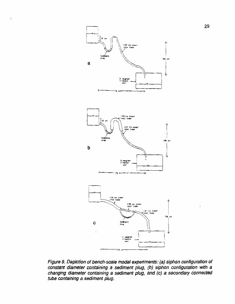
A laboratory bench-scale model was developed to simulate the ebb and
flow discharge cycles observed at Big Spring. The first experiment (A), shown
diagrammatically in Figure sa, involved a siphon of a constant size clear vinyl
tube (1.27 em inner diameter). The upper reservoir was a 1 0-~ bucket with a
1.27 em ball valve installed 3 em from the bottom to control the flow. The lower
reservoir was a 40.5 em long, 21.5 em wide, and 27.5 em high acrylic plastic
container with an 11 o V-notch weir installed beginning approximately 3 em from
the bottom. Water was added to the upper reservoir at a constant rate of
recharge to observe the hydrodynamics involved in a siphon configuration.
The second experiment (B) utilized the same siphon configuration but
added an 8 em plug of sediment in the lowest sump, with sediment sizes
ranging from 0.3 mm to 15 mm. A constant rate of recharge was added to the
upper reservoir to determine the effect of a sediment plug on ebb and flow
behavior.
The third configuration (Experiment C) involved a siphon configuration
and sediment plug, with a larger tube (1.9 em inner diameter) attached above
the sump (Figure 9b). When the hydraulic gradient is sufficient to breach the
plug, the sediment will enter the larger cross-sectional area which has a lower
velocity. This experiment simulated a conduit of varying sizes possibly affecting
the flow.
The final experiment (D) simulated a secondary conduit, pluggei with
29
, ....... J r v-• .. ne~ ... t-----"----1
b
---176 e, __ _::::::::;--_J
Figure 9. Depiction of bench-scale model experiments: (a) siphon configuration of constant diameter containing a sediment plug, (b) siphon configuration with a changing diameter containing a sediment plug, and (c) a secondary connected tube containing a sediment plug.

sediment, that is activated with sufficient hydraulic gradient (Figure 9c). A 1.9
em inner diameter tube was split into two 0.9 em inner diameter tubes so that
the input capacitance was greater than the capacity of the tubes that split off.
30
All four of these experiments were tested for the duration of several flush
events, and were digitally recorded using a CR1 0 Campbell datalogger and two
Geokon pressure transducers, programmed to record stage in both reservoirs
every 15 seconds.
Analytical Methods
The digital datalogger continuous data set of the Lilburn Cave-Big Spring
system was analyzed using various methods of time series analysis.
Hydrograph analysis was performed on the Big Spring flow data to determine
information about the karst aquifer system. The spectral analysis analytical
methods of power spectra, transfer and kernel functions were used to compare
Lilburn Cave (input) and Big Spring (output), which provided information on the
cave-spring flow dynamics and development of a conceptual model of the
system.
Hydrograph analysis
A spring hydrograph is a means of graphically representing the variation
of spring discharge with time. The shape of the hydrograph is a function of the
underlying karst geometry and can thus be examined to reveal information on

31
the groundwater movement within the aquifer.
Types of carbonate aquifers
Aquifer tests and recharge-runoff analyses are typical methods for
evaluation of aquifer properties in most kinds of rock. Most of these techniques
in their standard form are not effective tor evaluation of mature karst aquifers
because of complexity within the matrix. Caves can be mapped, which gives a
partial picture of the conduit system, but does not provide much information
regarding the smaller openings in the aquifer which may be the most important
in terms of total available aquifer porosity.
Wilcock (1968) and Ashton (1966) treated the carbonate aquifer as a
black box with an input (sink) and an output (resurgence) in order to bypass
this problem. This approach is known as flood-pulse analysis, in which the input
pulse is the flood wave which enters a cave when precipitation or snowmelt
occurs. The black box is a model of the internal geometry of the cave system,
which may be derived from field observations of the measurable inputs and
outputs.
Most springs are known to have fluctuating discharge rates usually
ascribed to variations in frequency and intensity of local precipitation. A spring
hydrograph is a means of graphically representing these fluctuations in
discharge with time, which vary in magnitude and shape. The shape of the
outflow hydrograph recorded at a spring is a unique reflection of the response

32
of the aquifer to recharge events and changes in bulk sediment position or
volume (Ford, 1989). Consequently, the analysis of the hydrograph shape may
provide information on aquifer properties, such as permeability, storage capacity
and hydraulic geometry.
Karst aquifers differ from aquifers within other rock types mainly because
their permeability increases with time as carbonate rock is removed by
dissolution (White, 1977). Two main flow regimes were defined by White (1988)
to categorize karst aquifers: conduit flow and diffuse flow. Conduit flow aquifers
consist of flow through a network of conduits (pipes) with a passage size
ranging from a few centimeters to tens of meters (Gaither, 1977). Flows in
these aquifers are largely due to gravity governed mainly by the hydrostatic
head, the hydraulic and geometric characteristics of the conduit, and the
volume of recharge to the system. Drainage patterns have been found by White
(1988) to be underground extensions of surface streams rather than as
groundwater, with discharge typically occurring through springs. They carry a
sediment load both as suspended load and as bedload, a feature not found in
diffuse flow systems (White, 1969). Springs and cave streams in conduit flow
systems respond quickly to recharge, resulting in a ratio of 10:1 to 1000:1
(Quinlin, 1990) between maximum and base flow discharge. The discharge
responds rapidly to recharge with a flow that is generally turbulent.
Diffuse flow aquifers consist of flow occurring along bedding planes,
faults, joints or fractures (White, 1988). If a conduit system is present, it will be

33
very poorly integrated. White (1969) found that diffuse flow typically occurs in
less soluble rocks such as extremely shaley limestones or crystalline dolomites.
These aquifers are not as developed as conduit systems, resulting in less
sudden recharge responses and possibly laminar flow at the spring. Quinlin's
(1990) research determined the ratio between maximum to base flow discharge
for diffuse flow aquifers to be 4:1 or less. Most karst aquifers have been found
to contain some amount of both conduit and diffuse flow regimes.
The pore space geometry which develops in a karst aquifer can be
thought of as an interconnected system of pipes. Some karstic passages are
only active when the recharge is so intense that the aquifer fills to higher than
normal levels. Because of the intricate arrangement of the karst conduits,
various unusual hydraulic phenomena such as the development of a natural
siphon can occur.
Basic hydrograph components
A typical hydrograph recession limb of a transient recharge event is
shown in Figure 10 and can be divided into four basic parts (White and White,
1974).
(1) Rising limb: This portion of the hydrograph begins at the first increase
in spring discharge and continues to the first inflection point. The rising limb
represents the increase in discharge caused by an increase in storage of the
reservoir. Its shape, usually slightly convex upward, and slope are influenced by

RISING LIMB
iCRESTi I I I I I I I I I
Oo --
RECESSION LIMB
Time (t)
BASE FLOW
Figure 10. Typical hydrograph of a discharge event for a karst spring. OM = peak discharge, 08 = base flow discharge, 00 = start of recession discharge, t, =recovery time. Modified from White and White (1974).
the travel time of water from different areas of the basin.
(2) Crest: The crest segment of the hydrograph is located between the
upper inflection points of the rising and falling limbs. The crest contains the
34
peak instantaneous discharge for the precipitation event. When the hydrograph
is at its peak, storage in the karst system is at its maximum. Irregular basin
shape and oscillating rainfall intensity can result in two or more peaks from a
single transient event (Linsley, et. al. 1949).

35
(3) Recession limb: The recession limb begins at the first point of
inflection on the falling limb and continues until the flow levels off to baseflow.
The time for the recession to occur is the aquifer response time, t,, which
represents the removal of water from storage after its recharge. Its slope,
therefore, may be considered as the natural rate of aquifer depletion. Fast
aquifer response times can be an indication of a conduit flow system with little
aquifer storage, whereas a diffuse flow system will have a slower response,
indicating a larger aquifer storage volume that is being slowly drained. Gaither
(1977) states that the recession limb is dependent only on the physical features
of the flow path and system and is independent of time variations in rainfall.
(4) Base flow: The base flow portion of the hydrograph represents the
sustained flow of the aquifer system. The recession limb will exponentially
decay to base flow.
Hydrograph analysis techniques
As stated earlier, analysis of the recession curve can provide information
regarding the characteristics of the karst aquifer. This curve is generally uniform
since the characteristics of the aquifer should stay constant between each flow
cycle.
In 1905, Maillet derived the general retardation curve equation which
expressed the discharge rate of a spring:
(3)

36
where 0 1 (m3/s) represents the yield in the time interval (t-10) as a function of the
yield 0 0 (m3/s) at time 10 taken at the start of the recession (zero recharge) of
the aquifer. The depletion coefficient k (1/time), is a measure of the aquifer
response to a release of storage. When the recession curve is plotted on a log
linear scale, k is the slope of the curve, which is negative as a result of aquifer
depletion. This term is dependent primarily on the physical features of the
conduit flow system, such as conduit size, and the geometry, distribution and
relative position of the karst conduit system with respect to the water table
(Bonacci, 1993; Gaither, 1977). Qualitatively, k expresses the relationship
between aquifer geometry and hydrology. High values of k (steep slopes) are a
result of fast-response aquifers related to conduit flow. The rate of discharge
will be high, which may indicate a high hydraulic gradient, a high transmissivity
and small available porosity. Low values of k (gentler slopes) indicate a slower
response due to the effects of a diffuse-flow aquifer, indicating a low hydraulic
gradient, and a lower transmissivity with more available porosity. Figure 11
graphically shows these two responses. Mijatovic (1968) states that for aquifers
discharging through cracks and joints, k is on the order of 10-3; for discharge
through open fissures and smaller tubes, k is on the order of 10-2, and for
discharge through tubes and channels, k has a magnitude of 1 o-t.

Oo (fast)
slope = k(fast)
time (t)
37
Figure 11. Graphical representation between a high and low depletion coefficient, k. Conduit flow aquifers will have a high value of k, or a fast rate of depletion, compared to diffuse flow aquifers which will respond more slowly.
In the case of monotonic discharge (discharge through an aquifer
displaying only one type of flow regime), the recession curve plotted on a log-
linear scale will be a straight line. This type of aquifer geometry is rare in karst
regions (Mijatovic, 1968). Because of the anisotropy and geometrical
irregularities in karst aquifers, the recession displays a complex curve that
represents more than one flow regime, and consequently, more than one
depletion coefficient. Flow through karst is very dynamic and non-stationary but
by dividing the recession limb into segments, it can be regarded as quasi-linear
(Bonacci, 1993), allowing for valid analysis of the system. Figure 12 is an
example of a complex recession curve with four flow regimes. At the start of the
recession, discharge takes place through all collectors, or geometrical flow

6 Ol
Q
...__ '--- -...I I-- ...... --1 -..
I Ou = 0 03e k3(1J IOJ
I -----~---- I
I -r- --. -- - - - - -I : --,1 ----- ----.-1 1 I
I I I I I I I I I I I
lo
Time (t)
Figure 12. Example of a complex hydrograph recession curve showing the different flow regimes that can be found in a karst aquifer. Modified from Mijatovic (1968).

39
paths, within the aquifer. At this point the curve is steep (segment 1 on Figure
12) and represents the sum of all the yields, i.e., that of large channels, tubes
and caverns, smaller channels and tubes, open fissures, and the uniform yield
of narrow fissures and fractures.
This is followed by a less steep segment (segment 2 on Figure 12) which
represents the sum of three yields, the yield of the large channels and tubes
being negligible since they typically drain quickly. Segment 3 is less steep than
2 and represents the sum of two yields, that of open fissures and of smaller
fissures and fractures. The last segment of the recession curve (segment 4) is
almost horizontal and corresponds to uniform discharge through the small
fissures and fractures within the aquifer.
Spectral Analysis
Spectral analysis of a time series consists of partitioning the data into the
unique frequencies at which the system operates. The representative time
series is regarded as the sum of these frequencies. This method can provide
valuable insight into the physical processes within the system, and are used in
the prediction of future behavior. The spectral methods of power spectra,
transfer functions and kernel functions will be applied to interpretation of the
Lilburn Cave-Big Spring system.

40
Power Spectra
Spectral methods are an application of Fourier analysis and are suitable
for stochastic, or random, processes that are a function of time (Jenkins and
Watts, 1968; Blackman and Tukey, 1958). Fourier analysis is a method for
approximating a function by a sum of sine and cosine terms. This approximate
function is known as the spectral density (S(m))
.. s ( w ) = .E p jeir.~ j (4)
-oo
where m is the frequency, p1 is the autocorrelation of jth order (Kendall and
Stuart, 1976). The spectral density plotted against the frequency is the power
spectrum, shown in Figure 13:
a b
0
In P,
-IS l-..-...!-----0 10
f
Figure 13. Typical power spectra for (a) a periodic system, and (b) a nonlinear or chaotic system [Drazin, 1992].

41
The power spectra looks determines any dominant frequencies that the system
might be operating at, which indicates periodicity in the data set. A linear
system will display peaks of diminishing amplitude in the power spectrum at the
harmonic frequencies (periods) in which it operates, as shown in Figure 13a. In
a linear system, the input can be related to the output on a linear scale, and
indicates that the system is homogeneous and steady, with no variation in
conduit size, saturation, or hydraulic conductivity. Nonlinear and chaotic
systems, however, result in broad-banded spectra rather than isolated peaks
and contain high levels of noise (Drazin, 1992), such as in Figure 13b.
Nonlinear behavior is usually the result of a non-homogeneous, non-steady
system with variations and inconsistencies found in the above mentioned
parameters.
Transfer Function
The relationship between two spatially separated time series is known as
the transfer function (Sheriff, 1984; Brown, 1970), and is represented by:
(5)
where (Jl(ID) is the transfer function, 9m(t) is the output frequency at time t, and
f01(t) is the input frequency at time t (Arfken, 1985). This function represents the
ratio of output to input (in this case, spring to cave) on an amplitude versus

42
frequency graph because, when the input is multiplied by this ratio, it equals the
output. It indicates the degree of attenuation that may be occurring within the
system. If the transfer function is greater than 1.0 or continually rises with
increasing frequency, the output is more variable than the input. This may
indicate additional inputs to the system between the input and output resulting
in increased turbulence. In linear systems, the transfer function will either be a
straight line at or below 1.0 or decrease with increasing frequency due to
attenuation of the input turbulence within the system.
Kernel Function
The kernel function is defined as the inverse Fourier transform of the
transfer function. The kernel function measures the response of an aquifer to
changes at the input or output, and is represented by the convolution integral,
y(t) =J~ .. h(t-T )x(T ) dr ( 6 )
where y(t) is the output or spring discharge, x(t) is the input or recharge
through the Z-Room, h(t-t) is the kernel function, t represents time, and t is the
variable of integration (Dreiss, 1982). The kernel function represents the
response of the system to an instantaneous unit input (Driess, 1989), in this
case, a flushing event triggered in the Z-Room. The kernel function can help

43
determine if the system is linear or nonlinear. If a single kernel can be found
that, when integrated with the input correctly predicts the output, then the
system is linear. If the kernel function remains near zero after its initial drop, the
system is assumed to be linear with no other inputs or outputs. A negative
kernel function indicates other outputs may exist, and a positive kernel function
indicates the possibility of additional inputs to the system. The amount of
variation of the kernel function around zero supplies information regarding the
type of karst aquifer present within the system (Dreiss, 1989). The variance in
the kernel function will be large for aquifers where travel pathways are highly
interconnected, and smaller for more mature conduit-flow aquifers where large
quantities of water are transmitted rapidly.
Data interpolation
Although several variables were collected from the two dataloggers used
in this study, only stage is studied here because of its variations. The available
computer models require equally spaced data to perlorm fourier or spectral
analysis. Since data collection was triggered by both significant variable
changes and an hourly flag, equally spaced data were not obtained. MacDonald
(1989) suggested data interpolation to smooth the uneven data spacing. The
data interpolation method used in this research was kriging, which produces
estimates that have the smallest possible error in relation to other conventional
estimation procedures (Davis, 1986).

Physical Methods
CHAPTER 3
RESULTS
44
The results of the physical methods of stream gaging, sediment and
chemistry analysis, the effects of precipitation, and the time-series and bench·
scale model observations will be presented in this section.
Stream gaging
Big Spring was gaged on five separate occasions approximately 10 m
downstream of the weir using a Gurley No. 625 pygmy current meter to develop
a rating curve relating discharge to stage measured in the spring's datum pool.
From these data (Table B1), a discharge-stage rating curve was developed, as
shown in Figure 14. The equation of the curve as obtained by using a quadratic
regression analysis is:
y(stage) = -0.127x(Q)2 + 0.423x(O) + 0.122 (7)
where y(stage) equals the stage-height in meters and x(O) is the discharge in
m3/s.
The River Pit was gaged twice to determine its contribution of flow into
the Z-Room (Table B2}. Both gaging events occurred during a low flow time
and resulted in similar discharges (0.09 m3/s and 0.05 m3/s, respectively).

g Q} O"J ro -Ul
OJ c ·c 0.
(f)
O"J m
0.50
0.40
.---
0.30
0.20
/~ y(stage) = -0.127x(Of + 0.423x(Q) + 0.122
/ 0.00 ~~~~~L..c.~
0.0 0.2 0.4 0.6 0.8 1.0 1.2 1.4 1.6 1.8 2.0 Discharge {m%)
Figure 14. Rating curve for Big Spring representing discharges that occurred in 1992 and 1993.

46
Sediment Analysis
Sediment size distributions for Redwood Creek and Big Spring are
presented in Tables 3 and 4. The sediment was classified using the Wentworth
sediment scale (1922). The results indicate that Redwood Creek consists
primarily of coarse· to very coarse-grained sediment, while Big Spring contains
mostly medium- to coarse-grained sediment. Approximately 20 m downstream
of Big Spring where it joins with the surface flow of Redwood Creek, the
sediment is medium- to fine-grained.
Visual observation of the sediment mineralogy indicates a granitic
source. Redwood Creek and Big Spring sediments appear to have a similar
mineralogy.
Chemical Analysis
The gross chemistry water analyses from Redwood Creek and Big
Spring are shown in Table 5 along with some of the saturated mineral
species determined from WATEQDR and the field titration results. The
chemistry indicates a higher amount of Ca2+, Mg2
+, HC03- and SO/ in the Big
Spring water as compared to Redwood Creek, with the remaining chemistries
staying fairly constant from input into the karst to the output. The electrical
conductivity (EC) and pH values are also both slightly higher at Big Spring.
The log Pco2 for Redwood Creek on November 30, 1991, is significantly
higher (-1.58) than the other reported values for Redwood Creek (·2.99, ·2.44).

Table 3. Seive analyses for sediment collected at Redwood Creek and Big Spring on November 1, 1991, and classified using the Wentworth sediment scale {1922).
LOCATIONS U.S. Standard Panicle Size Redwood Creek Big Spring al Big Spring Big Spring 15m Sieve Mesh # (mm) before karst resurgence below weir downstream
(!lrarns (%)) l!lrarns (%)) l!lrarns {% lJ {grams (%))
9 2.200 107 {0.55) 0 (0.0) 0 (0.0) 0 (0.0)
12 1..700 14.75 (7.60) 0 (0.0) 0.13 (0.06) 0.36 (0.18) 18 1.000 49.32 (25.42) 1.77 (0.89) 2.74 (1.38) 5.59 (2.8}
24 0.750 69.15 (35.64) 18.18 (9.23) 27.62 (13.89) 31.62 (15.87) 28 0.650 27.64 (14.25) 25.44 (12.92) 35.41 (17.81) 38.67 (19.41) 32 0.550 17.42 {8.97) 36.91 (18.75) 42.41 (21.33) 46.80 (23.49)
60 0.250 14.01 (7.22) 95.52 (48.53) 78.75 (39.6) 69.78 {35.02)
120 0.125 0.39 (0.20) 17.91 (9.1) 11.15 (5.6) 6.15 (3.08)
Fines < 0.125 0.25 (0.12) 1.09 (0.55) 0.61 (0.30) 0.24 (0.12)
TOTALS 194.00 g 196.82 g 198.82 g 199.21 g
Total Percen1 Composition
%Gravel 0.55 0.00 0.00 0.00 % Very Coarse Sand 33.02 0.89 1.44 2.98 % Coarse Sand 58.86 40.90 53.03 58.77 % Medium Sand 7.22 48.53 39.60 35.02 %Fine Saud 0.20 9.10 5.60 3.08 0/o Fines 0.12 0.55 0.30 0.12
Wenlworlh Classification
Gravel
Very Coarse Sand
Coarse Sand
Medium Sand
Fine Sand
Fines
~ --.J

Table 4. Seive analyses for sediment collected at Redwood Creek and Big Spring on July 14, 1992, and classified using the Wentworth sediment scale (1922).
LOCATIONS U.S. Standard Particle Size Big Spring at Big Spring-Redwood Wentworth Sieve Mesh II (mm) resurgence C1eek confluence ~lassification
(arams l%ll larams 1%11
10 2.000 0 (0.0} 0.06 (0.03) Gravel
18 1.000 1.30 (0.67) 0.76 (0.39) IJ. Coarse Sand
30 0.590 34.17 (17.73) 8.62 (447) Coarse Sand
45 0.350 72.96 (37.67) 28.12 (14.58) Medium 60 0.250 46.33 (25.07) 57.65 (29.89) Sand
120 0.125 32.35 (16.78) 80.77 (41.68) Fine Sand
Fines < 0.125 3.60 (1.67) 16.88 (8.75) Fines
TOTALS 192.73 g 192.86 9
Total Percent Composition
%Gravel 0.00 0.03 % Very Coarse Sand 0.67 0.39 0/o Coarse Sand 17.73 4.47 % Medium Sand 62.94 44.47 %Fine Sand 16.78 41.88 'Yo Fines 1.87 8.75
-1>-())

49
Table 5. Water chemistries from Redwood Creek (RC) and Big Spring (BS) from three sampling events. Saturated species determined from WATEQDR. A positive log IAP!Ksp indicates saturation, undersaturation.
ca•· Mg2•
Na' K' cr SO/ Hco; Si02 (total)
pH (lab) pH (field)' EC (mhoslm)
Saturation of S ecies
Calcite Dolomite Amorphous
Silica log Pco, Water Temp (C
Field Titrations
HCCJ;(mg/1)
05127/83 FC 8S
3.5 14.2 0.5 0.6
17.1 47.8
7.2 7.7
31.6 80.8
9.0 10.0
10/7/83 8S
32.2 1.4 3.5 1.0 0.9 1.4
109.0 21.0
7.9 7.4
174.0
·0.82 ·3.28 ·0.33
·2.47 9.0
while a negative value
Concentrations (mg/1)
11/30/91 03/08/92 FC BS FC BS
5.6 42.2 4.1 19.4 0.7 2.0 0.5 0.8 4.3 4.5 3.0 2.5 1 . 1 1 . 1 0.9 0.7 0.8 1.8 0.5 0.6 0.6 2.1 0.5 1.3 31.5 150.0 22.1 67.5 23.6 22.5 18.7 15.3
7.5 7.9 7.2 7.8 6.0 7.6 N/A N/A 53.3 233.0 38.0 107.0
log IAP/Ksp
·4.34 ·0.31 ·3.08 ·0.90 ·7.82 ·1. 76 ·5.77 ·2.74 ·0.12 ·0.24 ·0.29 ·0.45
·1 .58 ·2.55 ·2.99 -3.07 0.3 6.0 3.0" 6.0
30.3 142.7
• Field pH not available for 03/08/92, lab pH used for calculations •• Estimated water temperature for Redwood Creek
is a result of
07/14/92 FC BS
5.6 34.4 0.1 1.6 3.7 3.9 1 .1 1.0 0.5 1.8 0.5 1.8
28.8 122.0 20.4 19.4
7.3 8.0 6.8 7.7
49.5 188.0
-3.21 ·0.33 ·6.76 ·1. 72 ·0.39 -0.42
·2.44 ·2.69 11.5 12.0
29.3 100.0

50
The typical log Pco2 for surface streams (open to the atmosphere) is -2.5. The
high log Pco2 is probably because of the low pH (6.0) of the water.
The minerals of dolomite ((CaMg(C03)2), calcite (CaC03), and
amorphous silica (Si02 ) were chosen for comparison because of their dominant
chemistries. Values of log IAP/K.P greater than 0.0 indicate oversaturation with
that particular mineral phase, while values less than 0.0 suggests
undersaturation. The results show that the calcium carbonate species of
dolomite and calcite are undersaturated at both sites, but are closer to
saturation at Big Spring. Amorphous silica (Si02) is undersaturated at both
sites, not changing significantly from Redwood Creek (before the karst area) to
Big Spring.
Field titrations were performed at Redwood Creek and Big Spring to
determine field alkalinity. These values are comparable but slightly lower than
the lab results of HC03·.
Precipitation
Daily climatological data from t 990 to t 993 (through May 8) obtained
from the Grant Grove Ranger Station were tabulated monthly and appear in
Table 6. The total precipitation for each year is based on the water year which
runs from October through September.
The snowmelt was calculated based on the total loss in depth of
snowpack per day multiplied by the average water content of the snow, which

51 Table 6. Climate information for years 1990 through 1993 in Redwood Canyon. The total precipitation for each year is tabulated from October through September. The runoff from snowmelt is based on an average 37% water content.
Month Avg. Max. Avg. Min, Total Total Rainfall+ • of Temo ICl TemofCl Rainfalllcml Snowla.Ufcml Snowmelt/em\ Flushes
Ocl·89 13.4 3.5 6.50 10 7.39 0 Nov~89 13.0 2.5 7.16 7 9.61 0 Oecw89 11.1 o.a 0.00 0 2.67 0 Jan~eo 6. I -3.2 19.71 137 46.38 0 Feb-90 3.8 -5.2 12.19 122 45.09 2 Mar~90 8 3 ·1.4 9.29 61 44.00 163 Apr·90 11.t 2.0 4,47 2 23.14 87 May .. go 13.3 2.3 6.93 7 9.60 7 Jun..QO 19.7 8.0 0.15 0 0.15 0 Jul-90 24.7 12.3 0.05 0 o.os 0 Aug-90 22.5 10.6 o.oe 0 0.08 0 SeJr90 19.9 8.6 2.16 0 2.16 0
Oct-90 17.9 6.8 0.23 0 0.23 0 Nov-90 10.7 0.9 3.20 20 8.53 0 Doc-90 4.5 -4.5 5.31 48 15.98 0 Jan-91 6.9 -1.6 5.26 0 13.26 0 Feb-91 10.6 1.2 3.73 IS 5.51 0 Mar-91 2.2 -1!.1 ll-4.89 381 148.46 12 Apr-91 7.9 -1.6 1.70 7 48.82 377 May-91 10.2 a. I 2.49 15 16.71 57 Jun·91 17.8 6.3 1.88 0 1.88 0 Ju~91 24.2 12.2 0.00 0 0.00 0 Aug-91 22.4 10.3 0.00 0 o.oa a Sep.91 22.4 11.1 0.20 a 0.20 0
Oct-91 17.8 7.1 7.79 10 11.35 0 Nov~91 10,4 1.4 5.51 13 9.96 0 Ooc-91 7.1 .().9 10.08 107 23.42 0 Jan..g2 7.6 -1.9 5.48 61 37.49 0 Fob-92 6.7 -1.4 25.81 206 83.59 45 Mar·92 6.6 ·1.9 1 1.68 56 36.58 132 Apr-92 13.8 2.9 0.18 0 21.5 I 259 May~92 17_4 67 1 sa 0 1.68 8 Jun·92 19.6 7.5 0.20 0 0.20 0 Juj..92 21.3 9.9 7.44 0 7.44 0 Aug-92 24.7 11.9 0.13 0 0.13 0 Sep-92 21.7 9.1 0.35 0 0.35 0
Oct-92 16.9 6.3 15.62 0 15.62 0 Nov~92 8.9 -0.3 0.25 0 0.25 I
Dac·92 3.6 -5.3 31.70 183 55.70 0 Jan~93 3.7 ·4.5 49.94 185 105.05 Bl Feb-93 3.0 ·5.2 32.49 188 63.80 495 Mal'-93 8.8 -0.5 16.33 56 72.34 311 Apr-93 9.3 0.0 3.81 11 55.60 436
Mat-93 I 2.1 1.7 000 0 0.00 177
Total 1990 orec,ona11on< 68.69 346 190.32 259
Total 1991 precronat1on: 98.89 486 259.58 446
Tolal1992 precipitation: 76.33 453 233.7 439 Totar 1993 prec1p1ta1•on: 150.14 623 369.16 1501
• Total$ tor 1993 only ava•lable througn May a.

52
from 1986 to 1992 is 37% (Table 7). The total rain and snow for each year as
compared to the historical averages of 108 em rainfall and 468 em snowfall
show that 1990 and 1992 were below average for both {58.5 em rain, 348 em
snow in 1990; and 78.9 em rain, 430 em snow in 1992). Precipitation for 1991
was slightly below average for rain {98.8 em) and slightly above for snow (489
em), while 1993 was well above average for both rainfall (134.3 em) and
snowfall {623 em).
Table 7. Water content from snow samples obtained by the National Park Service at Grant Grove ranger station.
Sample Water Average Date Content Water Content
01/31/86 31.8% 46.4% 02/28/86 60.9%
02/01/87 31.0% 02/28/87 31.7% 32.0% 03/31/87 33.3%
01/30/88 35.2% 36.2% 03/01/88 37.2%
02/01/89 34.7% 03/01/89 38.4% 39.0% 04/01/89 44.0%
02/05/90 24.1% 02/27/90 34.8% 35.2% 04/01/90 46.7%
02/27/92 42.9% 37.8% 04/01/92 32.7%
Average water content of snow: 37%
The number of ebb and flow cycles (flushes) that occurred at Big Spring
were compared to the monthly runoff from rainfall and snowmelt (Table 6).

53
The comparison showed that ebb and flow cycles began in the month following
significant amounts of runoff into the 25.3 km2 Big Spring drainage basin, and
that higher yearly runoff corresponds to more flushes. Although 1 991 had
significantly more precipitation than 1992, both years resulted in a similar
number of flushes. This is because there were four occasions in 1 991 where a
high, sustained flow period was observed lasting for approximately a total of 32
days where no flushes occurred but large quantities of recharge flowed through
the karst system.
An attempt to quantify the amount of runoff required to initiate ebb and
flow cycles resulted in no correlation between 1990 and 1 993. This comparison
assumed no losses and that all of the runoff into the drainage basin went
directly and immediately into the Lilburn Cave-Big Spring system. During high
runoff periods, some of the runoff by-passes Lilburn Cave and remains as
surface flow until it joins Big Spring. This has been observed but the surface
flow has not been quantified. It also assumes that when the depth of the
snowpack decreased, it melted adding to the daily runoff instead of compacting.
Although these assumptions are not completely valid, it does result in relative
changes in the magnitude of daily recharge. Because of these assumptions, the
complexity of the drainage basin, and the unknown amount of storage within
the karst aquifer, it is difficult to quantify the amount of runoff required to
activate the ebb and flow cycles.

54
Time series observations
Figure 15 shows that a drop in the Z-Room stage level instantaneously
corresponds with a rise in stage at Big Spring. This instantaneous response
occurs between all cave and spring stage data observed. An initial, slower rate
of drop in the Z-Room occurs for approximately 10-15 minutes, corresponding
to a slight increase in Big Spring stage. This is followed by an abrupt drop in Z
Room stage and an equally fast rise at the spring. In some instances, the z
Room stage quickly rises approximately 0.5 m after the abrupt drop, then
continues to drop (Figure 15). There does not appear to be a reaction to this in
the Big Spring stage data. One possible explanation for this phenomena is
described by van der Kamp (1976), where the inertia from water dropping within
the well column during a slug test (or, in this case, flushing in the Z-Room)
results in oscillations of the water level. This type of response is often found in
high permeability aquifers (which applies to a karst aquifer), and can be used to
determine the aquifer transmissivity. Small oscillations have been observed
during flushing periods (Mihevc, personal communication, 1993), but they may
not be large enough to trigger data collection. The Z-Room flushes are
triggered at variable stage levels, or hydraulic heads. This stochastic behavior is
also observed at Big Spring, with smaller flushes at the spring corresponding
with lower stage level flushes in the Z-Room.
The River Pit increases in stage when the Z-Room reaches a water level
of 10.4 m (in 1992) and 13.0 m (in 1993). An example of each year can be

55
0.8 ;z-Room /
~// 0.6
~
E -(I) C) (ll -(j)
0.4 /Big Spring
0.2
Time (days)
Figure 15. Time-series data section showing the instantaneous behavior between a drop in Z·Room stage and a rise at the spring. The Z-Room stage initially drops slowly fpr approximately 10-15 minutes, followed by an abrupt drop of several meters, corresponding to immediate responses at Big Spring. In some instances, the Z·Room stage appears to suddenly increase about one meter before continuing a more gradual drop. This is possibly the effects of inertia causing oscillations in the water level. Z-Room stage is divided by 10.

56
seen in Figure 16. The stage increases when the Z-Room water level rises
above the River Pit, which is 250 m directly upstream, because the Z-Room is
lower in elevation. The 2.6 m difference between the two years is because the
pressure transducer in the Z-Room dislodged from its original position of being
buried in the sediment on the Z-Room floor with its cable attached to the cave
wall. High water in Lilburn Cave during 1992 and 1993 detached the pressure
transducer and displaced at least 2.6 m of sediment, thereby lowering the
datum point for stage by that amount. Attempts to permanently reattach the
pressure transducer have been thwarted because of high water in the Z-Room
on each trip into Lilburn Cave. The pressure transducer appeared to be stable
through at least day 68 (March 8) in 1992. Approximately six weeks of digital
cave data are missing after this day because of data collection problems, and it
is believed that the pressure transducer initially shifted during this time.
The electrical conductivity (EC) and water temperature dropped during
the flushing season at all three data collection sites, shown in Figures 17, 18,
and 19. This is from the influence of snowmelt or precipitation which are both
colder and posess lower total dissolved solids (TDS) than the water present in
the karst aquifer. The changes in either EC or water temperature between the
Z-Room and Big Spring during a flush were negligible because the frequency of
flushes and relatively short travel distance did not result in sufficient contact
time between water and rock for any equilibration to occur. Had the differences
been significant, this analysis may have given an indication of travel time from

a 16.0 ·;---~---~-~~-.....,..---_,......--....,
r
14.0 t 12.0 t 10.0 r- -·
Staoe ttJvel 1n l·Aoom that /causes a bact<up 1n Rivet Pit
.;
·---· River Pit -- Z·Room
-----~-~-- ------ - -----/1 I I I I
& 8.0 .!!l Vl
6.0
4.0
I I
2.o :A\ J : L ...... ~-.............. .. ·--·· .............. ~·~-.............. ·-· .. 0.0 I (
50.0 51.0 52.0 53.0 54.0 55.0 56.0 57.0 58.0 59.0 60.0 Time (days)
b 16.0 ,---~----,--;;:;_-~---T---.....---~
Stage l.e~ In l·Room that -- Z·Room I """'.·-·'"A- Prt I ::·: ~----- --------~
,/i \ I I ' • I
I I
--- River Pit
10.0
/ I i
"~/v\Jii 4.0
2.0 I
, ... •·•+ •~• U ·~"' ~ •· 0- .. ~.,, • u "-""' .......... '"••..., .. • ..,., ... ~ -h••• .,./\.,,., ,. ..... o~u • • .. ~ •·• • -•• • ......... • ~ •• • "'" .... , .... •,.. • ~• • -
0.0 ;;---~::---~:::-:---........o~-~......_ __ _.j 67.5 67.6 67.7 67.8 67.9 68.0
nme (days)
57
Figure 16. The River Pit is shown to increase in stage only when the Z·Aoom reaches a stage of 10.6 min (a) 1992 and a stage of 13.0 min (b) 1993.

a 30.0 r---,-----,.-.-~.,....-----....,...-,.-..,-..-----,
:§' 25.0
l3 J:: s ~ 20.0
S2. Q. E 15.0 1£
I .• 10.0 e r·--..""'"'""'
" "' &l 5.0
EC divided by 10
/ Water Temperature
/Stage 0.0 ~.-_ ...... ...,..,.,...,;; _ _._ __________ ~.....J
0.0 50.0 100.0 150.0 200.0 250.0 300.0 350.0 400.0 Days
b 30.0 ,--.--.-----.--.....---_:;:--...,-.--,-........,.---,---,
e 2s.o s ! fd 20.0
6 a. ~ 15.0 .... :;;
-Ec--..._
~ . • 1 o.o h---,!1 e ~ ~ w 5.0
EC divided by 10
,/Water Temp
58
Figure 17. Time-series data for the measured parameters of stage, water temperature, and EC at Big Spring for the full year of (a) 1990 and (b) 1991.

e 2s.o 2 .<:: .§. u 20.0 w
~ c. E 15.0 ~ .!i ~ . • 10.0 ..__"""' §: t I
& .l1l (/) 5.0
EC divided by 1 o
''"-....Water Temperature
.--stage 0.0 ~_ __ ..... !!1!!!!!1!_=.....:..~------'---~_J
0~ ~ 1~ 1~ ~ ~ ~ ~ ~
Days
EC dMded by 10
e 2s.o
I fd 20.0
ft ~ 15.0 . f'.
J g 10.0
I 5.0
59
Figure 18. Time-series data for the measured parameters of stage, water temperature, and EC at Big Spring for the full year of (a) 1992 and through day 128 [May 8} in (b) 1993.

25.0
i 20.0
"" 2. 15.0
! ! 10.0 r--~....._1.5
g s.o \ ; i WaterTemp (f)
0.0 !----""""":,
Stage
Stage and EC dlvfded by 10
·5.0 ~-~-:---~~~.....,...~~~~~'----'--~"'-':--'"::" 0.0 50.0 100.0 150.0 200.0 250.0 300.0 350.0 400.0
- 25.0
~ .t:: .§. 20.0
-6 150 . It {'!.
Time (days)
.e 10.0
~ Water Temperature
g 5.0
J ~~--~~~~ 0.0 \ Stage
Stage end EC divided 10
-5.0 '::"-~:::-::~'-7::'~~-:':-c~.........,~~_.._~__..~~........_~..._] M ~ 1~ 1~ ~ ~ ~ ~ ~
nme (days)
60
Figure 19. Time-series data for the measured parameters of stage, water temperature, and EC at the Z-Room for (a) 1992, with data missing between days 68 and 103, and for (b) 1993, through day 128 [May 8}.

61
the Z-Room to the spring, resulting in a conduit length.
There are more single, complete flushes (where water level rises and
drops back to base flow without any interruptions) at the beginning and end of
the flushing season than throughout the middle, where there are significantly
more with two or more peaks. This is because there is less recharge occurring
at the beginning and end of the spring season than in the middle, resulting in
more chance for the system to stabilize before the next flush begins.
The base flow at Big Spring has been observed to change each year. In
1990 through 1993, the base stage levels were approximately 0.14 m, 0.12 m,
0.07 m, and 0.16 m, respectively. The earlier stage hydrographs from the
Stevens recorder were not used in comparison to the digital data because a
different datum was used and it is not known how they compare. These
changes do not correlate directly with yearly precipitation totals; therefore, the
changes in baseflow are probably because of signal drift, a common
phenomena with Druck pressure transducers.
Two distinct flow types are recognized at Big Spring. The first is the
before-mentioned ebb and flow behavior where a drop in stage in the Z-Room
corresponds to an instantaneous rise at the spring, which are 180° out-of-phase
responses. The second flow behavior observed is the high sustained flow,
shown in Figure 20, where both the Z-Room and the spring remain at high
stages (above 3 m in the Z-Room and 0.3 m at the spring) and respond in
phase with each other. The high flow response begins abruptly following a

a 1.5 .-----------~---------
I " 0'>
"' iii
§.
I
1.0
0.5
)M]( ~.J
, Z·Room (diVided by 10)
\'l'-'!-"./"V-.-,.-"""~_r.,
1 Big Spnng
0.0 :--;----;:::-::----:~--~---------75.0 80,0 85.0 90.0 95.0 100.0 105.0
T1me (days)
b 0.50 r--------------------------
0.40
! 1
\ -~-...,'lf"'"'''l_/''
1J, 0.30 1\l
iii
0.20
0.10 :-:---------------------_; 99.0 1 oo.o 1 01.0 102.0
Time (days)
62
Figure 20. The presence of high, sustained flow behavior occurring within a period of typical ebb and flow cycles in (a) 1993 and (b) 1991. No high flow behavior was obseNed in 1990 or 1992.

63
typical flush while the Z-Room is dropping in stage and the spring is rising, and
usually lasts for several days. The high flow behavior ends as abruptly as it
began, with the spring dropping in stage and the Z-Room rising within minutes,
restarting the ebb and flow behavior. Two separate high flow periods were
observed in 1993, the first lasting from days 7.4 to 9.4 (2 days), and the second
from days 78 to 99 (21 days). Four distinct high flow periods appear to have
also occurred in 1991 at Big Spring; from days 99.5 to 101.5 (2 days), from
days 105.2 to 108.3 (3.1 days), from days 123 to 142 (19 days), and from days
143 to 151 (8 days). Digital data within the Z-Room was not yet available for
comparison. The behavior of Big Spring during the high flow mode in both 1993
and 1991 are similar except the spring stage in 1993 remained around 0.4 m
while during 1991 the stage stayed at approximately 0.3 m. The remaining
digital data from 1990 and 1992 were investigated for evidence of high,
sustained flow behavior at Big Spring and none was observed.
The response of stage, water temperature and EC at all data collection
sites to a precipitation event (rainfall and snowmelt} was investigated. This
study showed very little change in the parameters for precipitation events less
than one day in duration or low in intensity (a few centimeters per day). Usually,
significant precipitation of several centimeters or more per day lasting for two
or more days is required before a response can be observed in the Z-Room.
The presence of diurnal cycles in the stage time-series data are not
evident. This is because the system has a significant amount of storage
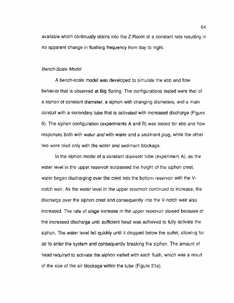
64
available which continually drains into the Z-Room at a constant rate resulting in
no apparent change in flushing frequency from day to night.
Bench-Scale Model
A bench-scale model was developed to simulate the ebb and flow
behavior that is observed at Big Spring. The configurations tested were that of
a siphon of constant diameter, a siphon with changing diameters, and a main
conduit with a secondary tube that is activated with increased discharge (Figure
9). The siphon configuration (experiments A and B) was tested for ebb and flow
responses both with water and with water and a sediment plug, while the other
two were tried only with the water and sediment blockage.
In the siphon model of a constant diameter tube (experiment A), as the
water level in the upper reservoir surpassed the height of the siphon crest,
water began discharging over the crest into the bottom reservoir with the V
notch weir. As the water level in the upper reservoir continued to increase, the
discharge over the siphon crest and consequently into the V-notch weir also
increased. The rate of stage increase in the upper reservoir slowed because of
the increased discharge until sufficient head was achieved to fully activate the
siphon. The water level fell quickly until it dropped below the outlet, allowing for
air to enter the system and consequently breaking the siphon. The amount of
head required to activate the siphon varied with each flush, which was a result
of the size of the air blockage within the tube (Figure 21 a).

30----------------------------~ 65 a
20~
i ""'"' _, /\ '\ I ......... It!
i ·:~~~~AL' I I ~ v ·llO(Q'I wetr · I
-101:------------------~---.J 0 15 30 45
Time (minllktt)
30
~ b /l ' I
20f I I
r
I I
I """"'--I I I A.,._ I ) I
l 10~
I \ \...-------/
/
of
f V·notcn•lr
-10 0 3 6 9 12
TirM (minute.)
30
c 20f
/l I !
r """"'-I
At!Nrvcxr ' I I
~ 101
~~ ' ;; /
' ' -
ot_ /"'"- - --v-noten-"
-10 0 6 9 12
TirM (mirlutn)
Figure 21. Digital data from the bench-scale model experiments: (a} shows the behavior of a siphon constant diameter, (b) represents a siphon that contained a sediment plug in the lowest sump, and (c) shows the behavior of two conduits, the lowest of which contains a sediment plug.

66
The water level through the V-notch weir climaxes at approximately 2.4
em of stage for each flush regardless of the hydraulic head in the upper
reservoir (Figure 21 a), possibly from insufficient resolution of the pressure
transducers at the low water levels used in the experiment. The higher the head
in the upper reservoir required to activate a flush, the longer the flow period
through the weir.
A sediment plug approximately 8 em in length with particle sizes ranging
from 0.3 mm to 1.5 mm was added to the sump of the siphon (experiment B).
As hydraulic head was increased in the upper reservoir, water flowed through
the plug as porous media flow which discharged significantly less than in the
previous experiment without the plug. The stage in the upper reservoir
increased at a faster rate than in the previous experiment without a sediment
plug and rose to a higher head before activating the siphon and flushing out the
entire plug (Figure 21 b). An increase in flow through the V-notch weir was not
observed until the siphon was activated.
A larger diameter tube (1.9 em) was attached to the siphon above the
sediment plug (experiment C). The same experiment was performed, and when
the sediment was breached out of the sump during a flush, it entered the larger
diameter tube. The velocity slowed because of the larger cross-sectional area,
and the sediment agitated in a boiling motion before slowly making its way over
the siphon crest and into the bottom reservoir.
On one occasion, the flow control valve was slowly opened and closed to

67
simulate faster head rises and drops in the upper reservoir, better representing
actual conditions in the cave. The results of this experiment showed that as the
valve was slowly shut to reduce the flow, the sediment plug, which was
churning in the larger diameter tube, quickly fell back into the sump greatly
reducing the flow through the system. The degree of blockage that occurred in
the sump varied depending on how quickly the valve was shut, with rnost of the
fines carried away with the flow and only coarse- and medium-grained
sediments remaining. The slower the valve was closed, simulating a larger drop
in head, the coarser the plug became since the finer particles had time to exit
the system. The coarser-grained plug made piping more difficult, resulting in
higher heads in the upper reservoir.
The final experiment (D) involved attaching a smaller secondary tube
(0.95 em) containing the sediment plug to the main flow tube (Figure 5c). A
faster recharge rate was used for this experiment because flow through the
main tube occurred continuously due to its configuration. Stage levels rose in
both reservoirs continuously until sufficient hydraulic head was achieved to
breach the sediment plug (Figure 21 c).
Analytical Methods
Hydrograph Analysis
Analyses of the 1992 Big Spring hydrograph recession curve from
several flushes were attempted using the method proposed by Mijatovic (1968),

68
but because of the initial conditions placed on stage-data collection at the
spring (a data point is collected when the stage changes by +I· 0.03 m), each
recession curve consisted of only six to eight data points. This was considered
to insufficient and the results unreliable. To solve this problem, the datalogger
at Big Spring was reprogrammed in November 1992 to collect high frequency
stage data, which, after the first flush of 1993, would collect 2000 stage records
at one minute intervals followed by 5000 records of normal data collection. This
resulted in 70 to 100 data points present in each recession curve.
Total precipitation and snow measurements were only available on a
daily basis for the study area. Since several flushes occur within a one-day
period, it is difficult to correlate recharge to the flow at Big Spring because it is
impossible to know exactly when any rain fell or snow melted. Also, the
recharge into the Z-Room is probably a release from storage of the karst
aquifer and not from any individual precipitation event. Therefore, the flood
pulse technique introduced by Ashton (1966) and Wilcock (1968) that correlates
aquifer recharge to response could not be utilized. Instead, the method
introduced by Maillet (1905) and later modified by Mijatovic (1968) and Bonacci
(1993) that analyzes only the spring recession curves to determine the
hydrodynamic regime of a karst aquifer was employed.
Hydrographs were chosen for analysis from the set of high frequency
data on the basis that the recession went smoothly from peak to base flow.
Many of the Big Spring hydrographs posess double or triple peaks before

reaching base flow conditions which could not be used in this analysis. A
representative hydrograph is shown in Figure 22, with the results from all
studied hydrographs tabulated in Appendix C.
69
The Big Spring hydrographs that were studied appeared to posess three
dominant flow regimes within the karst aquifer. The overall discharge curve for
the representative hydrograph (Figure 22) can be described by the equation:
a, = 0.87e'74"11 + 0.30e'20
"61 + 0.07e'221 (8)
The total initial yield (001 ) is 1.413 m3/s, which is the onset of discharge from
large diameter karst conduits. This flow is represented by the first term in
equation (8) and continues for 17 minutes, discharging 796 m3 (65%) of water.
The second term represents the discharge from smaller diameter conduits and
open fissures and occurs for 26.1 minutes releasing 344 m3 (28%) of water.
The final term in the equation represents the flow from small fissures and
cracks. This section of the hydrograph has the lowest slope and consequently
the slowest discharge, releasing 86 m3 (7%) in 43 minutes. This results in a
recovery time of 86.1 minutes. The shape of the hydrographs (steep segments)
and the magnitude of the aquifer response time (less than two hours) initially
classify Big Spring as being the outlet of a fast response, conduit flow aquifer.
The total volume discharged during the representative flush was
2082 m3. Of this total, 856 m3 was the base flow discharged and 1226 m3 was
the volume delivered from the flush. This indicates that the flush volume is 1.5
times greater than the base flow which may provide information regarding the

10~-----------------------------------
-~ ;;' :,
E Q I - OT
"' ~ 1 f ~ i 15 : ""a.nr ................ . o · I -' I
I I .I •
o,.f.... . .. . . . .. t.. .. .. .. ~IY:~5?~::-~a~,.=~·:o7~e~··.,..at ..... t..:.:....,J V,=796 m3 I V:z=-344 '0,3 ...... 1
• 3
.
a. ------...!.------- __ .lft::!l_s_m_ __________ ._
70
V,=856 m3
3~.1.~5;;:;90~--;3;::;3-:. 1:::690-:::--::33::--.1-::7~90~-3-3 ...... 18_9_0 __ 33-.1"-9-90---3-3.-20_9_0 __ 3_3j.2190
nme (days)
0.,=1.413 m'ls Oor0.540 m3/s a.,=0.240 m'ls a. =0. 166 m3/S
Total flush volume,12.26 m3
Total base flow volume=856 m3
1,=0.0598 days=86. 1 m1nutes
Figure 22. Representative hydrograph recession limb analysis for Big Spring in 1993 showing three distinct flow regimes. The volume contribution from each flow regime and recovery time are also presented.

71
underlying karst system.
The depletion coefficients (k) decrease as the volume contribution from
each flow regime decreases. The initial flow response, representing large
diameter conduits, has a value of k equal to 7 4.1; the second response from
smaller diameter conduits and open fissures has a depletion coefficient of 20.6,
and the final flow regime representing small fissures and cracks has a depletion
coefficient equal to 2.2.
Spectral analysis
A time-stage data set for the Z-Room and Big Spring during days 103 to
105.5 (April12-14, 1992) was chosen for analysis because of the well defined
ebb and flow behavior (Figure 23). The Z-Room stage is divided by ten so that
both the cave and spring time series can be viewed together. The chosen time
period is near the middle of the ebb and flow season (February through May)
and is representative of the typical hydraulic flush behavior displayed between
Lilburn Cave and Big Spring.
Two types of flow regimes have been identified within this system in
Figure 23. In sections 1 and 3, the cave-spring relationship is quasi-linear, as
indicated by single peaks of fluctuating levels rising and falling at the Z-Room
instantaneously followed by a similar response at the spring. Sections 2 and 4,
however, suggest nonlinear behavior. Both Z-Room and spring stage levels
display multiple peaks decreasing in magnitude until a minimum stage at the Z-

1.5
0.5
Section J Seclion2
;
I :. : -. ·.- ·'-
103.5
I I I I I I
104.0
'
I I
I Seclion 3 I k----~
I I I I
'.f;
J \._ : ~
Time (days)
Big Spring stage -- Z·Room slage/10
I Section 4 I f'----;
I I
I~\ 105.5
Figure 23. Time-series data section representing the stage level fluctuations of Lilburn Cave (Z-Room) and Big Spring for days 103 to 105.5 in 1992. Quasi-linear behavior occurs in sections 1 and 3, while nonlinear behavior is present in sections 2and4.

Room is reached, which is approximately two times lower than the average
minimum stage height. At this point, the stage level in the Z-Room rises and
reassumes linear behavior, while the spring maintains a constant base flow.
73
To perform a spectral analysis on the time series data, the interpolation
method of kriging was used to produce equally spaced data points. Information
regarding the number of data points in each section shown in Figure 23 and
their interpolated time increments are listed in Table 8. Each section has a
slightly different time interval because both the cave and the spring had a
different number of initial data points. To minimize the amount of computer
generated or deleted points in order to acquire an equal number of points for
each section, the time increments (dt) were independently chosen for each data
set.
Spectral analysis was also performed for days 48 to 50 (February 17-19,
1993) on the Z-Room and Big Spring stages for comparison to the 1992 data.
Because of the frequency of flushes during the 1993 season, most of the time
series data strongly suggests nonlinear behavior, with few indications of quasi
linear flow regimes. The data set shown in Figure 24 is divided into two quasi
linear (sections 6 and 8) and two nonlinear data sections (5 and 7) with the z
Room stage divided by 10 for better comparison of both the cave and spring
time series. The interpolated data is shown in Table 8.
Lastly, spectral analysis was performed on a high, sustained flow section
of the 1993 time-series data, shown in Figure 25 to determine if a different

Table 8. lnte1polation data for data sections represented in Rgures 22,23 and 24.
Data Beginning Ending Total lim& Number of Number of Time ParU1ion location lim& tlmo (days) points before points alter Increment Number (days) {days] •nterpolation inlerpolalion dl (in days)
Z-Room 103.1717 103.4755 0.3038 63 50 0.0062
Big Spring 103. I 719 103.4 752 0.3033 40 50 0.0062
2 Z-Room 103.4759 103.8004 0.3245 83 56 0.0059 Big Spring 103.4750 103.8054 0.3304 42 56 0.0059
3 Z-Aoom 104.3490 104.5830 0.2340 54 40 0.0060 Big Spring 104.3503 104.5824 0.2321 33 40 0.0060
4 Z·Room 104.8071 105.1797 0.3726 110 70 0.0054 Big Spring 104.8090 105.1833 0.3743 50 70 0.0054
5 Z-Room 48.3620 48.5844 0.2224 72 48 0.0046 Big Spring 48.3670 48.5833 0.2163 35 48 0.0046
6 Z-Aoom 48.5844 48.9004 0.3160 69 48 0.0067 Big Spring 48.5833 48.9052 0.3219 36 48 0.0067
7 Z-Aoom 49 1618 49.4870 0.3252 102 74 0.0044 Big Spring 49.1667 49.4920 0.3253 57 74 0.0044
8 Z-Aoom 49.4870 49.6667 0.1797 49 38 0.0047 Big Spring 49.4920 49.6667 0.1747 30 38 0.0047
9 Z·Room 7.3425 7 8410 0.4985 27 26 0.0194
B1g Spring 7.3384 7.8333 0.4949 25 26 0.0194
Data partitions 1 lhrough 4 shown in Figure 23. Data partitions 5 through 8 shown in Figure 24. -....j Data partition 9 shown in Figure 25. .j:>.
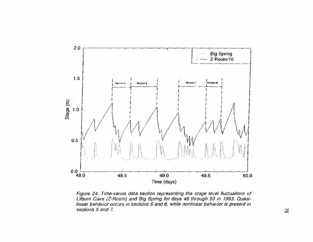
2.0
1.5 j j Section 5
I j
j
I I s.c-· 1 I I I
----Secoon 1
Big Spring Z-Room/10
1Ssclion8
~ 1.0 I I I
I I I I I I <tl
(i)
0.5
0.0 48.0
0 ·:-.
48.5 49.0 Time (days)
I\ I' i\ ) ·~
49.5 50.0
Figure 24. Time-series data section representing the stage level fluctuations of Lilburn Cave (Z-Room) and Big Spring for days 48 through 50 in 1993. Quasilinear behavior occurs in sections 6 and 8, while nonlinear behavior is present in sections 5 and 7.

~
E. Q> 0> <t! -YJ
2.0 ~--~----~--------------~----~~------~----~----,
1.5
1.0
!l 0.5
0.0 '----~----~ 7.0
,. :.[\
I I I I I I I I
Section 9
7.5 Time (days)
· ·· Big Spring stage --- Z-Roomstage/10
8.0
Rgure 25. Time-series data section representing stage levels of Lilburn Cave(Z· Room) and Big Spring during a high, sustained flow period in 1993.

process was operating than when ebb and flow behavior exists. The
interpolated data also appears in Table 8.
Power Spectra
77
The power spectra for the 1992 Z-Room and spring time-series data
section (Figure 23) for the two quasi-linear sections (1 and 3) are shown in
Figure 26a,b. These similar spectra are all relatively smooth, decreasing curves
which strongly suggest a linear to quasi-linear system. Both sets of power
spectra display slight irregularities regarding the smoothness of the curves,
which are attributed to noise within the data. The power spectra for the two
nonlinear sections (2 and 4) are shown in Figure 26c,d. Both power spectra are
fluctuating similarly with an apparent decreasing trend. The variations show an
average exaggeration of the power spectra of about 1 0 times, with one spike at
the spring in section 2 deviating by almost 100 times. This is characteristic of
nonlinear behavior.
The power spectra for the 1993 Z-Room and Big Spring time-series data
section (Figure 24) produced results similar to the 1992 analyses. The power
spectra for the two quasi-linear sections (6 and 8) shown in Figure 27 are
relatively smooth, decaying curves, while the two nonlinear sections (5 and 7)
fluctuate highly as the curve decays.
The power spectra for the high, sustained flow period in the Z-Room and
Big Spring (Figure 28a) are decaying curves with great variability.

78
a "'
b 10" ~ ,..I
p ~~~~ ,.,.
l f "' > l' . ~ ... ~ j ~~~r ~ ' ! . lit t ~ ~ g' 10'1~ ~ 11)-1
m .J lit g. u; 10""
I ' , .. Q ..• ,, ().I! "
.., " '" •• ,., ,, , ..
0 '·"' " '" " "' " "' .. '" '·' F'requency (1/dl) Frequency (Hdt)
d ·~~--------~~--------~
rQ' \<
'
FreQuency (1/dl) Frequency (1/dl)
Figure 26. Power spectra of the four time-series data partitions in Figure 23. The smooth nature of graphs (a) and (b) [data partitions 1 and 3, respectively] indicates quasi·linear behavior, while the variable pattern of graphs (c) and (d) [data partitions 2 and 4, respectively] is a nonlinear response. Notice the linear relationship between the Z-Room and Big Spring in all four data partitions.

79
a ,. b
10'. ,,,
·~· i
\ 1' ~~~
J{lol~ f 1 ; '"'\ \ l 13 f 1
i '"'\ 1 ~ )()"'~ \ l ~ '
!\ l&l~ 1 I ···I l
El ~ j l I • t & ;
' ill l .... ' .... ~ l .
' ' \ ...
' '"' "' "' " Oll " a.ll "' .. , ,, • •• • '" " '" " "' "' 0.33 .. . .. ., Fre<wef'lC)' ( 11d1) F rf;!qtlency f l!dl)
d c
:I •• I ,,, t I~ l
? ~~·~ '"'
~ 10''~ l . . I * t
• r ' !! I l ~~~~ l ~ "'I ~ f I ~ r I
I n '''I I ~ ... \ ~ . ' ' • ' l ii' t i 0 Jo-<l ~
Vi ~~~ I "' ' '~'l I i
~~ ltl~ f ""I
r ~ ... ,,, . ' ~ o- ' "' " "' "' "' .. "'' " • '" . ' OH " 0~, " "' .. "' •.. Freouency (1/dt) FteqVency (11d1)
Figure 27. Power spectra of the tour time-series data partitions in Figure 24. The smooth nature of graphs (a) and (b) {data partitions 6 and 8, respectively] indicates quasi-linear behavior, while the variable pattern of graphs (c) and (d) [data partitions 5 and 7, respectively] is a nonlinear response. Notice the linear relationship between the Z·Room and Big Spring in all four data partitions.

6 ~
! ~
" 11 ~
w
"' !!! d)
b I(Jo·•.-------------------------------.
a ~r-------------------------.
...
"''
"'
·~
, .
... m•
'
~'\
v~~, ~/
!Ol() Ot» HI tll' Ol Olj OJ on O . .f O.f!i lH
Frequency (Hdt)
'\ c
"'
c~A"' " '" " ., " "' "
,., Frequency (1/dl)
"
om,---------------------------,
OOJ
Qj 0005 E ~
0
"OJ~. ----+-----:------,.:-------~. -----;;, • .-------;, Time (d!l
Figure 28. Graph showing (a) power spectra, (b) transfer function, and (c) kernel function of the high, sustained flow period in 1993 shown in Figure 25. The variablifty of all three spectral analyses indicate nonlinear behavior. OJ
0

81
The power spectra for all the time-series studied show the spring always
occurring at a lower spectra than the cave. This is from attenuation of the input
noise occurring within the system, and is common in karst systems because of
the complexity of flow paths that can smooth out initial noise (Andricevic,
personal communication, 1992).
Transfer functions
The transfer function represents the degree of attenuation of the input
noise that is occurring within the system. The transfer functions for the 1992
data are shown in Figure 29. Both linear data sets have transfer functions that
trend horizontally, with slight variations due to noise, and level off at
approximately 1 o·'. The transfer functions for the nonlinear sections also tend to
remain around 1 o·', but as with the power spectra, show extreme variability and
verify the presence of nonlinear behavior.
The transfer functions for the 1993 data (Figure 30) are also similar to
that of the 1992 data. The quasi-linear data sections trend horizontally at 1 o·' at
low frequencies, then increase to 10°. The nonlinear data sections appear to
fluctuate around 1 o·'.
The transfer function for the high, sustained-flow data section (Figure
28b) is highly variable, averaging at 4 X 10·2, slightly more variation than the
ebb and flow, out-of-phase data sets.

a b ''" -~-- -~---~--------, '"'.---~-
10 '0!---70 01
,_-=,e--, --oc0
,c-, --,.01,---0,-,,~, ~. 1o--c0,_,,---
0,.,
4,.--,
0,.,,.----}
0 ,
Frequency (1/dl) Frequency (1/dl)
... , ..
111 'o nre 01 Ol:S nz ou OJ on o• o.n cu Frequency f1tdl) F1equeocy (1/dt)
Figure 29. Transfer functions of the four time-series data partitions in Figure 23. The relatively smooth transfer functions represented in graphs (a) and (b) [data partitions 1 and 3, respectively} trend horizontally at approximately to-1 with slight variations due to noise, indicating quasi-linear behavior. The highly variable transfer functions in graphs (c) and (d) [data partitions 2 and 4, respectively] verify the presence of nonlinear behavior. co
I\)

...
Frequency fl!OtJ
•••
b ·~.-------------~-------------
...
····,f.---,.=.,-----, • .,., ......,.••""• -.,--.,..,---• .,--• .,,-.,... .• -.-.. _J ••
Frequency (1/d!J
d ••.-------------------~
IOI.(J.!-7.,;;;1ll--;;Q";-I ~.l:;-l --,c.,o-;,c::,;-cO~l-;;O;;;JS--;;D";-< --;C .. ;;-, -o!., Frequency {1/dl}
01 O.:U 0.1 IUJ <U 0.4$ 0.3
Frequency (1/d1}
Figure 30. Transfer functions of the tour time-series data partitions in Figure 24. The relatively smooth transfer functions represented in graphs (a) and (b) [data partitions 6 and 8, respectively] trend horizontally at approximately 1U' with slight variations due to noise, indicating quasi-linear behavior. The highly variable transfer functions in graphs (c) and (d) {data partitions 5 and 7, respectively} verify the presence of nonlinear behavior.

84
Kernel functions
The kernel functions for the 1992 data sections are displayed in Figure 31. The
kernel functions for the quasi-linear sections fluctuate slightly above and below
zero by approximately +1- 0.06 in section 1 and +1- 0.1 in section 3, with both
levelling off at zero after six time units (approximately 52 minutes). The kernel
functions for the nonlinear sections fluctuate slightly above and below zero by
approximately +1- 0.02, never stabilizing to zero as in the quasi-linear sections.
The kernel function for the first quasi-linear data section of the 1993 data
(Figure 32a) greatly fluctuates around zero, with a variability of +1- 0.06,
whereas the second quasi-linear data section (Figure 32b) smoothly decays
after an initial rise to 0.13, dropping below zero after seven time units
(approximately 47 minutes). The kernel functions for the two nonlinear data
sections (Figure 32c,d) fluctuated around zero by +1- 0.01. The kernel function
for the high, sustained flow data section (Figure 28c) fluctuates greatly around
zero, ranging from +0.015 to -0.01.

a b ... on
., 000 ... ... . ..
~ ... ~ ... • "
.., E
~ a; c ;;;
"'
c • • ~
" " ..,., ..,., .., .. .... . ..
~-060 10 " .. " .., .. ,
10 " .. ,. T1me (dtl Ttme (dl}
c d ... . .., ..,
om
001 r o.oa
v NV ~ 001
~ ~dOCS .... , ~
" • '"' "."'" ....
-00) .(lOll
"""' """'• 10 " .. " .. • " " ,.
" Time !dli T!IfW (dt)
Figure 31. Kernel functions of the tour time-series data partitions in Figure 23. The quasi-linear nature of graphs (a) and {b) {data partitions 1 and 3, respectively] show the kernel functions stabilizing after six time increments {approximately 52 minutes], which is the time necessary tor one complete flush cycle to occur. The graphs in (c) and (d) [data partitions 2 and 4, respectively] never appear to stabilize, implying nonlinear behavior.
II
..
"'
"
CD CJ1

~ .. E • "'
~ .. 0
~ ~
a b
·:: \ '"
"" .,
... "" B . .,
,;
""
~ ~~ ~ E • • ~
""' ""
.. , ... ""
.. • ,,
" " " • ,. " .. T•me (d1) Time (dt}
c d ... "'
'"' "" •••
""' ~ 0
,; " E
~ ·OOl
om ... ""' '"
"" ....
• " " " • '' " " " JO
T1me !dl) T1me (dt)
Figure 32. Kernel functions of the four time-series data partitions in Figure 24. The nonlinear behavior occuring in (a) [data partition 6] may indicate chaotic behavior. The quasi-linear nature of graph (b) (data partition 8] show the kernel function stabilizing after seven time increments [approximately 47 minutes], which is the time necessary for one complete flush cycle to occur. The graphs in (c) and (d) [data partitions 5 and 7, respectively] never appear to stabilize, implying nonlinear behavior.
J ,. "
" "'

CHAPTER 4
DISCUSSION
87
This section will discuss the implications of the time-series, hydrograph
and spectral analyses regarding the underlying karst geometry of the Lilburn
Cave-Big Spring system. These results, along with observations of the bench
scale models and knowledge of sediment transport, will be combined to
produce a model that best describes the mechanism of ebb and flow behavior
within the Lilburn Cave-Big Spring system.
Chemistry
Gross chemistry analyses of water samples collected from Redwood
Creek upstream of the karst area and at Big Spring show significantly higher
Ca2+, HC03", and pH in the spring's water (Table 5), confirming that the water
flowed through a carbonate system after its surface flow. The water at Big
Spring is more saturated with respect to calcite and dolomite than at Redwood
Creek which indicates that active dissolution of the carbonate material is
occurring. The extent of dissolution of the karst could not be resolved due to
the short time period of this study. According to Sweeting (I 973), the ebb and
flow behavior of a karst spring should be waning from dissolution of the
carbonate material because, with time, all ebb and flow springs will become
normally-flowing karst springs.

88
Stream gaging
Stream gaging at Big Spring to relate stage measured in the datum pool
to discharge was performed to produce a rating curve (Figure 14) and is
represented by equation (7). Sara (1977) also produced a rating curve for
stage-discharge relationships at Big Spring; the stage was measured using a
Stevens recorder and was based from a different datum. Sara's curve has a
similar shape but is shifted slightly to the right so that higher discharges are
obtained for a given stage. The rating curve used in the current study was
developed during 1992 and 1993 and may not be valid for future work.
Time-series observations
The cyclic discharge observed in the Big Spring time-series represents
ebb and flow behavior. The instantaneous response of the spring to Z-Room
water level drops (Figure 15) indicates that the system is completely filled with
water and the rise at the spring is a pressure response when the Z-Room
achieves a significant amount of hydrostatic head to activate, or flush, the
system. The instantaneous response is observed in the 1992 and 1993 stage
hydrographs of the Z-Room and Big Spring, which are the only digital records
that are available of both input and output. Stage responses from both locations
that were obtained by using a Stevens strip chart recording system for two days
in April 1970 also show an instantaneous response (Moore and Sullivan, 1978),
confirming that this behavior is not a recent phenomena.

89
The rate of rise of the Z"Room stage in the 1992 time-series appears to
decrease when water levels in the River Pit begin to rise (Figure 16a). This is
probably because of the lower influx of water from the River Pit to the Z-Room
resulting from the backup. This change in slope is not apparent in the 1993
data (Figure 16b), possibly because of additional recharge from the Pebble Pile
Creek sinkhole, which enters Lilburn Cave between the River Pit and the Z
Room. Recharge from Pebble Pile Creek was not evident in the spring of 1992,
indicating that the large amount of precipitation in 1993 opened a direct conduit
connection between the sinkhole and Lilburn Cave.
Hydrograph analysis
The hydrograph analysis (Figure 22) indicate a predominantly conduit
flow aquifer system between the Z-Room and Big Spring, with approximately
two-thirds of its flow discharging from large diameter conduits, one-fourth from
open fissures, and the remainder from small fissures and fractures. The
hydrograph analysis only offers information on the portion of the aquifer
between the Z-Room and Big Spring, and does not supply knowledge regarding
the storage of the entire karst aquifer.
The magnitude of the depletion coefficients (k) are much higher than the
generalizations earlier stated by Mijatovic (1968). This is because of the high
frequency of flushes that occur at Big Spring. Aquifer response time for Big
Spring is approximately one hour, as opposed to several days tor springs used

90
in Mijatovic's study. The k values for each of the flow regimes recognized at Big
Spring differ by approximately an order of magnitude, which is consistent with
the values obtained in Mijatovic's study. The depletion coefficients obtained for
the first subregime representing large conduit discharge are smaller than
expected, possibly because the peak flow is being damped resulting in cyclic
discharge. Instead of one typical large surge occurring at the Big Spring from a
recharge event, several smaller ones result.
The ratio between peak and base flow discharge for Big Spring is
approximately 5:1. Quinlin (1990) suggested that this would indicate the
presence of a diffuse flow aquifer. The extremely quick aquifer response times
for a complete flush to occur at Big Spring (less than 2 hours), however,
indicate a conduit flow system. This discrepancy in results could be from the
ebb and flow behavior suppressing the peak discharges.
Spectral analysis
Spectral analysis indicated both quasi-linear and nonlinear flow behavior
present within this cave-spring system. The nonlinear behavior could be the
result of recharge entering the Z-Room more quickly than can be handled
linearly, or it could be from the unpredictability of the stochastic element acting
within the system causing the ebb and flow behavior. The Z-Room reaches a
minimum and begins rising when the hydrostatic head is low and the system
has become stable again. During this time of nonlinear behavior at the input (Z-

91
Room), the output (Big Spring) continues to respond linearly.
The input and output spectra for a true linear system would always level
off at approximately the same value, respectively, and appear nearly identical in
shape. For the Lilburn Cave-Big Spring system, the cave always levels off at a
different spectrum, as does the spring (Figures 26, 27 and 28a), with both
spectra behaving similarly. This indicates that there is a variable acting within
the system causing the input to behave stochastically, although the system
responds linearly between input and output. This stochastic behavior is thought
to be the result of flow path blockage due to a variable sediment load present
within the system during the ebb and flow season. When sufficient hydraulic
head is reached, the system is breached and the flow cycle resumes.
The transfer functions (Figures 28b, 29, and 30) show the degree of
attenuation of the initial input behavior within the system. The quasi-linear and
nonlinear data sets for both years trend horizontally at approximately 1 o-1,
indicating that the cave has ten times more variation than the spring in both
types of flow regimes. Most of the quasi-linear transfer functions also show a
slight upward trend at higher frequencies. This could indicate either minimal
inputs into the system (occurring from storage or fracture drainage), or residual
effects at the spring from the previous flush because of the short lag time
between flushes (approximately 45 to 60 minutes}.
The kernel functions (Figures 28c, 31, and 32) are almost equally
distributed about the zero axis. This could possibly be due to the draining and

92
filling of the storage and small fractures within the flow paths, creating other
inputs and outputs. The degree to which the kernel functions fluctuate about
zero in Figures 28c, 31, and 32 is not large, suggesting that additional conduit
flow paths are not present. The small variations in kernel functions in both the
quasi-linear and nonlinear data sets also indicates that the system is primarily a
conduit flow aquifer. The kernel functions for the quasi-linear data sections for
1992 (Figure 31 a, b) tend to level off at zero after approximately six time
increments (approximately 52 minutes) and in 1993 (Figure 32a,b) after seven
time units (approximately 47 minutes). This is about the time necessary to
complete one flush cycle (from rise to fall at the spring). This implies that after
one flush, the changes occurring within the system do not significantly affect the
input or output. The amount of the kernel function above and below zero in the
nonlinear data sets are slightly less than that of the linear sections and occur
with a higher frequency. The fluctuations are exaggerated because the
nonlinear kernel functions are plotted on a smaller scale than the quasi-linear
kernel function. The variability of the kernel function along with the fact that they
do not level off at zero strongly suggests nonlinear behavior. Because the
nonlinear sections do not appear to have additional inputs or outputs than the
quasi-linear sections, the change in behavior does not appear to be the result
of an activation of new flow paths at variable water levels.
The kernel function for the first quasi-linear data section for 1993 (Figure
32a) shows a great amount of variability. This is typical of nonlinear behavior,

93
but the power spectra, transfer function, and time-series examinations suggest
the presence of quasi-linear behavior. The ability of a seemingly stable, linear
or quasi-linear system to randomly display nonlinear behavior may be a
transition to a chaotic solution (Drazin, 1992).
The spectral analyses from a period of high, sustained flow (Figure 28) in
1993 strongly suggest nonlinear behavior. However, the triggering mechanism
from ebb and flow, out-of-phase behavior to high flow, in-phase responses may
also be a result of chaos.
There are several factors that govern the transition to chaotic behavior of
a system, the simplest being from critical instability (Drazin, 1992). A system
becomes unstable when a parameter increases or decreases through a critical
value and the system rapidly follows the path of a strange attractor. A chaotic
solution is usually difficult to recognize, and cannot be detected by simply
looking at the time-series. It is also difficult to distinguish a chaotic signal from
noise. Therefore, based on the analysis techniques used in this study, the
presence of a chaotic solution is inconclusive.
Bench-scale model
The results of the bench-scale model are summarized in Table 9 and
are compared to actual observations for the Lilburn Cave-Big Spring system.
Experiment A (siphon model of constant diameter tube, Figure 9a), which is the
most current acceptable explanation regarding ebb and flow springs (Meinzer,

94 Table 9. Hydrologic relationships of the bench-scale experiments and current models explaining ebb and flow springs as compared to the actual behavior observed within Lilburn Cave and at Big Spring.
Model -·· Corn>arioon to Bia Sorina
Ouiputtlaw;- .. in!>Utllaw -....G. Big Sflm9- .......,. .. Z-Roam.,.ge risos.
Var~e,tn n l.ize of the air~ Niluled 1n a Z-Raooo ftuohed ot dif.,.nt hyojn>sllll;c hoods. Sl>h<>n (OOIIItOnt 11-ng 1¥1--roquinsd to-·
d-et') otlush.
Required tho lnttuenee of air irto the aystem at UnlikeJV that air it inOuendng the ebb and flow the ~to CN4111e ana tbb cyde •the outpUt. --Wotord~....,..plugu-modio flow,
Siphoo (or •• oondul) Negligmio ;..,..... in flaw ot tho 01111>Jt while Big Spting - - ""'lliul>lo as z.Room wl.h HdmeM plug otago ihc>uoing 01 the ..... --(constaM damater, .,., S.111, 1977)
Sediment plug -elf·- out. t .. ult-O-nt ol IOdi .. nl dilclllllling ltYough spring, and unliketv ttun 0110119h sedOment io ontet'ing tho- to -the posoogo,
Moy ..... ., t:llanging--d-- Buo - ot Big Spong'"""' oonNnt ttwuoltout"" _, ...... -dog-ot t!Woughout "" yt!Ot. ~ .. Sediment-"" .. ,., •• -.._. vary;no stage ~prior t() fll8hing cxx::ur tn the
$l>llon (or oinglo oondult) atterthe OMet of a flush f'IQUl'ing ~~~g Z-Room. Wlh INICiimont plug hy-.bchoodlotthoinpn.
enteftng targ• diarNter -- Flushing- finer portidoa,.. ot tho Mediul'l'lo to f~ Mdimenta dtpoUed system. wftifti CCJ~UH Mdwnemt were atBigSpmg, oorUined in targ• dllf'IWet ltbe.
A """1M11!1ined aodiment plug..- inlial May e~fn the high 'tage 6ovels that occur m piping to et:tiYate • fkllh mor. difficti\ NIUling thl Z·ROI:Im after a nonhneM flushing cyae. in higher hMdl in the 14JP8' f'6tiltMMr.
Duak:onduil: system Stage li!Mtll: • both the if1X11 and OU'tpU\ toH Big Spmg .,.go hoo a nogigibto rise as 1imJh~ until Mdiment t:~tuo wn brUI:Md. Z~Rootn cta91t ~-
~""""g Similar to dualooOnclul •yw.tem •udl ttud u Big Sflm9-- not in....,.. as Z-Rocm (SWMbng, 1973) stage in c::eve riMa. atage at IPftng l'lles. 1taQe tlMI. ~during the high-flow ponod.

95
1942), did not result in behavior consistent with the phenomena observed in the
Z·Room and at Big Spring. As the water level in the cave rises, the flow at Big
Spring remains constant until a flush occurs, whereas in the model the flow
continually increased over the siphon crest and into the V-notch weir until
sufficient head was achieved in the upper reservoir to fully activate the siphon
(Figure 21 a). The siphon model appears to flush at a different hydrostatic head
depending on the size of the air blockage within the siphon tube. The influence
of air could explain the variable stage levels in the Z·Room that result in a
flush, but the South Seas room, which is directly downstream of the Z-Room
and conveys the discharge to Big Spring, contains water year-round. At least
one conduit was observed in this room by divers during the summer months
(low water level) which exists below the local water table. The water level in the
South Seas room, therefore, does not drop low enough to allow air to enter any
possible conduit leads and break the siphoning action.
Explanations regarding the siphoning action of ebb and flow springs
(Meinzer, 1942; Sweeting, 1973; Bonacci, 1987; Jennings, 1987) all state that
these springs dry up between flows with very consistent flow variations, always
rising to the same maximum and minimum levels. The simple siphon model
constructed in this experiment did not produce these commonly accepted
results. Once the siphoning action began, the flow never completely ceased
through the V-notch weir; it dropped to a minimum when air entered the system
and then slowly increased because of the continual discharge over the siphon

96
crest until the siphon was reactivated, greatly increasing the flow. Consistent
flow variations could not be reproduced in this bench-scale model. The height of
the stage in the upper reservoir required to activate the siphon was a function
of the size of the air blockage that also varied with a constant recharge rate to
the upper reservoir. The Lilburn Cave-Big Spring system is very unique in that
access into the cave allows for the system input to be studied. The results of
this study can therefore be applied to other ebb and flow springs in which the
controlling mechanism may have originally been misinterpreted.
The second experiment (B) in which a sediment plug was placed in the
lowest sump of the siphon (Figure 9b) resulted in porous media flow through
the plug with a negligible discharge through the V-notch weir (Figure 21 b). This
suggests that if a single conduit with a sediment plug was present within the
Lilburn Cave-Big Spring system causing the ebb and flow cycles, as proposed
by Sara (1977), the flow passing through the sediment plug may not be
sufficient to achieve a constant, perennial base-flow stage of approximately
0.15 m at the spring. It may also result in the base level at the spring to be
constantly changing throughout the year from varying degrees of blockage
resulting in changing hydraulic conductivities. This is not observed at Big
Spring; however, it is possible that damping effects of the water level
fluctuations from travel through the karst system, and insufficient resolution of
the pressure transducers may obliterate any effects of varying hydraulic
conductivities of the sediment plug.

97
When sufficient hydrostatic head was obtained in the upper reservoir,
the sediment plug was forced completely out of the system. This indicates that
if sediment were the controlling factor for the cyclic behavior, it must enter a
larger cross-sectional area after being breached from the sump. This area will
have insufficient velocity to force large particles out of the system, causing them
to agitate turbulently until the head in the upper reservoir, or input, drops
sufficiently to resettle the sediment plug in the sump. In experiment C, when the
sediment entered the larger diameter tube during a flush, the turbulent motion
occurred while slowly discharging over the crest and out of the system.
Although the theory was correct, this implied that the size of the larger tube was
not of the correct magnitude to sufficiently slow down the velocity and retain at
least the heavier, larger particles.
The final experiment (D). which involved a secondary tube that contained
the sediment plug, resulted in stage levels in both the upper reservoir and the
V-notch weir rising simultaneously until the sediment plug was breached (Figure
21 c). This does not represent the behavior of the ebb and flow cycles at Big
Spring, but the action is similar to the periods of high, sustained flow where the
stages in the Z-Room and Big Spring rise and fall concurrently.
Best-fit model of Lilburn Cave-Big Spring system
Based on the results of the bench-scale model, the analytical methods,
and the actual behavior observed within the Z-Room and at Big Spring, a

98
generalized representation of the internal geometry of the cave-spring system
was developed and is shown in Figure 33. A single conduit containing a
sediment plug is the best-fit model for this system. The hydrograph analyses
confirmed that the portion of the karst aquifer between the Z-Room and spring
is primarily a conduit flow system, and the spectral analyses did not show
evidence of other significant inputs or outputs.
A sediment plug within this system is thought to be the stochastic
element causing the cyclic flow behavior since large quantities of sediment are
observed in Lilburn Cave with sizes ranging from fines to boulders composed
primarily of granitic materials. The sediment plug probably exists in the lowest
sump of the conduit. When sufficient recharge begins to fill the karst aquifer,
and consequently the Z-Room, the base flow through the plug and at Big
Spring initially increases. The stage in the Z-Room begins to rise when
recharge into the aquifer exceeds the capacity of discharge through the plug.
Eventually, the Z-Room will achieve sufficient hydrostatic head to breach the
plug, displacing the sediment into a significantly larger area above the sump,
suspending the sediment because of a lower velocity. Figure 15 shows the Z
Room stage falling slowly at first, then abruptly dropping several meters. The
initial slow drop is probably a result of the sediment plug starting to pipe and
liquify, allowing flow to increase through the plug. As the water level in the Z
Room drops and flows out the spring, the hydraulic gradient is lowered causing
the largest particles to drop back into the sump from lowered velocity followed

.-----------------------------------700m --------------------------~
Z-Room
??1
.------15-30m-+----~
30m
surveyed- South S s by divers
'
1 possibly ·other leads
Sediment Plug
Figure 33. Proposed model of the Lilburn Cave-Big Spring system. South Seas and a portion of the conduit at Big Spring have been surveyed by divers. The system is assumed to be a single conduit system containing a sediment plug in the sump that stochastical/ y blocks the flow path creating ebb and flow discharge cyd es. A larger crosssectional area is present above the sump that retains much of the sediment because of a lower velocity during a flush. Some fractures and open fissures are probably present throughout the system, as indicated by the hydrograph and spectral analyses.
10m
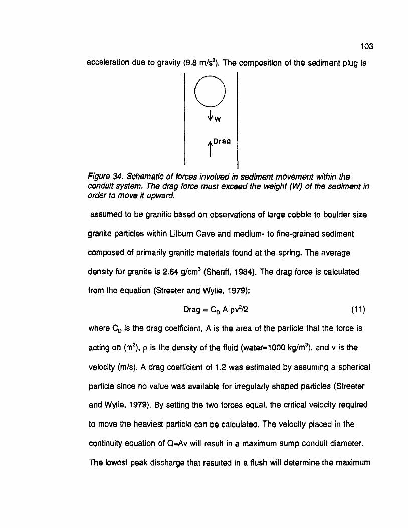
103
acceleration due to gravity (9.8 m/s'l). The composition of the sediment plug is
0 ~w
jorag
Figure 34. Schematic of forces involved in sediment movement within the conduit system. The drag force must exceed the weight (W) of the sediment In order to move it upward.
assumed to be granitic based on observations of large cobble to boulder size
granite particles within Lilburn Cave and medium· to fine-grained sediment
composed of primarily granitic materials found at the spring. The average
density for granite is 2.64 g/cm3 (Sheriff, 1984). The drag force is calculated
from the equation (Streeter and Wylie, 1979):
Drag = C0 A p..;/2 (11)
where C0 is the drag coefficient, A is the area of the particle that the force is
acting on (m2), pis the density of the fluid (water=1000 kg/m3
), and vis the
velocity (m/s). A drag coefficient of 1.2 was estimated by assuming a spherical
particle since no value was available for irregularly shaped particles (Streeter
and Wylie, 1979). By setting the two forces equal, the critical velocity required
to move the heaviest particle can be calculated. The velocity placed in the
continuity equation of Q=Av will result in a maximum sump conduit diameter.
The lowest peak discharge that resulted in a flush will determine the maximum

104
possible conduit diameter of the sump because if the conduit were larger the
velocity would be insufficient to displace the sediment. The lowest peak
discharge in 1993 was 0.673 m3/s (0.34 m stage). Several average particle
sizes were chosen and these results are listed in Table 10. The calculated
diameters assumes all particles are the same size and are spherical.
Realistically, there are probably a wide range of particle sizes and during low
stage flushes the large particles remain in the sump.
Because the conduit size was estimated along with the average sediment
size, Table 10 can only serve as constraints on the possible internal dimensions
for the proposed model explaining the unique ebb and flow behavior that occurs
within the Lilburn Cave-Big Spring karst system. The proposed model consists
of a single conduit with a sediment plug in its lowest sump stochastically
blocking the flow path creating the ebb and flow discharge cycles, with a larger
cross-sectional area above the sump that retains most of the sediment because
of lower velocity.
Table 10. Estimates of maximum sump diameter based on average particle sizes of granitic composition and a C0 of 1.2, using the lowest peak discharge at Big Spring for 1993 (0.673m%).
Particle Size Weight Velocity Discharge Sump Diameter I em\ (N) lm/s \ (mA3/s\ !m\
5 1.69 1.20 0.673 0.85 1 0 13.54 1.70 0.673 0.71 1 5 45.72 2.08 0.673 0,64 20 108.38 2.40 0.673 0.60 30 365.76 2.94 0.673 0.54

CHAPTER 5
SUMMARY AND CONCLUSIONS
105
This work provides an interpretation of the mechanism producing unique
ebb and flow discharge cycles during high runoff periods within the Lilburn
Cave-Big Spring karst system. Hydrograph and spectral analyses of the stage
and discharge time-series data, sediment analyses, and a bench-scale model
were combined to elucidate the internal hydrology of this system.
Earlier observations on Big Spring flows indicated that ebb and flow
behavior was a seasonal phenomenon, only occurring during periods of high
runoff. The addition of the datalogger within Lilburn Cave shows:
• the ebb and flow cycles are the result of an instantaneous
response between a drop in stage in the Z-Room and a rise at the
spring. This suggests that the system is completely filled with
water and the rise at the spring is a pressure response when the
Z-Room achieves a sufficient amount of hydrostatic head to
activate the system.
Previously, two types of flow have been recognized at Big Spring: ebb
and flow and high, sustained flow. These two flow behaviors were based initially
only on the spring output. Correlating the stage data obtained from both the Z
Room and Big Spring dataloggers showed:
• the ebb and flow response between the Z-Room and Big Spring

stages was a 180' out-of-phase response and the high,
sustained flow an in-phase response. The triggering
106
mechanism operating between the two types of behavior may be a
result of chaos.
Because Big Spring is a relatively high-discharge karst spring, it was
initially assumed to contain a conduit-flow aquifer. Hydrograph analyses
substantiated this assumption by indicating that:
• approximately two-thirds of Big Spring's flow discharges from large
diameter conduits, one-fourth from smaller conduits and open
fissures, with the remainder from small fissures and fractures.
The power spectra performed on multiple data sets indicate:
• that it is a nonlinear system, with evidence of quasi-linear behavior
on a smaller scale, and
• both of these flow regimes have a varying input spectra, which is
thought to be the result of sediment stochastically blocking the
flow path,
Transfer and kernel function analyses:
• confirm the presence of nonlinear and quasi-linear flow regimes,
and further indicate that no significant inputs or outputs to the
system exist.
The results of a bench-scale model to simulate the ebb and flow cycles
that occur at Lilburn Cave and Big Spring were compared to the action of a

107
natural siphon (Meinzer, 1942), a sediment plug (Sara, 1977), a conduit with
varying diameters, and a dual·conduit system or reciprocating spring (Sweeting,
1973; Jennings, 1987).
The bench-scale model, in conjunction with the analytical methods and
the actual behavior observed within the Z-Room and at Big Spring, suggest:
• a single conduit containing a sediment plug in the lowest sump
that stochastically blocks the flow path creating ebb and flow
discharge cycles (Figure 32), with
• a larger cross-sectional area is present above the sump that
retains most of the sediment because of a lower velocity.

108
CHAPTER 6
FURTHER WORK
Further work regarding the analyses of the Lilburn Cave-Big Spring
system is required to more concisely determine the mechanism governing the
ebb and flow behavior.
Quantitative dye tracing between the Z-Room and Big Spring during low
flow in the summer months and in ebb and flow mode during the spring runoff
period may indicate if single or multiple conduits, or a siphon, is present by the
shape of the dye recovery curve. The travel time of the dye to the spring
indicates the distance the flow path travels, which may result in a conduit
length.
Samples from various locations from within Lilburn Cave and at Big
Spring were analyzed for ()180 and ao isotopes from 1982 to 1984. In July
1983, multiple samples collected during a single flush (Hess, unpublished data)
at Big Spring showed the following fluctuating d180 values (()D results not
available):
Sampling Time ()180
Low flow -9.2 Increasing flow -11.1 Peak flow -8.2 Ebbing -10.7 Ebbing -9.4 Low flow -8.7 Low flow -9.7

109
The fluctuations may indicate multiple water sources contributing to the flow at
Big Spring. There is, however, questions regarding the accuracy of the
equipment used in 1983 analyses. Therefore, the data is insufficient to conclude
the presence of multiple conduits. Further analyses using isotopes may
therefore be useful to more concisely define the Lilburn Cave-Big Spring
hydrologic system.
The presence of chaos in a quasi-linear or nonlinear system may be
recognized by applying additional nonlinear analysis techniques to determine if
a strange attractor is present, such as constructing a phase portrait or a
Poincare section of the phase plane. The fractal dimension of the attractor can
be used to determine if chaotic behavior is present. If the fractal dimension D is
consistent for various sections of the time-series data, it indicates either a
steady or periodic solution. If D fluctuates, it may indicate a chaotic solution.
More sophisticated spectral methods can be applied to better interpret
the unusual behavior occurring within this karst system. Some of these methods
are maximum entropy spectral analysis (MESA), described by Padmanabhan
(1980), or autoregressive models (ARMA) explained by Kendall and Stuart
(1976) and Jenkins and Watts (1968), can supply better resolution in
interpretation of the results. Analysis of the kernel functions through convolution
as described by Dreiss (1989) for use in karstic aquifers may result in a more
detailed description of the system.
The bench-scale models used in this experiment were of very general

11 0
designs so as to narrow down the possible configurations that may result in the
flow behavior observed in the Z-Room and Big Spring. More detailed models
should be designed to better conclude the mechanisms operating within this
system.

111
REFERENCES
Arfken, G., Mathematical Methods for Physicists (third edition), Academic Press, Inc., Orlando, Florida, 1985.
Ashton, K., The analysis of flow data from karst drainage systems, Trans. Cave Research Group Great Britain, 7(2), pp. 161-203, 1966.
Blackman, R.B. and J.W. Tukey, The Measurement of Power Spectra, Dover Publications Inc., New York, 1958.
Bonacci, 0., Karst springs hydrographs as indicators of karst aquifers, Journal des Sciences Hydrologiques, 38(1 ), pp. 51-62, 1993.
Bonacci, 0., Karst Hydrology, Springer-Verlag, Berlin, 1987.
Bridge, J., Ebb and flow springs in the Ozarks, University of Missouri, School of Mines and Metallurgy, Rolla, Missouri, pp. 17-26, 1924.
Brown, M.C., Karst Hydrology of the Lower Maligne Basin, Jasper, Alberta, Ph.D. Thesis, Department of Geography, University of Alberta, 1970.
Cave Research Foundation Annual Report, internal publication, Fresno, CA, 1984.
Cave Research Foundation Annual Report, internal publication, Fresno, CA, 1992.
Cave Research Foundation Personnel Manual, internal publication, Fresno, CA, undated.
Davis, J.C., Statistics and Data Analysis in Geology, John-Wiley & Sons. New York, 1986.
Drazin, P.G., Nonlinear Systems, Cambridge University Press, 1992.
Dreiss, S.J., Linear kernels for karst aquifers, Water Resources Research, 18(4), pp. 865-876, 1982.
Dreiss, S.J., Regional scale transport in a karst aquifer: 2. Linear systems and time moment analysis, Water Resources Research, 25(1 ), pp. 126-134, 1989.

112
Ford, D. and P. Williams, Karst Geomorphology and Hydrology, Unwin Hyman, 1989.
Gaither,B.E., The relation of spring discharge behavior to the hydrologic properties of carbonate aquifers, M.S. Thesis, Geology, The Pennsylvania State University, 1977.
Halliday, W.R., Caves of California, Report of the Western Speleological Survey, 1962.
Harris, A. and Tuttle, E., Geology of the National Parks, Kendall/Hunt Publishing Company, Dubuque, Iowa, 1984.
Hill, M., Geology of the Sierra Nevada, University of California Press, Los Angeles, 1975.
Jenkins, G.M. and D.G. Watts, Spectral Analysis and its Applications, HoldenDay, San Francisco, 1968.
Jennings, J.N., Karst Geomorphology, Basil Blackwell Inc., New York, 1987.
Kendall, M. and A. Stuart, The Advanced Theory of Statistics (third edition), vol. 3, Hafner Press, New York, 1976.
Linsley, R., M. Kohler, and J. Paulhus, Applied Hydrology, McGraw-Hill, 1949.
MacDonald, G.J., Spectral analysis of time series generated by nonlinear processes, Reviews of Geophysics, 27(4), pp. 449-469, 1989.
Maillet, E., Essais d'hydraulique souteraine et fluviale, Paris, 1905.
Meinzer, O.E. (ed.), Hydrology, McGraw-Hill, New York, 1942.
Mijatovic, B., A method of studying the hydrodynamic regime of karst aquifers by analysis of the discharge curve and level fluctuations during recession, Vesnik Zavada Za Geoloska I Geofizicka lstrazivanja, series B, 8, pp. 41-74, 1968.
Moore, G.W. and G.N. Sullivan, Speleology: The Study of Caves, Cave Books, St. Louis, Missouri, 1978.
Padmanabhan, G., Stochastic Analysis and Modeling of Hydrologic and Climatologic Time Series, Ph.D. Thesis, Purdue University, 1980.

113
Quinlin, J.F., Special problems of ground-water monitoring in karst terranes, in Ground Water and Vadose Zone Monitoring, ASTM STP 1053, D.M. Nielson and A.l. Johnson, eds., American Society for Testing Materials, Philadelphia, pp. 275-304, 1990.
Ross, D.C., Igneous and Metamorphic Rocks of Parts of Sequoia and Kings Canyon National Parks, California,· California Division of Mines and Geology, Special Report 53, 1958.
Rubey, W.W., Settling velocities of gravel, sand and silt particles, American Journal of Science, 5th series, 25, pp. 325-338, 1933.
Sara. M.N., Hydrology of Redwood Canyon, Tulare County, California, M.S. Thesis, Geology, University of Southern California, 1977.
Sheriff, C., Encyclopedic Dictionary of Exploration Geophysics, The Society of Exploration Geophysics, Tulsa, Oklahoma, 1984.
Stevens, G., Intermittent Springs, Trans. Cave Research Group Great Britain, 7(1 ), pp. 3-9, 1964.
Streeter, V.L. and E. B. Wylie, Fluid Mechanics (seventh edition), McGraw-Hill, New York, 1979.
Sweeting, M., Karst Landforms, Columbia University Press, New York, 1973.
van der Kamp, G., Determining aquifer transmissivity by means of well response tests: the underdamped case, Water Resources Research, 12(1 ), pp. 71-77, 1976.
Wentworth, C.K., A scale of grade and class terms for clastic sediments, Journal of Geology, v. 30, pp. 377-392, 1922.
White, E. and W. White, Analysis of spring hydrographs as a characterization tool for karst aquifers, lr!. Proceedings of the Fourth Conference on Karst Geology and Hydrology, pp. 103-106, 1974.
White, J. and S. Pusateri, Sequoia and Kings Canyon National Parks, Stanford University Press, 1949.
White, W., Conceptual models for carbonate aquifers, Groundwater, 7(3), pp. 15-21' 1969.

114
White, W., Conceptual models for carbonate aquifers: Revisited, in Hydrologic Problems in Karst Regions, pp. 176-187, 1977.
White, W., Geomorphology and Hydrology of Karst Terranes, Oxford University Press, 1988.
Wilcock, J.D., Some developments in pulse-train analysis, Trans. Cave Research Group Great Britain, 1 0, pp. 73-98, 1968.

115
APPENDIX A
Representative datalogger data
A representative sample of the raw datalogger data for Big Spring is
shown in Table A 1. The digits at the beginning of each data point (01, 02, etc.)
indicate the location in the datalogger where a particular piece of information
will be stored. The first column (01) is the program that the datalogger reads to
collect certain data, and for Big Spring it is either 120 or 302. A 120 specifies to
record the year (column 02), the Julian day (column 03), and the battery
voltage (column 04). A 302 triggers the datalogger to collect the hour and
minute (column 02), the second (column 03), the stage in feet (column 04), the
water temperature in degrees C (column 05), the electrical conductivity in
mhos/m (column 06), and the air temperature in degrees C (column 07). The
datalogger is programmed to initiate the 302 program every hour and when
trigger levels are exceeded (Table 2), while the 102 program is activated at
midnight of each day. The raw datalogger data is easily translated into ASCII
format through programs in Fortran, Basic, etc., allowing for various graphing or
statistical software packages to be utilized.
The raw data from Lilburn Cave is of a similar format differing only in the
datalogger locations that store the collected variables.

116
Table A 1. Representative raw datalogger data for Big Spring.
01+0120. 02+0092. 03+0150, 04+10.29 01+0302. 02+0000. 03+000.1 04+0.546 05+08,70 06+185.8 07+11.94 01+0302. 02+0100. 03+000.1 04+0.545 05+08.70 06+165.8 07+11.40 01+0302. 02+0200. 03+000.1 04+0.544 05+08.69 06+185.9 07+11.12 01+0302. 02+0300. 03+000.1 04+0.546 05+08.69 06+185.9 07+10.73 01+0302. 02+0400. 03+000.1 04+0.544 05+08,70 06+186.0 07+10.61 01+0302. 02+0500. 03+000.1 04+0,548 05+08.70 06+186.1 07+10.15 01+0302. 02+0600. 03+000.1 04+0.546 05+08.70 06+186.2 07+10.75 01+0302. 02+0700. 03+000.1 04+0.548 05+08.69 06+186.4 07+11. 77 01+0302. 02+0800. 03+000.1 04+0.549 05+08.70 06+186.4 07+14 .33 01+0302. 02+0900, 03+000.1 04+0.565 05+08.70 06+186.5 07+16.63 01+0302. 02+1000. 03+000.1 04+0.560 05+08.72 06+186.6 07+18 .34 01+0302. 02+1100. 03+000.1 04+0.556 05+08.75 06+186.5 07+20.24 01+0302. 02+1107. 03+000.1 04+0. 556 05+08.86 06+186.0 07+21. 29 01+0302. 02+1111. 03+015.1 04+0.553 05+08.75 06+186. 7 07+22.09 01+0302. 02+1200. 03+000.1 04+0.549 05+08.73 06+186.8 07+21.19 01+0302. 02+1300. 03+000.1 04+0.545 05+08.70 06+187.0 07+19.74 01+0302. 02+1400. 03+000,1 04+0.553 05+08.71 06+187.1 07+20.02 01+0302. 02+1500. 03+000.1 04+0.545 05+08.73 06+187.1 07+22.85 01+0302. 02+1600. 03+000.1 04+0.534 05+08. 72 06+187.3 07+2l. 65 01+0302. 02+1700. 03+000.1 04+0. 544 05+08. 7l 06+187.3 07+18.99 01+0302. 02+1800. 03+000.1 04+0.545 05+08.71 06+187.4 07+18.30 01+0302. 02+1900, 03+000.1 04+0.548 05+08.71 06+187.4 07+15.84 01+0302. 02+2000. 03+000.1 04+0.546 05+08. 7l 06+187.5 07+14,17 01+0302. 02+2100. 03+000.1 04+0.548 05+08.70 06+187.6 07+13.69 01+0302. 02+2200. 03+000.1 04+0.550 05+08.71 06+187.7 07+13.12 01+0302. 02+2300. 03+000.1 04+0.5n 05+08.70 06+187,7 07+12.50 01+0120. 02+0092. 03+0151. 04+10. 29 01+0302. 02+0000. 03+000.1 04+0. 551 05+08.70 06+187.8 07+11. 98 01+0302. 02+0100. 03+000.1 04+0.546 05+08.70 06+187.9 07+11. 51
Data used in this study are the property of the Cave Research
Foundation. Requests for the data that have been collected at Lilburn Cave and
Big Spring may be made through:
Dr. John Tinsley Cave Research Foundation-West 1040 Oakland Avenue Menlo Park, CA 94025 ( 415) 329·4928
Dr. John W. Hess Desert Research Institute P.O. Box 19040 Las Vegas, NV 89132·0040 (702) 895·0451

117
APPENDIX 8
Stream Gaging
This appendix presents the raw stream gaging data from Big Spring and
the River Pit along with the discharge calculations that produced the Big Spring
rating curve shown in Figure 14. Big Spring was gaged approximately 15 m
below the weir during five different flow periods and the River Pit was gaged
twice. both using the same Pygmy current meter. A rating curve was not
developed for the River Pit because of an insufficient number of data points.
The raw data for Big Spring are in Table B1, and Table B2 contains the River
Pit data. The mark represents the distance from the shoreline.

Table 81. Stream gaging data tor Big Spring on (a) 05124192, (b) 07114192, (c) 11101/92, (d) 05108/93 {peak discharge], and (e) 05/08193 [ebb flow].
(a) 05124/92
Marl< (m) Distance lm) Depth (m) Area (m"2) Velocity (mls) a (m"31sl
0.000·0.061 0.061 0.15 0.01 0.11 0.00 0.061-0.274 0.213 0.17 0.04' 0.28 0.01 0.274-0.457 0.183 0.20 0.04 0.94 0.03 0.457-0.609 0.152 0.17 0.03 1.00 0.03 0.609-0.762 0.153 0.21 0.03 0.98 0.03 0.762-0.914 0.152 0.17 0.03 0.71 0.02 0.914-1.067 0.153 0.18 0.03 0.57 0.02 1.067-1.219 0.152 0.15 0.02 0.64 0.01 1.219-1.372 0.153 0.20 0.03 0.04 0.00 1.372·1 .524 0.152 0.21 0.03 0.09 0.00 1.524·1 . 676 0.152 0.11 0.02 0.04 o.oo 1.676·1.829 0.153 0.14 0.02 0.00 0.00
Sum of 0 = 0.16 Stage (m) = 0.18
(b) 07/14/92
Mark lm) Distance (m) Deoth lml Area (m"2l Velocrtv (mlsl Q lm"3/s)
0.000-0.254 0.254 0.08 0.02 0.03 0.00 0.254·0.508 0.254 0.15 0.04 0.33 0.01 0.508-0.813 0.305 0.17 0.05 0.29 0.01 0.813-1.016 0.203 0.20 0.04 0.52 0.02 1.016-1.270 0.254 0.20 0.05 0.52 0.03 1 .270·1.549 0.279 0.20 0.06 0.38 0.02 1.549·1. 778 0.229 0.14 0.03 0.18 0.01
Sum of Q = 0.10 Stage (m) = 0.16
118

119
Table 81 (continued). (c) 11/01/92
Mark (m) Distance (m) Depth !m\ Area (r11"2l Velocny (mts) Q (rl1"3/s\
0.000-0.254 0.254 0.06 0.02 0.18 0.00 0.254-0.508 0.254 0.15 0.04 0.22 0.01 0.508·0. 762 0.254 0.17 0.04 0.14 0.01 0.762·1.106 0.254 0.20 0.05 0.67 0.03 1.106·1.270 0.254 0.27 0.07 0.54 0.04 1.270·1.524 0.254 0.27 0.07 0.33 0.02 1.524-1.778 0.254 0.21 0.05 0.10 0.01
Sum of Q = 0.12 Stage (m) = 0.17
(d) 05108/93
Mark (m\ Distance (m) Depth (m) Area (rT1"2) Velocity (m/s) a (rl1"3ts)
0.000-0.305 0.305 0.52 0.16 0.11 0.02 0.305-0.610 0.305 0.52 0.16 0.52 0.08 0.61 0·0.915 0.305 0.58 0.18 1.30 0.23 0.915-1.220 0.305 0.61 0.19 1.50 0.28 1.220·1 .525 0.305 0.67 0.21 1.66 0.34 1.525-1 .830 0.305 0.76 0.23 1.32 0.31 1.830-2.135 0.305 0.73 0.22 1.01 0.23 2.135·2.440 0.305 0.73 0.22 0.31 0.07
SumofO= 1.55 Stage (m) = 0.47
(e) 05108193
Mark (m) Distance (m) Depth lm) Area (rl1"2l Velocny (m/s) a (r11"3/s\
0.000-0.305 0.305 0.21 0.07 0.19 0.01 0.305-0.610 0.305 0.40 0.12 0.33 0.04 0.610-0.915 0.305 0.38 0.12 0.80 0.09 0.915-1.220 0.305 0.44 0.13 1.29 0.17 1 .220·1 .525 0.305 0.44 0.13 0.74 0.10 1.525·1.830 0.305 0.46 0.14 0.67 0.09 1.830·2. 135 0.305 0.37 0.11 0.38 0.04 2.135·2.440 0.305 0.31 0.09 0.23 0.02
Sumo! a= 0.56 Stage (m) = 0.32

120
Table 82. Stream gaging data tor the River Pit on (a) 05123192, and (b) 10131192.
(a) 05/23/92
Mark Distance Depth Area Velocity a Average Q
lml (m) !ml (111"'21 lm/sl lm"3/s) (111"'3/S)
0.000·0. 152 0.152 0.29 0.04 0.10 o.oo 0.152 0.29 0.04 0.05 0.00 o.oo
0.152·0.305 0.153 0.34 0.05 0.11 0.01 0.153 0.34 0.05 0.04 0.00 0.00
0.305-0.457 0.152 0.37 0.06 0.13 0.01 0.152 0,37 0.06 0.09 0.00 0.01
0.457-0.610 0.153 0.46 0.07 0.31 0.02 0.153 0.46 0.07 0.10 0.01 0.01
0.610-0.762 0.152 0.46 0.07 0.32 0.02 0.152 0.46 0.07 0.17 0.01 0.02
0.762-0.914 0.152 0.49 0.07 0.21 0.02 0.152 0.49 0.07 0.20 0.01 0.02
0.914-1.067 0.153 0.52 0.08 0.18 0.01 0.153 0.52 0.08 0.21 0.02 0.02
1.067·1.219 0.152 0.52 0.08 0.13 0.01 0.152 0.52 0.08 0.14 0.01 0.01
1.219·1 .372 0.153 0.52 0.08 0.12 0.01 0.153 0.52 0.08 0.10 0.01 0.01
Sum of Avg a " 0.09 Stage (m)= 0.27
(b) 10/31/92
Mark Distance Depth Area Velocity a Average Q
(m) (m) lm) lm"2l (m/s\ lm-'3/s\ lm"3/s)
0.000·0.025 0.025 0.31 0.01 0.03 0.00 0.025 0.31 0.01 0.04 o.oo 0.00
0.025-0.305 0.280 0.27 0.08 0.09 0.01 0.280 0.27 0.08 0.14 0.01 0.01
0.305·0.61 0 0.305 0.34 0.10 0.08 0.01 0.305 0.34 0.10 0.07 0.01 0.01
0.610-0.915 0.305 0.37 0.11 0.09 0.01 0.305 0.37 0.11 0.11 0.01 0.01
0.915·1.220 0.305 0.40 0.12 0.10 0.01 0.305 0.40 0.12 0.13 0.02 0.01
1 .220·1.525 0.305 0.43 0.13 0.08 0.01 0.305 0.43 0.13 0.08 0.01 0.01
Sum of Avg 0= 0.05 Stage (m) = 0.22

j 21
APPENDIX C
Hydrograph analysis
The data obtained from the Big Spring hydrograph analyses used in this
study are listed in Table C1. The stage data used were from flushes occurring
in 1993 that were collected at 1-minute intervals, resulting in recession limbs
that average 70 to 120 points. The average flow contribution from large
conduits is 62.5%, that from small conduits and open fissures is 33%, and the
remainder from fractures is 4.5%. The volume of water discharged during a
flush was 1.2 to 1.5 times higher than tt1e volume of base flow during the same
time interval.

Table Ct. Data for eight hydrographs analyzed using 1993 high frequency data obtained at Big Spring. V1 represents the flow contribution from large conduits, V2 is due to small conduits and open fissures, and V3 is the discharge from fractures. The total volume discharged as a result of a flush is represented by Vf, while the base flow contribution is Vb.
Slarl Erd Recession Peak Base VI V2 V3 VI Vb Vf/Vb Time Time Time flow flow
(days) (days) {min) (m"31s} (m"3fs) (m"3) {m"3) (m"3) (m"3) (m"3)
10.312 10.358 66 0.90 0.15 455 274 31 760 580 1.3 (60%) (36%) (4%)
33.159 33.219 86 1.41 0.17 796 344 86 1226 856 1.4 (65%) (29%) (7%)
34.232 34.295 90 1.16 0.16 650 368 50 1068 888 1.2 (61%) (34%) (5%)
43.184 43.244 86 1.21 0.17 560 410 42 1012 862 1.2 (55%) (40%) (5%)
51.208 51.268 70 1.36 0.18 740 203 50 993 743 1.3 (74%) (21%) (5%)
51.735 51.781 66 1.34 0.17 617 368 90 1075 692 1.5 (58%) (34%) (8%)
64.835 64.877 61 1.22 0.21 579 400 9 988 780 1.3 (59%) {40%) {1%)
64.663 64.73 120 1.51 0.18 1094 460 35 1589 1070 1.5 (68%) (30%) (2%)
t\J t\J