arX

iv:s

olv-

int/9

9070

11v1

8 J

ul 1

999

Spectral decomposition for the Dirac system

associated to the DSII equation

Dmitry E. Pelinovsky and Catherine SulemDepartment of Mathematics, University of Toronto

Toronto, Ontario, Canada, M5S 3G3

Abstract

A new (scalar) spectral decomposition is found for the Dirac system in two dimensionsassociated to the focusing Davey–Stewartson II (DSII) equation. Discrete spectrum in thespectral problem corresponds to eigenvalues embedded into a two-dimensional essential spec-trum. We show that these embedded eigenvalues are structurally unstable under small vari-ations of the initial data. This instability leads to the decay of localized initial data intocontinuous wave packets prescribed by the nonlinear dynamics of the DSII equation.

submitted toInverse Problems

1 Introduction

Gravity-capillary surface wave packets are described by the Davey–Stewartson (DS) system [1]which is integrable by inverse scattering tranform in the limit of shallow water [2]. In this paper,we study the focusing DSII equation which can be written in a complex form,

iut + uzz + uzz + 4(g + g)u = 0,

2gz −(

|u|2)

z= 0, (1.1)

where z = x+ iy, z = x− iy, u(z, z, t) and g(z, z, t) are complex functions. This equation appearsas the compatibility condition for the two-dimensional Dirac system,

ϕ1z = −uϕ2, ϕ2z = uϕ1, (1.2)

coupled to the equations for the time evolution of the eigenfunctions,

iϕ1t + ϕ1zz + uϕ2z − uzϕ2 + 4gϕ1 = 0,

− iϕ2t + ϕ2zz + uzϕ1 − uϕ1z + 4gϕ2 = 0. (1.3)

The DSII equation was solved formally through the ∂ problem of complex analysis by Fokasand Ablowitz [3] and Beals and Coifman [4]. Rigorous results on existence and uniqueness ofsolutions of the initial-value problem were established under a small-norm assumption [5]. Thesmall-norm assumption was used to eliminate homogeneous solutions of equations of the inversescattering which correspond to bound states and radially symmetric localized waves (lumps) of theDSII equation. When the potential in the linear system becomes weakly localized (in L2 but notin L1), homogeneous solutions may exist and the analysis developed in Ref. [5] is not applicable.

The lump solutions were included formally in [3], where their weak decay rate was found,u ∼ O(R−1) as R =

√x2 + y2 → ∞. This result is only valid for complexified solutions of the

DSII equation (when |u|2 is considered to be complex). The reality conditions were incorporatedin the work of Arkadiev et al. [6] where lumps were shown to decay like u ∼ O(R−2). Multi-lumpsolutions were expressed as a ratio of two determinants [6], or, in a special case, as a ratio of twopolynomials [7] but their dynamical role was left out of consideration.

Recently, structural instability of a single lump of the DSII equation was reported by Gadyl’shinand Kiselev [8, 9]. The authors used methods of perturbation theory based on completeness ofsquared eigenfunctions of the Dirac system [10, 11]. A similar conclusion was announced by Yurovwho studied Darboux transformation of the Dirac system [12, 13].

In this paper, we present an alternative solution of the problem of stability of multi-lump solu-tions of the DSII equation. The approach generalizes our recent work on spectral decomposition ofa linear time-dependent Schrodinger equation with weakly localized (not in L1) potentials [14]. Wefind a new spectral decomposition in terms of single eigenfunctions of the Dirac system. Surpriselyenough, the two-component Dirac system in two dimensions has a scalar spectral decomposition.

2

In contrast, we recall that the Dirac system in one dimension (the so-called AKNS system) has awell-known 2 x 2 matrix spectral decomposition [15].

Using the scalar spectral decomposition, we associate the multi-lump potentials with eigen-values embedded into a two-dimensional essential spectrum of the Dirac system. Eigenvaluesembedded into a one-dimensional essential spectrum occur for instance for the time-dependentSchrodinger problem [14, 16]. They were found to be structurally unstable under a small variationof the potential. Depending on the sign of the variation, they either disappear or become resonantpoles in the complex spectral plane which correspond to lump solutions of the KPI equation [14].

For the Dirac system in two dimensions, the multi-lump potentials and embedded eigenvaluesare more exotic. The discrete spectrum of the Dirac system is separated from the continuousspectrum contribution in the sense that the spectral data satisfy certain constraints near theembedded eigenvalues. These constraints are met for special solutions of the DSII equation suchas lumps, but may not be satisfied for a generic combination of lumps and radiative waves. As aresult, embedded eigenvalues of the Dirac system generally disappear under a local disturbance ofthe initial data. Physically, this implies that a localized initial data of the DSII equation decaysinto radiation except for the cases where the data reduce to special solutions such as lumps.

The paper is organized as follows. Elements of inverse scattering for the Dirac system arereviewed in Section 2, where we find that the discrete spectrum of the Dirac system is prescribedby certain constraints on the spectral data. Spectral decomposition is described in Section 3 withthe proof of orthogonality and completeness relations through a proper adjoint problem. Theperturbation theory for lumps is developed in Section 4 where some of previous results [8, 9] arerecovered. Section 5 contains concluding remarks. Appendix A provides a summary of formulasof the complex ∂-analysis used in proofs of Section 3.

2 Spectral Data and Inverse Scattering

Here we review some results on the Dirac system (1.2) and discard henceforth the time dependenceof u, g and ϕ. The potential u(z, z) is assumed to be non-integrable (u /∈ L1) with the boundaryconditions, u ∼ O(|z|−2) as |z| → ∞.

2.1 Essential Spectrum of the Dirac System

We define the fundamental matrix solution of Eq. (1.2) in the form [6],

ϕ =[

µ(z, z, k, k)eikz, χ(z, z, k, k)e−ikz]

, (2.1)

where k is a spectral parameter, µ(z, z, k, k) and χ(z, z, k, k) satisfy the system,

µ1z = −uµ2, µ2z = −ikµ2 + uµ1, (2.2)

χ1z = ikχ1 − uχ2, χ2z = uχ1. (2.3)

3

It follows from Eqs. (2.2) and (2.3) that µ and χ are related by the symmetry constraint,

χ(z, z, k, k) = σµ(z, z, k, k), σ =

(

0 −11 0

)

. (2.4)

We impose the boundary conditions for µ(z, z, k, k),

lim|k|→∞

µ(z, z, k, k) = e1 =

(

10

)

. (2.5)

Solutions of Eq. (2.2) with boundary conditions (2.5) can be expressed through the Green’sfunctions as Fredholm’s inhomogeneous integral equations [3, 4],

µ1(z, z, k, k) = 1− 1

2πi

∫ ∫

dz′ ∧ dz′

z′ − z(uµ2)(z

′, z′), (2.6)

µ2(z, z, k, k) =1

2πi

∫ ∫

dz′ ∧ dz′

z′ − z(uµ1)(z

′, z′)e−ik(z−z′)−ik(z−z′). (2.7)

Values of k for which the homogeneous system associated to Eqs. (2.6) and (2.7) has boundedsolutions are called eigenvalues of the discrete spectrum of the Dirac system. Let us suppose thatthe homogeneous solutions (eigenvalues) are not supported by the potential u(z, z). We evaluatethe departure from analyticity of µ in the k plane by calculating the derivative ∂µ/∂k directlyfrom the system (2.6)-(2.7) [3] as

∂µ

∂k= b(k, k)Nµ(z, z, k, k). (2.8)

Here b(k, k) is the spectral data,

b(k, k) =1

2π

∫ ∫

dz ∧ dz (uµ1) (z, z)ei(kz+kz), (2.9)

and Nµ(z, z, k, k) is a solution of Eq. (2.2) which is linearly independent of µ(z, z, k, k) andsatisfies the boundary condition,

lim|k|→∞

Nµ(z, z, k, k)ei(kz+kz) = e2 =

(

01

)

. (2.10)

This solution can be expressed through the Fredholm’s inhomogeneous equations,

N1µ(z, z, k, k) =1

2πi

∫ ∫ dz′ ∧ dz′

z′ − z(uN2µ)(z

′, z′), (2.11)

N2µ(z, z, k, k) = e−i(kz+kz) +1

2πi

∫ ∫

dz′ ∧ dz′

z′ − z(uN1µ)(z

′, z′)e−ik(z−z′)−ik(z−z′). (2.12)

4

The following reduction formula [3] connects Nµ(z, z, k, k) and µ(z, z, k, k),

Nµ(z, z, k, k) = χ(z, z, k, k)e−i(kz+kz) = σµ(z, z, k, k)e−i(kz+kz). (2.13)

If the potential u(z, z) has the boundary values u ∼ O(|z|−2) as |z| → ∞, (u /∈ L1), then,the integral kernel in Eq. (2.9) is not absolutely integrable, while Eqs. (2.6) and (2.7) are stillwell-defined. We specify complex integration in the z-plane of a non-absolutely integrable functionf(z, z) according to the formula,

∫ ∫

dz ∧ dzf(z, z) = limR→∞

∫ ∫

|z|≤Rdz ∧ dzf(z, z). (2.14)

The same formula is valid for integrating eigenfunctions of the Dirac system in the k plane aswell. In Section 3, we use (2.14) when computing the inner products and completeness relationsfor the Dirac system and its adjoint.

2.2 The Discrete Spectrum

Suppose here that integral equations (2.6) and (2.7) have homogeneous solutions at an eigenvaluek = kj. The discrete spectrum associated to multi-lump potentials was introduced in Refs. [3, 6].Here we review their approach and give a new result (Proposition 2.1) which clarifies the role ofdiscrete spectrum in the spectral problem (2.2).

For the discrete spectrum associated to the multi-lump potentials, an isolated eigenvalue k = kjhas double multiplicity with the corresponding two bound states Φj(z, z) and Φ′

j(z, z) [6]. Thebound state Φj(z, z) is a solution of the homogeneous equations,

Φ1j(z, z) = − 1

2πi

∫ ∫

dz′ ∧ dz′

z′ − z(uΦ2j)(z

′, z′), (2.15)

Φ2j(z, z) =1

2πi

∫ ∫ dz′ ∧ dz′

z′ − z(uΦ1j)(z

′, z′)e−ikj(z−z′)−ikj(z−z′), (2.16)

with the boundary conditions as |z| → ∞,

Φj(z, z) →e1

z. (2.17)

Equivalently, this boundary condition can be written as renormalization conditions for Eqs. (2.15)and (2.16),

1

2πi

∫ ∫

dz ∧ dz(uΦ2j)(z, z) = 1, (2.18)

1

2πi

∫ ∫

dz ∧ dz(uΦ1j)(z, z)ei(kjz+kj z) = 0. (2.19)

5

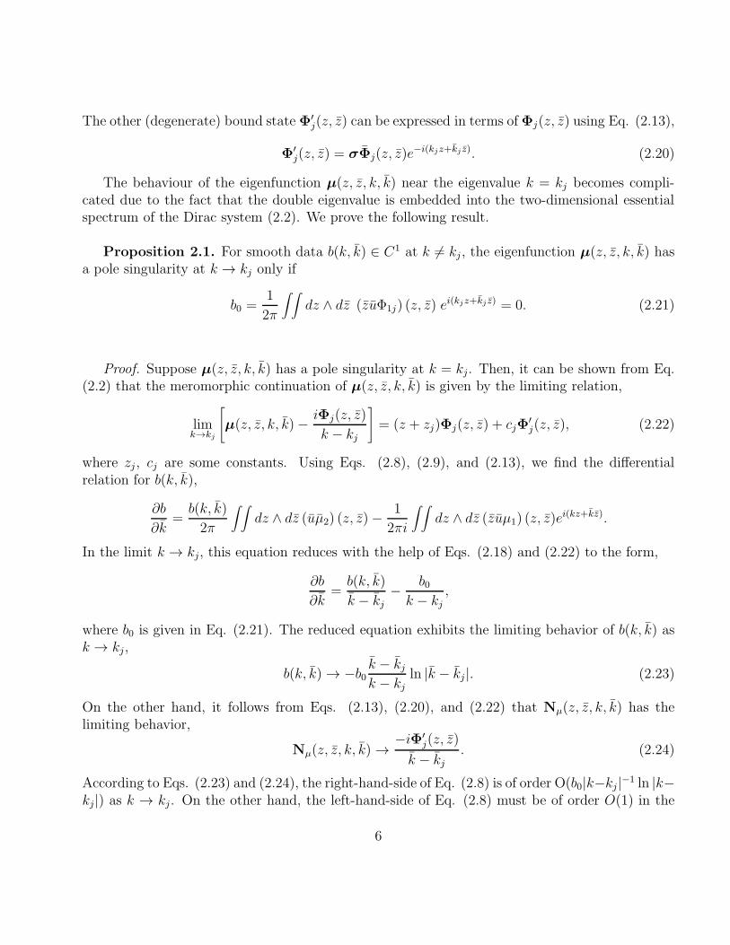
The other (degenerate) bound state Φ′j(z, z) can be expressed in terms ofΦj(z, z) using Eq. (2.13),

Φ′j(z, z) = σΦj(z, z)e

−i(kjz+kj z). (2.20)

The behaviour of the eigenfunction µ(z, z, k, k) near the eigenvalue k = kj becomes compli-cated due to the fact that the double eigenvalue is embedded into the two-dimensional essentialspectrum of the Dirac system (2.2). We prove the following result.

Proposition 2.1. For smooth data b(k, k) ∈ C1 at k 6= kj , the eigenfunction µ(z, z, k, k) hasa pole singularity at k → kj only if

b0 =1

2π

∫ ∫

dz ∧ dz (zuΦ1j) (z, z) ei(kjz+kj z) = 0. (2.21)

Proof. Suppose µ(z, z, k, k) has a pole singularity at k = kj. Then, it can be shown from Eq.(2.2) that the meromorphic continuation of µ(z, z, k, k) is given by the limiting relation,

limk→kj

[

µ(z, z, k, k)− iΦj(z, z)

k − kj

]

= (z + zj)Φj(z, z) + cjΦ′j(z, z), (2.22)

where zj , cj are some constants. Using Eqs. (2.8), (2.9), and (2.13), we find the differentialrelation for b(k, k),

∂b

∂k=

b(k, k)

2π

∫ ∫

dz ∧ dz (uµ2) (z, z)−1

2πi

∫ ∫

dz ∧ dz (zuµ1) (z, z)ei(kz+kz).

In the limit k → kj, this equation reduces with the help of Eqs. (2.18) and (2.22) to the form,

∂b

∂k=

b(k, k)

k − kj− b0

k − kj,

where b0 is given in Eq. (2.21). The reduced equation exhibits the limiting behavior of b(k, k) ask → kj,

b(k, k) → −b0k − kjk − kj

ln |k − kj |. (2.23)

On the other hand, it follows from Eqs. (2.13), (2.20), and (2.22) that Nµ(z, z, k, k) has thelimiting behavior,

Nµ(z, z, k, k) →−iΦ′

j(z, z)

k − kj. (2.24)

According to Eqs. (2.23) and (2.24), the right-hand-side of Eq. (2.8) is of order O(b0|k−kj|−1 ln |k−kj|) as k → kj. On the other hand, the left-hand-side of Eq. (2.8) must be of order O(1) in the

6

limit k → kj according to Eq. (2.22). Therefore, the eigenfunction µ(z, z, k, k) has a pole atk = kj only if the constraint b0 = 0 holds. ✷

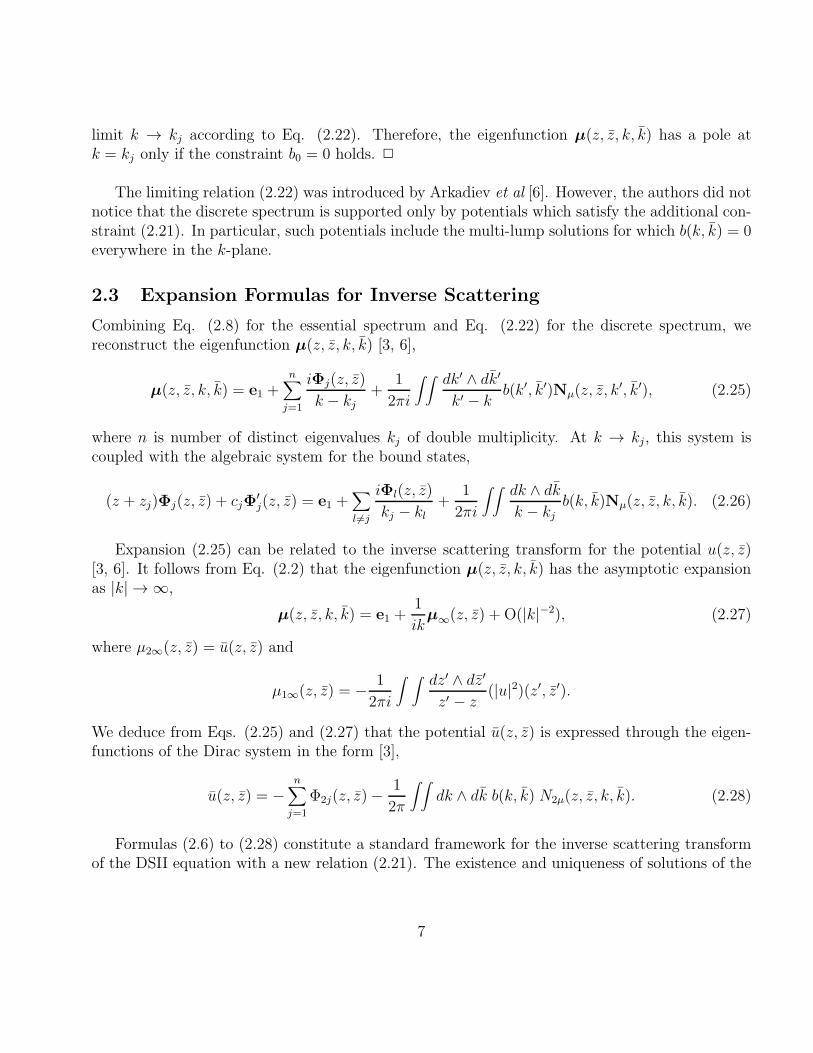
The limiting relation (2.22) was introduced by Arkadiev et al [6]. However, the authors did notnotice that the discrete spectrum is supported only by potentials which satisfy the additional con-straint (2.21). In particular, such potentials include the multi-lump solutions for which b(k, k) = 0everywhere in the k-plane.

2.3 Expansion Formulas for Inverse Scattering

Combining Eq. (2.8) for the essential spectrum and Eq. (2.22) for the discrete spectrum, wereconstruct the eigenfunction µ(z, z, k, k) [3, 6],

µ(z, z, k, k) = e1 +n∑

j=1

iΦj(z, z)

k − kj+

1

2πi

∫ ∫ dk′ ∧ dk′

k′ − kb(k′, k′)Nµ(z, z, k

′, k′), (2.25)

where n is number of distinct eigenvalues kj of double multiplicity. At k → kj, this system iscoupled with the algebraic system for the bound states,

(z + zj)Φj(z, z) + cjΦ′j(z, z) = e1 +

∑

l 6=j

iΦl(z, z)

kj − kl+

1

2πi

∫ ∫

dk ∧ dk

k − kjb(k, k)Nµ(z, z, k, k). (2.26)

Expansion (2.25) can be related to the inverse scattering transform for the potential u(z, z)[3, 6]. It follows from Eq. (2.2) that the eigenfunction µ(z, z, k, k) has the asymptotic expansionas |k| → ∞,

µ(z, z, k, k) = e1 +1

ikµ∞(z, z) + O(|k|−2), (2.27)

where µ2∞(z, z) = u(z, z) and

µ1∞(z, z) = − 1

2πi

∫ ∫

dz′ ∧ dz′

z′ − z(|u|2)(z′, z′).

We deduce from Eqs. (2.25) and (2.27) that the potential u(z, z) is expressed through the eigen-functions of the Dirac system in the form [3],

u(z, z) = −n∑

j=1

Φ2j(z, z)−1

2π

∫ ∫

dk ∧ dk b(k, k) N2µ(z, z, k, k). (2.28)

Formulas (2.6) to (2.28) constitute a standard framework for the inverse scattering transformof the DSII equation with a new relation (2.21). The existence and uniqueness of solutions of the

7

Fredholm integral equations (2.6) and (2.7) and the ∂ problem (2.8) and (2.25) were proved in [4]and [5] under the small-norm assumption for the potential u(x, y),

(

sup(x,y)∈R2

|u|(x, y))

(∫ ∫

|u(x, y)|dxdy)

<π

8.

In this case n = 0 and b(k, k) 6= 0. The nonlinear two-dimensional Fourier transform associatedto this scheme was discussed in Examples 8-10 of Chapter 7.7 of Ref. [17]. Indeed, the connectionformula (2.28) implies that there is a scalar spectral decomposition of u(z, z) throughN2µ(z, z, k, k)for n = 0. In order to close the decomposition, one could use Eqs. (2.9) and (2.13) to construct a“completeness relation” for the expansion of δ(z′ − z) in the form,

δ(z′ − z) = − 1

2π2i

∫ ∫

dk ∧ dkN2µ(z′, z′, k, k)N2µ(z, z, k, k).

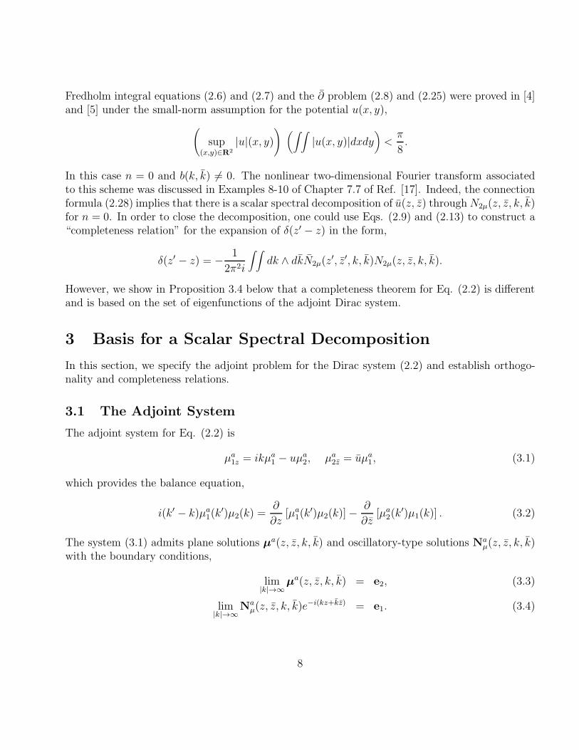
However, we show in Proposition 3.4 below that a completeness theorem for Eq. (2.2) is differentand is based on the set of eigenfunctions of the adjoint Dirac system.

3 Basis for a Scalar Spectral Decomposition

In this section, we specify the adjoint problem for the Dirac system (2.2) and establish orthogo-nality and completeness relations.

3.1 The Adjoint System

The adjoint system for Eq. (2.2) is

µa1z = ikµa

1 − uµa2, µa

2z = uµa1, (3.1)

which provides the balance equation,

i(k′ − k)µa1(k

′)µ2(k) =∂

∂z[µa

1(k′)µ2(k)]−

∂

∂z[µa

2(k′)µ1(k)] . (3.2)

The system (3.1) admits plane solutions µa(z, z, k, k) and oscillatory-type solutions Naµ(z, z, k, k)

with the boundary conditions,

lim|k|→∞

µa(z, z, k, k) = e2, (3.3)

lim|k|→∞

Naµ(z, z, k, k)e

−i(kz+kz) = e1. (3.4)

8

The adjoint eigenfunctions Naµ(z, z, k, k) can be expressed through the Green functions,

Na1µ(z, z) = ei(kz+kz) − 1

2πi

∫ ∫

dz′ ∧ dz′

z′ − z(uNa

2µ)(z′, z′)eik(z−z′)+ik(z−z′), (3.5)

Na2µ(z, z) =

1

2πi

∫ ∫ dz′ ∧ dz′

z′ − z(uNa

1µ)(z′, z′). (3.6)

They are related to the adjoint eigenfunctions µa(z, z, k, k) by the formula,

Naµ(z, z, k, k) = −σµ

a(z, z, k, k)ei(kz+kz). (3.7)

Using this representation, we prove the following result.

Lemma 3.1. The spectral data b(k, k) is expressed in terms of the adjoint eigenfunctions as

b(k, k) =1

2π

∫ ∫

dz ∧ dz(uNa1µ)(z, z). (3.8)

Proof. Multiplying Eq. (3.5) by uµ1(k), integrating over dz ∧ dz and using Eq. (2.7), weexpress b(k, k) defined in Eq. (2.9) in the form,

b(k, k) =1

2π

∫ ∫

dz ∧ dz[

uµ1(k)Na1µ(k)− uµ2(k)N

a2µ(k)

]

. (3.9)

On the other hand, multiplying Eq. (2.6) by uNa1µ(k), integrating over dz ∧ dz, and using Eqs.

(3.6) and (3.9), we get Eq. (3.8). ✷

Suppose now that k = kj is an isolated double eigenvalue of Eq. (2.2) with the bound statesΦj(z, z) and Φ′

j(z, z) given by Eqs. (2.15) – (2.20). Suppose also that k = kaj is an eigenvalue of

the adjoint system (3.1) with the adjoint bound states Φaj (z, z) and Φa′

j (z, z).

Lemma 3.2. If kj is a double eigenvalue of the Dirac system (2.2), then kj is also a doubleeigenvalue of the adjoint system (3.1).

Proof. We use Eq. (3.2) with µ = Φj(z, z) and µa = Φa

j (z, z) at k = kj and k′ = kaj and

integrate over dz ∧ dz with the help of Eq. (A.3) of Appendix A. The contour contribution of theintegral vanishes due to the boundary conditions (2.17) and (3.12) and the resulting expression is

(kaj − kj)

∫ ∫

dz ∧ dz (Φa1jΦ2j)(z, z) = 0.

The relation kaj = kj follows from this formula if the integral is non-zero at ka

j = kj (which isproved below in Eq. (3.22)). The other possibility is when ka

j 6= kj but Φa1j is orthogonal to Φ2j .

We do not consider such a non-generic situation. The other bound state Φa′j at ka

j = kj can be

9

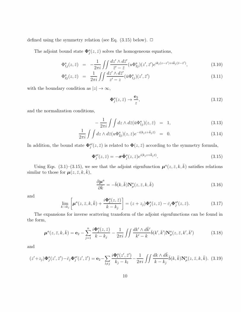
defined using the symmetry relation (see Eq. (3.15) below). ✷

The adjoint bound state Φaj (z, z) solves the homogeneous equations,

Φa1j(z, z) = − 1

2πi

∫ ∫ dz′ ∧ dz′

z′ − z(uΦa

2j)(z′, z′)eikj(z−z′)+ikj(z−z′), (3.10)

Φa2j(z, z) =

1

2πi

∫ ∫

dz′ ∧ dz′

z′ − z(uΦa

1j)(z′, z′) (3.11)

with the boundary condition as |z| → ∞,

Φaj (z, z) →

e2

z, (3.12)

and the normalization conditions,

− 1

2πi

∫ ∫

dz ∧ dz(uΦa1j)(z, z) = 1, (3.13)

1

2πi

∫ ∫

dz ∧ dz(uΦa2j)(z, z)e

−i(kjz+kj z) = 0. (3.14)

In addition, the bound state Φa′j (z, z) is related to Φ(z, z) according to the symmetry formula,

Φa′j (z, z) = −σΦa

j (z, z)ei(kjz+kj z). (3.15)

Using Eqs. (3.1)–(3.15), we see that the adjoint eigenfunction µa(z, z, k, k) satisfies relations

similar to those for µ(z, z, k, k),

∂µa

∂k= −b(k, k)Na

µ(z, z, k, k) (3.16)

and

limk→kj

[

µa(z, z, k, k) +

iΦaj (z, z)

k − kj

]

= (z + zj)Φaj (z, z)− cjΦ

a′j (z, z). (3.17)

The expansions for inverse scattering transform of the adjoint eigenfunctions can be found inthe form,

µa(z, z, k, k) = e2 −

n∑

j=1

iΦaj (z, z)

k − kj− 1

2πi

∫ ∫ dk′ ∧ dk′

k′ − kb(k′, k′)Na

µ(z, z, k′, k′) (3.18)

and

(z′+zj)Φaj (z

′, z′)−cjΦa′j (z

′, z′) = e2−∑

l 6=j

iΦal (z

′, z′)

kj − kl− 1

2πi

∫ ∫ dk ∧ dk

k − kjb(k, k)Na

µ(z, z, k, k). (3.19)

10

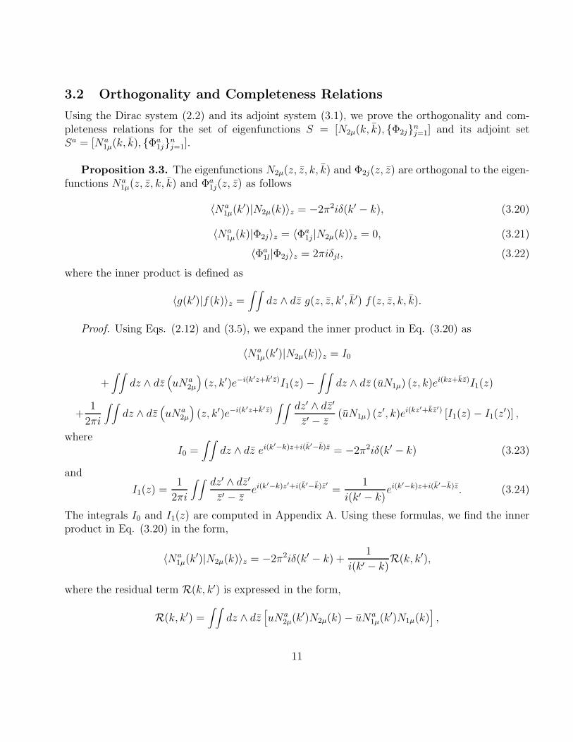
3.2 Orthogonality and Completeness Relations

Using the Dirac system (2.2) and its adjoint system (3.1), we prove the orthogonality and com-pleteness relations for the set of eigenfunctions S = [N2µ(k, k), {Φ2j}nj=1] and its adjoint setSa = [Na

1µ(k, k), {Φa1j}nj=1].

Proposition 3.3. The eigenfunctions N2µ(z, z, k, k) and Φ2j(z, z) are orthogonal to the eigen-functions Na

1µ(z, z, k, k) and Φa1j(z, z) as follows

〈Na1µ(k

′)|N2µ(k)〉z = −2π2iδ(k′ − k), (3.20)

〈Na1µ(k)|Φ2j〉z = 〈Φa

1j |N2µ(k)〉z = 0, (3.21)

〈Φa1l|Φ2j〉z = 2πiδjl, (3.22)

where the inner product is defined as

〈g(k′)|f(k)〉z =∫ ∫

dz ∧ dz g(z, z, k′, k′) f(z, z, k, k).

Proof. Using Eqs. (2.12) and (3.5), we expand the inner product in Eq. (3.20) as

〈Na1µ(k

′)|N2µ(k)〉z = I0

+∫ ∫

dz ∧ dz(

uNa2µ

)

(z, k′)e−i(k′z+k′z)I1(z)−∫ ∫

dz ∧ dz (uN1µ) (z, k)ei(kz+kz)I1(z)

+1

2πi

∫ ∫

dz ∧ dz(

uNa2µ

)

(z, k′)e−i(k′z+k′z)∫ ∫

dz′ ∧ dz′

z′ − z(uN1µ) (z

′, k)ei(kz′+kz′) [I1(z)− I1(z

′)] ,

whereI0 =

∫ ∫

dz ∧ dz ei(k′−k)z+i(k′−k)z = −2π2iδ(k′ − k) (3.23)

and

I1(z) =1

2πi

∫ ∫

dz′ ∧ dz′

z′ − zei(k

′−k)z′+i(k′−k)z′ =1

i(k′ − k)ei(k

′−k)z+i(k′−k)z. (3.24)

The integrals I0 and I1(z) are computed in Appendix A. Using these formulas, we find the innerproduct in Eq. (3.20) in the form,

〈Na1µ(k

′)|N2µ(k)〉z = −2π2iδ(k′ − k) +1

i(k′ − k)R(k, k′),

where the residual term R(k, k′) is expressed in the form,

R(k, k′) =∫ ∫

dz ∧ dz[

uNa2µ(k

′)N2µ(k)− uNa1µ(k

′)N1µ(k)]

,

11

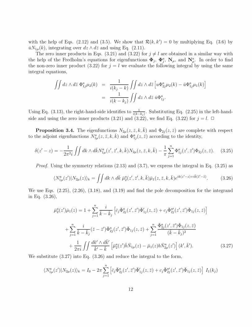
with the help of Eqs. (2.12) and (3.5). We show that R(k, k′) = 0 by multiplying Eq. (3.6) byuN1µ(k), integrating over dz ∧ dz and using Eq. (2.11).

The zero inner products in Eqs. (3.21) and (3.22) for j 6= l are obtained in a similar way withthe help of the Fredholm’s equations for eigenfunctions Φj, Φ

aj , Nµ, and Na

µ. In order to findthe non-zero inner product (3.22) for j = l we evaluate the following integral by using the sameintegral equations,

∫ ∫

dz ∧ dz Φa1jµ2(k) =

1

i(kj − k)

∫ ∫

dz ∧ dz[

uΦa2jµ2(k)− uΦa

1jµ1(k)]

=1

i(k − kj)

∫ ∫

dz ∧ dz uΦa1j .

Using Eq. (3.13), the right-hand-side identifies to 1i(k−kj)

. Substituting Eq. (2.25) in the left-hand-

side and using the zero inner products (3.21) and (3.22), we find Eq. (3.22) for j = l. ✷

Proposition 3.4. The eigenfunctions N2µ(z, z, k, k) and Φ2j(z, z) are complete with respectto the adjoint eigenfunctions Na

1µ(z, z, k, k) and Φa1j(z, z) according to the identity,

δ(z′ − z) = − 1

2π2i

∫ ∫

dk ∧ dkNa1µ(z

′, z′, k, k)N2µ(z, z, k, k)−1

π

n∑

j=1

Φa1j(z

′, z′)Φ2j(z, z). (3.25)

Proof. Using the symmetry relations (2.13) and (3.7), we express the integral in Eq. (3.25) as

〈Na1µ(z

′)|N2µ(z)〉k =∫ ∫

dk ∧ dk µa2(z

′, z′, k, k)µ1(z, z, k, k)eik(z′−z)+ik(z′−z). (3.26)

We use Eqs. (2.25), (2.26), (3.18), and (3.19) and find the pole decomposition for the integrandin Eq. (3.26),

µa2(z

′)µ1(z) = 1 +n∑

j=1

i

k − kj

[

cjΦa2j(z

′, z′)Φ′1j(z, z) + cjΦ

a′2j(z

′, z′)Φ1j(z, z)]

+n∑

j=1

i

k − kj(z − z′)Φa

2j(z′, z′)Φ1j(z, z) +

n∑

j=1

Φa2j(z

′, z′)Φ1j(z, z)

(k − kj)2

+1

2πi

∫ ∫

dk′ ∧ dk′

k′ − k

[

µa2(z

′)bN1µ(z)− µ1(z)bNa2µ(z

′)]

(k′, k′). (3.27)

We substitute (3.27) into Eq. (3.26) and reduce the integral to the form,

〈Na1µ(z

′)|N2µ(z)〉k = I0 − 2πn∑

j=1

[

cjΦa2j(z

′, z′)Φ′1j(z, z) + cjΦ

a′2j(z

′, z′)Φ1j(z, z)]

I1(kj)

12

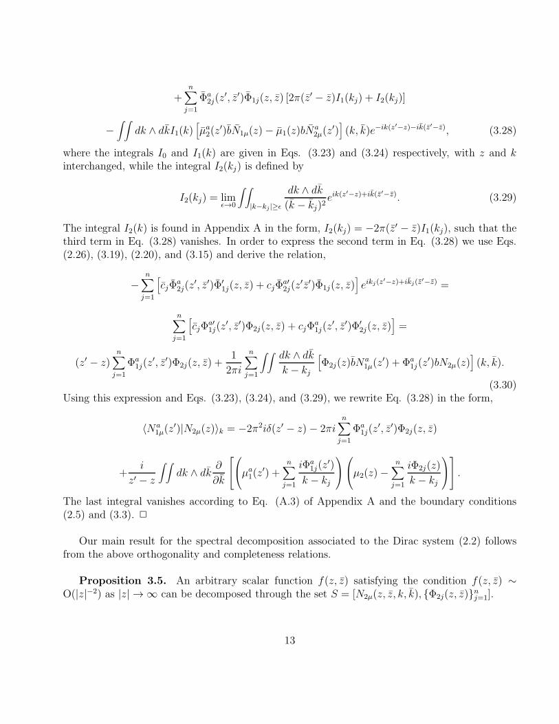
+n∑

j=1

Φa2j(z

′, z′)Φ1j(z, z) [2π(z′ − z)I1(kj) + I2(kj)]

−∫ ∫

dk ∧ dkI1(k)[

µa2(z

′)bN1µ(z)− µ1(z)bNa2µ(z

′)]

(k, k)e−ik(z′−z)−ik(z′−z), (3.28)

where the integrals I0 and I1(k) are given in Eqs. (3.23) and (3.24) respectively, with z and kinterchanged, while the integral I2(kj) is defined by

I2(kj) = limǫ→0

∫ ∫

|k−kj |≥ǫ

dk ∧ dk

(k − kj)2eik(z

′−z)+ik(z′−z). (3.29)

The integral I2(k) is found in Appendix A in the form, I2(kj) = −2π(z′ − z)I1(kj), such that thethird term in Eq. (3.28) vanishes. In order to express the second term in Eq. (3.28) we use Eqs.(2.26), (3.19), (2.20), and (3.15) and derive the relation,

−n∑

j=1

[

cjΦa2j(z

′, z′)Φ′1j(z, z) + cjΦ

a′2j(z

′z′)Φ1j(z, z)]

eikj(z′−z)+ikj(z′−z) =

n∑

j=1

[

cjΦa′1j(z

′, z′)Φ2j(z, z) + cjΦa1j(z

′, z′)Φ′2j(z, z)

]

=

(z′ − z)n∑

j=1

Φa1j(z

′, z′)Φ2j(z, z) +1

2πi

n∑

j=1

∫ ∫

dk ∧ dk

k − kj

[

Φ2j(z)bNa1µ(z

′) + Φa1j(z

′)bN2µ(z)]

(k, k).

(3.30)Using this expression and Eqs. (3.23), (3.24), and (3.29), we rewrite Eq. (3.28) in the form,

〈Na1µ(z

′)|N2µ(z)〉k = −2π2iδ(z′ − z)− 2πin∑

j=1

Φa1j(z

′, z′)Φ2j(z, z)

+i

z′ − z

∫ ∫

dk ∧ dk∂

∂k

µa1(z

′) +n∑

j=1

iΦa1j(z

′)

k − kj

µ2(z)−n∑

j=1

iΦ2j(z)

k − kj

.

The last integral vanishes according to Eq. (A.3) of Appendix A and the boundary conditions(2.5) and (3.3). ✷

Our main result for the spectral decomposition associated to the Dirac system (2.2) followsfrom the above orthogonality and completeness relations.

Proposition 3.5. An arbitrary scalar function f(z, z) satisfying the condition f(z, z) ∼O(|z|−2) as |z| → ∞ can be decomposed through the set S = [N2µ(z, z, k, k), {Φ2j(z, z)}nj=1].

13

Proof. The spectral decomposition is defined through the orthogonality relations (3.20)–(3.22)as

f(z, z) =∫ ∫

dk ∧ dkα(k, k)N2µ(z, z, k, k) +n∑

j=1

αjΦ2j(z, z), (3.31)

where

α(k, k) = − 1

4π2〈Na

1µ(k)|f〉z, αj =1

2πi〈Φa

1j |f〉z. (3.32)

Provided the condition on f(z, z) is satisfied, we interchange integration with respect to dz ∧ dzand dk ∧ dk and use the completeness formula (3.25). ✷

The spectral decomposition presented here is different from that of Kiselev [10, 11]. In thelatter approach, the function f(z, z) is spanned by squared eigenfunctions of the original problem(1.2) defined according to oscillatory-type behaviour at infinity. In our approach, we transformedthe system (1.2) to the form (2.2) and defined the oscillatory-type eigenfunctions according to thesingle eigenfunctions Nµ(z, z, k, k). We also notice that the (degenerate) bound states Φ′

j(z, z)are not relevant for the spectral decomposition, although they appear implicitly through themeromorphic contributions of the eigenfunctions Nµ(z, z, k, k) at k = kj (see Section 4).

4 Perturbation Theory for a Single Lump

We use the scalar spectral decomposition based on Eq. (3.31) and develop a perturbation theoryfor multi-lump solutions of the DSII equation. We present formulas in the case of a single lump(n = 1), the case of multi-lump potentials can be obtained by summing along the indices j, loccuring in the expressions below.

The single-lump potential u(z, z) has the form [6],

u(z, z) =cj

|z + zj |2 + |cj|2ei(kjz+kj z), (4.1)

where cj , zj are complex parameters. The associated bound states follow from Eqs. (2.26) and(3.19) as

Φj(z, z) =1

|z + zj|2 + |cj|2[

z + zj−cje

−i(kjz+kj z)

]

, (4.2)

Φaj (z, z) =

1

|z + zj|2 + |cj|2[

cjei(kjz+kj z)

z + zj

]

. (4.3)

We first consider a general perturbation to the single lump subject to the localization condition,∆u ∼ O(|z|−2) as |z| → ∞. We then derive explicit formulas for a special form of the perturbationterm ∆u(z, z).

14

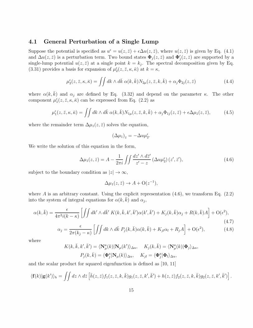
4.1 General Perturbation of a Single Lump

Suppose the potential is specified as uǫ = u(z, z) + ǫ∆u(z, z), where u(z, z) is given by Eq. (4.1)and ∆u(z, z) is a perturbation term. Two bound states Φj(z, z) and Φ′

j(z, z) are supported by asingle-lump potential u(z, z) at a single point k = kj . The spectral decomposition given by Eq.(3.31) provides a basis for expansion of µǫ

2(z, z, κ, κ) at k = κ,

µǫ2(z, z, κ, κ) =

∫ ∫

dk ∧ dk α(k, k)N2µ(z, z, k, k) + αjΦ2j(z, z) (4.4)

where α(k, k) and αj are defined by Eq. (3.32) and depend on the parameter κ. The othercomponent µǫ

1(z, z, κ, κ) can be expressed from Eq. (2.2) as

µǫ1(z, z, κ, κ) =

∫ ∫

dk ∧ dk α(k, k)N1µ(z, z, k, k) + αjΦ1j(z, z) + ǫ∆µ1(z, z), (4.5)

where the remainder term ∆µ1(z, z) solves the equation,

(∆µ1)z = −∆uµǫ2.

We write the solution of this equation in the form,

∆µ1(z, z) = A− 1

2πi

∫ ∫

dz′ ∧ dz′

z′ − z(∆uµǫ

2) (z′, z′), (4.6)

subject to the boundary condition as |z| → ∞,

∆µ1(z, z) → A+O(z−1),

where A is an arbitrary constant. Using the explicit representation (4.6), we transform Eq. (2.2)into the system of integral equations for α(k, k) and αj ,

α(k, k) =ǫ

4π2i(k − κ)

[∫ ∫

dk′ ∧ dk′ K(k, k, k′, k′)α(k′, k′) +Kj(k, k)αj +R(k, k)A]

+O(ǫ2),

(4.7)

αj =ǫ

2π(kj − κ)

[∫ ∫

dk ∧ dk Pj(k, k)α(k, k) +Kjlαl +RjA]

+O(ǫ2), (4.8)

whereK(k, k, k′, k′) = 〈Na

µ(k)|Nµ(k′)〉∆u, Kj(k, k) = 〈Na

µ(k)|Φj〉∆u,

Pj(k, k) = 〈Φaj |Nµ(k)〉∆u, Kjl = 〈Φa

j |Φl〉∆u,

and the scalar product for squared eigenfunction is defined as [10, 11]

〈f(k)|g(k′)〉h =∫ ∫

dz ∧ dz[

h(z, z)f1(z, z, k, k)g1(z, z, k′, k′) + h(z, z)f2(z, z, k, k)g2(z, z, k

′, k′)]

.

15

The non-homogeneous terms R(k, k) and Rj can be computed exactly as

R(k, k) =∫ ∫

dz ∧ dz(

uNa1µ

)

(z, z) = 2πb(k, k),

Rj =∫ ∫

dz ∧ dz(

uΦa1j

)

(z, z) = −2πi,

where b(k, k) = 0 if n 6= 0. We solve the system of equations (4.7) and (4.8) asymptotically forκ = kj + ǫ∆κ and ∆κ ∼ O(1). The leading order behaviour of the integral kernels follows fromthe asymptotic representation (2.24) as k → kj ,

K(k, k, k′, k′) → Kjj

(k − kj)(k′ − kj), Kj(k, k) →

iPjj

k − kj, Pj(k, k) →

iPjj

k − kj, (4.9)

whereKjj = 〈Φa′

j |Φ′j〉∆u, Pjj = 〈Φa′

j |Φj〉∆u, Pjj = −〈Φaj |Φ′

j〉∆u. (4.10)

Here we have used the symmetry constraints (2.20) and (3.15). The leading order of α(k, k) ask → kj follows from Eq. (4.7) as

α(k, k) → − ǫ∆κβj

2π(k − κ)(k − kj),

where βj is not yet defined. We use Eq. (A.4) of Appendix A to compute the integral term,

∫ ∫ dk ∧ dk

(k − κ)(k − kj)2=

2πi

kj − κ,

and reduce the system of integral equations (4.7) and (4.8) to an algebraic system as k → kj ,

− 2π∆καj = Kjjαj − Pjjβj − 2πiA, (4.11)

2π∆κβj = −Pjjαj − Kjjβj . (4.12)

If Pjj 6= 0, the determinant of the above system is strictly positive. Therefore, homogeneoussolutions at A = 0 (bound states) are absent for ǫ 6= 0. This result indicates that the doubleeigenvalue at k = kj disappears under a generic perturbation of the potential u(z, z) with Pjj 6= 0(see also Ref. [8]).

For A 6= 0, we find inhomogeneous solutions of Eqs. (4.11) and (4.12),

αj =2πiA

(

Kjj + 2π∆κ)

|Kjj + 2π∆κ|2 + |Pjj|2, βj =

−2πiAPjj

|Kjj + 2π∆κ|2 + |Pjj|2. (4.13)

16

The eigenfunction µǫ(z, z, κ, κ) given by Eqs. (4.4) and (4.5) satisfies the boundary condition

(2.5) if A = ǫ−1 and has the following asymptotic representation,

µǫ(z, z, κ, κ) = e1 +

2πi[

2π(κ− kj) + ǫKjj

]

Φj(z, z)

|2π(κ− kj) + ǫKjj |2 + |ǫPjj|2− 2πiǫPjjΦ

′j(z, z)

|2π(κ− kj) + ǫKjj|2 + |ǫPjj|2+ ∆µ

ǫ(z, z), (4.14)

where the term ∆µǫ(z, z) is not singular in the limit ǫ → 0 and κ → kj .

In the limit ǫ → 0, κ 6= kj, we find a meromorphic expansion for µǫ(z, z, κ, κ) as

µǫ(z, z, κ, κ) = e1 +

iΦj(z, z)

κ− kj+ ǫ

[

KjjΦj(z, z)

2πi(κ− kj)2+

PjjΦ′j(z, z)

2πi|κ− kj |2]

+O(ǫ2). (4.15)

It is clear that the double pole can be incorporated by shifting the eigenvalue kj to

kǫj = kj −

ǫKjj

2π.

The other double-pole term in the expansion (4.15) has a non-analytic behaviour in the k-planeand leads to the appearance of the spectral data bǫ(κ, κ) = ǫ∆b(κ, κ) which measures the departureof µǫ(z, z, κ, κ) from analyticity according to Eq. (2.8). We find from Eqs. (2.9) and (4.15) thatthe spectral data ∆b(κ, κ) has the following singular behaviour as κ → kj

∆b(κ, κ) → −Pjj

2π|κ− kj |2. (4.16)

Thus, if Pjj 6= 0 the analyticity of µǫ(z, z, κ, κ) is destroyed and the lump disappears. This

conclusion as well as the analytical solution (4.13) agree with the results of Gadyl’shin and Kiselev[8, 9] where the transformation of a single lump into decaying wave packet was also studied.

In the other limit ǫ 6= 0 and κ → kǫj we find another expansion from Eq. (4.14),

µǫ(z, z, κ, κ) = e1 −

2πi

ǫPjj

Φ′j(z, z) + O(κ− kǫ

j). (4.17)

We conclude that the eigenfunction µǫ(z, z, κ, κ) is now free of pole singularities [8, 9]. We sum-

marize the main result in the form of a proposition.

Proposition 4.1. Suppose u(z, z) is given by Eq. (4.1) and ∆u(z, z) satisfies the constraint,

Pjj = 〈Φa′j |Φj〉∆u 6= 0.

Then, the potential uǫ = u(z, z) + ǫ∆u(z, z) does not support embedded eigenvalues of the Diracsystem (2.2) for ǫ 6= 0.

17

4.2 Explicit Solution for a Particular Perturbation

Here we specify cj = ceiθ, where c and θ are real, and consider a particular perturbation ∆u(z, z)to the lump u(z, z) (4.1) in the form,

∆u(z, z) = Q(z, z)ei(kjz+kj z+θ),

where Q(z, z) is a real function. Using Eqs. (4.10), (4.2), and (4.3), we find explicitly the matrixelements Kjj and Pjj,

Kjj =∫ ∫

dz ∧ dzc(z + zj)[Q(z, z)− Q(z, z)]

[|z + zj |2 + c2]2= 0,

Pjj =∫ ∫

dz ∧ dz|z + zj |2Q(z, z) + c2Q(z, z)

[|z + zj |2 + c2]2=

1

2c

∫ ∫

dz ∧ dz (u∆u+ u∆u) .

The element Pjj can be seen as a correction to the field energy,

N =i

2

∫ ∫

dz ∧ dz|uǫ|2(z, z) = N0 + iǫcPjj +O(ǫ2),

where N0 = π is the energy of the single lump solution (independent of the lump parameters kjand cj). Thus, a perturbation which leads to the destruction of a single lump, that is with Pjj 6= 0,changes necessarily the value for the lump energy N0.

5 Concluding Remarks

The main result of our paper is the prediction of structural instability of multi-lump potentialsin the Dirac system associated to the DSII equation. The multi-lump potentials correspond toeigenvalues embedded into a two-dimensional continuous spectrum with the spectral data b(k, k)satisfying the additional constraint (2.21). In this case, there is no interaction between lumpsand continuous radiation. However, a generic initial perturbation induces coupling between thelumps and radiation and, as a result of their interaction, the embedded eigenvalues disappear.This result indicates that the localized multi-lump solutions decay into continuous wave packetsin the nonlinear dynamics of the DSII equation (see also Refs. [8, 9]).

This scenario is different from the two types of bifurcations of embedded eigenvalues discussedin our previous paper [14]. The type I bifurcation arises from the edge of the essential spectrumwhen the limiting bounded (non-localized) eigenfunction is transformed into a localized boundstate. The type II bifurcation occurs when an embedded eigenvalue splits off the essential spec-trum. Both situations persist in the spectral plane when the essential spectrum is one-dimensionaland covers either a half-axis or the whole axis. However, in the case of the DSII equation, the es-sential spectrum is the whole spectral plane and embedded eigenvalue can not split off the essentialspectrum. As a result, they disappear due to their structural instability.

18

Acknowledgements

We benefited from stimulating discussions with M. Ablowitz, A. Fokas, D. Kaup, O. Kiselev, andA. Yurov. D.P. acknowledges support from a NATO fellowship provided by NSERC and C.S.acknowledges support from NSERC Operating grant OGP0046179.

Appendix A. Formulas of the ∂-analysis

Here we reproduce some formulas of the complex ∂-analysis [17] to compute the integrals I0, I1(z)and I2(z) defined in Eqs. (3.23), (3.24), and (3.29). We define the complex integration in thez-plane by

∫ ∫

dz ∧ dzf(z, z) = −∫ ∫

dz ∧ dzf(z, z),

where dz ∧ dz = −2idxdy. The complex δ(z) distribution is defined by∫ ∫

dz ∧ dzf(z)δ(z − z0) = −2if(z0), (A.1)

where δ(z) = δ(x)δ(y). In particular, the δ-distribution appears in the ∂-analysis according to therelation [17],

∂

∂z

[

1

z − z0

]

= πδ(z − z0). (A.2)

Computing the integral I0, we get the formula,

I0 =∫ ∫

dz ∧ dzeikz+ikz = −2i∫ ∫

dxdye2iRe(k)x−2iIm(k)y = −2π2iδ(k),

which proves the identity (3.23).Using the Green’s theorem [17], one has the integration identity,

∫ ∫

Ddz ∧ dz

(

∂f1∂z

− ∂f2∂z

)

=∫

C(f1dz + f2dz) , (A.3)

where D is a domain of the complex plane and C its boundary. The generalized Cauchy’s formulahas the form [17],

f(z, z) =1

2πi

∫

C

f(z′, z′)dz′

z′ − z+

1

2πi

∫ ∫

D

dz′ ∧ dz′

z′ − z

∂f

∂z′, (A.4)

or, equivalently,

f(z, z) = − 1

2πi

∫

C

f(z′, z′)dz′

z′ − z+

1

2πi

∫ ∫

D

dz′ ∧ dz′

z′ − z

∂f

∂z′. (A.5)

In order to find the integral I1(z) we use Eq. (A.5) with

f(z, z) =1

ikei(kz+kz), k 6= 0

19

and choose the domain D to be a large ball of radius R (see Eq. (2.14)). The boundary valueintegral vanishes since

limR→∞

∫

|z|=R

dz

zei(kz+kz) = −2πi lim

R→∞J0(2|k|R) = 0, (A.6)

where J0(z) is the Bessel function. Equation (A.5) for the function f(z, z) then reduces to Eq.(3.24).

In order to compute the integral I2(z0), we apply Eq. (A.3) with f1 = 0 and

f2(z, z) =1

z − z0ei(kz+kz).

The domain D is chosen as above. The boundary value integral vanishes again,

limR→∞

∫

|z|=R

dz

zei(kz+kz) = −2πi lim

R→∞J−2(2|k|R) = 0, (A.7)

where J−2(z) is the Bessel function. Equation (A.3) for the function f2(z, z) reduces to Eq. (3.29).

References

[1] A. Davey and K. Stewartson, On three-dimensional packets of surface waves, Proc. R. Soc.Lond. A 388, 101–110 (1974).

[2] M.J. Ablowitz and P.A. Clarkson, Solitons, nonlinear evolution equations and inverse scat-tering Cambridge University Press, Cambridge (1991).

[3] A.S. Fokas and M.J. Ablowitz, On the inverse scattering transform of multidimensional non-linear equations related to first-order systems in the plane, J. Math. Phys. 25, 2494–2505(1984).

[4] R. Beals and R.R. Coifman, The D-bar approach to inverse scattering and nonlinear evolu-tions, Physica D 18, 242–249 (1986).

[5] A.S. Fokas and L.Y. Sung, On the solvability of the N-Wave, Davey–Stewartson andKadomtsev–Petviashvili equations, Inverse Problems 8, 673–708 (1992).

[6] V.A. Arkadiev, A.K. Pogrebkov, and M.C. Polivanov, Inverse scattering transform methodand soliton solutions for Davey–Stewartson II equation, Physica D 36, 189–197 (1989).

[7] V.A. Arkadiev, A.K. Pogrebkov, and M.C. Polivanov, Closed string-like solutions of theDavey–Stewartson equation, Inverse Problems 5, L1-L6 (1989).

20

[8] R.R. Gadyl’shin and O.M. Kiselev, On solitonless structure of the scattering data for a per-turbed two-dimensional soliton of the Davey–Stewartson equation, Teor. Mat. Phys. 161,200–208 (1996).

[9] R.R. Gadyl’shin and O.M. Kiselev, Structural instability of soliton for the Davey–StewartsonII equation, Teor. Mat. Fiz. 118, 354–361 (1999).

[10] O.M. Kiselev, Basic functions associated with a two-dimensional Dirac system, Funct. Anal.Appl. 32, 56–59 (1998).

[11] O.M. Kiselev, Perturbation theory for the Dirac equation in two-dimensional space, J. Math.Phys. 39, 2333–2345 (1998).

[12] A. Yurov, Darboux transformation for Dirac equations with (1 + 1) potentials, Phys. Lett. A225, 51–59 (1997).

[13] A. Yurov, private communication (1999).

[14] D. Pelinovsky and C. Sulem, Eigenvalues and eigenfunctions for a scalar Riemann-Hilbertproblem associated to inverse scattering, Comm. Math. Phys. (1999) to appear.

[15] M.J. Ablowitz, D.J. Kaup, A.C. Newell, and H. Segur, The inverse scattering transform –Fourier analysis for nonlinear problems, Stud. Appl. Math. 53, 249–315 (1974).

[16] A. Soffer and M.I. Weinstein, Time dependent resonance theory, Geom. Funct. Anal. 8, 1086–1128 (1998).

[17] M.J. Ablowitz and A.S. Fokas, Complex Variables: Introduction and Applications, CambridgeUniversity Press (1997).

21