spectral density estimation and robust hypothesis...
TRANSCRIPT

SPECTRAL DENSITY ESTIMATION AND ROBUST HYPOTHESIS TESTING USING
STEEP ORIGIN KERNELS WITHOUT TRUNCATION
BY
PETER C. B. PHILLIPS, YIXIAO SUN AND SAINAN JIN
COWLES FOUNDATION PAPER NO. 1170
COWLES FOUNDATION FOR RESEARCH IN ECONOMICS YALE UNIVERSITY
Box 208281 New Haven, Connecticut 06520-8281
2006
http://cowles.econ.yale.edu/

INTERNATIONAL ECONOMIC REVIEWVol. 47, No. 3, August 2006
SPECTRAL DENSITY ESTIMATION AND ROBUST HYPOTHESISTESTING USING STEEP ORIGIN KERNELS WITHOUT TRUNCATION∗
BY PETER C. B. PHILLIPS, YIXIAO SUN, AND SAINAN JIN1
Cowles Foundation, Yale University, University of Auckland, and Universityof York; Department of Economics, University of California, San Diego;
and Guanghua School of Management, Peking University
A new class of kernels for long-run variance and spectral density estima-
tion is developed by exponentiating traditional quadratic kernels. Depending
on whether the exponent parameter is allowed to grow with the sample size, we
establish different asymptotic approximations to the sampling distribution of the
proposed estimators. When the exponent is passed to infinity with the sample size,
the new estimator is consistent and shown to be asymptotically normal. When
the exponent is fixed, the new estimator is inconsistent and has a nonstandard
limiting distribution. It is shown via Monte Carlo experiments that, when the
chosen exponent is small in practical applications, the nonstandard limit theory
provides better approximations to the finite sample distributions of the spectral
density estimator and the associated test statistic in regression settings.
1. INTRODUCTION AND MOTIVATION
Following the vast time-series literature on spectral estimation, kernel estimateswere proposed and analyzed in the econometric literature for long-run variance(LRV) and heteroskedasticity and autocorrelation consistent (HAC) covariancematrix estimation. These procedures have been found to be particularly usefulin the construction of robust regression tests, unit root tests, and cointegrationestimators. There is now a wide literature discussing these procedures, their variousrefinements, and data-based empirical implementations in econometrics (see denHaan and Levin, 1997, for a recent review).
It is known that in cases like robust hypothesis testing, consistent HAC esti-mates are not needed in order to produce asymptotically valid tests. In recentwork on this issue, Kiefer and Vogelsang (2002a, 2002b) have proposed the use ofinconsistent HAC estimates based on conventional kernels but with the bandwidthparameter (M) set equal to the sample size (T). Kiefer and Vogelsang show thatsuch estimates lead to asymptotically valid tests that can have better finite samplesize properties than tests based on consistent HAC estimates. Their power analy-sis and simulations reveal that the Bartlett kernel among the common choices of
∗ Manuscript received September 2003; revised March 2005.1 The authors thank Graham Elliot, Jim Hamilton, Bruce Hansen, Petra Todd, Hal White, and
anonymous referees for helpful comments. Phillips thanks the NSF for research support under Grant
No. SES 00-92509 and SES 04-142254. Please address correspondence to: Peter C. B. Phillips, Cowles
Foundation, Yale University, 30 Hillhouse Avenue, P.O. Box 208281, New Haven, CT 06520-8281,
U.S.A. E-mail: [email protected].
837

838 PHILLIPS, SUN, AND JIN
kernel produces the highest power function in regression testing when M = T, al-though power is noticeably less than that which can be attained using conventionalprocedures involving consistent HAC estimators.
In other work, Phillips et al. (PSJ hereafter, 2003) recently showed that sharporigin kernels, constructed by exponentiating the Bartlett kernel, can improve thepower of linear hypothesis tests while eliminating truncation and retaining some ofthe size advantages noticed by Kiefer and Vogelsang. The present article pursuesthis approach by considering the use of mother kernels other than the Bartlettkernel in the construction of LRV estimates. In particular, we consider as motherkernels a class of quadratic kernels that includes many of the popular kernelsthat are used in practical work, such as the Parzen and quadratic spectral (QS)kernels. Exponentiating these kernels produces a class of kernels that have steepbut smooth behavior at the origin, in contrast to the Bartlett kernel that producesa sharp, nondifferentiable kernel at the origin. Earlier work on quadratic kernelswith the use of bandwidths M < T showed that there are certain advantages,including improved rates of convergence, arising from the smooth behavior of suchkernels at the origin. The present article is motivated to explore whether similaradvantages may arise in the use of exponentiated kernels of this type when M =T and the exponent is passed to infinity or assumed to be fixed as the sample sizeincreases.
Accordingly, the article first develops an asymptotic theory for this new classof steep origin kernel estimates, assuming that the exponent (ρ) goes to infin-ity at an appropriate rate with the sample size. For convenience, we call thistype of asymptotics “large-ρ asymptotics.” The article establishes the consistencyand asymptotic normality, and gives formulas for asymptotic bias, variance, andmean-squared error (MSE) of the new kernel estimator. It is shown that data-determined selection of the exponent parameter is possible and rules are pro-vided for optimal choice of the exponent based on a minimum MSE criteria.Optimal rates of convergence for steep origin kernel estimates constructed fromquadratic mother kernels are shown to be faster than those based on exponenti-ating the Bartlett kernel. This steep origin approach to LRV estimation appliesmore generally to cases of spectral density and probability density estimation, andthe article illustrates such extensions by considering spectral density estimation atfrequencies ω �= 0.
The article next considers the “fixed-ρ” asymptotics in which ρ is assumed tobe fixed as the sample size increases. Both LRV estimation and spectral densityestimation at nonzero frequencies are considered. Under the fixed-ρ asymptotics,the LRV and spectral density estimators are inconsistent and converge to non-standard distributions. Statistical inference can be made in a similar way to thatunder the large-ρ asymptotics. Since no rate condition is imposed on the expo-nent and the limiting distribution reflects the kernel used, the fixed-ρ asymptoticsmay be better able to approximate the finite sample distribution than the large-ρasymptotics when ρ is not large in practice.
Finally, the article conducts three Monte Carlo experiments to examine the fi-nite sample properties of the proposed spectral density estimators and associatedtests. In the first experiment, we compare the root mean squared errors (RMSE)of different kernel estimators using data-driven exponents or bandwidths.

ROBUST HYPOTHESIS TESTING 839
Simulation results show that the steep kernel estimators have very competitiveRMSE performance relative to the conventional QS estimator in an overall sensefor the sample sizes and frequencies considered. In particular, for spectral densityestimation at nonzero frequencies, the steep kernel estimators outperform theconventional QS estimator when there is a large peak at the target frequency.In the second experiment, we compare the finite sample coverage and length ofdifferent 95% confidence intervals. We find that confidence intervals based on thefixed-ρ asymptotics have the best finite sample performance when both the lengthand coverage error are taken into account. In the last experiment, we comparethe size and power of robust regression tests using steep kernels. We propose anew t-test that produces favorable results for both size and power in regressiontesting and this test is recommended for practical use.
The present contribution is related to recent work by Kiefer and Vogelsang(2005) and Hashimzade and Vogelsang (2006). These authors consider LRV andspectral density estimation using traditional kernels when the bandwidth (M ) is setproportional to the sample size (T), i.e., M = bT for some b ∈ (0, 1). Their approachis equivalent to contracting traditional kernels k(·) to get kb(x) = k(x/b) and usingthe contracted kernels kb(·) in the LRV and spectral density estimation withouttruncation. Both contracted and exponentiated kernels are designed to improvethe power of existing robust regression tests without truncation. The associatedestimators and tests share many properties. For example, the size distortion andpower of the new robust regression tests increase as ρ increases or b decreases.Nevertheless, it is difficult to characterize the exact relationship between thesetwo types of strategies. In the special cases when exponential type kernels suchas k(x) = exp(−|x|) and k(x) = exp(−|x|2) are used, these two strategies lead toidentical estimators and statistical tests when ρ and b are appropriately chosen.Exponential kernels of this type have not been used before in LRV estimationand appear in spectral density estimation only in the Abel estimate (cf. Hannan,1970, p. 279).
The rest of the article is organized as follows. Section 2 describes a class of steeporigin kernels, characterizes their asymptotic form, develops a central limit theory,provides bias, variance, and MSE formulas, and discusses data-determined opti-mal exponent selection. This section assumes that the exponent goes to infinityas the sample size increases. Section 3 provides a similar analysis for the corre-sponding spectral density estimates at nonzero frequencies. Section 4 assumes thatthe exponent is fixed and develops alternative asymptotic approximations to thefinite sample distributions of the LRV estimator and spectral density estimator.Section 5 reports some simulation evidence on the finite sample performance ofthese estimates and associated tests. Conclusions are given in Section 6. Proofsand other technical material are included in the Appendix, and finally a glossaryof notation is given.
2. LRV ESTIMATION WITH STEEP ORIGIN KERNELS
We construct a class of steep origin kernels for use in LRV estimation based onquadratic mother kernels, study the asymptotic form of the associated windows,and develop an asymptotic theory for the estimates.
840 PHILLIPS, SUN, AND JIN
2.1. Exponentiated Quadratic Kernels. Consider an m-vector stationary pro-cess {Xt}T
t=1 with nonsingular spectral density matrix fXX(λ). The LRV matrix ofXt is defined as
� = γ0 +∞∑
h=1
(γh + γ ′h) = 2π fXX(0)(1)
where γ h = E(Xt+h − μ) (Xt − μ)′ and EXt = μ. To estimate �, we consider thefollowing lag kernel estimator of f XX(0):
fXX(0) = 1
2π
T−1∑h=−T+1
kρ
(hT
)γh(2)
where
γh ={
1T
∑T−ht=1 (Xt+h − X)(Xt − X)′ for h ≥ 0
1T
∑Tt=−h+1(Xt+h − X)(Xt − X)′ for h < 0
(3)
and X = 1/T∑T
t=1 Xt , kρ(x) is equal to k(x) raised to some positive integer powerρ, i.e.,
kρ(x) = kρ(x)(4)
When k(x) is the Bartlett kernel, fXX(0) is the sharp origin estimator consideredby PSJ (2003).
Exponentiating the kernel k(x) induces a class of kernels {kρ(x)}ρ∈Z+ . The kernelk(x) itself belongs to this class and is called the mother kernel of the class. Thisarticle will consider mother kernels that have quadratic behavior at the origin andsatisfy the following assumption.
ASSUMPTION 1.
(a) k(x) : [−1, 1] → [0, 1] is even, nonnegative, and differentiable with k(0) =1 and k(1) = 0.
(b) For any η > 0, there exists ξ < 1 such that k(x) ≤ ξ for |x| ≥ η.(c) k(x) has a valid quadratic expansion in a neighborhood of zero
k(x) = 1 − gx2 + o(x2), as x → 0 for some g > 0(5)
Under Assumption 1(c), the kernel k(x) has Parzen (1957) exponent q = 2 suchthat limx→0(1 − k(x))/|x|q = g. The Parzen exponent characterizes the smoothnessof k(x) at the origin. Assumptions 1(a) and 1(c) imply that k′(0) = 0 and k′′(0) =−2g. Thus, the kernels satisfying Assumption 1 have quadratic behavior aroundthe origin.
Examples of commonly used kernels satisfying Assumption 1 include the Parzenand quadratic spectral (QS) kernels:
ROBUST HYPOTHESIS TESTING 841
Parzen kPR(x) =
⎧⎪⎨⎪⎩1 − 6x2 + 6|x|3 for 0 ≤ |x| ≤ 1/2
2(1 − |x|)3 for 1/2 ≤ |x| ≤ 1
0 otherwise
Quadratic Spectral kQS(x) = 25
12π2x2
(sin(6πx/5)
6πx/5− cos(6πx/5)
)For the Parzen kernel, g = 6. For the quadratic spectral kernel, g = 18π2/125.
The Parzen kernel has been used in the literature concerning LRV estimation. Thequadratic spectral (QS) kernel has some optimality properties in conventionalLRV/HAC estimation. Since the bandwidth is set equal to the sample size, weeffectively restrict the domain of the QS kernel to be [−1, 1], over which thekernel is positive and may be exponentiated as in (4).
The exponentiated kernel kρ(x) satisfies Assumption 1 if k(x) does. Obviously,kρ(x) has series expansion kρ(x) = 1 − ρgx2 + o(x2), as x → 0 and limx→0(1 −kρ(x))/x2 = ρg. Thus, the curvature of kρ(x) at the origin increases as ρ increases.In other words, as ρ increases, kρ(x) becomes successively more concentrated atthe origin and its shape steeper. kρ(x) is therefore called a steep origin kernel.
2.2. Asymptotic Bias, Variance, and MSE Properties of the LRV/HACEstimator. This section develops an asymptotic theory for the spectralestimator fXX(0) when ρ → ∞ as T → ∞. Under certain rate conditions on ρ,we show that f XX(0) is consistent for f XX(0) and has a limiting normal distribu-tion. Of course, the action of ρ passing to infinity plays a role similar to that of abandwidth parameter in that very high order autocorrelations are progressivelydownweighted as T → ∞.
To establish the asymptotic bias and variance of fXX(0), we use the conditionsbelow.
ASSUMPTION 2. Xt is a m-vector stationary linear process with mean μ
Xt = μ +∞∑j=0
Cjεt− j ,
∞∑j=0
j ‖Cj ‖< ∞(6)
where εt is i.i.d.(0, �ε) with E‖εt‖4 < ∞.
ASSUMPTION 3. T6/ρ5 + ρ/T2 → 0 as T → ∞ and ρ → ∞.
Assumption 2 is convenient and includes many time series of interest in appli-cations, although condition (6) is stronger than necessary in establishing results
for the asymptotic bias and variance. Let f (2)XX(0) = ∑∞
−∞ h2γh; then Assumption 2implies that
∥∥ f (2)XX(0)
∥∥ ≤∞∑
h−∞h2‖γh‖ < ∞(7)

842 PHILLIPS, SUN, AND JIN
The boundedness of f (2)XX(0) is often assumed in the LRV estimation and spectral
density estimation literature, ensuring that the spectral density has some degreeof smoothness. In particular, (7) ensures that f XX(λ) is twice continuously dif-ferentiable and that results for the asymptotic bias, variance, and MSE of ker-nel estimates can be derived. However, the linear process assumption facilitatesasymptotic calculations and is particularly useful in establishing a central limittheory for our estimates.
Assumption 3 imposes both upper and lower bounds on the rate that ρ ap-proaches infinity. Given the lower bound T6/ρ5 → 0, we can use either the biasedcovariance estimate γh as in (3) or the unbiased covariance estimate γh in the con-struction of fXX(0). The unbiased covariance estimate γh is equal to γh dividedby the factor (1 − |h|/T). Both approaches lead to the same asymptotic results.Some simulations by the authors (not reported here) show that the form involv-ing the usual biased covariance estimator works better in practice. The bounds inAssumption 3 ensure that the asymptotic bias diminishes as T goes to ∞. Theyare also used in the proof of Lemma 1.
Assumption 3 holds when ρ = aTb for some a > 0 and 6/5 < b < 2. Notethat the expansion rate for ρ implied by Assumption 3 is very different from therate condition T/ρ2 + (ρlog T)/T → 0 that was used in developing an asymptotictheory for the sharp origin kernel in PSJ (2003). Although ρ/T → 0 in that case, werequire T6/ρ5 → 0 in the present case, so that ρ tends to infinity much faster. Thereason for this difference is that the Bartlett mother kernel rapidly decays fromunity at the origin and less exponentiation is required with this kernel in order toachieve a similar degree of weighting to the autocorrelogram. On the other hand,the sharp behavior of the Bartlett kernel at the origin prevents a second orderdevelopment that enables a higher rate of convergence in the kernel estimator.So, with this accommodating rate condition on ρ, we have the opportunity toachieve both objectives in exponentiating a quadratic kernel.
Let
Kρ(λ) =T−1∑
h=−T+1
kρ
(hT
)eiλh(8)
be the spectral window and
IXX(λ) =∣∣∣∣∣ 1√
2πT
T∑t=1
(Xt − X)eiλt
∣∣∣∣∣2
= 1
2π
T−1∑h=−T+1
γhe−iλh(9)
be the periodogram. Then
fXX(0) = 1
2π
T−1∑h=−T+1
kρ
(hT
)γh = 1
T
T−1∑s=0
K(λs)IXX(λs)(10)
ROBUST HYPOTHESIS TESTING 843
Note that γh = ∫ π
−πIXX(λ)eiλh dλ, so fXX(0) can also be written as
fXX(0) = 1
2π
T−1∑h=−T+1
kρ
(hT
)γh = 1
2π
∫ π
−π
Kρ (λ) IXX(λ) dλ(11)
The two representations in (10) and (11) will be used in establishing the asymptoticvariance of fXX(0) in the theorem below.
Before stating the theorem, we introduce some notation. Let Kmm be the m2 ×m2 commutation matrix (e.g., Magnus and Neudecker, 1979) and Im2 be the m2 ×m2 identity matrix. Define the mean-squared error (MSE) as
MSE( fXX(0), W) = E{vec( f XX(0) − fXX(0))′W vec( fXX(0) − fXX(0))}for some m2 × m2 positive semidefinite weight matrix W.
THEOREM 1. Let Assumptions 1–3 hold. Then, we have:
(a) limT→∞(T2/ρ)(E f XX(0) − fXX(0)) = −g f (2)XX(0).
(b) limT→∞( π2ρg )−1/2Var(vec( fXX(0))) = (Im2 + Kmm) fXX(0) ⊗ fXX(0).
(c) If ρ5/T8 → ϑ ∈ (0, ∞) then
limT→∞
T 4/5MSE( f XX(0), W)
= ϑ2/5g2vec(
f (2)XX(0)
)′Wvec
(f (2)XX(0)
)+ (π/(2g))1/2ϑ−1/10tr{W(Im2 + Kmm) fXX(0) ⊗ fXX(0)}
Results (a) and (b) of Theorem 1 are similar to those for the LRV estimatebased on a sharp origin kernel in PSJ (2003). They also bear similarities to thosefor conventional LRV estimates as given, for example, in Andrews (1991). Notethat the asymptotic variance of fXX(0) depends explicitly on f XX(0) and theParzen exponent parameter ρg. In fact, as the proof of part (b) makes clear,the asymptotic variance of fXX(0) can be written in the more conventional form∫ 1
−1k2ρ(x) dx(I + Kmm)( fXX(0) ⊗ fXX(0)), involving the second moment of the
kernel kρ(x). However, as ρ → ∞, kρ(x) concentrates at the origin and a Laplaceapproximation gives
∫ 1
−1
k2ρ (x) =
(π
2ρg
)1/2
(1 + o(1))(12)
as shown in (A.14) in the Appendix. Thus, the critical parameter affecting theasymptotic variance is g, the Parzen exponent of the mother kernel k(x). Thispoint turns out to be important in constructing comparable exponent sequencesfor comparing kernels as discussed below.
Since kρ(x) becomes successively more concentrated at the origin as ρ and Tincrease, the overall effect in this approach is analogous to that of conventional

844 PHILLIPS, SUN, AND JIN
HAC estimation where increases in the bandwidth parameter M ensure that theband of frequencies narrows as T → ∞. When ρ is large, the increase of theasymptotic bias and the decrease of the asymptotic variance with ρg reflectthe usual bias/variance trade-off. As in the conventional case, for large ρ theabsolute asymptotic bias increases with the curvature of the true spectral densityat the origin. It should be mentioned that when ρ is not very large and the dataare demeaned, the bias/variance trade-off becomes more complicated. Theorem 6shows that when ρ is small, the asymptotic bias decreases and the asymptotic vari-ance may increase for certain kernels as ρ increases.
Observe that when ρ5/T8 → ϑ ∈ (0, ∞), MSE( fXX(0), W) = O(T−4/5). SofXX(0) converges to f XX(0) at the rate of O(T−2/5), which is a faster rate thanin the case of the sharp origin Bartlett kernel. In the latter case, the optimal ratefor the exponent was found to be ρ = O(T2/3) and the rate of convergence ofthe estimate to be O(T−1/3). The T−2/5 rate of convergence for the steep originkernel estimate represents an improvement on the sharp origin Bartlett kernel.Note that the T−2/5 rate for the steep origin kernel estimate is the same as thatof a conventional (truncated) quadratic kernel estimate with an optimal choice ofbandwidth (e.g., Hannan, 1970; Andrews, 1991).
With the given expressions for the asymptotic MSE, we may proceed to comparedifferent mother kernels. However, the mother kernels satisfying Assumption 1are not subject to any normalization. In other words, both k(x) and kα(x) forany α ∈ R+ can be used as mother kernels to construct steep origin kernels. Itis therefore meaningless to compare two kernels using the same sequence ofexponents. To make the comparison meaningful, we use comparable exponentsdefined in the following sense. Suppose k1(x) is the reference kernel and ρT ,1 is asequence of exponents to be used with k1(x). Then the comparable sequence ofexponents for kernel k2(x) is ρT ,2 such that
limT→∞
(π
2ρT,1
)−1/2
Var(vec
(f (1)
XX(0))) = lim
T→∞
(π
2ρT,2
)−1/2
Var(vec
(f (2)
XX(0)))
(13)
where f (1)XX(0) and f (2)
XX(0) are spectral density estimates based on k1(x) and k2(x),respectively. In view of Theorem 1(b), this definition yields
ρT,2 = g1ρT,1/g2(14)
where g1 and g2 are the Parzen parameters for the two kernels (i.e., g1 =−1/2k′′
1 (0), g2 = −1/2k′′2 (0)). The requirement (14) for ρT ,1 and ρT ,2 to be com-
parable exponent sequences adjusts for the scale differences in the kernels thatis reflected in the asymptotic approximation (12) of the second moment of themother kernel.
When comparable exponents are employed, it is easy to see that the pairs (k1(x),ρT,1) and (k2(x), ρT,2) produce estimates with the same asymptotic bias, variance,and MSE. This is expected, as the second-order derivative k′′(0) is the only pa-rameter that appears in the expressions for asymptotic bias, variance, and MSE.

ROBUST HYPOTHESIS TESTING 845
Alternatively, we can normalize the mother kernels first and then compare themean squared errors of the resulting LRV estimates, using the same exponent.As an example, let the Parzen kernel be the reference kernel. The normalized QSkernel is
koQS(x) =
[25
12π2x2
(sin(6πx/5)
6πx/5− cos(6π/5x)
)]125/(3π2)
1{|x| ≤ 1}(15)
Then, for any ρ satisfying Assumption 3, (kPR(x))ρ and (koQS(x))ρ will deliver LRV
estimates with the same asymptotic MSE.Thus, our asymptotic theory shows that all quadratic kernels are equivalent
asymptotically. In effect, since the exponentiated kernels concentrate as ρ, T →∞, what matters asymptotically is the local shape of the mother kernel at theorigin. When comparable exponent sequences as in (14) are employed, it followsthat the asymptotic MSEs of the kernel LRV estimates are the same for all motherkernels with the same Parzen exponent (here q = 2).
The equivalence of quadratic kernels in our context is in contrast to earlier re-sults in the LRV/spectral density estimation literature. In the conventional spectraldensity estimation, Priestley (1962; 1981, pp. 567–71) showed by a variational ar-gument that the quadratic spectral kernel is preferred in terms of an asymptoticMSE criterion to other quadratic kernels when comparable bandwidths are used.Later, Andrews (1991) utilized this result in the context of LRV/HAC estimation.Priestley’s variational argument involves optimizing a quadratic functional withrespect to the spectral window. In the case of steep origin kernels, Lemma 1 belowshows that the spectral window Kρ(λ) has the same asymptotic normal behav-ior (up to scaling by the fixed parameter g) for all quadratic kernels windows.This explains the asymptotic MSE equivalence of steep origin quadratic kernels.Some comparisons with the asymptotic MSE of conventional (bandwidth driven)quadratic kernels will be given in the following section.
Of course, the equivalence of quadratic kernels in our case holds only asymp-totically when T is large. In finite samples, different quadratic kernels lead toestimates with different performance characteristics and they are well known tohave different properties. For example, the Parzen and QS kernels are positivedefinite and the resulting LRV estimate is guaranteed to be nonnegative. Thisproperty is certainly desirable and is not shared by kernels that are not positivedefinite.
2.3. Optimal Exponent Selection. Theorem 1(c) reveals that there is an op-portunity for optimal selection of ϑ . The first-order condition for minimizing thescaled asymptotic MSE is
2
5ϑ−3/5g2vec
(f (2)XX(0)
)′Wvec
(f (2)XX(0)
)= 1
10
(π
2g
)1/2
ϑ−11/10 tr{W(I + Kmm) fXX(0) ⊗ fXX(0)}
(16)

846 PHILLIPS, SUN, AND JIN
leading to
ϑ =
⎛⎜⎝(
π2g
)1/2
tr{W(I + Kmm) fXX(0) ⊗ fXX(0)}4g2vec
(f (2)XX(0)
)′Wvec
(f (2)XX(0)
)⎞⎟⎠
2
(17)
So the optimal ρ is
ρ∗ = T8/5g−1
[√π tr {W(I + Kmm) fXX(0) ⊗ fXX(0)}4√
2vec(
f (2)XX(0)
)′Wvec
(f (2)XX(0)
)]2/5
(18)
For illustrative purposes, suppose Xt is a scalar AR(1) process such that Xt =αXt−1 + εt , εt ∼ iid(0, σ 2). Then
fXX(0) = σ 2
2π
1
(1 − α)2and f (2)
XX = σ 2
2π
2α
(1 − α)4
(19)
Hence,
ρ∗steep = T8/5g−1
(√2π
16
(1 − α)4
α2
)2/5
(20)
For this choice of ρ, the RMSE is
RMSE∗steep = 2.1306T−2/5α1/5 (1 − α)
−12/5(21)
In contrast, when sharp origin kernels are used in the construction of fXX(0), PSJ(2003) showed that the optimal exponent satisfies
ρ∗sharp = T2/3
((1 − α2)2
4α2
)1/3
(22)
and the resulting RMSE is
RMSE∗sharp =
√3T−1/3 (1 − α)
−2(23)
The ratio of the respective RMSEs of the sharp and steep kernel estimates is
RMSE∗sharp
RMSE∗steep
= 0.81294T1/15 (1 − α)2/5
α−1/5(24)
Table 1 tabulates ρ∗T for the sharp origin kernel and the steep origin kernel
for different values of T. For steep kernels, we choose the Parzen kernel as the

ROBUST HYPOTHESIS TESTING 847
TABLE 1
ASYMPTOTIC MSE-OPTIMAL ρ∗FOR THE SHARP AND AND STEEP KERNELS
FOR AR (1) PROCESSES
Sharp Bartlett Kernel Steep Parzen Kernel
α T = 50 100 200 1000 T = 50 100 200 1000
α = 0.04 73 115 184 538 510 1548 4693 61,634
α = 0.09 42 67 106 311 245 742 2251 29,574
α = 0.25 20 32 52 152 79 240 729 9584
α = 0.49 11 18 28 84 25 75 229 3018
α = 0.81 3 4 7 22 3 10 31 415
α = 0.90 2 3 5 17 1 3 10 136
mother kernel, as it is representative of other quadratic kernels. As implied bythe asymptotics, the values of ρ∗
T are much larger for the steep origin kernel thanthe sharp origin kernel. Since the ratio RMSE∗
sharp/RMSE∗steep is of order T1/15, the
sharp kernel estimate is 100% less efficient asymptotically than the steep kernelestimate. Finite sample performance may not necessarily follow this ordering,however, and will depend on the magnitudes of T, f , f (1), and f (2). For example, inthe AR(1) case, when the autoregression parameter is very close to 1, the sharpkernel estimate may have a smaller RMSE than the steep kernel estimate formoderate T.
When ρ = ρ∗, direct calculation shows that the MSE satisfies
limT→∞
T 4/5MSE( fXX(0), W) = 5
4π2/5κ(25)
where
κ = {tr {W(I + Kmm) fXX(0) ⊗ fXX(0)}}4/5{vec
(f (2)XX(0)
)′Wvec
(f (2)XX(0)
)}1/5(26)
As expected, the asymptotic MSE does not depend on the kernel used. UsingProposition 1 in Andrews (1991), we can show that for the conventional kernelestimators f XX(0) with MSE-optimal bandwidth, the MSE satisfies
limT→∞
T 4/5MSE( f XX(0), W) = 5
4(2g)
25
{∫ ∞
−∞k2(x) dx
}4/5
κ(27)
Therefore, the asymptotic relative efficiency (ARE) of these two types of estima-tors is
ARE = limT→∞
MSE( f XX(0), W){MSE( f XX(0), W)}−1
= (π/(2g))2/5
{∫ ∞
−∞k2(x) dx
}−4/5
(28)

848 PHILLIPS, SUN, AND JIN
For the QS kernel,∫ ∞−∞ k2(x) dx = 1, g = 18π2/125. So ARE = 1.0408. For the
Parzen kernel,∫ ∞−∞ k2(x) dx = 0.539285, g = 6. So ARE = 0.95881. Therefore,
the asymptotic efficiency of the new kernel estimator lies between that of thetraditional Parzen-based and QS-based estimators.
However, a LRV estimator with optimal asymptotic MSE properties does notnecessarily deliver the best estimate in finite samples or, more specifically, a testwith good size properties in finite samples. In fact, as argued later in the article,some variability in the LRV estimator assists in better approximating the finitesample behavior of the LRV estimator and the associated test statistic in regressionsettings.
2.4. Central Limit Theory. We proceed to investigate the limiting distribu-tion of fXX(0). In view of (10) and (11), it is apparent that the asymptotic distri-bution of fXX(0) is that of a smoothed version of the periodogram and dependson the spectral window Kρ(λs), whose asymptotic form as T → ∞ is given in thenext result.
LEMMA 1. Let Assumptions 1 and 3 hold. Then, as T → ∞
Kρ(λs) =√
πT√ρg
exp
(−π2s2
ρg
)(1 + o(1))
=
⎧⎪⎨⎪⎩O
(T√ρ
)for s ≤ O(
√ρ)
O(
Te− π2s2ρg√ρ
)for s > O(
√ρ)
It follows from Lemma 1 that Kρ(λs) is asymptotically equivalent to
√πT√ρg
exp
(−T2λ2
s
4ρg
)(29)
which is proportional to a normal density with mean zero and variance of orderO(ρ/T2). The graph of Kρ(λ) with Parzen kernel as the mother kernel is shown inFigure 1 for T2/ρ = 10, 20, 50 and T = 200. The graph shows that the exact expres-sion as defined in (8) is almost indistinguishable from the asymptotic expressionas defined in (29). The peak in the spectral window at the origin increases and thewindow becomes steeper as T2/ρ increases because Kρ(0) = O(T/
√ρ), as is clear
from Lemma 1.
THEOREM 2. Let Assumptions 1–3 hold; then
ρ1/4{ fXX(0) − fXX(0)} →d N
(0,
(π
2g
)1/2
(Im2 + Kmm) fXX(0) ⊗ fXX(0)
)

ROBUST HYPOTHESIS TESTING 849
–4 –3 –2 –1 0 1 2 3 40
0.5
1
1.5
2
2.5
3
3.5
4
4.5
5
T2/ρ=10,exact
T2/ρ=20,exact
T2/ρ=50,exact
T2/ρ=10,asymptotic
T2/ρ=20,asymptotic
T2/ρ=50,asymptotic
FIGURE 1
SPECTRAL WINDOWS OF STEEP PARZEN KERNELS
As in the proof of Lemma 1, the derivation of this result makes use of theLaplace method to approximate integrals (see, e.g., De Bruijn, 1982). The asymp-totic normality result permits us to make inference on f XX(0), which we discussfurther in the following section.
3. SPECTRAL DENSITY ESTIMATION WITH STEEP ORIGIN KERNELS
We consider estimating the spectral density at an arbitrary point ω ∈ (0, π)and extend the asymptotic theory of the previous section to this general case. Theresults for ω = 0 (and also ω = π) given above continue to apply with minormodifications. The steep kernel estimator of f XX(ω) is
fXX(ω) = 1
2π
T−1∑h=−T+1
kρ
(hT
)γhe−ihω(30)
where γh is defined as before. When ω = 0, the estimator reduces to the estimatorin (2).

850 PHILLIPS, SUN, AND JIN
Following arguments similar to those in Section 2.2, we can prove the theorembelow.
THEOREM 3. Let Assumptions 1–3 hold. Then for ω �= 0, π ,
(a) limT→∞(T2/ρ)(E f XX(ω) − fXX(ω)) = −g f (2)XX(ω) where
f (2)XX(ω) =
∞∑−∞
h2γhe−ihω
(b) limT→∞( π2ρg )−1/2Var(vec( fXX(ω))) = fXX(ω) ⊗ fXX(ω).
(c) I f ρ5/T8 → ϑ ∈ (0, ∞), then
limT→∞
T 4/5MSE( fXX(ω), W) = ϑ2/5g2vec(
f (2)XX(ω)
)′Wvec
(f (2)XX(ω)
)+
(π
2g
)1/2
ϑ−1/10tr{W[ fXX(ω) ⊗ fXX(ω)]}
Theorem 3 shows that the earlier asymptotic results for bias, variance, and MSEcontinue to apply for ω �= 0. The only difference between the case ω = 0 (or ω =π) and ω ∈ (0, π) lies in the asymptotic variance. This is typical of the literatureon spectrum estimation. The rates of convergence are the same for all ω ∈ [0, π ]and the optimal power parameter that minimizes the asymptotic MSE is still of
order T8/5. The optimal power parameter now depends on f (2)XX(ω) and f XX(ω).
To establish the limiting distribution of fXX(ω), we proceed as in Section 2.2by developing an asymptotic approximation for the spectral window K(λs − ω).
LEMMA 2. Let Assumptions 1 and 3 hold. Then, as T → ∞
K(λs − ω) =√
πT√ρg
exp
(− (ωT − 2πs)2
4ρg
)(1 + o(1))
=⎧⎨⎩ O
(T√ρ
)for |ωT − 2πs| ≤ O(
√ρ)
O(
T√ρ
exp(− (ωT − 2πs)2
4ρg
))for |ωT − 2πs| > O(
√ρ)
The asymptotic approximation is the same as that in Lemma 1 except that Kρ(λs)now concentrates around ω. This is apparent, as Lemma 2 shows that K(λs − ω)is exponentially small when |ωT − 2πs| → ∞. Note that Kρ(λs) can be written as
√πT√ρg
exp
(− (ω − λs)
2 T2
4ρg
)(1 + o(1))(31)
Therefore, the asymptotic approximation to the spectral window is proportionalto a normal density with mean ω and variance of order O(ρ/T2).
ROBUST HYPOTHESIS TESTING 851
Using this asymptotic representation of K(λs − ω), we establish the followingcentral limit theorem for f XX(ω).
THEOREM 4. Let Assumptions 1–3 hold. Then
ρ1/4{ fXX(ω) − fXX(ω)} →d N(0, (π/(2g))1/2 fXX(ω) ⊗ fXX(ω))
for ω �= 0, π .
Again, the asymptotic distribution continues to hold with obvious modifications.The asymptotic normality results in Theorems 2 and 4 are related, of course, tomuch earlier results in the time series literature (see, e.g., Anderson, 1971) on theasymptotic normality of conventional spectral density estimates under regularityconditions on the bandwidth expansion rate.
Using the asymptotic normality of fXX(ω), we may construct pointwise confi-dence regions for f XX(ω) in the usual manner. When Xt is a scalar process,
ρ1/4V−1
{fXX(ω)
fXX(ω)− 1
}→d N (0, 1)(32)
where V2 = (1 + δ0,ω) (π/(2g))1/2 and δ0,ω = 1{ω=0,π}. Thus, an approximate100(1 − α)% confidence interval (CI) for f XX(ω) is⎧⎪⎨⎪⎩
fXX(ω)[
11 + (4π)1/4(2ρg)−1/4cv(α/2)
, 11 − (4π)1/4(2ρg)−1/4cv(α/2)
]for ω = 0, π
fXX(ω)[
11 + (π)1/4(2ρg)−1/4cv(α/2)
, 11 − (π)1/4(2ρg)−1/4cv(α/2)
]for ω �= 0, π
(33)
where cv(α/2) is the critical value of a standard normal for area α/2 in the righttail.
The asymptotic covariance between fXX(ωi ) and fXX(ω j ) for ωi �= ω j is givenin the next result.
THEOREM 5. Let Assumption 1–3 holds; then for ωi �= ω j
limT→∞
ρ1/2cov(vec( fXX(ωi ), vec( fXX(ω j )) = 0
According to this theorem, fXX(ωi ) is asymptotically uncorrelated with fXX(ω j )for any fixed ωi �= ω j , a result that is analogous to that for conventional spectraldensity estimators. Intuitively, fXX(ωi ) is a weighted average of the periodogramwith a weight function that becomes more and more concentrated at ωi. Theasymptotic uncorrelatedness of fXX(ωi ) across points on the spectrum is thereforeinherited from that of the periodogram. In fact, the proof of the theorem showsthat fXX(ωi ) will be asymptotically uncorrelated with fXX(ω j ) unless ωi and ωj
are sufficiently close together in the sense that |ωi − ω j | = o(√
ρ/T). Therefore,√ρ/T may be regarded as the effective width of the spectral window Kρ(λ).

852 PHILLIPS, SUN, AND JIN
4. AN ALTERNATIVE ASYMPTOTIC APPROXIMATION
In previous sections, we assumed that ρ approaches infinity as the sample sizeincreases. This specification embeds the spectral density estimates in a triangulararray. Under this large-ρ specification, the spectral density estimator is consistentand asymptotically normal. The large-ρ specification is a convenient device foranalyzing the spectral density estimator. However, in practice ρ is always finiteand asymptotic theory that reflects this fact may be able to provide a better ap-proximation to the finite sample distribution. Also, the large-ρ limit distributiontheory, being independent of the kernel employed, does not reflect certain aspectsof the finite sample behavior of the spectral density estimator. To alleviate theseproblems, we consider an alternative limit theory called fixed-ρ asymptotics inwhich ρ is fixed as T goes to infinity.
The fixed-ρ specification is analogous to the specification that M/T → b forb �= 0 in the analysis of the conventional spectral density estimators. Neave (1970)argued that the specification of M/T → 0 “is a convenient assumption mathe-matically in that, in particular, it ensures consistency of the estimates, but it isunrealistic when such results are used as approximations to the finite case wherethe value of M/T cannot be zero.” Neave’s argument applies equally well to thecurrent setting. Simulations reveal that fixed-ρ asymptotics generally provide bet-ter approximations to the finite sample distributions, and these will be reportedin the following section.
Define the partial sum discrete Fourier transform process
Sω(r) = 1√T
[Tr ]∑t=1
(Xt − μ) e−iωt(34)
To derive fixed-ρ asymptotics, we maintain the following assumptions.
ASSUMPTION 4. k(x) : R → [0, 1] is twice continuously differentiable.
ASSUMPTION 5. Sω(r) satisfies a functional central limit theorem: Sω(r) ⇒�ωWω(r) with
Wω(r) ={
Wω(r) for ω = 0 or π
WωR(r) + iWωI(r) for ω �= 0, π
and
�ω�′ω =
{2π fXX(ω) for ω = 0 or π
π fXX(ω) for ω �= 0, π
where W0(r), Wπ (r), WR(r), and WI(r) are standard vector Brownian motions andWωR(r) is independent of WωI(r).

ROBUST HYPOTHESIS TESTING 853
Sufficient conditions for the functional central limit theorem for the ω �= 0, π
case can be found in Theorem 3.2 of Chan and Terrin (1995) or derived as inPhillips and Solo (1992).
The limit distribution theory of fXX(ω) under fixed-ρ asymptotics is character-ized in the following result.
THEOREM 6. Let Assumptions 4 and 5 hold; then for a fixed ρ as T → ∞:
(a) fXX(ω) →d (2π)−1�ω�ω�′ω where
�ω ={∫ 1
0
∫ 1
0k∗ρ(t, τ ) dW0(t) dW ′
0(τ ) for ω = 0∫ 1
0
∫ 1
0kρ(t − τ ) dWω(t) dW′
ω(τ ) for ω �= 0
and
k∗ρ(t, τ ) = kρ(t − τ ) −
∫ 1
0
kρ(t − r) dr −∫ 1
0
kρ(s − τ ) ds
+∫ 1
0
kρ(r − s) dr ds
(b) The mean of the limiting distribution is
E(2π)−1�ω�ω�′ω = μω fXX(ω)
where μω = (1 − ∫ 1
0
∫ 1
0kρ(r − s) dr ds)1{ω=0} + 1{ω �=0} .
(c) The variance of the limiting distribution is
var(vec((2π)−1�ω�ω�′ω))
={
νω(Im2 + Kmm)( fXX(ω) ⊗ fXX(ω)), for ω = 0, π
νω( fXX(ω) ⊗ fXX(ω)), for ω �= 0, π
where νω = ∫ 1
0
∫ 1
0[kρ(r − s)]2drds1{ω �=0} + ∫ 1
0
∫ 1
0[k∗
ρ(r, s)]2drds1{ω=0}.
Theorem 6 shows that under fixed-ρ asymptotics, the spectral density estimatorconverges weakly to a random variable. More specifically,
ρ1/4�−1ω [ fXX(ω) − μω fXX(ω)] (�′
ω)−1 →d (2π)−1ρ1/4 (�ω − E�ω)(35)
Like the finite sample distribution, the new limit distribution is random and de-pends on the kernel. In contrast, the large-ρ limit theory gives a consistent estimateand the limiting normal distribution
ρ1/4�−1ω ( fXX(ω) − fXX(ω))(�′
ω)−1 →d N(0, (π/(2g))1/2(Im2 + 1ω∈{0,π}Kmm)
)(36)

854 PHILLIPS, SUN, AND JIN
which is unaffected by the kernel. Thus, fixed-ρ limit theory retains features of thefinite sample distribution that are lost as ρ → ∞ and, in doing so, are suggestivethat this asymptotic theory may better capture finite sample behavior than large-ρasymptotics, which rely on central limit arguments.
The statistics given in (35) and (36) are centered and scaled in a similar wayand, as mentioned below, the limit distributions may be related by using sequentiallimit arguments as T → ∞ followed by ρ → ∞. Accordingly, inferences based onfixed-ρ asymptotic theory can be conducted in the same way as those based onthe large-ρ asymptotics. For example, when m = 1 and ρ is fixed, (35) implies that(
fXX(ω)
fXX(ω)− μω
)→d
{(2νω)1/2�∗
ω, for ω = 0, π
(νω)1/2�∗ω, for ω �= 0, π
(37)
where �∗ω = �∗
ω(ρ) = (�ω − E�ω) /√
var (�ω). Thus, an approximate 100(1 −α)% confidence interval for f XX(ω) is given by⎧⎪⎨⎪⎩
fXX(ω)[
1μω + (2νω)1/2cvω(α/2)
, 1μω + (2νω)1/2cvω(1 − α/2)
]for ω = 0, π
fXX(ω)[
1μω + (νω)1/2cvω(α/2)
, 1μω + (νω)1/2cvω(1 − α/2)
]for ω �= 0, π
(38)
where cvω(α) is the α quantile of �∗ω, i.e., P(�∗
ω ≤ cvω(α)) = α.Direct computations show that when ρ goes to infinity, �∗
ω is approximatelystandard normal, μω = 1 + o(1) and νω = (π/(2ρg))1/2 (1 + o(1)). Therefore,the preceding fixed-ρ confidence interval coincides with the large-ρ confidenceinterval in (33) as ρ → ∞. However, in finite samples with a particular ρ, thefixed-ρ confidence interval may differ significantly from the large-ρ confidenceinterval because of three factors (i) �∗
ω is not standard normal for small ρ;(ii) μ0 �= 1; and (iii) νω �= (π/(2ρg))1/2.
To construct the fixed-ρ confidence interval, we first need to compute μω and νω
by analytical or numerical integration. We then need to find the quantiles of �∗ω by
simulation. It is easy to see that the distribution of �∗ω is the same for all nonzero
ω’s. So it suffices to simulate two distributions, one for ω = 0 and the other onefor ω �= 0. Table 2 reports the 2.5%, 5%, 95%, and 97.5% quantile functions of�∗
ω. The Brownian motion process is approximated using normalized partial sumsof 1,000 normal variates and the simulation involves 10,000 replications. For eachα = 2.5%, 5%, 95%, 97.5% and ρ = 1, 2, . . . , 1,500, we obtain the quantiles andrepresent them approximately using a hyperbola (as a function of
√ρ) of the form
cv = b√ρ − a
+ c(39)
where c is the quantile from the standard normal distribution. This formulationcan be justified in terms of a continued fraction approximation to the CornishFisher expansion of the limit distribution as ρ → ∞, which is being developed bythe authors in other work.

ROBUST HYPOTHESIS TESTING 855
TABLE 2
APPROXIMATE QUANTILE FUNCTIONS OF �∗ω (P(�∗
ω < b√ρ − a + c = α))
ω = 0 ω �= 0
2.5% 5% 95% 97.5% 2.5% 5% 95% 97.5%
Parzen Kernel
a −19.007 −11.463 −19.481 −12.984 −20.816 −16.452 −17.088 −19.225
b 11.186 5.566 5.649 8.201 11.494 6.354 5.350 10.295
c −1.960 −1.645 1.645 1.960 −1.960 −1.645 1.645 1.960
s.e. 0.0204 0.0133 0.0137 0.0134 0.0191 0.0151 0.0123 0.0143
R2 0.9998 0.9999 0.9999 1.0000 0.9999 0.9999 1.0000 1.0000
QS Kernel
a −22.257 −16.91 −88.293 −26.876 −25.391 −17.395 −60.373 −34.176
b 16.906 9.587 19.344 16.870 17.578 9.1948 15.194 19.417
c −1.960 −1.645 1.645 1.960 −1.960 −1.645 1.645 1.960
s.e. 0.0278 0.0211 0.0130 0.0131 0.0284 0.0210 0.0076 0.0202
R2 0.9997 0.9998 1.0000 1.0000 0.9997 0.9998 1.0000 0.9999
Table 2 gives nonlinear least squares estimates of a and b, the standard errors(s.e.) and R2 of the nonlinear fitting. The s.e. and R2 are computed according to
s.e. =(
1
nρ
nρ∑i=1
(cvi − cvi )2
)1/2
and R2 = 1 −∑nρ
i=1(cvi − cvi )2∑nρ
i=1 (cvi )2
(40)
where cvi is the fitted critical value and nρ is the number of ρ’s. It is clear that thestandard errors are small and R2s are close to one, indicating that the hyperbolaexplains the quantiles very well. As ρ increases, the fitted hyperbola approachesits asymptote and critical values from the fixed-ρ and large-ρ asymptotics becomearbitrarily close to each other. However, for small ρ, both the upper and lowerquantiles are larger than the respective normal quantiles, reflecting the fact thatthe distribution of �∗
ω is skewed to the right and has a fat right tail. In fact, �∗ω
can be written as an infinite weighted sum of independent χ21 random variables.
So, it is not surprising that the distribution of �∗ω inherits some properties of a χ2
distribution.
5. FINITE SAMPLE PERFORMANCE
This section examines the finite sample performance of steep kernel methodsin spectral density estimation and robust regression testing in comparison withsharp Bartlett kernel and conventional kernel methods.
5.1. Spectral Density Estimation. We explore the finite sample properties ofthe new spectral density estimator f (ω) at different frequencies. The frequenciesconsidered are ω = 0, π /6, and π /4, which include low frequency and businesscycle frequencies. In order to compare performance in a more demanding setting,we allow for spectral peaks at these frequencies.

856 PHILLIPS, SUN, AND JIN
–2 –1.5 –1 –0.5 0 0.5 1 1.5 2–1
–0.8
–0.6
–0.4
–0.2
0
0.2
0.4
0.6
0.8
1
a
b
Stationary Regionω
0=0
ω0=π/6
ω0=π/4
FIGURE 2
STATIONARY REGION AND (a, b) COMBINATIONS SATISFYING b = a/(a − 4 COS ω) FOR ω = 0, π /6, π /4
To illustrate, suppose Xt is a scalar AR(2) process: Xt = μ + aXt−1 + bXt−2 +εt with εt ∼ i.i.d. N(0, 1). This process has a spectral peak at ω if
b = aa − 4 cos ω
(41)
provided that
b < 0 and
∣∣∣∣a(1 − b)
4b
∣∣∣∣ < 1(42)
See Priestley (1981, p. 241). Figure 2 depicts combinations of (a, b) satisfying(41) for ω = 0, π /6, and π /4, together with the stationary triangular region ofthe parameter space for the AR(2) process Xt. Thus, a ∈ [0, 2) for a stationaryAR(2) process with spectral peak at ω = 0, a ∈ [0,
√3) for a peak at ω = π /6,
and a ∈ [0,√
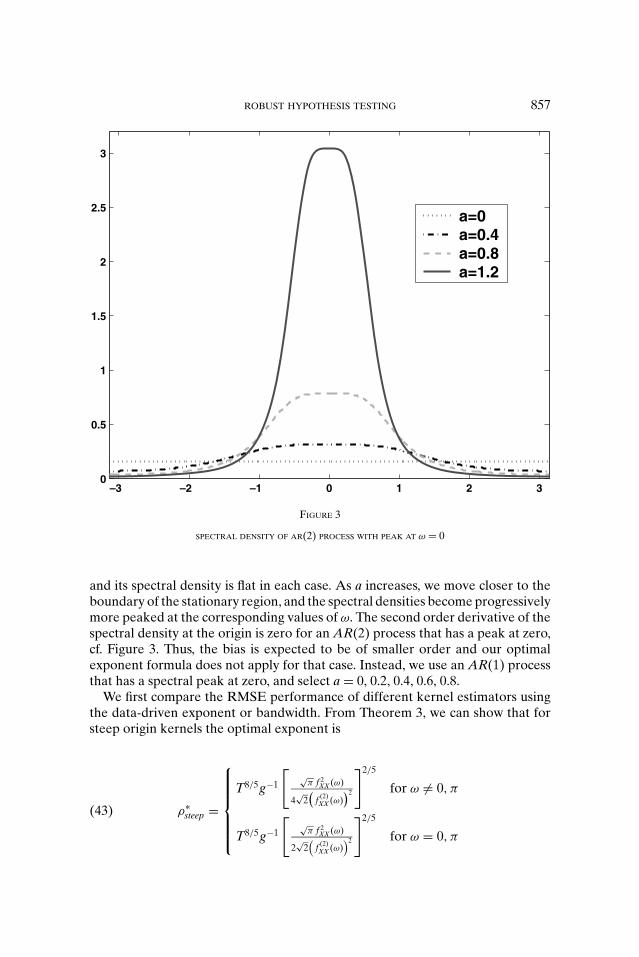
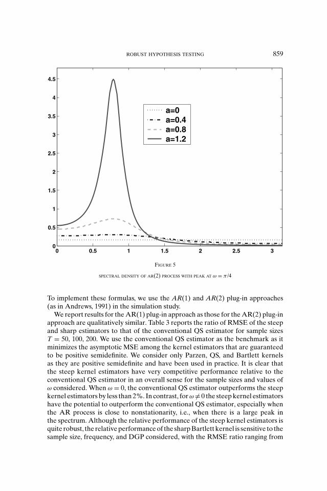
2) for a peak at ω = π /4. Accordingly, for our simulations, we selecta = 0, 0.4, 0.8, 1.2, 1.6 in the second case, and a = 0, 0.4, 0.8, 1.2 in the third case,together with b = a/(a − 4 cos ω) for different values of ω. Figures 3–5 display thecorresponding spectral densities of the Xt process with peaks at ω = 0, π /6, andπ /4, respectively, for a = 0, 0.4, 0.8, and 1.2. When a = 0, the process is white noise
ROBUST HYPOTHESIS TESTING 857
–3 –2 –1 0 1 2 30
0.5
1
1.5
2
2.5
3
a=0a=0.4a=0.8a=1.2
FIGURE 3
SPECTRAL DENSITY OF AR(2) PROCESS WITH PEAK AT ω = 0
and its spectral density is flat in each case. As a increases, we move closer to theboundary of the stationary region, and the spectral densities become progressivelymore peaked at the corresponding values of ω. The second order derivative of thespectral density at the origin is zero for an AR(2) process that has a peak at zero,cf. Figure 3. Thus, the bias is expected to be of smaller order and our optimalexponent formula does not apply for that case. Instead, we use an AR(1) processthat has a spectral peak at zero, and select a = 0, 0.2, 0.4, 0.6, 0.8.
We first compare the RMSE performance of different kernel estimators usingthe data-driven exponent or bandwidth. From Theorem 3, we can show that forsteep origin kernels the optimal exponent is
ρ∗steep =
⎧⎪⎪⎪⎪⎪⎨⎪⎪⎪⎪⎪⎩T8/5g−1
[√
π f 2XX (ω)
4√
2(
f (2)XX (ω)
)2
]2/5
for ω �= 0, π
T8/5g−1
[√
π f 2XX (ω)
2√
2(
f (2)XX (ω)
)2
]2/5
for ω = 0, π
(43)

858 PHILLIPS, SUN, AND JIN
0 0.5 1 1.5 2 2.5 30
0.5
1
1.5
2
a=0a=0.4a=0.8a=1.2
FIGURE 4
SPECTRAL DENSITY OF AR(2) PROCESS WITH PEAK AT ω = π /6
An analogous analysis shows that for sharp origin kernels the optimal exponentis
ρ∗sharp =
⎧⎪⎪⎪⎪⎪⎨⎪⎪⎪⎪⎪⎩T2/3
[f 2XX (ω)
2(
f (1)XX (ω)
)2
]1/3
for ω �= 0, π
T2/3
[f 2XX (ω)(
f (1)XX (ω)
)2
]1/3
for ω = 0, π
(44)
and, for the conventional estimator with the QS kernel the optimal bandwidth is
ST =
⎧⎪⎪⎪⎪⎪⎨⎪⎪⎪⎪⎪⎩1.3221T1/5
[2(
f (2)XX (ω)
)2
f 2XX (ω)
]1/5
for ω �= 0, π
1.3221T1/5
[(f (2)XX (ω)
)2
f 2XX (ω)
]1/5
for ω = 0, π
(45)
ROBUST HYPOTHESIS TESTING 859
0 0.5 1 1.5 2 2.5 30
0.5
1
1.5
2
2.5
3
3.5
4
4.5
a=0a=0.4a=0.8a=1.2
FIGURE 5
SPECTRAL DENSITY OF AR(2) PROCESS WITH PEAK AT ω = π /4
To implement these formulas, we use the AR(1) and AR(2) plug-in approaches(as in Andrews, 1991) in the simulation study.
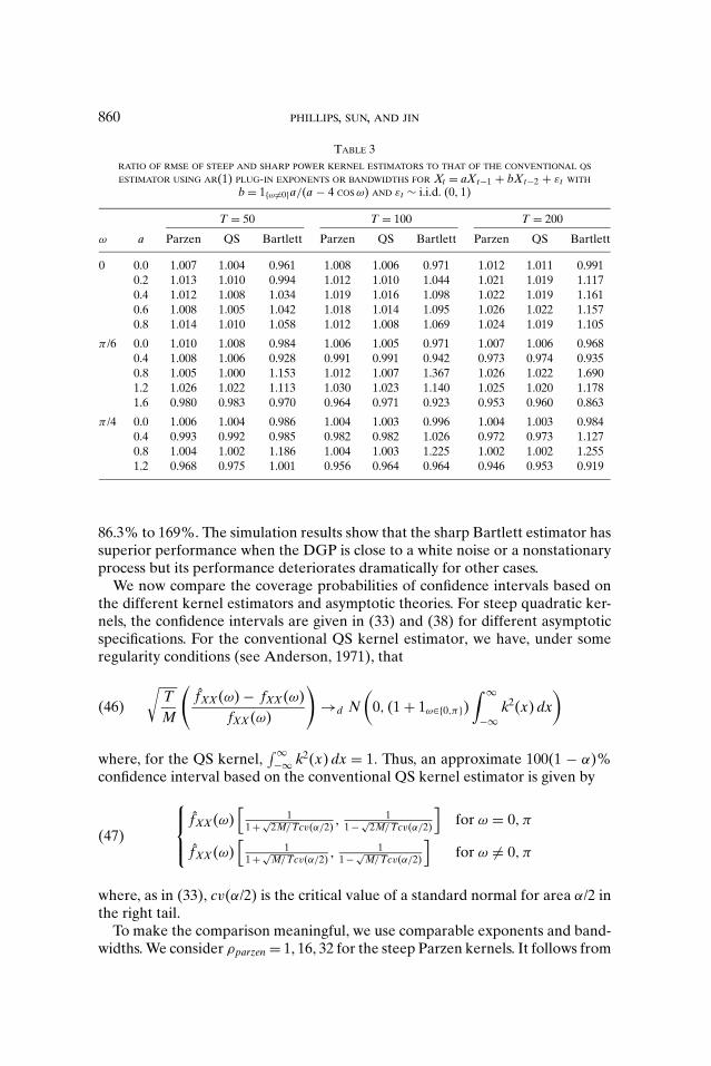
We report results for the AR(1) plug-in approach as those for the AR(2) plug-inapproach are qualitatively similar. Table 3 reports the ratio of RMSE of the steepand sharp estimators to that of the conventional QS estimator for sample sizesT = 50, 100, 200. We use the conventional QS estimator as the benchmark as itminimizes the asymptotic MSE among the kernel estimators that are guaranteedto be positive semidefinite. We consider only Parzen, QS, and Bartlett kernelsas they are positive semidefinite and have been used in practice. It is clear thatthe steep kernel estimators have very competitive performance relative to theconventional QS estimator in an overall sense for the sample sizes and values ofω considered. When ω = 0, the conventional QS estimator outperforms the steepkernel estimators by less than 2%. In contrast, for ω �= 0 the steep kernel estimatorshave the potential to outperform the conventional QS estimator, especially whenthe AR process is close to nonstationarity, i.e., when there is a large peak inthe spectrum. Although the relative performance of the steep kernel estimators isquite robust, the relative performance of the sharp Bartlett kernel is sensitive to thesample size, frequency, and DGP considered, with the RMSE ratio ranging from
860 PHILLIPS, SUN, AND JIN
TABLE 3
RATIO OF RMSE OF STEEP AND SHARP POWER KERNEL ESTIMATORS TO THAT OF THE CONVENTIONAL QS
ESTIMATOR USING AR(1) PLUG-IN EXPONENTS OR BANDWIDTHS FOR Xt = aXt−1 + bXt−2 + εt WITH
b = 1{ω �=0}a/(a − 4 COS ω) AND εt ∼ i.i.d. (0, 1)
T = 50 T = 100 T = 200
ω a Parzen QS Bartlett Parzen QS Bartlett Parzen QS Bartlett
0 0.0 1.007 1.004 0.961 1.008 1.006 0.971 1.012 1.011 0.991
0.2 1.013 1.010 0.994 1.012 1.010 1.044 1.021 1.019 1.117
0.4 1.012 1.008 1.034 1.019 1.016 1.098 1.022 1.019 1.161
0.6 1.008 1.005 1.042 1.018 1.014 1.095 1.026 1.022 1.157
0.8 1.014 1.010 1.058 1.012 1.008 1.069 1.024 1.019 1.105
π /6 0.0 1.010 1.008 0.984 1.006 1.005 0.971 1.007 1.006 0.968
0.4 1.008 1.006 0.928 0.991 0.991 0.942 0.973 0.974 0.935
0.8 1.005 1.000 1.153 1.012 1.007 1.367 1.026 1.022 1.690
1.2 1.026 1.022 1.113 1.030 1.023 1.140 1.025 1.020 1.178
1.6 0.980 0.983 0.970 0.964 0.971 0.923 0.953 0.960 0.863
π /4 0.0 1.006 1.004 0.986 1.004 1.003 0.996 1.004 1.003 0.984
0.4 0.993 0.992 0.985 0.982 0.982 1.026 0.972 0.973 1.127
0.8 1.004 1.002 1.186 1.004 1.003 1.225 1.002 1.002 1.255
1.2 0.968 0.975 1.001 0.956 0.964 0.964 0.946 0.953 0.919
86.3% to 169%. The simulation results show that the sharp Bartlett estimator hassuperior performance when the DGP is close to a white noise or a nonstationaryprocess but its performance deteriorates dramatically for other cases.
We now compare the coverage probabilities of confidence intervals based onthe different kernel estimators and asymptotic theories. For steep quadratic ker-nels, the confidence intervals are given in (33) and (38) for different asymptoticspecifications. For the conventional QS kernel estimator, we have, under someregularity conditions (see Anderson, 1971), that√
TM
(fXX(ω) − fXX(ω)
fXX(ω)
)→d N
(0, (1 + 1ω∈{0,π})
∫ ∞
−∞k2(x) dx
)(46)
where, for the QS kernel,∫ ∞−∞ k2(x) dx = 1. Thus, an approximate 100(1 − α)%
confidence interval based on the conventional QS kernel estimator is given by⎧⎪⎨⎪⎩fXX(ω)
[1
1 + √2M/Tcv(α/2)
, 11 − √
2M/Tcv(α/2)
]for ω = 0, π
fXX(ω)[
11 + √
M/Tcv(α/2), 1
1 − √M/Tcv(α/2)
]for ω �= 0, π
(47)
where, as in (33), cv(α/2) is the critical value of a standard normal for area α/2 inthe right tail.
To make the comparison meaningful, we use comparable exponents and band-widths. We consider ρparzen = 1, 16, 32 for the steep Parzen kernels. It follows from

ROBUST HYPOTHESIS TESTING 861
TABLE 4
FINITE SAMPLE COVERAGES AND RELATIVE LENGTHS OF DIFFERENT 95% CONFIDENCE INTERVALS FOR
SPECTRAL DENSITIES AT DIFFERENT FREQUENCIES WHEN Xt = aXt−1 + bXt−2 + εt WITH b = 1{ω �=0}a/
(a − 4 COS ω) AND εt ∼ i.i.d. (0, 1)a,b
Fixed-ρParzen Large-ρ Parzen Fixed-ρ QS Large-ρ QSQS
Coverage Length Coverage Length Coverage Length Coverage Length Coverage
ω a T = 100
0 0.0 0.950 0.000 0.998 0.894 0.950 0.000 0.998 0.935 0.995
0.2 0.948 0.000 0.998 0.892 0.950 0.000 0.998 0.939 0.996
0.4 0.949 0.000 0.998 0.890 0.951 0.000 0.998 0.934 0.996
0.6 0.951 0.000 0.998 0.889 0.952 0.000 0.996 0.934 0.996
0.8 0.947 0.000 0.999 0.880 0.950 0.000 0.998 0.925 0.998
π /4 0.0 0.863 0.000 0.959 0.986 0.868 0.000 0.962 0.990 0.961
0.4 0.861 0.000 0.959 0.987 0.864 0.000 0.962 0.990 0.961
0.8 0.857 0.000 0.961 0.981 0.861 0.000 0.964 0.988 0.963
1.2 0.829 0.000 0.969 0.99 0.832 0.000 0.972 0.993 0.971
ω a T = 200
0 0.0 0.953 0.000 0.998 0.894 0.954 0.000 0.998 0.937 0.996
0.2 0.953 0.000 0.998 0.891 0.954 0.000 0.998 0.932 0.997
0.4 0.953 0.000 0.998 0.892 0.954 0.000 0.998 0.933 0.997
0.6 0.953 0.000 0.998 0.893 0.955 0.000 0.998 0.938 0.997
0.8 0.953 0.000 0.998 0.889 0.955 0.000 0.998 0.933 0.997
π /4 0.0 0.864 0.000 0.959 0.986 0.868 0.000 0.962 0.990 0.961
0.4 0.861 0.000 0.959 0.987 0.864 0.000 0.962 0.990 0.961
0.8 0.857 0.000 0.961 0.981 0.861 0.000 0.964 0.988 0.963
1.2 0.829 0.000 0.969 0.990 0.832 0.000 0.972 0.993 0.971
aThe exponents for the steep Parzen and QS kernels are 1 and 4, respectively.bThe bandwidth for the conventional QS kernel is T/2.
Equation (14) that the comparable exponents for the steep QS kernel are ρQS =4, 67, and 135. For these values of ρQS, we choose the bandwidth according toM = T/
√ρQS. Such a bandwidth choice rule ensures that the local behavior of
kQS,ρ(x/T) at the origin matches that of kQS(x/M).For each data generating process and exponent or bandwidth, we compute
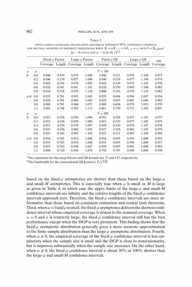
fXX(ω) and construct the confidence intervals using (33), (38), or (47) for T =50, 100, 200. To evaluate the information content of these confidence intervals,we calculate their lengths. Obviously, the shorter a confidence interval is, the moreinformative it is. We focus on the steep Parzen and QS kernel estimators underthe fixed and large ρ asymptotics and the conventional QS kernel estimator underthe usual “small-M” asymptotics given in (46). Tables 4 and 5 report the finite sam-ple coverages and relative lengths of different 95% confidence intervals for T =100 and 200 based on 10,000 replications. The length reported is the median lengthover the 10,000 replications divided by the median length of the conventional QSconfidence interval.
We draw attention to four aspects of Tables 4 and 5. First, for the confidenceinterval constructed using the asymptotic normality results, the length and finitesample coverages are more or less the same. Second, the confidence intervals
862 PHILLIPS, SUN, AND JIN
TABLE 5
FINITE SAMPLE COVERAGES AND RELATIVE LENGTHS OF DIFFERENT 95% CONFIDENCE INTERVALS
FOR SPECTRAL DENSITIES AT DIFFERENT FREQUENCIES WHEN Xt = aXt−1 + bXt−2 + εt WITH b = 1{ω �=0}a/
(a − 4 COS ω) AND εt ∼ i.i.d. (0, 1)a,b
Fixed-ρ Parzen Large-ρ Parzen Fixed-ρ QS Large-ρ QSQS
Coverage Length Coverage Length Coverage Length Coverage Length Coverage
ω a T = 100
0 0.0 0.948 0.539 0.975 1.098 0.946 0.531 0.976 1.108 0.973
0.2 0.946 0.538 0.977 1.096 0.946 0.528 0.977 1.104 0.974
0.4 0.943 0.538 0.978 1.095 0.942 0.528 0.979 1.102 0.978
0.6 0.928 0.541 0.981 1.101 0.928 0.530 0.983 1.108 0.983
0.8 0.816 0.558 0.970 1.136 0.808 0.543 0.970 1.134 0.963
π /4 0.0 0.935 0.701 0.955 1.045 0.935 0.694 0.956 1.047 0.954
0.4 0.928 0.701 0.960 1.045 0.929 0.693 0.962 1.046 0.962
0.8 0.888 0.701 0.968 1.055 0.888 0.698 0.970 1.053 0.970
1.2 0.481 0.748 0.765 1.115 0.461 0.730 0.757 1.103 0.697
ω a T = 200
0 0.0 0.952 0.538 0.976 1.096 0.952 0.529 0.977 1.105 0.975
0.2 0.952 0.538 0.976 1.096 0.951 0.529 0.977 1.105 0.975
0.4 0.951 0.539 0.978 1.097 0.949 0.530 0.978 1.107 0.976
0.6 0.947 0.538 0.981 1.095 0.947 0.528 0.981 1.103 0.979
0.8 0.923 0.542 0.985 1.103 0.922 0.531 0.987 1.109 0.984
π /4 0.0 0.934 0.702 0.952 1.046 0.934 0.695 0.955 1.049 0.955
0.4 0.931 0.703 0.954 1.048 0.931 0.695 0.956 1.049 0.957
0.8 0.925 0.703 0.958 1.047 0.924 0.695 0.961 1.049 0.963
1.2 0.800 0.720 0.944 1.074 0.792 0.707 0.945 1.068 0.938
aThe exponents for the steep Parzen and QS kernels are 32 and 135, respectively.bThe bandwidth for the conventional QS kernel is T/
√135.
based on the fixed-ρ asymptotics are shorter than those based on the large-ρand small-M asymptotics. This is especially true when ρ is small or M is largeas given in Table 4, in which case the upper limits of the large-ρ and small-Mconfidence intervals are infinity and the relative lengths of the fixed-ρ confidenceintervals approach zero. Therefore, the fixed-ρ confidence intervals are more in-formative than those based on consistent estimation and central limit theorems.Third, when ω = 0 and ρ is small, the fixed-ρ asymptotics delivers the shortest confi-dence interval whose empirical coverage is closest to the nominal coverage. Whenω = 0 and ρ is relatively large, the fixed-ρ confidence interval still has the bestperformance except when the DGP is very persistent. This finding shows that thefixed-ρ asymptotic distribution generally gives a more accurate approximationto the finite sample distribution than the large-ρ asymptotic distribution. Fourth,when ω �= 0, the empirical coverage of the fixed-ρ confidence interval is less sat-isfactory when the sample size is small and the DGP is close to nonstationarity,but it improves substantially when the sample size increases. On the other hand,when ω �= 0, the fixed-ρ confidence interval is about 30% or 100% shorter thanthe large-ρ and small-M confidence intervals.

ROBUST HYPOTHESIS TESTING 863
To sum up, the fixed-ρ steep-kernel-based confidence interval is the best in anoverall sense when ρ is not large.
5.2. Robust Hypothesis Testing. Using the steep kernel LRV estimator, wepropose a new approach to robust hypothesis testing. Consider the linear regres-sion model
yt = z′tβ + ut , t = 1, 2, . . . , T(48)
where ut is autocorrelated and possibly conditionally heteroskedastic and zt is anm × 1 vector of regressors. Suppose we want to test the null H0 : Rβ = r againstthe alternative H1 : Rβ �= r where R is a p × m matrix. Let β be the OLS estimatorand Q be 1/T
∑Tt=1 zt z′
t . Then the usual F-statistic is
F∗ρ = T(Rβ − r)′(RQ−1�ρ Q−1 R′)−1
(Rβ − r)/
p(49)
or, when p = 1, the t-ratio is
t∗ρ = T1/2(Rβ − r)
(RQ−1�ρ Q−1 R′)−1/2
(50)
where �ρ = 2π fXX(0), f XX(0) is defined in (2) with Xt replaced by zt (yt − z′t β).
Let ρ be the data-driven exponent as defined in (20) with α replaced by thefirst order autocorrelation of Xt. Using the results in the previous sections andfollowing the arguments similar to the proof of Theorem 3 in PSJ (2003), we canshow that under Assumptions 1–3,
pF∗ρ ⇒ W′
p(1)Wp(1) =d χ2p, t∗
ρ ⇒ W1(1) =d N(0, 1)(51)
under the null hypothesis, and
pF∗ρ ⇒ (
�∗−1c + Wp(1))′(
�∗−1c + Wp(1)), t∗
ρ ⇒ (γ + W1(1))(52)
under the local alternative hypothesis H1 : Rβ = r + cT−1/2. Here �∗�∗′ =RQ−1�Q−1 R′, γ = c(RQ−1 �Q−1 R′)−1/2, and Wp(r) is p-dimensional standardBrownian motion.
The above limiting distributions hold under the large-ρ asymptotics in whichthe exponent ρ approaches infinity at a suitable rate so that we have consistentHAC estimates. It is known that consistent HAC estimates are not needed inorder to produce asymptotically valid tests. Using Theorem 6, we can show thatthe F∗
ρ and t∗ρ statistics have the following limiting distributions under the fixed-ρ
asymptotics. First, under the null H0 : Rβ = r ,

864 PHILLIPS, SUN, AND JIN
pF∗ρ ⇒ W′
p(1)
(∫ 1
0
∫ 1
0
k∗ρ(r − s) dWp(r) dW ′
p(s)
)−1
Wp(1)
:= W′p(1)
(∫ 1
0
∫ 1
0
kρ(r − s) dVp(r) dV′p(s)
)−1
Wp(1)
(53)
and
t∗ρ ⇒ W1(1)
(∫ 1
0
∫ 1
0
kρ(r − s) dV1(r) dV′1(s)
)−1/2
(54)
Second, under the local alternative H1 : Rβ = r + cT−1/2,
pF∗ρ ⇒ (
�∗−1c + Wp(1))′
(∫ 1
0
∫ 1
0
kρ(r − s) dVp(r) dV′p(s)
)−1 (�∗−1c + Wp(1)
)(55)
and
t∗ρ ⇒ (γ + W1(1))
(∫ 1
0
∫ 1
0
kρ(r − s) dV1(r) dV1(s)
)−1/2
(56)
In these formulas, kρ(·) is any positive semidefinite kernel (so the steep Parzenand QS kernels may be used), and Vp(r) is p-dimensional standard Brownianbridge. For derivations of the preceding formulas, see PSJ (2003).
Given the above fixed-ρ asymptotics, the critical values for different ρ valuescan be simulated and tabulated. As in Table 2, we approximate the Brownianmotion by normalized partial sums of 1,000 i.i.d. N(0, 1) random variables andsimulate the t∗
ρ statistic 10,000 times. It turns out that the critical values at a givensignificance level can be represented approximately by a hyperbola (as a functionof
√ρ) of the following form:
cv = b√ρ − a
+ c(57)
where c is the critical value from the standard normal. Table 6 presents nonlinearleast squares estimates of a and b, the standard errors, and R2 (see (40) for the for-mulas) of the nonlinear regressions. For both Parzen and QS kernels, the standarderrors are small and the R2s are close to 1, indicating that the hyperbola representsthe critical values very well. The hyperbola becomes nearly flat for large ρ, andthe fitted critical values are very close to those from the standard normal as ρ →∞. This is not surprising as the t-statistic is asymptotically normal under large-ρasymptotics.

ROBUST HYPOTHESIS TESTING 865
TABLE 6
ASYMPTOTIC CRITICAL VALUE FUNCTIONS FOR THE ONE-SIDED t∗ρ -TEST WITH STEEP PARZEN AND QS KERNELS
Parzen QS
90.0% 95.0% 97.5% 99.0% 90.0% 95.0% 97.5% 99.0%
a 0.480 0.503 0.480 0.460 0.478 0.500 0.542 0.591
b 0.807 1.289 1.967 3.002 2.113 3.336 4.824 6.986
c 1.282 1.645 1.960 2.326 1.282 1.645 1.960 2.326
s.e. 0.0229 0.0339 0.0290 0.0647 0.0217 0.0410 0.0604 0.0744
R2 0.9997 0.9996 0.9998 0.9994 0.9998 0.9996 0.9994 0.9994
We now proceed to investigate the asymptotic power of the t∗ test under bothfixed-ρ asymptotics and large-ρ asymptotics. For convenience, we refer to thesetwo tests as the t∗
ρ test and the t∗ρ test, respectively. Note that for a given exponent
the t-statistic is constructed in exactly the same way regardless of the asymptoticsused. The difference between the two tests is that for the t∗
ρ test the exponent isfixed a priori and critical values from the fixed-ρ asymptotics are used, whereasfor the t∗
ρ test the exponent is data driven and critical values from the large-ρasymptotics are used. For the t∗
ρ test, the power curve is the same as the powerenvelope that is obtained when the true � or any consistent estimate is used.This holds because the consistency approximation is being used. For the t∗
ρ test,we consider three values of ρ: ρ = 1, 16, and 32 for the steep Parzen kerneland ρ = 6, 96, and 192 for the steep QS kernel. For each ρ, we approximate theBrownian motion and Brownian bridge processes by the partial sums of 1,000normal variates.
Figure 6 presents the asymptotic power curves when the steep Parzen kernel isused. The figure is based on 50,000 simulation replications. It is apparent that thepower curve moves up uniformly as ρ increases, just as it does with sharp originkernels (PSJ, 2003). The difference is that with sharp origin kernels, when ρ ≥16, the power curve is very close to the power envelope, whereas much largervalues of ρ are needed here, consonant with the power parameter expansion ratesestablished for consistent HAC estimation earlier in the article. To save space,we do not report the local power curves when the steep QS kernel is used butinstead comment on it briefly. The curves are similar to those in Figure 6 but weneed to take a larger ρ to attain the same power. This result is consistent with thecurvature difference at the origin between the Parzen and QS kernels.
Compared with the t∗ρ test, the t∗
ρ test has an obvious power advantage. However,as with other tests that use consistent LRV estimates, the t∗
ρ test has larger sizedistortion than the t∗
ρ test in finite samples. Before studying the finite sampleperformances of these two tests, we introduce a new test that seeks to combinethe good elements of both procedures. The new test uses the same t∗
ρ statisticdefined in (50) with a data-driven ρ. The point of departure is that, instead ofusing the critical values from the standard normal, we propose using the criticalvalues from the hyperbola defined in (57). The new testing procedure is thus a

866 PHILLIPS, SUN, AND JIN
0 0.5 1 1.5 2 2.5 3 3.5 4 4.5 50
0.1
0.2
0.3
0.4
0.5
0.6
0.7
0.8
0.9
1
γ
Po
wer
t*ρ^ test
t*ρ=1 test
t*ρ=16 test
t*ρ=32 test
FIGURE 6
ASYMPTOTIC LOCAL POWER FUNCTION OF THE t∗ TESTS WITH THE STEEP PARZEN KERNEL
mixture of the t∗ρ test and the t∗
ρ test. As a result, the new test has the dual advantageof an optimal choice of power parameter that is data determined and at the sametime the good finite sample size properties of the t∗
ρ test. The latter point willbecome clear below. Since the critical value from the hyperbola approaches thatof the standard normal as ρ → ∞, the new test is equivalent to the t∗
ρ test in largesamples. We will refer to the new test as the t∗
new test hereafter.Kiefer and Vogelsang (2005) employ a similar strategy to combine the good
elements of the standard asymptotic normality test and the nonstandard test inwhich the bandwidth is set proportional to the sample size. More specifically,they first compute the data-driven AMSE optimal bandwidth M using the AR(1)plug-in procedure (Andrews, 1991) and then use the ratio b = M/T to obtain thenonstandard critical value from their fixed-b asymptotics. Kiefer and Vogelsangshow that the nonstandard critical value can be approximated very well by apolynomial in b. For convenience, the Kiefer and Vogelsang test that uses thepolynomial approximation will be called the t∗
KV test.It is important to point out that the AMSE optimal power parameter ρ or
bandwidth parameter M is not necessarily optimal in balancing the type I andtype II errors of the t-test. We are content with the AMSE criterion here and leave
ROBUST HYPOTHESIS TESTING 867
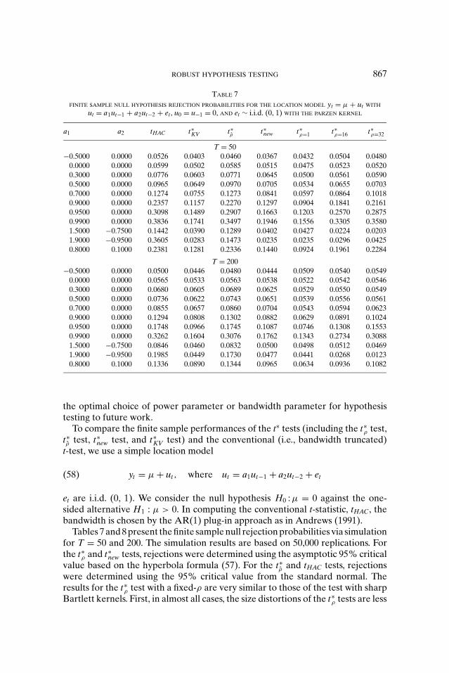
TABLE 7
FINITE SAMPLE NULL HYPOTHESIS REJECTION PROBABILITIES FOR THE LOCATION MODEL yt = μ + ut WITH
ut = a1ut−1 + a2ut−2 + et , u0 = u−1 = 0, AND et ∼ i.i.d. (0, 1) WITH THE PARZEN KERNEL
a1 a2 tHAC t∗KV t∗ρ t∗new t∗ρ=1 t∗
ρ=16 t∗ρ=32
T = 50
−0.5000 0.0000 0.0526 0.0403 0.0460 0.0367 0.0432 0.0504 0.0480
0.0000 0.0000 0.0599 0.0502 0.0585 0.0515 0.0475 0.0523 0.0520
0.3000 0.0000 0.0776 0.0603 0.0771 0.0645 0.0500 0.0561 0.0590
0.5000 0.0000 0.0965 0.0649 0.0970 0.0705 0.0534 0.0655 0.0703
0.7000 0.0000 0.1274 0.0755 0.1273 0.0841 0.0597 0.0864 0.1018
0.9000 0.0000 0.2357 0.1157 0.2270 0.1297 0.0904 0.1841 0.2161
0.9500 0.0000 0.3098 0.1489 0.2907 0.1663 0.1203 0.2570 0.2875
0.9900 0.0000 0.3836 0.1741 0.3497 0.1946 0.1556 0.3305 0.3580
1.5000 −0.7500 0.1442 0.0390 0.1289 0.0402 0.0427 0.0224 0.0203
1.9000 −0.9500 0.3605 0.0283 0.1473 0.0235 0.0235 0.0296 0.0425
0.8000 0.1000 0.2381 0.1281 0.2336 0.1440 0.0924 0.1961 0.2284
T = 200
−0.5000 0.0000 0.0500 0.0446 0.0480 0.0444 0.0509 0.0540 0.0549
0.0000 0.0000 0.0565 0.0533 0.0563 0.0538 0.0522 0.0542 0.0546
0.3000 0.0000 0.0680 0.0605 0.0689 0.0625 0.0529 0.0550 0.0549
0.5000 0.0000 0.0736 0.0622 0.0743 0.0651 0.0539 0.0556 0.0561
0.7000 0.0000 0.0855 0.0657 0.0860 0.0704 0.0543 0.0594 0.0623
0.9000 0.0000 0.1294 0.0808 0.1302 0.0882 0.0629 0.0891 0.1024
0.9500 0.0000 0.1748 0.0966 0.1745 0.1087 0.0746 0.1308 0.1553
0.9900 0.0000 0.3262 0.1604 0.3076 0.1762 0.1343 0.2734 0.3088
1.5000 −0.7500 0.0846 0.0460 0.0832 0.0500 0.0498 0.0512 0.0469
1.9000 −0.9500 0.1985 0.0449 0.1730 0.0477 0.0441 0.0268 0.0123
0.8000 0.1000 0.1336 0.0890 0.1344 0.0965 0.0634 0.0936 0.1082
the optimal choice of power parameter or bandwidth parameter for hypothesistesting to future work.
To compare the finite sample performances of the t∗ tests (including the t∗ρ test,
t∗ρ test, t∗
new test, and t∗KV test) and the conventional (i.e., bandwidth truncated)
t-test, we use a simple location model
yt = μ + ut , where ut = a1ut−1 + a2ut−2 + et(58)
et are i.i.d. (0, 1). We consider the null hypothesis H0 : μ = 0 against the one-sided alternative H1 : μ > 0. In computing the conventional t-statistic, tHAC, thebandwidth is chosen by the AR(1) plug-in approach as in Andrews (1991).
Tables 7 and 8 present the finite sample null rejection probabilities via simulationfor T = 50 and 200. The simulation results are based on 50,000 replications. Forthe t∗
ρ and t∗new tests, rejections were determined using the asymptotic 95% critical
value based on the hyperbola formula (57). For the t∗ρ and tHAC tests, rejections
were determined using the 95% critical value from the standard normal. Theresults for the t∗
ρ test with a fixed-ρ are very similar to those of the test with sharpBartlett kernels. First, in almost all cases, the size distortions of the t∗
ρ tests are less
868 PHILLIPS, SUN, AND JIN
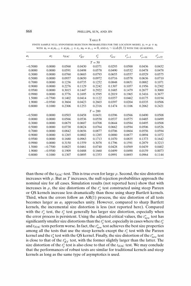
TABLE 8
FINITE SAMPLE NULL HYPOTHESIS REJECTION PROBABILITIES FOR THE LOCATION MODEL yt = μ + utWITH ut = a1ut−1 + a2ut−2 + et , u0 = u−1 = 0, AND et ∼ i.i.d.(0, 1) WITH THE QS KERNEL
a1 a2 tHAC t∗KV t∗ρ t∗new t∗ρ=1 t∗
ρ=16 t∗ρ=32
T = 50
−0.5000 0.0000 0.0568 0.0430 0.0371 0.0293 0.0500 0.0436 0.0432
0.0000 0.0000 0.0591 0.0498 0.0578 0.0490 0.0532 0.0478 0.0478
0.3000 0.0000 0.0760 0.0603 0.0793 0.0655 0.0557 0.0529 0.0575
0.5000 0.0000 0.0937 0.0650 0.0972 0.0716 0.0578 0.0636 0.0710
0.7000 0.0000 0.1236 0.0735 0.1252 0.0848 0.0651 0.0882 0.1071
0.9000 0.0000 0.2276 0.1129 0.2242 0.1307 0.1057 0.1956 0.2302
0.9500 0.0000 0.3015 0.1447 0.2922 0.1685 0.1479 0.2677 0.3000
0.9900 0.0000 0.3776 0.1695 0.3595 0.2019 0.1965 0.3416 0.3677
1.5000 −0.7500 0.1402 0.0414 0.1122 0.0357 0.0462 0.0175 0.0194
1.9000 −0.9500 0.3604 0.0423 0.2603 0.0397 0.0204 0.0335 0.0506
0.8000 0.1000 0.2306 0.1253 0.2316 0.1474 0.1106 0.2062 0.2421
T = 200
−0.5000 0.0000 0.0503 0.0458 0.0431 0.0396 0.0566 0.0490 0.0508
0.0000 0.0000 0.0566 0.0536 0.0558 0.0537 0.0575 0.0485 0.0499
0.3000 0.0000 0.0679 0.0607 0.0708 0.0644 0.0584 0.0495 0.0508
0.5000 0.0000 0.0738 0.0624 0.0764 0.0662 0.0594 0.0506 0.0526
0.7000 0.0000 0.0842 0.0656 0.0877 0.0706 0.0604 0.0556 0.0594
0.9000 0.0000 0.1265 0.0802 0.1285 0.0880 0.0677 0.0894 0.1072
0.9500 0.0000 0.1680 0.0963 0.1713 0.1070 0.0835 0.1373 0.1642
0.9900 0.0000 0.3150 0.1559 0.3078 0.1796 0.1591 0.2879 0.3213
1.5000 −0.7500 0.0825 0.0461 0.0740 0.0428 0.0569 0.0439 0.0402
1.9000 −0.9500 0.1909 0.0488 0.1660 0.0499 0.0490 0.0159 0.0073
0.8000 0.1000 0.1307 0.0895 0.1353 0.0991 0.0693 0.0964 0.1144
than those of the tHAC-test. This is true even for large ρ. Second, the size distortionincreases with ρ. But as T increases, the null rejection probabilities approach thenominal size for all cases. Simulation results (not reported here) show that withincreases in ρ, the size distortions of the t∗
ρ test constructed using steep Parzenor QS kernels increase less dramatically than those using sharp Bartlett kernels.Third, when the errors follow an AR(1) process, the size distortion of all testsbecomes larger as a1 approaches unity. However, compared to sharp Bartlettkernels, the incremental size distortion is less (not reported here). Comparedwith the t∗
ρ test, the t∗ρ test generally has larger size distortion, especially when
the error process is persistent. Using the adjusted critical values, the t∗new test has
significantly smaller size distortions than the t∗ρ test, especially in cases where the t∗
ρ
and tHAC tests perform worse. In fact, the t∗new test achieves the best size properties
among all the tests that use the steep kernels except the t∗1 test with the Parzen
kernel and the t∗6 test with the QS kernel. Finally, the size distortion of the t∗
new testis close to that of the t∗
KV test, with the former slightly larger than the latter. Thesize distortion of the t∗
ρ test is also close to that of the tHAC test. We may concludethat the performances of robust tests are similar for traditional kernels and steepkernels as long as the same type of asymptotics is used.
ROBUST HYPOTHESIS TESTING 869
0 0.5 1 1.5 2 2.5 30
0.1
0.2
0.3
0.4
0.5
0.6
0.7
0.8
0.9
1
μ
Po
we
r
tHAC
test
t*KV
test
t*ρ^
test
t*new
test
t*ρ=1
test
t*ρ=16
test
t*ρ=32
test
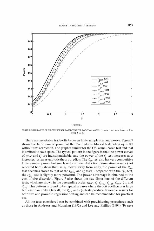
FIGURE 7
FINITE SAMPLE POWER OF PARZEN-KERNEL-BASED TEST FOR LOCATION MODEL: yt = μ + ut , ut = 0.7ut−1 + etWITH T = 50
There are inevitable trade-offs between finite sample size and power. Figure 7shows the finite sample power of the Parzen-kernel-based tests when a1 = 0.7without size correction. The graph is similar for the QS-kernel-based test and thatis omitted to save space. The typical pattern in the figure is that the power curvesof tHAC and t∗
ρ are indistinguishable, and the power of the t∗ρ test increases as ρ
increases, just as asymptotic theory predicts. The t∗new test also has very competitive
finite sample power but much reduced size distortion. Simulation results (notreported here) show that, as a1 moves away from unity, the power of the t∗
newtest becomes closer to that of the tHAC and t∗
ρ tests. Compared with the t∗KV test,
the t∗new test is slightly more powerful. The power advantage is obtained at the
cost of size distortion. Figure 7 also shows the size distortions of the differenttests, which are shown in the descending order: tHAC, t∗
ρ , t∗ρ=32, t∗
ρ=16, t∗new, t∗
KV , andt∗ρ=1. This pattern is found to be typical in cases where the AR coefficient is large
but less than unity. Overall, the t∗new and t∗
KV tests produce favorable results forboth size and power in regression testing and can be recommended for practicaluse.
All the tests considered can be combined with prewhitening procedures suchas those in Andrews and Monahan (1992) and Lee and Phillips (1994). To save

870 PHILLIPS, SUN, AND JIN
space, we do not report the simulation results for the prewhitening version forthe tests. We remark that, when AR(1) prewhitening is used, all the qualitativeobservations continue to apply but the size distortions are smaller in all cases. Thisis because the AR(1) filter is effective in reducing the high autocorrelation in theautoregressive DGPs.
6. EXTENSIONS AND CONCLUSION
Exponentiating a mother kernel enables consistent kernel estimation withoutthe use of lag truncation. When the exponent parameter is not too large, theabsence of lag truncation influences the variability of the estimate because ofthe presence of autocovariances at long lags. As has been noted by Kiefer andVogelsang (2002a, 2002b) and Jansson (2004) and as confirmed in the simulationsreported here, such effects can have the advantage of better reflecting finite sam-ple behavior in test statistics that employ LRV/HAC estimates leading to someimprovement in test size. When the exponent is passed to infinity with the sam-ple size, the kernels produce consistent LRV/HAC and spectral density estimates,thereby ensuring that there is no loss in test power asymptotically. Similar ideascan, of course, be used in probability density estimation and in nonparametricregression.
One feature of interest in the asymptotic theory is that, unlike conventionalkernel estimation where an optimal choice of quadratic kernel is possible in termsof MSE criteria, steep origin kernels are asymptotically MSE equivalent, so thatchoice of mother kernel does not matter asymptotically, although it may of coursedo so in finite samples. Another feature of the asymptotic theory of steep originkernel estimation is that optimal convergence rates (that minimize an asymp-totic MSE criterion) are faster for quadratic mother kernels than they are forthe Bartlett kernel. The corresponding expansion rate for the exponent is ρ =O(T8/5) (leading to a convergence rate of T2/5 for the kernel estimate fXX) sothat ρ tends to infinity much faster than the sample size T. The reason for this fastexpansion rate is that quadratic kernels have a flat shape at the origin and, sinceno bandwidth or lag truncation is being employed to control the effect of sam-ple autocovariances at long lags, the fast rate of exponentiation ensures that thelong lag sample autocovariances are sufficiently downweighted for a central limittheory to apply. The use of flat top kernels with bandwidth parameters and steepdecay at long lags has recently attracted interest in the nonparametric literature(e.g., Politis and Romano, 1995, 1998) and it may be worthwhile pursuing thesenew ideas in conjunction with those of the present article.
The simulation results of the present article confirm earlier findings of the exis-tence of a trade-off between power and size in econometric testing. Methods thatreduce size distortion, such as fixed ρ asymptotics, also lead to some reduction inpower relative to alternate methods based on large-ρ asymptotics. This trade-offbetween improvement in test size and reduction in test power can be quantifiedusing higher-order expansions of the limit theory and criteria for the optimal se-lection of control parameters such as the power exponent ρ or the bandwidth in
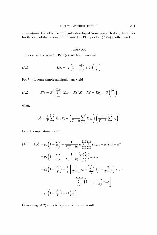
ROBUST HYPOTHESIS TESTING 871
conventional kernel estimation can be developed. Some research along these linesfor the case of sharp kernels is reported by Phillips et al. (2004) in other work.
APPENDIX
PROOF OF THEOREM 1. Part (a). We first show that
Eγh = γh
(1 − |h|
T
)+ O
( |h|T
)(A.1)
For h ≥ 0, some simple manipulations yield
Eγh = E1
T
T−h∑t=1
(Xt+h − X
)(Xt − X)′ = Eγ 0
h + O( |h|
T
)(A.2)
where
γ 0h = 1
T
T−h∑t=1
Xt+h X′t −
(1
T − h
T−h∑s=1
Xs+h
) (1
T − h
T−h∑s=1
Xs
)′
Direct computation leads to
Eγ 0h = γh
(1 − h
T
)− 1
T(T − h)E
T−h∑t=1
T−h∑s=1
(Xs+h − μ) (Xt − μ)′
= γh
(1 − h
T
)− 1
T(T − h)
T−h∑t=1
T−h∑s=1
γs+h−t
= γh
(1 − |h|
T
)− 1
T
[1
T − hγh +
T−h−1∑τ=1
(1 − τ
T − h
)γ−τ−h
+T−h−1∑
τ=1
(1 − τ
T − h
)γτ−h
]
= γh
(1 − |h|
T
)+ O
(1
T
)
(A.3)
Combining (A.2) and (A.3) gives the desired result.
872 PHILLIPS, SUN, AND JIN
Similarly, we can show that (A.1) holds for h < 0. Using (A.1), we have
T2
ρE( fXX(0) − fXX(0))
= 1
2π
T2
ρ
T−1∑h=−T+1
kρ
(hT
) (1 − |h|
T
)γh − T2
ρ
1
2π
∞∑−∞
γh
+ O
(T3
ρ
1
T
T−1∑h=−T+1
|h|T
kρ
(hT
))
= 1
2π
T2
ρ
T−1∑h=−T+1
[kρ
(hT
)− 1
]γh − 1
2π
T2
ρ
T−1∑h=−T+1
kρ
(hT
) |h|T
γh
− 1
2π
T2
ρ
∑|h|≥T
γh + O
(T3
ρ
∫ 1
0
xkρ(x) dx
)
= 1
2π
T2
ρ
T−1∑h=−T+1
[kρ
(hT
)− 1
]γh − 1
2π
T2
ρ
T−1∑h=−T+1
kρ
(hT
) |h|T
γh
+ O(
1
ρ
)+ O
(T3
ρ5/2
)
(A.4)
where the last line follows because | ∑|h|≥T γh| ≤ T−2∑
|h|≥T |h2γh| and∫ 1
0xkρ(x) dx = O( 1
ρ3/2 ). The latter order of magnitude can be proved using the
Laplace approximation method. The details are similar to the proof of (A.38) inwhat follows and are omitted. We now consider the first two terms in (A.4). Thesecond term is bounded by
1
2π
T2
ρ
T−1∑h=−T+1
|h|T
|γh| = Tρ
1
2π
T−1∑h=−T+1
|h||γh| = O(
Tρ
)= o(1)(A.5)
using Assumptions 2 and 3. The first term in (A.4) can be written as
T−1∑h=−T+1
[kρ
(hT
)− 1
]γh =
T/ log T∑h=−T/ log T
[kρ
(hT
)− 1
]γh
+∑
T/ log T≤|h|<T
[kρ
(hT
)− 1
]γh
(A.6)

ROBUST HYPOTHESIS TESTING 873
Noting that∣∣∣∣∣T2
ρ
∑T/ log T≤|h|<T
[kρ
(hT
)− 1
]γh
∣∣∣∣∣ ≤ T2
ρ
∑T/ log T≤|h|<T
|γh|
≤ log2 Tρ
∑T/ log T≤|h|<T
h2 |γh| = o
(log2 T
ρ
)
and using Assumption 1(c), we obtain
T2
ρ
T−1∑h=−T+1
[kρ
(hT
)− 1
]γh = T2
ρ
T/ log T∑h=−T/ log T
[kρ
(hT
)− 1
]γh + o
(log2 T
ρ
)
=T/ log T∑
h=−T/ log T
[k
( hT
) − 1
ρh2/T2
]h2γh + o(1)
= −g∞∑
−∞h2γh(1 + o(1))
(A.7)
Combining the above results gives
limT→∞
T2
ρE( f XX(0) − fXX(0)) = −g
∞∑−∞
h2γh(A.8)
Part (b). We prove only the scalar case. The vector case follows from standardextensions. Note that
fXX(0) = 1
2π
∫ π
−π
IXX(λ)Kρ (λ) dλ(A.9)
To find the asymptotic variance of fXX(0), we can work from the following stan-dard formula (e.g., Priestley, 1981, eqn. 6.2.110 on p. 455) for the variance of aweighted periodogram estimate such as (A.9), viz.
Var{ fXX(0)} = 2 f 2XX(0)
1
T
T−1∑h=−T+1
kρ
(hT
)2
[1 + o(1)](A.10)
which follows directly from the covariance properties of the periodogram of alinear process (e.g., Priestley, 1981, p. 426).
To evaluate (A.10), we develop an asymptotic approximation of
T−1∑T−1
h=−T+1 k2ρ( h
T ). Since kρ(x) is differentiable by Assumption 1, it follows

874 PHILLIPS, SUN, AND JIN
by Euler summation that the sum can be approximated by an integralas
1
T
T−1∑h=−T+1
k2ρ
(hT
)=
∫ 1
−1
k2ρ(x) dx(1 + o(1))(A.11)
We use Laplace’s method to approximate the above integral. It follows fromAssumption 1(b) that for any δ > 0, there exists ζ > 0 such that log k(x) ≤ −ζ (δ)for |x| ≥ δ. Therefore, the contribution of the intervals δ ≤ |x| ≤ 1 satisfies
∫δ≤|x|≤1
k2ρ(x) dx =
∫δ≤|x|≤1
exp{2ρ log k(x)} dx ≤ exp[−2(ρ − 1)ζ (δ)]
∫ 1
−1
k2(x)
(A.12)
We now deal with the integral from −δ to δ. From Assumption 2(c),
k(x) = 1 − gx2 + o(x2), as x → 0 for some g > 0
we have log k(x) = −gx2 + o(x2). So, for any given ε > 0, we can determine δ > 0such that
|log k(x) + gx2| ≤ εx2, |x| ≤ δ
In consequence,∫ δ
−δ
exp[−2ρ(g + ε)x2] dx ≤∫ δ
−δ
exp 2ρ log k(x) dx ≤∫ δ
−δ
exp[−2ρ(g − ε)x2] dx
But ∫ δ
−δ
exp[−2ρ(g + ε)x2] dx =∫ ∞
−∞exp[−2ρ(g + ε)x2] dx + O(e−ρα)
=√
π√2ρ(g + ε)
+ O(e−ρα)
for some positive α that depends on δ but not ρ.Similarly, ∫ δ
−δ
exp[−2ρ(g − ε)x2] dx =√
π√2ρ(g − ε)
+ O(e−ρα)
Therefore ∫ δ
−δ
exp 2ρ log k(x) dx =(
π
2ρg
)1/2
(1 + o(1))(A.13)
ROBUST HYPOTHESIS TESTING 875
Combining (A.12) and (A.13) yields
∫ 1
−1
k2ρ(x) dx =
(π
2ρg
)1/2
(1 + o(1))(A.14)
which completes the proof of part (b).Part (c). Part (c) follows directly from parts (a) and (b). �
PROOF OF LEMMA 1. Approximating the sum by an integral, we have
Kρ(λs) = TT−1∑
h=−T+1
kρ
(hT
)eiλs h = T
∫ 1
−1
kρ(x)ei2πsxdx(1 + o(1))
= T∫ 1
−1
exp ρ(log k(x) + log cos(2πsx))(1 + o(1))
(A.15)
Using the Laplace approximation, we find that as ρ → ∞, the contribution tothe integral in (A.15), as in the proof of Theorem 1(b), comes mainly from a smallregion around x = 0, say (−δ, δ) for some arbitrarily small δ > 0. So there existsζ (δ) > 0 such that
Kρ(λs) = T∫ δ
−δ
exp{ρ[log k(x) cos(2πsx)]}(1 + o(1)) + T exp[−ρζ (δ)](1 + o(1))
= T∫ δ
−δ
eρ log[k(x)]+2πsxi dx(1 + o(1)) + T exp[−ρζ (δ)](1 + o(1))
= T∫ δ
−δ
e−ρgx2+2πsxi dx(1 + o(1)) + T exp[−ρζ (δ)](1 + o(1))
= T∫ ∞
−∞e−ρgx2+2πsxi dx(1 + o(1)) + T exp[−ρζ (δ)](1 + o(1))
= T∫ ∞
−∞e−ρg(x2+2πsxi/ρg−(πs)2/(ρg)2)−(πs)2/(ρg) + T exp[−ρζ (δ)](1 + o(1))
=√
πT√ρg
exp
(−π2s2
ρg
)(1 + o(1))
Hence,
Kρ(λs) =
⎧⎪⎪⎨⎪⎪⎩O
(T√ρ
)for s ≤ O(
√ρ)
O(
Te− π2s2ρg√ρ
)for s > O(
√ρ)
as desired. �

876 PHILLIPS, SUN, AND JIN
PROOF OF THEOREM 2. We prove the results for the scalar case; the vector case
follows without further complication. Since fXX(0) = 1T
∑T−1s=0 Kρ(λs)IXX(λs) and
T−1∑s=0
Kρ(λs) =T−1∑
h=−T+1
kρ
(hT
) T−1∑s=0
eiλs h = Tk(0) = T(A.16)
we can write the scaled estimation error as
ρ1/4{ fXX(0) − fXX(0)} = ρ1/4
T
T−1∑s=0
Kρ(λs)[IXX(λs) − fXX(0)]
= ρ1/4
T
T−1∑s=0
Kρ(λs)[IXX(λs) − fXX(λs)]
+ ρ1/4
T
T−1∑s=0
Kρ(λs)[ fXX(λs) − fXX(0)]
(A.17)
Using Lemma 1, we have
Kρ(λs) =√
πT√ρg
exp
(−π2s2
ρg
)(1 + o(1)), s = 0, 1, . . . , [T/2](A.18)
By Assumption 2, | f ′′XX(λs)| ≤ 1
2π
∑∞−∞ h2|γh|, so that
| fXX(λs) − fXX(0)| ≤(
1
2π
∞∑−∞
|h|2|γh|)
λ2s
Hence, the second term of (A.17) can be bounded as follows:
ρ1/4
T
T−1∑s=0
Kρ(λs)[ fXX(λs) − fXX(0)]
= ρ1/4
T2
[T/2]∑s=0
Kρ(λs)[ fXX(λs) − fXX(0)] = O
(ρ1/4
T
[T/2]∑s=0
|Kρ(λs)|λ2s
)
= O
(ρ1/4
T
[T/2]∑s=0
√πT√ρg
exp
(−π2s2
ρg
)λ2
s
)
= O(
ρ−1/4T−2
∫ ∞
0
exp
(−π2s2
ρg
)s2 ds
)= O(ρ−1/4T−2) = o(1)
(A.19)

ROBUST HYPOTHESIS TESTING 877
Then, by (A.17) and (A.19), we have
ρ1/4{ fXX(0) − fXX(0)} = ρ1/4
T
T−1∑s=0
Kρ(λs)(IXX(λs) − fXX(λs)) + op(1)(A.20)
In view of Assumption 2, we have Xt = C(L)εt = ∑∞j=0 Cjεt− j . The operator C(L)
has a valid spectral BN decomposition (Phillips and Solo, 1992)
C(L) = C(eiλ) + Cλ(e−iλL)(e−iλL− 1)(A.21)
where Cλ(e−iλL) = ∑∞j=0 Cλ j e−i jλLj and Cλ j = ∑∞
s= j+1 Cseisλ, leading to the rep-resentation
Xt = C(L)εt = C(eiλ)εt + e−iλελt−1 − ελt(A.22)
where
ελt = Cλ(e−iλL)εt =∞∑j=0
Cλ j e−i jλεt− j(A.23)
is stationary. The discrete Fourier transform of Xt has the correspondingrepresentation
w(λs) = 1√2πT
T∑t=1
Xt eitλs = C(eiλs )wε(λs) + 1√2πT
(ελs 0 − einλs ελs n
)= C(eiλs )wε(λs) + Op(T−1/2)
(A.24)
Thus, using the fact that
T−1∑s=0
|Kρ(λs)| = 2√
πT√ρg
[T/2]∑s=0
exp
(−π2s2
ρg
)(1 + o(1))
=√
πT√ρg
∫ ∞
−∞exp
(−π2s2
ρg
)ds(1 + o(1))
= O(T)
(A.25)

878 PHILLIPS, SUN, AND JIN
we get
ρ1/4{ fXX(0) − fXX(0)}
= ρ1/4
T
T−1∑s=0
Kρ(λs)(IXX(λs) − fXX(λs)) + op(1)
= ρ1/4
T
T−1∑s=0
Kρ(λs)(w(λs)w(λs)∗ − fXX(λs)) + op(1)
= ρ1/4
T
T−1∑s=0
Kρ(λs){[
C(eiλs )wε(λs) + Op(T−1/2)]
× [C(eiλs )wε(λs) + Op(T−1/2)
]∗ − fXX(λs)} + op(1)
= ρ1/4
T
T−1∑s=0
Kρ(λs)
[C2(1)
(Iεε(λs) − 1
2πσ 2
)]+ Op
(ρ1/4
TT
1
T1/2
)+ op(1)
= ρ1/4
T
T−1∑s=0
Kρ(λs)
[C2(1)
(Iεε(λs) − 1
2πσ 2
)]+ op(1)
(A.26)
where we have used ρ/T2 → 0. The fourth equality follows because Kρ(λs) be-comes progressively concentrated at the origin.
Let m1 = 0 and for t ≥ 2,
mt = εt
t−1∑j=1
ε j ct− j
where
c j = C2(1)
2π
ρ1/4
T2
T−1∑s=0
(Kρ(λs) cos( jλs))
Then we can write
ρ1/4
T
T−1∑s=0
Kρ(λs)
[C2(1)
(Iεε(λs) − 1
2πσ 2
)]
= 2T∑
t=1
mt + ρ1/4
TC2(1)
T−1∑s=0
Kρ(λs)1
2π
(1
T
T∑t=1
ε2t − σ 2
)
= 2T∑
t=1
mt + ρ1/4
TC2(1)
∣∣∣∣∣T−1∑s=0
Kρ(λs)
∣∣∣∣∣ Op
(1√T
)
= 2T∑
t=1
mt + op(1)
(A.27)
ROBUST HYPOTHESIS TESTING 879
By the Fourier inversion formula, we have
c j = C2(1)
2π
ρ1/4
Tkρ
(jT
)(A.28)
Hence
T∑j=1
c2j = O
(ρ1/2
T2
T∑j=1
k2ρ
(jT
))= O
(ρ1/2
T2
(π
2ρg
)1/2
T
)= O
(1
T
)(A.29)
The sequence mt depends on T via the coefficients cj and forms a zero meanmartingale difference array. Then
2T∑
t=1
mt →d N
(0,
σ 4C4(1)
2π2
(π
2g
)1/2)
= N
(0, 2 f 2
XX(0)
(π
2g
)1/2)
by a standard martingale CLT, provided the following two sufficient conditionshold:
T∑t=1
E(m2
t
∣∣Ft−1
) − σ 4C4(1)
8π2
(π
2g
)1/2
→p 0(A.30)
whereFt−1 = σ (εt−1, εt−2, . . .) is the filtration generated by the innovations εj, and
T∑t=1
E(m4
t
) →p 0(A.31)
We now proceed to establish (A.30) and (A.31). The left-hand side of (A.30) is(σ 2
T∑t=2
t−1∑j=1
ε2j c
2t− j − σ 4C4(1)
8π2
(π
2g
)1/2)
+ σ 2T∑
t=2
∑r �= j
εrε j ct−r ct− j := I1 + I2
(A.32)
The first term, I1, is
σ 2
(T−1∑j=1
(ε2
j − σ 2) T− j∑
s=1
c2s
)+
(σ 4
T−1∑t=1
T−t∑j=1
c2j − σ 4C4(1)
8π2
(π
2g
)1/2)
:= I11 + I12
(A.33)
880 PHILLIPS, SUN, AND JIN
The mean of I11 is zero and its variance is of order
O
⎡⎣T−1∑j=1
(T− j∑s=1
c2s
)2⎤⎦ = O
⎡⎣T
(T∑
s=1
c2s
)2⎤⎦ = O
(1
T
)
using (A.29). Next, consider the second term of (A.33). We have
T−1∑j=1
T− j∑s=1
c2s = C4(1)
4π2
ρ1/2
T2
T−1∑j=1
T− j∑s=1
k2ρ
( sT
)
= C4(1)
4π2
ρ1/2
T2
T−1∑s=1
T−s∑j=1
k2ρ
( sT
)= C4(1)
4π2
ρ1/2
T
T−1∑s=1
(1 − s
T
)k2ρ
( sT
)
= C4(1)
8π2
(π
2g
)1/2
+ o(1)
Here we have used the following result, obtained by means of the Laplaceapproximation:
1
T
T−1∑s=1
(1 − s
T
)k2ρ
( sT
)= 1
2
(π
2ρg
)1/2
(1 + o(1))(A.34)
We have therefore shown that
I1 = σ 2T∑
t=2
t−1∑j=1
ε2j c
2t− j − σ 4C4(1)
8π2
(π
2g
)1/2
→p 0
So the first term of (A.32) is op(1).Now consider the second term, I2, of (A.32). I2 has mean zero and variance
O
(2
T∑p,q=2
min (p−1,q−1)∑r �= j
(cq−r cq− j cp−r cp− j )
)
= O
(2
T∑p=2
p−1∑r �= j
c2p−r c2
p− j + 4T∑
p=3
p−1∑q=2
q−1∑r �= j
(cq−r cq− j cp−r cp− j )
)(A.35)
In view of (A.29), we have
T∑p=2
p−1∑r �= j
c2p−r c2
p− j = O
⎛⎝T
(T∑
j=1
c2j
)2⎞⎠ = O
(1
T
)(A.36)

ROBUST HYPOTHESIS TESTING 881
For the second component in (A.35), we have, using (A.29) and the Cauchyinequality,
4T∑
p=3
p−1∑q=2
q−1∑r �= j
(cq−r cq− j cp−r cp− j ) ≤ 4T∑
p=3
p−1∑q=2
q−1∑r=1
c2q−r
q−1∑r=1
c2p−r
≤ 4T∑
i=1
c2i
T∑p=3
p−1∑q=2
q−1∑r=1
c2p−r ≤ 4
(T∑
i=1
c2i
) (T∑
p=3
p−1∑q=2
p−1∑r=p−q+1
c2r
)
= O
(1
T
T∑p=3
p−1∑q=2
p−1∑r=p−q+1
c2r
)= O
(1
T
T−2∑r=1
r(T − r − 1)c2r
)
= O
(ρ1/2
T3
T−2∑r=1
r(T − r − 1)kρ
( rT
))= O
(ρ1/2
∫ 1
0
x(1 − x)kρ(x) dx
)
(A.37)
We now show that
ρ1/2
∫ 1
0
x(1 − x)kρ(x) dx = o(1)(A.38)
To this end, we need the following result: If the function pρ(x) = x(1 − x)kρ(x)achieves its maximum at x∗(ρ) ∈ (0, 1), then x∗(ρ) → 0 as ρ → ∞. The result canbe proved by contradiction. Suppose for any ρ, there exists an ε > 0 and ρ0 ≥ ρ
such that x∗(ρ0) ≥ ε. Since x∗(ρ0) ≥ ε, it follows from Assumption 1 that thereexists a positive number ζ (ε) such that k(x∗(ρ0)) ≤ 1 − ζ (ε). Therefore
pρ0
(x∗(ρ0)
) ≤ x∗(ρ0)(1 − x∗(ρ0)
)[1 − ζ (ε)]ρ0 ≤ 1/4[1 − ζ (ε)]ρ0(A.39)
But for large ρ0,
pρ0(1/ρ0) = 1
ρ0
(1 − 1
ρ0
) (1 − g
ρ20
)ρ0
(1 + o(1)) = 1
ρ0
(1 + o(1))(A.40)
Hence
pρ0(1/ρ0) > pρ0
(x∗(ρ0)
)(A.41)
for large ρ0. This contradicts with the fact that x∗(ρ0) is a maximizing point. Solim x∗(ρ) must be zero. We note, in passing, that we have effectively shown thatx∗(ρ) is of order O(1/ρ). Since the function p(x) is strictly concave in a neighbor-hood of zero, x∗(ρ) is the unique maximizer for any fixed ρ.

882 PHILLIPS, SUN, AND JIN
Given that p(x) has a unique maximizer x∗, we can apply Laplace’s method to
approximate the integral∫ 1
0p(x) dx. Let
κ(x∗) = k′′(x∗)
k(x∗)− (k′(x∗))2
k2(x∗)(A.42)
then
∫ 1
0
x(1 − x)kρ(x) dx =∫ 1
0
exp[log(x) + log(1 − x) + log kρ(x)] dx
= x∗(1 − x∗)kρ(x∗)
×∫ ∞
0
exp
[−
(1
2 (x∗ − 1)2
+ 1
2(x∗)2− 1
2ρκ(x∗)
)y2
]dy(1 + o(1))
= o(
1√ρ
)
(A.43)
using limρ→∞ x∗ = 0, limρ→∞ κ(x∗) = −2g and kρ(x∗) = O(1) as ρ → ∞.Combining (A.36), (A.37), and (A.43) completes the proof of I2 →p 0. We have
therefore established condition (A.30).It remains to verify (A.31). Let A be some positive constant, then the left-hand
side of (A.31) is
μ4
T∑t=2
E
(t−1∑s=1
εsct−s
)4
≤ AT∑
t=2
E
(t−1∑s=1
t−1∑r=1
t−1∑p=1
t−1∑q=1
εsεrεpεqct−sct−r ct−pct−q
)
≤ AT∑
t=2
(T∑
s=1
c4t−s
)+ A
T∑t=2
t−1∑s=1
t−1∑r=1
c2t−sc2
t−r
≤ AT
(T∑
t=1
c2t
)2
= O(
T1
T2
)= O
(1
T
)
using (A.29), which verifies (A.31) and the CLT.
ROBUST HYPOTHESIS TESTING 883
With this construction, we therefore have
ρ1/4
TC2(1)
T−1∑s=0
Kρ(λs)
[(Iεε(λs) − 1
2πσ 2
)]
= 2T∑
t=1
mt + op(1) →d 2N
(0,
σ 4C4(1)
8π2
(π
2g
)1/2)
= N
(0,
σ 4C4(1)
2π2
(π
2g
)1/2)
= N
(0, 2
(π
2g
)1/2
f 2XX(0)
)This gives the required limit theory for the spectral estimate at the origin, viz.,
ρ1/4{ fXX(0) − fXX(0)} = ρ1/4
T
T−1∑s=0
K(λs)(IXX(λs) − fXX(λs)) + op(1)
→ d N
(0, 2
(π
2g
)1/2
f 2XX(0)
)�
PROOF OF THEOREM 3. Part (a) follows from the same arguments as in the proofof Theorem 1(a). It remains to prove part (b), as part (c) can be easily provedusing parts (a) and (b). To prove part (b), we write
fXX(ω) = 1
2π
T−1∑h=−T+1
kρ
(hT
)γhe−ihω
= 1
2π
T−1∑h=−T+1
kρ
(hT
)2π
T
T−1∑s=0
IXX(λs)ei(λs−ω)h
=T−1∑s=0
IXX(λs)ei(λs−ω)h 1
T
T−1∑h=−T+1
kρ
(hT
)
= 1
T
T−1∑s=0
K (λs − ω) IXX(λs)
As before, the variance of fXX(ω) can be calculated using a standard formula (e.g.,Priestley, 1981, eqn. 6.2.110 on p. 455):
Var{ fXX(ω)} = f 2XX(ω)
1
T
T−1∑h=−T+1
kρ
(hT
)2
[1 + o(1)]
= f 2XX(ω)
(π
2ρg
)1/2
[1 + o(1)]
(A.44)
where the last line uses (A.14). This complete the proof of part (b).

884 PHILLIPS, SUN, AND JIN
The stated result for the vector case follows directly by standard extensions(e.g., Hannan, 1970, p. 280). �
PROOF OF LEMMA 2. Approximating the sum by an integral, we have
K(λs − ω) = TT−1∑
h=−T+1
kρ
(hT
)ei(ω−λs )h = T
∫ 1
−1
kρ(x)e(ωxT−2πsx)i dx(1 + o(1))
= T∫ 1
−1
exp ρ(log k(x) + log cos(ωxT − 2πsx))(1 + o(1))
(A.45)
Proceeding as before, we approximate the integral using Laplace’s method. Forsome small δ > 0, we have
Kρ(λs) = T∫ δ
−δ
exp{ρ log[k(x) cos(ωxT − 2πsx)]}(1 + o(1))
= T∫ δ
−δ
exp{ρ log[k(x)] + (ωT − 2πs)xi} dx(1 + o(1))
= T∫ δ
−δ
exp{−ρgx2 + (ωT − 2πs)xi} dx(1 + o(1))
= T∫ ∞
−∞exp[−ρgx2 + (ωT − 2πs)xi] dx(1 + o(1))
(A.46)
Simple calculations give
Kρ(λs) = T exp[−(ωT − 2πs)2/(4ρg)]
×∫ ∞
−∞exp −ρg[x2 + (ωT − 2πs)xi/ρg − ((ωT − 2πs)2/(2ρg)2]
=√
πT√ρg
exp
(− (ωT − 2πs)2
4ρg
)(1 + o(1))
=
⎧⎪⎨⎪⎩O
(T√ρ
)for |ωT − 2πs| ≤ O(
√ρ)
O(
T√ρ
exp(− (ωT−2πs)2
4ρg
))for |ωT − 2πs| > O(
√ρ)
(A.47)
and this completes the proof. �PROOF OF THEOREM 4. As before, we consider the scalar case, as the vector case
can be proved by standard extensions. Note that
T−1∑s=0
K(λs − ω) =T−1∑
h=−T+1
kρ
(hT
) T−1∑s=0
ei(λs−ω)h = Tkρ(0) = T
and K(λs) is a real even periodic function of λs with periodicity 2π .
ROBUST HYPOTHESIS TESTING 885
Without loss of generality, we assume that T is even. Let λJ be the Fourierfrequency that is closest to ω and
Bω = {s : s = J − T/2 + 1, J − T/2, . . . , J, J + 1, . . . , J + T/2}(A.48)
Then the scaled estimation error can be written as
ρ1/4{ fXX(ω) − fXX(ω)} = ρ1/4
T
∑s∈Bω
Kρ(λs − ω)[IXX(λs) − fXX(ω)]
= ρ1/4
T
∑s∈Bω
Kρ(λs − ω)[IXX(λs) − fXX(λs)]
+ ρ1/4
T
∑s∈Bω
Kρ(λs − ω)[ fXX(λs) − fXX(ω)]
(A.49)
Using Lemma 2 and the proof similar to that for (A.20), we obtain
ρ1/4{ fXX(ω) − fXX(ω)} = ρ1/4
T
∑s∈Bω
Kρ(λs − ω)[IXX(λs) − fXX(λs)] + o(1)
(A.50)
In view of (A.24), the frequency domain BN decomposition, we have
w(λs) = C(eiλs )wε(λs) + Op(T−1/2)(A.51)
Following the same steps in (A.25), we can show that
T−1∑s=0
|Kρ(λs − ω)| = O(T)(A.52)
Plugging (A.51) into (A.50) and using (A.25), we have
ρ1/4{ fXX(ω) − fXX(ω)}
= ρ1/4
T
∑s∈Bω
Kρ(λs − ω)|C(eiw)|2[
Iεε(λs) − σ 2
2π
]
+ ρ1/4
T
∑s∈Bω
Kρ(λs − ω)(|C(eiλs )|2 − |C(eiw)|2) [
Iεε(λs) − σ 2
2π
]+ op(1)
(A.53)

886 PHILLIPS, SUN, AND JIN
where we have used ρ/T2 → 0. But the second sum in the above expression isbounded by
ρ1/4
T
∑s∈Bω
Kρ(λs − ω)|λs − ω| = op(1)(A.54)
by the smoothness of C(eiw) and Lemma 2. Hence
ρ1/4{ fXX(ω) − fXX(ω)} = ρ1/4
T|C(eiw)|2
∑s∈Bω
Kρ(λs − ω)
[Iεε(λs) − σ 2
2π
](A.55)
Let m1 = 0 and for t ≥ 2,
mt = εt
t−1∑j=1
ε j ct− j (ω)
where
c j (ω) = |C(eiw)|22π
ρ1/4
T2
∑s∈Bω
(Kρ(λs − ω) cos( jλs))
Following the same steps as in (A.27), we can write
ρ1/4
T|C(eiw)|2
∑s∈Bω
Kρ(λs − ω)
[Iεε(λs) − σ 2
2π
]= 2
T∑t=1
mt + op(1)(A.56)
Simple calculations show that
c j (ω) = |C(eiw)|24π
ρ1/4
Tkρ
(jT
)cos ω j(A.57)
Hence
T∑j=1
c2j (ω) = O
(ρ1/2
T2
T∑j=1
k2ρ
(jT
))= O
(1
T
)(A.58)
We proceed to show that
2T∑
t=1
mt →d N
(0,
σ 4|C(eiw)|44π2
(π
2g
)1/2)
= N
(0, f 2
XX(ω)
(π
2g
)1/2)
(A.59)
by verifying the following two sufficient conditions for a martingale CLT:
T∑t=1
E(m2
t
∣∣Ft−1
) − σ 4|C(eiw)|416π2
(π
2g
)1/2
→p 0(A.60)

ROBUST HYPOTHESIS TESTING 887
and
T∑t=1
E(m4
t
) →p 0(A.61)
The left-hand side of (A.60) is(σ 2
T∑t=2
t−1∑j=1
ε2j c
2t− j (ω) − σ 4C4(1)
16π2
(π
2g
)1/2)
+ σ 2T∑
t=2
∑r �= j
εrε j ct−r (ω)ct− j (ω) := I1 + I2
(A.62)
The first term, I1, is
σ 2
(T−1∑j=1
(ε2
j − σ 2) T− j∑
s=1
c2s (ω)
)+
(σ 4
T−1∑t=1
T−t∑j=1
c2j (ω) − σ 4C4(1)
16π2
(π
2g
)1/2)
:= I11 + I12
(A.63)
The mean of I11 is zero and its variance is of order
O
⎡⎣T−1∑j=1
(T− j∑s=1
c2s (ω)
)2⎤⎦ = O
⎡⎣T
(T∑
s=1
c2s (ω)
)2⎤⎦ = O
(1
T
)
using (A.58). Next, consider the second term of (A.63). We have
T−1∑j=1
T− j∑s=1
c2s (ω) = |C(eiω)|4
4π2
ρ1/2
T2
T−1∑j=1
T− j∑s=1
k2ρ
( sT
)cos2 ωs
= |C(eiω)|416π2
ρ1/2
T
T−1∑s=1
(1 − s
T
)k2ρ
( sT
)cos2 ωs
= |C(eiω)|416π2
(π
2g
)1/2
+ o(1)
(A.64)
where (A.64) follows from the approximation
1
T
T−1∑s=1
(1 − s
T
)k2ρ
( sT
)cos2 ωs =
(π
2ρg
)1/2
(1 + o(1))(A.65)
which can be proved using Laplace’s method. To save space, the details of theproof are omitted.

888 PHILLIPS, SUN, AND JIN
The above derivations therefore demonstrate that
I1 = σ 2T∑
t=2
t−1∑j=1
ε2j c
2t− j (ω) − σ 4|C(eiω)|4
16π2
(π
2g
)1/2
→p 0(A.66)
So the first term of (A.62) is op(1). Following arguments similar to the proof ofTheorem 3, we can show that I2 → p 0. In fact, since cj(ω) ≤ 1/2cj, all steps gothrough with no modifications. Similarly, condition (A.61) can be verified in thesame way.
Combining (A.55), (A.56), and (A.59) yields
ρ1/4
T|C(eiw)|2
∑s∈Bω
Kρ(λs − ω)
[Iεε(λs) − σ 2
2π
]
→d N
(0,
σ 4|C(eiω)|44π2
(π
2g
)1/2)
= N
(0,
(π
2g
)1/2
f 2XX(ω)
)(A.67)
The limit theory for the spectral estimate at ω �= 0, π now follows
ρ1/4{ fXX(ω) − fXX(ω)} →d N
(0,
(π
2g
)1/2
f 2XX(ω)
)(A.68)
as desired. �
PROOF OF THEOREM 5. Note that
fXX(ωi ) = 1
T
T−1∑s=0
K(λs − ωi )IXX(λs)
Under Assumption 2, we have
(i) Var(IXX(λs) − fXX(λs)) = 4π2δ0,λs f 2XX(λs)(1 + O(T−1/2))
(i i) Cov(IXX(λs), IXX(λτ )) = O( fXX(λs) fXX(λτ )/T), s �= τ
(A.69)
where δ0,λs = 1 + 1{λs=0,π}, and O(·) holds uniformly in λs and λτ (see 6.2.37 ofPriestley, 1981). Therefore
cov( fXX(ωi ), fXX(ω j )) =(
T−2T−1∑s=0
δs K (λs − ωi ) K(λs − ω j )
)((1 + O(T−1/2)))
+ O
(T−3
∑s �=τ
|K(λs − ωi )K(λτ − ω j )|)
(A.70)

ROBUST HYPOTHESIS TESTING 889
The second term in (A.70) is
O
{T−3
(T−1∑s=0
|K (λs − ωi ) |) (
T−1∑τ=0
|K (λτ − ω j ) |)}
= O(1/T)
using∑T−1
τ=0 |K(λτ − ω j )| = O(T). The first term in (A.70) is bounded by
O
(1
ρ
T−1∑s=0
exp
(− (ωi − λs)
2 T2
4ρg− (ω j − λs)
2 T2
4ρg
))
= O(
Tρ
∫ 2π
0
exp
(− T2
4ρg
((ωi − x)2 + (ω j − x)2
))dx
)
= O
{Tρ
∫ 2π
0
exp
[− T2
4ρg
(2
(x − ωi + ω j
2
)2
+ (ωi − ω j )2
2
)]dx
}
= O{
Tρ
exp
[− T2
8ρg(ωi − ω j )
2
] √ρ
T
}
= O{
1√ρ
exp
[− T2
8ρg(ωi − ω j )
2
]}
(A.71)
Therefore
ρ1/2cov( fXX(ωi ), fXX(ω j )) = O(ρ1/2/T) + O(
exp
[− T2
8ρg(ωi − ω j )
2
])= o(1)
(A.72)
using ρ/T2 → 0. �
PROOF OF THEOREM 6. (a) Let Xt = Xt − 1/T∑T
s=1 Xs . Simple calculationsshow that
fXX(ω) = 1
2π
T∑t=1
T∑τ=1
kρ
(t − τ
T
) (Xt e−i tω)(
Xτ e−iτω)′
(A.73)
where for a complex matrix z, z′ denotes the conjugate and transpose of z. Let
Sω(r) = 1√T
∑[Tr]
t=1 Xt e−iωt . Using summation by parts twice, we have

890 PHILLIPS, SUN, AND JIN
fXX(ω) = 1
2π
T−1∑t=1
T−1∑τ=1
Sω(t/T)Dρ
(t − τ
T
)S′
ω(τ/T)
+ 1
2πSω(1)
T−1∑τ=1
(kρ
(T − τ
T
)− kρ
(T − τ − 1
T
))S′
ω(τ/T)
+ 1
2π
T−1∑t=1
Sω(t/T)
(kρ
(t − T
T
)− kρ
(t − T + 1
T
))S′
ω(1)
+ Sω(1)S′ω(1)
(A.74)
where
Dρ
(t − τ
T
)= 2kρ
(t − τ
T
)− kρ
(t − τ − 1
T
)− kρ
(t − τ + 1
T
)(A.75)
We now consider three cases, (i) ω = 0, (ii) ω = π , and (iii) ω �= 0, π separately.First, when ω = 0, we have
S0(1) = 0, Sω(r) ⇒ �0 (W0(r) − W0(1)r) := �0V0(r)(A.76)
where V0(r) is a standard Brownian Bridge. Note that when T → ∞ such that(t/T, τ /T) → (r, s) in the Euclidean metric (‖·‖) for some r and s, we have
limT→∞
T2 DT
(t − τ
T
)= −k′′
ρ(r − s)(A.77)
Since k(·) is twice continuously differentiable, the above convergence is uniformin r and s. In other words, for any given ε > 0, there exists a positive � that isindependent of r and s such that∣∣∣∣T2 Dρ
(t − τ
T
)+ k′′
ρ(r − s)
∣∣∣∣ < ε
whenever ‖(t/T, τ/T) − (r , s)‖ < � for all (r, s) in [0, 1] × [ 0, 1]. For a proof ofthe uniformity, see Weinstock (1957).
Combining (A.74), (A.76), and (A.77), and invoking the continuous mappingtheorem, we get
fXX(0) ⇒ − 1
2π�0
∫ 1
0
∫ 1
0
k′′ρ(t − τ )V0(t)V′
0(τ ) dt dτ�′0
= 1
2π�0
∫ 1
0
∫ 1
0
kρ(t − τ ) dV0(t) dV′0(τ )�′
0
(A.78)

ROBUST HYPOTHESIS TESTING 891
where the last line follows from integration by parts. Some simple algebraicmanipulations show that the last expression is the same as (2π)−1�0
∫ ∫k∗ρ(t −
τ ) dW0(t) dW ′0(τ )�′
0 as required.Second, when ω = π , we have
Sπ (r) = 1√T
[Tr]∑t=1
(Xt − μ) e−iπ t − (X − μ)1√T
[Tr]∑t=1
e−iπ t ⇒ �π Wπ (r)(A.79)
Combining the above result with the the continuous mapping theorem leads to
fXX(π) ⇒ 1
2π�π
∫ 1
0
∫ 1
0
Wπ (t)k′′ρ(t − τ )W′
π (τ )�′π + 1
2π�π Wπ (1)Wπ (1)′�′
π
+ 1
2π�π
(∫ 1
0
kρ(1 − τ )Wπ (τ ) dτ
)W′
π (1)�′π
+ 1
2π�π Wπ (1)
(∫ 1
0
kρ(1 − τ )W′π (τ ) dτ
)�′
π
:= 1
2π�π
∫ 1
0
∫ 1
0
kρ(t − τ ) dWπ (t) dW′π (τ )�′
π
(A.80)
Finally, we consider ω �= 0, π . Note that
Sω(r) ⇒ �ω(WωR(r) + iWωI(r))(A.81)
Again using (A.74), (A.77), and the continuous mapping theorem, we get
fXX(ω) ⇒ 1
2π�ω
∫ ∫kρ(t − τ ) dWω(t) dW′
ω(τ )�′ω(A.82)
Details are omitted.(b) For ω = 0, we have
E(2π)−1�0�0�′0 = (2π)−1�0 E
∫ 1
0
∫ 1
0
k∗ρ(t, τ ) dW0(t) dW′
0(τ )�′0
= fXX(0)
∫ 1
0
k∗ρ(t, t) dt = fXX(0)
(1 −
∫ 1
0
∫ 1
0
kρ(t, τ ) dt dτ
)(A.83)
892 PHILLIPS, SUN, AND JIN
For ω �= 0, we have
E(2π)−1�ω�ω�′ω = (2π)−1�ω E
∫ 1
0
∫ 1
0
kρ(t − τ ) dWω(t) dW′ω(τ )�′
ω
= (2π)−1�ω�′ω + (2π)−1�ω�′
ω1{ω �= π} = fXX(ω)
(A.84)
(c) We prove the case when ω �= 0, π , as the proofs for the other cases are similarand simpler. Write E(vec(�ρ) vec(�ρ)′) as
E
(∫ 1
0
∫ 1
0
∫ 1
0
∫ 1
0
kρ(r, s)kρ(p, q)vec (dWω(r) dW′ω(s)) vec (dWω(p) dW′
ω(q))′)
= E
(∫ 1
0
∫ 1
0
∫ 1
0
∫ 1
0
kρ(r, s)kρ(p, q)∑
k1,k2,k3,k4∈{R,I}i#{k1,k4}(−i)#{k2,k3}
× vec(dWωk1(r) dW′
ωk2(s))vec(dWωk3
(p) dW′ωk4
(q))′)
where #A denotes the number of elements in A which are equal to “I”.Some calculations show that E(vec(dWωk1
(r) dWωk2(s))vec(dWωk3
(p) dW′ωk4
(q))′)is ⎧⎪⎪⎪⎪⎨⎪⎪⎪⎪⎩
vec(Im)vec(Im)′ dr dp1{k1=k2}1{k3=k4}, if r = s �= p = q
Im2 dr ds1{k1=k3}1{k2=k4} if r = p �= s = q
Kmm dr ds1{k1=k4}1{k2=k3} if r = q �= s = p
0, otherwise
(A.85)
Using the above result, we have
(A.86)
E (vec(�ω)vec(�ω)′)
=∑
k1,k2,k3,k4∈{R,I}i#{k1,k4}(−i)#{k2,k3}vec(Im)vec(Im)′1{k1=k2}1{k3=k4}
+∑
k1,k2,k3,k4∈{R,I}i#{k1,k4}(−i)#{k2,k3}
∫ 1
0
∫ 1
0
k2ρ(r − s) dr ds Im2 1{k1=k3}1{k2=k4}
+∑
k1,k2,k3,k4∈{R,I}i#{k1,k4}(−i)#{k2,k3}
∫ 1
0
∫ 1
0
k2ρ(r − s) dr dsKmm1{k1=k4}1{k2=k3}
= 4vec(Im)vec(Im)′ + 4
∫ 1
0
∫ 1
0
k2ρ(r − s) dr ds Im2
= 4vec(Im)vec(Im)′ + 4
∫ 1
0
∫ 1
0
k2ρ(r − s) dr ds Im2

ROBUST HYPOTHESIS TESTING 893
Hence
var(vec(�ω�ω�′ω))
= E vec(�ω�ω�′ω)vec(�ω�ω�′
ω)′ − vec(�ω E�ω�′ω)vec(�ω E�ω�′
ω)′
= E (�ω ⊗ �ω) vec(�ω)vec(�ω)′(�′ω ⊗ �′
ω) − 4vec(�ω�′ω)vec(�ω�′
ω)
= 4 (�ω ⊗ �ω) vec(Im)vec(Im)′(�′ω ⊗ �′
ω)
+ 4
∫ 1
0
∫ 1
0
k2ρ(r − s) dr ds (�ω ⊗ �ω) (�′
ω ⊗ �′ω) − 4vec(�ω�′
ω)vec(�ω�′ω)
= 4
∫ 1
0
∫ 1
0
k2ρ(r − s) dr ds (�ω ⊗ �′
ω) (�ω ⊗ �′ω)
= 4π2
∫ 1
0
∫ 1
0
k2ρ(r − s) dr ds ( fXX(ω) ⊗ fXX(ω))
(A.87)
giving the stated result. �
NOTATION
LRV Long-run varianceMSE Mean squared errorHAC Heteroskedastic and autocorrelation consistent→ d weak convergence
op(1) tends to zero in probabilityZ+ set of positive integersR (0, ∞)
Kmm m2 × m2 commutation matrix⊗ Kronecker product
vec(A) vectorization by columns[·] integer part
tr{A} trace of AR (−∞, ∞)
||A|| Euclidian norm of A
REFERENCES
ANDERSON, T., The Statistical Analysis of Time Series (New York: Wiley, 1971).ANDREWS, D. W. K., “Heteroskedasticity and Autocorrelation Consistent Covariance Ma-
trix Estimation,” Econometrica 59 (1991), 817–54.——, AND J. C. MONAHAN, “An Improved Heteroskedasticity and Autocorrelation Consis-
tent Covariance Matrix Estimator,” Econometrica 60 (1992), 953–66.CHAN, N. H., AND N. TERRIN, “Inference for Unstable Long-Memory Fractional Unit Root
Autoregressions,” Annals of Statistics 23 (1995), 1662–83.DE BRUIJN, N. G., Asymptotic Methods in Analysis (New York: Dover Publications, 1982).
894 PHILLIPS, SUN, AND JIN
DEN HAAN, W. J., AND A. LEVIN, “A Practitioners Guide to Robust Covariance MatrixEstimation,” in G. Maddala and C. Rao, eds., Handbook of Statistics: Robust Inference,Volume 15 (New York: Elsevier, 1997).
HANNAN, E. J., Multiple Time Series (New York: Wiley, 1970).HASHIMZADE, N., AND T. J. VOGELSANG, “Fixed-b Asymptotic Approximation of the Sam-
pling Behavior of Nonparametric Spectral Density Estimators,” Working Paper, De-partment of Economics, Cornell University, 2006.
JANSSON, M., “On the Error of Rejection Probability in Simple Autocorrelation RobustTests,” Econometrica 72 (2004), 937–46.
KIEFER, N. M., AND T. J. VOGELSANG, “Heteroskedasticity-Autocorrelation Robust TestingUsing Bandwidth Equal to Sample Size,” Econometric Theory 18 (2002a), 1350–66.
——, AND ——, “Heteroskedasticity-Autocorrelation Robust Standard Errors Using theBartlett Kernel without Truncation,” Econometrica 70 (2002b), 2093–5.
——, AND ——, “A New Asymptotic Theory for Heteroskedasticity-Autocorrelation Ro-bust Tests,” Econometric Theory 21 (2005), 1130–64.
LEE, C. C., AND P. C. B. PHILLIPS, “An ARMA-Prewhitened Long Run Vari-ance Estimator,” Mimeographed, Yale University, 1994 (korora.econ.yale.edu/phillips/papers/prewhite.pdf).
MAGNUS, J. R., AND H. NEUDECKER, “The Commutation Matrix: Some Properties and Ap-plications,” Annals of Statistics 7 (1979), 381–94.
NEAVE, H. R., “An Improved Formula for the Asymptotic Variance of Spectrum Estimates,”Annals of Mathematical Statistics 41 (1970), 70–7.
PARZEN, E., “On the Consistent Estimates of the Spectrum of a Stationary Time Series,”Annals of Mathematical Statistics 28 (1957), 329–48.
PHILLIPS, P. C. B., AND V. SOLO, “Asymptotics for Linear Processes,” Annals of Statistics 20(1992), 971–1001.
——, Y. SUN, AND S. JIN, “Consistent HAC Estimation and Robust Regression Testing UsingSharp Origin Kernels with No Truncation,” Cowles Foundation Discussion Paper No.1407, 2003 (http://cowles.econ.yale.edu/P/au/d phillips.htm).
——, ——, AND ——, “Improved HAR Inference Using Power Kernels without Trunca-tion,” Mimeographed, Yale University, 2004.
POLITIS, D. N., AND J. P. ROMANO, “Bias Corrected Nonparametric Spectral Density Esti-mator,” Journal of Time Series Analysis 16 (1995), 67–103.
——, AND ——, “Multivariate Density Estimation with General Flat-Top Kernels of InfiniteOrder,” Journal of Multivariate Analysis 68 (1998), 1–25.
PRIESTLEY, M. B., “Basic Considerations in the Estimation of Spectra,” Technometrics 4(1962), 551–64.
——, Spectral Analysis and Time Series (New York: Academic Press, 1981).WEINSTOCK, R., “On Continuous Differentiability,” American Mathematical Monthly 64
(1957), 492.