Spectral gap for a class of random billiards

Renato Feres∗, Hong-Kun Zhang†

Abstract

A random billiard is a random dynamical system similar to an ordinary billiard systemexcept that the standard specular reflection law is replaced with a more general stochasticoperator specifying the post-collision distribution of velocities for any given pre-collision velocity.We consider such collision operators for certain random billiards that we call billiards with

microstructure. Collisions modeled by these operators can still be thought of as elastic and timereversible. The operators are canonically determined by a second (deterministic) billiard systemthat models “microscopic roughness” on the billiard table boundary. Our main purpose here isto develop some general tools for the analysis of the collision operator of such random billiards.Among the main results, we give geometric conditions for these operators to be Hilbert-Schmidtand relate their spectrum and speed of convergence to stationary Markov chains with geometricfeatures of the microscopic billiard structure. The relationship between spectral gap and theshape of the microstructure is illustrated with several simple examples.

1 Introduction

Billiards are widely studied dynamical systems and natural model systems in classical and statisticalmechanics. In the standard set-up (see [7]) a point particle moves freely inside a domain in R

2 withpiecewise smooth boundary—the billiard table—reflecting elastically at the boundary according tothe usual law of equal angles of incidence and reflection. More generally, one may consider billiardsystems in which the reflection law is probabilistic. In this case, the particle is reflected at arandom direction after each collision, according to some probability distribution that depends ingeneral on the direction of incidence. We call systems of this kind random billiards. An ordinarydeterministic billiard is an extreme special case for which the distribution of post-collision velocities isconcentrated on the mirror image of the pre-collision velocity. Another example of random reflectionoften studied in classical kinetic theory of gases is the so-called cosine law ([13, 12]), according towhich the distribution of post-collision velocities is given by the probability measure ν defined bydν(v) = ρ(v)dS(v), where S is the area measure on the space of inward pointing unit vectors atthe collision point and ρ(v) is, up to a normalization constant, the cosine of the angle that v makeswith the inward-pointing normal to the boundary at that point. The measure ν, which will play animportant role in this paper, is often called the (Knudsen) cosine law. It turns out to be the (oftenunique) equilibrium (or invariant) scattering distribution for the types of random billiards that willbe studied here.

This paper is concerned with a special class of random billiards, which we call billiards withmicrostructure. The random reflection law for these systems is defined on the basis of a geometricmodel of “microscopic surface texture” with which the billiard particle interacts at a collision point.This microstructure, in turn, is specified by an associated deterministic billiard system on a second

∗Department of Mathematics, Washington University, Campus Box 1146, St. Louis, MO 63130†Department of Mathematics & Statistics, University of Massachusetts, Amherst, MA 01003

1

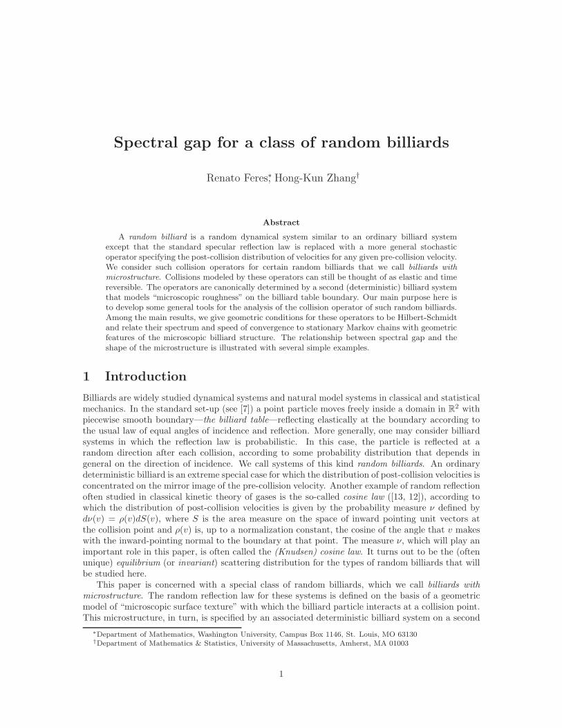
billiard table Q, referred to as the billiard cell. Heuristically, the inner surface of the walls of thefirst (“macroscopic”) billiard table is imagined as “microscopically rough” (see Figure 1), and thebilliard cell Q is the motif of a periodic pattern defining this microscopic roughness. Throughoutthe paper, we suppose that Q ⊂ R

2 has piecewise smooth boundary of finite total length, havingone special boundary segment Γ0, which is a flat segment. Without loss of generality, we identifyΓ0 with the interval [0, 1]. Further assumptions on Q will be stated later.

Figure 1: Heuristic description of a billiard with microstructure. The microstructure is periodic and thelength scales of the “macro-” and “micro-” billiard tables (the channel and a cell of the periodic structure,respectively) are not comparable, so the precise position at which a particle enters a cell Q is not defined.This position is thus assumed to be a uniformly distributed random variable. The particular Q shown hereand in Figure 2 is arbitrary.

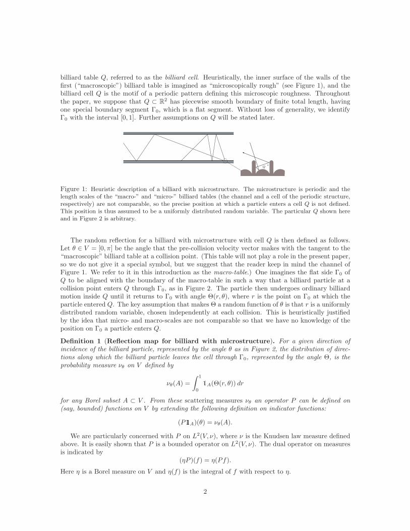
The random reflection for a billiard with microstructure with cell Q is then defined as follows.Let θ ∈ V = [0, π] be the angle that the pre-collision velocity vector makes with the tangent to the“macroscopic” billiard table at a collision point. (This table will not play a role in the present paper,so we do not give it a special symbol, but we suggest that the reader keep in mind the channel ofFigure 1. We refer to it in this introduction as the macro-table.) One imagines the flat side Γ0 ofQ to be aligned with the boundary of the macro-table in such a way that a billiard particle at acollision point enters Q through Γ0, as in Figure 2. The particle then undergoes ordinary billiardmotion inside Q until it returns to Γ0 with angle Θ(r, θ), where r is the point on Γ0 at which theparticle entered Q. The key assumption that makes Θ a random function of θ is that r is a uniformlydistributed random variable, chosen independently at each collision. This is heuristically justifiedby the idea that micro- and macro-scales are not comparable so that we have no knowledge of theposition on Γ0 a particle enters Q.

Definition 1 (Reflection map for billiard with microstructure). For a given direction ofincidence of the billiard particle, represented by the angle θ as in Figure 2, the distribution of direc-tions along which the billiard particle leaves the cell through Γ0, represented by the angle Θ, is theprobability measure νθ on V defined by

νθ(A) =

∫ 1

0

1A(Θ(r, θ)) dr

for any Borel subset A ⊂ V . From these scattering measures νθ an operator P can be defined on(say, bounded) functions on V by extending the following definition on indicator functions:

(P1A)(θ) = νθ(A).

We are particularly concerned with P on L2(V, ν), where ν is the Knudsen law measure definedabove. It is easily shown that P is a bounded operator on L2(V, ν). The dual operator on measuresis indicated by

(ηP )(f) = η(Pf).

Here η is a Borel measure on V and η(f) is the integral of f with respect to η.

2

The random reflection law of a billiard with microstructure has a number of special features: (1) itdepends canonically on a choice of billiard cell, leading naturally to the problem of relating the shapeof the cell and properties of the associated Markov chain; (2) reflection off a billiard microstructureis still “elastic” in a certain sense. For example, the angle component of the invariant measure ofdeterministic billiards (i.e., the measure ν), is a stationary distribution of directions for the collisionoperator (or Markov operator) P , and it is typically unique; (3) the Markov chain comprising thesequence of random collision angles with initial distribution ν (say, in the channel shown in Figure1) is time reversible and the process satisfies detailed balance. As shown later, this implies for Qbilaterally symmetric that P is a self-adjoint bounded (of norm 1) operator on L2(V, ν).

Figure 2: Angle convention for the pre- and post-collision vectors of two successive collision events. For ourpresent purposes it is useful to think that the entire system consists of a single billiard cell Q, and that thesegment Γ0 on the boundary of Q, which is identified with [0, 1], is also reflecting as in an ordinary billiard.But at each collision with Γ0 the particle jumps instantaneously to another point of Γ0 (indicated by s on theright-hand cell), chosen randomly and independently of the other variables, and continues its motion insideQ. From this point of view both Θ and θ measure angles from the horizontal segment counterclockwise.

The main focus of this paper is on properties of P , on the associated Markov chains, and onthe relationship they have with the shape of the billiard cell. We develop tools that can help inthe general analysis of these operators, and apply these tools to estimate spectral gap and rate ofdecay of correlations under certain geometric conditions. One geometric feature of Q that affectsthe spectral properties of P in an important way is the curvature of the part of the boundary of Qadjacent to the flat side Γ0, hence the part that is most exposed to collisions with the billiard particle.By the (normalized) curvature we mean the reciprocal of the ratio of the radius of curvature of thearc by the length of Γ0. Note that P is not affected by homotheties of Q so geometric quantities ofinterest are all dimension-free ratios.

It turns out that the methods for studying the effect of curvature on P are very different whenthe curvature is large and when it is small. For a first look at the case of small curvature see [17],where much sharper results are obtained for a special family of billiards using a perturbative method.Here we are mainly interested in large values of the curvature.

This paper is the basis for investigating other problems of interest, such as obtaining diffusioncharacteristics of the random billiard system in channels (as in Figure 1). The diffusion problem inchannels is something that will be taken up in a subsequent paper. Thus the concern here is withthe billiard cell Q and the operator P , and not with the random billiard itself. With this in mind,it is convenient to describe our random billiard in a slightly different, but equivalent, way that onlyrefers to Q, as follows: The billiard particle moves inside Q as in an ordinary billiard system, untilit collides with Γ0, at which time the particle jumps instantaneously to a randomly chosen point onΓ0 and continues inside Q after standard reflection on Γ0.

Many of the more general facts proven in the subsequent sections (concerning the stationarydistribution and basic operator properties of P ) can be shown to hold for much more realisticmodels of surface roughness, including random media in dimension 3. In order to keep definitionsto a minimum we only consider for now the periodic case in dimension 2 as described above.

3

1.1 Main results

We describe here the main results concerning convergence to the stationary measure and spectralgap. More results of general interest are given later in the paper.

The following are standing assumptions: Q ⊂ R2 is a domain with piecewise smooth boundary

of finite length and a finite number of smooth boundary segments. The smooth segments of theboundary of Q are grouped into four sets: ∂Q = Γ0 ∪ Γ1 ∪ Γ2 ∪ Γ3, where Γ0 is a flat segment, Γ1

and Γ2 are dispersing segments adjacent to Γ0, whose curvatures are bounded away from 0, and Γ3

is the union of all the remaining segments. The segments Γ1 and Γ2 are allowed to intersect Γ0 (ateach of the endpoints of Γ0) at angles in [0, π/2). Without loss of generality, we often assume thatΓ0 has length 1 and identify it with the interval I = [0, 1]. It is convenient, but not essential, to alsoassume that Q is bilaterally symmetric, i.e., invariant under reflection on the line passing throughthe middle of Γ0 and perpendicular to it.

Figure 3: Examples of billiard cells for which most of the main theorems apply. The simpler cell on the leftwill be used for illustration purposes at a few places in the paper. For the cell on the right, Γ3 consists ofthe entire contour above the (shorter) dashed line.

Let λ be the Lebesgue measure on the unit interval I and M := I × V . The return billiardmap is defined for a.e. point of M and it leaves invariant the probability measure µ := λ ⊗ ν. LetΨθ(r) := Θ(r, θ), where Θ is as shown in Figure 2. Each coordinate slice I × θ is split by thesingular set of the return map (see Section 2.1) into at most countably many intervals Wθ,j and oneach such interval Ψθ,j := Ψθ|Wθ,j

is a diffeomorphism onto its image Vθ,j ⊂ V . Now define theexpansion factor Λθ,j on Vθ,j by

Λθ,j(ϕ) :=1

2

∣∣∣Ψ′θ(Ψ

−1θ,j(ϕ))

∣∣∣ sinϕ.

The following simple fact is a special case of the main observation of Section 2.6.

Proposition 1. If Ψ′θ(r) 6= 0 for µ-a.e. (r, θ) in M , then P is an integral operator on L2(V, ν) with

integral kernel

ω(θ, ϕ) :=∑

j

1Vθ,j(ϕ)/Λθ,j(ϕ).

When P is an integral operator, then P is a compact operator if its integral kernel ω lies inL2(V × V, ν ⊗ ν). A general criterion for compactness was given in [14].

Assumption 1. In addition to the standing assumptions suppose that Γ1 and Γ2 are arcs of circleof equal radius, subtended angle π/2 (quarter circles), both tangent to Γ0 at each of the endpointsof Γ0, and the straight line connecting the endpoints of Γ1 and Γ2 not in Γ0 separates Γ3 from Γ0.(See the billiard cells of Figure 3.)

This assumption can likely be relaxed without significantly changing the conclusions of the belowtheorems, but the cost would be to add technical complications that we wish to avoid for the sakeof clarity. For example, in some of the case studies discussed in Section 1.2, Q contains verticalline segments in positions that are not strictly permitted by Assumption 1, although it would takerelatively small changes in the analysis so as to allow this feature.

4

The spectral gap of P and of other stochastic operators to appear shortly, is defined here as1 minus the spectral radius of the restriction of P to the orthogonal complement of the constantfunctions in L2(V, ν). The operator will be called quasi-compact if its essential spectral radius isstrictly less than the spectral radius (which is equal to 1).

By curvature, in particular the constant curvature K of Γ1 and Γ2 under Assumption 1, it isalways understood the ratio of the length of Γ0 (typically taken without loss of generality to be 1)by a radius of curvature.

Theorem 1. Under Assumption 1, the collision operator P is quasi-compact and its spectral gap γsatisfies

γ ≥√

2 − ǫ

Kfor any ǫ > 0 and all sufficiently large curvature K. There are examples (below) for which γ ≤ 2/K.

Most of the analysis of P involves another operator, P1, that captures the isolated effect of thescattering bumps Γ1 and Γ2. This is based on a general method that we refer to as conditioning,which can be used more generally to extricate the effect on P of various geometric features of Q.Conditioning is used later in several instances for a number of different purposes.

In particular, focusing attention on the bumps leads to a P1 defined roughly as follows. LetM1 bethe subset of M consisting of initial conditions whose billiard trajectories only undergo one collisionwith the boundary of Q before returning to Γ0, and this collision is with Γ1 or Γ2. Then define P1 asP conditional on the event M1. It turns out that P1 is a bounded self-adjoint operator on L2(V, ν1)of norm 1, where ν1 is the unique stationary measure for P1, and is absolutely continuous withrespect to ν. Similarly define P2 from M2 = M \M1. Define αi(θ) = λ(Mi,θ), the Lebesgue measureof the intersection Mi,θ of Mi and the slice [0, 1] × θ, and let as before µ denote the probabilitymeasure on M invariant under the return billiard map. We refer to M1,M2 as the special partitionof M . Other partitions will come up in the course of the paper. A common feature of many of themis that elements of the partition are cut out by singular curves of the return billiard map to M .

Theorem 2. Let M1,M2 be the special partition and Ii : L2(V, ν) → L2(V, νi) the inclusion operator.This is a bounded isomorphism with bounded inverse. Then P decomposes as

P = µ(M1)I∗1P1I1 + µ(M2)I

∗2P2I2.

and the following hold:

1. For any ǫ > 0 and all sufficiently big K

‖µ(M2)I∗2P2I2‖2 ≤ 1 − (

√2 − ǫ)/K.

2. P1 is a Hilbert-Schmidt operator of norm 1 whose spectral gap satisfies

γ1 ≥ 1 −O(K−1/N )

for some positive integer N , and all K sufficiently big. (More detailed information is obtainedin the course of the proof.) Therefore, the spectral gap of P1 approaches its maximum allowedvalue as the normalized curvature becomes very big.

3. The stochastic operator P1 is geometrically ergodic: If ν1 denotes its invariant probabilitymeasure (described explicitly later) and η is any probability measure not having atoms at 0 andπ then, for some positive constant Cη,

‖ηPm1 − ν1‖TV ≤ Cηrm/3

for all positive integers m, where r = 1 − (2 −√

2)(1 − O(1/K)). P1 restricted to L∞(V, ν1)satisfies exponential decay of correlations with the same rate r1/3.

5

Our results concerning P have parallels with certain results about chaotic billiard maps in thedeterministic setting. Chaotic billiards have been studied by Sinai, Bunimovich, Chernov [19, 1, 3, 4]and many others, who have established ergodicity and strong statistical properties under very generalassumptions on the boundary of the table [6, 18, 21, 22]. But under our assumptions on Q thedeterministic billiard map need not have as strong statistical properties as we show for P . Forexample, we allow Γ3 to contain mushroom-shaped curves (see the right-hand side of Figure 3),which is shown in [2] to produce invariant islands in the phase space of the deterministic billiard. Infact, under our assumptions on Q yielding positive spectral gap for P , the deterministic billiard mayhave arbitrarily slow decay of correlations and not even be ergodic. Compare with [9, 18, 10, 11].Of course, our Markov operators are in many respects much simpler than similar objects consideredin deterministic chaotic billiards (we are, in effect, looking at random 1-dimensional systems), yetthey are canonically associated to such billiards. Thus we believe that our operator P is a naturalobject of study which, on one hand, captures some interesting aspects of the chaotic dynamicsof billiard maps while being, on the other hand, technically much simpler and amenable to moreexplicit analysis compared to related operators of the deterministic theory, such as transfer operators.Another context in which our collision operators may be of interest is in the theory of the Boltzmannequation, where they naturally define boundary conditions that model gas-surface interaction. See,for example, [5].

Further facts of general interest concerning P are described in the subsequent sections, partic-ularly Section 2. The already mentioned technique of conditioning, in particular, provides usefulinformation about P , such as a Lebesgue decomposition (Proposition 7) giving conditions for P to bean integral operator. The technique can be used much more broadly for the purpose of investigatinghow different geometric features of the billiard cell Q affect the spectral theory of P . We finish thisintroduction with some examples that illustrate this point and other properties.

1.2 Examples

We now describe a few examples and compare some of the analytical conclusions with numericalobservations. The numerical experiments were based on finite rank approximations of the collisionoperators based on simulation of the billiard dynamics.

Figure 4: Three examples of microstructures to illustrate the idea of conditioning. Each shows a billiardcell and parts of adjacent cells. The first on the left consists of simple bumps. The dashed vertical lines areimmaterial in this case. The second example adds vertical walls of height h to the first example, and in thethird example the vertical walls have thickness δ. The explanations are in the text.

A useful technique employed throughout the paper is to consider in addition to P other operatorsobtained by making P conditional on the event that trajectories satisfy a given property, thusallowing one to focus attention on isolated geometric features. The main purpose of this subsectionis to illustrate the use of this idea in estimating spectral gap. The examples all involve relativelysimple shapes derived from circular bumps and straight walls.

Consider the billiard cells of Figure 4. (In this discussion, the partition M1,M2 and the operatorsP1, P2 are not those of Theorem 2. The general definition of these and related concepts are found inSection 2.) The reflection operator associated to the cell on the right will be denoted Ph,δ. This cellconsists of the region containing the circular bump and one entire wall. We denote the operator for

6

the middle cell by Ph,0, and the operator for the cell on the left by P . A common geometric featureof all three cells, and the only feature of that on the left, is the circular bump. We wish to describePh,δ and Ph,0 in terms of P .

We first relate Ph,δ and Ph,0 for a positive δ. Let M1 be the set of initial conditions in Mcorresponding to trajectories that enter the region of the bump, i.e., that do not hit the lower flatbottom of the wall. Now form the partition M1,M2 = M \M1 of M . Then α1 (see the generaldefinition in Subsection 2.1) is constant (independent of θ) and equal to l/(l+ δ), and α1 = µ(M1).Conditional on M1, reflection is described by Ph,0, and conditional on M2 reflection (in terms of ourangles convention) is given by the identity operator. Therefore,

Ph,δ =l

l + δPh,0 +

δ

l + δI.

Since P1 := Ph,0 and P2 := I commute and the αi are constants, any question concerning thespectrum of Ph,δ immediately reduces to understanding the same question for Ph,0.

0.1 0.2 0.3 0.4 0.5

0.2

0.25

0.3

0.35

0.4

0.45

0.5

height of vertical wall

spec

tral

gap

Figure 5: Numerically obtained spectral gap for the example of the middle microstructure of Figure 4 as afunction of wall height. The circular bump used is such that the slope of its tangent line at a corner pointis 0.4. The length l is set to 1 and the horizontal axis represents h. Observe that the gap grows very fastfor small h and suddenly reaches a plateau when h is nearly the height of the circular bump itself.

For example, the spectral gaps of Ph,δ and Ph,0 are clearly related by

γ(Ph,δ) =l

l + δγ(Ph,0),

and the factor multiplying γ(Ph,0) can be expressed in terms of the normalized curvature of thecircular bumps approximately as a constant times 1/K. Observe that K tends to infinity as l/δtends to 0 as one expects from Theorem 1. (Assumption 1 does not, strictly, hold in this case,but it would be easy to extend the theorem so as to apply to this example.) We note in passingthe similarity between the operator for this class of billiard cells and the well-known Maxwell-Smoluchowsky boundary operator for the Boltzmann equation describing a gas contained by solidwalls. The latter operator has the form (1 − a)Pν + aI, where a is the slip probability and Pνis the rank-one operator that maps any probability measure to the stationary (Knudsen’s cosine)distribution ν.

We now wish similarly to reduce Ph,0 to P and understand the effect of adding the vertical wallsto the simpler cell on the left side of the figure. In this case, let M1 consist of the initial conditionsfor billiard trajectories in the cell corresponding to Ph,0 for which the exit angle is exactly the sameas it would be for trajectories entering the cell on the left with the same conditions. Thus conditionalon M1, Ph,0 can be replaced with P . And conditional on the complementary event M2 := M \M1,

7

the operator Ph,0 is equal to PJ , where J is the unitary involution on functions of the angle inducedby the map θ 7→ π− θ. It will be seen later that P and J commute. (See Subsection 2.4.) Note thatfor large values of h one expects α1 and α2 to be close to 1/2 for most angles, although the analyticexpression of these probabilities may be difficulty to describe explicitly.

Thus we have

(1.1) Ph,0 = α1P + (1 − α1)PJ.

We can derive from this the following observation about the spectral gap of Ph,0. We say thatthe billiard cell associated to P (which may be arbitrary in this discussion) satisfies the second-oddcondition if there exists a simple eigenvalue λ of P with eigenfunction ψ such that (1) ψ is J-odd,i.e., Jψ = −ψ, and (2) the spectral radius of P restricted to the orthogonal complement of thespan of 1, ψ in L2(V, ν) (where ν is the probability measure invariant under P ) is strictly lessthan |λ|. Although we do not offer a characterization of this property here, we note that [17] givesstrong indication that the particular P illustrated in the above figure satisfies it, and our numericalcalculations show that the property holds very generally. See Figure 5, which corresponds to themiddle microstructure of Figure 4. Under this condition we have the following.

Proposition 2. If P satisfies the second-odd condition, then by adding walls of height h > 0 to thecells defining P , the spectral gap of Ph,0 cannot be smaller than the gap of P .

Proof. If ψ is an eigenfunction of P associated to a simple eigenvalue λ, then ψ is either J-even orJ-odd. It ψ is J-even, then it is easily checked using 1.1 that ψ is an eigenfunction for Ph,0 withthe same eigenvalue, for all values of h. On the other hand, if ψ is J-odd (the relevant case for theproposition), then Ph,0ψ = λ(2α1 − 1)ψ. Since the norm of the multiplication operator by 2α1 − 1is no greater than 1, we have the claim. Note that this norm can decrease to 0 as h grows and α1

is expected to approach 1/2.

0 0.2 0.4 0.6 0.8 1 1.2 1.4 1.6 1.80

0.2

0.4

0.6

0.8

1

Curvature K

Spe

ctra

l gap

γ

Figure 6: Spectral gap γ(K) (solid line) and 1

3K2 (dashed line) for the circular bumps cells (left-hand side

of Figure 4), for small values of K. By this approximation, in the experiment of Figure 5 for which K is

approximately 0.7, we have γ(K) slightly below 0.2

A study of the microstructure on the left-hand side of Figure 4 for small values of the normalizedcurvature was done in [17] using very different techniques and more detailed information was obtainedabout the spectrum of the Markov operator. Figure 6 contains one observation from that paperregarding the dependence of the spectral gap γ on the normalized curvature for that family ofcircular bumps. The asymptotic relation γ(K) ∼ K2/3 for small K was explained there.

8

Consider now the family of cells shown in Figure 7. The first two from left to right are not(bilaterally) symmetric. If P+ and P− denote the respective Markov operators, then

P ∗− = P+ = JP−J,

where J is the unitary involution introduced above. These two operators are associated to that ofthe fourth cell of Figure 7 conditional on the events that the trajectories enter into the left or theright side of the cell. Therefore,

P0 =1

2(P+ + JP+J) ,

which is now self-adjoint (and, by our theorem, compact).The relationship between the operators associated to the second and third cells in Figure 7 has

already been discussed. It was noted above that the addition of the wall should not cause thespectral gap to decrease. In the present example there is actually little change in the gap. Theobtained numerical values are: 0.694 for the spectral gap of P0 and 0.697 for the spectral gap of P1.

Figure 7: Some billiard cells discussed in the text with their respective collision operators.

Note that P1 can be written in terms of P0 as

P1 = αeP0 + (1 − αe)P0J

where αe(θ) = λ (Me ∩ (I × θ)) and Me is the event that the outgoing direction is the same forP0 and P1. So

Me = M0 ∪M2 ∪M4 ∪ · · ·where Mn is the set of initial conditions of trajectories that bounce off the vertical wall exactly ntimes before reemerging from the cell.

The left-most cell in Figure 7 can be analyzed in terms of P1 and P2, the latter being therectangular cell second to last in that figure. We have

P2 = αI + (1 − α)J

where θ 7→ α(θ) is the probability that a billiard trajectory reemerges from the rectangular cell withthe outgoing angle equal to the incoming angle. By our angle conventions, this amounts to specularreflection and is represented by the identity operator. It is not difficulty to show (by a standard“unfolding” argument) that α is given as follows: Let l = 1 − 2/K be the length of the entry/exitsegment, h = 1/K the height of the rectangular cell, and write

2h

l tan θ= k(θ) + s(θ), α(θ) =

s(θ) if k is odd

1 − s(θ) if k is even

where k(θ) ∈ Z is the integer part of 2h/(l tan θ) and s(θ) ∈ [0, 1) is its fractional part. It is clearthat the function αK = α converges uniformly to 1 as K tends to ∞ on any compact subset of (0, π).Therefore, P2 approaches the identity in the strong operator topology of L2(V, ν). Now, changing

9

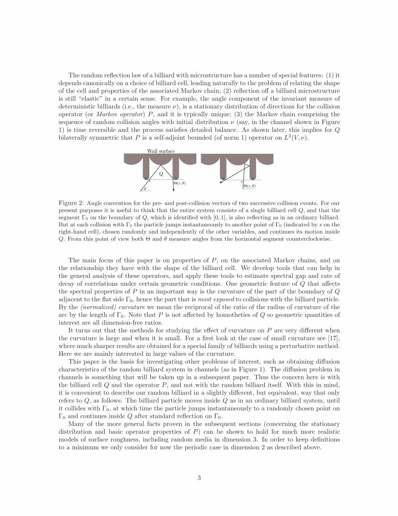
notations slightly to make explicit the dependence on the normalized curvature K, the operatorPK = P can be expressed in terms of the previous ones:

PK =2

KP1 +

(1 − 2

K

)P2,K

where αK := α = k + s is the function that enters in the expression of P2,K = P2.

4 10 16 22

0.1

0.2

0.3

0.4

Normalized curvature K

spec

tral

gap

Figure 8: Spectral gap of the operator associated to the cell obtained by taking away from the right-mostcell of Figure 7 the vertical walls. The solid line is the graph of 2/K and the values marked with an asteriskare numerically obtained.

We observe that essentially the same proof used for part (2) of Theorem 2 gives that P1 is aHilbert-Schmidt operator.

Proposition 3. Let PK be the Markov operator of the right-most billiard cell in Figure 7. Then thespectral gap of PK is bounded above by 2/K.

Proof. Let L2(V, ν) = H+ ⊕ H− be the orthogonal decomposition of the Hilbert space into theeigenspaces of J . The compact operator P1 commutes with J , so P1 has a basis of eigenfunctionsadapted to the orthogonal splitting. If φeven is any eigenfunction of P1 in H+ with eigenvalue λeven,then PKφeven = (1 − (2/K)(1 − λeven))φeven, so the spectral gap of PK is no greater than 2/K.

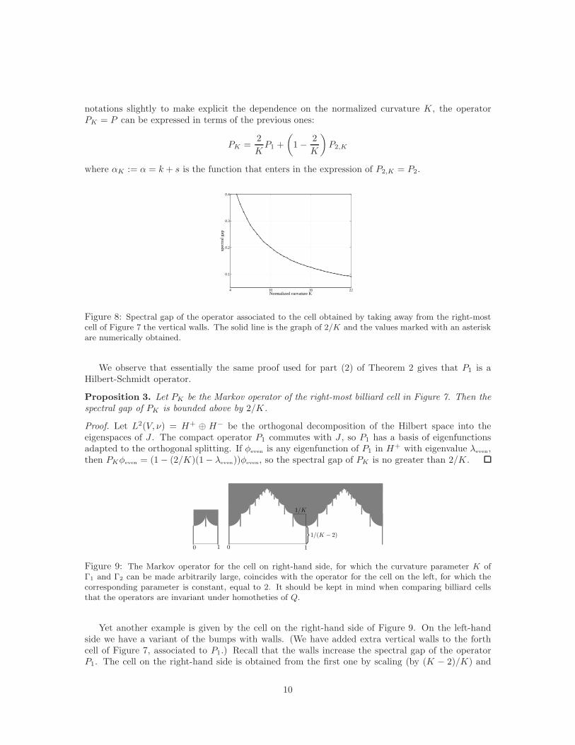
Figure 9: The Markov operator for the cell on right-hand side, for which the curvature parameter K ofΓ1 and Γ2 can be made arbitrarily large, coincides with the operator for the cell on the left, for which thecorresponding parameter is constant, equal to 2. It should be kept in mind when comparing billiard cellsthat the operators are invariant under homotheties of Q.

Yet another example is given by the cell on the right-hand side of Figure 9. On the left-handside we have a variant of the bumps with walls. (We have added extra vertical walls to the forthcell of Figure 7, associated to P1.) Recall that the walls increase the spectral gap of the operatorP1. The cell on the right-hand side is obtained from the first one by scaling (by (K − 2)/K) and

10

nesting. It is not difficulty to see, using the idea of conditioning, that the Markov operator P of thecell on the right and the operator P1 of the cell on the left satisfy the recursive relation

(1.2) P =2

KP1 +

K − 2

KP.

Proposition 4. The two billiard cells depicted in Figure 9 have the same associated Markov operator.In particular, the spectral gap of the cell on the right-hand side of the figure does not depend on K.

Proof. This follows immediately from the recursive relation 1.2 involving P and P1.

Figure 10: Example of a multi-parameter family of cells for which spectral gap can change very abruptlyas a function of one of the parameters. See Figure 11.

There are many other geometric features one would like to explore and many interesting numericalobservations for which we cannot as yet provide an analytical explanation. There are also manyissues of a general nature to understand; for example, under what conditions is the spectral gap acontinuous function of the geometric parameters?

−0.5 0 0.50.1

0.2

0.3

distance between bumps, h

spec

tral

gap

Figure 11: Spectral gap as a function of the relative height of the short and long bumps for the cell ofFigure 10. The sharp transition roughly occurs at h = 0, when the two bumps are nearly at the same height.

The example of Figure 10 shows, numerically, that the spectral gap can change very quickly forcertain values of a parameter. The figure depicts a billiard cell in which there are two competingcurvature constants associated to two arc segments. They are placed at different positions specifiedby another (relative height) parameter h so that one or the other is more exposed to collision. Biggercurvature is expected to cause bigger spectral gap, so we should see a transition from relatively largeto relatively small gap as the height parameter changes from large to small (as in figure Figure 10.)The graph of Figure 11 shows that the expected transition is very sharp. One would like to obtainestimates that better quantify and explain phenomena of this kind.

11

Another among many questions of interest to us concerns the maximum size of the spectral gap.Is it possible to find billiard cells for which γ(P ) is arbitrarily close to the upper bound 1? Thelargest value we have obtained so far in our numerical experiments is 0.91.

2 The random billiard Markov chain

This section describes in more detail the Markov process determined by P and how it relates to thereturn billiard map to the wall Γ0.

2.1 The reduced billiard map

We review some basic facts concerning billiard maps. For details, see [7]. Let Γ = ∂Q =⋃i Γi be

the decomposition of the boundary of the billiard cell Q into its smooth component curves, or walls.The boundary is oriented so that Q lies to the left of each Γj . Let n be the unit normal vector field

on each Γj pointing into Q. Define the collision space M =⋃i Mi, where Mi is the set of pairs

(q, v) ∈ Γj such that 〈v,n(q)〉 ≥ 0. With a little abuse of notation let ∂M denote the union of theboundaries of the Mi and M = M \ ∂M. We denote by F : M → M the billiard map, whose precisedefinition can be found in [7]. If x = (q, v) ∈ M and the first intersection q′ of the ray q+ tv, t > 0,with ∂Q is not a corner point of ∂Q (i.e., an endpoint of a wall) nor is v tangent to ∂Q at q′ (grazingcollision), then the billiard map is simply F(x) = (q′, v′), where v′ is the orthogonal reflection of von the tangent space to ∂Q at q′. Also define S0 = ∂M, S±1 = S0 ∪ x ∈ M : F±1(x) /∈ M and,inductively,

S±(m+1) = S±m ∪ F∓m(S±m).

It can be shown that M\S±1 are open sets and that F : M\S1 → M\S−1 is a smooth diffeomorphism.

We refer to S±1 as the singularity set of F±1. The set M := M \ ∪∞j=−∞Sj is a dense Gδ-subset

of M of full Lebesgue measure on which F and all its positive and negative iterates are smooth.Furthermore, F leaves invariant a smooth probability measure on M.

Figure 12: A qualitative description of the singular sets S+ and S− of the return map T to M . The shadedregion indicates parts of the singular sets which will not enter into the analysis. If the incoming direction ofthe billiard particle is small enough (close to 0 or π), the shaded regions are not seen.

Let M = M0 be the subset of M consisting of (q, v) such that q ∈ Γ0. We denote by µ theprobability measure on M obtained by restricting to M (and normalizing) the invariant measure

on M. By Poincare recurrence, there is a subset E0 ⊂ M ∩ M of full µ-measure such that billiardorbits starting in E0 return to M and are non-singular. Since these orbits return to M in a finitenumber of steps, there is an open neighborhood in M of each x ∈ E0 all of whose points return to

12

M in the same number of steps as the orbit of x, and the return map on this open set is smooth.Therefore, E0 is actually an open subset of M of full measure on which the first return map to Mis well-defined and smooth. We can enlarge E0 to a set E that also includes singular orbits thateventually still return to M ; i.e., possibly grazing orbits that do not get trapped in Q and do nothit a corner point along the way. Note that, due to the standing assumptions on ∂Q (specifically,that Γ1 and Γ2 are tangent to Γ0 and have positive curvature bounded away from 0), the first returnmap T : E →M is defined for all vectors that arrive at Γ0 at angles close enough to 0 or π, and E0

contains all vectors based at the two endpoints of Γ0.Denoting by S1 the singular set of T and by S−1 the singular set of T−1 (these are compact

subsets of M), then T : M \ S1 →M \ S−1 is a smooth diffeomorphism. A more precise descriptionof S±1, at least for vectors that are relatively close to tangent vectors on Γ0, will be given later.For simplicity, we often refer to T as a map on M itself. We call T the reduced billiard map on M .Notice that the probability measure µ on M defined as the (normalized) restriction to M of theLiouville measure is T -invariant.

Coordinates on M and on M can be introduced by representing the base-point of a vector bythe arc length parameter r (increasing in the sense defined by the orientation of Γ) and the angleθ that the vector makes with the positive tangent unit vector to the boundary. In particular, weparametrize M by identifying it with I × [0, π]. This definition of θ is different than the commonchoice (for example, [7]) of measuring the angle from n, but it is more convenient for our purposes.In this set of coordinates the measure µ has the form µ = λ ⊗ ν, where λ is the Lebesgue measureon [0, 1] and dν(θ) = 1

2 sin(θ) dθ.

2.2 Some operators associated to T

Summarizing basic notation: V = [0, π], I = [0, 1], M = I × V , π2 : M → V is the coordinateprojection, and ν is the probability measure on V such that dν = 1

2 sin(θ)dθ. Let P be the operatoron L∞(V, ν) defined by

(Pf)(θ) =

∫

I

f(π2 T (s, θ)) ds.

If A is a measurable subset of V , then

P (A|θ) := (P1A)(θ0)

is interpreted as the conditional probability that the angle of reflection after a random collision witha “surface with micro-structure” defined by Q (the surface being parallel to Γ0) lies in A. ThisP , which we alternatively refer to as the Markov operator, or the collision operator of the randombilliard, is the transition probabilities operator for Markov chains to be considered shortly.

The same P also naturally acts on signed measures on V as already indicated: if η is a measureon V and f ∈ L∞(V, ν), then (ηP )(f) = η(Pf), where η(g) is the integral of a function g withrespect to η. If η is a probability measure representing the distribution of angles of an incomingbilliard particle, then ηP is the distribution of angles after the random reflection. Equivalently, itis easily seen that ηP = (π2 T )∗λ ⊗ η, where the lower asterisk indicates the usual push-forwardoperation on measures.

Observe that νP = (π2)∗T∗µ = (π2)∗µ = ν, due to T -invariance of µ. Thus ν is P -invariant. Inthe context of Markov chains with transition probabilities P , we say that ν is a stationary probabilityon V .

By a standard application of Jensen’s inequality and the fact that ν is P -invariant, it can be shownthat P also defines a bounded operator on L2(V, ν) having norm ‖P‖2 = 1. Here L2(V, ν) is theHilbert space with inner product 〈f, g〉 :=

∫V fgdν. (We typically consider real-valued functions and

13

so omit the complex conjugate bar; the notation g will be used below for the pull-back: g := g π2.)Invariance of µ under T also gives the following expression for the L2-dual, P ∗, of the operator P :

(P ∗g)(θ) =

∫

I

g(π2 T−1(s, θ)) ds.

The dual operator is naturally identified with the action of P on measure densities. In fact, let νgbe, for any g ∈ L2(V, ν), the measure on V such that dνg = gdν. Then it is immediate from thedefinitions that for each f ∈ L2(V, ν),

(νgP )(f) = 〈Pf, g〉 = 〈f, P ∗g〉 = νP∗g(f).

2.3 Markov chains associated to P

We wish to regard P as the transition probabilities operator for Markov chains corresponding to theangle process of successive random collisions. Let R0, R1, . . . be a sequence of independent uniformlydistributed random variables taking values in [0, 1] and let Θ0 be a random variable taking valuesin V with probability distribution η. Define a sequence Θ1,Θ2, . . . of random angles by

Θn+1 = π2(T (Rn,Θn))

for n = 0, 1, . . . . This is the angles Markov chain with initial probability η. It is a simple check thatthe transition probabilities are given by

Prob(Θn+1 ∈ A|Θn = θ) = P (A|θ) := (P1A)(θ),

and that the probability distribution of Θn is given by

Prob(Θn ∈ A) = (ηPn)(1A).

When η = ν, the Markov chain is stationary.Expressed somewhat differently, let Ω = [0, 1]Z be equipped with a Borel σ-algebra induced from

the product topology and the product measure λZ. We can now think of the random variables Θn

as measurable functions on Ω as follows. Let σ : Ω → Ω denote the shift map σ(r)i = ri+1 for eachr = (· · · , r−1, r0, r1, · · · ). Writing Ψr : V → V for the map Ψr(θ) = π2(T (r0, θ)), then

Θn(r) = Ψσn−1(r) · · · Ψσ0(r)(Θ0)

is a random variable on Ω with law(Θn)∗λ

Z = ηPn.

As already noted, under our standing assumptions on Γ (or more generally as in [14]) theserandom billiard Markov chains are irreducible and aperiodic, so ηPn converges to ν as n→ ∞. Ourmain goal is to better understand this convergence quantitatively in relation to the geometry of Q.

2.4 Symmetries of P

One can relate P and its L2-adjoint P ∗ via certain symmetries of the billiard system. Let J andJ be the maps on M defined by J(r, θ) = (r, π − θ) and J(r, θ) = (1 − r, π − θ). Notice that J isthe transformation that the map (x, y) 7→ (1 − x, y) of R

2 induces on M regarded as a subset ofthe tangent bundle TR

2. We say that Q is symmetric if it is invariant under J, i.e., if it is mappedto itself under the reflection across the line x = 1/2. Although the condition that Q be symmetricis part of our standing assumptions (made mostly for convenience), we temporarily allow Q to begeneral in order to clarify the meaning of this restriction.

14

Lemma 1. The reduced billiard map T satisfies J T = T−1J . If Q is symmetric, then JT = T J

also holds. Thus for a symmetric billiard cell π2 T−1(r, θ) = π2 T (1 − r, θ).

Proof. The first relation expresses the fact that T is time reversible, and the second amounts tothe geometric observation that billiard trajectories are mapped to billiard trajectories under J. Thethird relation is an immediate consequence of the first two.

We also use J to denote the unitary involution on L2(V, ν) defined by (Jf)(θ) = f(π − θ), andthe map on V defined by J(θ) = π − θ. In particular, it makes sense to write π2 J = J π2.

Proposition 5. The L2-adjoint of P is P ∗ = JPJ . If Q is symmetric, P is self-adjoint.

Proof. Let f, g ∈ L2(V, ν). Then

〈Pf, g〉 =

∫

V

(∫

I

f(π2T (r, θ)) dλ(r)

)g(θ) dν(θ)

=

∫

M

f(π2T (r, θ))g(π2(r, θ)) dµ(r, θ)

=

∫

M

f(θ)g(π2T−1(r, θ)) dµ(r, θ)

=

∫

M

f(θ)g(Jπ2TJ(r, θ)) dµ(r, θ))

=

∫

V

f(θ)

(∫

I

g(Jπ2T (r, J(θ))) dλ(r)

)dν(θ)

=

∫

V

f(θ)(JPJg)(θ) dν(θ) = 〈f, JPJg〉.

If Q is symmetric, the integral on the second line above becomes

〈Pf, g〉 =

∫

M

f(θ)g(π2T (1 − r, θ)) dµ(r, θ) = 〈f, Pg〉

due to the identity π2T−1(r, θ) = π2T (1 − r, θ) and that r 7→ 1 − r preserves Lebesgue measure on

the unit interval.

If follows from the proposition that the operator PJ is self-adjoint and, as P has L2-norm 1 andJ is unitary, the spectrum of PJ in the general case, and of P in the symmetric case, is containedin [−1, 1].

When P is an integral operator of the form (Pf)(θ) =∫V ω(θ, φ)f(φ)dν(φ), then the symmetries

J and J are reflected in the kernel ω as follows: ω(θ, φ) = ω(π − φ, π − θ) due to time reversibility,and ω(θ, φ) = ω(φ, θ) if Q is symmetric.

2.5 Conditional collision operators

Let M1,M2, . . . form a measurable partition of M . Let Mj(θ) := r ∈ I : (r, θ) ∈ Mj. Defineαj(θ) := λ(Mj(θ)) for each j and θ ∈ [0, π]. For each f ∈ L∞(V, ν), define

(2.1) (Pjf)(θ) =

1

αj(θ)

∫Mj(θ)

f(π2T (r, θ)) dr if αj(θ) 6= 0

0 if αj(θ) = 0.

We call Pj the conditional operators associated to the partition Mj. Notice that Pj(1A)(θ) is theconditional probability that the angle of reflection is in A ⊂ V given that the pre-collision angle is

15

θ and that the event Mj holds. Let νj denote the measure on V such that dνj =αj

µ(Mj)dν. Then νj

is a conditional measure:

νj(A) = ν(A|Mj) := µ((I ×A) ∩Mj)/µ(Mj).

It will generally be assumed that the partition is reversible: if (r, θ) ∈ Mj, then JT (r, θ) ∈ Mj .For example, Mj may represent the set of initial conditions of orbits that avoid collisions withspecified walls of ∂Q. Then the orbit traced in reverse would have the same property. In addition,we assume that the partitions are symmetric, i.e., each Mj is J-invariant, where J (defined earlier) isthe mirror reflection about the middle line perpendicular to Γ0. (Recall that J(r, θ) = (1− r, π−θ).)This simplifies the discussion to some extent but is a less fundamental assumption. See Proposition6. Mj being symmetric implies

αj(θ) = αj(π − θ),

and reversibility of Mj implies that

λ(Wπ−θ ∩Mj) = λ(Wθ ∩ TMj),

where Wθ = I × θ. J sends νj to J∗νj such that d(J∗νj) = µ(Mj)−1

(αj J)dν. Let ‖ · ‖νj be thenorm of L2(V, νj) and ‖ · ‖ν the norm of L2(V, ν). The induced map J : L2(V, νj) → L2(V, J∗νj) isan isometric isomorphism.

Proposition 6. Let Pj be the conditional operators associated to a reversible partition M1,M2, . . .of M , and νj the conditional measures defined above. Then

1. Pj : L2(V, J∗νj) → L2(V, νj) has norm ‖Pj‖ = 1;

2. νjPj = J∗νj;

3. The adjoint of Pj is P ∗j = JPjJ .

If, in addition, the Mj are symmetric, then each Pj is a self-adjoint operator on L2(V, νj) of norm‖Pj‖νj = 1 commuting with the unitary involution J of L2(V, νj), and νj is Pj-stationary, i.e.,νjPj = νj.

Proof. These are straightforward calculations similar to the proof of Proposition 5. We prove thefirst item to illustrate the main ideas. By Jensen’s inequality, (Pjf)2 ≤ Pjf

2. Therefore,

‖Pjf‖2νj

≤∫

V

(Pjf2)(θ) dνj(θ) =

1

µ(Mj)

∫

V

∫

Mj(θ)

f2(π2T (r, θ)) dλ(r) dν(θ)

=1

µ(Mj)

∫

M

1Mj (r, θ)f2(π2T (r, θ)) dµ(r, θ)

=1

µ(Mj)

∫

M

1TMj (r, θ)f2(θ) dµ(r, θ)

=1

µ(Mj)

∫

V

λ(Wθ ∩ TMj)f2(θ) dν(θ)

=1

µ(Mj)

∫

V

αj(π − θ)f2(θ) dν(θ) = ‖f‖2J∗νj

.

Since Pj1 = 1, the upper bound is realized. The other items are proved by similar manipulations.

16

The reason for introducing the operators Pj is that they provide a useful decomposition of P , asfollows. First note that if f ∈ L2(V, ν), it makes sense to write

Pf =∑

j

αjPjf.

By then focusing attention on Pj we may be able to study the effect on P of different geometricfeatures of Q. For example, one may expect, as turns out to be the case, that the exposed bumpsformed by Γ1 ∪ Γ2 are an important factor affecting the mixing properties of the Markov process.So we can isolate the effect they have by conditioning the process on the event that billiard orbitsonly hit those two walls.

It is necessary to describe this decomposition with a little more care. The inclusion operator ofL2(V, ν) into L2(V, νj) will be denoted Ij . This is a bounded operator whose adjoint is multiplicationby αj/µ(Mj). Multiplication by αj will be written Mαj : L2(V, νj) → L2(V, ν). It is also boundedand M∗

αj= µ(Mj)Ij . We can then write

(2.2) P =∑

j

µ(Mj)I∗jPj Ij ,

which is a sum of bounded self-adjoint operators from L2(V, ν) to itself. With a little abuse ofnotation we often omit the inclusions Ij and write more suggestively P =

∑j αjPj . Each term of

the decomposition of P has norm no greater than ‖αj‖∞.Recall that Theorem 2 refers to the operator P1 defined as above for the special partition M1,M2

ofM such thatM1 is the subset consisting of initial conditions of billiard trajectories that only collidewith Γ once, and the collision is at a point in Γ1 ∪ Γ2. This is clearly a reversible partition.

2.6 A Lebesgue decomposition of P

We apply here the remarks of the previous section to the partition M1, M2 = M \M1, where M1

is the open subset in M consisting of (r, θ) such that Ψ′θ(r) 6= 0, and Ψθ(r) := Ψ(r, θ) := π2T (r, θ).

(The M1 of the special partition assumed in Theorem 2 is a subset of the present M1; the conclusionswe derive here will apply to that set as well.) Recall that there is an open subset E0 of full measurein M where T is smooth. For simplicity, we disregard the complement of E0 and assume that T isalso smooth on M2. A simple exercise in implicit differentiation shows that M1 is invariant underJ T , i.e., the partition is reversible.

Then P = α1P1 + α2P2 can be interpreted as a Lebesgue decomposition of P into an absolutelycontinuous part P1 with respect to ν and a singular part P2, as shown below. The absolutelycontinuous part can then be written as an integral operator on L2(V, ν1) of the form

(P1f)(θ) =

∫

V

ω1(θ, φ)f(φ) dν1(φ).

(See Proposition 7 below.) Much of the analysis later in the paper will be concerned with thisabsolutely continuous part or, in fact, a “part” of it associated to the reversible subset of M1

representing trajectories that only hit Γ once and do not hit walls other than Γ1 and Γ2.We need some more notation. Let Wθ = I×θ. We identify Wθ with [0, 1] for convenience. Let

W iθ := r ∈ [0, 1] : (r, θ) ∈Mi. Then W 1

θ ∪W 2θ is an open set of full Lebesgue measure in I and W 1

θ

is a countable (or finite) union of open intervals Wθ,j . Moreover, Ψ′θ(r) = 0 for all r in W 2

θ . Therestriction Ψθ,j := Ψθ|Wθ,j

is a diffeomorphism from Wθ,j to its image Vθ,j ⊂ V .Under the standing assumptions on Γ, Wθ ∩M1 has measure α1(θ) = λ(Wθ ∩M1) > 0 for all

θ ∈ (0, π), and α1(θ) = 1 for all θ close enough to 0 or π. The set Wθ∩M2 can have positive measure

17

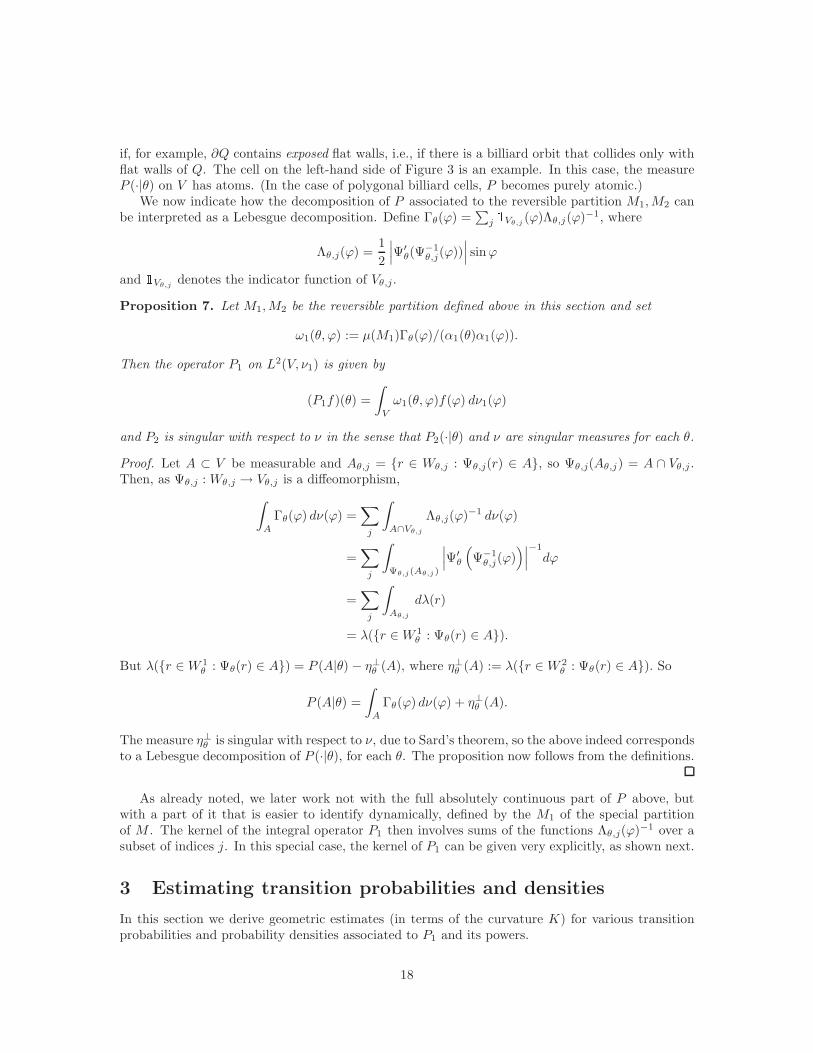
if, for example, ∂Q contains exposed flat walls, i.e., if there is a billiard orbit that collides only withflat walls of Q. The cell on the left-hand side of Figure 3 is an example. In this case, the measureP (·|θ) on V has atoms. (In the case of polygonal billiard cells, P becomes purely atomic.)

We now indicate how the decomposition of P associated to the reversible partition M1,M2 canbe interpreted as a Lebesgue decomposition. Define Γθ(ϕ) =

∑j 1Vθ,j

(ϕ)Λθ,j(ϕ)−1, where

Λθ,j(ϕ) =1

2

∣∣∣Ψ′θ(Ψ

−1θ,j(ϕ))

∣∣∣ sinϕ

and 1Vθ,jdenotes the indicator function of Vθ,j.

Proposition 7. Let M1,M2 be the reversible partition defined above in this section and set

ω1(θ, ϕ) := µ(M1)Γθ(ϕ)/(α1(θ)α1(ϕ)).

Then the operator P1 on L2(V, ν1) is given by

(P1f)(θ) =

∫

V

ω1(θ, ϕ)f(ϕ) dν1(ϕ)

and P2 is singular with respect to ν in the sense that P2(·|θ) and ν are singular measures for each θ.

Proof. Let A ⊂ V be measurable and Aθ,j = r ∈ Wθ,j : Ψθ,j(r) ∈ A, so Ψθ,j(Aθ,j) = A ∩ Vθ,j .Then, as Ψθ,j : Wθ,j → Vθ,j is a diffeomorphism,

∫

A

Γθ(ϕ) dν(ϕ) =∑

j

∫

A∩Vθ,j

Λθ,j(ϕ)−1 dν(ϕ)

=∑

j

∫

Ψθ,j(Aθ,j)

∣∣∣Ψ′θ

(Ψ−1θ,j(ϕ)

)∣∣∣−1

dϕ

=∑

j

∫

Aθ,j

dλ(r)

= λ(r ∈W 1θ : Ψθ(r) ∈ A).

But λ(r ∈W 1θ : Ψθ(r) ∈ A) = P (A|θ) − η⊥θ (A), where η⊥θ (A) := λ(r ∈W 2

θ : Ψθ(r) ∈ A). So

P (A|θ) =

∫

A

Γθ(ϕ) dν(ϕ) + η⊥θ (A).

The measure η⊥θ is singular with respect to ν, due to Sard’s theorem, so the above indeed correspondsto a Lebesgue decomposition of P (·|θ), for each θ. The proposition now follows from the definitions.

As already noted, we later work not with the full absolutely continuous part of P above, butwith a part of it that is easier to identify dynamically, defined by the M1 of the special partitionof M . The kernel of the integral operator P1 then involves sums of the functions Λθ,j(ϕ)−1 over asubset of indices j. In this special case, the kernel of P1 can be given very explicitly, as shown next.

3 Estimating transition probabilities and densities

In this section we derive geometric estimates (in terms of the curvature K) for various transitionprobabilities and probability densities associated to P1 and its powers.

18

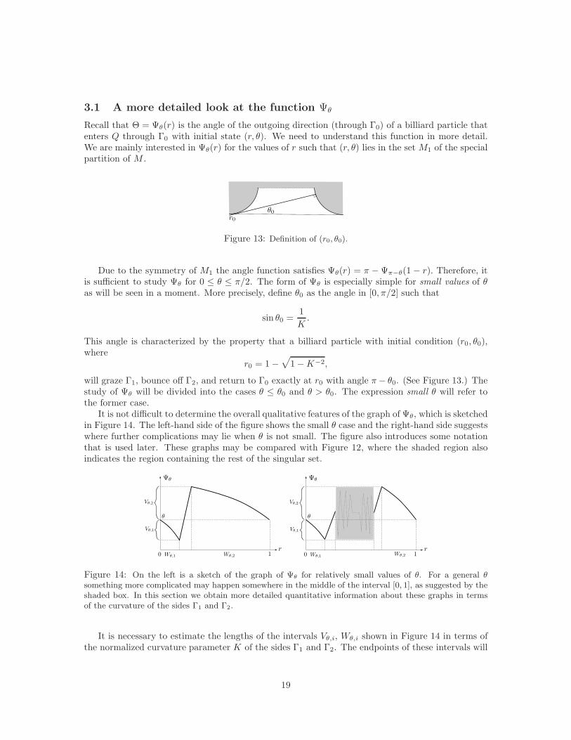
3.1 A more detailed look at the function Ψθ

Recall that Θ = Ψθ(r) is the angle of the outgoing direction (through Γ0) of a billiard particle thatenters Q through Γ0 with initial state (r, θ). We need to understand this function in more detail.We are mainly interested in Ψθ(r) for the values of r such that (r, θ) lies in the set M1 of the specialpartition of M .

Figure 13: Definition of (r0, θ0).

Due to the symmetry of M1 the angle function satisfies Ψθ(r) = π − Ψπ−θ(1 − r). Therefore, itis sufficient to study Ψθ for 0 ≤ θ ≤ π/2. The form of Ψθ is especially simple for small values of θas will be seen in a moment. More precisely, define θ0 as the angle in [0, π/2] such that

sin θ0 =1

K.

This angle is characterized by the property that a billiard particle with initial condition (r0, θ0),where

r0 = 1 −√

1 −K−2,

will graze Γ1, bounce off Γ2, and return to Γ0 exactly at r0 with angle π− θ0. (See Figure 13.) Thestudy of Ψθ will be divided into the cases θ ≤ θ0 and θ > θ0. The expression small θ will refer tothe former case.

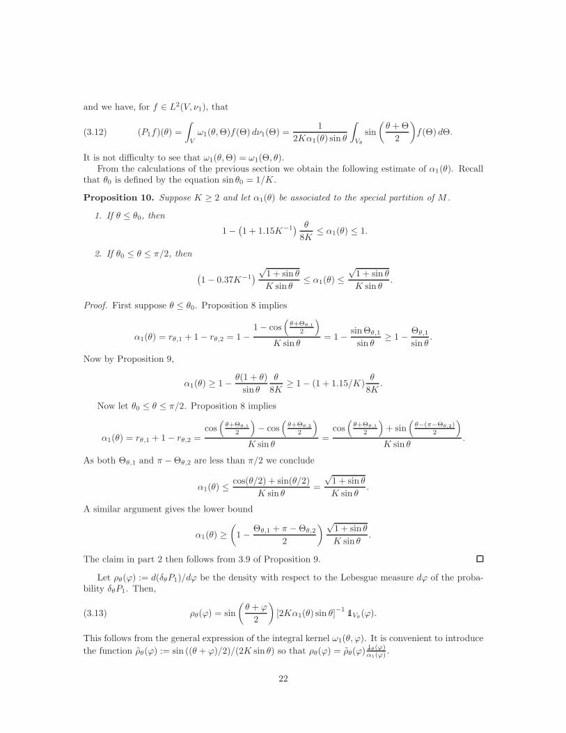
It is not difficult to determine the overall qualitative features of the graph of Ψθ, which is sketchedin Figure 14. The left-hand side of the figure shows the small θ case and the right-hand side suggestswhere further complications may lie when θ is not small. The figure also introduces some notationthat is used later. These graphs may be compared with Figure 12, where the shaded region alsoindicates the region containing the rest of the singular set.

Figure 14: On the left is a sketch of the graph of Ψθ for relatively small values of θ. For a general θsomething more complicated may happen somewhere in the middle of the interval [0, 1], as suggested by theshaded box. In this section we obtain more detailed quantitative information about these graphs in termsof the curvature of the sides Γ1 and Γ2.

It is necessary to estimate the lengths of the intervals Vθ,i, Wθ,i shown in Figure 14 in terms ofthe normalized curvature parameter K of the sides Γ1 and Γ2. The endpoints of these intervals will

19

be denoted as follows (see also Figure 15):

Wθ,1 = [0, rθ,1], Wθ,2 = [rθ,2, 1], Vθ,1 = [Θθ,1, θ], Vθ,2 = [θ,Θθ,2].

Figure 15: The numbers rθ,i and Θθ,i are endpoints of the intervals Wθ,i and Vθ,i as indicated in the text.They are obtained by regarding the trajectories that have a grazing second or first collision with Γ1 ∪ Γ2.

The needed length estimates will be derived from the following proposition.

Proposition 8. Suppose that Q satisfies Assumption 1. Let (r, θ) ∈M , θ ≤ π/2, be the initial stateof a billiard trajectory that collides with ∂Q at most twice (not counting as collisions the initial andfinal states on Γ0), and all collisions happen on Γ1 ∪Γ2. Suppose that one collision is regular and asecond, if it occurs, is grazing. Set Θ = Ψθ(r) and let (s,Θ) be the state at which the particle returnsto Γ0. Then the following hold:

I First (regular) collision with Γ1 and possibly a second (grazing) collision with Γ2. In this case,

(3.1) Kr sin θ = cos

(θ + Θ

2

)− cos θ.

If a second collision does occur and is grazing (see the graph on the left of Figure 15), then

(3.2) K sin Θ = 1 − cos

(θ + Θ

2

).

II First (regular) collision with Γ2, a possibly second (grazing) collision with Γ1. In this case,

(3.3) K(1 − r) sin θ = cos θ − cos

(θ + Θ

2

).

If a second collision does occur and is grazing (see the graph on the middle of Figure 15), then

(3.4) K sin(Θ) = 1 + cos

(θ + Θ

2

).

III If the first collision (with Γ1) is grazing and the second (with Γ2) is regular (see the graph onthe right of Figure 15; this may happen for θ ≤ θ0), then

(3.5) Kr sin θ = 1 − cos θ and cos

(θ + Θ

2

)= 1 −K sin θ.

Proof. This is proved by elementary geometry and trigonometry. We omit the details.

Corollary 1. Under the assumptions of Proposition 8,

(3.6) Ψ′θ(r) = − 2K sin θ

sin(θ+Θ

2

) .

20

Proof. This follows from implicit partial differentiation with respect to r of Equations 3.1 and 3.3of Proposition 8.

We now refine our description of Ψθ with further estimates of Θθ,i in terms of K and θ. Keepin mind throughout that we are here concerned with large K. Unless otherwise stated, we assumethat K is at least 2. We also typically assume in these estimates that θ ≤ π/2 and deal with othervalues by symmetry when needed.

For θ ≤ θ0 defined the map σ(θ) := θ2/8K. The inverse of σ is σ−1(θ) =√

8Kθ, which makessense if θ is sufficiently small, say, less than 1/8K3. The next proposition states that, for θ small,the range of values of Ψθ closely corresponds to the interval [σ(θ), σ−1(θ)].

Proposition 9. Suppose that K ≥ 2. If θ ≤ θ0, then

(3.7)

(1 − θ2

48

)σ(θ) ≤ Θθ,1 ≤ (1 + θ)σ(θ).

If θ ≤ σ(θ0), then

(3.8)

(1 − θ2

12

)σ−1(θ) − θ ≤ Θθ,2 ≤

(1 +

Kθ

9

)σ−1(θ) − θ.

Let now θ0 < θ ≤ π/2. Then

(3.9) Θθ,1 + π − Θθ,2 ≤ 0.73K−1.

Proof. From Proposition 8 we obtain (recall that Θθ,1 < θ)

KΘθ,1 ≥ K sinΘθ,1 = 1 − cos

(θ + Θθ,1

2

)≥ 1 − cos(θ/2)

so that

Θθ,1 ≥ 1 − cos(θ/2)

K=

8(1 − cos(θ/2))

θ2σ(θ) ≥

(1 − θ2

48

)σ(θ).

A similar kind of approximation gives the upper bound for Θθ,1 and the upper and lower bounds forΘθ,2, where the numerical coefficients depend on the assumption K ≥ 2. Note that for the boundsfor Θθ,2 one starts from the identity Θθ,2 = 2 arccos(1 −K sin θ) − θ.

Now suppose that θ0 ≤ θ ≤ π/2 and let Θ stand for either Θθ,1 or π − Θθ,2. Observe thatΘ ≤ Θ := Θπ/2,1. Then, by Proposition 8,

(3.10) Θ ≤ Θ

K sinΘ

[1 − cos

(π

4+

Θ

2

)]

Iterating the inequality Θ ≤ arcsin((1−cos(π/4+Θ/2))/K), with the first step, say, Θ ≤ π/2, yieldsfor K ≥ 2 that Θ < 0.18 and Θ/ sinΘ < 1.006. Then 3.9 follows from Θθ,1 + π−Θθ,2 ≤ 2Θ and theinequality 3.10.

3.2 The kernel of P1 for the special partition

Let Vθ = Vθ,1 ∪ Vθ,2. From Proposition 7 and the general discussion surrounding it, and Corollary1, the integral kernel of the operator P1 can be written as follows (here we use the special partitionof M and, accordingly, the α1 of Proposition 10):

(3.11) ω1(θ,Θ) =µ(M1) sin

(θ+Θ

2

)1Vθ(Θ)

Kα1(θ)α1(Θ) sin θ sin Θ

21

and we have, for f ∈ L2(V, ν1), that

(3.12) (P1f)(θ) =

∫

V

ω1(θ,Θ)f(Θ) dν1(Θ) =1

2Kα1(θ) sin θ

∫

Vθ

sin

(θ + Θ

2

)f(Θ) dΘ.

It is not difficulty to see that ω1(θ,Θ) = ω1(Θ, θ).From the calculations of the previous section we obtain the following estimate of α1(θ). Recall

that θ0 is defined by the equation sin θ0 = 1/K.

Proposition 10. Suppose K ≥ 2 and let α1(θ) be associated to the special partition of M .

1. If θ ≤ θ0, then

1 −(1 + 1.15K−1

) θ

8K≤ α1(θ) ≤ 1.

2. If θ0 ≤ θ ≤ π/2, then

(1 − 0.37K−1

) √1 + sin θ

K sin θ≤ α1(θ) ≤

√1 + sin θ

K sin θ.

Proof. First suppose θ ≤ θ0. Proposition 8 implies

α1(θ) = rθ,1 + 1 − rθ,2 = 1 −1 − cos

(θ+Θθ,1

2

)

K sin θ= 1 − sinΘθ,1

sin θ≥ 1 − Θθ,1

sin θ.

Now by Proposition 9,

α1(θ) ≥ 1 − θ(1 + θ)

sin θ

θ

8K≥ 1 − (1 + 1.15/K)

θ

8K.

Now let θ0 ≤ θ ≤ π/2. Proposition 8 implies

α1(θ) = rθ,1 + 1 − rθ,2 =cos(θ+Θθ,1

2

)− cos

(θ+Θθ,2

2

)

K sin θ=

cos(θ+Θθ,1

2

)+ sin

(θ−(π−Θθ,2)

2

)

K sin θ.

As both Θθ,1 and π − Θθ,2 are less than π/2 we conclude

α1(θ) ≤cos(θ/2) + sin(θ/2)

K sin θ=

√1 + sin θ

K sin θ.

A similar argument gives the lower bound

α1(θ) ≥(

1 − Θθ,1 + π − Θθ,2

2

) √1 + sin θ

K sin θ.

The claim in part 2 then follows from 3.9 of Proposition 9.

Let ρθ(ϕ) := d(δθP1)/dϕ be the density with respect to the Lebesgue measure dϕ of the proba-bility δθP1. Then,

(3.13) ρθ(ϕ) = sin

(θ + ϕ

2

)[2Kα1(θ) sin θ]

−1 1Vθ(ϕ).

This follows from the general expression of the integral kernel ω1(θ, ϕ). It is convenient to introduce

the function ρθ(ϕ) := sin ((θ + ϕ)/2)/(2K sin θ) so that ρθ(ϕ) = ρθ(ϕ)1θ(ϕ)α1(ϕ) .

22

Proposition 11. We suppose that K ≥ 2, θ ≤ π/2.

1. Let θ ≤ θ0 and ϕ ∈ Vθ. Then

(4K)−1 ≤ ρθ(ϕ) ≤ ρθ(ϕ) ≤ (1 + 0.21θ/K) ρθ(ϕ).

If in addition ϕ ∈ Vθ,1, then ρθ(ϕ) ≤ (2K)−1 and P1(Vθ,1|θ) ≤ (1 + 0.43K−2)3θ(8K)−1.

2. Now suppose that θ ≥ θ0. Then

ρθ(ϕ) ≥ cϕ :=1

2min

sin

ϕ

2, cos

ϕ

2

.

Proof. These are all straightforwardly derived from Proposition 10. For part 2, observe:

ρθ(ϕ) =ρθ(ϕ)

α1(θ)≥

sin(θ+ϕ

2

)

2(1 + sin θ)1/2=

1

2

sin θ2 cos ϕ2 + cos θ2 sin ϕ

2

sin θ2 + cos θ2

≥ cϕ

3.3 Upper bound for the action of P1 on probability densities

We need further notation before continuing. Recall the map σ(ϕ) = ϕ2/8K. Define

an = σn(1/K) = 8K(8K2

)−2n

for n = 0, 1, . . . and An = [an, π − an]. Recall that sin θ0 = 1/K, so a0 is approximately θ0.We are interested in the action of powers of P1 on probability density functions g with respect to

the Lebesgue measure m on [0, π]. Let mg be the measure on [0, π] having density function g. LetP ∗

1 be the Markov operator on densities so, by definition, P ∗1 g is the density of the measure mgP1.

It follows from the definition of Θθ,i that ϕ ∈ Vθ = [Θθ,1,Θθ,2] if and only if θ ∈ Vϕ. With this inmind one obtains

(P ∗1 g)(θ) =

1

2K

∫

Vθ

sin

(ϕ+ θ

2

)[α1(ϕ) sinϕ]−1 g(ϕ) dϕ.

Proposition 12. Let K ≥ 2, θ ≤ π/2, and g a probability density on [0, π] with respect to m. Ifθ ≤ Θa0,1,

(P ∗1 g)(θ) ≤ 0.93

‖g|Vθ∩Ac0‖∞

Kσ−1(θ)

and if θ > Θa0,1,

(P ∗1 g)(θ) ≤ 1.45

‖g|Vθ∩Ac0‖∞

K+ 0.62

where we set ‖g|Vθ∩Ac0‖∞ = 0 if Vθ ∩Ac0 is empty. In particular,

‖P ∗1 g‖∞ ≤ 1.45

‖g‖∞K

+ 0.62.

The value 0.99a1 can be substituted for Θa0,1 in the above conditions on θ.

23

Proof. We write (P ∗1 g)(θ) = I1 + I2, where

I1 =1

2K

∫

Vθ∩A0

sin(ϕ+θ

2

)

α1(ϕ) sinϕg(ϕ) dϕ, I2 =

1

2K

∫

Vθ∩Ac0

sin(ϕ+θ

2

)

α1(ϕ) sinϕg(ϕ) dϕ.

Using Proposition 10, sin((θ + ϕ)/2)/√

1 + sinϕ ≤ 1, and K ≥ 2, we obtain

I1 ≤ 0.62mg(Vθ ∩A0), I2 ≤ 0.53‖g|Vθ∩Ac0‖∞K−1Iθ,

where Iθ =∫Vθ∩Ac

0sin((ϕ+ θ)/2)/ sinϕdϕ. We now estimate Iθ by writing Iθ = J1 + J2, where J1 is

the integral of the argument of Iθ over Vθ,1 ∩ Ac0 and J2 is the integral of that same function overVθ,2 ∩Ac0. As ϕ+ θ ≤ 2θ on Vθ,1 and ϕ+ θ ≤ 2ϕ on Vθ,2, then

J1 ≤ sin θ

∫

Vθ,1∩Ac0

dϕ

sinϕ, J2 ≤ m(Vθ,2 ∩Ac0).

A straightforward computation, which uses the approximation 0 ≤ −x lnx < 0.74√x, 0 < x < 1,

shows that J1 ≤ c1 sin θ[(θ ∧ a0)/(Θθ,1 ∧ a0)]1/2, where the wedge symbol represents the minimum

of the two numbers and c1 can be taken to be 0.78 if θ ≤ a0 and 0.74 if θ ≤ a1. (These numbersarise from multiplying 0.74 by an upper-bound for ϕ/ sinϕ over ϕ ≤ a0 and ϕ ≤ a1, respectively.)

If θ ≤ a0 one shows that sin θ[(θ ∧ a0)/(Θθ,1 ∧ a0)]1/2 ≤ θ3/2/Θ

1/2θ,1 ≤ c2σ

−1(θ), where c2 can be

taken, based on Proposition 9, to equal 1.003 for θ ≤ a0 and 1.00001 for θ ≤ a1. Thus J1 ≤ cσ−1(θ),where c = c1c2, if θ ≤ a0. Also observe that m(Vθ,2 ∩A0) ≤ Θθ,2 ∧ a0 ≤ 1.004σ−1(θ) ∧ a0, where wehave used Proposition 9 and K ≥ 2. The first inequality of the proposition now follows, in whichthe number 0.93 is seen to come from 0.53(1.004 + 0.74). The cases Θθ,1 ≤ a0 ≤ θ and Θθ,1 ≥ a0

are similarly treated, leading to the general expression

(P ∗1 g)(θ) ≤ 0.62mg(Vθ ∩A0) + sθ

‖g|Vθ∩Ac0‖∞

K

where sθ = 1.45 for θ ≥ a1 and sθ = 0.93σ−1(θ) for θ ≤ a1. The proposition results immediatelyfrom this inequality.

3.4 Lower bounds for transitions to middle intervals

Let P1(A|θ) := (δθP1)(A), representing the probability that the scattered angle lies in A given thatthe angle of incidence is θ and that the event M1 holds. Similarly, define Pn1 (A|θ) := (δθP

n1 )(A) for

all n ≥ 1. The following notation is used: Zϕ := [ϕ, π − ϕ], for some ϕ ∈ [0, π/2], and Z0 := Zθ0 .Zcϕ denotes the complement in [0, π].

Lemma 2. We assume that K ≥ 2, θ, ϕ both lie in [0, π/2], and that ϕ ≤ θ0.

1. If θ ∈ Z0, then

P1(Zcϕ|θ) ≤

(1 + 0.38K−1

) ϕ (1 + ϕ)1/2

2≤ 0.75ϕ.

2. If θ ∈ Zc0, then

P1(Zcϕ|θ) ≤

(1 + 0.43K−2

) ϕ(1 + ϕ

θ

)

4K.

24

Proof. Keeping in mind the expression 3.13, note that

P1(Zcϕ|θ) =

∫ ϕ

0

[ρθ(ψ) + ρθ(π − ψ)] dψ ≤ 1

2Kα1(θ) sin θ

∫ ϕ

0

[sin

(θ + ψ

2

)+ cos

(θ − ψ

2

)]dψ.

It follows from the identity

sin

(θ + ψ

2

)+ cos

(θ − ψ

2

)= (1 + sin θ)1/2 (1 + sinψ)1/2

and Proposition 10 that

P1(Zcϕ|θ) ≤

ϕ (1 + sinϕ)1/2

(1 + sin θ)1/2

2Kα1(θ) sin θ≤ (1 + 0.38/K)

ϕ(1 + sinϕ)1/2

2

as claimed. For part 2, observe that Θϕ,2 ≤ Θθ0,2 = π − θ0 ≤ π − ϕ. Therefore,

P1(Zcϕ|θ) =

∫ ϕ

0

ρθ(ψ) dψ ≤ϕ sin

(θ+φ

2

)

2K sin θα1(θ).

Using the estimates of α1(θ) from Proposition 10 (recall that α1(θ) := λ(M1(θ))) and assumingK ≥ 2, which is used when simplifying expressions such as θ/ sin θ and taking the reciprocal ofα1(θ)), we can obtain 2.

Let Θ0,Θ1, . . . be the Markov chain for P1 with initial state Θ0 = θ. The next propositionquantifies the tendency of the Markov chain to move points in (0, π) towards the middle range ofangles.

Proposition 13. We suppose that K ≥ 2. Let ϕ ≤ θ0 and θ ∈ Zσ(ϕ) be fixed. Then

Pn+21 (Zcϕ|θ) ≤

1.77 + 0.10nϕ2

K.

for all n ≥ 1.

Proof. We prove the proposition by induction. Let Θ0,Θ1, . . . be the Markov chain for P1 withinitial state Θ0 = θ ∈ Zσ(ϕ). For the induction step we need to estimate

Iθ := P1(Θ2 ∈ Zcϕ|Θ0 = θ) =

∫ π

0

ρθ(θ′)P1(Z

cϕ|θ′) dθ′.

Assume first that σ(ϕ) ≤ θ ≤ ϕ and write Iθ = I1 + I2 + I3, where

I1 =

∫ ϕ2/2

0

ρθ(θ′)P1(Z

cϕ|θ′) dθ′, I2 =

∫ ϕ

ϕ2/2

ρθ(θ′)P1(Z

cϕ|θ′) dθ′, I3 =

∫ π

ϕ

ρθ(θ′)P1(Z

cϕ|θ′) dθ′.

Transition probabilities involved in these and other integrals below can be derived from Lemma 2.The following, in particular, will be needed:

(TP1) If θ ∈ Zϕ, then P1(Zcϕ|θ) ≤ 0.75ϕ and P1(Z

cϕ2/2|θ) ≤ 0.38ϕ2

(TP2) If θ ∈ Zϕ2/2 \ Zϕ, then P1(Zcϕ|θ) ≤ 0.70K−1

(TP3) If θ ∈ Zσ(ϕ) \ Zϕ, then P1(Zcϕ2/2|θ) ≤ 0.63ϕ2

25

(TP4) If θ ∈ Zσ(ϕ), then P1(Zcσ(θ)|θ) ≤ 0.10ϕ2/K.

Then using TP3 above,

I1 ≤∫ ϕ/2

0

ρθ(θ′) dϕ ≤ P1([0, ϕ

2/2]|θ) ≤ P1(Zcϕ2/2|θ) ≤ 0.63ϕ2.

Using TP2 we have I2 ≤ (0.70/K)P1([ϕ2/2, ϕ]|θ) ≤ 0.70/K. Note that I3 only needs to be integrated

over Zϕ since Θθ,2 ≤ π − ϕ. Using TP1, we have I3 ≤ 0.75ϕP1(Zϕ|θ) ≤ 0.75ϕ. Approximating θ0by 1/K, we obtain the sum Iθ ≤ 1.77

K . Now let θ ∈ Zϕ and write Iθ = I1 + I2, where

I1 =

∫

Zϕ2/2

ρθ(θ′)P1(Z

cϕ|θ′) dθ′ ≤

0.75

KP1(Zϕ2/2|θ) ≤

0.75

K

where we have used TP1 and TP2, and

I2 =

∫

Zcϕ2/2

ρθ(θ′)P1(Z

cϕ|θ′) dθ′ ≤

∫

Zcϕ2/2

ρθ(θ′) dθ′ = P1(Z

cϕ2/2|θ) ≤ 0.38ϕ2

where we have used TP1. Thus Iθ ≤ 0.94K . Therefore, if θ ∈ Zσ(ϕ), ϕ ≤ θ0, and K ≥ 2, then

P1(Θ2 ∈ Zcϕ|Θ0 = θ) ≤ 1.77

K.

Now set C2 = 1.77 and, for each positive integer k suppose that P k+21 (Zcϕ|θ) is bounded above by

Ck+2/K, for ϕ ≤ θ0, θ ∈ Zσ(ϕ), and k = 0, 1, . . . , n. Then P k+31 (Zcϕ|θ) can be estimated as follows:

∫ π

0

ρθ(θ′)P k+2

1 (Zcϕ|θ′) dθ′ =

∫

Zσ(ϕ)

ρθ(θ′)P k+2

1 (Zcϕ|θ′) dθ′ +

∫

Zcσ(ϕ)

ρθ(θ′)P k+2

1 (Zcϕ|θ′) dθ′

≤ Ck+2

K

∫

Zσ(ϕ)

ρθ(θ′) dθ′ +

∫

Zcσ(ϕ)

ρθ(θ′) dθ′

=Ck+2

KP1(Zσ(ϕ)|θ) + P1(Z

cσ(ϕ)|θ) ≤

Ck+2 + 0.10ϕ2

K

where at the last step we have used TP4. Therefore, Ck+3 ≤ Ck+2+0.10ϕ2, concluding the proof.

In the proof of the next corollary and later in the paper we use ρ(n)θ to denote the density of the

probability measure δθPn1 relative to the Lebesgue measure on [0, π].

Corollary 2. Let cθ be as defined in Proposition 11 and Cn+2 = 1.77 + nθ20 the constant thatappears in Proposition 13 (setting ϕ = θ0). Let η be a probability measure on (0, π) whose supportis contained in Zσ(θ0). Then for all n ≥ 3 the density function of ηPn1 , relative to the Lebesguemeasure, satisfies

d(ηPn1 )

dθ≥ cθ

(1 − Cn−1

K

).

for all θ ∈ Zθ0 .

Proof. Observe that

ηPn1 =

∫δθ′P

n1 dη(θ

′),

26

so it suffices to prove the lemma for measures of the form η = δθ′ . In this case, if θ′ ∈ Zσ(θ0), then

ρ(n)θ′ (θ) ≥

∫

Z0

ρ(n−1)θ′ (ψ)ρψ(θ) dψ ≥ cθP

n−11 (Z0|θ′).

The desired conclusion now follows from Proposition 13.

We have already introduced the numbers an = σn(1/K) = 8K(1/8K2)2n

and the intervalsAn = [an, π − an]. Define in addition bn = an/(2K)n+2, for n = 0, 1, . . . and Bn = [bn, π − bn].Then bn > an+1 > bn+1, so that

Bn ⊂ An+1 ⊂ Bn+1.

Lemma 3. We define δn := 3/(2K)n. Let n ≥ m ≥ 1 and θ ∈ Bn. Then

Pm1 (Bn−m|θ) ≥m−1∏

i=0

(1 − δn−i).

Proof. The proof is by induction in m. The case m = 1 amounts to the following consequence ofProposition 2: for θ ∈ Bn and K ≥ 2

P1(Bcn−1|θ) ≤

(1 +

0.43

K2

) bn−1

(1 + bn−1

bn

)

4K≤ δn.

So suppose that the claim holds for m − 1, that is, Pm−11 (Bn−m+1|θ) ≥ (1 − δn−m+2) . . . (1 − δn).

Then, making use of Proposition 2 again and the induction hypothesis, we obtain

Pm1 (Bn−m|θ) ≥∫

Bn−m+1

ρ(m−1)θ (ϕ)P1(Bn−m|ϕ) dϕ

≥ (1 − δn−m+1)

∫

Bn−m+1

ρ(m−1)θ (ϕ) dϕ

= (1 − δn−m+1)Pm−11 (Bn−m+1|θ)

≥m−1∏

i=0

(1 − δn−i),

as claimed.

Proposition 14. Assume that K ≥ 2. Let θ ∈ An, n ≥ 0, and suppose that m ≥ n+ 2. Then

Pm1 (A0|θ) ≥(

1 − 2.06 + 0.10(m− n− 2)θ20K

) n∏

i=2

(1 − δi).

Proof. It can be derived from Proposition 2 that P1(Ac1|b1) ≤ 0.29/K. If ϕ ∈ B1 and m ≥ n + 2,

it then follows from Proposition 13 and this inequality (in the third and last inequalities below,

27

respectively),

Pm−n+11 (A0|ϕ) ≥ Pm−n+1

1 (A0|b1)

≥∫

A1

ρb1(ψ)Pm−n1 (A0|ψ) dψ

≥(

1 − 1.77 + 0.10(m− n− 2)θ20K

)∫

A1

ρb1(ψ) dψ

=

(1 − 1.77 + 0.10(m− n− 2)θ20

K

)P1(A1|b1)

≥ 1 − 2.06 + 0.10(m− n− 2)θ20K

.

Consequently,

Pm1 (A0|θ) ≥∫

B1

ρ(n−1)θ (ϕ)Pm−n+1

1 (A0|ϕ) dϕ

≥(

1 − 2.06 + 0.10(m− n− 2)θ20K

)Pn−1

1 (B1|θ).

But by Lemma 3, Pn−11 (B1|θ) ≥ (1 − δ2) . . . (1 − δn), proving the claim.

Corollary 3. Assume K ≥ 2. If θ ∈ An, ϕ ∈ A0, and m ≥ n+ 2, then

ρ(m+1)θ (ϕ) ≥ cϕ

(1 − 2.06 + 3(K − 1)−1 + 0.10(m− n− 2)K−2

K

).

Proof. If ϕ ∈ A0 and ψ ∈ A0, then by Proposition 11 (2) ρψ(ϕ) ≥ cϕ, where cϕ was defined in thatproposition. Now let θ ∈ An, ϕ ∈ A0, and m ≥ n+ 2. Then

ρ(m+1)θ (ϕ) ≥

∫

A0

ρ(m)θ (ψ)ρψ(ϕ) dψ ≥ cϕ

∫

A0

ρ(m)θ (ϕ) dϕ = cϕP

m1 (A0|θ)

≥ cϕ

(1 − 2.06 + 0.10(m− n− 2)θ20

K

) n∏

i=2

(1 − δi).

In the last step above we have used Proposition 14. The product on the right-hand side of the aboveinequality can be estimated by

∏ni=2(1 − δi) ≥ 1 − 3/K(K − 1) for all n. Replacing 1/K for θ0 we

obtain the claim.

We summarize the main point of the above observations in the following lemma.

Lemma 4. Let n ≥ 0 and m ≥ n+ 2. Let η be any probability measure on (0, π). Then there existsa positive constant Cm−n depending on m− n but independent of η, such that, for θ ∈ A0,

d(ηPm1 )

dθ≥ cθ

(1 − Cm−n

K

)η(An).

If K ≥ 2, we can choose Cl = 5.01 + 0.03l.

Proof. This is due to the above corollary and that (d(ηPm1 )/dθ)(θ) ≥∫An

ρ(m)ϕ (θ) dη(ϕ).

28

4 Mixing speed of the billiard Markov processes

Recall from Lemma 12 that ‖P ∗1 g‖∞ ≤ 1.45(‖g‖∞/K) + 0.62, where P ∗

1 g is the density of mgP1

with respect to Lebesgue measure m on [0, π]. Thus, if K ≥ 2 and ‖g‖∞ ≤ 2.3, then ‖P ∗1 g‖∞ ≤ 2.3.

Set γ = 1.45/K and δ = 0.62/(1 − γ). Observe that the map F (x) = γ(x − δ) + δ is a contractionwith fixed point δ, and Fn(x) − δ = γn(x − δ). (As always, we assume K ≥ 2.) Thus for all α > 0there exists an n0 such that ‖P ∗

1ng‖∞ ≤ α(‖g‖∞ − δ) + δ for all n ≥ n0. In particular, for n0 big

enough, we can assume that ‖P ∗1ng‖∞ ≤ 2.3, for all n ≥ n0.

From Lemma 4,

(P ∗1

3g)(θ) ≥ cθ

(1 − C2

K

)(mgP1)(A0)

and, assuming ‖g‖∞ ≤ 2.3, then mgP1(Ac0) ≤ 4.6/K, from which we obtain

(P ∗1

3g)(θ) ≥ cθ

(1 − C

K

),

where C = C2 + 4.6 < 9.7. Define

p := (2 −√

2)(1 − C/K), h(θ) := cθ

(1 − C

K

)1A0(θ).

Notice that mh(A0) = (2 cosa0−√

2)(1−C/K)), so by making C slightly bigger, and K sufficientlylarge, the higher order terms of cosa0 = 1+O(K−2) can be absorbed into C and we have p = mh(A0).

Definition 2. A probability density g will be called proper if g|A0 ≥ h and ‖g‖∞ ≤ 2.3.

Lemma 5. If g is a proper probability density then the probability density g1 defined by

mg1 :=mg −mh

1 − pP 3

1

is also proper, assuming that K is big enough (say, K > 10).

Proof. This is an immediate consequence of the above observations. Note that (mg −mh)/(1− p) isindeed a probability measure since mg([0, π])−mh([0, π]) = 1−p, and it has density (g−h)/(1−p),which is positive as g is proper.

We can then iterate the operation g 7→ g1 defined in Lemma 5 to obtain the following for anyproper density g. Let gn be the resulting density after n iterations. Then gn is also proper and

(4.1) mgP3n1 = (1 − p)nmgn +

n−1∑

j=0

(1 − p)jmhP3(n−j)1 .

Proposition 15. Suppose K is big enough (say, K > 10) and let η = mg for any probability densityg on [0, π]. Then there exists a positive integer r such that

‖ηP r+3n1 − ν1‖TV ≤ 2(1 − p)n

for all positive integers n, where ‖·‖TV is the total variation norm and ν1 is the invariant probabilityassociated to P1. (See Section 2.5.)

Proof. After applying P r1 to mg for r big enough we obtain a probability measure whose density isproper. The invariant measure ν1 is itself proper. Then using the expansion 4.1 for both ηP r1 andν1 we obtain ηP r+3n

1 − ν1 = (1− p)n(η′ − ν′), where η′ and ν′ are probability measures. Now recallthat ‖η′ − ν′‖TV ≤ 2.

29

If f, g are essentially bounded functions and g ≥ 0 such that mg([0, π]) = 1, it follows fromProposition 15 that there exists a constant C = C(g) such that

(4.2) |(mgPn1 )(f) − ν1(f)| ≤ C‖f‖∞(1 − p)n/3

for all positive n.

Corollary 4. Assume that K is sufficiently big (say, K > 10). Let f ∈ L∞([0, π], ν1)∩L2([0, π], ν1),where ν1 is the P1-stationary probability measure, and suppose that ν1(f) = 0. Then there exists aconstant Cf > 0 such that

|〈Pn1 f, f〉ν1 | ≤ Cf (1 − p)n/3

for every integer n.

Proof. Recall that (dν1/dm)(θ) = α1(θ) sin θ/µ1(M1), where the notations are defined in Section2.1 and m is the Lebesgue measure. We decompose f = f+ − f− into its positive and negative partsand define g±(θ) := f±(θ)(dν1/dm)(θ), which are essentially bounded functions with respect to m.Then

|〈Pn1 f, f〉ν1 | ≤ |(mg+Pn1 )(f)| + |(mg−P

n1 )(f)|.

If we now set Cf = C(g+) + C(g−), then the claim follows from 4.2.

5 Compactness and spectral gap

We show here that P1 is a Hilbert-Schmidt operator, hence compact, and P is in general quasi-compact, and provide an estimate of the spectral gap.

Proposition 16. The operator P1 on L2([0, π], ν1) is Hilbert-Schmidt .

Proof. Set V = [0, π] and recall that (P1f)(θ) =∫Vω1(θ, ϕ)f(ϕ) dν1(ϕ) for f ∈ L2(V, ν1), where

ω1(θ, ϕ) =µ1(M1) sin

(θ+ϕ

2

)1Vθ(ϕ)

Kα1(θ)α1(ϕ) sin θ sinϕ

and Vθ = Vθ,1 ∪ Vθ,2. (See the beginning of Section 3 for the notations.) We need to verify that theintegral kernel ω1 is a square integrable function on V × V with the product measure ν1 × ν1. Dueto the symmetry ω1(θ, ϕ) = ω1(π − θ, π − ϕ), the L2-norm of ω1 is

2

∫ π/2

0

∫

V

ω21(θ, ϕ) dν1(ϕ) dν1(θ) =

1

2K2

∫ π/2

0

∫

Vθ

sin2(θ+ϕ

2

)

α1(θ)α1(ϕ) sin θ sinϕdϕdθ

is finite. (We have used here the expression for ν1 given at the beginning of Subsection 2.1.) Observethat if θ0 ≤ θ ≤ π/2 then both θ and ϕ ∈ Vθ are at a bounded distance away from 0 and π. Thequantities α1(θ) and ϕ1(ϕ) are also bounded away from 0 for all angles. (In fact, they approach 1for angles close to 0 or π.) So it suffices to check that I := I1 + I2 is finite, where Ii is defined by

Ii :=

∫ θ0

0

∫

Vθ,i

sin2(θ+ϕ

2

)

sin θ sinϕdϕdθ.

Note that sin(θ+ϕ

2

)≤ sin θ on Vθ,1 = [Θθ,1, θ], and sin

(θ+ϕ

2

)≤ sinϕ on Vθ,2 = [θ,Θθ,2]. So

I1 ≤∫ θ0

0

∫ θ

Θθ,1

(sin θ/ sinϕ) dϕdθ ≤ C

∫ θ0

0

sin θ ln(θ/Θθ,1) dθ.

30

Keeping in mind the bounds on Θθ,i obtained in Proposition 9, we have Θθ,1 ≥ cθ2, for some positiveconstant c, from which it follows that the integral is finite. Now

I2 ≤∫ θ0

0

∫ θ

Θθ,1

(sinϕ/ sin θ) dϕdθ ≤∫ θ0

0

1

sin θ

[Θ2θ,2 − θ2

2

]dθ

and we know that Θθ,2 is bounded above by a constant times√θ. Thus I2 is also finite.

We now turn to the estimate of the spectral gap for P1.

Lemma 6. Let T be a bounded self-adjoint operator of norm 1 in the Hilbert space H := L2(V, µ),where µ is a probability measure on the Lebesgue space V . Let H0 be the orthogonal complementof the constant functions and define the spectral gap γ(T ) = 1 − ρ0(T ), where ρ0(T ) is the spectralradius of T |H0 . Also suppose that 〈T nf, f〉 ≤ Cfλ

n for a positive λ < 1 and all f ∈ H0 ∩ L∞(V, µ)and positive integer n. Then

1. ‖T nf‖2 ≤ ‖f‖2λn for all f ∈ H0 and positive integer n;

2. γ(T ) ≥ 1 − λ.

Proof. We may assume that ‖f‖2 = 1. Since L∞(V, µ) is dense in H , we may also assume that thefunctions are essentially bounded. Let T =

∫σλ dE(λ) be the spectral decomposition of T , where

σ ⊂ R denotes the spectrum of T and E is the corresponding projection-valued measure. Writedµf (λ) := 〈dE(λ)f, f〉. Then for p ≥ 1

‖T nf‖22 =

∫

σ

λ2ndµf (λ) =

([∫

σ

(λ2n/p)p dµf (λ)

]1/p)p

≥(∫

σ

λ2n/p dµf (λ)

)p= ‖T n/pf‖2p

2 .

We have used that ‖g‖1 ≤ ‖g‖p for probability measures. Now let p = n/m, where n ≥ m. Then

‖Tmf‖2 ≤ ‖T nf‖m/n2 = 〈T 2nf, f〉m/2n ≤ Cm/2nf λm.

By letting n go to ∞ we conclude (1).

Now recall that ρ0(T ) = limm→∞ ‖(T |H0)n‖1/n

2 . For any ǫn such that lim ǫn = 0 we can choosefn ∈ H0 of norm 1 for which

‖(T |H0)n‖1/n

2 ≤ ‖T nfn‖1/n2 + ǫn ≤ λ+ ǫn,

where we have used part (1). By passing to the limit we obtain (2).

Thus we obtain for the spectral gap of P1 the estimate γ ≥ 1 − (1 − p)1/3 where, we recall,p = (2 −

√2)(1 − C/K) whenever K is sufficiently big. Thus for large values of K we get

γ ≥ 0.25 − 0.35C/K.

Proposition 17. For the same C > 0 as above (see paragraph just prior to Definition 2) and some

N ≥ 3, the spectral gap of P1 satisfies γ ≥ 1− (C/K)1/N for all K > 0. In particular, the gap mustapproach the maximum possible value 1 for very large values of K.

Proof. We know from Proposition 15 that for any probability measure η absolutely continuouswith respect to the Lebesgue measure ηPn1 converges to ν1 exponentially fast in the total variationnorm. In fact, any measure η that does not have atoms at 0 and π satisfies this property sinceone application of P1 makes the measure absolutely continuous. With this in mind, we can now

31

go back to the argument at the beginning of Section 4 and improve on the estimate used in thespecification of p. More precisely, it is now possible to find a positive integer N such that, for anygiven probability density g on V with respect to the Lebesgue measure m

P ∗1Ng ≥

(1 − C

K

)dν1dm

.

That is, we have replaced the function cθ with the density of ν1. Accordingly, we redefine h(θ) andp, so that p = 1 − C/K. (This has been achieved at the cost of increasing the number of iterationsof P1 needed for each step in the coupling argument.) The spectral gap γ can now be estimated,just as done above (using Corollary 4 and Lemma 6), by

γ ≥ 1 − (1 − p)1/N = 1 − (C/K)1/N

as claimed.

With this remark, all the claims involved in Theorem 2 have been proved. Theorem 1 followsfrom Theorem 2 and the next general observation. (See Theorem 9.9 in [20].)

Proposition 18. Let K and T be bounded self-adjoint operators on a Hilbert space and supposethat K is compact. Then the essential spectrum of T +K is contained in the essential spectrum ofT . In particular, if ‖T +K‖2 = 1 and ‖T ‖2 < 1, then the spectral gap of T +K satisfies

γ(T +K) ≥ min1 − ‖T ‖2, γ(K).

The theorem follows from letting K = α1P1 and T = α2P2. Observe that, due to Proposition 10we have 1 − ‖T ‖2 ≥ inf α1 ≥ (1 − 0.37/K)

√2/K.

6 Glossary of symbols

We summarize below the notation used across more than one section of the text. Symbols not listedhere are likely to be used only locally, and their first occurrence should be near the places wherethey are employed.

1. Measures

• λ Lebesgue measure on the unit interval I = [0, 1]; occasionally denoted ds, dx, etc.

• m (non-normalized) Lebesgue measure on V = [0, π]; often denoted dθ, dφ, etc.

• mg finite measure on V with density g ∈ L1(V,m); i.e., dmg/dm = g

• ν = mg, where g(θ) = 12 sin θ

• νg finite measure on V with density g ∈ L1(V, ν); i.e., dνg/dν = g

• µ = λ⊗ ν probability measure on M = I × V invariant under the return billiard map T

• νj conditional measures associated to a measurable partition Mj of M (Subsection 2.5)

• δθ Dirac delta measure on V concentrated at θ

• η symbol often used for general purpose measure

2. Sets

• Q ⊂ R2 the (micro) billiard cell

• Γi parts of the boundary of Q (Subsections 1.1 and 2.1)

32

• I = [0, 1], V = [0, π], M = I × V

• M phase space of the billiard system on Q (Subsection 2.1)

• Mi parts of M associated to the Γi (Subsection 2.1)

• Sm singular sets associated to the billiard map F on M (Subsection 2.1)

• Wθ = I × θ, W iθ , Wθ,j, Vθ,j (Subsection 2.6 for a general partition)

• Wθ,j , Vθ,j , Vθ = [Θθ,1,Θθ,2] (Subsection 3.1 for the special partition)

• Zϕ = [ϕ, π − ϕ], Z0 = Zθ0

• An = Zan , where an = σn(1/K), Bn = Zbn , where bn = an/(2K)n+2 (Subsection 3.3)

• Mi elements of a measurable partition of M (Subsection 2.5). Different partitions areemployed at different places in the text, and are defined where they arise; for the maintheorems and throughout most of Section 3 we use the special partition, which is definedjust prior to the statement of Theorem 2.

3. Functions, maps, and operators

• F billiard map on M

• T return billiard map on M

• Ψr(θ) = Θ(r, θ) angle component of T (r, θ)

• P Markov (reflection) operator of random billiard (Definition 1)

• Pi conditional operator associated to a partition Mi of M (Subsection 2.5)

• αi probability function associated to a partition Mi of M (Subsection 2.5)

• π2 : M → V the natural component projection

• J used for the map (r, θ) → (1 − r, π − θ) on M

• J used for the maps (r, θ) → (r, π − θ) on M , θ → π − θ on V , and the induced unitaryoperator on L2(V, ν)

• Ii : L2(V, ν) → L2(V, νi), inclusion operator

• Mi : L2(V, νi) → L2(V, ν), multiplication by αi

• ω1(θ, ϕ), integral kernel of P1 (Subsection 2.6 general; Subsection 3.2 for the specialpartition)

• Θ1,Θ2, . . . Markov chain for the angle process with Markov operator P

4. Miscellaneous

• γ, γ(K) spectral gap of an operator K; γ1 = γ(P1)

• K scale-invariant curvature of Γi (defined just prior to Theorem 1)

• θ0 is defined by sin θ0 = 1/K

• rθ,i, Θθ,i (Subection 3.1)

• 1A the indicator function of A

Acknowledgment. Hong-Kun Zhang is partially supported by NSF DMS-0901448.

Email addresses: feres@math.wustl.edu, hongkun@math.umass.edu

33

References

[1] L.A, Bunimovich, On the ergodic properties of nowhere dispersing billiards, Comm. Math.Phys. 65 (1979), 295–312.

[2] L.A, Bunimovich, Mushrooms and other billiards with divided phase space, Chaos 11 (2001),802808.

[3] L.A, Bunimovich, Ya.G. Sinai, & N.I. Chernov, Markov partitions for two-dimensionalhyperbolic billiards, Russian Math. Surveys 45 (1990) 105–152.

[4] L.A, Bunimovich, Ya.G. Sinai, & N.I. Chernov, Statistical properties of two-dimensionalhyperbolic billiards, Russian Math. Surveys 46 (1991) 47–106.

[5] C. Cercignani and D.H. Sattinger, Scaling Limits and Models in Physical Process,Birkhauser, DMV Seminar, Band 28, 1998.

[6] N.I. Chernov, Decay of correlations in dispersing billiards, J. Stat. Phys. 94 (1999), 513–556.

[7] N.I. Chernov and R. Markarian, Chaotic Billiards, Mathematical Surveys and Monographs,127, AMS, Providence, RI, 2006.

[8] N.I. Chernov and L. S. Young, Decay of correlations for Lorentz gases and hard balls.Hard ball systems and the Lorentz gas. Encyclopaedia Math. Sci. 101, Springer, Berlin,(2000), 89–120.

[9] N.I. Chernov and H.-K. Zhang, Billiards with polynomial mixing rates, Nonlinearity 18

(2005), 1527–1553.

[10] N.I. Chernov and H.-K. Zhang, A family of chaotic billiards with variable mixing rates,Stochast. Dynam. 5 (2005), 535–553.

[11] N. Chernov and H.-K. Zhang, Improved estimate for correlations in billiards,, Communi-cations in Mathematical Physics, 277 (2008), 305–321.

[12] F. Comets, S. Popov, G. Schutz and M. Vachkovskaia, Knudsen gas in a finite randomtube: transport diffusion and first passage properties J. Stat. Phys. (2010) 140: 948-984.

[13] F. Comets, S. Popov, G.M. Schutz, M. Vachkovskaia Billiards in a general domain withrandom reflections, Arch. Ration. Mech. Anal. 191 (2008), 497-537

[14] R. Feres, Random walks derived from billiards, Dynamics, Ergodic Theory, and Geometry,Ed. B. Hasselblatt. Mathematical Sciences Research Institute Publications 54 (2007), 179–222.

[15] R. Feres and G. Yablonsky, Knudsen’s cosine law and random billiards, Chemical Engi-neering Science, 59 (2004), 1541–1556.

[16] R. Feres and G. Yablonsky, Probing surface structure via time-of-escape analysis of gas inKnudsen regime, Chemical Engineering Science, 61 (2006), 7864–7883.

[17] R. Feres and H.-K. Zhang, The spectrum of the billiard Laplacian of a family of randombilliards, J. Stat. Phys., Volume 141, Number 6, (2010) 1039-1054

34

[18] R. Markarian, Billiards with polynomial decay of correlations, Ergodic Theory Dynam.Syst. 24 (2004), 177–197.

[19] Ya.G. Sinai, Dynamical systems with elastic reflections. Ergodic properties of diepersingbilliards, Russian Math. Surveys 25 (1970) 137–189.

[20] J. Weidmann, Linear operators in Hilbert spaces, (1980), Springer-Verlag, New York Inc.

[21] L.-S.Young, Statistical properties of systems with some hyperbolicity including certain bil-liards, Ann. Math., 147 (1998), 585–650.

[22] L.-S.Young, Recurrence times and rates of mixing, Israel J. Math. 110 (1999), 153–188.

35